SOCKS: A Stochastic Optimal Control and Reachability Toolbox Using Kernel Methods

Abstract.

We present SOCKS, a data-driven stochastic optimal control toolbox based in kernel methods. SOCKS is a collection of data-driven algorithms that compute approximate solutions to stochastic optimal control problems with arbitrary cost and constraint functions, including stochastic reachability, which seeks to determine the likelihood that a system will reach a desired target set while respecting a set of pre-defined safety constraints. Our approach relies upon a class of machine learning algorithms based in kernel methods, a nonparametric technique which can be used to represent probability distributions in a high-dimensional space of functions known as a reproducing kernel Hilbert space. As a nonparametric technique, kernel methods are inherently data-driven, meaning that they do not place prior assumptions on the system dynamics or the structure of the uncertainty. This makes the toolbox amenable to a wide variety of systems, including those with nonlinear dynamics, black-box elements, and poorly characterized stochastic disturbances. We present the main features of SOCKS and demonstrate its capabilities on several benchmarks.

1. Introduction

As modern dynamical systems increasingly incorporate learning enabled components, human-in-the-loop elements, and realistic stochastic disturbances, they become increasingly resistant to traditional controls techniques, and the need for algorithms and tools which can handle such uncertain elements has also grown. Because of the inherent complexity of these systems, control algorithms based in machine learning are becoming ever more prevalent, and frameworks such as reinforcement learning (RL) and deep neural network controllers have seen widespread popularity in this area–in part because they allow for approximately optimal controller synthesis using a data-driven exploration of the state space and do not rely upon model-based assumptions. Data-driven control techniques present an attractive approach to stochastic optimal control due to their ability to handle dynamical systems which are resistant to traditional modeling techniques, as well as systems with learning-enabled components and black-box elements.

We present SOCKS, a toolbox for data-driven optimal control based in kernel methods. The algorithms in SOCKS use a technique known as kernel embeddings of distributions, a nonparametric technique which is rooted in functional analysis and a class of machine learning techniques known collectively as kernel methods (Schölkopf et al., 2002; Smola et al., 2007; Song et al., 2009). Kernel distribution embeddings have been applied to modeling of Markov processes (Grünewälder et al., 2012; Song et al., 2010a), robust optimization (Zhu et al., 2021), and statistical inference (Song et al., 2010b). In addition, these techniques have also been applied to solve stochastic reachability problems (Thorpe and Oishi, 2020; Thorpe et al., 2021c), forward reachability analysis (Thorpe et al., 2021a), and to solving stochastic optimal control problems (Thorpe and Oishi, 2021; Lever and Stafford, 2015). Because these techniques are inherently data-driven, SOCKS can accommodate systems with nonlinear dynamics, black-box elements, and arbitrary stochastic disturbances.

Data-driven stochastic optimal control is an active area of research (Djeumou et al., 2021; Djeumou and Topcu, 2021), and provides a promising avenue for controls problems which suffer from high model complexity or system uncertainty, such as robotic motion planning (Kingston et al., 2018; Marinho et al., 2016) and model predictive control (Rosolia and Borrelli, 2019, 2017). Recently, approaches using Gaussian processes (Deisenroth et al., 2009; Rasmussen and Williams, 2006) and kernel methods (Thorpe and Oishi, 2021; Lever and Stafford, 2015; Grünewälder et al., 2012) have also been explored. In SOCKS, we implement the algorithms in (Thorpe and Oishi, 2021), which uses data consisting of observations of the system evolution to compute an implicit approximation of the dynamics in a reproducing kernel Hilbert space (RKHS). The novelty of the approach in (Thorpe and Oishi, 2021) is that it exploits the structure of the RKHS to approximate the stochastic optimal control problem as a linear program that converges in probability to the original problem, and computes an approximately optimal controller without invoking a model-based approach.

The application areas of stochastic optimal control are often strongly motivated by a need for assurances of safety, which presents a need for optimal control techniques which can account for pre-defined safety constraints. In the reinforcement learning community, this need has led to the development of learning frameworks which enable guided state space exploration strategies (e.g. Garcıa and Fernández, 2015; Reddy et al., 2020), as well as toolsets which implement safety constraint satisfaction as part of the learning loop, such as Safety Gym (Ray et al., 2019). SOCKS can also be used to provide assurances of safety using an established framework known as stochastic reachability (Abate et al., 2008; Summers and Lygeros, 2010), which seeks to determine the likelihood of satisfying a set of pre-specified safety constraints (also called the safety probability). Numerous toolsets for stochastic reachability have been developed, including (Vinod et al., 2019; Soudjani et al., 2015; Lavaei et al., 2020; Shmarov and Zuliani, 2015; Cauchi and Abate, 2019; Kwiatkowska et al., 2011; Dehnert et al., 2017) (see (Abate et al., 2018, 2019; Abate et al., 2020) for a detailed comparison). In SOCKS, we use the algorithms developed in (Thorpe and Oishi, 2020; Thorpe et al., 2021c), which compute an approximation of the stochastic reachability safety probability using kernel embeddings of distributions. A recent addition to SReachTools (Vinod et al., 2019), presented in (Thorpe et al., 2021b), implements one of the existing stochastic reachability algorithms in SOCKS, but does not consider the stochastic optimal control problem.

Lastly, SOCKS implements an algorithm for forward reachability analysis presented in (Thorpe et al., 2021a). This technique is useful for analyzing systems with black-box elements, such as deep neural network controllers. Because it employs a data-driven approach, it is agnostic to the structure of the network, and can be used for neural network verification. Several toolboxes for reachability analysis and verification of deep neural networks have been presented in (Tran et al., 2020; Dutta et al., 2019; Katz et al., 2019). However, many existing toolsets rely upon prior knowledge of the network structure (such as knowledge of the activation functions), which may not be available without prior knowledge of the system. Because our approach is data-driven, we do not exploit the structure of the system or the network.

The rest of the paper is outlined as follows. In Section 2, we describe the class of systems that SOCKS is designed to handle as well as the problems we consider. In Section 3, we give an overview of the kernel-based techniques used by SOCKS. Section 4 describes the main features of the toolbox. In Section 4.6, we demonstrate the algorithms in SOCKS on several examples, including a a nonholonomic target-tracking scenario, a realistic satellite rendezvous and docking scenario, a double integrator system to demonstrate stochastic reachability, and on a forward reachable set estimation problem for a neural-network controlled system. Concluding remarks are presented in Section 5.

2. Preliminaries

We use the following notation throughout: Let $(E,\mathcal{E})$ be an arbitrary measurable space where $\mathcal{E}$ is the $\sigma$-algebra on $E$. If $E$ is topological and $\mathcal{E}$ is the $\sigma$-algebra generated by all open subsets of $E$, then $\mathcal{E}$ is called the Borel $\sigma$-algebra and is denoted $\mathscr{B}_{\mathcal{X}}$. Let $(\Omega,\mathcal{F},\mathbb{P})$ be a probability space, where $\mathcal{F}$ is the $\sigma$-algebra on $\Omega$ and $\mathbb{P}:\mathcal{F}\to[0,1]$ is a probability measure on $(\Omega,\mathcal{F})$. A measurable function $X:\Omega\to E$ is called an $E$-valued random variable. The image of $\mathbb{P}$ under $X$, $\mathbb{P}(X^{-1}A)$, $A\in\mathcal{E}$, is called the distribution of $X$. A sequence of $E$-valued random variables $X=\{X_{t}\mid t=0,1,\ldots\}$ is called a stochastic process with state space $(E,\mathcal{E})$.

We define a stochastic kernel according to (Çınlar, 2011).

Definition 1 (Stochastic Kernel).

Let $(E,\mathcal{E})$ and $(F,\mathcal{F})$ be measurable spaces. A map $\kappa:\mathcal{F}\times E\to[0,1]$ is a stochastic kernel from $E$ to $F$ if: (1) $x\mapsto\kappa(B\mid x)$is $\mathcal{E}$-measurable for all $B\in\mathcal{F}$, and (2) $B\mapsto\kappa(B\mid x)$is a probability measure on $(F,\mathcal{F})$ for every $x\in E$.

We define the indicator function $\boldsymbol{1}_{A}:\mathcal{X}\to\{0,1\}$ for any subset $A\subset E$, such that for any $x\in E$, $\boldsymbol{1}_{A}(x)=1$ if $x\in A$ and $\boldsymbol{1}_{A}(x)=0$ if $x\not\in A$.

2.1. System Model & Data

Consider a discrete-time stochastic system,

(1) $$x_{t+1}=f(x_{t},u_{t},w_{t}),$$

where $(\mathcal{X},\mathscr{B}_{\mathcal{X}})$ is a Borel space, $(\mathcal{U},\mathscr{B}_{\mathcal{U}})$ is a compact Borel space, and $w_{t}$ are independent and identically distributed (i.i.d.) random variables defined on the measurable space $(\mathcal{W},\mathscr{B}_{\mathcal{W}})$. The system evolves over a time horizon $t=0,1,\ldots,N$, $N\in\mathbb{N}$, from an initial condition $x_{0}\in\mathcal{X}$, which may be drawn from an initial distribution $\mathbb{P}_{0}$ on $\mathcal{X}$, with inputs chosen from a Markov policy $\pi$.

Definition 2 (Markov Policy).

A Markov policy is a sequence $\pi=\{\pi_{0},\pi_{1},\ldots,\pi_{N-1}\}$, such that for each time $t=0,1,\ldots,N-1$, $\pi_{t}:\mathscr{B}_{\mathcal{U}}\times\mathcal{X}\to[0,1]$ is a stochastic kernel from $\mathcal{X}$ to $\mathcal{U}$.

We denote the set of all Markov policies as $\Pi$, and for simplicity, we assume the policy is stationary, meaning $\pi_{0}=\pi_{1}=\cdots=\pi_{N-1}$. We can represent the system in (1) as a Markov control process (Bertsekas and Shreve, 1978).

Definition 3 (Markov Control Process).

A Markov control process is a 3-tuple $\mathcal{H}=(\mathcal{X},\mathcal{U},Q)$, consisting of a Borel space $(\mathcal{X},\mathscr{B}_{\mathcal{X}})$, a compact Borel space $(\mathcal{U},\mathscr{B}_{\mathcal{U}})$, and a stochastic kernel $Q:\mathscr{B}_{\mathcal{X}}\times\mathcal{X}\times\mathcal{U}\to[0,1]$ from $\mathcal{X}\times\mathcal{U}$ to $\mathcal{X}$.

We consider the case where the stochastic kernel $Q$ is unknown, meaning we have no prior knowledge of the statistical features of $Q(\cdot\mid x,u)$ or the dynamics in (1), but assume that a sample $\mathcal{S}$ collected i.i.d. from $Q$ is available. We make this scenario more explicit via the following assumptions.

Assumption 1.

The stochastic kernel $Q$ is unknown.

Assumption 2.

A sample $\mathcal{S}$ of size $M\in\mathbb{N}$ taken i.i.d. from $Q$ is available,

(2) $$\mathcal{S}=\{(x_{1},u_{1},y_{1}),\ldots,(x_{M},u_{M},y_{M})\},$$

where $x_{i}$ and $u_{i}$ are randomly sampled from a probability distribution on $\mathcal{X}\times\mathcal{U}$ and $y_{i}\sim Q(\cdot\mid x_{i},u_{i})$.

2.2. Problem Definitions

2.2.1. Stochastic Optimal Control

Consider the following stochastic optimal control problem, which seeks to minimize an arbitrary, bounded cost function subject to a set of constraints.

Problem 1 (Stochastic Optimal Control).

Let $\mathcal{H}$ be a Markov control process as in Definition 3, and define the functions $f_{0}:\mathcal{X}\times\mathcal{U}\to\mathbb{R}$, called the objective or cost function and $f_{i}:\mathcal{X}\times\mathcal{U}\to\mathbb{R}$, $i=1,\ldots,p$, called the constraints. We seek a policy $\pi\in\Pi$ that minimizes the following optimization problem:

(3a) $$\min_{\pi}\quad \int_{\mathcal{U}}\int_{\mathcal{X}}f_{0}(y,v)Q(\mathrm{d}y\mid x,v)\pi(\mathrm{d}v\mid x)$$

(3b) s.t. $$\int_{\mathcal{U}}\int_{\mathcal{X}}f_{i}(y,v)Q(\mathrm{d}y\mid x,v)\pi(\mathrm{d}v\mid x)\leq 0,i=1,\ldots,p$$

We impose the following mild simplifying assumption which allows us to separate the cost with respect to $x$ and $u$.

Assumption 3.

The cost and constraint functions $f_{i}:\mathcal{X}\times\mathcal{U}\to\mathbb{R}$, $i=0,1,\ldots,p$, can be decomposed as:

(4) $$f_{i}(x_{t},u_{t})=f_{i}^{x}(x_{t})+f_{i}^{u}(u_{t}).$$

Several commonly-known cost functions obey this assumption, such as the quadratic LQR cost function.

The primary difficulty in solving Problem 1 is due to Assumption 1, and also because we seek a distribution $\pi$ which minimizes the objective. Because $Q$ is unknown, the integral with respect to $Q$ in (3) is intractable. Thus, we form an approximation of Problem 1 by computing an empirical approximation of the integral operator with respect to $Q$ using the sample $\mathcal{S}$. Following (Thorpe and Oishi, 2021), we can view this as a learning problem by embedding the integral operator as an element in a high-dimensional space of functions known as a reproducing kernel Hilbert space. Details regarding the kernel-based stochastic optimal control method are provided in (Thorpe and Oishi, 2021) and in Appendix A.

2.2.2. Backward Stochastic Reachability

We also consider a special case of the stochastic optimal control problem in (3), known as the terminal-hitting time stochastic reachability problem. As defined in (Summers and Lygeros, 2010), the goal is to compute a policy $\pi\in\Pi$ that maximizes the likelihood that a system $\mathcal{H}$ will remain within a pre-defined safe set $\mathcal{K}\subseteq\mathscr{B}_{\mathcal{X}}$ for all time $t<N$, and reach some target set $\mathcal{T}\subseteq\mathscr{B}_{\mathcal{X}}$ at time $t=N$. We define the safety probability as:

(5) $$r_{x_{0}}^{\pi}(\mathcal{K},\mathcal{T})=\mathbb{P}_{x_{0}}^{\pi}\{x_{N}\in\mathcal{T}\land x_{i}\in\mathcal{K},\forall i=0,1,\ldots,N-1\}$$

The solution to the stochastic reachability problem is typically formulated as a dynamic program using indicator functions. Define the value functions $V_{t}^{*}:\mathcal{X}\to[0,1]$, $k=0,1,\ldots,N$ by the backward recursion,

(6a) $$V_{N}^{*}(x) =\boldsymbol{1}_{\mathcal{T}}(x),$$

(6b) $$V_{t}^{*}(x) =\sup_{\pi\in\Pi}\boldsymbol{1}_{\mathcal{K}}(x)\int_{\mathcal{X}}V_{t+1}^{*}(y)Q(\mathrm{d}y\mid x,v)\pi(\mathrm{d}v\mid x),$$

where $x\in\mathcal{X}$. Then $V_{0}^{*}(x_{0})=\sup_{\pi\in\Pi}r_{x_{0}}^{\pi}(\mathcal{K},\mathcal{T})$.

Problem 2 (Terminal-Hitting Time Problem).

We seek to compute an approximation of the policy $\pi\in\Pi$ that maximizes the safety probabilities in (5), and converges in probability to the true solution, $\pi^{*}=\arg\sup_{\pi\in\Pi}r_{x_{0}}^{\pi}(\mathcal{K},\mathcal{T})$.

Similar to Problem 1, the backward recursion in (6) is intractable due to Assumption 1. We can use the same technique as Problem 1 in order to approximate the value functions in (6), and thereby obtain an approximation of the safety probabilities in (5).

Remark 1.

We note that our toolbox can be used to solve other stochastic reachability problems, including the first-hitting time problem as defined in (Summers and Lygeros, 2010) and the max and multiplicative problems defined in (Abate et al., 2008). We focus on the terminal-hitting time problem in the current work for simplicity.

2.2.3. Forward Stochastic Reachability

The forward reachable set $\mathscr{F}$ is defined as the set of all states that the system in (1) can reach after $N$ time steps from an initial condition $x_{0}\in\mathcal{X}$. As shown in (Thorpe et al., 2021a), we can view the problem of estimating the forward reachable set $\mathscr{F}$ as a support estimation problem, where the support is the smallest closed set $\mathscr{F}\subset\mathcal{X}$ such that $\mathbb{P}_{N}(x_{N}\in\mathscr{F})=1$, where $x_{N}$ is a random variable representing the state of the system at time $N$ and $\mathbb{P}_{N}$ is the distribution of $x_{N}$.

Problem 3 (Forward Reachability).

We seek to determine the support of $\mathbb{P}_{N}$, the state distribution over $(\mathcal{X},\mathscr{B}_{\mathcal{X}})$ after $N$ time steps.

We formulate Problem 3 as learning a classifier $F$, where

(7) $$\mathscr{F}=\{x\in\mathcal{X}\mid F(x)=1\}.$$

The difficulty in computing the reachable set classifier is due to the fact that the dynamics in (1) and the stochastic kernel is unknown (by Assumption 1). Thus, we approximate the classifier function $F$ as an element in an RKHS, and use a sample collected from $\mathbb{P}_{N}$ in order to estimate $F$.

3. Embedding Distributions in a Hilbert Space of Functions

In this section, we provide an overview of the machine learning techniques used by SOCKS to solve Problems 1 and 2. Details are provided in (Thorpe and Oishi, 2021, 2020; Thorpe et al., 2021b). The method used to solve Problem 3 is based in a similar framework, with additional details in (Thorpe et al., 2021a).

Let $k:\mathcal{X}\times\mathcal{X}\to\mathbb{R}$ be a positive definite kernel function.

Definition 4 (Positive Definite Kernel).

A kernel $k$ is called positive definite if for all $n\in\mathbb{N}$, $x_{1},\ldots,x_{n}\in\mathcal{X}$, and $\alpha_{1},\ldots,\alpha_{n}\in\mathbb{R}$, $\sum_{i=1}^{n}\sum_{j=1}^{n}\alpha_{i}\alpha_{j}k(x_{i},x_{j})\geq 0$.

Let $\mathscr{H}$ denote a Hilbert space of functions from $\mathcal{X}$ to $\mathbb{R}$, equipped with the inner product $\langle\cdot,\cdot\rangle_{\mathscr{H}}$.

Definition 5 (RKHS, (Aronszajn, 1950)).

A Hilbert space $\mathscr{H}$ of functions $\mathcal{X}\to\mathbb{R}$ is called a reproducing kernel Hilbert space if there exists a positive definite kernel $k$ called the reproducing kernel, such that the following properties hold:

1. $k(x,\cdot)\in\mathscr{H}$ for all $x\in\mathcal{X}$, and

2. $f(x)=\langle f,k(x,\cdot)\rangle_{\mathscr{H}}$ for all $f\in\mathscr{H}$ and $x\in\mathcal{X}$.

Alternatively, by the Moore-Aronszajn theorem (Aronszajn, 1950), for any positive definite kernel function $k$, there exists a unique RKHS with reproducing kernel $k$. For instance, a commonly-used kernel function is the Gaussian RBF kernel $k(x,x^{\prime})=\exp(-\lVert x-x^{\prime}\rVert_{2}^{2}/(2\sigma^{2}))$, $\sigma>0$. We define the reproducing kernel $k:\mathcal{X}\times\mathcal{X}\to\mathbb{R}$ on $\mathcal{X}$ with the associated RKHS $\mathscr{H}$ and the kernel $l:\mathcal{U}\times\mathcal{U}\to\mathbb{R}$ on $\mathcal{U}$.

The second property in Definition 5 is called the reproducing property and is key to our approach. In short, it allows us to evaluate any function in $\mathscr{H}$ as a Hilbert space inner product. We use this property to evaluate the integral terms in Problems 1 and 2 by embedding the integral operator with respect to the stochastic kernel $Q$ as an element in an RKHS.

We now define the following:

Definition 6.

A kernel $k$ is called bounded if for some positive constant $\rho>0$,

(8) $$\sup_{x\in\mathcal{X}}\sqrt{k(x,x)}\leq\rho<\infty.$$

In order to embed a distribution in $\mathscr{H}$, we make the following mild assumption:

Assumption 4.

The kernel $k$ is bounded and measurable with respect to $\mathcal{X}$.

For every $(x,u)\in\mathcal{X}\times\mathcal{U}$, $Q(\cdot\mid x,u)$ is a probability measure on $\mathcal{X}$. We denote by $\mathscr{P}$ the set of probability measures on $\mathcal{X}$ conditioned on $\mathcal{X}\times\mathcal{U}$, of which the probability measures $Q(\cdot\mid x,u)$ generated by $Q$ are a part. If the following necessary and sufficient condition is satisfied,

(9) $$\int_{\mathcal{X}}\sqrt{k(y,y)}Q(\mathrm{d}y\mid x,u)<\infty,$$

which holds due to Assumption 4, then there exists an element $m(x,u)\in\mathscr{H}$ called the kernel distribution embedding, which is a mapping,

(10) $$\begin{split}m:\mathscr{P}&\to\mathscr{H},\\ Q(\cdot\mid x,u)&\mapsto\int_{\mathcal{X}}k(y,\cdot)Q(\mathrm{d}y\mid x,u).\end{split}$$

Then by the reproducing property, we can evaluate the integral of any function $f\in\mathscr{H}$ as an RKHS inner product,

(11) $$\langle f,m(x,u)\rangle_{\mathscr{H}} =\biggl{\langle}f,\int_{\mathcal{X}}k(y,\cdot)Q(\mathrm{d}y\mid x,u)\biggr{\rangle}_{\mathscr{H}}$$

(12) $$=\int_{\mathcal{X}}\langle f,k(y,\cdot)\rangle_{\mathscr{H}}Q(\mathrm{d}y\mid x,u)$$

(13) $$=\int_{\mathcal{X}}f(y)Q(\mathrm{d}y\mid x,u).$$

However, in practice, we do not have access to the true embedding $m(x,u)$ due to Assumption 1. Thus, we seek an empirical estimate $\hat{m}(x,u)$ of $m(x,u)$ computed using the sample $\mathcal{S}$.

3.1. Empirical Distribution Embeddings

Following (Grünewälder et al., 2012), we can compute an estimate $\hat{m}(x,u)$ using $\mathcal{S}$ as the solution to the following regularized least-squares problem:

(14) $$\hat{m}=\arg\min_{f\in\mathscr{Q}}\frac{1}{M}\sum_{i=1}^{M}\lVert k(y_{i},\cdot)-f(x_{i},u_{i})\rVert_{\mathscr{H}}^{2}+\lambda\lVert f\rVert_{\mathscr{Q}}^{2},$$

where $\mathscr{Q}$ is a vector-valued RKHS (Micchelli and Pontil, 2005), and $\lambda>0$ is the regularization parameter. According to (Micchelli and Pontil, 2005), by the representer theorem, the solution to (14) has the following form:

(15) $$\hat{m}=\sum_{i=1}^{M}\alpha_{i}k(x_{i},\cdot)l(u_{i},\cdot),$$

where $\alpha\in\mathbb{R}^{M}$ is a vector of real-valued coefficients. By substituting (15) into (14) and taking the derivative with respect to $\alpha$, we obtain the following closed-form solution:

(16) $$\hat{m}(x,u)=\Phi^{\top}(\Psi\Psi^{\top}+\lambda MI)^{-1}\Psi k(x,\cdot)l(u,\cdot),$$

where $\Phi$ and $\Psi$ are called feature vectors with elements $\Phi_{i}=k(y_{i},\cdot)$ and $\Psi_{i}=k(x_{i},\cdot)l(u_{i},\cdot)$.

For simplicity, let $W\coloneqq(\Psi\Psi^{\top}+\lambda MI)^{-1}$ and define

(17) $$\beta(x,u)\coloneqq W\Psi k(x,\cdot)l(u,\cdot),$$

such that $\hat{m}(x,u)=\Phi^{\top}\beta(x,u)$. Then by the reproducing property, for any function $f\in\mathscr{H}$, we can approximate the integral of $f$ with respect to $Q(\cdot\mid x,u)$ as an RKHS inner product:

(18) $$\langle f,\hat{m}(x,u)\rangle_{\mathscr{H}}=\boldsymbol{f}^{\top}\beta(x,u)\approx\int_{\mathcal{X}}f(y)Q(\mathrm{d}y\mid x,u),$$

where $\boldsymbol{f}$ is a vector with elements $\boldsymbol{f}_{i}=f(y_{i})$.

In addition, the empirical estimate $\hat{m}(x,u)$ converges in probability to the true embedding $m(x,u)$ as the sample size $M$ increases and the regularization parameter $\lambda$ is decreased at an appropriate rate (see Grünewälder et al., 2012; Song et al., 2009). Additional details regarding the convergence properties of the embedding are provided in Appendix B.

4. Features

We implemented SOCKS in Python, which has several available libraries for machine learning and reinforcement learning, such as Tensorflow (Abadi et al., 2015), Keras (Chollet et al., 2015), Scikit-Learn (Pedregosa et al., 2011), PyTorch (Paszke et al., 2019), and OpenAI Gym (Brockman et al., 2016). We utilize the Open AI Gym framework to be compatible with several existing libraries. This makes SOCKS comparable to several existing machine learning frameworks and promotes a more direct comparison with state-of-the-art machine learning and reinforcement learning algorithms.

4.1. Generating Samples

The algorithms in SOCKS are data-driven, which means they rely upon a sample of system observations $\mathcal{S}$ as in Assumption 2. Thus, we have implemented several sampling functions in SOCKS in order to generate samples from a system via simulation when a priori data is unavailable.

The process for generating samples consists of defining a sample generator, a function which generates a tuple contained within the sample $\mathcal{S}$. For example, to generate a sample $\mathcal{S}=\{(x_{i},u_{i},y_{i})\}_{i=1}^{M}$ as in (2), we use the following code:

⬇

# Setup code omitted.

state_sampler = random_sampler(env.state_space)

action_sampler = random_sampler(env.action_space)

\par@sample_generator

def sampler():

state = next(state_sampler)

action = next(action_sampler)

\parenv.state = state

next_state, *_ = env.step(action)

yield (state, action, next_state)

\parS = sample(sampler, sample_size=100)

Here, the sample_generator} function generates a single observation of the system, and the \mintinlinepythonsample function computes a collection of $M=100$ observations taken from the system. SOCKS implements several commonly-used sample generators, including a one-step sample generator (shown above) and a trajectory generator, which generates samples of trajectories over multiple time steps of the form $\mathcal{S}=\{(x_{i},\upsilon_{i},\xi_{i})\}_{i=1}^{M}$, where $x_{i}\in\mathcal{X}$ are the initial conditions, $\xi_{i}=\{x_{i}^{1},\ldots,x_{i}^{N}\}$ is the sequence of states at each time step over the time horizon $N\in\mathbb{N}$, and $\upsilon_{i}=\{u_{i}^{0},\ldots,u_{i}^{N-1}\}$ is a sequence of control actions taken from a policy $\pi$.

4.2. Stochastic Optimal Control

SOCKS can be used to solve the stochastic optimal control problem in (3). Given a sample $\mathcal{S}$ as in (2), we can approximate the integrals in (3) using an estimate $\hat{m}(x,u)$ of the kernel distribution embedding $m(x,u)$, which can then be computed as Hilbert space inner products.

⬇

# Setup code omitted.

policy = KernelControlFwd(

cost_fn=cost_fn,

constraint_fn=constraint_fn,

)

policy.train(S, A)

Here, KernelControlFwd} class defines the algorithm, where we compute the optimal policy by minimizing the cost forward in time at each time step. The variables \mintinlinepythonS and A} define a sample $\mathcalS$takenfromthesystemasin\eqref{eqn: sample}andacollectionofadmissiblecontrolactionsin$U$,respectively.The\verb{cost_fn} and \mintinline{python$constraint_fn are user-defined functions which return a real value. We can also solve the stochastic optimal control problem via dynamic programming (backward in time) by using KernelControlBwd} in place of \mintinlinepythonKernelControlFwd.

4.3. Stochastic Reachability

We can solve the terminal-hitting time stochastic reachability problem using SOCKS. Given a sample $\mathcal{S}$ as in (2), we can compute an empirical estimate $\hat{m}(x,u)$ of $m(x,u)$, and (assuming the stochastic reachability value functions $V_{t}^{\pi}$, $t=1,\ldots,N$, are in $\mathscr{H}$) we can approximate the stochastic reachability backward recursion by approximating the value function expectations in (6) via Hilbert space inner products with the estimate $\hat{m}(x,u)$. In other words, we define the approximate value functions $\bar{V}_{t}^{*}:\mathcal{X}\to[0,1]$, $t=0,\ldots,N$, and form an approximation of the stochastic reachability backward recursion, given by,

(19) $$\bar{V}_{N}^{*}(x) =V_{N}^{\pi}(x),$$

(20) $$\bar{V}_{t}^{*}(x) =\sup_{\pi\in\Pi}\boldsymbol{1}_{\mathcal{K}}(x)\int_{\mathcal{U}}\langle\bar{V}_{t+1}^{\pi},\hat{m}(x,v)\rangle_{\mathscr{H}}\pi(\mathrm{d}v\mid x),$$

where $V_{N}^{*}(x)=\boldsymbol{1}_{\mathcal{T}}(x)$, and $\mathcal{K},\mathcal{T}\subseteq\mathscr{B}_{\mathcal{X}}$ are the safe set and target set, respectively. Then as shown in (Thorpe and Oishi, 2020; Thorpe et al., 2021c), the solution to the approximate backward recursion, $\bar{V}_{0}^{*}(x_{0})$, is an approximation of the maximal stochastic reachability safety probabilities. See (Thorpe and Oishi, 2020) for more details.

⬇

# Setup code omitted.

alg = KernelMaximalSR(

time_horizon=time_horizon,

constraint_tube=constraint_tube,

target_tube=target_tube,

problem=”THT”,

)

alg.fit(S, A)

Pr = alg.predict(T)

Here, KernelMaximalSR} is the stochastic reachability algorithm class, \mintinlinepythontime_horizon is the number of time steps, S} is a sample taken i.i.d. from the system, \mintinlinepythonA is a collection of admissible control actions, T} is a collection of test (or evaluation) points, i.e. the points where we seek to evaluate the safety probabilities, \mintinlinepythontarget_tube and constraint_tube} are sets defining $\mathcalT$and$K$,indexedbytime,and\verb{"THT"} specifies that we wish to solve the terminal-hitting time problem. In order to solve the first-hitting time problem, we simply replace \mintinline{python$”THT” with

"FHT"}.
This means we can evaluate the safety probabilities for a system under a given policy, and enables an analysis of the likelihood of respecting a set of pre-defined safety constraints given by $\mathcal

K$,basedinthesamedata-drivenframeworkasthestochasticoptimalcontrollersynthesisin\eqref{eqn: approximate stochastic optimal control problem}.Theprimarydifferencebetweenourapproachandexistingtoolssuchas\cite[citep]{(\@@bibref{AuthorsPhrase1Year}{ray2019benchmarking}{\@@citephrase{, }}{})},isthatourapproachisnotbasedinreinforcementlearning,anddoesnotguardagainstunsafeexplorationofthestatespace(whilecollectingthesample$S$),awell-knownprobleminsafeRL\cite[citep]{(cf. \@@bibref{AuthorsPhrase1Year}{garcia2015comprehensive}{\@@citephrase{, }}{})}.\par\par$

4.4. Forward Reachability

We also implemented a forward reachable set estimator in SOCKS from (Thorpe et al., 2021a). Let $\mathbb{P}_{N}$ be some distribution on the state space $\mathcal{X}$, and let $\mathcal{S}=\{x_{i}\}_{i=1}^{M}$ be a sample taken i.i.d. from $\mathbb{P}_{N}$. The approximate forward reachable set classifier $\tilde{\mathscr{F}}$ is an estimate of the support of $\mathbb{P}$ and is computed as the solution to the following regularized least-squares problem:

(21) $$\tilde{F}=\arg\min_{f\in\mathscr{H}}\frac{1}{M}\sum_{i=1}^{M}\lVert k(x_{i},\cdot)-f(x_{i})\rVert_{\mathscr{H}}^{2}+\lambda\lVert f\rVert_{\mathscr{H}}^{2},$$

where $\lambda>0$ is the regularization parameter, and $k$ is a separating kernel (see Thorpe et al., 2021a; De Vito et al., 2014). An RKHS $\mathscr{H}$ with kernel $k$ separates all subsets $C\subset\mathcal{X}$ if there exists a function $f\in\mathscr{H}$ such that for all $x\not\in C$, $f(x)\neq 0$, and $f(x^{\prime})=0$ for all $x^{\prime}\in C$. The Abel kernel $k(x,x^{\prime})=\exp(-\lVert x-x^{\prime}\rVert_{2}/\sigma)$, $\sigma>0$, is a separating kernel, and is implemented in SOCKS. Note that a Gaussian RBF kernel is not a separating kernel, since constant functions are not included in a Gaussian RKHS (Steinwart and Christmann, 2008). The approximate forward reachable set is then given by

(22) $$\tilde{\mathscr{F}}=\{x\in\mathcal{X}\mid\tilde{F}(x)\geq 1-\tau\},$$

where $\tau$ is a threshold parameter, typically computed as $\tau=1-\min_{1\leq i\leq M}\tilde{F}(x_{i})$, where $x_{i}\in\mathcal{S}$. The approximate forward reachable set classifier can accommodate non-convex regions, and the approximation converges almost surely to the true classifier. However, the approximation obtained via the algorithm is not a guaranteed under- or over-approximation, though it does admit finite sample bounds (De Vito et al., 2014). See (Thorpe et al., 2021a) for more details.

4.5. Batch Processing

The primary computational hurdle of the kernel-based approach in SOCKS is the matrix inverse term $W$ in (17), which is $\mathcal{O}(M^{3})$ in general, where $M$ is the sample size. Thus, the computation time scales polynomially as a function of the sample size. In addition, the optimal control algorithms frequently involve storing very large, dense matrices that scale as a function of $M$, $T$ (the number of evaluation points) and $P$ (the number of admissible control actions). The large matrix sizes can lead to memory storage issues on systems with low available memory. In order to account for this, SOCKS implements a batch processing variant for algorithms with large sample sizes, which computes the solution in smaller “chunks”. This does not affect the result, but leads to longer computation times, since we must compute multiple matrix multiplications rather than a single multiplication with a large matrix.

4.6. Dynamical System Modeling

OpenAI Gym currently implements several classical controls problems, including an inverted pendulum, a cart-pole system, and a “mountain car”. These systems are contained within environments, which encapsulate the dynamics, constraints, and cost for the problem. Building on OpenAI Gym’s standard framework, we have implemented a new type of learning environment,

DynamicalSystem}, which makes defining systems with dynamics easier.
In addition, we have implemented several benchmark systems in SOCKS that involve classical controls problems which are not included in OpenAI Gym, including:
\begin

enumerate*[mode=unboxed, label=()] a satellite rendezvous and docking problem based on Clohessy-Wiltshire-Hill (CWH) dynamics, an $n$-D stochastic chain of integrators, a nonholonomic vehicle, a point-mass system, a benchmark quadrotor example (Geretti et al., 2020), a planar quadrotor system, a translational oscillation with rotational actuation (TORA) system. We plan to add additional benchmarks, since OpenAI Gym can also be used to simulate hybrid dynamics, partially observable systems, and more. Simulating a

DynamicalSystem} can be done easily.
For example, we can evaluate the policy computed via the solution to the stochastic optimal control problem.
\begin

minted[frame=lines]Python # Setup code omitted. env = NDIntegrator(2) env.reset() for t in range(time_horizon): action = policy(env.state) state, *_= env.step(action) Here,

policy} is the result of the stochastic optimal control algorithm.
Behind the scenes, the simulation solves an initial value problem at each time step using Scipy’s ODE solver. The input model is a zero-order hold.
This means we can simulate continuous dynamics in discrete time with different sampling times without redefining or parameterizing the dynamics.
%%%%%%%%%%%%%%%%%%%%%%%%%%%%%%%%%%%%%%%%%%%%%%%%%%
%%%%%%%%%%%%%%%%%%%%%%%%%%%%%%%%%%%%%%%%%%%%%%%%%%
\section

Numerical Experiments All experiments were performed on an AWS cloud computing instance. The toolbox and code to reproduce all results and analysis is available at https://github.com/ajthor/socks.

4.7. Nonholonomic Vehicle

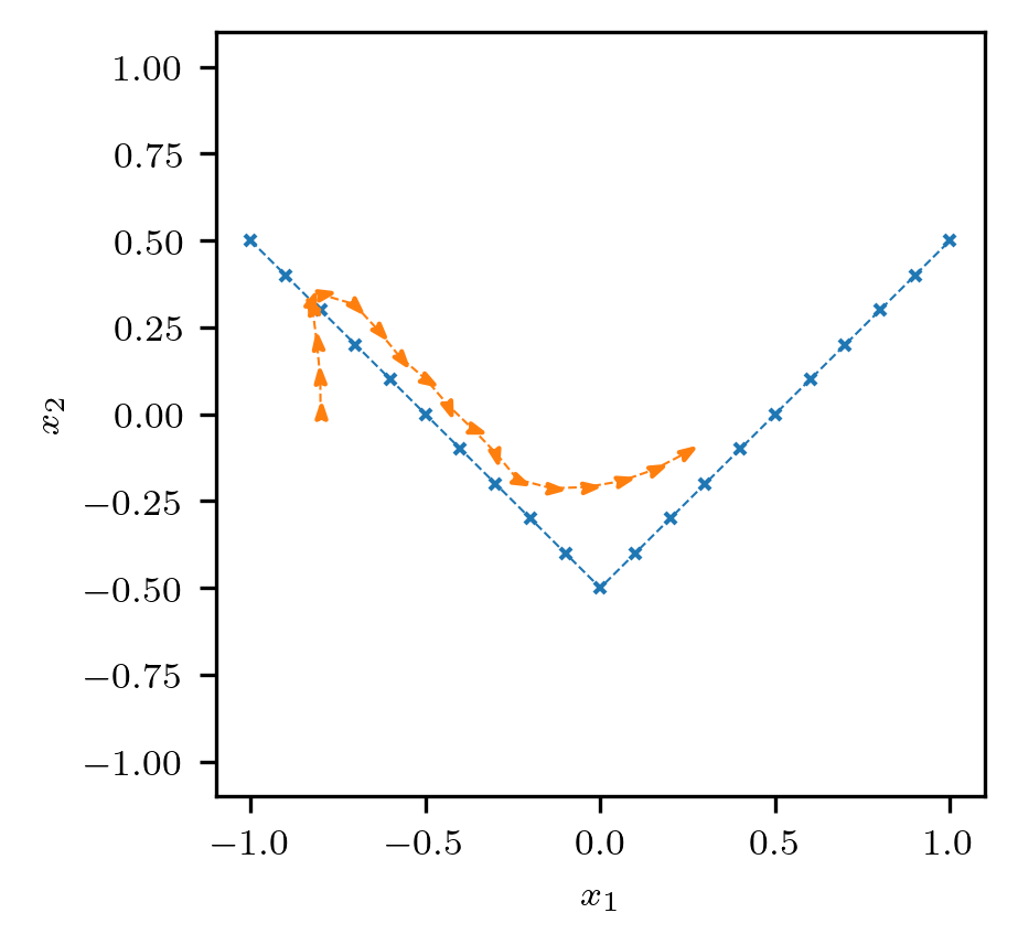
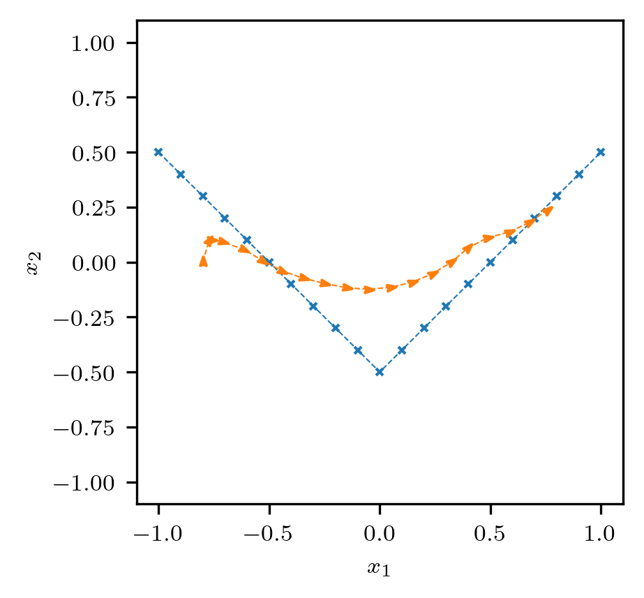
Figure 1. Nonholonomic vehicle trajectory using stochastic optimal control (top) and using dynamic programming (bottom) over a time horizon of $N=20$. The dashed blue line shows the target trajectory, and the orange line shows the nonholonomic vehicle trajectory. Note that the dynamic programming trajectory better satisfies the terminal constraint.

We consider a target tracking problem using nonholonomic vehicle dynamics, given by:

(23) $$\dot{x}_{1} =u_{1}\cos(x_{3}), \dot{x}_{2} =u_{1}\sin(x_{3}), \dot{x}_{3} =u_{2},$$

where $\mathcal{X}\subseteq\mathbb{R}^{3}$, $\mathcal{U}\subseteq\mathbb{R}^{2}$, and we constrain the input such that $u_{1}\in[0.1,1]$, $u_{2}\in[-10,10]$. We then discretize the dynamics in time with sampling time $T_{s}$ and apply an affine stochastic disturbance $w\sim\mathcal{N}(0,\Sigma)$, $\Sigma=0.01I$. The goal is to minimize the distance to an object moving along the v-shaped trajectory shown in blue in Figure 1. We then collect a sample $\mathcal{S}=\{(x_{i},u_{i},y_{i})\}_{i=1}^{M}$, of size $M=2500$, and compute the optimal control actions using both the optimal control and dynamic programming algorithms in SOCKS with $\sigma=2$. The results are shown in Figure 1, and computation time took approximately $0.204$ seconds for the optimal control algorithm and $12.003$ seconds for the dynamic programming algorithm. We can see that the system more closely meets the terminal constraint using the dynamic programming algorithm, but the computation time increases dramatically, since we must compute a sequence of value functions.

4.8. Satellite Rendezvous and Docking

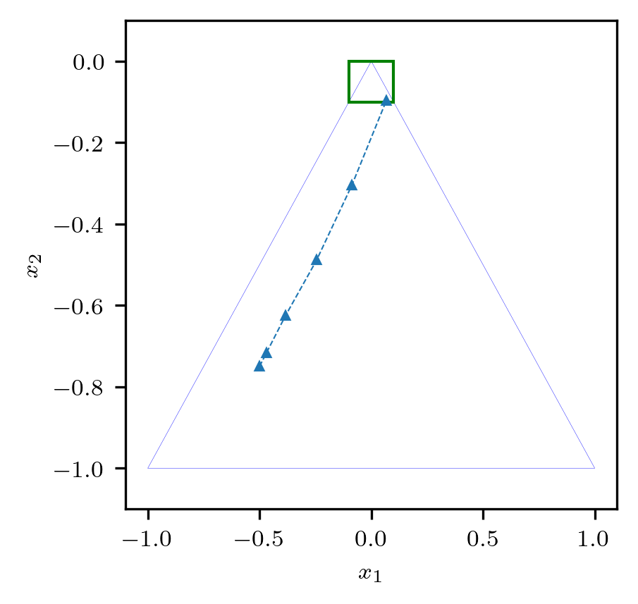
Figure 2. Optimal control for spacecraft rendezvous and docking problem with CWH dynamics. The goal is to reach a small region close to the origin (green square) while remaining within a line of sight cone (blue triangle). The trajectory of the system using the approximate stochastic optimal control algorithm is shown in blue.

We consider an example of spacecraft rendezvous and docking, in which one spacecraft must dock with another while remaining within a line of sight cone. The Clohessy-Wiltshire-Hill dynamics are given by,

(24) $$\ddot{x}-3\omega^{2}x-2\omega\dot{y} =F_{x}/m_{d}, \ddot{y}+2\omega\dot{x} =F_{y}/m_{d},$$

with state $z=[x,y,\dot{x},\dot{y}]^{\top}\in\mathcal{X}\subseteq\mathbb{R}^{4}$, input $u=[F_{x},F_{y}]^{\top}\in\mathcal{U}\subseteq\mathbb{R}^{2}$, where $\mathcal{U}=[-0.1,0.1]\times[-0.1,0.1]$, and parameters $\omega$, $m_{d}$. From (Lesser et al., 2013), the dynamics in (24) can be written as a discrete-time LTI system $z_{t+1}=Az_{t}+Bu_{t}+w_{t}$ with an additive Gaussian disturbance $w_{k}\sim\mathcal{N}(0,\Sigma)$, where $\Sigma=\textnormal{diag}([1\times 10^{-4},1\times 10^{-4},5\times 10^{-8},5\times 10^{-8}])$. We apply the stochastic optimal control algorithm in SOCKS to the CWH system using the kernel bandwidth parameter $\sigma=0.1$ and with a sample $\mathcal{S}=\{(x_{i},u_{i},y_{i})\}_{i=1}^{M}$ of size $M=2{,}500$ with points $x_{i}$ sampled uniformly in the region $[-1.1,1.1]\times[-1.1,1.1]\times[-0.06,0.06]\times[-0.06,0.06]$, $u_{i}\in[-0.05,0.05]^{2}$, and $y_{i}\sim Q(\cdot\mid x_{i},u_{i})$. The result is shown in Figure 2, and computation time was approximately $0.203$ seconds.

4.9. Double Integrator System

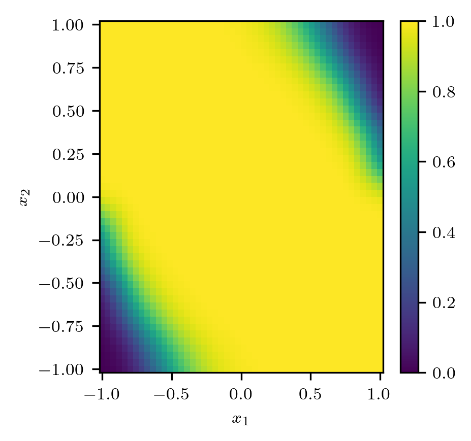
Figure 3. Stochastic reachability analysis of a double integrator system showing the maximal stochastic reachability safety probabilities with a safe set $\mathcal{K}=[-1,1]^{2}$, target set $\mathcal{T}=[-0.5,0.5]^{2}$, and time horizon $N=16$ for the terminal-hitting time problem.

We consider a stochastic double integrator system in order to showcase the stochastic reachability analysis. The dynamics of the system with sampling time $T_{s}$ are given by,

(25) $$x_{t+1}=\begin{bmatrix}1&T_{s}\\ 0&1\end{bmatrix}x_{t}+\begin{bmatrix}T_{s}^{2}/2\\ T_{s}\end{bmatrix}u_{t}+w_{t},$$

where $\mathcal{X}\subseteq\mathbb{R}^{2}$, $\mathcal{U}\subset\mathbb{R}$, and $w_{t}\sim\mathcal{N}(0,\Sigma)$, $\Sigma=0.01I$, is a random variable with a Gaussian distribution. We collect a sample $\mathcal{S}=\{(x_{i},u_{i},y_{i})\}_{i=1}^{M}$, $M=2{,}500$, taken i.i.d. from $Q$, a representation of the dynamics in (25) as a stochastic kernel, such that $x_{i}$ and $u_{i}$ are sampled uniformly from $\mathcal{X}$ and $\mathcal{U}$, respectively, with $x_{i}$ in the range $[-1.1,1.1]^{2}$ and $u_{i}$ in the range $[-1,1]$, and draw $y_{i}$ from $Q(\cdot\mid x_{i},u_{i})$. The safe set is defined as $\mathcal{K}=[-1,1]^{2}$ and the target set is defined as $\mathcal{T}=[-0.5,0.5]^{2}$. We then computed the stochastic reachability safety probabilities for both the terminal-hitting time problem and the first-hitting time problem at $T=10{,}000$ evaluation points using SOCKS and validated the result using Monte-Carlo. The computation time was $\approx 3$ seconds for both problems. The result is shown in Figure 3.

4.10. Forward Reachability

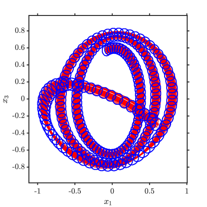
Figure 4. Approximate forward reachable set computed using the algorithm in (Thorpe et al., 2021a) with sample size $M=50$ and the Abel kernel with $\sigma=0.1$. The solid blue lines indicate the estimated support boundary of the distribution at each time step and the red lines indicate the sampled trajectories.

We then demonstrate the forward reachable set algorithm in SOCKS for a translational oscillations by a rotational actuator (TORA) system (Thorpe et al., 2021a). The dynamics of the system are given by,

(26) $$\dot{x}_{1} =x_{2}, \dot{x}_{2} =-x_{1}+0.1\sin(x_{3}), \dot{x}_{3} =x_{4}, \dot{x}_{4} =u,$$

where $\mathcal{X}\subseteq\mathbb{R}^{4}$, $\mathcal{U}\subset{R}$ and $u$ is a control input chosen by a neural network controller (Dutta et al., 2019). We then discretize the dynamics in time and apply an affine stochastic disturbance $w\sim\mathcal{N}(0,\Sigma)$, $\Sigma=0.01I$. We presume an initial distribution that is uniform over the region $[0.6,0.7]\times[-0.7,-0.6]\times[-0.4,-0.3]\times[0.5,0.6]$ and collect a sample $\mathcal{S}$ consisting of $M=50$ simulated trajectories over a time horizon $N=200$. Then, we apply the forward reachable set estimation algorithm and compute a classifier using (22) that estimates the support of the distribution at each time step. The results are shown in Figure 4, and the computation time was approximately $50.6$ seconds.

4.11. Scalability & Computation Time

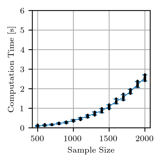
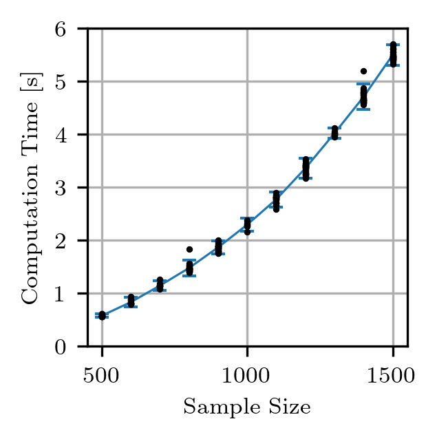
Figure 5. Computation time of the stochastic optimal control algorithm (left), the dynamic programming algorithm (center), and the maximal stochastic reachability algorithm (right) as a function of sample size $M$. The black dots indicate the computation time at each trial, and the blue bars indicate the 95% confidence interval over 16 trials. The computation time scales polynomially as a function of sample size, and is generally $\mathcal{O}(M^{3})$.

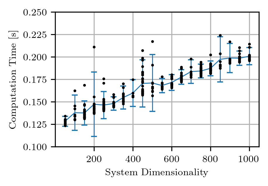
Figure 6. Computation time of the stochastic optimal control algorithm for an $n$-dimensional integrator system as a function of system dimensionality. The blue bars indicate the 95% confidence interval over 16 trials. The computation time scales roughly linearly with the dimensionality of the system.

We now present a brief discussion of the scalability and computational complexity of the algorithms. As shown in (Thorpe and Oishi, 2020; Thorpe et al., 2021b; Thorpe and Oishi, 2021), the sample size $M$ used to compute the empirical distribution embedding $\hat{m}(x,u)$ presents the most significant computational burden, and is generally $\mathcal{O}(M^{3})$ due to the presence of the matrix inversion in (16). We demonstrate this empirically for the algorithms presented in SOCKS in Figure 5. We calculated the computation times for the algorithms over 16 runs for different values of $M$, and computed the statistical average and the 95% confidence interval. The black dots indicate the empirically measured times, and the blue bars indicate the confidence interval for our algorithm. We can see that the computation times scale polynomially with the sample size $M$, as expected. This can be prohibitive, since the quality of the kernel-based approximation improves as the sample size tends to infinity. Nevertheless, several approximative speedup techniques (e.g. (Grünewälder et al., 2012; Rahimi and Recht, 2007)) have been developed to alleviate the computational burden, and have been shown to reduce the computational complexity to $\mathcal{O}(M\log M)$. These techniques are not currently implemented in SOCKS, but we plan to include them as part of a future release. As mentioned in (Thorpe and Oishi, 2020), the complexity of the kernel-based algorithms scales roughly linearly with the dimensionality of the system. This is primarily due to the fact that the system dimensionality only plays a role in the kernel evaluations, and does not significantly affect the computation of the empirical embedding $\hat{m}(x,u)$. We demonstrate this empirically for an $n$-dimensional stochastic chain of integrators system as in (25) (see (Thorpe and Oishi, 2020)), where we choose a fixed sample size $M=1000$ and vary the system dimensionality from $n=50$ to $n=1000$. The computation times are shown in Figure 6. We can see in Figure 6 that as the system is dimensionality is increased, the computation time increases roughly linearly. However, as mentioned in (Thorpe and Oishi, 2020), for high-dimensional systems, the sample size needed to fully characterize the dynamics and the uncertainty increases as the system dimensionality increases, which can be prohibitive for the reasons mentioned above.

5. Conclusion & Future Work

In this paper, we introduced SOCKS, a toolbox for approximate stochastic optimal control and approximate stochastic reachability based on a data-driven statistical learning technique known as kernel embeddings of distributions. We have demonstrated the capabilities of the toolbox on a simple stochastic chain of integrators example, a more realistic satellite rendezvous and docking example, a target tracking scenario using nonlinear nonholonomic vehicle dynamics, and on a forward reachable set estimation problem. The approaches used in SOCKS are scalable, computationally efficient, and model-free. We plan to introduce additional kernel-based algorithms and features to SOCKS, such as the capability to handle neural network reachability analysis, trajectory optimization, and chance-constrained optimization.

Appendix A Stochastic Optimal Control

In this section, we give an overview of the stochastic optimal control algorithm. Additional details are provided in (Thorpe and Oishi, 2021). Given a sample $\mathcal{S}$ as in (2), taken i.i.d. from $Q$, we can compute an empirical estimate $\hat{m}(x,u)$ of the conditional distribution embedding $m(x,u)$. By assumption 3, we assume that the objective and constraints can be decomposed as $f_{i}(x,u)=f_{i}^{x}(x)+f_{i}^{u}(u)$. Assuming the objective function $f_{0}$ and constraints $f_{i}$, $i=1,\ldots,p$, are elements of the RKHS $\mathscr{H}$, we can approximate the expectation with respect to $Q(\cdot\mid x,u)$ via the reproducing property of $k$ in $\mathscr{H}$,

$$\int_{\mathcal{U}}\int_{\mathcal{X}}f_{i}(y,v)Q(\mathrm{d}y\mid x,v)\pi_{t}(\mathrm{d}v\mid x)$$

(27) $$\qquad=\int_{\mathcal{U}}\int_{\mathcal{X}}f_{i}^{x}(y)Q(\mathrm{d}y\mid x,v)+f_{i}^{u}(v)\pi_{t}(\mathrm{d}v\mid x)$$

(28) $$\qquad\approx\int_{\mathcal{U}}\langle f_{i}^{x},\hat{m}(x,v)\rangle_{\mathscr{H}}+f_{i}^{u}(v)\pi_{t}(\mathrm{d}v\mid x)$$

(29) $$\qquad=\int_{\mathcal{U}}\boldsymbol{f}_{i}^{x}{}^{\top}W\Psi k(x,\cdot)l(v,\cdot)+f_{i}^{u}(v)\pi_{t}(\mathrm{d}v\mid x),$$

for all $f_{i}$, $i=0,1,\ldots,p$. Then, following (Thorpe and Oishi, 2021), we propose the following form for the approximation of the policy. Given a set $\mathcal{A}\subset\mathcal{U}$ of admissible control actions, $\mathcal{A}=\{\tilde{u}_{j}\}_{i=1}^{P}$, $P\in\mathbb{N}$, we have

(30) $$\hat{p}_{t}(x)=\sum_{j=1}^{P}\gamma(x)l(\tilde{u}_{j},\cdot).$$

We can write (29) using the policy approximation in (30), and obtain

$$\int_{\mathcal{U}}\boldsymbol{f}_{i}^{x}{}^{\top}W\Psi k(x,\cdot)l(v,\cdot)+f_{i}^{u}(v)\pi_{t}(\mathrm{d}v\mid x)$$

(31) $$\qquad\approx\boldsymbol{f}_{i}^{x}{}^{\top}W\Psi\Upsilon^{\top}k(x,\cdot)\gamma(x)+\boldsymbol{f}_{i}^{u}{}^{\top}\gamma(x),$$

where $\Upsilon$ is a feature vector with elements $\Upsilon_{j}=l(\tilde{u}_{j},\cdot)$. We use this representation in the optimal control problem in order to approximate the objective and constraints. The following problem is approximately equivalent to the optimal control problem in (3),

(32a) $$\min_{\gamma\in\mathbb{R}^{P}}\quad \boldsymbol{f}_{0}^{x}{}^{\top}W\Psi\Upsilon^{\top}k(x,\cdot)\gamma(x)+\boldsymbol{f}_{0}^{u}{}^{\top}\gamma(x)$$

(32b) s.t. $$\boldsymbol{f}_{i}^{x}{}^{\top}W\Psi\Upsilon^{\top}k(x,\cdot)\gamma(x)+\boldsymbol{f}_{i}^{u}{}^{\top}\gamma(x)\leq 0,i=1,\ldots,p$$

Furthermore, as the number of observations $M$ in the sample $\mathcal{S}$ and the number of admissible control actions $P$ in $\mathcal{A}$ tends to infinity, the solution to the approximate problem converges in probability to the true solution (Thorpe and Oishi, 2021). See Appendix B for a more detailed discussion of convergence. However, the optimization problem is unbounded below. In order to ensure feasibility, following (Thorpe and Oishi, 2021), we add an additional constraint such that $\gamma(x)$ lies in the probability simplex $\gamma(x)\in\{a\mid\boldsymbol{1}^{\top}a=1,0\preceq a\}$, where $\boldsymbol{1}$ is a vector of all ones. Thus, the approximate optimal control problem becomes

(33a) $$\min_{\gamma\in\mathbb{R}^{P}}\quad \boldsymbol{f}_{0}^{x}{}^{\top}W\Psi\Upsilon^{\top}k(x,\cdot)\gamma(x)+\boldsymbol{f}_{0}^{u}{}^{\top}\gamma(x)$$

(33b) s.t. $$\boldsymbol{f}_{i}^{x}{}^{\top}W\Psi\Upsilon^{\top}k(x,\cdot)\gamma(x)+\boldsymbol{f}_{i}^{u}{}^{\top}\gamma(x)\leq 0,i=1,\ldots,p$$

(33c) $$\boldsymbol{1}^{\top}\gamma(x)=1$$

(33d) $$0\preceq\gamma(x)$$

This is a linear program, and can be solved efficiently, e.g. via several commonly-used interior point or simplex algorithms (Boyd et al., 2004). Additionally, this representation can be used to solve a backward-in-time stochastic optimal control problem (dynamic programming). See (Thorpe and Oishi, 2021) for more details.

Appendix B Stability & Convergence

We now seek to characterize the quality of the approximation and the conditions for its convergence. The convergence properties of kernel distribution embeddings are well-studied in literature. See e.g. (Song et al., 2009, 2010b; Grünewälder et al., 2012; Park and Muandet, 2020) for more information. However, the nuances of the different convergence results for kernel distribution embeddings means that the results do not always generalize well to all problems under different kernel choices. For instance, the result in (Song et al., 2009, Theorem 6) shows that the empirical estimate $\hat{m}(x,u)$ converges in probability to the true embedding $m(x,u)$ at a rate of $\mathcal{O}_{p}((M\lambda)^{-1/2}+\lambda^{1/2})$, where $\lambda$ is the regularization parameter in (14) and $M$ is the sample size, but (Song et al., 2009) assumes that the RKHS is finite-dimensional, which does not hold for common kernel choices such as the Gaussian RBF kernel. Thus, we present convergence results for the approximate stochastic optimal control problem based in the theory of algorithmic stability (Bousquet and Elisseeff, 2002). Our result is close to the result presented in (Park and Muandet, 2020). We first seek to characterize the convergence of the estimate $\hat{m}(x,u)$ in (16) to its actual counterpart $m(x,u)$ in (10). For simplicity of notation, we define the operator $k_{x}:\mathcal{X}\to\mathbb{R}$ for all $x\in\mathcal{X}$ via $k_{x}(x^{\prime})=k(x,x^{\prime})$. Recall that the estimate $\hat{m}$ is in a vector-valued RKHS $\mathscr{Q}$ and is the solution to the regularized least-squares problem in (14). Let $J:\mathscr{H}\times\mathscr{H}\to\mathbb{R}$ be a real-valued cost function, defined by

(34) $$J(k_{y},\hat{m}(x,u))\coloneqq\lVert k_{y}-\hat{m}(x,u)\rVert_{\mathscr{H}}^{2}.$$

Let $\mathcal{Z}=\mathcal{X}\times\mathcal{U}\times\mathcal{X}$. We define the loss function $\upsilon:\mathscr{Q}\times\mathcal{Z}\to\mathbb{R}$, given by

(35) $$\upsilon(\hat{m},(x,u,y))=J(k_{y},\hat{m}(x,u)).$$

The risk, denoted by $R(\hat{m})$, measures the expected loss (error) of the solution $\hat{m}$ to the regularized least-squares learning problem, and is defined as

(36) $$R(\hat{m})\coloneqq\int_{\mathcal{X}}\upsilon(\hat{m},(x,u,y))Q(\mathrm{d}y\mid x,u).$$

However, we cannot compute the risk directly since $Q$ is unknown by Assumption 1. Thus, we seek to bound the risk by its empirical counterpart. Given a sample $\mathcal{S}\in\mathcal{Z}^{M}$ as in (2), the empirical risk, denoted by $R_{\mathcal{S}}(\hat{m})$, also known as the empirical error, measures the actual loss of the learning problem, and is defined as

(37) $$R_{\mathcal{S}}(\hat{m}) \coloneqq\frac{1}{M}\sum_{i=1}^{M}\upsilon(\hat{m},(x_{i},u_{i},y_{i}))+\lambda\lVert\hat{m}\rVert_{\mathscr{Q}}^{2}$$

(38) $$=\frac{1}{M}\sum_{i=1}^{M}\lVert k_{y_{i}}-\hat{m}(x_{i},u_{i})\rVert_{\mathscr{H}}^{2}+\lambda\lVert\hat{m}\rVert_{\mathscr{Q}}^{2}.$$

We use $\hat{m}$ to denote the solution to the regularized least squares problem in (14), and let $\hat{m}^{\backslash i}$ denote the solution when a single observation is removed from $\mathcal{S}$ and let $\hat{m}^{i}$ denote the solution when the $i^{\rm th}$ observation is changed. We use $\hat{m}^{\backslash i}$ and $\hat{m}^{i}$ in the following to assess the stability of the learning algorithm under minor changes to the sample $\mathcal{S}$ used to construct the estimate $\hat{m}$. We present the following definition, modified from (Bousquet and Elisseeff, 2002), which allows us to characterize the stability of the learning algorithm with respect to the regularized least-squares problem in (14).

Definition 7 ($\sigma$-admissible, (Bousquet and Elisseeff, 2002, Definition 19)).

A loss function $\upsilon$ on $\mathscr{Q}\times\mathcal{Z}$ is $\sigma$-admissible with respect to $\mathscr{Q}$ if the associated cost function is convex with respect to its first argument and the following condition holds,

(39) $$\lvert J(k_{y_{1}},k_{y^{\prime}})-J(k_{y_{2}},k_{y^{\prime}})\rvert\leq\sigma\lVert k_{y_{1}}-k_{y_{2}}\rVert_{\mathscr{H}}$$

for all $k_{y^{\prime}}\in\mathscr{H}$ and $k_{y_{1}},k_{y_{2}}\in\mathcal{D}$, where

(40) $$\mathcal{D}=\{k_{y}\mid\exists f\in\mathscr{Q},\exists(x,u)\in\mathcal{X}\times\mathcal{U},f(x,u)=k_{y}\}$$

is the domain of the first argument of $J$.

We now seek to verify that the loss function $\upsilon$ pertaining to the regularized least-squares problem is $\sigma$-admissible with respect to $\mathscr{Q}$. To this aim, we present the following proposition.

Proposition 1.

The loss function given by

(41) $$\upsilon(\hat{m},(x,u,y))=J(\hat{m}(x,u),k_{y})=\lVert k_{y}-\hat{m}(x,u)\rVert_{\mathscr{H}}^{2}$$

is $\sigma$-admissible with respect to $\mathscr{Q}$.

The proof follows (Bousquet and Elisseeff, 2002, Lemma 20), which shows that the loss function using a Hilbert space norm is $\sigma$-admissible, where $\sigma$ depends on the choice of kernel and the corresponding Hilbert space of functions $\mathscr{H}$. We now present the following definition from (Bousquet and Elisseeff, 2002), modified to our particular formulation, which bounds the maximum difference in the loss function under minor variations to the sample $\mathcal{S}$.

Definition 8 (uniform stability, (Bousquet and Elisseeff, 2002, Definition 6)).

A learning algorithm has uniform stability $\alpha$ with respect to the loss function $\upsilon$ if the following holds:

(42) $$\lVert\upsilon(\hat{m},\cdot)-\upsilon(\hat{m}^{\backslash i},\cdot)\rVert_{\infty}\leq\alpha,$$

for all $\mathcal{S}\in\mathcal{Z}^{M}$ and $i=1,\ldots,M$.

In addition, an algorithm with uniform stability has the following property:

(43) $$\lvert\upsilon(\hat{m},\cdot)-\upsilon(\hat{m}^{i},\cdot)\rvert\leq 2\alpha.$$

As a consequence of the above definitions, (Bousquet and Elisseeff, 2002) shows that the regularized least-squares problem in the scalar RKHS case has uniform stability. We modify (Bousquet and Elisseeff, 2002, Theorem 22) to a vector-valued RKHS in the following theorem.

Theorem 1.

Let $\mathscr{H}$ be an RKHS with kernel $k$ and $\mathscr{Q}$ be a vector-valued RKHS of functions on $\mathcal{X}\times\mathcal{U}$ mapping to $\mathscr{H}$. Let $k$ be bounded by $\rho<\infty$, and let $\upsilon$ be a $\sigma$-admissible loss function with respect to $\mathscr{Q}$. Then the learning algorithm given by

(44) $$\hat{m}=\arg\min_{f\in\mathscr{Q}}\frac{1}{M}\sum_{i=1}^{M}\upsilon(f,(y_{i},x_{i},u_{i}))+\lambda\lVert f\rVert_{\mathscr{Q}}^{2},$$

has uniform stability $\alpha$ with respect to $\upsilon$ with

(45) $$\alpha\leq\frac{\sigma^{2}\rho^{2}}{2\lambda M}.$$

We can ensure boundedness of the kernel of $\mathscr{Q}$ using the principle of uniform boundedness (also known as the Banach-Steinhaus theorem), since the kernel $k$ is bounded by $\rho$. Then the proof follows directly from (Bousquet and Elisseeff, 2002, Theorem 22). We use this result to show that the regularized least-squares problem in (14) has uniform stability with respect to $\upsilon$.

Theorem 2 ((Bousquet and Elisseeff, 2002, Theorem 12)).

Let $A$ be an algorithm with uniform stability $\alpha$ with respect to a loss function $\upsilon$ such that $0\leq\upsilon(\hat{m},(x,u,y))\leq B$, for all $(x,u,y)\in\mathcal{Z}$ and all sets $\mathcal{S}$. Then for any $M\geq 1$ and any $\delta\in(0,1)$ the following bounds hold with probability $1-\delta$ of the random draw of the sample $\mathcal{S}$:

(46) $$R(\hat{m})\leq R_{\mathcal{S}}(\hat{m})+2\alpha+(4M\alpha+B)\sqrt{\frac{\log(1/\delta)}{2M}}.$$

Thus, using Theorem 2 with $\alpha$ given by (45) from Theorem 1, we have that for any $M\geq 1$ and any $\delta\in(0,1)$, with probability $1-\delta$, the risk $R$ is bounded by:

(47) $$R(\hat{m})\leq R_{\mathcal{S}}(\hat{m})+\frac{\sigma^{2}\rho^{2}}{\lambda M}+\biggl{(}\frac{2\sigma^{2}\rho^{2}}{\lambda}+\rho\biggr{)}\sqrt{\frac{\log(1/\delta)}{2M}},$$

which shows that as the sample size $M$ increases, the empirical embedding $\hat{m}(x,u)$ in (16) converges in probability to the true embedding $m(x,u)$ in (10). Thus, the approximation of the expectations in (33) converge in probability to the true expectations, and the approximate optimization problems computed using the estimate $\hat{m}(x,u)$ converge to the true optimization problems as $M$ increases. Similarly, the approximate policy $\hat{p}(x)$ in (30) has the form of an empirical conditional distribution embedding as in (16), which suggests that the approximate policy (and consequently the approximately optimal control action) obtained via (33) also converges in probability as the number of admissible control actions $P$ in (30) is increased.

References

- (1)
- Abadi et al. (2015) Martín Abadi, Ashish Agarwal, Paul Barham, Eugene Brevdo, Zhifeng Chen, Craig Citro, Greg S. Corrado, Andy Davis, Jeffrey Dean, Matthieu Devin, Sanjay Ghemawat, Ian Goodfellow, Andrew Harp, Geoffrey Irving, Michael Isard, Yangqing Jia, Rafal Jozefowicz, Lukasz Kaiser, Manjunath Kudlur, Josh Levenberg, Dandelion Mané, Rajat Monga, Sherry Moore, Derek Murray, Chris Olah, Mike Schuster, Jonathon Shlens, Benoit Steiner, Ilya Sutskever, Kunal Talwar, Paul Tucker, Vincent Vanhoucke, Vijay Vasudevan, Fernanda Viégas, Oriol Vinyals, Pete Warden, Martin Wattenberg, Martin Wicke, Yuan Yu, and Xiaoqiang Zheng. 2015. TensorFlow: Large-Scale Machine Learning on Heterogeneous Systems. https://www.tensorflow.org/ Software available from tensorflow.org.
- Abate et al. (2019) Alessandro Abate, Henk Blom, Nathalie Cauchi, Kurt Degiorgio, Martin Fränzle, Ernst Moritz Hahn, Sofie Haesaert, Hao Ma, Meeko Oishi, Carina Pilch, et al. 2019. ARCH-COMP19 category report: Stochastic modelling. EPiC Series in Computing 61 (2019), 62–102.
- Abate et al. (2020) Alessandro Abate, Henk Blom, Nathalie Cauchi, Joanna Delicaris, Arnd Hartmanns, Mahmoud Khaled, Abolfazl Lavaei, Carina Pilch, Anne Remke, Stefan Schupp, et al. 2020. ARCH-COMP20 Category Report: Stochastic Models. EPiC Series in Computing 74 (2020), 76–106.
- Abate et al. (2018) Alessandro Abate, HAP Blom, Nathalie Cauchi, Sofie Haesaert, Arnd Hartmanns, Kendra Lesser, Meeko Oishi, Vignesh Sivaramakrishnan, and Sadegh Soudjani. 2018. ARCH-COMP18 Category Report: Stochastic Modelling. EPiC Series in Computing 54 (2018).
- Abate et al. (2008) Alessandro Abate, Maria Prandini, John Lygeros, and Shankar Sastry. 2008. Probabilistic reachability and safety for controlled discrete time stochastic hybrid systems. Automatica 44, 11 (2008), 2724–2734.
- Aronszajn (1950) Nachman Aronszajn. 1950. Theory of reproducing kernels. Transactions of the American mathematical society 68, 3 (1950), 337–404.
- Bertsekas and Shreve (1978) Dimitri P Bertsekas and Steven E Shreve. 1978. Stochastic optimal control: the discrete time case. Elsevier.
- Bousquet and Elisseeff (2002) Olivier Bousquet and André Elisseeff. 2002. Stability and generalization. The Journal of Machine Learning Research 2 (2002), 499–526.
- Boyd et al. (2004) Stephen Boyd, Stephen P Boyd, and Lieven Vandenberghe. 2004. Convex optimization. Cambridge university press.
- Brockman et al. (2016) Greg Brockman, Vicki Cheung, Ludwig Pettersson, Jonas Schneider, John Schulman, Jie Tang, and Wojciech Zaremba. 2016. Openai gym. arXiv preprint arXiv:1606.01540 (2016).
- Cauchi and Abate (2019) Nathalie Cauchi and Alessandro Abate. 2019. StocHy - Automated Verification and Synthesis of Stochastic Processes: Poster Abstract. In Proceedings of the 22nd ACM International Conference on Hybrid Systems: Computation and Control (HSCC ’19). Association for Computing Machinery, New York, NY, USA, 258–259.
- Chollet et al. (2015) François Chollet et al. 2015. Keras. https://keras.io.
- Çınlar (2011) Erhan Çınlar. 2011. Probability and Stochastics. Vol. 261. Springer Science & Business Media.
- De Vito et al. (2014) Ernesto De Vito, Lorenzo Rosasco, and Alessandro Toigo. 2014. Learning sets with separating kernels. Applied and Computational Harmonic Analysis 37, 2 (2014), 185–217.
- Dehnert et al. (2017) Christian Dehnert, Sebastian Junges, Joost-Pieter Katoen, and Matthias Volk. 2017. A Storm is Coming: A Modern Probabilistic Model Checker. In Computer Aided Verification, Rupak Majumdar and Viktor Kunčak (Eds.). Springer International Publishing, Cham, 592–600.
- Deisenroth et al. (2009) Marc Peter Deisenroth, Carl Edward Rasmussen, and Jan Peters. 2009. Gaussian process dynamic programming. Neurocomputing 72, 7-9 (2009), 1508–1524.
- Djeumou and Topcu (2021) Franck Djeumou and Ufuk Topcu. 2021. Learning to Reach, Swim, Walk and Fly in One Trial: Data-Driven Control with Scarce Data and Side Information. arXiv preprint arXiv:2106.10533 (2021).
- Djeumou et al. (2021) Franck Djeumou, Aditya Zutshi, and Ufuk Topcu. 2021. On-the-fly, data-driven reachability analysis and control of unknown systems: an F-16 aircraft case study. In Proceedings of the 24th International Conference on Hybrid Systems: Computation and Control. 1–2.
- Dutta et al. (2019) Souradeep Dutta, Xin Chen, Susmit Jha, Sriram Sankaranarayanan, and Ashish Tiwari. 2019. Sherlock-A tool for verification of neural network feedback systems. In International Conference on Hybrid Systems: Computation and Control. 262–263.
- Garcıa and Fernández (2015) Javier Garcıa and Fernando Fernández. 2015. A comprehensive survey on safe reinforcement learning. Journal of Machine Learning Research 16, 1 (2015), 1437–1480.
- Geretti et al. (2020) Luca Geretti, Julien Alexandre Dit Sandretto, Matthias Althoff, Luis Benet, Alexandre Chapoutot, Xin Chen, Pieter Collins, Marcelo Forets, Daniel Freire, Fabian Immler, et al. 2020. Arch-comp20 category report: Continuous and hybrid systems with nonlinear dynamics. EPiC Series in Computing 74 (2020), 49–75.
- Grünewälder et al. (2012) Steffen Grünewälder, Guy Lever, Luca Baldassarre, Sam Patterson, Arthur Gretton, and Massimilano Pontil. 2012. Conditional mean embeddings as regressors. In Proceedings of the 29th International Coference on International Conference on Machine Learning. 1803–1810.
- Grünewälder et al. (2012) Steffen Grünewälder, Guy Lever, Luca Baldassarre, Massimilano Pontil, and Arthur Gretton. 2012. Modelling Transition Dynamics in MDPs with RKHS Embeddings. In Proceedings of the 29th International Coference on International Conference on Machine Learning (ICML’12). Omnipress, Madison, WI, USA, 1603–1610.
- Katz et al. (2019) Guy Katz, Derek Huang, Duligur Ibeling, Kyle Julian, Christopher Lazarus, Rachel Lim, Parth Shah, Shantanu Thakoor, Haoze Wu, Aleksandar Zeljić, David L. Dill, Mykel Kochenderfer, and Clark Barrett. 2019. The Marabou Framework for Verification and Analysis of Deep Neural Networks. In Computer Aided Verification, Isil Dillig and Serdar Tasiran (Eds.). Springer International Publishing, Cham, 443–452.
- Kingston et al. (2018) Zachary Kingston, Mark Moll, and Lydia E Kavraki. 2018. Sampling-based methods for motion planning with constraints. Annual review of control, robotics, and autonomous systems 1 (2018), 159–185.
- Kwiatkowska et al. (2011) Marta Kwiatkowska, Gethin Norman, and David Parker. 2011. PRISM 4.0: Verification of probabilistic real-time systems. In International conference on computer aided verification. Springer, 585–591.
- Lavaei et al. (2020) Abolfazl Lavaei, Mahmoud Khaled, Sadegh Soudjani, and Majid Zamani. 2020. AMYTISS: A Parallelized Tool on Automated Controller Synthesis for Large-Scale Stochastic Systems. In Proceedings of the 23rd International Conference on Hybrid Systems: Computation and Control (HSCC ’20). Association for Computing Machinery, New York, NY, USA, Article 31, 2 pages.
- Lesser et al. (2013) Kendra Lesser, Meeko Oishi, and R Scott Erwin. 2013. Stochastic reachability for control of spacecraft relative motion. In 52nd IEEE Conference on Decision and Control. IEEE, 4705–4712.
- Lever and Stafford (2015) Guy Lever and Ronnie Stafford. 2015. Modelling Policies in MDPs in Reproducing Kernel Hilbert Space. In Proceedings of the Eighteenth International Conference on Artificial Intelligence and Statistics (Proceedings of Machine Learning Research), Guy Lebanon and S. V. N. Vishwanathan (Eds.), Vol. 38. PMLR, San Diego, California, USA, 590–598.
- Marinho et al. (2016) Zita Marinho, Byron Boots, Anca Dragan, Arunkumar Byravan, Geoffrey J. Gordon, and Siddhartha Srinivasa. 2016. Functional Gradient Motion Planning in Reproducing Kernel Hilbert Spaces. In Proceedings of Robotics: Science and Systems. AnnArbor, Michigan. https://doi.org/10.15607/RSS.2016.XII.046
- Micchelli and Pontil (2005) Charles A Micchelli and Massimiliano Pontil. 2005. On learning vector-valued functions. Neural computation 17, 1 (2005), 177–204.
- Park and Muandet (2020) Junhyung Park and Krikamol Muandet. 2020. A measure-theoretic approach to kernel conditional mean embeddings. Advances in Neural Information Processing Systems 33 (2020).
- Paszke et al. (2019) Adam Paszke, Sam Gross, Francisco Massa, Adam Lerer, James Bradbury, Gregory Chanan, Trevor Killeen, Zeming Lin, Natalia Gimelshein, Luca Antiga, Alban Desmaison, Andreas Kopf, Edward Yang, Zachary DeVito, Martin Raison, Alykhan Tejani, Sasank Chilamkurthy, Benoit Steiner, Lu Fang, Junjie Bai, and Soumith Chintala. 2019. PyTorch: An Imperative Style, High-Performance Deep Learning Library. In Advances in Neural Information Processing Systems 32, H. Wallach, H. Larochelle, A. Beygelzimer, F. d'Alché-Buc, E. Fox, and R. Garnett (Eds.). Curran Associates, Inc., 8024–8035.
- Pedregosa et al. (2011) F. Pedregosa, G. Varoquaux, A. Gramfort, V. Michel, B. Thirion, O. Grisel, M. Blondel, P. Prettenhofer, R. Weiss, V. Dubourg, J. Vanderplas, A. Passos, D. Cournapeau, M. Brucher, M. Perrot, and E. Duchesnay. 2011. Scikit-learn: Machine Learning in Python. Journal of Machine Learning Research 12 (2011), 2825–2830.
- Rahimi and Recht (2007) Ali Rahimi and Benjamin Recht. 2007. Random Features for Large-Scale Kernel Machines. In Advances in Neural Information Processing Systems, J. Platt, D. Koller, Y. Singer, and S. Roweis (Eds.), Vol. 20. Curran Associates, Inc. https://proceedings.neurips.cc/paper/2007/file/013a006f03dbc5392effeb8f18fda755-Paper.pdf
- Rasmussen and Williams (2006) Carl Edward Rasmussen and Chris Williams. 2006. Gaussian Processes for Machine Learning. MIT Press.
- Ray et al. (2019) Alex Ray, Joshua Achiam, and Dario Amodei. 2019. Benchmarking safe exploration in deep reinforcement learning. (2019).
- Reddy et al. (2020) Siddharth Reddy, Anca Dragan, Sergey Levine, Shane Legg, and Jan Leike. 2020. Learning human objectives by evaluating hypothetical behavior. In International Conference on Machine Learning. PMLR, 8020–8029.
- Rosolia and Borrelli (2017) Ugo Rosolia and Francesco Borrelli. 2017. Learning model predictive control for iterative tasks. a data-driven control framework. IEEE Trans. Automat. Control 63, 7 (2017), 1883–1896.
- Rosolia and Borrelli (2019) Ugo Rosolia and Francesco Borrelli. 2019. Sample-based learning model predictive control for linear uncertain systems. In 2019 IEEE 58th Conference on Decision and Control (CDC). IEEE, 2702–2707.
- Schölkopf et al. (2002) Bernhard Schölkopf, Alexander J Smola, Francis Bach, et al. 2002. Learning with kernels: support vector machines, regularization, optimization, and beyond. MIT press.
- Shmarov and Zuliani (2015) Fedor Shmarov and Paolo Zuliani. 2015. ProbReach: Verified Probabilistic Delta-Reachability for Stochastic Hybrid Systems. In Proceedings of the 18th International Conference on Hybrid Systems: Computation and Control (HSCC ’15). Association for Computing Machinery, New York, NY, USA, 134–139. https://doi.org/10.1145/2728606.2728625
- Smola et al. (2007) Alex Smola, Arthur Gretton, Le Song, and Bernhard Schölkopf. 2007. A Hilbert space embedding for distributions. In International Conference on Algorithmic Learning Theory. Springer, 13–31.
- Song et al. (2010a) Le Song, Byron Boots, Sajid M. Siddiqi, Geoffrey Gordon, and Alex Smola. 2010a. Hilbert Space Embeddings of Hidden Markov Models. In Proceedings of the 27th International Conference on International Conference on Machine Learning (ICML’10). Omnipress, Madison, WI, USA, 991–998.
- Song et al. (2010b) Le Song, Arthur Gretton, and Carlos Guestrin. 2010b. Nonparametric Tree Graphical Models. In Proceedings of the Thirteenth International Conference on Artificial Intelligence and Statistics (Proceedings of Machine Learning Research), Yee Whye Teh and Mike Titterington (Eds.), Vol. 9. PMLR, Chia Laguna Resort, Sardinia, Italy, 765–772.
- Song et al. (2009) Le Song, Jonathan Huang, Alex Smola, and Kenji Fukumizu. 2009. Hilbert space embeddings of conditional distributions with applications to dynamical systems. In Proceedings of the 26th Annual International Conference on Machine Learning. 961–968.
- Soudjani et al. (2015) Sadegh Esmaeil Zadeh Soudjani, Caspar Gevaerts, and Alessandro Abate. 2015. FAUST 2 : Formal Abstractions of Uncountable-STate STochastic Processes. In International Conference on Tools and Algorithms for the Construction and Analysis of Systems, Vol. 9035. Springer International Publishing, 272–286.
- Steinwart and Christmann (2008) Ingo Steinwart and Andreas Christmann. 2008. Support Vector Machines. Springer Publishing Company, Incorporated.
- Summers and Lygeros (2010) Sean Summers and John Lygeros. 2010. Verification of discrete time stochastic hybrid systems: A stochastic reach-avoid decision problem. Automatica 46, 12 (2010), 1951–1961.
- Thorpe and Oishi (2020) Adam J. Thorpe and Meeko M. K. Oishi. 2020. Model-Free Stochastic Reachability Using Kernel Distribution Embeddings. IEEE Control Systems Letters 4, 2 (2020), 512–517.
- Thorpe and Oishi (2021) Adam J. Thorpe and Meeko M. K. Oishi. 2021. Stochastic Optimal Control via Hilbert Space Embeddings of Distributions. In 2021 60th IEEE Conference on Decision and Control (CDC). 904–911. https://doi.org/10.1109/CDC45484.2021.9682801
- Thorpe et al. (2021a) Adam J. Thorpe, Kendric R. Ortiz, and Meeko M. K. Oishi. 2021a. Learning Approximate Forward Reachable Sets Using Separating Kernels. In Proceedings of the 3rd Conference on Learning for Dynamics and Control (Proceedings of Machine Learning Research), Ali Jadbabaie, John Lygeros, George J. Pappas, Pablo A. Parrilo, Benjamin Recht, Claire J. Tomlin, and Melanie N. Zeilinger (Eds.), Vol. 144. PMLR, 201–212.
- Thorpe et al. (2021b) Adam J. Thorpe, Kendric R. Ortiz, and Meeko M. K. Oishi. 2021b. SReachTools Kernel Module: Data-Driven Stochastic Reachability Using Hilbert Space Embeddings of Distributions. In 2021 60th IEEE Conference on Decision and Control (CDC). 5073–5079. https://doi.org/10.1109/CDC45484.2021.9683169
- Thorpe et al. (2021c) Adam J. Thorpe, Vignesh Sivaramakrishnan, and Meeko M. K. Oishi. 2021c. Approximate Stochastic Reachability for High Dimensional Systems. In 2021 American Control Conference (ACC). 1287–1293.
- Tran et al. (2020) Hoang-Dung Tran, Patrick Musau, Diego Manzanas Lopez, Xiaodong Yang, Luan Viet Nguyen, Weiming Xiang, and Taylor Johnson. 2020. NNV: A Tool for Verification of Deep Neural Networks and Learning-Enabled Autonomous Cyber-Physical Systems. In International Conference on Computer-Aided Verification.
- Vinod et al. (2019) Abraham Vinod, Joseph Gleason, and Meeko Oishi. 2019. SReachTools: a MATLAB stochastic reachability toolbox. In International Conference on Hybrid Systems: Computation and Control. ACM, 33–38.
- Zhu et al. (2021) Jia-Jie Zhu, Wittawat Jitkrittum, Moritz Diehl, and Bernhard Schölkopf. 2021. Kernel Distributionally Robust Optimization: Generalized Duality Theorem and Stochastic Approximation. In Proceedings of The 24th International Conference on Artificial Intelligence and Statistics (Proceedings of Machine Learning Research), Arindam Banerjee and Kenji Fukumizu (Eds.), Vol. 130. PMLR, 280–288.