Bit-Metric Decoding Rate in Multi-User MIMO Systems: Applications

Abstract

This is the second part of a two-part paper that focuses on link-adaptation (LA) and physical layer (PHY) abstraction for multi-user MIMO (MU-MIMO) systems with non-linear receivers. The first part proposes a new metric, called bit-metric decoding rate (BMDR) for a detector, as being the equivalent of post-equalization signal-to-interference-noise ratio (SINR) for non-linear receivers. Since this BMDR does not have a closed form expression, a machine-learning based approach to estimate it effectively is presented. In this part, the concepts developed in the first part are utilized to develop novel algorithms for LA, dynamic detector selection from a list of available detectors, and PHY abstraction in MU-MIMO systems with arbitrary receivers. Extensive simulation results that substantiate the efficacy of the proposed algorithms are presented.

I Introduction

In the first part [1] of this two-part paper, we introduced the notion of bit-metric decoding rate (BMDR) for each user in a multi-user MIMO (MU-MIMO) system with any arbitrary detector. BMDR is an information-theoretic measure that takes into consideration the effect of a possibly suboptimal detector. Since BMDR does not have a closed form expression that would allow its instantaneous calculation, we described a machine-learning based solution to predict it for an observed set of channel realizations. In the second part of this two-part paper, we use the concepts developed in the first part to address two important problems in MU-MIMO systems that are detailed below:

I-A Uplink link-adaptation

Technique	Metric	Applicability
		Linear detectors		Non-linear detectors
		SU-MIMO	MU-MIMO	SU-MIMO	MU-MIMO
LA with OLLA [2, 3, 4]	SINR	Yes	Yes	NA	NA
$K$-best		NA	NA	$K$-best detector only,	$K$-best detector only,
adaptive	BER			only modulation and	only modulation and
modulation [5]				no rate adaptation	no rate adaptation
MLD	Symbol	NA	NA	ML detector only,	NA
adaptive	error			only modulation and
modulation [6]	rate			no rate adaptation
The proposed technique	BMDR	Yes	Yes	Yes	Yes

TABLE I: Comparison of the proposed LA technique with the state-of-the-art.

In 5G New Radio (5G NR), when a user-equipment (UE) wishes to send data to the base station (BS), it makes a scheduling request on the physical random access channel (PRACH) for the first time, or on the physical uplink control channel (PUCCH) if already scheduled. The BS then sends an uplink grant in the downlink control information (DCI) message with information on what physical resource blocks (PRBs) to use, and what modulation and coding scheme (MCS) to use for data transmission. The method to determine what MCS to use is at the discretion of the BS. Following this uplink grant, the UE sends data using the mentioned MCS on the physical uplink shared channel (PUSCH). This process is part of LA, where the BS adapts the MCS levels according to the capacity of the link between the UE and itself.

Some of the best known works on LA are [2, 3, 4] for linear receivers, [5] for the $K$-best detector [7], and [6] for the maximum-likelihood detector (MLD) (summarized in Table I where we have also highlighted the metric used by each technique for performing LA). All known works in the literature on LA for linear detectors propose to perform outer loop link adaptation (OLLA). OLLA is a technique where the signal-to-interference-noise ratio (SINR) is initially estimated, and then a correction to this SINR estimate is performed to account for any estimation inaccuracy. This correction is dependent on the number of correctly/incorrectly decoded codewords (through ACK/NACK on the downlink for downlink LA). Next, the most appropriate MCS level is chosen based on this corrected SINR.

In a MU-MIMO system, the principles of OLLA can still be used and work well when the users are involved in large file transfers. This is especially true for linear receivers (like the linear minimum mean square error (LMMSE) detector [8, Ch. 8]) that allow the computation of a post-equalization SINR. However, the known MCS selection techniques that are based on post-equalization SINR do not work in systems with non-linear detectors like sphere-decoder [9, 10] and its fixed-complexity variants [11, 7]. To the best of our knowledge, there is no known technique in the literature to perform MCS adaptation for arbitrary non-linear detectors.

I-B Physical layer abstraction

Telecommunication chip manufacturers use system-level simulations (SLS) to evaluate the performance of their algorithms. A typical simulator consists of (but is not limited to) the following functionalities: intercell-interference modeling, resource scheduling and allocation, power allocation and power control, LA block with channel quality feedback, channel modeling, link performance modeling. Of these, the link performance-modeling block is the one that models the physical layer components of the communication system. The flowchart of a typical link-level simulation is depicted in Fig. 1. The boxes that are darkly shaded refer to the operations that are time-intensive/resource-intensive to execute, and these include (but are not limited to) code-block (CB) segmentation, channel-coding, bit-interleaving, and scrambling at the transmitter side, and multiple-input multiple-output (MIMO) detection with log-likelihood ratio (LLR) generation, and channel decoding at the receiver side. Therefore, in order to reduce the complexity of SLS, these components are replaced by simpler functionalities that are quicker to execute but capture the essential behavior of the overall physical layer. This technique is called physical layer (PHY) abstraction. To be precise, the goal of link performance modeling (or equivalently, PHY abstraction) is to obtain the same figures of merit for performance evaluation as would be obtained if the original components were used, but with much simpler complexity. The commonly used figures of merit are system throughput and codeword error rate (CER) or block error rate (BLER), noting that a block can consist of multiple codewords [12, Section 5].

Figure 1: Flowchart of a full MU-MIMO link level simulation. The darkly shaded boxes represent the time-intensive procedures.

Technique	Metric	Applicability
		Linear detectors		Non-linear detectors
		SU-MIMO	MU-MIMO	SU-MIMO	MU-MIMO
EESM, MIESM/RBIR [13, 14, 15]	SINR	Yes	Yes	NA	NA
		Yes,	Yes,
The proposed technique	BMDR	equivalent to	equivalent to	Yes	Yes
		MIESM/RBIR	MIESM/RBIR

TABLE II: Comparison of the proposed PHY abstraction technique with the state-of-the-art.

In the literature, there exist several abstraction models for the case of single-user SISO (SU-SISO) systems, and (with some limitations) for MIMO systems with linear receivers. A few papers on this topic are [13, 14, 15] and references therein (summarized in Table II). The limitations of the approaches in these papers are the following:

• For linear detectors, these papers propose to compress the set of post-equalization SINRs obtained at the receiver over every resource element (RE) into an effective SINR, and then map this effective SINR to a BLER using an approximate SINR-BLER lookup table. This compression of several post-equalization SINRs to a single effective SINR is known as effective SINR metric (ESM). There are several such metrics in the literature: exponential ESM (EESM), mutual-information ESM (MIESM), capacity ESM (CESM), and logarithmic ESM (LESM). A variant of MIESM, known as received bit information rate (RBIR), is proposed for usage in IEEE 802.11 while 3GPP recommends EESM. However, there is no clear consensus on the selection of a single method.

• For MIMO systems with non-linear detectors, there is no known technique in the literature to perform PHY abstraction.

These limitations are addressed in this part of the two-part paper. The summary of our contributions is listed below:

• We describe a new algorithm (Section IV) for performing LA in MU-MIMO systems for arbitrary detectors. This algorithm makes use of BMDR in lieu of post-equalization SINR.

• We present a technique to dynamically select the most appropriate detector from a list of available detectors (Section IV-A).

• We propose a new method (Section V) for performing PHY abstraction in MU-MIMO systems with arbitrary receivers.

• Extensive simulation results are provided to verify the efficacy of the proposed techniques.

Paper Organization

The system model and a few relevant definitions are presented in Section II. Section III explains the technique to obtain a BMDR-CER map. Section IV presents a new algorithm for LA and dynamic detector selection while Section V describes a new technique to perform PHY abstraction. Simulation results showing the efficacy of the proposed techniques are presented in Section VI, and concluding remarks constitute Section VII.

Notation

Boldface upper-case (lower-case) letters denote random matrices (vectors), and normal upright upper-case (lower-case) letters are understood from context to denote the realizations of random matrices (vectors). The field of complex numbers is denoted by $\mathbb{C}$. The notation $\mathbf{X}\in{\cal S}^{m\times n}$ denotes that $\mathbf{X}$ is a matrix of size $m\times n$ with each entry taking values from a set ${\cal S}$, and $\mathbf{X}^{\mathrm{T}}$ represents the transpose of $\mathbf{X}$. The identity matrix of size $n\times n$ is denoted by $\mathbf{I}_{n}$, and $\mathbf{n}\sim{\mathcal{C}}{\mathcal{N}}(0,\mathbf{I}_{n})$ indicates that $\mathbf{n}$ is sampled from the $n$-dimensional complex standard normal distribution.

II System Model and Definitions

We consider a bit-interleaved coded modulation (BICM) system [16] for an orthogonal frequency division multiplexing (OFDM) based MU-MIMO uplink transmission as in the first part [1, Section II], and briefly reiterate the setup here. There are $N_{u}$ UEs that transmit data to a BS on the same set of resources. The $i^{th}$ UE uses a channel code with code-rate $r_{i}$ and codeword length $n_{i}$. There are $n_{t}^{(i)}$ transmit antennas at UE $i$ which uses a constellation ${\cal Q}_{i}$ of cardinality $2^{m_{i}}$ for some $m_{i}\in\left\{1,2,4,6,\cdots\right\}$ so that groups of $m_{i}$ codeword bits are mapped to a constellation symbol. With $\sum_{i=1}^{N_{u}}n_{t}^{(i)}=N$, the signal model is given as

$$\mathbf{y}_{f,t}=\sum_{i=1}^{N_{u}}\sqrt{\frac{\rho_{i}}{n_{t}^{(i)}}}\mathbf{H}_{f,t,i}\mathbf{s}_{f,t,i}+\mathbf{n}_{f,t}=\mathbf{H}_{f,t}\mathbf{s}_{f,t}+\mathbf{n}_{f,t}$$ (1)

where $\mathbf{y}_{f,t}\in\mathbb{C}^{n_{r}\times 1}$ is the received signal vector at the BS equipped with $n_{r}$ receive antennas, $\mathbf{H}_{f,t,i}\in\mathbb{C}^{n_{r}\times N}$ is the MIMO channel from UE $i$ to the BS, $\rho_{i}$ is the total transmit power of UE $i$, $\mathbf{s}_{f,t,i}\in{\cal Q}_{i}^{n_{t}^{(i)}\times 1}$ is the transmitted signal vector from UE $i$ with each entry taking values from ${\cal Q}_{i}$, $\mathbf{H}_{f,t}\triangleq\left[\sqrt{{\rho_{1}}/{n_{t}^{(1)}}}\mathbf{H}_{f,t,1},\cdots,\sqrt{{\rho_{N_{u}}}/{n_{t}^{(N_{u})}}}\mathbf{H}_{f,t,N_{u}}\right]\in\mathbb{C}^{n_{r}\times N}$ is the composite MU-MIMO channel, $\mathbf{s}_{f,t}\triangleq[\mathbf{s}_{f,t,1}^{\mathrm{T}},\cdots,\mathbf{s}_{f,t,N_{u}}^{\mathrm{T}}]^{\mathrm{T}}$ $\in{\cal Q}^{N\times 1}$ is the composite transmitted signal vector with ${\cal Q}^{N\times 1}\triangleq{\cal Q}_{1}^{n_{t}^{(1)}\times 1}\times\cdots\times{\cal Q}_{N_{u}}^{n_{t}^{(N_{u})}\times 1}$, and $\mathbf{n}_{f,t}\sim{\mathcal{C}}{\mathcal{N}}\left(0,\mathbf{I}_{n_{r}}\right)$ represents the complex additive white Gaussian noise (AWGN). The subscript $(f,t)$ denotes the (subcarrier, time) indices of the RE in which $\mathbf{y}_{f,t}$ is received. In each RE, UE $i$ transmits a total of $m_{i}n_{t}^{(i)}$ codeword bits. The system model can be better illustrated using the following example setup.

Example II.1.

Consider a MU-MIMO system with $n_{r}=64$ receive antennas at the BS and two transmitting UEs ($N_{u}=2$) that transmit on the same set of resources consisting of $120$ subcarriers and $14$ time symbols. Let UE $1$ use constellation ${\cal Q}_{1}$ to be QPSK ($m_{1}=2$) and UE $2$ use constellation ${\cal Q}_{2}$ to be $16$-QAM ($m_{2}=4$). Suppose that UE $1$ uses one transmit antenna ($n_{t}^{(1)}=1$) and UE $2$ uses three transmit antennas ($n_{t}^{(2)}=3$) so that $N=4$. If the channel between UE $1$ and the BS on RE $(f,t)$ is denoted by $\mathbf{h}_{f,t,1}\in\mathbb{C}^{64\times 1}$ and that between UE $2$ and the BS by $\mathbf{H}_{f,t,2}\in\mathbb{C}^{64\times 3}$, the system model is

$$\mathbf{y}_{f,t} =\sqrt{\rho_{1}}\mathbf{h}_{f,t,1}s_{f,t,1}+\sqrt{\frac{\rho_{2}}{3}}\mathbf{H}_{f,t,2}\mathbf{s}_{f,t,2}+\mathbf{n}_{f,t}=\mathbf{H}_{f,t}\mathbf{s}_{f,t}+\mathbf{n}_{f,t},$$ (2)

$f\in\{1.\cdots,120\},t\in\{1\cdots,14\}$, where $\mathbf{H}_{f,t}\triangleq\left[\sqrt{\rho_{1}}\mathbf{h}_{f,t,1},\sqrt{{\rho_{2}}/{3}}\mathbf{H}_{f,t,2}\right]\in\mathbb{C}^{64\times 4}$, $s_{f,t,1}\in{\cal Q}_{1}$, $\mathbf{s}_{f,t,2}\in{\cal Q}_{2}^{3\times 1}$, and $\mathbf{s}_{f,t}\triangleq\left[s_{f,t,1},\mathbf{s}_{f,t,2}^{\mathrm{T}}\right]^{\mathrm{T}}$. In particular, $\mathbf{s}_{f,t}$ is of the form $[s_{a},s_{b},s_{c},s_{d}]^{\mathrm{T}}$ where $s_{a}$ is a QPSK symbol while $s_{b},s_{c},$ and $s_{d}$ are symbols from $16$-QAM. In each RE, UE $1$ transmits $m_{1}n_{t}^{(1)}=2$ bits of coded data while UE $2$ transmits $m_{2}n_{t}^{(2)}=12$ bits of coded data.

In practice, there will be intercell-interference (from neighboring cell users) and imperfect channel estimation at the serving BS. Let $\hat{\mathbf{H}}_{f,t}$ denote the estimated channel so that $\mathbf{H}_{f,t}=\hat{\mathbf{H}}_{f,t}+\Delta{\mathbf{H}}_{f,t}$ where $\Delta{\mathbf{H}}_{f,t}$ denotes the estimation error. The signal model of (1) in the presence of interference noise from neighboring cells can be written as

$$\mathbf{y}_{f,t}=\hat{\mathbf{H}}_{f,t}\mathbf{s}_{f,t}+\Delta{\mathbf{H}}_{f,t}\mathbf{s}_{f,t}+\mathbf{n}_{f,t}$$ (3)

where the interference noise is subsumed in $\mathbf{n}_{f,t}$ so that $\mathbf{n}_{f,t}\sim{\mathcal{C}}{\mathcal{N}}\left(0,\mathbf{K}_{n}\right)$ with $\mathbf{K}_{n}\in\mathbb{C}^{n_{r}\times n_{r}}$ being a (known) Hermitian, positive-definite but non-diagonal matrix. Assuming that an LMMSE estimator is used for channel estimation with a known estimation-error covariance of $\mathbf{K}_{e}$, we arrive at the following signal model (refer [1, Section II-A] for details) after noise-whitening:

$$\mathbf{y}^{\prime}_{f,t}={\mathbf{H}^{\prime}}_{f,t}\mathbf{s}_{f,t}+\mathbf{n}_{f,t}^{\prime}$$ (4)

where $\mathbf{y}^{\prime}_{f,t}=\left(\mathbf{K}_{n}+\mathbf{K}_{e}\right)^{-\frac{1}{2}}\mathbf{y}_{f,t}$, ${\mathbf{H}^{\prime}}_{f,t}=\left(\mathbf{K}_{n}+\mathbf{K}_{e}\right)^{-\frac{1}{2}}\hat{\mathbf{H}}_{f,t}$, and $\mathbf{n}^{\prime}_{f,t}\sim{\mathcal{C}}{\mathcal{N}}\left(0,\mathbf{I}_{n_{r}}\right)$ due to the noise-whitening. Therefore, unless specified otherwise, the assumed signal model is that of (1), and any other realistic model can be converted to this form.

Let $b_{f,t,i,l,j}$ denote the $j^{th}$ transmitted bit of UE $i$ on its $l^{th}$ transmit antenna (a detailed system model is available in [1, Section II]). Suppose that a MU-MIMO detector ${\cal D}$ is used to generate the LLR for each $b_{f,t,i,l,j}$, $i=1,\cdots,N_{u}$, $j=1,\cdots,m_{i}$, $l=1,\cdots,n_{t}^{(i)}$. Let $q_{{\cal D}}(b_{f,t,i,l,j};\mathrm{y}_{f,t},\mathrm{H}_{f,t})$ denote the posterior probability ${\mathbb{P}}\left\{b_{f,t,i,l,j}|\mathbf{y}_{f,t},\mathbf{H}_{f,t},{\cal D}\right\}$ obtained from the LLR for $b_{f,t,i,l,j}$.

Definition II.1.

BMDR [1, Section III]: The BMDR of a detector ${\cal D}$ for UE $i$ for a channel matrix $\mathbf{H}_{f,t}$, denoted by $R_{{\cal D},i}(\mathbf{H}_{f,t})$, is defined to be

$$R_{{\cal D},i}(\mathbf{H}_{f,t}) \triangleq \max\left\{1+{\mathbb{E}}_{\mathbf{y}_{f,t}|\mathbf{H}_{f,t}}\left[\frac{1}{m_{i}n_{t}^{(i)}}\sum_{l=1}^{n_{t}^{(i)}}\sum_{j=1}^{m_{i}}\mathop{\mathrm{log}_{2}}\left(q_{{\cal D}}(\boldsymbol{b}_{f,t,i,l,j};\mathbf{y}_{f,t},\mathbf{H}_{f,t})\right)\right],0\right\}$$ (5)

where $\left\{\boldsymbol{b}_{f,t,i,l,j}\right\}_{l,j}$ are related to the elements of $\mathbf{s}_{f,t,i}$ through a bijective map that assigns groups of $m_{i}$ bits to a symbol in ${\cal Q}_{i}$, and $\mathbf{y}_{f,t}$ is dependent only on $\mathbf{s}_{f,t}$ and $\mathbf{n}_{f,t}$ when conditioned on $\mathbf{H}_{f,t}$. Note that $R_{{\cal D},i}(\mathbf{H}_{f,t})$ is itself a random variable whose realization is dependent on the realization of the random channel matrix $\mathbf{H}_{f,t}$. Similarly, the BMDR of a detector ${\cal D}$ for a set of channel matrices ${\mathbcal H}$ is defined as

$$R_{{\cal D},i}({\cal H}) \triangleq \frac{1}{|{\cal H}|}\sum_{\mathbf{H}_{f,t}\in{\cal H}}R_{{\cal D},i}(\mathbf{H}_{f,t}).$$ (6)

BMDR as given by (6) represents the normalized (by the codeword length) mutual information between the transmitted bits and the detector output conditioned on a set of channel realizations ${\cal H}$ [1, Theorem 1] for a BICM system. The significance of this is that if the codeword bits of UE $i$ are transmitted over a certain set of channel realizations ${\cal H}$ and detector ${\cal D}$ is used to generate the LLRs, the probability of CER can be made arbitrarily close to $0$ only if the rate $r_{i}$ of the channel code is below $R_{{\cal D},i}({\cal H})$.

Suppose that the codeword bits of UE $i$ are transmitted over a set of channel realizations ${\cal H}$. In the rest of the paper, we focus only on quadrature amplitude modulation (QAM) due to its significance in most wireless communications standards; so, the modulation order $m$ specifies $2^{m}$-QAM. Let $\mathfrak{m}\triangleq\left\{m_{1},\cdots,m_{N_{u}}\right\}$ be the set of modulation orders used by all the co-scheduled users. To emphasize that the BMDR depends on $\mathfrak{m}$, we use a slight change of notation from (6), and denote the BMDR of UE $i$ for an observed channel realization $\mathbf{H}_{f,t}$ by $R_{{\cal D},i}\left(\mathfrak{m},\mathbf{H}_{f,t}\right)$, and that for ${\cal H}$ by $R_{{\cal D},i}\left(\mathfrak{m},{\cal H}\right)=\frac{1}{|{\cal H}|}\sum_{\mathbf{H}_{f,t}\in{\cal H}}R_{{\cal D},i}\left(\mathfrak{m},\mathbf{H}_{f,t}\right)$. The result of [1, Theorem 1] is that in order to achieve a low CER, it is necessary that $R_{{\cal D},i}\left(\mathfrak{m},{\cal H}\right)>r_{i}$. Even though $R_{{\cal D},i}\left(\mathfrak{m},{\cal H}\right)$ cannot be known in advance, its value can be predicted from the most recent observations of the channel. This is the main idea behind the usage of BMDR for LA.

III Mapping BMDR to CER

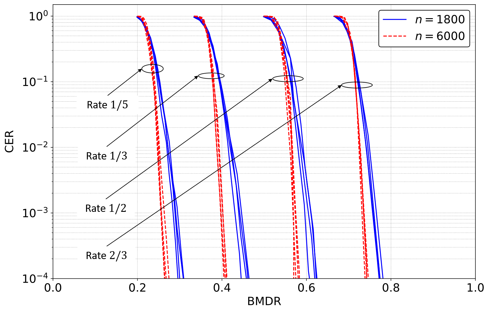
Figure 2: BMDR vs CER for the SISO-AWGN channel using $4/16/64/256-$QAM and different code-rates. The solid blue lines correspond to a length-$1800$ 5G-LDPC code while the dashed red lines correspond to a length-$6000$ 5G-LDPC code.

Before detailing the algorithm for LA, it is necessary to describe a method to map BMDR to CER. Fig. 2 shows the plots of the CER as a function of BMDR for the SISO-AWGN channel with the MLD, for length-$1800$ and length-$6000$ 5G-low-density parity-check (LDPC) codes of various rates. The plots were numerically obtained for $4/16/64/256-$QAM (with the smaller constellation slightly better than the larger constellation). For each modulation order, we chose a range of signal-to-noise ratio (SNR) values, and computed the CER of a particular length-$n$, rate-$r$ LDPC code for a set of uniformly spaced SNR values within the chosen range. We then empirically computed the BMDR for the same modulation order and for the same set of chosen SNR values. After numerically obtaining the BMDR-CER pair for each SNR value, we plotted CER as function of BMDR for each code and modulation order. It is to be noted that since we are using the MLD, for any SNR value, the corresponding BMDR multiplied by $m$ is the capacity of BICM for $2^{m}$-QAM [16] at that SNR. Therefore, even though the BMDR curves for the same value of $n$ and $r$ and for different modulation orders nearly coincide, the overall capacity of the system is $m$ times the BMDR for any particular modulation order $m$. To illustrate further with an example, let us consider the rate-$1/3$ channel coding scheme with codeword length $n=1800$ and modulation orders $2$ and $4$ (corresponding to QPSK and $16$-QAM). For a target CER of $10^{-3}$, the corresponding BMDR for both the modulation orders is approximately $0.45$. This means that while a CER of $10^{-3}$ was observed for QPSK at a certain SNR $\rho_{a}$ and that for $16$-QAM at a different SNR $\rho_{b}$ (with $\rho_{b}>\rho_{a}$), the observed BMDR with QPSK at an SNR of $\rho_{a}$ was the same as the observed BMDR with $16$-QAM at an SNR of $\rho_{b}$. It is also to be noted that with $16$-QAM, the number of transmitted coded bits per channel use is twice that with QPSK, albeit at a higher SNR, in order to achieve the same CER. The other important observation from the plots is that the same target CER can be achieved with lower BMDR by increasing the codeword length $n$. These observations suggest that for a given code-rate, BMDR is strongly dependent on the codeword length and weakly dependent on the modulation order.

We propose to generate a lookup table using simulations performed on a SISO AWGN channel. We expect this lookup table to be relevant even to the case of MU-MIMO because the proof of [1, Theorem 1] suggests that the error behavior of a coding scheme depends predominantly on BMDR alone. In the rest of the paper, to distinguish between codes from the same family (like the 5G-LDPC codes), we explicitly state the rate and length; so ${\mathcal{C}}(r,n)$ denotes a code with rate $r$ and length $n$. Let $\mathzapf{R}\left(m,{\mathcal{C}}(r,n),\epsilon\right)$ denote the target BMDR required to be guaranteed of a CER of at most $\epsilon$ for the SISO-AWGN channel using $2^{m}$-QAM, ${\mathcal{C}}(r,n)$, and the MLD. With this, for a low target probability of codeword error $\epsilon$ ($<10^{-1}$), we can expect the following.

1. $\mathzapf{R}\left(m,{\mathcal{C}}(r,n_{1}),\epsilon\right)\leq\mathzapf{R}\left(m,{\mathcal{C}}(r,n_{2}),\epsilon\right)$ if $n_{1}>n_{2}$.

2. $\mathzapf{R}\left(m_{1},{\mathcal{C}}(r,n),\epsilon\right)\approx\mathzapf{R}\left(m_{2},{\mathcal{C}}(r,n),\epsilon\right)$ if $m_{1}\neq m_{2}$.

Algorithm 1 Pseudocode to generate a look-up table that maps AWGN BMDR to CER.

Input

     ${\mathcal{C}}(r,n)$: Channel code with code-rate $r$ and length $n$

     $m$: Modulation order used, implies $2^{m}$-QAM

     $\mathfrak{P}$: Discrete set of usable SNR values in $\mathrm{dB}$,

               $\mathfrak{P}=\left\{\rho_{min}+l\Delta\rho,~{}l=0,1,\cdots,\left\lfloor\frac{\rho_{max}-\rho_{min}}{\Delta\rho}\right\rfloor\right\}$

Output

     ${\cal L}_{U}$: Look-up table containing BMDR-CER pairs

Initialize

      ${\cal L}_{U}\leftarrow\left\{\right\}$

for all $\rho\in\mathfrak{P}$ do

     /* Empirically compute CER for SISO-AWGN channel with channel code ${\mathcal{C}}(r,n)$,

        $2^{m}$-QAM, and maximum-likelihood detection at an SNR of $\rho$ $\mathrm{dB}$ */

     $P_{e}\leftarrow\mathrm{CER}\Big{(}$SISO-AWGN, $2^{m}$-QAM, ${\mathcal{C}}(r,n)$, $\rho\Big{)}$

     /* Empirically compute BMDR for SISO-AWGN channel with $2^{m}$-QAM and

       maximum-likelihood detection at an SNR of $\rho$ $\mathrm{dB}$ */

     $R_{MLD}\leftarrow\mathrm{BMDR}\Big{(}$SISO-AWGN, $2^{m}$-QAM, $\rho\Big{)}$

     ${\cal L}_{U}\leftarrow{\cal L}_{U}\cup\left\{\left(R_{MLD},P_{e}\right)\right\}$

end for

Algorithm 1 provides pseudocode for the lookup table generation technique. In the algorithm, BMDR is empirically calculated using the method outlined in [1, Algorithm 1], but for a SISO-AWGN channel. Since the effect of QAM size on the target BMDR appears to be very small, one can use just QPSK in Algorithm 1 instead of higher dimensional $2^{m}$-QAM in order to reduce the computational complexity. Having generated the lookup table ${\cal L}_{U}$ as detailed in Algorithm 1, $\mathzapf{R}\left(m,{\mathcal{C}}(r,n),\epsilon\right)$ for a target CER of $\epsilon$ can be obtained from ${\cal L}_{U}$ as

$$\mathzapf{R}\left(m,{\mathcal{C}}(r,n),\epsilon\right)=\min_{\left(R_{MLD},P_{e}\right)\in{\cal L}_{U}}\left\{R_{MLD}~{}|~{}P_{e}\leq\epsilon\right\}.$$ (7)

It is common to have several choices for the code-length $n$ for a given code-rate $r$. For example, in 5G NR, $k\in\{1,8448\}$ [12, Section 5] so that $1/r\leq n\leq 8448/r$. It would be practically infeasible to generate a lookup table for each combination of $n$ and $r$. Instead, one can compute $\mathzapf{R}\left(m,{\mathcal{C}}(r,n),\epsilon\right)$ for a few values of $n\in[n_{min},n_{max}]$ (extremes included), where $n_{max}$ and $n_{min}$ denote the maximum and minimum code-lengths, respectively. From these computed values, any target BMDR for intermediate lengths ($n_{min}<n<n_{max}$) can be estimated by linear or polynomial interpolation. We do not go into the details of this and assume that for any target CER $\epsilon$, code-rate $r$, modulation order $m$, and code-length $n_{min}\leq n\leq n_{max}$, there exists a (possibly learned) function $\mathzapf{R}$ which outputs the estimated target BMDR for ${\mathcal{C}}(r,n)$ with $2^{m}$-QAM.

IV Link-Adaptation in MU-MIMO Systems

Let ${\cal M}$ denote the set of available modulation orders, and ${\cal R}(m)$ denote the set of available code-rates for $m\in{\cal M}$. We also assume for the sake of simplicity that the codewords of all the users are to be transmitted over the same set of REs with the corresponding set of channel realizations denoted by ${\cal H}_{next}$. This means that if UE $i$ selects a modulation order $m_{i}$, the code-length of the channel code that it uses is $|{\cal H}_{next}|m_{i}n_{t}^{(i)}$. Assuming the usage of an arbitrary detector ${\cal D}$ and a target CER of $\underline{\epsilon}$ for all users, MCS selection aims to solve the following joint spectral efficiency (SE)-maximizing problem.

$$\left\{\left(m_{i}^{*},r_{i}^{*}\right)\right\}_{i=1}^{N_{u}}=\underset{\left\{m_{i}\in{\cal M},r_{i}\in{\cal R}(m_{i})\right\}_{i=1}^{N_{u}}}{\operatorname{arg}\,\operatorname{max}}\;\left\{\frac{1}{N_{u}}\sum_{i=1}^{N_{u}}r_{i}m_{i}~{}\Big{|}~{}R_{{\cal D},i}\left(\mathfrak{m},{\cal H}_{next}\right)\geq\mathzapf{R}\left(m_{i},{\mathcal{C}}(r_{i},n_{i}),\underline{\epsilon}\right)\right\}$$ (8)

where $\mathfrak{m}=\left\{m_{1},\cdots,m_{N_{u}}\right\}$. However, we do not yet have the estimates of the channel matrices of ${\cal H}_{next}$, and can only rely on the most recent past-channel estimates. In 5G NR, these can be the channel estimates obtained using demodulation reference signals (DMRSs) in the previous transmission slot for those users that have already transmitted, or using sounding reference signals (SRSs) if there was no transmission in the previous slot. We denote the set of these channel estimates by $\widehat{{\cal H}}$. Using a trained BMDR-predictor [1, Section V], the BMDR for UE $i$ can be predicted for $\widehat{{\cal H}}$ as $\hat{R}_{{\cal D},i}\left(\mathfrak{m},\widehat{{\cal H}}\right)$. However, since these are estimates on a possibly outdated set of channel estimates, we need a BMDR-correction offset $\delta_{i}$ for each UE $i$. This correction offset is similar to the SINR-correction offset in OLLA, and it captures the amount of confidence one has in the estimated BMDR; the greater the confidence, the closer $\delta_{i}$ is to $0$. In case the BMDR is underestimated, a positive $\delta_{i}$ acts as a correction. In large file transfers, $\delta_{i}$ typically varies throughout the transmission; decreasing by a large value for every incorrectly decoded codeword, and increasing by a small value otherwise. With this, the practical MCS-selection problem can be restated as

$$\left\{\left(m_{i}^{*},r_{i}^{*}\right)\right\}_{i=1}^{N_{u}}=\underset{\left\{m_{i}\in{\cal M},r_{i}\in{\cal R}(m_{i})\right\}_{i=1}^{N_{u}}}{\operatorname{arg}\,\operatorname{max}}\;\left\{\frac{1}{N_{u}}\sum_{i=1}^{N_{u}}r_{i}m_{i}~{}\Big{|}~{}\hat{R}_{{\cal D},i}\left(\mathfrak{m},\widehat{{\cal H}}\right)\geq\mathzapf{R}\left(m_{i},{\mathcal{C}}(r_{i},n_{i}),\underline{\epsilon}\right)-\delta_{i}\right\}.$$ (9)

In general, the worst case complexity of an algorithm that solves (9) using brute-force search is ${\cal O}\left(n_{MCS}^{N_{u}}\right)$, where $n_{MCS}$ is the number of available MCS levels. But, if the detector ${\cal D}$ were such that for any $i\in\left\{1,\cdots,N_{u}\right\}$,

$$\hat{R}_{{\cal D},j}\left(\mathfrak{m},\mathrm{H}\right)=\hat{R}_{{\cal D},j}\left(\mathfrak{m}^{\prime},\mathrm{H}\right),\forall j\neq i$$ (10)

where $\mathfrak{m}$ and $\mathfrak{m}^{\prime}$ only differ in modulation order for UE $i$. In other words, if the detector is such that when the constellation of one UE is changed and those of the others are kept the same, only the BMDR of that particular UE changes while those of the other users are unaffected, it is possible to solve (9) efficiently with much lower complexity. Algorithm 2 provides pseudocode to do so for such detectors. In the algorithm, when calculating $r_{i}^{*}$ for a chosen $m_{i}^{*}$, if there is no $r_{i}\in{\cal R}(m_{i}^{*})$ satisfying $\hat{R}_{{\cal D},i}\left(\mathfrak{m},\widehat{{\cal H}}\right)\geq\mathzapf{R}\left(m_{i}^{*},{\mathcal{C}}(r_{i},n_{i}),\underline{\epsilon}\right)-\delta_{i}$, we choose $r_{i}^{*}=\min{\cal R}(m_{i}^{*})$. The worst case complexity of Algorithm 2 is ${\cal O}\left(N_{u}n_{MCS}\right)$ which is incurred when the for-loop is fully executed, i.e., for each UE $i$, $c_{i}$ is updated sequentially from $k_{max}$ to $1$. This would essentially have tested the BMDR criterion for each MCS level for each UE. For linear detectors, BMDR is a non-decreasing function of the post-equalization SINR [1] which is unaffected for a user by a change of constellation for any other user, provided that all constellations have unit energy. Our numerical studies seem to indicate that (10) holds for the $K$-best detector as well. In general, Algorithm 2 might be suboptimal for arbitrary non-linear detectors, but still is a low-complexity alternative to any other optimal algorithm with higher complexity.

Algorithm 2 Pseudocode to select MCS for each user based on channel measurements.

Input

     ${\cal M}$: Set of available QAM modulation orders, ${\cal M}=\{2k,k=1,\cdots,k_{max}\}$

     $\mathcal{R}(m)$: Set of available code-rates for modulation order $m$, $\forall m\in{\cal M}$

     $\mathzapf{R}$: Learned function to predict the target BMDR for a target CER $\underline{\epsilon}$ given

               code-rate $r$, code-length $n$, modulation order $m$

     $\delta_{i}$: Precomputed BMDR-correction offset for UE $i$, $\forall i=1,\cdots,N_{u}$

     $\widehat{{\cal H}}$: Set of estimated composite MU-MIMO channel matrices of size $n_{r}\times N$

     $n_{RE}$: Number of REs for codeword transmission

     $f_{{\cal D},i}$: A pretrained BMDR-predictor for detector ${\cal D}$ and UE $i$, $\forall i=1,\cdots,N_{u}$,

               takes as inputs the channel matrix and set of modulation orders for all users

Output

     $mcs_{i}$: Chosen MCS index for UE $i$, $\forall i=1,\cdots,N_{u}$

Initialize

      $\mathrm{updateFlag}\leftarrow\mathrm{True}$ $c_{i}\leftarrow k_{max}$, $\forall i=1,\cdots,N_{u}$ $\triangleright$ Begin with the highest modulation order

while $\mathrm{updateFlag}$ is $\mathrm{True}$ do

     $m_{i}\leftarrow 2c_{i}$, $n_{i}\leftarrow n_{RE}m_{i}n_{t}^{(i)}$, $\forall i=1,\cdots,N_{u}$ $\triangleright$ Assign modulation order to user

     $\mathfrak{m}\leftarrow\{m_{1},\cdots,m_{N_{u}}\}$

     $\hat{R}_{{\cal D},i}\left(\mathfrak{m},\widehat{{\cal H}}\right)\leftarrow\frac{1}{\left|\widehat{{\cal H}}\right|}\sum_{\widehat{\mathbf{H}}\in\widehat{{\cal H}}}f_{{\cal D},i}\left(\mathfrak{m},\widehat{\mathbf{H}}\right)$, $\forall i=1,\cdots,N_{u}$ $\triangleright$ Estimate average BMDR

     for all $i=1,\cdots,N_{u}$ do

         if $\hat{R}_{{\cal D},i}\left(\mathfrak{m},\widehat{{\cal H}}\right)<\min_{r_{i}\in{\cal R}(m_{i})}\left\{\mathzapf{R}\left(m_{i},{\mathcal{C}}(r_{i},n_{i}),\underline{\epsilon}\right)\right\}-\delta_{i}$ then $\triangleright$ BMDR criterion

              $c_{i,next}\leftarrow\max(c_{i}-1,1)$ $\triangleright$ Reduce modulation order

         end if

     end for

     if $c_{i,next}=c_{i}$, $\forall i=1,\cdots,N_{u}$ then

         $\mathrm{updateFlag}\leftarrow\mathrm{False}$ $\triangleright$ No more updates of modulation orders

     end if

     $c_{i}\leftarrow c_{i,next}$, $\forall i=1,\cdots,N_{u}$

end while

$m_{i}^{*}\leftarrow m_{i},~{}~{}r_{i}^{*}\leftarrow\underset{r_{i}\in\mathcal{R}(m_{i})}{\operatorname{arg}\,\operatorname{max}}\;\left\{\hat{R}_{{\cal D},i}\left(\mathfrak{m},\widehat{{\cal H}}\right)\geq\mathzapf{R}\left(m_{i},{\mathcal{C}}(r_{i},n_{i}),\underline{\epsilon}\right)-\delta_{i}\right\}$, $\forall i=1,\cdots,N_{u}$

$mcs_{i}\leftarrow\mathrm{MCS}(m_{i}^{*},r_{i}^{*})$, $\forall i=1,\cdots,N_{u}$ $\triangleright$ Map $(m_{i}^{*},r_{i}^{*})$ to MCS index

IV-A Dynamic Detector Selection

Suppose that there are $N_{d}$ available detectors $\left\{{\cal D}_{p}\right\}_{p=1}^{N_{d}}$ to choose from, with the complexity of ${\cal D}_{p}$ denoted by $\mathfrak{C}({\cal D}_{p})$. We emphasize here that the complexity could either be in terms of time taken to perform detection for one RE, or in terms of the number of computations performed during the course of detection for one RE. The two need not be proportional to one another, an example being the case where a particular detector performs more operations than its rival but allows parallel processing while its rival does not. Depending on the application, the complexity metric is chosen such that a less "complex" detector is more desirable for usage than its rival if both the detectors are equally reliable. The list of detectors $\{{\cal D}_{1},\cdots,{\cal D}_{N_{d}}\}$ is assumed to be ordered so that $\mathfrak{C}({\cal D}_{1})\leq\cdots\leq\mathfrak{C}({\cal D}_{N_{d}})$. The goal is to choose the least complexity detector that can meet certain target metrics (like throughput or error rates).

This problem has been considered in various settings in the literature. In [17], the authors consider a single user $2\times 2$ and $4\times 4$ MIMO system and compare the performances of three detectors: the LMMSE detector, soft interference cancellation (SIC), and the $K$-best detector. Through experiments, they recommend the usage of the LMMSE detector at low SINR and the $K$-best at high SINR. In [18], an asymptotic bit error rate (BER) analysis is performed to obtain SINR thresholds that allow detector switching between SIC and $K$-best detection. The problem of adaptively allocating computational resources to the detection problem for each channel realization, under a total per codeword complexity constraint, is considered in [19]. Placing the MLD on one end of the spectrum and the zero-forcing (ZF) detector at the other end, the paper considers the mutual-information (MI) of the MIMO channel for a Gaussian-distributed input to be the metric for the MLD and a similarly calculated MI to be the corresponding metric for the ZF detector, and proposes a linear interpolation between these two metrics as the metric for any detector with intermediate computational complexity. Since practical communication systems use QAM constellations, the MI for a Gaussian-distributed input is not the ideal choice of metric. Moreover, the aforementioned linear interpolation is not known to be accurate in general. A neural network (NN)-based approach to switch between detectors in each RE of an OFDM-based MIMO system is presented in [20] while a reinforcement-learning (RL)-based approach is considered in [21]. The limitation of all these works is that the proposed techniques cannot be extended to a MU-MIMO setting where different UEs can have different MCS levels.

Let $m_{{\cal D}_{p},i}^{*}$ and $r_{{\cal D}_{p},i}^{*}$ respectively denote the estimated modulation order and code-rate for UE $i$ with detector ${\cal D}_{p}$ according to Algorithm 2. Then, one can use a hybrid detection strategy that dynamically chooses ${\cal D}_{p^{*}}$ where

$$p^{*} =\min\left\{\underset{p\in\{1,\cdots,N_{d}\}}{\operatorname{arg}\,\operatorname{max}}\;\left\{\frac{1}{N_{u}}\sum_{i=1}^{N_{u}}r_{{\cal D}_{p},i}^{*}m_{{\cal D}_{p},i}^{*}\right\}\right\}.$$ (11)

In other words, (11) attempts to choose the least complexity detector among the ones that offer the best average SE subject to a target CER constraint for each user. This is a more natural way of selecting a detector in an MU-MIMO setting with LA compared to the existing works in the literature. Another possible detector selection strategy is to choose ${\cal D}_{p^{*}}$ with

$$p^{*} =\underset{p\in\{1,\cdots,N_{d}\}}{\operatorname{arg}\,\operatorname{max}}\;\left\{\gamma f_{1}({\cal D}_{p})+(1-\gamma)f_{2}({\cal D}_{p})\right\},$$ (12)

where $\gamma\in\left[0,1\right]$, $f_{1}({\cal D}_{p})\triangleq(1/(N_{u}r_{max}m_{max}))\sum_{i=1}^{N_{u}}r_{{\cal D}_{p},i}^{*}m_{{\cal D}_{p},i}^{*}$, and $f_{2}({\cal D}_{p})\triangleq-\mathfrak{C}({\cal D}_{p})/\mathfrak{C}({\cal D}_{N_{u}})$. Here, $r_{max}m_{max}$ denotes the SE corresponding to the highest available MCS level. By varying the value of the weight $\gamma$, (12) helps obtain a balance between SE and computational complexity. A value of $\gamma$ closer to $1$ puts more emphasis on maximizing the SE while a value closer to $0$ puts more emphasis on choosing the least complexity detector.

V Physical Layer Abstraction

With the system model as described in Section II, assume that UE $i$ transmits the codeword bits on $n_{RE}$ REs, each RE indexed by the frequency-time pair $(f,t)$. Let ${\cal G}_{i}$ denote the set of index pairs with the associated set of channel realizations ${\cal H}_{{\cal G}_{i}}=\left\{\mathrm{H}_{f,t},(f,t)\in{\cal G}_{i}\right\}$. Assuming a linear receiver, the crucial step in PHY abstraction in the literature [13, 14, 15] is to obtain an effective SINR $\bar{\rho}_{i}$ as follows.

$$\bar{\rho}_{i}=\beta_{1}I^{-1}\left(\frac{1}{n_{RE}}\sum_{(f,t)\in{\cal G}_{i}}I\left(\frac{\rho_{f,t,i}}{\beta_{2}}\right)\right)$$ (13)

where $I()$ is a model-specific function, $\rho_{f,t,i}$ is the post-equalization SINR for UE $i$ in the RE indexed by $(f,t)$, and $\beta_{1},\beta_{2}$ are parameters that allow the model to adapt to the characteristics of the considered MCS. CESM corresponds to $I(x)=\mathop{\mathrm{log}_{2}}\left(1+x\right)$, EESM to $I(x)=e^{-x}$, LESM to $I(x)=\mathrm{log}_{10}(x)$, and MIESM to $I(x)={\cal I}_{m}(x)$ where ${\cal I}_{m}(x)$ refers to the MI between the input and the output in an AWGN channel with $2^{m}$-QAM and an SNR of $x$. Following the computation of this effective SINR, a SINR-CER mapping is performed to obtain the error metrics. Currently, there is no clear consensus on which model-specific function to use, and more importantly, on how to use the above technique for non-linear receivers.

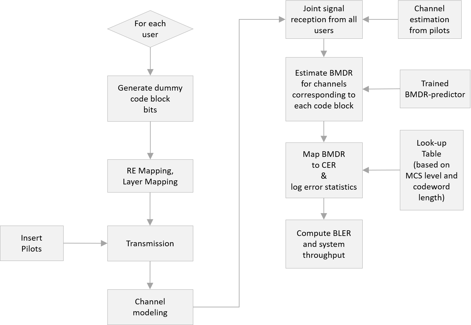
Figure 3: Flowchart of the proposed PHY abstraction with the time-intensive procedures of Fig. 1 replaced by less complex procedures.

BMDR serves as a more natural metric for performing PHY abstraction. This is because the BMDR-CER relationship is clearer than the ESM-CER relationship, where the effective SINR is calculated using (13). We note that while BMDR is equivalent to MIESM for linear receivers, it can be applied to non-linear receivers as well. Our proposed approach is to calculate

$$\hat{R}_{{\cal D},i}\left(\mathfrak{m},{\cal H}_{{\cal G}_{i}}\right)=\frac{1}{n_{RE}}\sum_{(f,t)\in{\cal G}_{i}}\hat{R}_{{\cal D},i}\left(\mathfrak{m},\mathrm{H}_{f,t}\right)$$ (14)

where $\mathfrak{m}=\left\{m_{1},\cdots,m_{N_{u}}\right\}$ is the set of modulation orders used by all the co-scheduled users, and then map $\hat{R}_{{\cal D},i}\left(\mathfrak{m},{\cal H}_{{\cal G}_{i}}\right)$ to a CER using the lookup table ${\cal L}_{U}$ whose construction was detailed in Section III. With respect to 5G NR terminology [12], suppose that UE $i$ notionally transmits $B$ transport-blocks (TBs), with each TB being segmented into $L$ CBs (a CB is a block of message bits). Therefore, a total of $BL$ codewords are transmitted notionally (not actually transmitted because of the abstraction model). Then, the BMDR associated with each codeword transmission is estimated and mapped to a CER value from the lookup table. Let the estimated BMDR associated with the $l^{th}$ codeword of TB $j$ be $\hat{R}^{(j,l)}_{{\cal D},i}\left(\mathfrak{m},{\cal H}_{{\cal G}_{i}}^{(j,l)}\right)$ where ${\cal H}_{{\cal G}_{i}}^{(j,l)}$ is the associated set of channel realizations, and let $\hat{p}_{i,j,l}$ denote the estimated CER for this codeword. Then,

$$\hat{p}_{i,j,l}=\underset{P_{e}(R_{MLD})\in{\cal L}_{U}}{\operatorname{arg}\,\operatorname{min}}\;\left\{\left|R_{MLD}-\hat{R}^{(j,l)}_{{\cal D},i}\left(\mathfrak{m},{\cal H}_{{\cal G}_{i}}^{(j,l)}\right)\right|\right\}$$ (15)

and the estimated probability of error for TB $j$ is $\hat{P}_{i,j}=1-\prod_{l=1}^{L}\left(1-\hat{p}_{i,j,l}\right)$. The overall BLER for UE $i$ is $\frac{1}{B}\sum_{j=1}^{B}\hat{P}_{i,j}$. The average system throughput can be estimated from the BLERs of all the users. Fig. 3 shows the flowchart of the proposed technique.

VI Simulation Results

VI-A Simulation Setup

Parameter	Value
$N_{u}$	$4$
$n_{t}^{(i)}$	$1$, $\forall i=1,\cdots,4$
$n_{r}$	$16$ ($2$H$\times 8$V)
Number of cells in grid	$21$
Total number of users in grid	$210$
Inter-site distance	$200\text{\,}\mathrm{m}$
Channel model	38.901 Urban Micro (UMi) NLoS
Carrier frequency	$3.5\text{\,}\mathrm{GHz}$
OFDM subcarrier spacing	$30\text{\,}\mathrm{kHz}$
System bandwidth	$8.64\text{\,}\mathrm{MHz}$
Number of OFDM symbols/slot	$14$
OFDM symbol duration	$35.7\text{\,}\mathrm{\SIUnitSymbolMicro s}$
Number of PRBs/slot	$24$
UE speed	$5\text{\,}\mathrm{kmph}$
UE max transmit power $P_{max}$	$23\text{\,}\mathrm{dBm}$
UE uplink power control $(P_{0},\alpha)$	($-98\text{\,}\mathrm{dBm}$, $0.7$), ($-98\text{\,}\mathrm{dBm}$, $1$)

TABLE III: A list of simulation parameters.

We consider the following setup (with a summary of the parameters in Table III) for performing multi-cell, multi-link-level simulations, the code for which was written in NumPy (for channel generation) and TensorFlow. We consider 7 sites with 3 cells per site, leading to a total of $21$ cells arranged in a hexagonal grid with wraparound (which essentially means that each cell sees an inter-cell interference pattern similar to that of the central cell). The inter-site distance is $200\text{\,}\mathrm{m}$, and we consider the 38.901 Urban Micro (UMi) NLoS [22, Section 7.2] channel model. A total of $210$ users are dropped at random in this grid. The carrier frequency is $3.5\text{\,}\mathrm{GHz}$ and each BS is equipped with a rectangular planar array consisting of $16$ ($2$ vertical, $8$ horizontal) single-polarized antennas installed at a height of $25\text{\,}\mathrm{m}$ and an antenna spacing of $0.5\lambda$, where $\lambda$ is the carrier wavelength. The UEs are each equipped with $2$ dual-polarized antennas ($1$ vertical, $2$ horizontal), and the maximum total output power $P_{max}$ per UE is $23\text{\,}\mathrm{dBm}$. We consider a regular 5G OFDM grid with a subcarrier spacing of $30\text{\,}\mathrm{kHz}$, a slot of $14$ symbols (of duration $35.7\text{\,}\mathrm{\SIUnitSymbolMicro s}$ each), and $24$ PRBs (of $12$ subcarriers each) leading to a total usable system bandwidth of $8.64\text{\,}\mathrm{MHz}$. Out of the $14$ symbols, four are used for DMRS transmission and the remaining for data. The total uplink transmit power $\rho$ (in dBm) used by each UE is given by the following open-loop-power-control (OLPC) equation [23, Section 7]:

$$\rho=\min\{P_{max},P_{0}+10\mathop{\mathrm{log}_{10}}\left(N_{PRB}\right)+\alpha PL\}$$ (16)

where $P_{max}=23$, $N_{PRB}=24$ is the total number of PRBs, $PL$ is the pathloss estimate (based on the measured channel gains on the downlink), $P_{0}$ is the expected received power per PRB under full pathloss compensation, and $\alpha\in[0,1]$ is the fractional pathloss compensation factor. In our simulations, we take $P_{0}$ to be $-98\text{\,}\mathrm{dBm}$ and $\alpha\in\{0.7,1\}$. The transmission of each codeword is completed within each slot, so we fix the codeword length to be $2880$ for all MCS levels. A custom MCS table as shown in Fig. 4 is used, where $m$ refers to the modulation order, $k$ to the message length, $n$ to the codeword length, and $\textrm{SE}=mk/n$. 5G LDPC codes are used for channel coding.

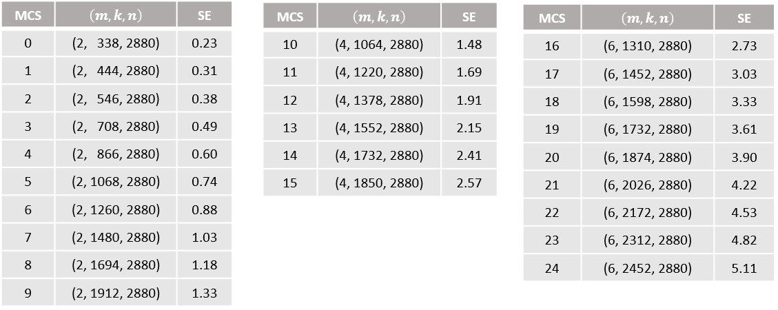
Figure 4: The MCS table used for simulations.

Once the users are dropped, they are assumed to have a speed of $5\text{\,}\mathrm{kmph}$, and the simulations are evaluated for $500$ slots (of $0.5\text{\,}\mathrm{ms}$ each). The metrics are evaluated for ten such independent user drops. The number of transmitting layers is fixed to be four; so, depending on the users’ positions, a single user can transmit using all of its four antennas, or four users can transmit using a single antenna each (and any combination of user antennas summing to four). The users are scheduled as follows: for each user, its serving cell is identified to be the one for which the average channel gains are the highest. Next, the $n_{r}\times n_{r}$ sized channel covariance matrix for each user is estimated at the BS using the SRS signals sent by the user, and is calculated by averaging over both time and frequency. Then, the set of users in each cell is divided into (not disjoint) subsets such that in each subset, the cross-correlation between the principal eigenvectors of the channel covariance matrices of any two users is less than $0.1$. The cardinality of each subset is limited to four, and the subsets are served in a round-robin fashion. LMMSE channel estimation is performed for each user, and the interference covariance matrix at each cell is assumed to be perfectly known (i.e., with the notation as used in Section II, $\mathbf{K}_{n}$ is assumed to be perfectly known while $\mathbf{K}_{e}$ is estimated).

The BMDR-CER map is generated as explained in Section III using $100,000$ codewords for each SNR, and the BMDR is computed using $10,000$ independent input symbol and noise realizations for the same SNR in order to do the Monte-Carlo approximation of (6) for the SISO-AWGN channel.

For LLR generation, we consider the LMMSE detector as our choice of linear detector, and the $32$-best detector ($K=32$ in [7]) as our choice of non-linear detector. Their respective BMDR-predictors are trained as explained in [1, Section V]. We would like to reiterate that the reason for choosing the $32$-best detector is due to its relatively low complexity compared to other non-linear techniques. In practice, it is often required to go beyond $K=64$ in order to achieve significant performance gains over LMMSE. The purpose of our simulations is not to show that one detector is superior to the other, but rather to corroborate our claims about the role of BMDR in LA and PHY abstraction for both linear and non-linear detectors.

The throughput for each user in a given user drop, when using a particular detector, is obtained as follows: Suppose that UE $i$ transmits a total of $L_{i}$ codewords in that drop, with the $j^{th}$ codeword carrying $k_{ij}$ message bits. Let the total number of slots for that drop be $T$, with each slot being of duration $t_{slot}$ seconds. Let $\delta_{ij}=1$ if the $j^{th}$ codeword is correctly decoded using the LDPC decoder for which the input LLRs are generated by the detector in context, and $0$ otherwise. We do not consider any type of automatic repeat request (ARQ) in our simulations. Then, the throughput $TP_{i}$ in megabits per second (Mbps) for UE $i$ in that user drop is

$$TP_{i}=\frac{1}{10^{6}}\left(\frac{\sum_{j=1}^{L_{i}}\delta_{ij}k_{ij}}{Tt_{slot}}\right).$$ (17)

The arithmetic mean (AM) and the geometric mean (GM) of the throughputs for all the users in a drop are then recorded, and this process is repeated for each of the ten independent drops. While the throughput for each user is heavily dependent on the user-scheduling algorithm, the goal here is to assess the performance of the detectors considered.

VI-B LA: Numerical Results

For MCS selection, we use the previous slot’s channel realizations even if the users didn’t transmit, except for the first slot in which case we estimate the first slot’s channels before selecting the MCS. We choose a target CER of $10^{-3}$. With this setup, we simulate the following four receiver algorithms:

1. LMMSE detection with EESM-based MCS selection: In this case, we use the LMMSE detector and use EESM for MCS estimation. To be precise, we compute the post-equalization SINR for each user in each PRB using the previous slot’s channel realizations. Let $\hat{\rho}_{i,n}$ denote the post-equalization SINR for UE $i$ in the $n^{th}$ PRB, $n=1,\cdots,24$. The effective SINR $\bar{\rho}_{i}$ is estimated to be [24]

   $$\bar{\rho}_{i}=-\beta\mathop{\mathrm{ln}}\left(\frac{1}{24}\sum_{n=1}^{24}\mathop{\mathrm{exp}}\left(-\frac{\hat{\rho}_{i,n}}{\beta}\right)\right)$$ (18)

   where the value of $\beta$ is chosen according to [24, Table II] for each available MCS. Finally, the highest MCS that meets the target CER is selected using an SNR-CER map. We call this scheme “LMMSE-EESM".

2. LMMSE detection with BMDR-based MCS selection: This uses the LMMSE detector with the MCS selected according to Algorithm 2. This scheme is called “LMMSE-BMDR".

3. $32$-best detection with BMDR-based MCS selection: This scheme uses the $32$-best detector and Algorithm 2, and is called “$32$-best-BMDR”.

4. Hybrid detector: selects either the LMMSE detector or the $32$-best detector in each slot according to (11), and is called “Hybrid-BMDR".

We have considered the EESM-based effective SINR mapping because it is the one recommended by 3GPP. We did not explicitly simulate the RBIR-based effective SINR mapping scheme (which is a variant of the MIESM-based mapping and is proposed for usage in IEEE 802.11) because, for linear detectors, this turns out to be equivalent to our proposed BMDR-based approach. Since there is no known effective SINR mapping scheme for non-linear detectors, we have only considered the proposed BMDR-based approach for the $32$-best detector.

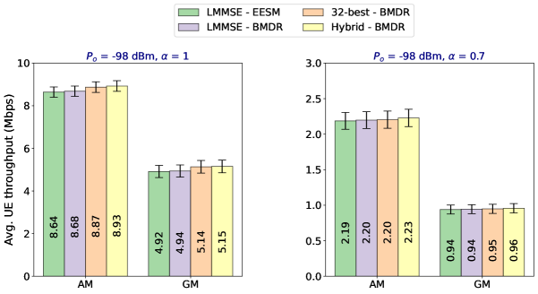
Figure 5: The AM and GM throughputs with $90\%$ confidence intervals for the four detection schemes for (left) $\alpha=1$ and (right) $\alpha=0.7$.

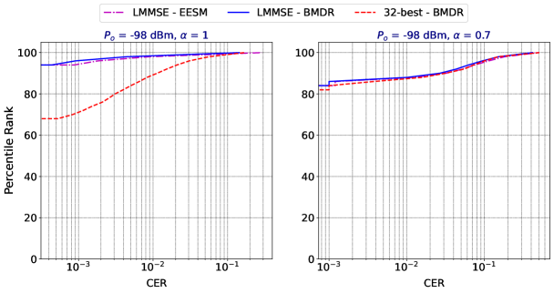
Figure 6: The percentiles of the CER for the LMMSE detector and the $32$-best detector for (left) $\alpha=1$ and (right) $\alpha=0.7$. For any CER value $p_{e}$ on the X-axis, the corresponding value on the Y-axis indicates the percentage of users (across all drops) that achieved a CER $\leq p_{e}$.

Figure 7: The percentiles of the MCS levels for the LMMSE detector and the $32$-best detector for (left) $\alpha=1$ and (right) $\alpha=0.7$.

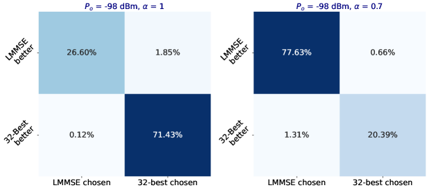
Figure 8: The confusion matrix for detector selection using the proposed technique for (left) $\alpha=1$ and (right) $\alpha=0.7$.

Fig. 5 shows the plots of the average AM and GM throughputs for the four schemes along with the $90\%$ confidence intervals (for different user drops). Fig. 6 shows the percentiles of the CER for the LMMSE detector (both EESM-based and BMDR-based) and the $32$-best detector, so that for each CER value $p_{e}$ on the X-axis, the corresponding value on the Y-axis indicates the percentage of users (across all drops) that achieved a CER less than or equal to $p_{e}$. Fig. 7 shows the percentiles of the MCS levels selected by the different schemes.

It can be seen from Fig. 5 that the hybrid detector gives the best performance, while LMMSE-EESM and LMMSE-BMDR have nearly the same performance. This is not surprising, given that both EESM and MIESM have been thoroughly evaluated in the literature to provide near-optimal performance, and the proposed BMDR-based approach for LMMSE detection is equivalent to the MIESM-based approach. From Fig. 6, it can be seen that for the case of $\alpha=1$ (full path-loss compensation), users achieve the target CER of $10^{-3}$ with LMMSE detection (both EESM-based and BMDR-based) around $94\%$ of the time while this number is $68\%$ for the $32$-best detector. The reason for this difference, as highlighted in [1], is the ability to perform more accurate BMDR-prediction for a linear detector than for a non-linear detector, and is down to the accuracy of the trained BMDR-predictors. For the case of $\alpha=0.7$ (with partial path-loss compensation), the percentage of the time the CER target is met is around $82\%$ for both the detectors. This is due to an increase in the usage of the lowest available MCS, as observed in Fig. 7. Since the path-loss is not fully compensated, it might be that some users might not have sufficient SINR for error-free transmission even at the lowest MCS level. From Fig. 7, it can be readily seen that the users experience a wide range of MCS values for all detection schemes, and depending on the path-loss compensation factor, have a bias towards either the lower MCS levels ($\alpha=0.7$) or the higher ones ($\alpha=1$). For the case of $\alpha=1$, the plots for the LMMSE detector with EESM-based and BMDR-based mapping coincide, and the $32$-best detector allows slightly higher MCS selection, evidenced by its curve being below that of the LMMSE detector.

Fig. 8 shows the confusion matrices of the detector selection algorithm which corroborates the efficacy of the proposed method. Since the $32$-best detector uses only $32$ survivors per layer in the search tree, there are scenarios where the LLRs might be overestimated due to the lack of a sufficient number of candidates of the opposite polarity for each transmitted bit. This leads to poorer performance compared to LMMSE in such cases. Therefore, depending on the channel conditions, the hybrid detection scheme allows us to use a combination of a low-complexity detector and higher complexity non-linear detector for an overall better performance. To summarize, the main inferences from Figs. 5–8 are:

1. The proposed MCS selection algorithm based on BMDR works as well as the state-of-the-art technique that is based on EESM for the LMMSE detector (Figs. 5–6).

2. The proposed MCS selection scheme for the $32$-best detector based solely on BMDR is quite effective in that most of the users meet the target CER (Fig. 6), and allows slightly better MCS selection than the LMMSE detector (the left plot of Fig. 7).

3. The proposed hybrid detector selection algorithm is reasonably accurate in choosing the better detector (Fig. 8).

VI-C PHY Abstraction: Numerical Results

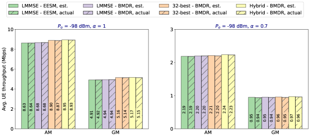
Figure 9: The AM and GM for the four detector schemes using PHY abstraction (compared with the actual values corresponding to Fig. 5) for (left) $\alpha=1$ and (right) $\alpha=0.7$.

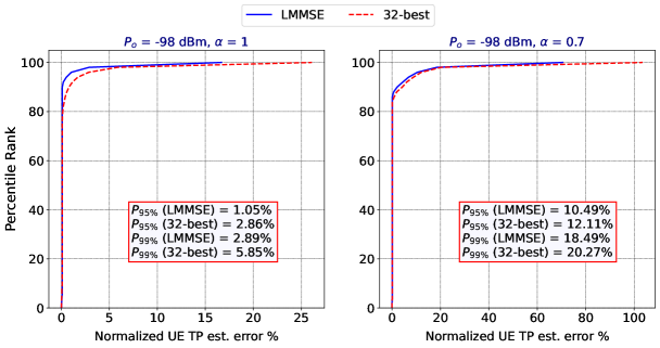
Figure 10: The percentiles of the normalized UE-throughput estimation error using PHY abstraction for the LMMSE detector and the $32$-best detector for (left) $\alpha=1$ and (right) $\alpha=0.7$.

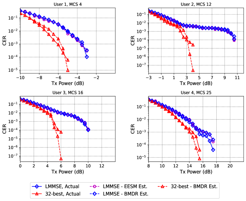
Figure 11: The link-level CER v. transmit power ($\mathrm{dB}$) plots for the LMMSE detector (both EESM and BMDR based) and the $32$-best detector for four UEs with different MCS levels. The solid lines correspond to the actual CERs and the dashed lines to the CERs estimated using the proposed abstraction technique.

We consider the same simulation setup as described in the previous subsection, but do not perform data transmission, LLR-generation, or channel decoding. We follow the method outlined in the flowchart of Fig. 3 and compute the AM and GM throughputs using the BMDR-CER mapping. To be precise, the MCS levels are selected as in the previous subsection, and the estimated SE is multiplied by the mapped CER for each notional codeword transmission. This is then averaged for all users in all the drops. The computed AM and GM throughputs are plotted in Fig. 9 alongside the actual values for all the four schemes. The efficacy of the EESM metric is well-known in the literature for linear detectors. Fig. 9 indicates that the BMDR-based PHY abstraction is equally effective for both linear and non-linear detectors.

The percentiles of the normalized UE-throughput estimation error are shown in Fig. 10 for the LMMSE and the $32$-best detectors with BMDR-based estimation. We haven’t included LMMSE-EESM in these plots because the corresponding plots are indistinguishable from that of LMMSE-BMDR. This normalized UE-throughput estimation error is calculated as follows: if the actual UE throughput is $TP_{actual}$ and the estimated throughput is $TP_{est}$, the normalized throughput estimation error is $|TP_{actual}-TP_{est}|/TP_{actual}$. Also marked in Fig. 10 are the $95^{th}$ and $99^{th}$ percentiles of the normalized estimation errors for both LMMSE and $32$-best detector. For example, in the case of $\alpha=0.7$, $P_{99\%}$ for the LMMSE detector with BMDR-based throughput estimation is $18.49\%$, which means that $95\%$ of the normalized UE-throughput estimation errors across all the drops are within $18.49\%$ of the true values, i.e., $|TP_{actual}-TP_{est}|/TP_{actual}\leq 0.1849$ for $95\%$ of the UEs. The results are much better for $\alpha=1$. The high deviations for the case of $\alpha=0.7$ are for UEs with very low throughput (possibly cell-edge UEs). In both the plots, the estimation errors are very low for a majority of the UEs for both the detectors.

In Fig. 11, we present the CER plots as a function of UE transmit power in a link-level simulation setting, with the channels generated using the QuaDRiGa channel-simulator [25]. In this plot, we have plotted the actual observed CER values (solid lines) along with the estimated CER (dashed lines) for the case of both EESM and BMDR. We consider four users with different MCS levels which correspond to the $64$-QAM MCS table in 5G NR [26, Table 5.1.3.1–1]. The number of transmitted codewords is limited to $10,000$ and hence, the estimated CERs deviate a little at values below $10^{-5}$. The curves for LMMSE-EESM and LMMSE-BMDR are nearly indistinguishable. The plots show that the proposed link-level modeling technique is quite useful in capturing the main behavior of the PHY components for both linear and non-linear detectors.

While it might be surprising to note that the $32$-best detector performs significantly better than the LMMSE detector in Fig. 11 while the same is not reflected in Fig. 5, the explanation is the following. The link-level plots were obtained using the QuaDRiGa channel-simulator for a single user drop, and the channels of the four users were highly correlated which implies that the channel matrices had large condition numbers. The condition number of a matrix is defined as the ratio of the largest singular value to the smallest singular value. When the condition number of a matrix, expressed in logarithmic form, exceeds $10\text{\,}\mathrm{dB}$, it is well-known that linear detectors perform significantly worse than the sphere-decoding variants [17]. The condition numbers of the channels generated by the QuaDRiGa channel-simulator exceeded $10\text{\,}\mathrm{dB}$ approximately $40\%$ of the time. On the other hand, the plots in Fig. 5 were obtained by co-scheduling users with low-channel correlation (as explained in Section VI-A) for which the LMMSE detector performs reasonably well. In the latter scenario, the $32$-best detector can only provide a marginal improvement over the LMMSE detector. The other important point to note is that since the number of surviving candidates is restricted to only $32$, the quality of the LLRs generated by the $32$-best detector is worse than that of the LMMSE detector at low transmit power levels. This effect is more visible in the case of $\alpha=0.7$ (Figs. 7–8). In order to see significantly enhanced throughputs for such a case, one might need to use a higher value of $K$ for the $K$-best detector ($K\geq 64$).

Remark 1.

The whole purpose of link-level modeling is to save time while performing SLS. PHY abstraction for linear detectors using BMDR has a time-complexity similar to that of existing techniques based on EESM, MIESM, CESM, or LESM. The proposed technique computes the post-equalization SINR and maps it to BMDR which is then mapped to a CER/BLER value. In the case of existing techniques, the post-equalization SINR is mapped to an effective SINR using the relevant ESM metric and a look-up table, and this effective SINR is then mapped to a CER/BLER value.

For the case of non-linear detectors, there is no existing technique for comparison. The natural question to ask is whether the complexity of the proposed BMDR prediction method in [1] is significantly lower than that incurred by actually performing the entire link-level simulation without abstraction. For non-linear receivers like the sphere-decoding variants, the complexity of generating LLRs for the system considered in Section II is exponential in $N$, where $N$ is the total number of transmitting streams from all the UEs. For any other iterative non-linear receiver like SIC, the very sequential nature of the algorithm induces time latency. The proposed BMDR prediction is machine-learning-based and needs the convolutional neural networks (CNNs) to be trained offline once. Each CNN for a MU-MIMO configuration has around $5000$ trainable parameters and any real-time usage entails low time-latency because there are no iterations.

VII Discussion and Concluding Remarks

In the second part of this two-part paper, we proposed a new algorithm for uplink link-adaptation in MU-MIMO systems that use arbitrary receivers. This algorithm uses BMDR as a metric for MCS selection in MU-MIMO systems, and it was shown to perform as well as the state-of-the art for LA with the LMMSE detector. More importantly, it was shown to be quite effective for LA with the $K$-best detector which is a popular non-linear detector in the literature for which there is no previously known technique to perform full-scale LA. We also proposed a hybrid strategy that dynamically selects the most suitable detector from a list of available detectors for improved performance. We next proposed a technique to perform PHY abstraction in MU-MIMO systems for arbitrary receivers. The proposed technique allows a simpler evaluation of complex non-linear receiver algorithms without significantly compromising on the accuracy of the performance metrics.

We remarked that Algorithm 2 is optimal for linear detectors and is possibly optimal for the $K$-best detector. Obtaining a low-complexity algorithm that can be proven to be optimal for a general class of non-linear detectors needs further investigation. In addition, the trade-off between computational complexity and spectral efficiency of a hybrid detector obtained by solving (12) for a variety of different weights can be another interesting future research direction. Further, one might even consider exploring the usage of BMDR in other applications such as user-pairing and MU-MIMO scheduling, where the task is to decide which among several users can be co-scheduled together such that the throughput and latency targets for each user are satisfactorily met when a particular non-linear detector is used.

The most computation-intensive task in both LA and PHY abstraction for non-linear detectors is the offline training of the BMDR-predictor. However, this is a one-time process and the need for retraining is minimal, making the proposed technique viable for practical purposes. Non-linear detectors are playing an increasingly important role in advanced wireless technologies, especially with the advent of machine-learning-based receivers. As the uplink traffic is expected to increase significantly in the future, we expect the concepts developed in this paper to be very useful in the next-generation wireless technologies.

References

- [1] K. P. Srinath and J. Hoydis, “Bit-Metric Decoding Rate in Multi-User MIMO Systems: Theory,” 2022, under review. [Online]. Available: https://arxiv.org/abs/2203.06271
- [2] P. Bertrand, J. Jiang, and A. Ekpenyong, “Link Adaptation Control in LTE Uplink,” in 2012 IEEE Vehicular Technology Conference (VTC Fall), 2012, pp. 1–5.
- [3] M. G. Sarret, D. Catania, F. Frederiksen, A. F. Cattoni, G. Berardinelli, and P. Mogensen, “Dynamic Outer Loop Link Adaptation for the 5G Centimeter-Wave Concept,” in Proceedings of European Wireless 2015; 21th European Wireless Conference, 2015, pp. 1–6.
- [4] S. Sun, S. Moon, and J.-K. Fwu, “Practical Link Adaptation Algorithm With Power Density Offsets for 5G Uplink Channels,” IEEE Wireless Communications Letters, vol. 9, no. 6, pp. 851–855, 2020.
- [5] W. Fu and J. S. Thompson, “Performance analysis of K-best detection with adaptive modulation,” in 2015 International Symposium on Wireless Communication Systems (ISWCS), 2015, pp. 306–310.
- [6] M. Shin, D. S. Kwon, and C. Lee, “Performance Analysis of Maximum Likelihood Detection for MIMO Systems,” in 2006 IEEE 63rd Vehicular Technology Conference, vol. 5, 2006, pp. 2154–2158.
- [7] Z. Guo and P. Nilsson, “Algorithm and Implementation of the K-best Sphere decoding for MIMO Detection,” IEEE J. Sel. Areas Commun., vol. 24, no. 3, pp. 491–503, 2006.
- [8] D. Tse and P. Viswanath, Fundamentals of Wireless Communication. USA: Cambridge University Press, 2005.
- [9] E. Viterbo and J. Boutros, “A Universal Lattice Code Decoder for Fading Channels,” IEEE Trans. Inf. Theory, vol. 45, no. 5, pp. 1639–1642, 1999.
- [10] C. Studer and H. Bölcskei, “Soft–Input Soft–Output Single Tree-Search Sphere Decoding,” IEEE Trans. Inf. Theory, vol. 56, no. 10, pp. 4827–4842, 2010.
- [11] L. G. Barbero and J. S. Thompson, “Fixing the Complexity of the Sphere Decoder for MIMO Detection,” IEEE Trans. Wireless Commun., vol. 7, no. 6, pp. 2131–2142, 2008.
- [12] 3GPP, “NR; Multiplexing and channel coding,” 3rd Generation Partnership Project (3GPP), Technical Specification (TS) 38.212, 12 2020, version 16.4.0. [Online]. Available: https://portal.3gpp.org/desktopmodules/Specifications/SpecificationDetails.aspx?specificationId=3214
- [13] K. Brueninghaus, D. Astely, T. Salzer, S. Visuri, A. Alexiou, S. Karger, and G.-A. Seraji, “Link performance models for system level simulations of broadband radio access systems,” in 2005 IEEE 16th International Symposium on Personal, Indoor and Mobile Radio Communications, vol. 4, 2005, pp. 2306–2311 Vol. 4.
- [14] L. Wan, S. Tsai, and M. Almgren, “A fading-insensitive performance metric for a unified link quality model,” in IEEE Wireless Communications and Networking Conference, 2006. WCNC 2006., vol. 4, 2006, pp. 2110–2114.
- [15] S. Lagen, K. Wanuga, H. Elkotby, S. Goyal, N. Patriciello, and L. Giupponi, “New radio physical layer abstraction for system-level simulations of 5G networks,” in ICC 2020 - 2020 IEEE International Conference on Communications (ICC), 2020, pp. 1–7.
- [16] G. Caire, G. Taricco, and E. Biglieri, “Bit-Interleaved Coded Modulation,” IEEE Trans. Inf. Theory, vol. 44, no. 3, pp. 927–946, May 1998.
- [17] J. Ketonen, M. Juntti, and J. R. Cavallaro, “Receiver implementation for MIMO-OFDM with AMC and precoding,” in 2009 Conference Record of the Forty-Third Asilomar Conference on Signals, Systems and Computers, 2009, pp. 1268–1272.
- [18] I.-W. Lai, G. Ascheid, H. Meyr, and T.-D. Chiueh, “Low-Complexity Channel-Adaptive MIMO Detection with Just-Acceptable Error Rate,” in VTC Spring 2009 - IEEE 69th Vehicular Technology Conference, 2009, pp. 1–5.
- [19] M. Cirkic, D. Persson, and E. G. Larson, “Allocation of Computational Resources for Soft MIMO Detection,” IEEE J. Sel. Topics in Signal Process., vol. 5, no. 8, pp. 1451–1461, 2011.
- [20] S. Chaudhari, H. Kwon, and K. Song, “Reliable and Low-Complexity MIMO Detector Selection using Neural Network,” in Int. Conf. Comput., Netw. and Commun. (ICNC) 2020, 2020, pp. 608–613.
- [21] H. Kwon and K. Song, “MIMO-OFDM Detector Selection using Reinforcement Learning,” in Int. Conf. Comput., Netw. and Commun. (ICNC) 2020, 2020, pp. 347–352.
- [22] 3GPP, “Study on channel model for frequencies from 0.5 to 100 GHz,” 3rd Generation Partnership Project (3GPP), Technical Specification (TS) 38.901, 12 2019, version 16.1.0. [Online]. Available: https://portal.3gpp.org/desktopmodules/Specifications/SpecificationDetails.aspx?specificationId=3173
- [23] ——, “NR; Physical layer procedures for control,” 3rd Generation Partnership Project (3GPP), Technical Specification (TS) 38.213, 12 2021, version 17.0.0. [Online]. Available: https://portal.3gpp.org/desktopmodules/Specifications/SpecificationDetails.aspx?specificationId=3215
- [24] S. Lagen, K. Wanuga, H. Elkotby, S. Goyal, N. Patriciello, and L. Giupponi, “New Radio Physical Layer Abstraction for System-Level Simulations of 5G Networks,” in IEEE Int. Conf. Commun. (ICC) 2020, 2020, pp. 1–7.
- [25] S. Jaeckel, L. Raschkowski, K. Börner, and L. Thiele, “QuaDRiGa: A 3-D Multi-Cell Channel Model With Time Evolution for Enabling Virtual Field Trials,” IEEE Trans. Antennas and Propag., vol. 62, no. 6, pp. 3242–3256, 2014.
- [26] 3GPP, “NR; Physical layer procedures for data,” 3rd Generation Partnership Project (3GPP), Technical Specification (TS) 38.214, 12 2020, version 16.4.0. [Online]. Available: https://portal.3gpp.org/desktopmodules/Specifications/SpecificationDetails.aspx?specificationId=3216