Spectroscopic Analysis Tool for intEgraL fieLd unIt daTacubEs (satellite): Case studies of NGC 7009 and NGC 6778 with MUSE

Abstract

Integral field spectroscopy (IFS) provides a unique capability to spectroscopically study extended sources over a 2D field of view, but it also requires new techniques and tools. In this paper, we present an automatic code, Spectroscopic Analysis Tool for intEgraL fieLd unIt daTacubEs, satellite, designed to fully explore such capability in the characterization of extended objects, such as planetary nebulae, H ii regions, galaxies, etc. satellite carries out 1D and 2D spectroscopic analysis through a number of pseudo-slits that simulate slit spectrometry, as well as emission line imaging. The 1D analysis permits direct comparison of the integral field unit (IFU) data with previous studies based on long-slit spectroscopy, while the 2D analysis allows the exploration of physical properties in both spatial directions. Interstellar extinction, electron temperatures and densities, ionic abundances from collisionally excited lines, total elemental abundances and ionization correction factors are computed employing the pyneb package. A Monte Carlo approach is implemented in the code to compute the uncertainties for all the physical parameters. satellite provides a powerful tool to extract physical information from IFS observations in an automatic and user configurable way. The capabilities and performance of satellite are demonstrated by means of a comparison between the results obtained from the Multi Unit Spectroscopic Explorer (MUSE) data of the planetary nebula NGC 7009 with the results obtained from long-slit and IFU data available in the literature. The satellite characterization of NGC 6778 based on MUSE data is also presented.

1 Introduction

Recent advances in integral field spectroscopy (IFS) have promoted a huge growth in imaging spectroscopy, demanding new approaches to the study of extended and resolved objects. Over the last two decades several integral field units (IFU) have been built covering mainly optical and infrared wavelengths, with diverse characteristics, such as field of view, wavelength coverage, spatial resolution, resolving power (see conference review on IFS, Allington2006; Mediavilla2011).

IFS provides data in 3 dimensions (2 spatial and 1 spectral) or, equivalently, a cube of data where each wavelength element corresponds to a spectral image. These data cubes make possible the simultaneous spectroscopic analysis of extended objects (e.g. galaxies, H ii regions, planetary nebulae) in both spatial directions providing the spatial distribution of emission lines fluxes, line ratios and the nebular physical parameters (e.g. extinction, electron temperature and density ($T_{e}$, $N_{e}$), abundances), a task that is very time-consuming with traditional long-slit spectroscopy techniques (e.g. Monteiro2004; Monteiro2005; Phillips2010; Ferreira2011) or CCD imaging spectroscopy (e.g. Jacoby1987; Lame1994; Lame1996).

These advances have boosted the number of works devoted to spatially resolved studies of planetary nebulae (PNe) using IFS over the last decade; some representative examples of these studies are, e. g. Tsamis2008, Monteiro2013, Ali2016, Walsh2016, Walsh2018, Ali2019, Monreal2020, Akras2020a, and Garciarojas2022.

The vast majority of spectroscopic studies of extended objects have been performed employing the traditional long-slit spectroscopy. As a consequence, spectroscopic data are available only for specific regions where the slits or apertures were placed. Moreover, diagnostic diagrams such as BPT (Baldwin1981), VO (Veilleux1987) and STB (Sabbadin1977), built to distinguish AGN, LINERs, and Seyfert galaxies or PNe, SNRs and H ii regions are also based on 1D long-slit data as well as simulations from 1D models such as cloudy (Ferland2013; Ferland2017) and mappings (Sutherland2017; Sutherland2018).

From IFU data, besides the unique 2D spectroscopic analysis, it is also possible to perform 1D analysis by simulating slit apertures (hereafter “pseudo-slits”). This is essential to acquire results that can be properly compared with those from long-slit studies present in the literature. For instance, it has already been pointed out that a spaxel-by-spaxel analysis of emission line ratios of extended sources from IFUs is not recommended for a straightforward comparison with integrated long-slit spectra and the resultant diagnostic diagrams (Ercolano2012; Morisset2018; Akras2020a).

In this paper, we present a newly developed automatic code that performs a full spectroscopic analysis of extended sources using IFS data, namely “Spectroscopic Analysis Tool for intEgraL fieLd unIt daTacubEs (satellite)”. The novelty of this tool is that it provides an 1D spectroscopic analysis through pseudo-slits and 2D analysis through maps. The former will allow to properly compare the results obtained from IFUs with those from previous 1D long-slit spectroscopy while the latter will allow to explore the extended sources in both spatial directions. A brief presentation of the capabilities of satellite is presented in Akras2020a using VIMOS IFS data of the PN Abell 14.

The paper is organized as follows. In Section 2, we present the four modules of the satellite code available in the current version namely: (I) rotation analysis, (II) radial analysis, (III) specific slits analysis and (IV) 2D analysis. In Sections 3 and 4, we apply the satellite code to the Multi Unit Spectroscopic Explorer (MUSE) Science Verification data of the PN NGC 7009, as well as the data from program 097.D-0241(A) (PI: Corradi). A comparison between satellite’s results and those from Walsh2018 is presented as well as the outcomes from the two MUSE datacubes. In Section 5, we apply the satellite code to the MUSE data of NGC 6778 and perform the 1D and 2D spectroscopic characterization of the nebula. The results of this work as well as the potential upgrades to future versions of the satellite code are discussed in Section 6.

2 The satellite code

The Spectroscopic Analysis Tool for intEgraL fieLd unIt daTacubEs (satellite) is a newly developed python 3 code that performs a number of spectroscopic analyses on IFU data. As input, satellite uses the flux maps of several emission lines usually detected in galaxies, H ii regions and PNe, extracted from IFU datacubes.

satellite simulates pseudo-slit spectra by summing up the values of each individual spaxel (the unit of the IFU) within the specific region defined by the width and length of the pseudo-slits provided by the user. Note that the pseudo-slits are built considering full-size spaxels and no partially covered ones.

To exclude values from problematic spaxels or with low signal-to-noise (S/N) ratio, two criteria must be satisfied by each spaxel: (i) F(H $\alpha$)$>$0, F(H $\beta$)$>$0 and (ii) F(H $\alpha$)$>$2.85*F(H $\beta$), to avoid unrealistic values for the interstellar extinction coefficient (c(H $\beta$)).

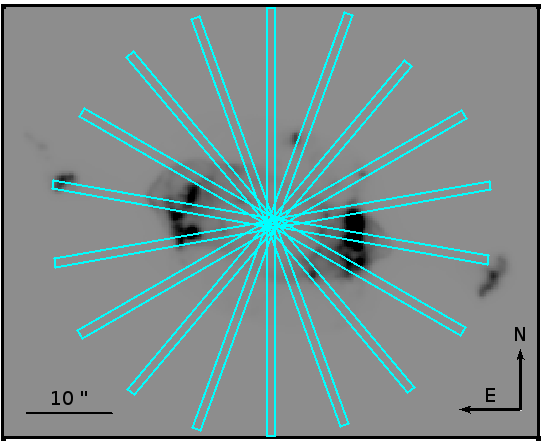
Figure 1: Illustrative example of pseudo-slits positions in NGC 7009 overlaid on the [N ii] 6584Å image for the rotation analysis module. The width, length, initial, final and step angle are provided by the user. The size of the image is 62$\times$50 arcsec.

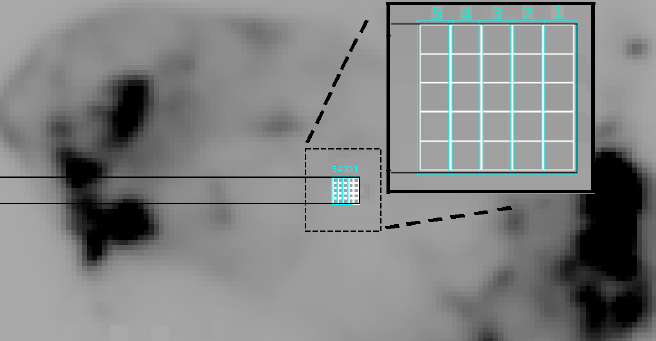
Figure 2: Illustrative example of the radial analysis module for the PA=90 degrees pseudo-slit in NGC 7009 overlaid on the [N ii] 6584Å image. The inset image shows a zoomed-in of the pseudo-slit. The boxes correspond to the spaxels of the IFU. The fluxes of the spaxels in each numbered column/row are summed up to get the total flux for each column/row within the width of the pseudo-slit or equivalently to the distance from the central star taking into account the pixel scale of the IFU.

For all the modules, satellite first calculates c(H $\beta$) considering an extinction curve law selected by the user among the options in the pyneb package version 1.1.15 (Luridiana2015). Then it computes the physical parameters of the ionized nebula such as $T_{e}$ and $N_{e}$, ionic abundances, ionization correction factors (ICFs), total elemental abundances and abundance ratios, employing the pyneb package. In this work, we used the default atomic databases in the pyneb package (see Morisset2020). The diagnostic lines for the determination of $T_{e}$ and $N_{e}$ as well as the values applied for the ionic abundances determinations are set by the user from a list of diagnostics. The uncertainties of the physical parameters are computed following Monte Carlo simulations. The number of random spectra (hereafter replicate spectra) is chosen by the user and they are generated considering a Gaussian distribution centred at a reference spectrum (i.e. line intensities) with a sigma equal to the uncertainty of each line intensity computed from the provided error maps. Then, all the physical parameters are computed for each replicate spectrum and the resultant standard deviation of the distribution of each parameter is considered to be the final uncertainty provided by the satellite code. Besides the calculations of nebular physical parameters for the pseudo-slits, satellite also provides scatter plots, emission line diagnostic diagrams, histograms and 2D maps for all nebular parameter. The modules of satellite are described below.

2.1 Rotation analysis module

This module deals with the spectroscopic analysis of an extended source from a number of pseudo-slits placed radially across half of the nebula with position angles (PAs) from 0 to 360 degrees (Fig. 1). satellite first rotates all raw images (line flux maps) and then generates new images from which it computes the fluxes summing up the values of each individual pixel with the pseudo-slit. The pseudo-slits are always in vertical direction (up-and-down orientation).

PA=0 degrees corresponds to a pseudo-slit in vertical orientation on the map and increases as the pseudo-slit rotates in the anti-clockwise direction. If the IFU data and the line flux maps are oriented such that North is up and East is left, the PA of the pseudo-slits in the satellite’s frame coincides with the slits’s PA on-sky values (PA=0 degrees in the North-South direction and increases rotating East from North). The initial, final and step angles of the position angle as well as the width and the length of the pseudo-slits are given by the user.

All the line intensities and physical parameters of the nebula are derived for each pseudo-slit. Therefore, this module provides an analysis of nebular gas (c(H $\beta$), $T_{e}$ and $N_{e}$, ionic and elemental abundances, ICFs) as functions of slit PA as well as an ASCII file (a multi-column list of data used for the plots) so that users can construct their own plots.

2.2 Radial analysis module

The radial analysis module computes the emission line fluxes along a specific pseudo-slit as a function of the distance from the geometric center and/or the ionizing source (e.g. central star). The characteristics of this pseudo-slit (PA, width and length) are free parameters provided by the user. satellite calculates the line fluxes summing up the values of the individual spaxels in one column/row enclosed by the pseudo-slit (Fig. 2) and then all the physical parameters of the nebula at each column/row). Scatter plots for each parameter as a function of the distance taking into account the pixel scale of the IFU are provided as well as an ascii file with the data. The distance from the central star at which each emission line shows a peak is also determined. The emission lines for this task are also chosen by the user. Overall, the radial analysis module makes possible the study of nebular parameters and line ratios as a function of the distance from the central ionising source of the nebula.

2.3 Specific slits analysis module

The specific slits analysis module performs a full spectroscopic analysis for 10 (default number in satellite v1.3) distinct regions that can be configured so as to study specific features/regions that possess distinctive morphological or physical properties, such as lobes, ansae, low-ionization structures (LISs), rim, etc. in PNe for a direct comparison with the results from long-slit studies.

Line intensities and physical parameters are calculated for each specific region defined by the pseudo-slits summing up all the spaxels values. The exact position/centre, PA, width and length of the pseudo-slits are not necessarily the same and are provided by the user. Fig. 3 displays the 10 selected regions for the analysis of NGC 7009 overlaid on its [N ii] 6584Å image.

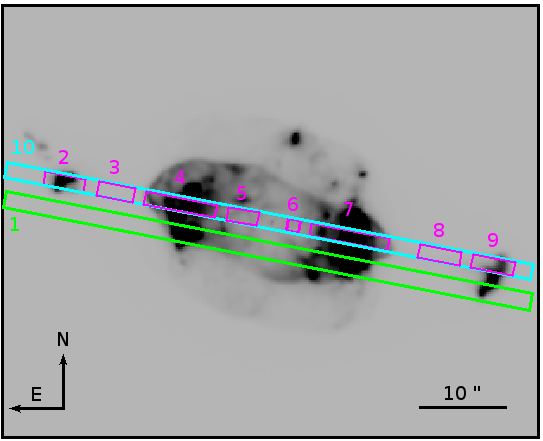
Figure 3: Ten selected regions in NGC 7009 overlaid on the [N ii] 6584Å image. The position of the centre (x, y coordinates), position angle, width and length of the slits are free parameters provided by the user. Slits 1 and 10 represent the slits position from Fang2011 and Goncalves2003, respectively. Numbered regions from 2 to 9 correspond to the sub-structures of knots and jet-like, or sub-regions of rims defined in Goncalves2003. The size of the image is 62$\times$50 arcsec.

Table 1: Comparison between satellite and Walsh2018 results obtained from the NGC 7009 Science Verification MUSE data. Flux maps used for this comparison were those extracted by Walsh2018.

Parameter	satellite	SD${}^{\dagger}$	Walsh2018	SD	Log(ratio)	SD	# of spaxels
c(H $\beta$)	0.105	0.065	0.122	0.041	-0.022	0.165	28070
Te(SIII6312_9069)_Ne(ClIII5517_5538)	9166	301	9159	326	0.0005	0.0024	17305
Ne(ClIII5517_5538)_Te(SIII6312_9069)	3609	2037	3547	2476	0.0001	0.0015	17305
log(He i  5876/H $\alpha$)	-1.264	0.035	-1.270	0.031	-0.004	0.002	35876
log(He ii  5412/H $\beta$)	-2.443	0.484	-2.425	0.484	0.004	0.001	14427
log([N II] 6583/H $\alpha$)	-1.465	0.379	-1.447	0.336	0.0001	0.0014	39302
log([O I] 6300/H $\alpha$)	-2.953	0.833	-2.880	0.863	-0.0009	0.0007	11720
log([O iii] 4959/H $\beta$)	0.666	0.080	0.699	0.078	-0.0025	0.0016	40724
He+ (5876)/H+	0.105	0.008	0.102${}^{{\dagger}{\dagger}}$	0.009	0.013	0.012	16516
He+ (6678)/H+	0.100	0.008	0.102${}^{{\dagger}{\dagger}}$	0.009	-0.010	0.010	16516
He^++ (5412)/H+	0.007	0.008	0.007	0.008	-0.001	0.003	14042
N+ (6548)/H+ (10${}^{-6}$)	5.688	14.499	5.875${}^{{\dagger}{\dagger}}$	14.66	-0.017	0.014	17304
N+ (6584)/H+ (10${}^{-6}$)	5.789	14.752	5.875${}^{{\dagger}{\dagger}}$	14.66	-0.009	0.014	17304
O+ (7320)/H+ (10${}^{-5}$)	3.491	3.384	3.068	2.703	0.060	0.031	17296
O+ (7330)/H+ (10${}^{-5}$)	3.728	3.351	3.068	2.703	0.090	0.028	17283
O^++ (4959)/H+ (10${}^{-4}$)	5.659	0.688	5.992	0.765	-0.024	0.011	17253
S+ (6716)/H+ (10${}^{-7}$)	3.176	6.882	2.977${}^{{\dagger}{\dagger}}$	6.101	0.014	0.055	17301
S+ (6731)/H+ (10${}^{-7}$)	2.927	6.102	2.977${}^{{\dagger}{\dagger}}$	6.101	-0.010	0.014	17305
S^++ (6312)/H+ (10${}^{-6}$)	4.490	1.548	4.616	1.618	-0.012	0.017	17305
Cl^++ (5517)/H+ (10${}^{-7}$)	0.998	0.240	1.019	0.248	-0.009	0.012	17305
Ar^++ (7136)/H+ (10${}^{-6}$)	1.645	0.337	1.837	0.384	-0.048	0.015	17305

${}^{{\dagger}}$ Standard Deviation from the whole map. ${}^{{\dagger}{\dagger}}$ These are average ionic abundances from both ions. (Walsh2018) data are available in the The Strasbourg astronomical Data Center (http://cdsarc.u-strasbg.fr/viz-bin/qcat?J/A+A/620/A169)

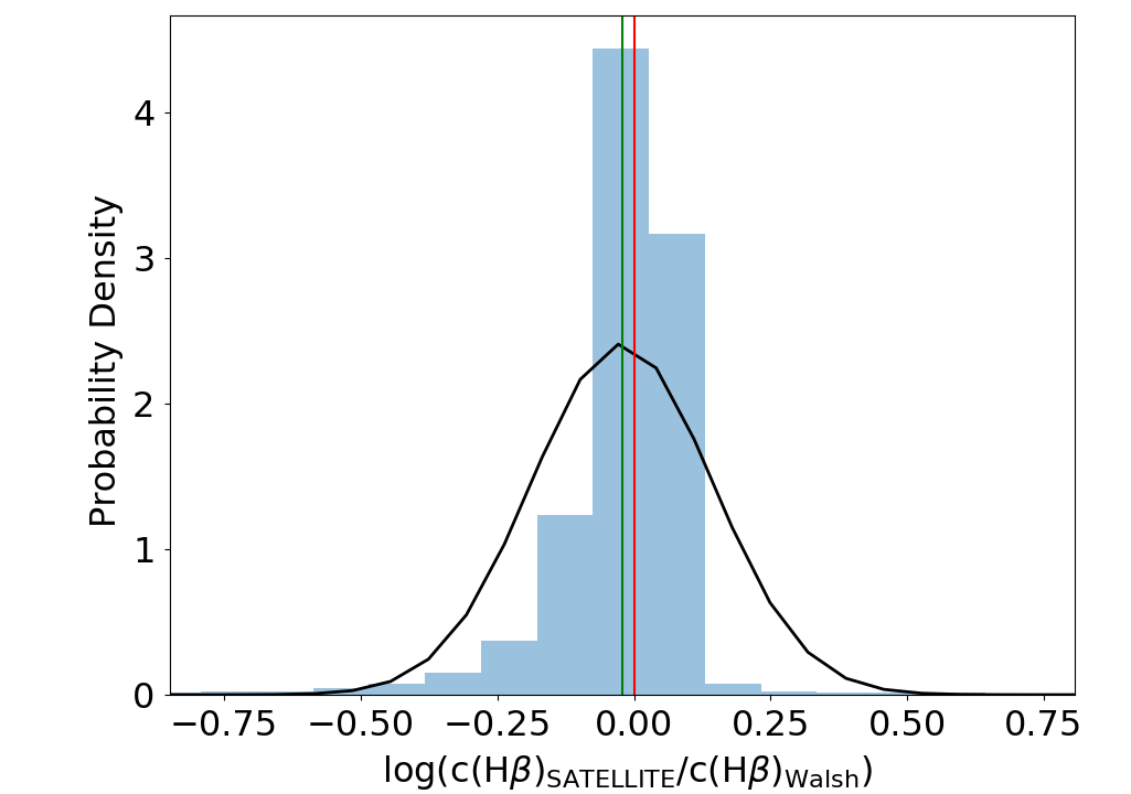
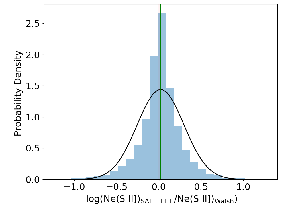
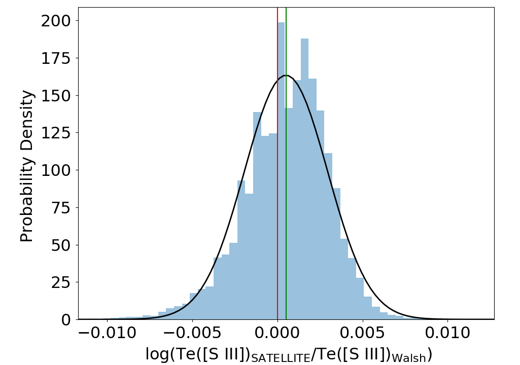
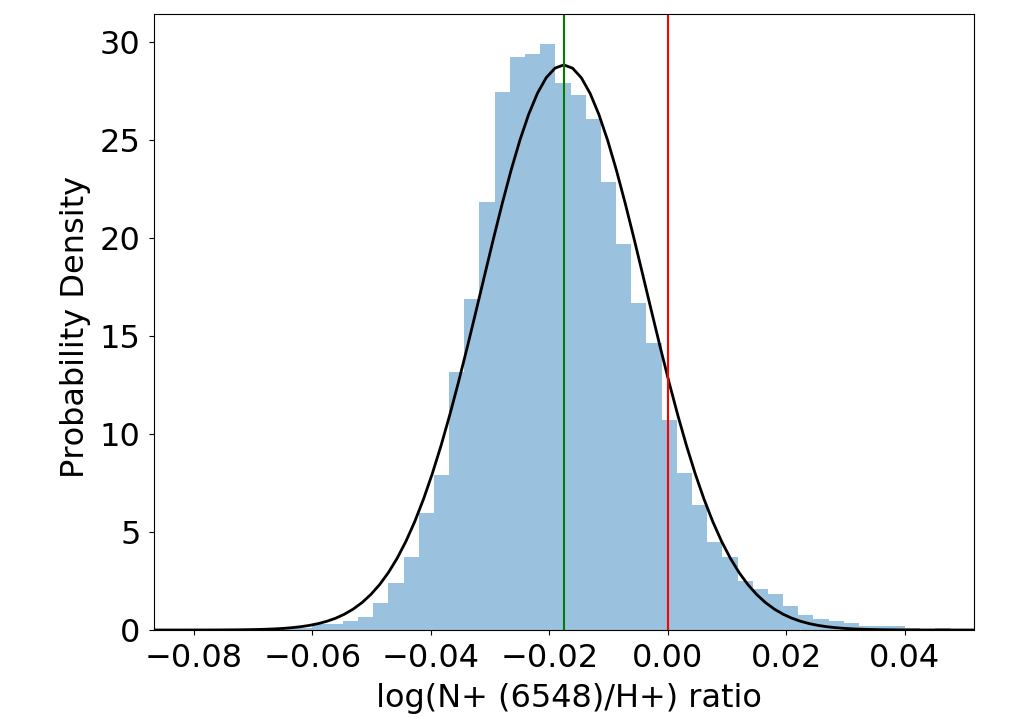
Figure 4: Comparison distributions of the log(c(H $\beta$)${}_{\rm{\sc satellite}}$ / c(H $\beta$)${}_{\rm{Walsh}}$) (upper, left panel), log($N_{e}$[S ii]${}_{\rm{\sc satellite}}$ / $N_{e}$[S ii]${}_{\rm{Walsh}}$) (upper right panel), log($T_{e}$[S iii]${}_{\rm{\sc satellite}}$ / $T_{e}$[S iii]${}_{\rm{Walsh}}$) (lower left panel) and log(N^+(6584)/H^+${}_{\rm{\sc satellite}}$ / N^+(6584)/H^+${}_{\rm{Walsh}}$) ratios (lower right panel) between the results obtained with satellite and computed by Walsh2018. Red and green vertical lines indicate the zero value and the peak of each distribution. The black lines represent the probability density functions of the data.

2.4 2D analysis module

The fourth satellite module performs the full 2D spectroscopic analysis. This module calculates the line intensities and physical parameters in each spaxel and only for those that satisfy the aforementioned criteria. The principal outputs of this module are 2D maps of line ratios, nebular parameters, ionic and total elemental abundances as well as the corresponding histograms of their distributions. Moreover, the mean values, standard deviations and percentiles of 5%, 25% (Q1), 50% (median), 75% (Q3), 95% are also calculated for all the line ratios and nebular parameters.

A number of emission line diagnostic diagrams (including the classical BPT/VO, STB) selected by the user among a pre-defined list in satellite are also generated and provided. There is an option to plot the values obtained from the rotation analysis and specific slits analysis modules and the 2D analysis from all spaxels on the same diagnostic diagrams.

The comparison of the emission line ratios from individual spaxel line ratios with the ratios obtained from integrated slits is crucial for the study of extended sources such as galaxies, H ii regions and PNe and the interpretation of the excitation mechanisms (Ercolano2012; Morisset2018; Akras2020a). Moreover, the available Ionization Correction Factors (ICFs) formulae for the computation of the total elemental abundances can be made only for 1D spectra rather than for each individual spaxel. The ionization structure of PNe is strongly dependent on the distance from the UV-source (e.g. PN central star) which can lead to misleading 2D abundances estimations.

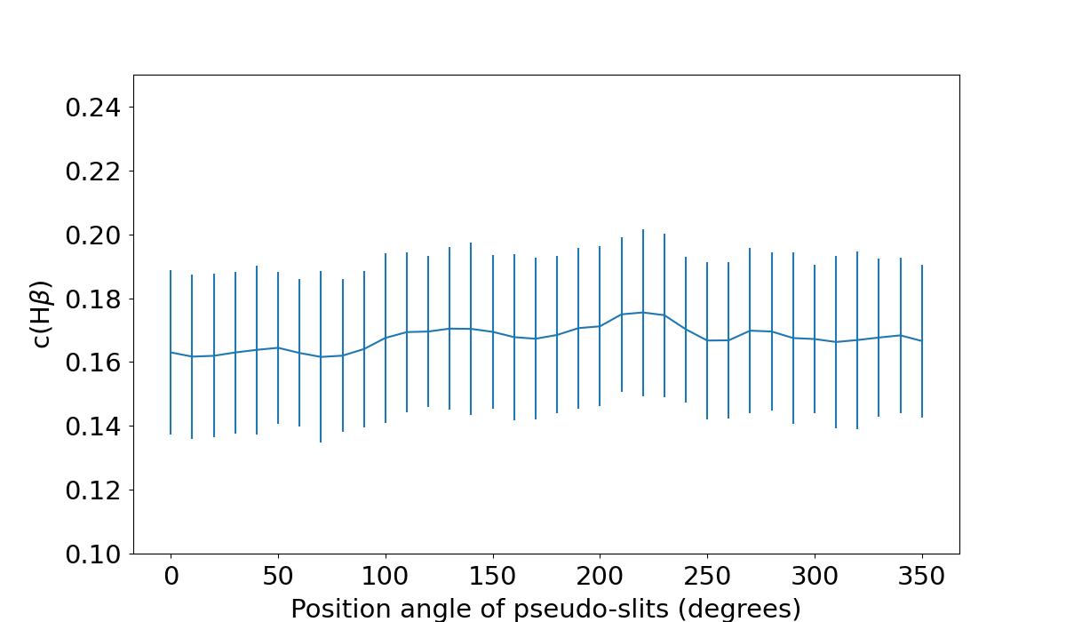
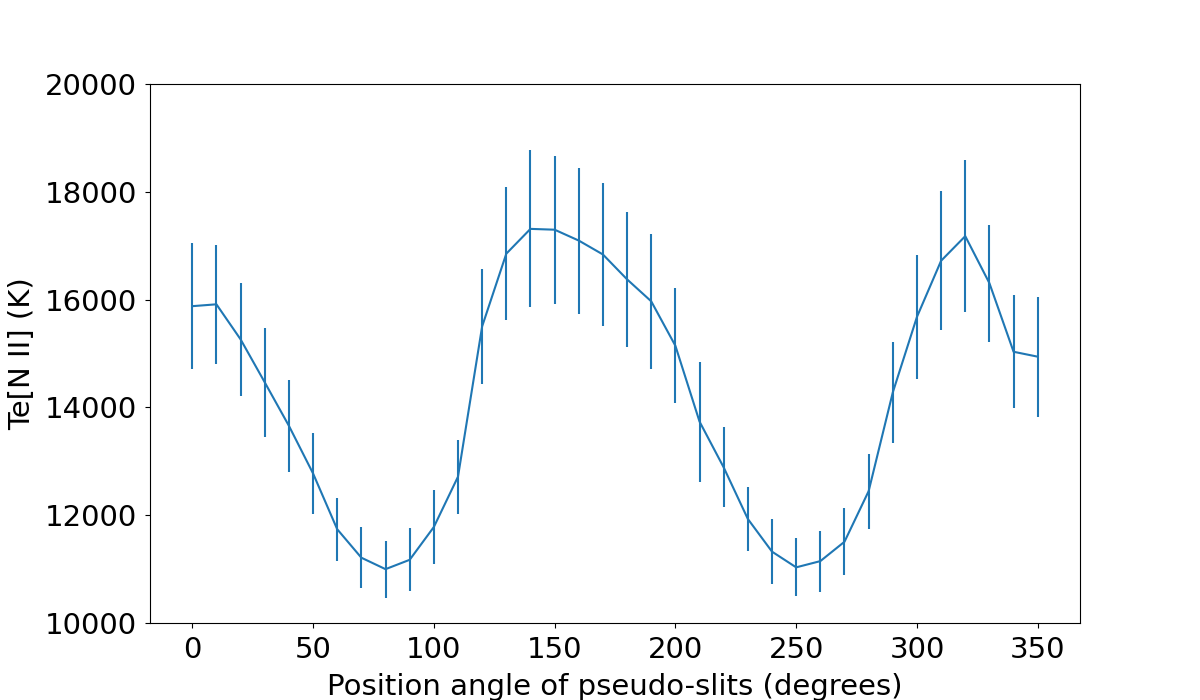
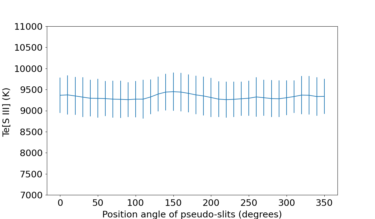
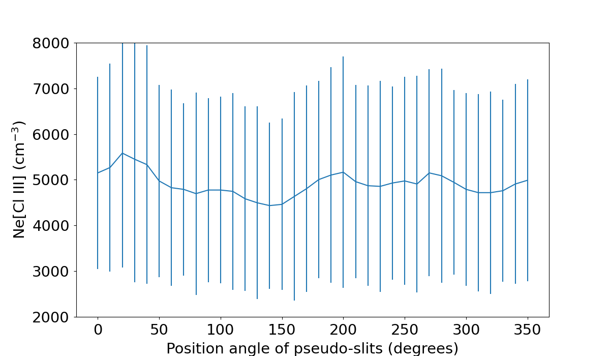
Figure 5: c(H $\beta$) (first panel), $T_{e}$[N ii](second panel), $T_{e}$[S iii](third panel), and $N_{e}$[Cl iii](fourth panel) versus the position angle of the pseudo-sits. PA=0 degrees corresponds to a pseudo-slit oriented north-south and increases rotating to the east.

3 Case study of NGC 7009 with the Science Verification MUSE data

In order to illustrate further and assess the numerical tools provided by satellite, we use as a case study the planetary nebula NGC 7009, also known as the Saturn nebula, and it is among the most extensively studied PNe. Observations covering a large portion of the electromagnetic spectrum are available. Its high surface brightness has made possible various thorough studies using both imaging and spectroscopic data (e.g. Lame1996; Guerrero2002; Rubin2002; Goncalves2003; Sabbadin2004; Goncalves2006; Rodriquez2007; Steffen2009; Phillips2010; Fang2011; Fang2013; Akras2020b). As a consequence, NGC 7009 was also an ideal object for MUSE (Bacon2010) Science Verification (SV) phase, and the first results from these data have been published by Walsh2016; Walsh2018.

The same emission line flux maps extracted from the SV MUSE datacube (Walsh2018) available in VizieR On-line Data Catalog(J/ApJ/889/49) are used to test the performance of the satellite code and compare its outputs with those from Walsh2018 as well as the long-slit spectra from Fang2011 and Goncalves2003. The resulting maps from satellite and Walsh2018 are first compared through a spaxel-by-spaxel approach. For this exercise, the same Galactic extinction law from Seaton1979 was considered for the spectroscopic analysis with satellite. Table 1 lists the mean values and standard deviations for the maps of some physical parameters, logarithmic line ratios and ionic abundances. For the majority of the parameters the difference is found to be less than 5 percent with comparable dispersion (similar standard deviations). Note that the current version of the satellite code does not correct for the contribution of recombination lines which may not be negligible, especially in PNe with relatively large abundance discrepancy factors between optical recombination lines and collisionaly excited lines, where this correction can be extremely problematic (see GomezLlanos2020). This explains the difference in the abundance of singly ionized Oxygen between satellite and (Walsh2018) as the O^++ recombination contribution results in 30 percent higher O^+/H+. The $T_{e}$[S iii] and $N_{e}$[Cl iii] diagnostic line were considered for all the calculations in order to replicate the exact outputs from Walsh2018.

Fig. 4 displays some representative examples of comparison histograms of different parameters and abundance ratios obtained from the satellite code and Walsh2018. Probability density functions are also shown (black line) with peaks very close to zero, which verifies the consistency and robustness of the code.

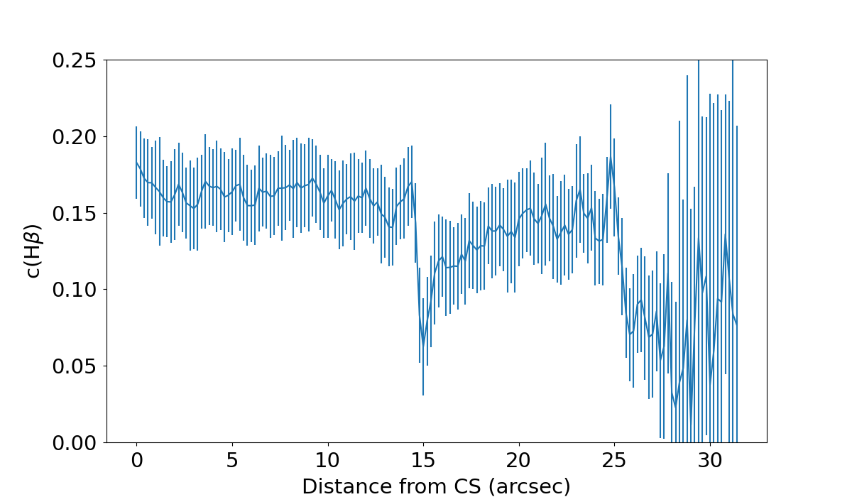
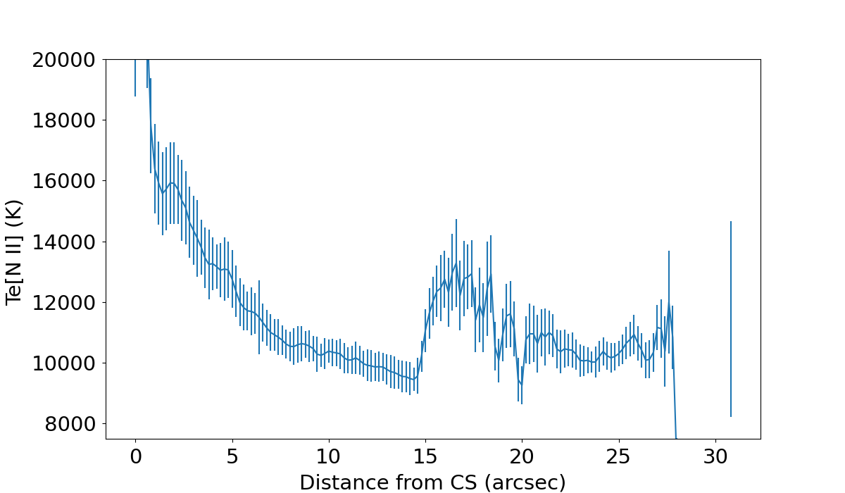
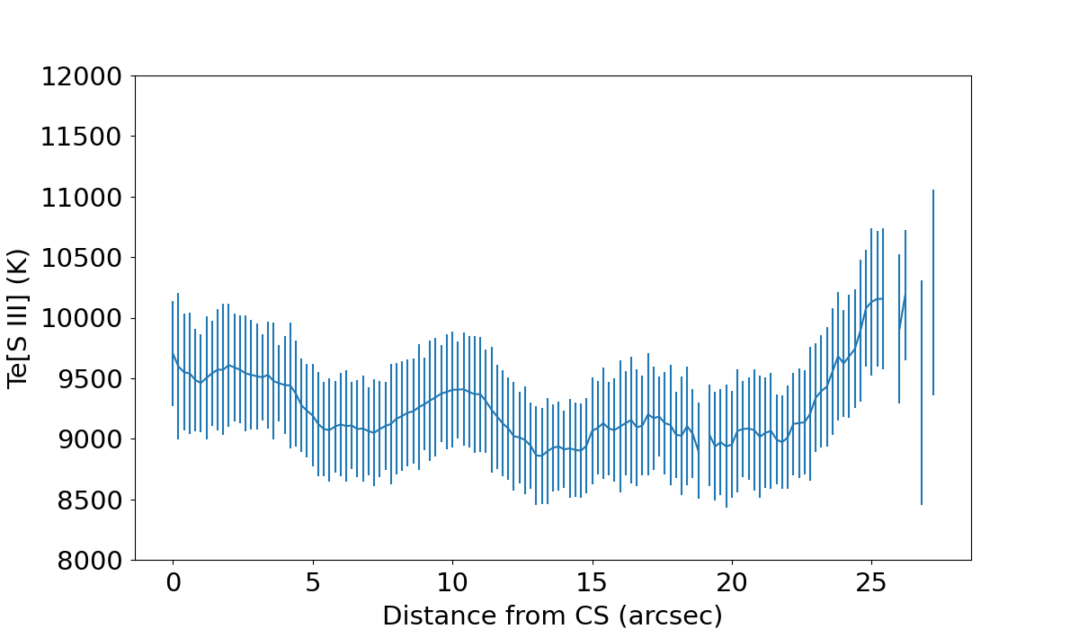
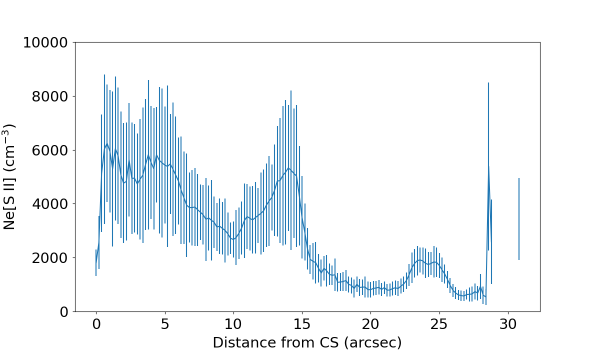
Figure 6: c(H $\beta$) (first panel), $T_{e}$[N ii] (second panel), $T_{e}$[S iii] (third panel) and $N_{e}$[S ii] (fourth panel) as a function of the distance from the central star (in arcsec) in a pseudo-slit at PA=79 degrees.

3.1 Rotation analysis module

The complex morphology of NGC 7009 composed of the ellipsoidal main nebula, several sets of outer shells, loops, jet-like features and pairs of LISs, make it an ideal nebula for demonstrative purposes of satellite’s capabilities and the rotation analysis module. The position angle of the pseudo-slits varies from 0 to 360 with a step of 10 degrees. Fig. 5 illustrates the variation of c(H $\beta$) (first panel), $T_{e}$[N ii] (second panel), $T_{e}$[S iii] (third panel) and $N_{e}$[Cl iii] (forth panel) as functions of the PA.

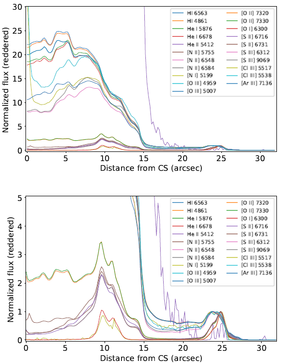
Figure 7: Radial distribution of emission lines normalized to 1. The normalization is made at the peak values for distances $>$20 arcsec. Lower panel zooms in to better illustrate the distribution of weaker lines.

c(H $\beta$) slightly varies with the PA from 0.16 to 0.17 but it can be considered constant within the uncertainties. Thus, no divergence along the direction of the jet-like/LISs is found. $T_{e}$[N ii] shows strong variation with the PA between 10000 K up to 17000 K. However, this variation shall not be considered real. It is associated with the high values in the central region of the nebula reported by Walsh2018. On the other hand, $T_{e}$[S iii] displays a constant value of $\sim$9400 K, being 2000 K lower than the values estimated by Fang2011 despite the good agreement in line intensities. It should be noted that Fang2011 measured $T_{e}$ from the $T_{e}$[S iii] 6312/(9069+9530) line ratio while satellite considers the $T_{e}$[S iii] 6312/9069 ratio. From the reported intensities of the nebular [S iii] lines by Fang2011, [S iii] $\lambda$9530 line is likely dimmed by atmospheric absorption bands (the [S iii] $\lambda$9531/$\lambda$9069 ratio is 1.88 in contrast with the expected theoretical value of 2.48 from the transition probabilities of Mendoza1982) resulting in higher temperature. This disagreement in $T_{e}$[S iii]  is also responsible for the difference in the ionic abundances showed in Table 1. Nevertheless, the results from the Cor MUSE data ((097.D-0241(A), PI: R. L. M. Corradi; see Section 4) agree with the results from the earlier MUSE SV data. $N_{e}$[Cl iii]  can also be considered constant within the uncertainties. To avoid possible false variations in the chemical abundances of the nebula, $T_{e}$[S iii] and $N_{e}$[Cl iii] were used to derive the chemical abundances and replicate the results from Walsh2018.

Table 2: Distances of the outer emission line peak from the central star in a pseudo-slit at PA=79 degrees.

Line	Distance${}^{{\dagger}}$	Line	Distance
	(arcsec)		(arcsec)
H i 4861Å	23.6	[N ii] 6584 Å	24.8
[O iii] 4959 Å	23.8	H i 6563Å	23.6
[N i] 5199 Å	24.8	[N ii] 6548 Å‘	24.8
He ii 5412Å	20.2	He i 6678Å	23.8
[Cl iii] 5517 Å	24.2	[S ii] 6717 Å	24.8
[Cl iii] 5538 Å	24.4	[S ii] 6731 Å	24.8
[N ii] 5755 Å	24.2	[Ar iii] 7136 Å	24.8
He i 5876Å	23.6	[O ii] 7320 Å	24.8
[O i] 6300 Å	24.8	[O ii] 7330 Å	24.8
[S iii] 6312 Å	23.8	[S iii] 9069 Å	23.8

${}^{{\dagger}}$ The spacial resolution of MUSE maps is 0.2 arcsec.

3.2 Radial analysis module

In Fig. 6, we present the variation of c(H $\beta$) (first panel), $T_{e}$[N ii] (second panel), $T_{e}$[S iii] (third panel) and $N_{e}$[S ii] (fourth panel) as functions of the distance from the central star for a slit at PA=79 degrees (along the direction of the eastern jet/knot). c(H $\beta$) is nearly flat ($\sim$0.16) for a distance up to 14-15 arcsec from the central star where it drops sharply to 0.06. This position corresponds exactly to the end of the ellipsoidal structure and the beginning of the jet-like structure. This drop in c(H$\beta$) is also highlighted in Walsh2016. Then it gradually increases from 0.06 up to 0.16 at the distance of 25 arcsec. Above that distance, the diffuse and weaker H $\alpha$ and H $\beta$ emission lines from the halo lead to large uncertainties and no robust results can be extracted.

[N ii] diagnostic lines yield a very high electron temperature in the inner nebula ($<$8 arcsec), which corresponds the the high value reported by Walsh2018, and at a distance of 15-17 arcsec from the central star, where there is a peak of $\sim$14000 K. It is worth noting the radial distribution of $T_{e}$[S iii]. For distances up to $\sim$22 arcsec, $T_{e}$[S iii] is nearly constant ($\sim$9200 K) and then it slightly increases to $\sim$10500K. This increase of $T_{e}$[S iii]  may be associated with a change of ionization and physical conditions across the LIS, shock heating process or photoelectric heating by dust. Intriguingly, the model of the nebula from Sabbadin2004 shows an increasing $T_{e}$[S iii]  with the distance from the central star ending with a bump at the position of the LISs (see their fig. 10). As for $N_{e}$, both diagnostics ([S ii] and [Cl iii]) display a very similar radial distribution with clear bumps at 11$<$r$<$15 arcsec and 23$<$r$<$26 arcsec the exact positions of K2/K4 and K1/K4 sub-structures, respectively (see Goncalves2003).

Besides the radial distribution of the line fluxes as a function of the distance from the central star, the radial analysis module also provides the distance from the central star in which each line peaks for a specific region in the nebula defined by the user. For the case of NGC 7009 (Fig. 7), the radial distributions of emission lines are normalized to unity for distances $>$20 arcsec (focused at the NE-LISs). The moderate/high ionization lines (e.g. [O iii], [Ar iii]) as well as the recombination lines H $\alpha$ and H $\beta$ are brighter in the inner nebula and drops outwards from 10 arcsec from the central star and peak again at the position of the knots (r=23-26 arcsec). On the other hand, the low ionization lines show a first peak at the position of the K2(K3) sub-structures around 10 arcsec and a second one at the position of the K1(K4) knots (Goncalves2003).

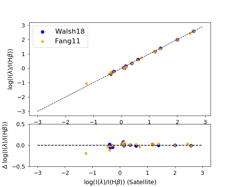
Figure 8: Comparison of the line ratios relative to H$\beta$=100 for the pseudo-slit at PA=79 degrees along the major axis of NGC 7009 studied by Fang2011. The line ratios from Fang2011 (labelled as Fang 11) and those reported by (Walsh2018, labelled as Walsh 18) are compared to the line ratios from the MUSE data using SATELLITE.

Note that the moderate/high and low-ionization lines peak at difference radial distances from the central star (see lower panel of Fig. 7). In Table 2, we list the distance from the central star where each line shows an augmentation at the position of $\sim$ 25 arcsec (K1 knot, Goncalves2003) and a clear stratification is found. In particular, the low-ionization lines (e.g., [N ii], [O ii], [S ii], etc.) peak at a distance of 24.8 arcsec, while the moderate/high ionization lines (e.g., [O iii], [S iii], [Cl iii], etc.) display a peak closer to the central star by 0.6-1 arcsec (Fig. 7).

3.3 Specific slits analysis module

For a direct comparison of the pseudo-slits spectra with previous long-slit spectroscopic data of NGC 7009 (Goncalves2003; Fang2011), we employed the specific slits module to replicate the observations. Line intensities are computed by satellite for a number of slit positions/regions (Fig. 3, Table 3). Fig. 8 displays the comparison between the line intensities computed from satellite and those from Walsh2018 and Fang2011 for the slit 1. For the interstellar extinction, we consider the same laws used in the studies above i.e., Howarth1983 for the pseudo-slit 1 and Cardelli1989 for the rest of the pseudo-slits. It should also be noted that for the estimation of the ionic and total abundances in this module, $T_{e}$[N ii]  and $N_{e}$[S ii] were considered for the low-ionization species while $T_{e}$[S iii]  and $N_{e}$[Cl iii]  were used for the moderate/high ionization species.

A reasonable agreement within the uncertainties is found for most of the line intensities as well as for the physical parameters c(H $\beta$), $T_{e}$, $N_{e}$ and abundances (Table 3). The uncertainties of the physical parameters are calculated considering a Monte Carlo approach and vary from 10 to 30 percent. Higher uncertainties are found for the sub-structures (K or J) because of the small size of the extracted windows (i.e. number of spaxels).

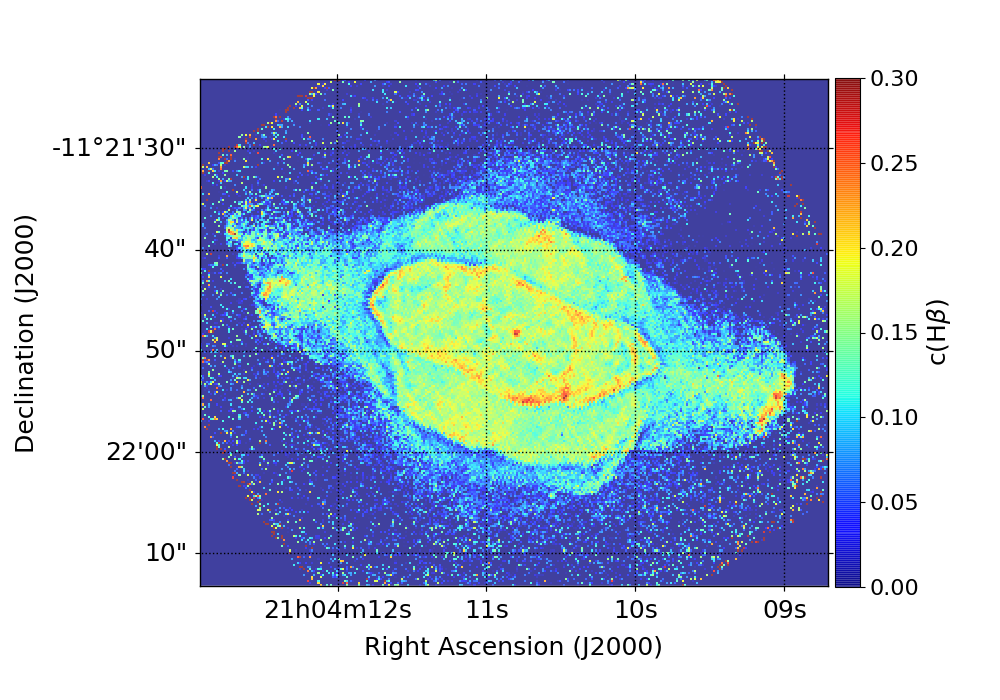
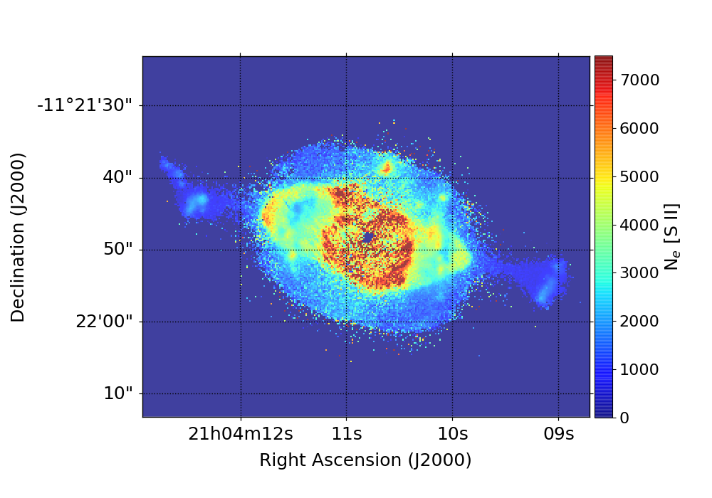
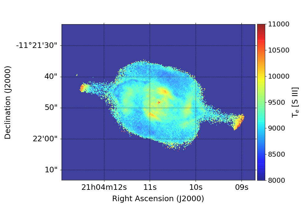
Figure 9: Illustrative output maps of the satellite code: c(H $\beta$) (upper), $N_{e}$ (middle) and $T_{e}$ (lower panel).

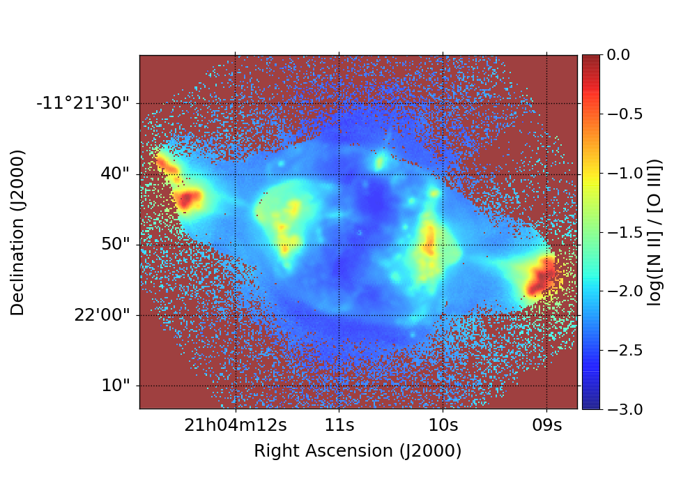
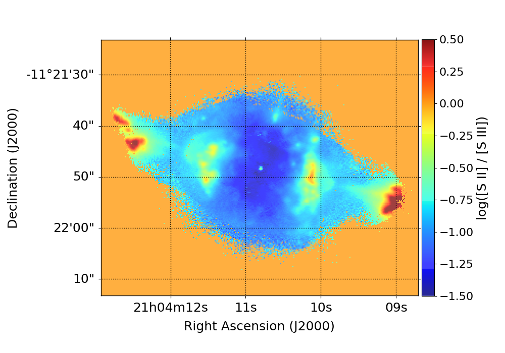
Figure 10: Illustrative output maps of the satellite code: log([N ii](6548+6584)/[O iii](4959+5007)) (upper) and log([S ii](6716+6731)/[S iii](6312+9069)) (lower panel) line ratios.

An analysis on the $T_{e}$ and $N_{e}$ between the different sub-structures and the entire nebula confirms the systematical lower electronic densities found in LISs compared to the main nebula and comparable electronic temperatures (e.g., Goncalves2003; Goncalves2009; Akras2016). The spectroscopic analysis of the specific regions/sub-structures shows a reasonable agreement with previous studies and verifies the performance of the satellite code. The larger discrepancy is found in $N_{e}$[Cl iii] for the pseudo-slit 10. We argue that the value of 1300 cm${}^{-3}$ Goncalves2003 is a typo as the [Cl iii] $\lambda$5517/$\lambda$5538 line ratio is very close to the value computed by satellite. Differences in abundances are mainly related to the $T_{e}$/$N_{e}$ diagnostics and the atomic data.

3.4 2D analysis module

Regarding the 2D analysis module, it allows us to study the entire nebula in both spatial directions simultaneously and explore the distribution of the physical parameters. In Figs 9 and 10, we present as illustrative examples the maps of c(H $\beta$), $T_{e}$, and $N_{e}$ as well as the log([N ii]/[O iii]) and log([S ii]/[S iii]) line ratios maps selected from a list of available line ratios. c(H $\beta$) map displays a filamentary structure in the inner nebula with enhanced extinction at the knots (see also fig. 1 in Walsh2016). It is evident that c(H $\beta$) is not smooth throughout the nebula and varies from 0.1 up to 0.3.

Table 3: Optical emission line fluxes from specific pseudo-slits or nebular regions.

Ion	I${}_{S_{F}}$	I${}_{W_{F})}$	I${}_{F}$	I${}_{S_{K1}}$	I${}_{G_{K1}}$	I${}_{S_{K4}}$	I${}_{G_{K4}}$	I${}_{S_{R1}}$	I${}_{G_{R1}}$	I${}_{S_{Neb}}$	I${}_{G_{Neb}}$
	p-slit 1	p-slit 1	slit 1	reg. 2	reg. 2	reg. 9	reg. 9	reg. 5	reg. 5	p-slit 10	slit 10
He ii 4686 Å	-	-	-	-	0.99	-	1.21	-	25.6	-	15.6
H i 4861 Å	100	100	100	100	100	100	100	100	100	100	100
[O iii] 4959 Å	385	388	388	395	428	429	454	380	405	390	421
[N i] 5199 Å	0.048	-	0.089	4.11	6.06	4.10	2.82	0.005	-	0.143	0.11
He ii 5412 Å	1.32	1.1	1.16	0.008	-	0.003	-	1.94	1.48	1.19	1.12
[Cl iii] 5517 Å	0.435	0.5	0.454	0.860	-	0.932	1.03	0.377	0.46	0.566	0.58
[Cl iii] 5538 Å	0.539	0.6	0.546	0.796	-	0.797	0.96	0.476	0.57	0.674	0.68
[N ii] 5755 Å	0.336	-	0.395	5.21	6.95	5.38	4.19	0.187	0.15	0.530	0.5
He i 5876 Å	14.6	-	14.4	16.4	20.3	16.2	16.2	13.8	15.0	14.8	15.7
[O i] 6300 Å	0.355	0.4	0.553	25.2	31.0	21.7	14.8	0.013	-	1.01	1.06
[S iii] 6312 Å	1.39	1.4	1.39	3.07	4.29	3.39	3.59	1.19	1.41	1.73	1.86
H i 6563 Å	288	-	266	290	394	290	224	291	312	291	313
[N ii] 6584 Å	14.3	14.7	15.6	324	397	330	217	5.05	7.93	26.5	30.2
He i 6678 Å	3.88	4.0	3.68	4.4	8.41	4.40	3.57	3.71	4.35	3.93	4.46
[S ii] 6717 Å	1.28	1.4	1.38	31.4	41.4	36.8	26.1	0.458	0.54	2.50	2.63
[S ii] 6731 Å	2.18	2.3	2.28	43.8	57.4	45.3	32.0	0.818	0.95	4.12	4.34
[Ar iii] 7136 Å	15.7	-	14.9	27.4	-	29.2	-	14.5	-	17.5	-
[O ii] 7320 Å	1.36	1.3:	1.19	8.56	-	7.45	-	1.09	-	1.63	-
[O ii] 7330 Å	1.17	1.1	1.11	7.19	-	6.36	-	0.943	-	1.38	-
[S iii] 9069 Å	24.5	25.2	23.2	48.7	-	51.3	-	19.7	-	29.9	-
F(H $\beta$)(10${}^{-13}$)	199	-	-	1.21	1.05	0.78	1.28	22.6	30.7	158	188
c(H $\beta$)	0.177	-	0.174	0.158	0.16	0.16	0.16	0.165	0.16	0.165	0.16
Te[N ii]	11724	-	10780	10191	11000	10309	11700	14735	10400	10989	10300
Te[S iii]	9272	-	11500	9677	9600${}^{b}$	9877	10400${}^{b}$	9453	10000${}^{b}$	9293	10100${}^{b}$
Ne[S ii]	3661	-	4100	1628	2000	1059	1300	4959	5500	3100	4000
Ne[Cl iii]	5150	-	3600	1862	-	1249	1900	5475	5200	4557	1300
He+(5876)/H+	0.093	-	0.103	0.11	0.10	0.11	0.096	0.074	0.095	0.096	0.098
He+(6678)/H+	0.088	-	0.095	0.11	-	0.11	-	0.070	-	0.091	-
He^++(5412)/H+	0.014	-	0.013${}^{c}$	0.00008	-	0.00003	-	0.021	0.012${}^{c}$	0.013	0.013${}^{c}$
He/H	0.109	-	0.112	0.11	0.10	0.11	0.096	0.094	0.108	0.106	0.111
N${}^{0}$/H+ (-7)	1.13	-	0.84	96.8	87.0	75.3	27.0	0.07	-	3.72	2.7
N+/H+ (-6)	2.02	-	2.73	62.7	50.0	61.6	23.8	43.7	1.10	4.31	4.45
ICF(N)${}^{a}$	67.3/-	-	-	3.94/7.06	7.8	4.13/8.44	10.6	264/-	64.7	38.0/-	38.2
N/H${}^{a}$ (-5)	13.6/-	-	7.01${}^{d}$	24.7/44.3	38.0	25.5/52.1	25.0	11.6/-	7.0	16.5/-	17.0
O${}^{0}$/H+ (-6)	0.39	-	0.84	44.4	45.0	36.6	18.0	0.07	0.5	1.36	1.71
O+/H+ (-5)	0.87	-	1.99	15.6	7.5	14.9	4.2	21.5	0.7	1.53	1.2
O^++/H+ (-4)	5.20	-	3.23	4.59	5.12	4.65	4.1	4.80	4.12	5.22	4.21
ICF(O)${}^{a}$	1.10/1.09	-	1.086	1.0/1.0	1.0	1.09/1.08	1.00	1.18/1.16	1.08	1.09/1.08	1.08
O/H${}^{a}$ (-4)	5.83/5.75	-	3.6	6.16/6.16	5.8	5.86/5.79	4.5	5.70/5.59	4.5	5.86/5.79	4.71
S+/H+ (-7)	1.06	-	1.19	24.0	22.1	23.2	10.1	0.28	0.44	2.17	2.09
S^++/H+ (-6)	4.18	-	2.26	7.74	7.45	7.86	4.8	3.24	2.1	5.11	3.3
ICF(S)${}^{a}$	2.83/-	-	?	1.20/1.09	1.43	1.13/1.11	1.57	4.46/-	2.79	2.36/-	2.35
S/H${}^{a}$ (-6)	12.2/-	-	13.0	12.1/11.1	13.9	12.3/11.3	9.3	14.6/-	6.1	12.5/-	8.3
Cl^++/H+ (-8)	8.65	-	5.51	11.8	-	11.3	-	7.15	-	10.8	-
ICF(Cl)${}^{a}$	-/2.92${}^{e}$	-	?	-/-	-	-/-	-	-/3.90${}^{e}$	-	-/2.37	-
Cl/H${}^{a}$ (-7)	-/2.36${}^{e}$	-	1.93	-/-	-	-/-	-	-/2.79${}^{e}$	-	-/2.55	-
Ar^++/H+ (-6)	1.56	-	1.03	2.43	-	2.46	-	1.36	-	1.71	-
ICF(Ar)${}^{a}$	1.87/-	-	?	1.87/1.19	-	1.87/1.21	-	1.87/-	-	1.87/-	-
Ar/H${}^{a}$ (-6)	2.92/-	-	2.57	4.55/2.91	-	4.61/2.98	-	2.54/-	-	3.20/-	-

I is the intensity of the lines in the scale where H$\beta$ = 100. The The indices S, W, F, and G point out the results obtained with satellite or from previous studies: (Walsh2018), (Fang2011) and (Goncalves2003). The indices K1, K4, R and Neb correspond to the sub-structures and total nebula based on Goncalves2003. ${}^{a}$ Elemental abundances are provided using the ICFs from Kingsburgh1994K (left) and Delgado2014 (right), ${}^{b}$ These values correspond to the Te[O iii] values, ${}^{c}$He ii 4686Å line is used for the computation of the ionic abundance, ${}^{d}$ Recombination and collisionally excited lines from UV, optical and IR were used to determine the abundance, ${}^{e}$ satellite does not calculate/provide the total abundance and ICF of Cl because it lies outside the range of validity. “?”= unknown value.

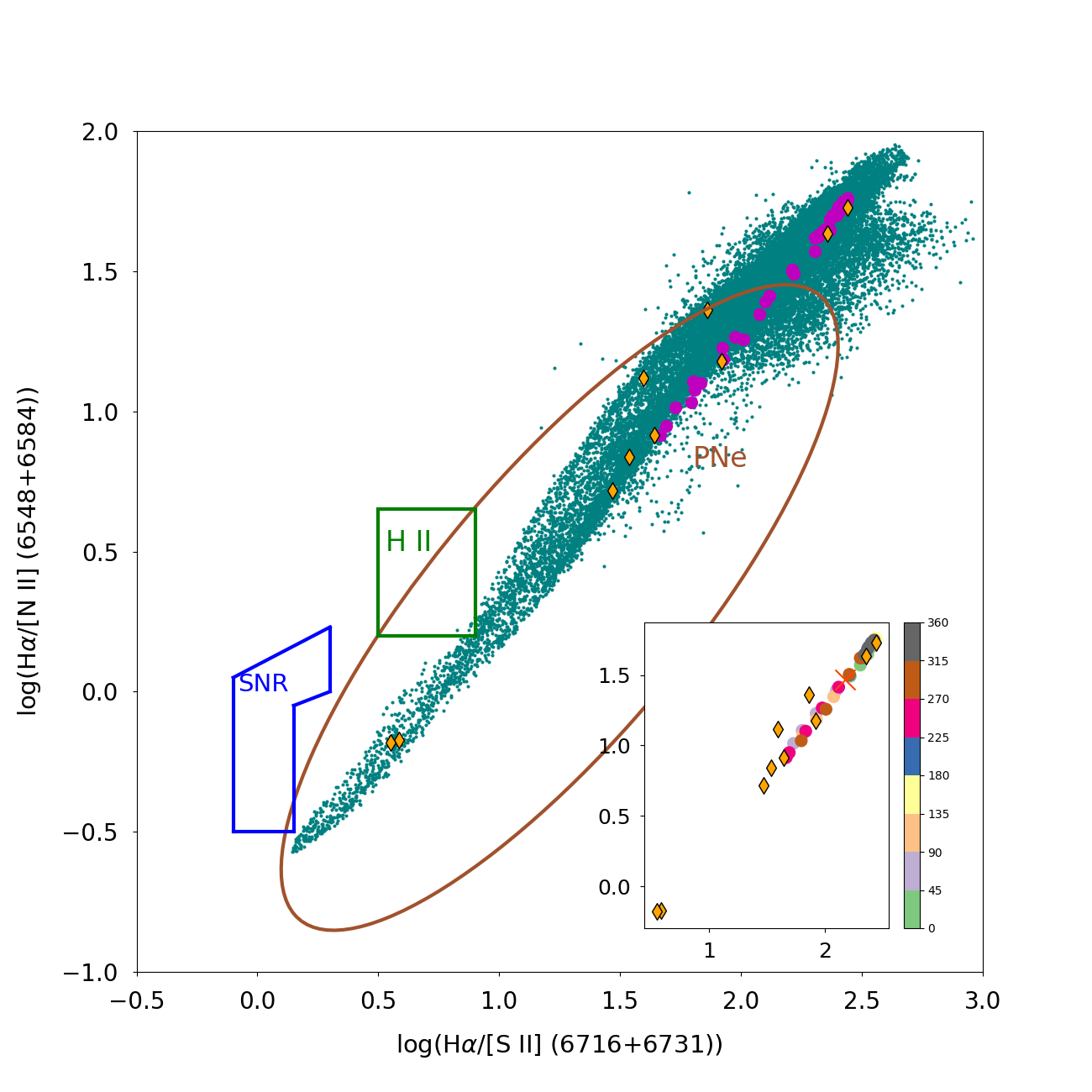
Figure 11: Log(H $\alpha$/[S ii] 6716+6731) versus Log(H $\alpha$/[N ii] 6548+6584) diagnostic diagram of NGC 7009 as a representative example. Cyan dots correspond to the values of individual spaxels, pink circles and yellow diamonds show the values obtained from the pseudo-slits of the rotational analysis module with position angles from 0 to 360 degrees with 10 degrees step and the values from the 10 pseudo-slits in the specific slits analysis module, respectively. The inset plot illustrate the variation of the line ratios with position angles of the pseudo-slits. The regimes of the PNe, H ii regions and supernova remnants are also drawn (Sabbadin1977; Riesgo2006; Frew2010; Sabin2013).

Besides the maps, the 2D analysis module also provides emission line diagnostic diagrams, selected by the user from a predefined list. Fig. 11 illustrates the common diagnostic diagram log(H $\alpha$/[S ii]) versus log(H $\alpha$/[N ii]). The line ratio values from the individual spaxels are plotted as cyan points, the pseudo-slit spectra from the rotation analysis module as purple circles in the main plot or colored circles in the inset plot (color bar corresponds to the PA of the pseudo-slits) and those from the specific slits analysis module as yellow diamonds.

Table 4: Statistical results of NGC 7009 MUSE datacube.

Parameter	Num. of pix.	5% value	25% value	50%	75% value	95% value	mean	SD
c(H $\beta$)	40841	0.011	0.053	0.108	0.145	0.193	0.105	0.065
Te(NII6548_84)_Ne(SII6716_31)	19554	10000	10900	12100	13500	18700	13000	3200
Ne(SII6716_31)_Te(NII6548_84)	19554	828	1550	2490	3660	6870	3040	2090
Te(SIII6312_9069)_Ne(SII6716_31)	26658	8770	9000	9220	9480	10800	9420	749
Ne(SII6716_31)_Te(SIII6312_9069)	26658	615	1160	1930	3030	6100	2570	2300
Te(SIII6312_9069)_Ne(ClIII5517_38)	17305	8780	8950	9130	9270	9700	9170	301
Ne(ClIII5517_38)_Te(SIII6312_9069)	17305	1010	2060	3220	4610	7070	3610	2040
log(He i 5876/H $\alpha$)	40017	-1.33	-1.27	-1.26	-1.25	-1.22	-1.26	0.04
log(He ii 5412/H $\beta$)	14528	-3.05	-2.88	-2.53	-2.13	-1.64	-2.44	0.48
log(He i 5876/He ii 5412)	14526	0.76	1.22	1.74	2.05	2.26	1.63	0.51
log([N ii] 6584/H $\alpha$)	40228	-1.87	-1.70	-1.55	-1.42	-0.69	-1.46	0.38
log(([N ii] 6548,6584)/([O iii] 4959,5007))	40214	-2.52	-2.39	-2.25	-2.11	-1.35	-2.15	0.38
log([N i] 5200/H $\beta$)	5232	-3.22	-3.06	-2.64	-2.23	-1.10	-2.48	0.66
log(([S ii] 6716,6731)/H $\alpha$)	28808	-2.46	-2.25	-2.08	-1.90	-1.14	-1.98	0.42
log([S ii] 6716/[S ii] 6731)	28808	-0.29	-0.23	-0.17	-0.11	0.0001	-0.16	0.09
log(([S ii] 6716,6731)/([S iii] 6312,9069))	27687	-1.27	-1.06	-0.91	-0.82	-0.32	-0.88	0.30
log[O i] 6300/H $\alpha$)	11752	-3.80	-3.71	-3.16	-2.62	-1.25	-2.95	0.83
log([O iii] 5007/H $\beta$)	40734	1.05	1.07	1.12	1.20	1.28	1.14	0.08
log(([O ii] 7320,7330)/([O iii] 4959,5007))	22637	-3.15	-3.06	-2.97	-2.86	-2.45	-2.91	0.24
log(([Cl iii] 5517,5538)/H $\beta$)	18176	-2.10	-2.03	-1.97	-1.92	-1.80	-1.96	0.09
abundance (He i 5876Å)	17305	0.088	0.102	0.108	0.110	0.113	0.105	0.008
abundance (He i 6678Å)	17305	0.083	0.096	0.103	0.105	0.109	0.099	0.008
abundance (He ii 5412Å)	14052	9.39e-04	1.39e-03	3.09e-03	8.16e-03	2.48e-02	7.21e-03	8.13e-03
abundance ([O i] 6300 Å)	8948	1.14e-07	1.47e-07	2.83e-07	7.71e-07	1.75e-05	4.32e-06	1.61e-05
abundance ([O ii] 7320 Å)	17298	1.69e-05	2.40e-05	2.90e-05	3.30e-05	6.60e-05	3.49e-05	3.15e-05
abundance ([O ii] 7330 Å)	17285	1.82e-05	2.59e-05	3.14e-05	3.56e-05	6.48e-05	3.72e-05	3.29e-05
abundance ([O iii] 5007 Å)	17305	4.44e-04	5.32e-04	5.73e-04	6.01e-04	6.62e-04	5.67e-04	6.85e-05
abundance ([N i] 5199 Å)	3646	3.22e-07	4.10e-07	6.73e-07	1.52e-06	1.53e-05	3.05e-06	7.26e-06
abundance ([N ii] 5755 Å)	16705	2.64e-06	3.29e-06	4.36e-06	5.96e-06	2.42e-05	8.37e-06	1.52e-05
abundance ([N ii] 6584 Å)	17305	8.35e-07	1.34e-06	2.03e-06	3.21e-06	1.85e-05	5.69e-06	1.44e-05
abundance ([S ii] 6717 Å)	17301	5.17e-08	8.23e-08	1.29e-07	2.15e-07	1.00e-06	3.18e-07	6.91e-07
abundance ([S ii] 6731 Å)	17305	5.06e-08	7.97e-08	1.20e-07	2.00e-07	9.18e-07	2.93e-07	6.11e-07
abundance ([S iii] 6312 Å)	17305	2.63e-06	3.35e-06	4.06e-06	5.00e-06	7.48e-06	4.49e-06	1.55e-06
abundance ([S iii] 9069 Å)	17305	2.63e-06	3.35e-06	4.06e-06	5.00e-06	7.48e-06	4.49e-06	1.55e-06
abundance ([Cl iii] 5517 Å)	17305	6.57e-08	8.47e-08	9.83e-08	1.10e-07	1.36e-07	9.98e-08	2.36e-08
abundance ([Cl iii] 5538 Å)	17305	6.57e-08	8.47e-08	9.83e-08	1.10e-07	1.36e-07	9.98e-08	2.36e-08
abundance ([Ar iii] 7136 Å)	17305	1.16e-06	1.40e-06	1.60e-06	1.79e-06	2.25e-06	1.65e-06	3.37e-07

50% percentiles corresponds to the median.

The majority of the spaxels as well as some pseudo-slits from the rotation analysis and specific slit analysis modules (pseudo-slits 1 and 10 that cover the entire nebula from one side to the other) have values up to log(H $\alpha$/[S ii])$\sim$2.5 and log(H $\alpha$/[N ii])$\sim$1.75 lying outside the 85 percent confidence level ellipse (Riesgo2006). This clearly demonstrates that the regime of PNe in the STB diagnostic diagram should be updated by covering higher H $\alpha$/[S ii] and H $\alpha$/[N ii] line ratios. The same conclusion has been reached from the prediction of 1D photo-ionization models (see Fig. 5 in Akras2020a).

Moreover, there is a non-negligible number of spaxels with moderate or even low values (log(H $\alpha$/[S ii])<1.0 and log(H $\alpha$/[N ii])<0.25) close to the loci of H ii regions and SNRs (Frew2010; Sabin2013) whereas pseudo-slits from the rotation analysis and specific slit analysis modules do not display such low ratios. Interestingly, two pseudo-slits from the specific slit analysis module (pseudo-slits 2 and 9) have the lowest values (log(H $\alpha$/[S ii])$\sim$0.5 and log(H $\alpha$/[N ii])$\sim$ -0.5) and correspond to the extracted windows from the two LISs/knots K1 and K4. Our mean values of the H $\alpha$/[S ii] and H $\alpha$/[N ii]  ratios for the K1 and K4 knots agree with the results from HST imaging Phillips2010 but we do not observe the same distribution for individual spaxels. In particular, HST data display H $\alpha$/[S ii] and H $\alpha$/[N ii]  ratio values well distributed in the SNRs regime (see fig. 19 in Phillips2010) while the distribution of the individual MUSE spaxels is within the PNe regime. Hence, we argue that any contribution of shocks in the knots of NGC 7009 is indistinguishable.

It is evident that line ratios can vary significantly from one sub-structure to another. The main nebula of NGC 7009 is certainly UV dominated and all its physical properties as well as emission line ratios can be explained from the strong UV radiation field of its central star. However, there are sub-structures like K1 to K4 LISs that diverge from the main bulk (Fig. 11). To explain the large divergence of line ratios in different sub-structures in the nebula with comparable physical parameters (Table 3), a high density gas should be considered in these sub-structures. The detection of H${}_{2}$ emission from the LISs in NGC 7009 (Akras2020b) supports the presence of a high density gas. The enhancement of low-ionisation emission such as [N ii], [O i] emission lines in conjunction with the H${}_{2}$ emission implies the presence of mini-photodissociation regions (PDRs). Furthermore, the detection of an emission at 8727Å very likely associated with the red-[C i] line (Akras et al. 2021 in preparation), found in PDRs (Burton1992, e.g.) and PNe (Liu1995CI), further supports the scenario that the enhanced emission from the low-ionization species found in the LISs of NGC 7009 originate from the partially ionized gas of mini-PDRs rather than shock-heated gas.

satellite also calculates the mean value, standard deviation and the percentiles of 5%, 25% (Q1), 50% (median), 75% (Q3), 95% for each parameter with 2D maps constructed, such as c(H $\beta$), $T_{e}$, and $N_{e}$, ionic abundances and line ratios (Table 4) (see also, Monreal2020).

4 The case study of NGC 7009 with deeper MUSE data

Besides the SV MUSE data, deeper observations were also obtained in visitor mode on 07 July 2016 (097.D-0241(A), PI: R. L. M. Corradi; hereafter Cor MUSE data) using the extended mode. Short and long observations were obtained with exposure times of 30 and 150 sec, respectively. For the long exposure observations ten frames were obtained at different position angles resulting in total integrated times of 1500 sec. The DIMM seeing during the observations varied from 0.8 to 1.2 arcsec and the airmass changed from 1.126 to 1.357. Unfortunately, these observations were not carried out under photometric conditions due to the presence of thin cirrus. For consistency with the SV data, we found that the short and long exposure line maps of the Cor MUSE datacubes should be multiplied by 0.46$\pm$0.05 and 2.4$\pm$0.1, respectively. This introduces an extra uncertainty on the analysis but it is valuable to verify the performance of satellite using the flux maps from a second datacube and an independent reduction and emission line fitting.

Line intensities, physical parameters (c(H $\beta$), T${}_{\rm e}$, N${}_{\rm e}$) and abundances computed from the pseudo-slits 1, 10 (Fig. 3) and the entire nebula (2310 square arcseconds) obtained with the satellite code from the SV and Cor MUSE data are listed in Table 5. The comparison of the line intensities between the two datacubes is displayed in Fig. 12. A reasonable matching is also found for all the nebular parameters. Only the extinction coefficient exhibits an unexpected mismatch of the order or 25 percent, due to the non-photometric night. Thus, within the involved uncertainties, the results validate the specific slit analysis module of the satellite code for the spectroscopic analysis of specific regions or sub-structures in PNe such as knots.

The results from the rotation analysis and radial analysis modules are also consistent between the two datasets. All the nebula parameters show the same behaviour with the PA of the pseudo-slits and similar absolute values (not presented here). The high T${}_{\rm e}$[N ii] values at the PAs of 0, 150 and 320 degrees are found again with the Cor MUSE data. The radial profiles of the nebular parameter are also comparable. T${}_{\rm e}$[N ii] is higher at the central region of the nebula and decreases for larger distance while T${}_{\rm e}$[S iii] is nearly constant. As for the electron density, very small differences are found.

For the 2D analysis module, the results of the statistical analysis of the Cor MUSE maps, for instance the mean values, standard deviations and the 5%, 25% (Q1), 50% (median), 75% (Q3) and 95% percentiles provide an overall consistency between the two set datacubes.

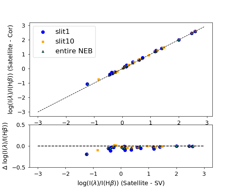
Figure 12: Comparison of the line ratios relative to H$\beta$=100 obtained from the pseudo-slits 1, 10 and the entire nebula of NGC 7009 from two MUSE datacubes using satellite: science verification MUSE data (SV), (Walsh2018) and the Cor MUSE data (097.D-0241(A), PI: R. L. M. Corradi).

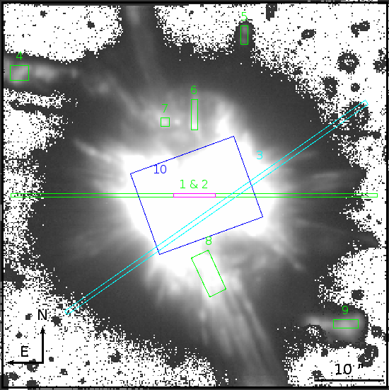
Figure 13: 10 slits/regions selected for the spectroscopic analysis of specific slits with satellite are overlaid on the [N ii] $\lambda$6584 line map of NGC 6778. North is up east to the left.

Table 5: Comparison between optical emission line fluxes and derived quantities from specific slits between SV and Cor MUSE data of NGC 7009.

Ion	I${}_{S_{F}}$ (SV)	I${}_{S_{F}}$ (Cor)	I${}_{S_{Neb}}$ (SV)	I${}_{S_{Neb}}$ (Cor)	I${}_{S_{entire}}$ (SV)	I${}_{S_{entire}}$ (Cor)
	p-slit 1	p-slit 1	p-slit 10	p-slit 10	2310 arcsec${}^{2}$	2310 arcsec${}^{2}$
He ii 4686 Å	-	17.5	-	16.4	-	14.3
H i 4861 Å	100	100	100	100	100	100
[O iii] 4959 Å	385	391	390	396	388	395
[N i] 5199 Å	0.048	0.087	0.143	0.177	0.058	0.091
He ii 5412 Å	1.32	1.35	1.20	1.24	1.04	1.10
[Cl iii] 5517 Å	0.435	0.468	0.566	0.538	0.468	0.488
[Cl iii] 5538 Å	0.539	0.578	0.674	0.645	0.554	0.575
[N ii] 5755 Å	0.336	0.408	0.530	0.540	0.330	0.355
He i 5876 Å	14.6	15.4	14.8	15.6	14.9	15.7
[O i] 6300 Å	0.355	0.544	1.01	1.05	0.411	0.450
[S iii] 6312 Å	1.39	1.60	1.73	1.86	1.39	1.50
[N ii] 6548 Å	4.88	5.82	8.85	8.82	4.89	4.88
H i 6563 Å	288	289	291	289	288	289
[N ii] 6584 Å	14.3	18.1	26.5	27.3	14.6	15.2
He i 6678 Å	3.88	4.12	3.93	4.20	3.98	4.24
[S ii] 6717 Å	1.28	1.71	2.50	2.70	1.39	1.54
[S ii] 6731 Å	2.18	2.88	4.12	4.41	2.32	2.53
[Ar iii] 7136 Å	15.7	17.3	17.5	18.6	15.5	16.5
[O ii] 7320 Å	1.36	1.58	1.63	1.78	1.29	1.41
[O ii] 7330 Å	1.17	1.35	1.38	1.51	1.11	1.21
[S iii] 9069 Å	24.5	26.3	29.9	30.3	24.8	24.9
F(H $\beta$)(10${}^{-13}$)	199	208	158	159	1458	1469
c(H $\beta$)	0.170	0.221	0.165	0.211	0.166	0.218
Te[N ii]	11724	11578	10989	10980	11547	11822
Te[S iii]	9272	9516	9293	9566	9219	9498
Ne[S ii]	3661	3493	3100	2999	3333	3167
Ne[Cl iii]	5150	5127	4577	4776	4648	4435
He+(5876)/H+	0.093	0.098	0.096	0.102	0.096	0.10
He+(6678)/H+	0.088	0.094	0.091	0.098	0.091	0.096
He^++(5412)/H+	0.014	0.014${}^{b}$	0.013	0.013${}^{b}$	0.011	0.017${}^{b}$
He/H	0.109	0.111	0.106	0.113	0.105	0.107
N${}^{0}$/H+ (-7)	1.13	2.05	3.72	4.50	1.34	1.88
N+/H+ (-6)	2.02	2.57	4.31	4.41	2.12	2.06
ICF(N)${}^{a}$	67.3/-	40.7/-	38.0/-	31.4/-	64.1/-	63.1/-
N/H${}^{a}$ (-5)	13.6/-	12.9/-	16.5/-	13.9/-	13.7/-	13.8/-
O+/H+ (-5)	0.87	1.09	1.53	1.72	0.92	0.95
O^++/H+ (-4)	5.20	4.82	5.22	4.79	5.35	4.90
ICF(O)${}^{a}$	1.10/1.09	1.09/1.08	1.09/1.08	1.09/1.07	1.08/1.07	1.08/1.07
O/H${}^{a}$ (-4)	5.83/5.75	5.41/5.34	5.86/5.79	5.40/5.33	5.87/5.81	5.36/5.30
S+/H+ (-7)	1.06	1.41	2.17	2.32	1.13	1.15
S^++/H+ (-6)	4.18	4.27	5.11	4.86	4.30	4.07
ICF(S)${}^{a}$	2.83/-	2.56/-	2.36/-	2.21/-	2.78/-	2.77/-
S/H${}^{a}$ (-6)	12.2/-	11.3/-	12.5/-	11.3/-	12.3/-	11.6/-
Cl^++/H+ (-8)	8.65	8.55	10.8	9.41	9.10	8.60
ICF(Cl)${}^{a}$	-/2.92${}^{c}$	-/2.53	-/2.37	-/2.26	-/2.65	-/2.65
Cl/H${}^{a}$ (-7)	-/2.36${}^{c}$	-/2.17	-/2.55	-/2.13	-/2.42	-/2.23
Ar^++/H+ (-6)	1.56	1.61	1.71	1.71	1.57	1.55
ICF(Ar)${}^{a}$	1.87/-	1.87/-	1.87/-	1.87/-	1.87/-	1.87/-
Ar/H${}^{a}$ (-6)	2.92/-	3.01/-	3.20/-	3.20/-	2.93/-	2.89/-

${}^{a}$ Elemental abundances are provided using the ICFs from Kingsburgh1994K (left) and Delgado2014 (right).

${}^{b}$ He ii 4686Å line is used for the computation of the ionic abundance.

${}^{c}$ satellite does not calculate/provide the total abundance and ICF of Cl because the criteria are not satisfied.

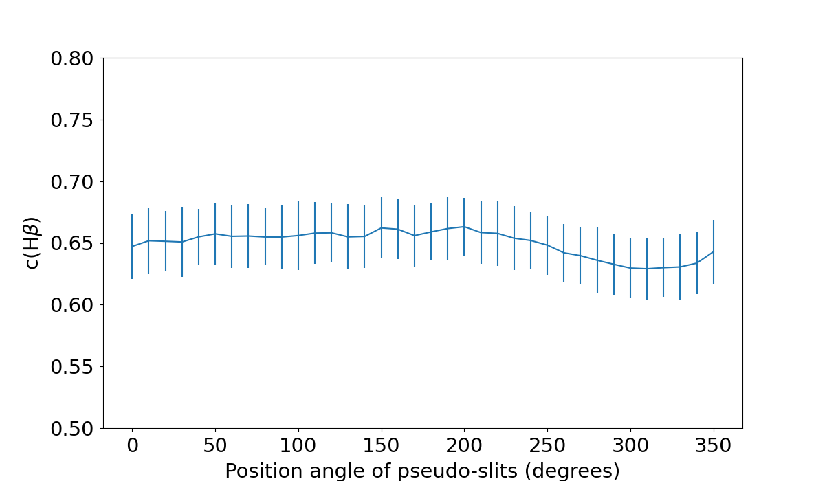
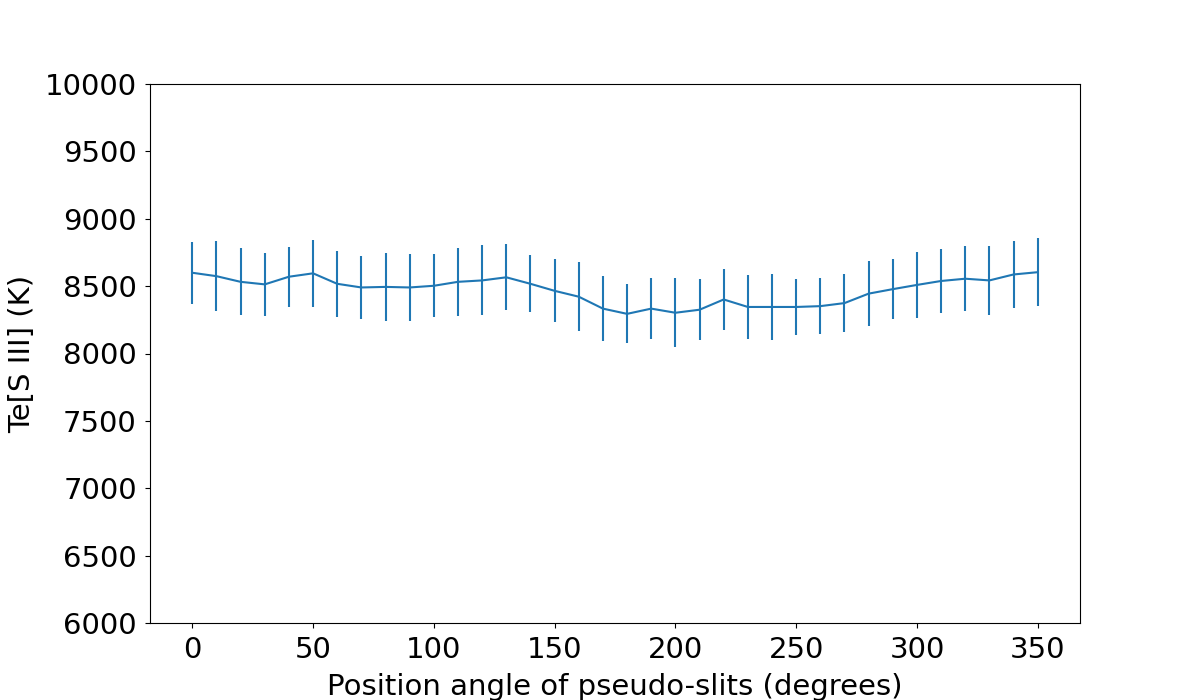
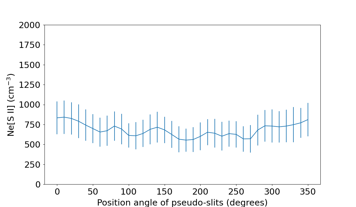
Figure 14: c(H$\beta$), T${}_{\rm e}$[S iii] and N${}_{\rm e}$[S ii] as functions of the pseudo-slit position angles for NGC 6778

5 The case study of NGC 6778 with Cor MUSE data

In this section, we present the spectroscopic analysis of the planetary nebula NGC 6778 employing the satellite code and MUSE data (097.D-0241(A), PI: R. L. M. Corradi). NGC 6778 has a complex morphology with a bright waist, a number of low-ionization knots and two pairs of collimated jets (Guerrero2012). What makes this nebula an intriguing object is its central star which has been found to be a close binary system with a period of $\sim$0.15 days (Miszalski2011). Binary systems in PNe have been linked with a high abundance discrepancy factor and NGC 6778 is one of them (adf=20, Jones2016).

Recent data from OSIRIS Blue Tunable Filter (GTC) and VIMOS IFU (VLT) have revealed a significant difference in the spatial distribution between the O ii 4649+50Å  optical recombination lines (ORLs) and the collisionally excited [O iii] $\lambda$5007 line (GarciaRojas2016). Interestingly, the auroral [O iii] $\lambda$4363 line displays the same spatial distribution as the O ii recombination line resulting in questionable T${}_{\rm e}$ (GomezLlanos2020). These results make NGC 6778 an ideal target for a 2D imaging spectroscopic analysis with deep MUSE data. A full presentation of the data and spatial analysis of the complete MUSE data set of NGC 6778, including C ii, O ii and N ii ORLs has been presented in Garciarojas2022. In this work with satellite, we focus on the spectroscopic analysis of the nebula using the bright collisionally excited lines (CELs) and H/He recombination lines.

Figure 15: Ionic and total N (upper panel) and O (middle panel) abundances of NGC 6778 as well a N/O ratio (lower panel) as a function of the pseudo-slit position angles. The total abundances is computed using the ICFs schemes from Kingsburgh1994K and Delgado2014.

Figure 16: Ionic and total S (upper panel) abundances and S/O ratio (lower panel) of NGC 6778 a function of the pseudo-slit position angles. The total abundances is computed using the ICFs schemes from Kingsburgh1994K and Delgado2014. The ionic abundances derived from [S ii] $\lambda$6716 and $\lambda$6731, and [S iii] $\lambda$6312 and $\lambda$9069 emission lines are very similar which makes one overlays the other.

Fig. 13 illustrates the 10 pseudo-slits/regions selected for the spectroscopic exploration. The magenta slit (number 1) corresponds to the slit position from Dufour2015. The green pseudo-slit 2 has the same width as the pseudo-slit 1, but it is 60 arcsec longer, in order to cover the nebula from one side to the other and compare the results with those from the pseudo-slit 1 centred only on the inner zone. The cyan pseudo-slit 3 corresponds to the slit of Jones2016 (PA=$-$55 degrees). Pseudo-slits 4 to 9 (green colour) cover a number of LISs distributed throughout the nebula. Finally, pseudo-slit 10 (blue colour) covers the whole central region of NGC 6778.

In Table 6, we present the interstellar extinction corrected line intensities for the pseudo-slits as well as the integrated spectrum for an area of 1602 square arcsec. The spectra from the pseudo-slits 1 and 3 are compared with the observations in Dufour2015 and Jones2016, respectively, and a very good agreement is found for the majority of the lines and physical parameters (c(H $\beta$), T${}_{\rm e}$ and N${}_{\rm e}$). The integrated F(H $\beta$) flux of the whole nebula is being 5.72$\times$10${}^{-12}$ erg s${}^{-1}$ cm${}^{-2}$, in reasonable agreement with the value of 6.92$\times$10${}^{-12}$ erg s${}^{-1}$ cm${}^{-2}$ found by Acker1992.

The extinction coefficient is found to be 0.65 with a standard deviation of 0.02 between the values reported by Dufour2015 and Jones2016. T${}_{\rm e}$[S iii] and N${}_{\rm e}$[S ii] measured for the pseudo-slits vary from 8300 to 8600 K and from 550 to 850 cm${}^{-3}$, respectively, in agreement with the literature.

Chemical abundances are provided only by Jones2016 and can be compared with those obtained for the pseudo-slit 3. Despite the agreement in the line intensities and T${}_{\rm e}$/N${}_{\rm e}$, a significant difference in the chemical abundances is found. In particular, we find slightly higher He, twice higher O and S, half N and comparable or half Ar abundances depending on the ICF. This discrepancy in abundances is associated to a combination of the different extinction, physical conditions, atomic data sets and ICFs adopted. A more detailed analysis of such differences has been presented in Garciarojas2022. All chemical abundances derived from the pseudo-slits and the central region (Table 6) show small variations, within their uncertainties.

Table 6: Optical emission line intensities from the specific slit task of NGC 6778

Ion	I${}_{S_{D})}$	I${}_{D}$	I${}_{S_{D}}~{}\rm{ext^{{\dagger}}}$	I${}_{S_{J}}$	I${}_{J}$	I${}_{S}$	I${}_{S}$	I${}_{S}$	I${}_{S}$	I${}_{S}$	I${}_{S}^{{\dagger}{\dagger}}$
	p-slit 1	slit 1	p-slit 2	p-slit 3	slit 3	p-slit 4	p-slit 6	p-slit 8	p-slit 9	p-slit 10	1602 arc${}^{2}$
He ii 4686 Å	17.4	19.8	8.26	4.07	6.50	13.4	1.66	0.624	11.4	5.69	5.10
H i 4861 Å	100	100	100	100	100	100	100	100	100	100	100
[O iii] 4959 Å	171	171	171	169	171.11	99.5	119	141	92.3	171	167
[N i] 5199 Å	2.12	-	2.69	2.46	-	15.8	1.60	3.50	13.5	2.99	3.15
[Cl iii] 5517 Å	0.548	-	0.646	0.652	-	5.84	0.610	0.672	6.02	0.633	0.715
[Cl iii] 5538 Å	0.465	-	0.556	0.553	-	6.08	0.489	0.557	5.65	0.544	0.615
[N ii] 5755 Å	2.58	-	2.76	2.40	-	11.2	1.34	2.39	9.98	2.91	2.87
He i 5876 Å	23.0	26.1	23.2	23.4	22.12	27.0	23.7	23.3	25.2	23.3	23.4
[O i] 6300 Å	3.34	-	4.41	3.81	3.69	32.1	1.66	5.15	24.9	4.97	5.05
[S iii] 6312 Å	1.09	-	1.19	1.11	1.05	4.34	0.695	0.905	2.64	1.21	1.20
H i 6563 Å	296	286	296	296	289.88	297	297	297	296	297	296
[N ii] 6584 Å	195	153	257	229	226.65	879	142	302	981	282	279
He i 6678 Å	6.57	8.54	6.65	6.72	6.61	9.41	6.79	6.64	7.90	6.69	6.71
[S ii] 6717 Å	14.3	12.9	19.3	17.1	16.92	59.7	12.1	24.78	64.3	20.8	21.1
[S ii] 6731 Å	16.3	14.7	21.0	18.1	18.00	44.9	11.1	23.7	48.9	23.1	22.6
[Ar iii] 7136 Å	14.6	11.0	16.8	16.4	-	19.6	13.2	17.1	20.2	17.4	17.3
[O ii] 7320 Å	3.14	-	2.58	2.30	-	4.99	1.25	1.56	4.52	2.51	2.29
[O ii] 7330 Å	2.54	-	2.08	1.88	-	8.39	1.13	1.26	4.99	2.04	1.20
[S iii] 9069 Å	23.7	17.7	27.6	27.3	-	18.1	21.6	22.8	20.5	28.4	27.8
F(H $\beta$)(10${}^{-14}$)	10.7	3.09	27.6	26.6	-	0.05	0.79	5.77	0.04	465	572
c(H $\beta$)	0.65	0.74	0.65	0.65	0.46	0.69	0.65	0.65	0.60	0.65	0.64
Te[N ii]	9524	10300${}^{a}$	8830	8769	8850${}^{b}$	9441	8472	7996	8704	8689	8697
Te[S iii]	8578	-	8388	8219	8800${}^{b}$	22454${}^{c}$	7591	8139	13945${}^{c}$	8329	8374
Ne[S ii]	781	919	661	586	590	90	318	380	100	685	610
Ne[Cl iii]	1179	-	1262	1156	-	3308	784	1014	2054	1249	1262
He+(5876)/H+	0.161	-	0.161	0.163	0.154	-	0.163	0.163	-	0.162	0.163
He+(6678)/H+	0.161	-	0.163	0.164	-	-	0.164	0.162	-	0.164	0.164
He^++(4686)/H+	0.014	-	0.007	0.003	-	-	0.013	0.001	-	0.001	0.004
He/H	0.175	-	0.169	0.167	0.159	-	0.165	0.163	-	0.167	0.168
N${}^{0}$/H+ (-6)	7.13	-	9.50	9.16	-	-	7.42	12.2	-	11.1	10.0
N+/H+ (-5)	5.99	-	8.48	7.99	5.55	-	6.37	1.09	-	9.58	9.31
ICF(N)	2.51/2.54	-	2.56/2.79	2.52/2.94	?	-	2.21/2.76	2.62/3.71	-	2.56/2.90	2.57/2.93
N/H (-4)	1.51/1.52	-	2.17/2.36	2.01/2.35	4.04	-	1.41/1.76	2.88/4.06	-	2.45/2.77	2.39/2.73
O${}^{0}$/H+ (-6)	12.0	-	17.4	16.0	-	-	11.1	22.9	-	20.1	20.2
O+/H+ (-4)	2.24	-	2.26	2.33	0.56	-	2.98	1.95	-	2.29	2.18
O^++/H+ (-4)	3.08	-	3.37	3.62	2.83	-	3.58	3.15	-	3.46	3.34
ICF(O)	1.06/1.05	-	1.03/1.02	1.01/1.01	?	-	1.00/1.00	1.00/1.00	-	1.02/1.02	1.02/1.01
O/H (-4)	5.63/5.58	-	5.78/5.76	6.14/6.12	3.39	-	6.60/6.59	5.11/5.11	-	5.86/5.84	5.58/5.57
S+/H+ (-6)	1.33	-	1.84	1.67	1.44	-	1.34	2.29	-	2.06	1.98
S^++/H+ (-6)	4.88	-	5.99	6.21	4.26	-	5.97	5.34	-	6.27	6.06
ICF(S)	1.09/1.02	-	1.09/1.01	1.09/1.01	?	-	1.06/1.0	1.09/1.01	-	1.09/1.0	1.09/1/00
S/H (-5)	0.68/0.0.63	-	0.85/0.78	0.86/0.78	0.34	-	0.78/0.71	0.84/0.76	-	0.91/0.83	0.88/0.80
Cl^++/H+ (-7)	1.04	-	1.33	1.43	-	-	1.75	1.51	-	1.34	1.49
ICF(Cl)	-/1.37	-	-/1.34	-/-	?	-	-/-	-/-	-	-/1.33	-/1.33
Cl/H (-7)	-/1.43	-	-/1.79	-/-	-	-	-/-	-/-	-	-/1.79	-/1.97
Ar^++/H+ (-6)	1.78	-	2.16	2.25	3.80	-	2.28	2.39	-	2.29	2.24
ICF(Ar)	1.87/1.11	-	1.87/1.10	1.87/1.09	?	-	1.87/1.05	1.87/1.09	-	1.87/1.09	1.87/1.09
Ar/H (-6)	3.32/1.98	-	4.05/2.36	4.20/2.44	4.68	-	4.26/2.39	4.47/2.61	-	4.28/2.51	4.19/2.45

I is the intensity of the lines. The indices S, D, and J point out the results obtained with satellite or from previous studies: Dufour2015 and Jones2016, ${}^{{\dagger}}$ Extended pseudo-slit, ${}^{{\dagger}{\dagger}}$ Integrated from an area of 1602arc${}^{2}$, ${}^{a}$: Dufour2015 use this value as default and do not provide ionic and total abundances, ${}^{b}$: T${}_{\rm e}$ is derived from [S ii] (row: T${}_{\rm e}$[N ii]) and [O iii]  (row:T${}_{\rm e}$[S iii]) lines, ${}^{c}$: Very uncertain T${}_{\rm e}$ values. Chemical abundances are not provided for this very faint pseudo-slits, “?”=unknown value