Numerical Study of the Roberge-Weiss Transition.

Abstract

We study the Roberge-Weiss phase transition numerically. The phase transition is associated with the discontinuities in the quark-number density at specific values of imaginary quark chemical potential. We parameterize the quark number density $\rho_{q}$ by the polynomial fit function to compute the canonical partition functions. We demonstrate that this approach provides a good framework for analyzing lattice QCD data at finite density and a high temperature. We show numerically that at high temperature, the Lee-Yang zeros lie on the negative real semi-axis provided that the high-quark-number contributions to the grand canonical partition function are taken into account. These Lee-Yang zeros have nonzero linear density, which signals the Roberge-Weiss phase transition. We demonstrate that this density agrees with the quark number density discontinuity at the transition line.

I Introduction

Properties of strong-interacting matter at nonzero temperature $T$ and quark chemical potential $\mu_{q}$ have received considerable attention. QCD phase diagram in the $T-\mu_{q}$ plane is expected to have a rich structure, which can be studied experimentally in heavy-ion collisions and astronomical observations of the neutron stars. For many years, it had been thought that the lattice-QCD simulations at finite $\mu_{q}$ are impossible because of the sign problem. And yet, thanks to recent developments, now one can access the regions at finite $T$ and $\mu_{q}$ up to $\mu_{q}/T\sim 2$, see, e.g. Borsanyi:2022qlh ; Bollweg:2022rps .

There is no the sign problem when the chemical potential is pure imaginary, $\mu_{q}=i\mu_{qI}$. Therefore, one can evaluate various quantities using standard Monte Carlo simulations. It opens the way to compute the canonical partition functions $Z_{C}(n,T,V)$ and thus, the grand canonical partition function, $Z_{GC}$, becomes available at both real and imaginary chemical potential due to the following fugacity expansion

$$Z_{GC}(\theta,T,V)=\sum_{n=-\infty}^{\infty}Z_{C}(n,T,V)\xi_{B}^{n},\qquad\xi_{B}=e^{\mu_{B}/T},\qquad\mu_{B}=N_{c}\mu_{q},\qquad\theta={\mu_{q}\over T}=\theta_{R}+\imath\theta_{I}\;.$$ (1)

We call this the canonical approach.

One needs the quark number density to compute the canonical partition functions, which can be provided either by lattice results Bornyakov:2016wld ; Bonati:2010gi ; Bonati:2014kpa ; Philipsen:2019ouy or by phenomenological models Vovchenko:2017gkg ; Almasi:2018lok . Computation of $Z_{C}(n,T,V)$ and Lee-Yang zeros (LYZ) Lee:1952ig for these and other models can bring more understanding of the QCD phase structure at finite temperature and baryon density.

We presented some results in this direction in Ref. Wakayama:2018wkc , here we report substantial progress. Namely, we compute $Z_{C}(n,T,V)$ at a high $T$ above the Roberge-Weiss (RW) transition temperature $T_{RW}$ RobergeWeiss where a polynomial function of the (imaginary) quark chemical potential fits lattice results for the (imaginary) quark number density very well. We suggest a new approach to the computation of $Z_{C}(n,T,V)$, which solves the problem we reported in Ref. Wakayama:2018wkc . We show that this new approximate solution for $Z_{C}(n,T,V)$ works exceptionally well in the infinite volume limit. As was shown in Bornyakov:2020jjl , the canonical partition functions are of phenomenological significance because they are related to the probabilities ${\cal P}_{n}$ that the net baryon number at given values of $\mu_{B}$ and $T$ equals $n$:

$${\cal P}_{n}={Z_{C}(n,T,V)\xi_{B}^{n}\over Z_{GC}(\theta,V,T)}\;.$$ (2)

The values of $Z_{C}(n,T,V)$ by themselves represent relative probabilities to find net baryon number $n$ at $\mu_{B}=0$.

Here we employ $Z_{C}(n,T,V)$ to compute the LYZ. We find that most of the LYZ lies on the real negative semiaxis in the complex fugacity $\xi_{B}$ plane. We then present numerical evidence that the nonzero linear density of LYZ on the real negative semiaxis corresponds to the RW transition in the infinite-volume limit.

Let us note that by studying QCD at nonzero imaginary chemical potential, one can gain an understanding not only of the RW transition quite intensively investigated in lattice QCD (see e.g. Bonati:2010gi ; Bonati:2014kpa ; Philipsen:2019ouy ; Nagata:2014fra ; Cardinali:2021fpu ) but also of the critical properties of QCD related to deconfinement, chiral symmetry restoration, and critical endpoint deForcrand:2002hgr ; DElia:2002tig ; DElia:2007bkz ; Almasi:2018lok ; Wakayama:2020dzz .

The paper is organized as follows. In Section II we describe the numerical procedure to compute $Z_{C}(n,T,V)$ as well as their asymptotic estimate, both based on the use of the polynomial fit to our lattice data for the quark number density. In Section III we compute the LYZ and discuss their distribution pattern in the fugacity plane. The Conclusions section summarizes the obtained results.

II Computation of the canonical partition functions

We simulate $N_{s}^{3}\times 4$ lattices with $N_{s}=16,20,40$ at temperature $T/T_{c}=1.35$ with $m_{\pi}/m_{\rho}=0.8$. As in Refs. Bornyakov:2016wld ; Wakayama:2018wkc we use the lattice QCD action with $N_{f}=2$ clover improved Wilson quarks and Iwasaki improved gauge field action

$$S = S_{g}+S_{q},$$ (3)

$$S_{g} = -{\beta}\sum_{x,\mu\nu}\left(c_{0}W_{\mu\nu}^{1\times 1}(x)+c_{1}W_{\mu,\nu}^{1\times 2}(x)\right),$$ (4)

$$S_{q} = \sum_{f=u,d}\sum_{x,y}\bar{\psi}_{x}^{f}\Delta_{x,y}\psi_{y}^{f},$$ (5)

where $\beta=6/g^{2}$, $c_{1}=-0.331$, $c_{0}=1-8c_{1}$,

$$\Delta_{x,y} = \delta_{xy}-\kappa\sum_{i=1}^{3}\{(1-\gamma_{i})U_{x,i}\delta_{x+\hat{i},y}$$ (6)

$$+(1+\gamma_{i})U_{y,i}^{\dagger}\delta_{x,y+\hat{i}}\}$$

$$-{\kappa}\{e^{a\mu_{q}}(1-\gamma_{4})U_{x,4}\delta_{x+\hat{4},y}$$

$$+e^{-a\mu_{q}}(1+\gamma_{4})U_{y,4}^{\dagger}\delta_{x,y+\hat{4}}\}$$

$$+\delta_{xy}{c_{SW}}\frac{\kappa}{\imath}\sum_{\mu<\nu}\sigma_{\mu\nu}P_{\mu\nu},$$

where $P_{\mu\nu}$ is the clover definition of the lattice field strength tensor, $c_{SW}$ is the Sheikholeslami–Wohlert coefficient. All parameters of the action, including $c_{SW}$ value were borrowed from the WHOT-QCD collaboration paper Ejiri:2009hq .

In the following, we abbreviate the normalized canonical partition function, $Z_{C}(n,T,V)/Z_{C}(0,T,V)$, as $Z_{n}$ and study the quark number density

$$\rho_{q}={N_{q}\over V}={1\over V}{\partial\ln Z_{GC}(\theta,V,T)\over\partial\theta}\;,$$ (7)

where $N_{q}$ is the net quark number in the lattice volume. At imaginary $\mu_{q}=\imath\mu_{qI}$, the ensemble average of the quark number density (which is also imaginary, $\rho_{q}=i\rho_{I}$) can be well approximated by an odd power polynomial at high temperatures above the RW transition temperature $T_{RW}$, and by the Fourier series at lower temperatures Takaishi2009 ; DELIA2009 ; Takaishi2015 ; DELIA2017 ; Gunther2017 ; Bornyakov:2016wld .

In Ref. Bornyakov:2016wld we developed a method to compute $Z_{n}$ numerically. We fitted the lattice data for the quark number density $\rho_{I}$ to some function thus determining $Z_{GC}(\theta,T,V)$ up to a factor and found the Fourier transform

$$Z_{C}(n,T,V)=N_{c}\int_{-\pi/N_{c}}^{\pi/N_{c}}\frac{d\theta_{I}}{2\pi}e^{\imath nN_{c}\theta_{I}}Z_{GC}(\theta=\imath\theta_{I},T,V)\,$$ (8)

numerically. It was observed Takaishi2015 ; Bornyakov:2016wld that at $T>T_{RW}$, i.e. above the RW transition, one can fit the lattice data for the quark number density $\rho_{I}$, which is a periodic function with period $2\pi/3$, by the function

$$\hat{\rho}_{I}=a_{1}\theta_{I}-a_{3}\theta_{I}^{3}+a_{5}\theta_{I}^{5},\,\,\,\,-\pi/3<\theta_{I}<\pi/3\,,$$ (9)

where $\hat{\rho}_{I}=\rho_{I}/T^{3}.$ In addition to the dimensionless variable $\hat{\rho}_{q}=\rho_{q}/T^{3}$ characterizing the ensemble average of the quark number density, we will use the variable $\displaystyle\varrho_{n}={n\over VT^{3}}$ where $n$ is the net baryon number of a particular physical state. This variable is helpful to remember that the canonical partition functions $Z_{C}(n,T,V)$ are associated with a definite baryon number density $\varrho_{n}$.

Using eqs. (7-9) one can numerically compute $Z_{n}$ at $T>T_{RW}$ for $n$ up to some $n_{c}$ Bornyakov:2016wld determined by the condition that the values of $Z_{n}$ at $n>n_{c}$ computed via eq. (8) have alternating sign which is unphysical and signals that the fit-function (9) cannot adequately describe high-density ($(\varrho_{n}>\varrho_{n_{c}}=n_{c}/(VT^{3})$) contributions to $Z_{GC}(\theta,T,V)$. It should be noted that $n_{c}$ depends on the volume while the corresponding (dimensionless) density $\varrho_{n_{c}}$ is only weakly dependent on the volume and is approximately equal to $1.6$ for $T/T_{c}=1.35$

The reason for such unphysical behavior of $Z_{n}$ (note that all $Z_{n}$ are to be positive) is that eq. (9) imposes unphysical condition of a phase transition onto our finite-volume system. Indeed, defined by eq. (9) function is discontinuous at $\theta_{I}=\pi/3+2\pi\,k/3,\,\,k=0,\pm 1,\pm 2,...,$.

Note that with $Z_{n},n<n_{c}$ obtained in Bornyakov:2016wld we are able to reproduce the number density $\hat{\rho}_{I}$ dependence on $\theta_{I}$ for all $\theta_{I}$ apart from the vicinity of $\theta_{I}=\pi/3$.

Thus we have to modify the right-hand side of eq. (9) in the vicinity of the RW transition. This modification should be volume dependent and show the discontinuous behavior eq. (9) only in the infinite volume limit. To compute the quark number density $\rho_{I}$ in the close vicinity of the transition point $\theta_{I}=\pi/3$ is a formidable task. For this reason, we follow another strategy and use an approximate analytical solution for $Z_{n}$ originally suggested in RobergeWeiss . In our study we considerably improve the approximation suggested in RobergeWeiss and demonstrate that this improved approximation gives rise to the expected behavior of the density near $\theta_{I}=\pi/3$ in the finite volume and produces the discontinuity at this value of $\theta_{I}$ in the infinite volume limit.

Roberge and Weiss RobergeWeiss obtained an approximate expression for $Z_{n}$ in the case when $a_{5}=0$. They computed the quantities

$$Z_{nA}=\frac{\int_{-\imath\pi/3}^{\imath\pi/3}d\theta e^{-\nu F_{n}(\theta)}}{\int_{-\imath\pi/3}^{\imath\pi/3}d\theta e^{-\nu F_{0}(\theta)}}$$ (10)

where $\nu=VT^{3}$ and

$$F_{n}(\theta)=-\varrho_{n}\theta+\frac{1}{2}a_{1}\theta^{2}+\frac{1}{4}a_{3}\theta^{4}$$ (11)

using the stationary phase method. It should be noticed that the contour of integration in (10) is the segment of imaginary axis, however, to reach the saddle point $\theta_{0}$ which lies on the real axis one should deform this contour to $\displaystyle-\imath{\pi\over 3}\to\theta_{0}-\imath{\pi\over 3}\to\theta_{0}+\imath{\pi\over 3}\to\imath{\pi\over 3}$. It is reasonable to apply the method in the $V\to\infty$ limit. The stationarity condition has the form

$$\varrho_{n}-(a_{1}\theta+a_{3}\theta^{3})=0$$ (12)

with the solution $\theta=\theta_{0}(\varrho_{n})$. Asymptotic expansion of the integral in the numerator of eq. (10) has the form ($\nu\to\infty$)

$$Z_{C}\left(\nu\varrho_{n},T,V\right)=\sqrt{2\pi\over\nu F_{n}^{\prime\prime}(\theta_{0})}\exp\left[-\nu F_{n}(\theta_{0})\right]\left(1+\sum_{k=1}^{\infty}{\beta_{k}\over\nu^{k}}\right)\;,$$ (13)

where the algorithm of determination of the coefficients $\beta_{k}$ is described e.g. in Lavrentev:1987 .

The eq. (12) can be solved by radicals:

$$\theta_{0}=\sqrt{\frac{a_{1}}{3a_{3}}}\Big{[}(\sqrt{x^{2}+1}+x)^{1/3}-(\sqrt{x^{2}+1}-x)^{1/3}\Big{]},$$ (14)

where $\displaystyle x=\varrho_{n}\frac{\sqrt{27a_{3}}}{2a_{1}^{3/2}}$. Then the approximate expression obtained in RobergeWeiss is

$$Z_{nA}=\frac{e^{-\nu F_{n}(\theta_{0})}}{e^{-\nu F_{0}(\theta_{0})}}\qquad\mbox{where}\qquad F_{n}(\theta_{0})=-\frac{1}{4}(a_{1}\theta_{0}^{2}-3\varrho_{n}\theta_{0})\;.$$ (15)

This approximation consists in omitting the pre-exponential factor as well as the series in braces in Eq. (13)

Thus the normalized canonical partition functions $Z_{n}$ can be computed using the asymptotic approximation Eq. (15) or using Eq. (8) numerically. The canonical partition functions $Z_{n}$, determined by the former procedure, are denoted $Z_{nA}$ by the latter — $Z_{nN}$. The values of $Z_{nN}$ were computed in Bornyakov:2016wld using the quark number density $\hat{\rho}$ obtained in numerical simulations at $T/T_{c}=1.35$ on lattices $4\times 16^{3}$ and fitted with eq. (8). These values and the values of $Z_{nA}$ computed for the respective constants $a_{1},~{}a_{3}$ are shown in Fig. 1. One can see that they agree for $n<n_{c}$. At $n>n_{c}$ $Z_{nN}$ starts to oscillate as described above.

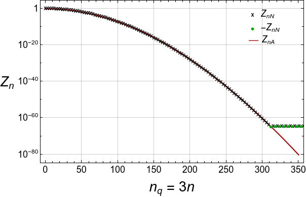
Figure 1: $Z_{nN}$ (blue crosses) are compared with $Z_{nA}$ (red line) for $N_{s}=16$. For $n_{q}>309$ positive values of $Z_{nN}$ are shown by crosses, whereas for negative $Z_{nN}$ we depict $-Z_{nN}$ using green circles.

To compare $Z_{nN}$ and $Z_{nA}$ more explicitly, we compute the relative deviation,

$$R=(Z_{nN}-Z_{nA})/Z_{nN},$$

for three volumes at $\varrho_{n}\leq 1.6$. We find that at $\varrho_{n}<1.5$, the relative deviation is rather small ($R<0.04$), but it increases rather fast, reaching 0.2 at $\varrho_{n}=\varrho_{n_{c}}$. We shall note that the numerical values for $a_{1}=4.671(14)$ and $a_{3}=0.992(25)$ were obtained on $N_{s}=16$ lattices, and we used the same values for all volumes assuming a very weak volume dependence of $a_{i}$. Our numerical results on volume dependence of $a_{i}$ Bornyakov:2016wld support this. Thus, by volume dependence, we will understand the dependence of various observables on $N_{s}$ through eq. (13). We checked that variation of $a_{i}$ within error bars given above did not alter any of our conclusions, although respective variation of $Z_{nA}$ for large $n$ was quite substantial.

In fact, the expression (15) is not the whole story. One can take into account the fluctuations around $\theta_{0}$ to obtain

$$Z_{nA}=\frac{e^{-\nu F_{n}(\theta_{0})}}{e^{-\nu F_{0}(\theta_{0})}}\frac{\sqrt{F_{0}^{\prime\prime}(\theta_{0})}}{\sqrt{F_{n}^{\prime\prime}(\theta_{0})}}$$ (16)

where

$$F_{n}^{\prime\prime}(\theta_{0})=a_{1}+3a_{3}\theta_{0}^{2}\;.$$ (17)

Eq. (16) corresponds to the next-to-leading approximation in the asymptotic expansion (13) consisting in taking into account the pre-exponential factor. In principle, higher-order approximations can also be taken into account. However, we leave this for future studies. We find that our result eq. (16) is much closer to $Z_{nN}$ than the result eq. (15) obtained in RobergeWeiss . In this case, $R$ goes to zero in the infinite volume limit for all density values $\varrho_{max}$ under consideration.

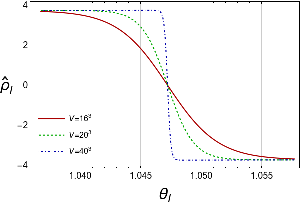
Figure 2: The quark number density computed using $Z_{nA}$ for imaginary chemical potential for three volumes and $\varrho_{max}=8.0$ over a restricted range near $\theta_{I}=\pi/3$.

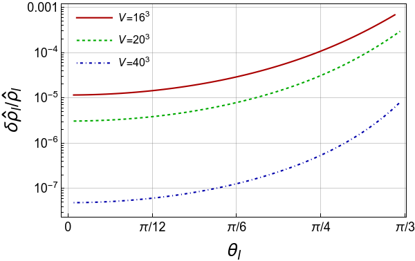
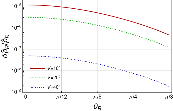
Figure 3: Relative deviation of the quark number density computed using $Z_{nA}$ for the imaginary chemical potential (left panel) and the real chemical potential (right panel).

Another way to check the quality of the obtained approximation for $Z_{n}$ is to compute the quark number density using the following relations: (see eqs. (5)-(6) in Bornyakov:2016wld ):

$$\hat{\rho}_{I} = {1\over\nu}\frac{2\sum_{n>0}nZ_{nA}\sin(n\theta_{I})}{1+2\sum_{n>0}Z_{nA}\cos(n\theta_{I})}\,,$$ (18)

$$\hat{\rho}_{R} = {1\over\nu}\frac{2\sum_{n>0}nZ_{nA}\sinh(n\theta_{R})}{1+2\sum_{n>0}Z_{nA}\cosh(n\theta_{R})}\,$$ (19)

and compare it with the input number density eq. (9) or with its analytical continuation to real values $\theta_{R}$. In Fig. 2 we show the quark number density $\hat{\rho}_{I}$ computed via $Z_{nA}$ in the vicinity of the critical value $\theta_{I}=\pi/3$. The volume dependence of the density becomes visible: with increasing volume, the number density approaches a step function, i.e. the first order phase transition appears in the infinite volume limit.

The relative deviations between results obtained for the quark number density via Eqs. (18), (19) and Eq. (9) are shown in Fig. 3 for three spatial volumes. In the left panel, it is shown for imaginary $\mu_{q}$. The deviation is small and shows a very fast decrease with increasing $V$. Note that the relative deviation increases near $\theta_{I}=\pi/3$ since for this range Eq. (9) gives a correct number density in the infinite volume limit only. In the right panel, we show the relative deviation for the real chemical potentials. Again we see that this relative deviation is small and decreases with volume increase. Moreover, one can see decreasing with increasing chemical potential.

For $a_{5}\neq 0$, an explicit solution of eq. (9) is not available. However, we find an approximate solution considering $a_{5}$ as a small parameter. Details of the computation are presented in Appendix. Since $a_{5}=0$ within error bars at $T=1.35T_{c}$ considered here, we estimated the corrections due to higher-order terms at lower temperature $T=1.2T_{c}$. We found a good qualitative agreement between $Z_{nN}$ and $Z_{nA}$ for $n<n_{c}=291$: the relative deviation $|R|<0.04$ for $n<200$ and it runs up to $0.4$ as $n$ increases up to 290.

However, we should comment on the limitations of the asymptotic approximation eq. (13). If $n>N_{tot}=2N_{f}N_{s}^{3}$, where $N_{tot}$ is the total number of quark modes on the lattice under consideration,then lattice regularization yields $Z_{n}=0$, whereas $Z_{nA}\neq 0\ \ \forall n\;$. Therefore, the range of validity of the approximation (10) is

$$\varrho_{n}<\!\!\!<\varrho_{tot}={N_{tot}\over VT^{3}}=2N_{f}N_{t}^{3}\;.$$ (20)

The values of $\varrho_{n}$ used in our study are well below the indicated limit.

III Evaluation of Lee-Yang Zeros

Lee-Yang zeros are zeros of the grand canonical partition function $Z_{GC}(\theta,T,V)$, considered a polynomial of the baryon fugacity $\xi_{B}$. In the finite volume $V$, $Z_{GC}(\theta,T,V)$ can be presented as

$$Z_{GC}(\theta,T,V)=\sum_{n=-N_{tot}}^{N_{tot}}Z_{C}(n,T,V)\xi_{B}^{n}=e^{-N_{tot}N_{c}\theta}\sum_{n=0}^{2N_{tot}}Z_{C}(n-N_{tot},T,V)\xi_{B}^{n}\;,$$ (21)

Computation of the high-degree polynomial zeros, Eq. (21), is challenging. In this work, we employ a very efficient package, MPSolve v.3.1.8 (Multiprecision Polynomial Solver) MPsolve1 ; MPsolve2 , which provides calculation of polynomial roots with arbitrary precision.

In eq. (21) we rewrote $Z_{GC}(\theta,T,V)$ as a polynomial of degree $2N_{tot}$ which roots represent the values of the LYZ in the complex $\xi_{B}$-plane. Coefficients $Z_{C}(n,T,V)$ are computed using Eq. (16) with the GNU MPFR Library for multiple-precision floating-point computations. We performed calculations using the MPFR library with accuracy from 1000 to 6000 digits. We found that 1000 digits are enough for the MPSolve package to calculate LYZ for a polynomial with a degree less than 20000. We also checked that to compute LYZ for polynomials of degrees larger than 60000, it is necessary to use $Z_{nA}$ calculated with an accuracy of more than 6000 digits.

To make a conclusion about the infinite-volume limit, we have to study the dependence of the LYZ on $N_{s}$ and on the number of terms used in the sum eq. (21), which we denote as $N_{max}$ in what follows. Analytical expression (16) for the coefficients of the polynomial in Eq. (21) together with the use of the MPSolve package, allow us to work with an arbitrary degree of the polynomial limited only by the computational cost of LYZ calculation and to improve our previous results Wakayama:2018wkc substantially for $T>T_{RW}$. Our main goal is to understand the properties of LYZ in the vicinity of the RW transition at $\theta_{I}=\pi/3$.

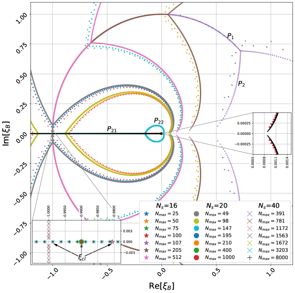
Figure 4: LYZ distribution in the fugacity plane. See explanation in the text.

In Fig. 4 the results for LYZ are presented in the fugacity plane for three volumes with $N_{s}=16,20,40$ and six values of $N_{max}$ for each volume. These values of $N_{max}$ change with volume and correspond to six volume independent values of the maximal quark number density $\varrho_{max}=N_{max}/(VT^{3})$. We start with $\varrho_{max}\approx 0.39$, and increase it up to $\varrho_{max}=8.0$. Note that below we discuss only LYZ located on and within the unit circle of the fugacity plane since the rest of LYZ can be restored using the property $Z_{GC}(\xi_{B})=Z_{GC}(1/\xi_{B})$.

It was found in Ref. Wakayama:2018wkc that the dependence on $\varrho_{max}$ is much more pronounced than the dependence on the volume. For small $\varrho_{max}$ LYZ consist of two parts (see Fig. 4): one part, $P_{1}$, comprises the LYZ distributed along the unit circle $|\xi_{B}|=1$ and the other, $P_{2}$, represents a curve starting on the circle at the end point of $P_{1}$ and extending towards the real positive axis. With increasing volume, the endpoint of $P_{2}$ tends to approach the real axis.

It was demonstrated in Wakayama:2018wkc that $P_{1}$ shrinks to $\xi_{B}=-1$ with increasing $\varrho_{max}$. Respectively, one end of $P_{2}$ moves along the unit circle towards $\xi_{B}=-1$ while the other end slowly moves in the direction of $\xi_{B}=0$. We now confirm these observations, as can be seen from the comparison of LYZ for $\varrho_{max}=0.39,0.78,1.17,1.56$ in Fig. 4. Moreover, while only the range $\varrho_{max}<1.6$ was studied in Ref. Wakayama:2018wkc due to the problem with computation of $Z_{n}$, here we present results for higher values $\varrho_{max}=1.67,3.20,8.0$. As a result, we discover the correct properties of the LYZ as described below.

In Fig. 4 one can see that $P_{1}$ disappears completely at $\varrho_{max}>\varrho_{n_{c}}\approx 1.6$. It is worth noting that this is approximately the same value of the quark density which is reachable in computations of $Z_{nN}$. It is natural to assume that the leading contributions to the grand canonical partition function come from all densities over the range $\varrho_{n}\leq\varrho_{n_{c}}$ and thus neglecting even part of them gives rise to unphysical results for the LYZ (the $P_{1}$ part on the unit circle).

It should be noticed that the first real negative LYZ also appears when $\varrho_{max}$ becomes as high as $\varrho_{n_{c}}$ for all volumes under consideration.

The $P_{2}$ line splits into two parts for $\varrho_{max}>\varrho_{n_{c}}$ $P_{21}$ and $P_{22}$. $P_{21}$ consists of LYZ on the segment $-1<\xi_{B}<-\xi_{B0}$ with $\xi_{B0}>0$ moving toward zero exponentially fast with increasing $\varrho_{max}$. The curly part $P_{22}$ connects $-\xi_{B0}$ with the point slightly above the positive real axis (see right insertion in Fig. 4). When we first increase $\varrho_{max}$ to its maximal value for a given volume (in practical terms, this implies the extrapolation to the infinite value) and then take the infinite volume limit, we expect that the right end of $P_{22}$ goes to $\xi_{B}=0$ and complex roots disappear completely. In fact, we found out that with increasing $\varrho_{max}$ the region occupied by the complex roots shrinks exponentially fast, but their share decreases rather slowly and remains finite. We believe that this difference between our expectations and real observation is due to artefacts of our approximation $Z_{nA}$.

Thus we see a very strong dependence of LYZ on $\varrho_{max}$. At the same time, as can be seen in Fig. 4 the finite volume effects are rather mild. For the maximal value of $\varrho_{max}$ shown in the figure, one can see these effects in the enlarged insertion only.

Next, we describe the properties of the LYZ on the real-negative axis. We found that for a fixed volume, they start to appear when $N_{max}$ exceeds some value roughly equal to $\displaystyle\varrho_{n_{c}}\cdot VT^{3}$. The LYZ most close to $\xi_{B}=-1$ appear first and, with increasing $N_{max}$, additional LYZ, more and more remoted from -1, also appear. This property of LYZ one can see in Fig. 4 ($P_{21}$ increases its length). In the left-bottom insertion in Fig. 4 the interval close to $\xi_{B}=-1$ is presented. It is seen that for fixed $N_{s}$ the position of the LYZ located on the real axes is not depending on $N_{max}$. In this insertion we also introduce the notation $\xi_{cl}$ as the location of the negative real LYZ closest to $\xi_{B}=-1$.

We approximate the normalized density of LYZ on the real axis, defined as

$$g(\theta_{R})={1\over N_{s}^{3}}\frac{dN_{LYZ}(\theta_{R})}{d\theta_{R}}\,,$$ (22)

where $N_{LYZ}(\theta_{R})$ is the number of LYZ in the interval between 0 and $\theta_{R}$, with

$$g(\theta_{R})=\frac{1}{N_{s}^{3}\;\Delta\theta_{R}}\,,$$ (23)

where $\Delta\theta_{R}$ is the distance between adjacent LYZ on the real negative semi-axis.

The formula relating the LYZ density to the discontinuity in the average particle-number density was obtained in Lee:1952ig . Analogously, for the quark number density $\hat{\rho}_{I}$, it is straightforward to show that its discontinuity $\Delta\hat{\rho}_{I}$ is related to the density of LYZ on the real axis as

$$\Delta\hat{\rho}_{I}=2\pi N_{c}N_{t}^{3}g(\theta_{R})\,.$$ (24)

It should be noted that this formula is exact only in the infinite-volume limit. Taking Eq. (9) continued to the complex plane one obtains for the discontinuity $\Delta\hat{\rho}_{I}$ at $\displaystyle\theta_{I}={\pi\over 3}$ the following dependence on $\theta_{R}$:

$$\Delta\hat{\rho}_{I}=2\Big{(}a_{1}\frac{\pi}{3}+a_{3}\frac{\pi^{3}}{27}-a_{3}\pi\theta_{R}^{2}\Big{)}$$ (25)

We show in the left panel of Fig. 5 both parts of eq. (24) as functions of $\theta_{R}$, results for the right hand side are presented for $N_{s}=16,20,40$. Dependence on $N_{S}$ is visible only in the vicinity of $\theta_{R}=0$. One can see that Eq. (24) is nicely satisfied (the relative deviation for $N_{s}=40$ is below 0.003) indicating once more that our approximation $Z_{nA}$ for the canonical partition functions works extremely well. Note that we show in this figure also the LYZ for positive $\theta_{R}$ corresponding to $|\xi_{B}|>1$. The symmetry seen in the figure demonstrates the property $Z_{GC}(\xi_{B})=Z_{GC}(1/\xi_{B})$ mentioned above.

Thus we conclude that in the infinite-volume limit, the density of LYZ does not vanish over the entire negative real semiaxis in the fugacity plane, including the point $\xi_{RW}=-1$. According to the criterion suggested in Lee:1952ig , the phase transition occurs at $Im(\mu_{B}/T)=\pi$. Yet another piece of evidence for our conclusion comes from $N_{s}$ dependence of the distance $|\xi_{RW}-\xi_{cl}|$, where $\xi_{cl}$ is the LYZ closest to $\xi_{RW}$. This dependence is shown in the right panel of Fig. 5, where results for $N_{s}=16,20,24,28,32,36,40$ are depicted. The constant $A$ of the fitting function provides an estimate of the LYZ density: $A=\frac{1}{2}g(0)$. Analogous results can be obtained for other values of $\xi$ on the negative real semi-axis.

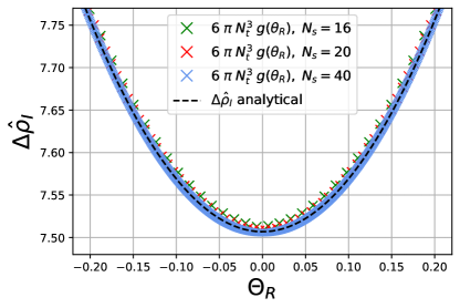
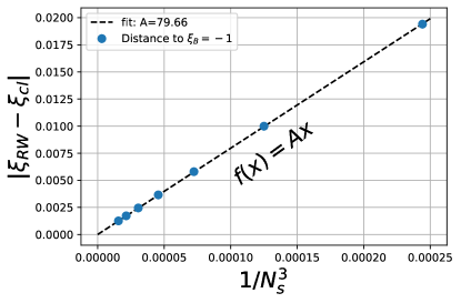
Figure 5: Left: lhs and rhs (for $N_{s}=16,20,40$) of eq. (24) vs. $\theta_{R}$ at $\displaystyle\theta_{I}=\pi/3$. Right: $N_{s}$ dependence of the distance between the point $\xi_{B}=-1$ and the nearest LYZ.

IV Conclusions

We have studied $N_{f}=2$ lattice QCD in the deconfinement phase above $T_{RW}$ at $T/T_{c}=1.35$. Our goal was to compute the distribution pattern of LYZ in the complex fugacity $\xi_{B}$ plane and to demonstrate the existence of the LYZ corresponding to the RW transition at imaginary quark chemical potential $\mu_{qI}/T=\pi/3$.

In our earlier work Wakayama:2018wkc we had performed computations of LYZ at $T>T_{RW}$ using a limited number of canonical partition functions $Z_{nN}$ computed numerically via the Fourier transform. We then found that $Z_{nN}$ could be computed only for a restricted range of $n$. To overcome this restriction, we have used the approximate analytical expression $Z_{nA}$ in this work. We demonstrated that $Z_{nA}$ agree very well with values of $Z_{nN}$ where the latter are available and reproduce the input expression for the quark number density. In both cases, the agreement improves with increasing volume. Using $Z_{nA}$, we have obtained the behavior for the quark number density in the vicinity of the RW phase transition at $\theta_{I}=\pi/3$ which is consistent with first principles. We shown that, in the infinite volume limit, there appears a discontinuity in the dependence of $\hat{\rho_{I}}$ on $\theta_{I}$ indicating the first-order transition behavior.

After we ensured that $Z_{nA}$ works very well, we computed the LYZ. Apart from increasing the available maximal density $\varrho_{max}$ which is now restricted only by the computation resources we also used a more effective procedure to compute LYZ, which employs the MPSolve library with arbitrary precision. Our computations have been performed with precision up to 6000 significant digits.

We confirmed our previous results about the strong dependence of LYZ on $\varrho_{max}$ and comparatively weak volume dependence, which were obtained in Wakayama:2018wkc with restricted $\varrho_{max}$.

Then, increasing $\varrho_{max}$, we have discovered that the LYZ appear on the $\xi$ negative real half-axis. In the infinite volume limit, LYZ tend to fill the full $Re(\xi)\leq 0$ range and have a non-vanishing density corresponding to the RW phase transition. We demonstrated that in the limit of high $\varrho_{max}$ LYZ exist away from the $\xi$ negative real axis, but only in the tiny vicinity of $\xi=0$ point. We believe that these LYZ are artefacts of our approximation $Z_{nA}$.

We derived the relation between the quark number density discontinuity $\Delta\rho_{I}$ and the LYZ density eq. (24) and observed that our numerical results for the LYZ density nicely satisfy this relation (see Fig. 5, left panel). This agreement demonstrates once more that approximation $Z_{nA}$ works extremely well.

Our result demonstrates the necessity of using sufficiently high values of $\varrho_{max}$ to obtain correct results for LYZ. We believe that our results, obtained at a high temperature where phase transitions are absent at real chemical potential, will be useful for the computation of LYZ at a low temperature where phase transition or crossover at real $\mu_{B}$ is present. This work is now underway.

Appendix A Corrections for $a_{5}\neq 0$.

The approximate solution $\theta$ of the equation

$$a_{5}\theta^{5}+a_{3}\theta^{3}+a_{1}\theta-\varrho_{n}=0$$ (26)

up to the order $a_{5}^{2}$ has the form

$$\theta=\theta_{0}+a_{5}\ \theta_{1}+a_{5}^{2}\ \theta_{2},$$ (27)

where $\theta_{0}$ is defined in eq. (14),

$$\theta_{1} = -\frac{\theta_{0}^{5}}{a_{1}+3a_{3}\theta_{0}^{2}}\;,$$ (28)

$$\theta_{2} = -\frac{5\theta_{1}\theta_{0}^{4}+3a_{3}\theta_{1}^{2}\theta_{0}}{a_{1}+3a_{3}\theta_{0}^{2}}\;.$$ (29)

Then we follow the procedure described in eqs. (10-16) and obtain

$$Z_{nA}=\frac{e^{-\nu F_{n}(\theta)}}{e^{-\nu F_{0}(\theta)}}\frac{\sqrt{F_{0}^{\prime\prime}(\theta)}}{\sqrt{F_{n}^{\prime\prime}(\theta)}}\,,$$ (30)

where

$$F_{n}(\theta)=-\frac{1}{4}(a_{1}\theta_{0}^{2}-3\varrho_{n}\theta_{0}+a_{5}f_{1}(\theta_{0})+a_{5}^{2}f_{2}(\theta_{0})+O(a_{5}^{3}))\,,$$ (31)

$$F_{n}^{\prime\prime}(\theta)=a_{1}+3a_{3}\theta_{0}^{2}+a_{5}f_{3}(\theta_{0})+a_{5}^{2}f_{4}(\theta_{0})+O(a_{5}^{3})$$ (32)

and

$$f_{1}(\theta_{0}) = \frac{2}{3}\theta_{0}^{6}\,,$$ (33a)

$$f_{2}(\theta_{0}) = -\frac{2\theta_{0}^{10}}{a_{1}+3a_{3}\theta_{0}^{2}}\,,$$ (33b)

$$f_{3}(\theta_{0}) = \theta_{0}^{4}\left(3+\frac{2a_{1}}{a_{1}+3a_{3}\theta_{0}^{2}}\right)\,,$$ (33c)

$$f_{4}(\theta_{0}) = -\theta_{0}^{8}\frac{20a_{1}^{2}+87a_{1}a_{3}\theta_{0}^{2}+99a_{3}^{2}\theta_{0}^{4}}{(a_{1}+3a_{3}\theta_{0}^{2})^{3}}\,.$$ (33d)

To compute $Z_{nA}$ for $T/T_{c}=1.20$ we use $a_{1}=4.409,a_{3}=1.032,a_{5}=-0.165$ Bornyakov:2016wld in eq. (9). It should be noted that with this set of constants $a_{i}$ eq. (9) is not applicable at large real chemical potential since the quark number density becomes negative at $\theta>3.028$. To keep the density positive we should assume that the coefficient $a_{7}$ which was not determined in Bornyakov:2016wld is positive.