MIGHTEE-$\textbf{H}\,\scriptstyle\mathbf{I}$: the $\textbf{H}\,\scriptstyle\mathbf{I}$ Size–Mass relation over the last billion years

Abstract

We present the observed H I size–mass relation of 204 galaxies from the MIGHTEE Survey Early Science data. The high sensitivity of MeerKAT allows us to detect galaxies spanning more than 4 orders of magnitude in H I mass, ranging from dwarf galaxies to massive spirals, and including all morphological types. This is the first time the relation has been explored on a blind homogeneous data set which extends over a previously unexplored redshift range of $0<z<0.084$, i.e. a period of around one billion years in cosmic time. The sample follows the same tight logarithmic relation derived from previous work, between the diameter ($D_{\mathrm{HI}}$) and the mass ($M_{\mathrm{HI}}$) of H I discs. We measure a slope of 0.501$\pm$ 0.008, an intercept of $-3.252^{+0.073}_{-0.074}$, and an observed scatter of 0.057 dex. For the first time, we quantify the intrinsic scatter of $0.054\pm 0.003$ dex (${\sim}10\%$), which provides a constraint for cosmological simulations of galaxy formation and evolution. We derive the relation as a function of galaxy type and find that their intrinsic scatters and slopes are consistent within the errors. We also calculate the $D_{\mathrm{HI}}$ – $M_{\mathrm{HI}}$ relation for two redshift bins and do not find any evidence for evolution with redshift. These results suggest that over a period of one billion years in lookback time, galaxy discs have not undergone significant evolution in their gas distribution and mean surface mass density, indicating a lack of dependence on both morphological type and redshift.

1 Introduction

Galaxies are gravitationally bound systems of stars, gas and dark matter. The processes governing their full gas cycle remain an area of active research. Theories of galaxy formation and evolution predict the gas infall onto galaxies to be the main mechanism supporting star formation and galaxy growth (Giovanelli & Haynes, 1988). Galaxies must continuously accrete gas from an external environment to maintain their observed levels of star formation (e.g. Kereš et al., 2005; Sancisi et al., 2008; Kauffmann et al., 2010). Consequently, the environment in which a galaxy resides affects its evolution and thus its stellar mass and morphology (see Baldry et al., 2006; Peng et al., 2010). Dense environments, for example, not only prevent further accretion of gas and ongoing star formation, but also play the crucial role in active gas stripping and subsequent loss of gas from galaxies. This can be observed through the morphology-density relation described in Dressler et al. (1997), where high-density environments are populated by early-type galaxies (E, S0) whereas low-density environments are more dominated by late-type galaxies (S, Irr).

In addition to the morphology-density relation, other relations that provide insights into galaxy evolution include the baryonic Tully-Fisher relation (baryonic mass vs. rotational velocity; e.g. McGaugh et al. 2000; Lelli et al. 2019; Ponomareva et al. 2018; Ponomareva et al. 2021); the relation between optical and H I diameters (Broeils & Rhee, 1997; Leroy et al., 2008); star formation histories, stellar masses and structural parameters (Kauffmann et al., 2003); and the mass-metallicity relation (Tremonti et al., 2004).

Another fundamental scaling relation for disc galaxies is the H I size-mass relation. First discovered by Broeils & Rhee (1997), it shows a tight correlation between the diameter of an H I disc ($D_{\mathrm{HI}}$), measured at a surface mass density level of 1 $\rm M_{\odot}\,pc^{-2}$, and its total enclosed H I mass ($M_{\mathrm{HI}}$). Recent studies have demonstrated that this relation also holds true over a wide range of galaxy types, such as large spirals (Verheijen & Sancisi, 2001; Swaters et al., 2002; Wang et al., 2013; Lelli et al., 2016; Ponomareva et al., 2016), late-type dwarf galaxies (Swaters et al., 2002; Begum et al., 2008; Lelli et al., 2016), early-type spirals (Noordermeer et al., 2005), irregulars (Lelli et al., 2016) and even for the ultra-diffuse galaxies (UDGs) discovered in the Arecibo Legacy Fast ALFA (ALFALFA) survey (Leisman et al., 2017; Gault et al., 2021). Moreover, even though the intergalactic medium (IGM) of groups and clusters can affect the sizes of H I discs due to ram-pressure and tidal interactions (Verdes-Montenegro et al., 2001), it was shown that galaxies which reside in groups and clusters still follow the observed H I size-mass relation as long as their discs are not too disrupted and the diameter can be traced out to 1 $\rm M_{\odot}\,pc^{-2}$ (Verheijen & Sancisi, 2001; Chung et al., 2009).

The galaxies in hydrodynamical simulations and semi-analytical models also follow the observed scaling relation between the H I mass and size, with an analytically derived limit on its scatter of $\leq 0.1~{}\rm dex$ (e.g. Wang et al. 2014; Marinacci et al. 2017; El-Badry et al. 2018; Lutz et al. 2018). Although, environmental processes such as ram-pressure stripping may cause galaxy discs to truncate or have holes, this does not strongly affect the relation unless the disc is completely disturbed (Stevens et al., 2019). Moreover, Stevens et al. (2019) have shown that the robustness of the H I size-mass relation makes it a valuable tool for theories of galaxy formation and evolution: the success of any model or simulation should be based on its ability to reproduce its scatter, slope and zero point with only a few percent uncertainty.

The largest observational work-to-date was undertaken by Wang et al. (2016), who collected H I sizes for more than 500 galaxies from 14 various projects, ranging over five decades in $M_{\mathrm{HI}}$. They obtained a remarkably tight relation with a scatter of 0.06 dex (14%). Although low-mass galaxies were found to have denser H I discs than higher-mass galaxies due to their low angular momentum (Lelli et al., 2016), the tight power law correlation indicates a nearly constant characteristic H I surface density within $D_{\mathrm{HI}}$ for most galaxies (Wang et al., 2016) – regardless of their type, mass, or environment. This relation therefore suggests that all galaxies, from small dwarfs to large spirals, experience a similar process of evolution as long as they remain gas-rich.

Little is known about the resolved H I content of galaxies located beyond the local Universe, mostly due to technical limitations such as lack of sensitivity and narrow frequency coverage of radio interferometers. To date, only a few surveys observed H I in galaxies at $z>0.01$ (e.g., the Blind Ultra-Deep H I Environmental Survey (BUDHIES; Gogate et al. 2020) and HIGHz; Catinella & Cortese 2015). The highest redshift H I detection until now is a starburst galaxy found in the COSMOS H I Large Extragalactic Survey (CHILES) at $z=0.376$ (Fernández et al., 2016). Therefore, the size-mass relation has only been studied for various nearby H I-selected samples, and remains unexplored for large, homogeneous samples, which extend to higher redshifts. With the advent of deep H I surveys with the Square Kilometre Array (SKA) pathfinders (and eventually the SKA itself), a new window is opening for studying the H I content of galaxies beyond the local volume.

This work is based on the Early Science data from the MeerKAT International GHz Tiered Extragalactic Exploration (MIGHTEE) survey (Jarvis et al., 2016). Our sample comprises 276 galaxies detected as part of the spectral line component of MIGHTEE. The sample spans more than four orders of magnitude in H I mass and one billion years in lookback time ($z\leq 0.084$). Therefore, we are able to study the H I size-mass relation for the first time beyond the local Universe using a homogeneous data set, and explore its possible evolution with redshift.

Our paper is structured as follows: we summarize the MeerKAT observations and data reduction strategy in Section 2. Sample selection and morphological galaxy classification are described in Section 3. In Sections 4 and 5, we present the measurements of the H I size and mass of our sample galaxies, respectively. We analyse our results and compare them with existing studies in Section 6. Section 7 summarizes our findings.

Throughout this paper, we assume $\Lambda$CDM cosmology parameters of $\Omega_{\rm m}=0.3$, $\Omega_{\Lambda}=0.7$ and $H_{0}=70$ kms${}^{-1}\,$ $\rm Mpc^{-1}$, for ease of comparison with previous results.

2 MEERKAT observations and data reduction

MIGHTEE is one of the eight Large Survey Project (LSP) of MeerKAT (Jonas & MeerKAT Team, 2016). MIGHTEE science cases include studies of the radio continuum (see Heywood et al. 2021 for the early science data release), H I in emission (MIGHTEE-H I), H I absorption and polarisation in galaxies. This study focuses on the MIGHTEE-H I part of the survey, and uses the Early Science data, details of which can be found in Maddox et al. (2021).

The observations were carried out with the full MeerKAT array between mid-2018 and mid-2019 in the L-band. The data were collected using the 4k spectral line correlator mode, with a channel width of 209 kHz, which corresponds to a velocity resolution of 44.11 kms${}^{-1}\,$ at $z=0$. The observations were carried out over two of four MIGHTEE fields described in Jarvis et al. (2016), covering approximately 3.5 deg² of the sky in XMMLSS and 1.5 deg² in COSMOS, resulting in a total area of ${\sim}5~{}\rm deg^{2}$.

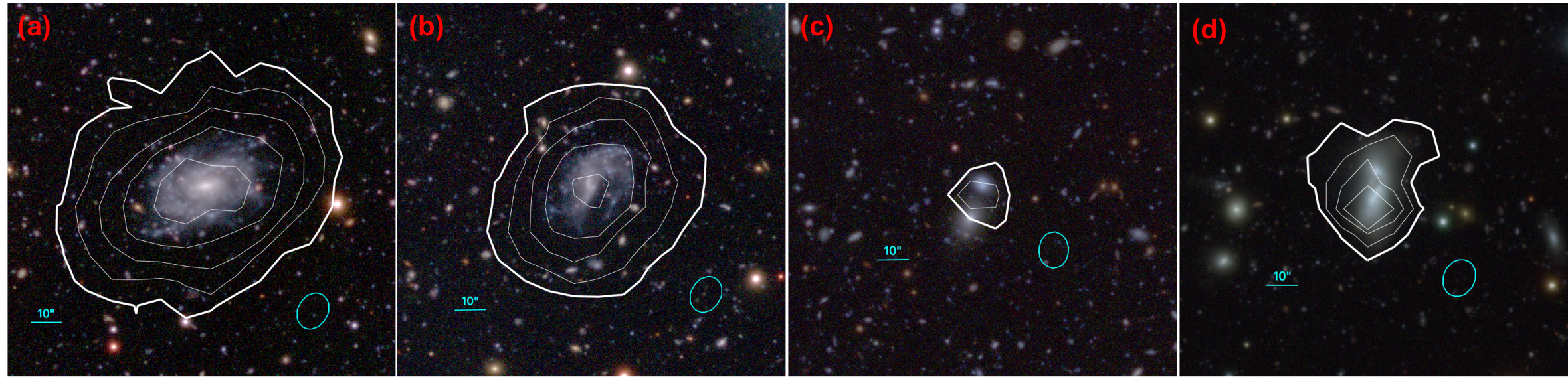
Figure 1: Examples of galaxies of different morphological types detected within MIGHTEE-H I. Panel (a): an undisturbed spiral galaxy at $z=0.033$; panel (b): an irregular galaxy at $z=0.044$; panel (c): an early-type galaxy (the northern counterpart) at $z=0.037$; panel (d): a merging system at $z=0.032$. The optical cutouts are from the HSC gri images, with the H I column density contours overlaid in white. The $1.25\times 10^{20}$ atoms cm^-2 (1 $\rm M_{\odot}\,pc^{-2}$) contour is shown in bold. Thin contours correspond to $3,6,10,15\times 10^{20}$ atoms cm^-2 for panels (a) and (b), $2\times 10^{20}$ atoms cm^-2 for panel (c), and $2,3,4\times 10^{20}$ atoms cm^-2 for panel (d). A 10″ scale bar and the synthesized beam size are displayed in each panel, in which panel (c) has a slightly different angle due to it being from a different field than the other panels.

Data calibration tasks such as flagging, delay, bandpass, gain and self-calibration were done with the ProcessMeerKAT pipeline Collier et al. (in preparation). This is a Casa-based pipeline developed at the Inter-University Institute for Data Intensive Astronomy (IDIA).

Visibility based continuum subtraction was done in two steps – an initial subtraction of the best clean component continuum model and the subtraction of a polynomial fit to the per-baseline/per-integration spectrum. The residual visibilities were imaged using Casa’s TCLEAN task with Briggs (1995) weighting (robust = 0.5). A final step of median-filtering was done on the cubes to reduce the impact of continuum-subtraction errors. Full details of the data processing can be found in Frank et al. (in prep).

The H I cube is ${\sim}2.3^{\circ}\times 2.3^{\circ}$ per pointing. The dirty beam FWHM’s are $$$\times$$$ and $$$\times$$$ for the COSMOS and XMMLSS fields, respectively. A 3$\sigma$ column density sensitivity in COSMOS is $4.05\times 10^{19}$ atoms cm^-2  and $9.83\times 10^{19}$ atoms cm^-2 in XMMLSS. The observational and imaging parameters of the Early Science data are summarized in Table 1.

Table 1: A summary of the MeerKAT observing parameters and imaging of the MIGHTEE-H I Early Science data.

Observing parameters	Value
Survey area	1.5 deg2 (COSMOS field)
	3 $\times$ 1.2 deg2 (XMMLSS field)
Total integration time	${\sim}17$ hrs (COSMOS)
	3 $\times$ 13 hrs (XMMLSS)
Spectral resolution	209 kHz
Velocity resolution	44.11 kms${}^{-1}\,$ at $z=0$
Velocity range	86 – 24205 kms${}^{-1}\,$
PSF (FWHM)	$$$\times$$$ (COSMOS)
	$$$\times$$$ (XMMLSS)
Pixel / Image size	$2\mathrm{″}$ / $4096\times 4096$
$3\sigma$ H I column density sensitivity	$4.05\times 10^{19}$ atoms cm-2 (COSMOS)
	$9.83\times 10^{19}$ atoms cm-2 (XMMLSS)

3 Sample selection

Source finding was performed visually on the Early Science data cubes covering 1310 – 1420 MHz, as described in Maddox et al. (2021). This resulted in 276 unique H I detections, forming the basis for our analysis. There were no restrictions on redshift, morphology, mass, or environment, i.e. all detections were initially considered for the current study.

After an in-depth examination of the sources, four galaxies were removed from the sample because they were classified as intermediate-stage mergers, i.e. when a system comprises two distinct stellar discs, but a single H I structure encompassing both galaxies. Early-stage mergers, where H I discs are still associated with the individual galaxies were kept in the sample. Late-stage mergers, where the H I and the stars have both merged into a single structure were also retained. After removing these four galaxies, our sample was reduced to 272 objects.

We further imposed that galaxies must be resolved with at least one and a half resolution elements across the major axis, and that the radial extent of the inclination corrected surface mass density ($\Sigma_{\rm HI}$, see Section 4) must reach 1 $\rm M_{\odot}\,pc^{-2}$ ($1.249\times 10^{20}\ \rm atoms\ cm^{-2}$). Even though the measurement of $D_{\rm HI}$ at 1 $\rm M_{\odot}\,pc^{-2}$ is a subjective choice, Wang et al. (2016) has shown that a diameter $D_{\rm HI}$ defined at 1 $\rm M_{\odot}\,pc^{-2}$ encloses most of the H I mass of a galaxy and is measurable for most of the galaxies, even for small H I discs that are close to being unresolved.

Additionally, the $\Sigma_{\rm HI}$ contour at 1 $\rm M_{\odot}\,pc^{-2}$ should not be strongly disrupted due to ongoing mergers or tidal interactions (for details, see Section 4). A total of 204 out of 272 galaxies satisfy our selection criteria, and form the final sample for our study of the $D_{\rm HI}$ – $M_{\rm HI}$ relation. The median resolution of our resulting sample is three beams across the major axis, with only 6 galaxies being resolved with more than 10 beams.

3.1 Morphological classification

The galaxies in our sample were visually classified based on their optical morphology. Three of the authors (SR, AP and NM) inspected three-colour images created from Subaru HyperSuprimeCam $g,r,$ and $i$-band images (HSC; Aihara et al. 2018, 2019). For the few (16 of 204) objects lying outside the HSC imaging footprint, the three-colour images from the Sloan Digital Sky Survey Data Release 16 (SDSS DR16; Ahumada et al. 2020) were used. The SDSS imaging is substantially shallower than that from HSC, but the number of objects is small, and the different imaging does not affect our results. The majority vote of the three classifiers was taken as the adopted morphology. While automated morphological classification algorithms are used for large datasets (e.g. the Zurich Estimator of Structural Type, Scarlata et al. 2007), visual classification is still in use (e.g. Hashemizadeh et al., 2021). The H I morphology was not used for the classification except to remove merging systems as noted before.

The galaxies were divided into four morphological categories: spirals (SP), early-types (ET), irregulars (IR) and mergers (ME). No distinction was made between irregulars and dwarf irregulars as no stellar mass information was used in the classification. ET galaxies have smooth, centrally concentrated morphology, whereas SP galaxies show clear spiral arms originating from either a central bulge or bulge/bar. IR objects show no regular patterns, and ME systems show signs of interaction between two or more galaxies, including disturbed morphology or tidal streams. Of the 204 galaxies in the original sample, there are 148 SP, 40 IR, 12 ME and 4 ET. Examples of the four classes are given in Fig. 1.

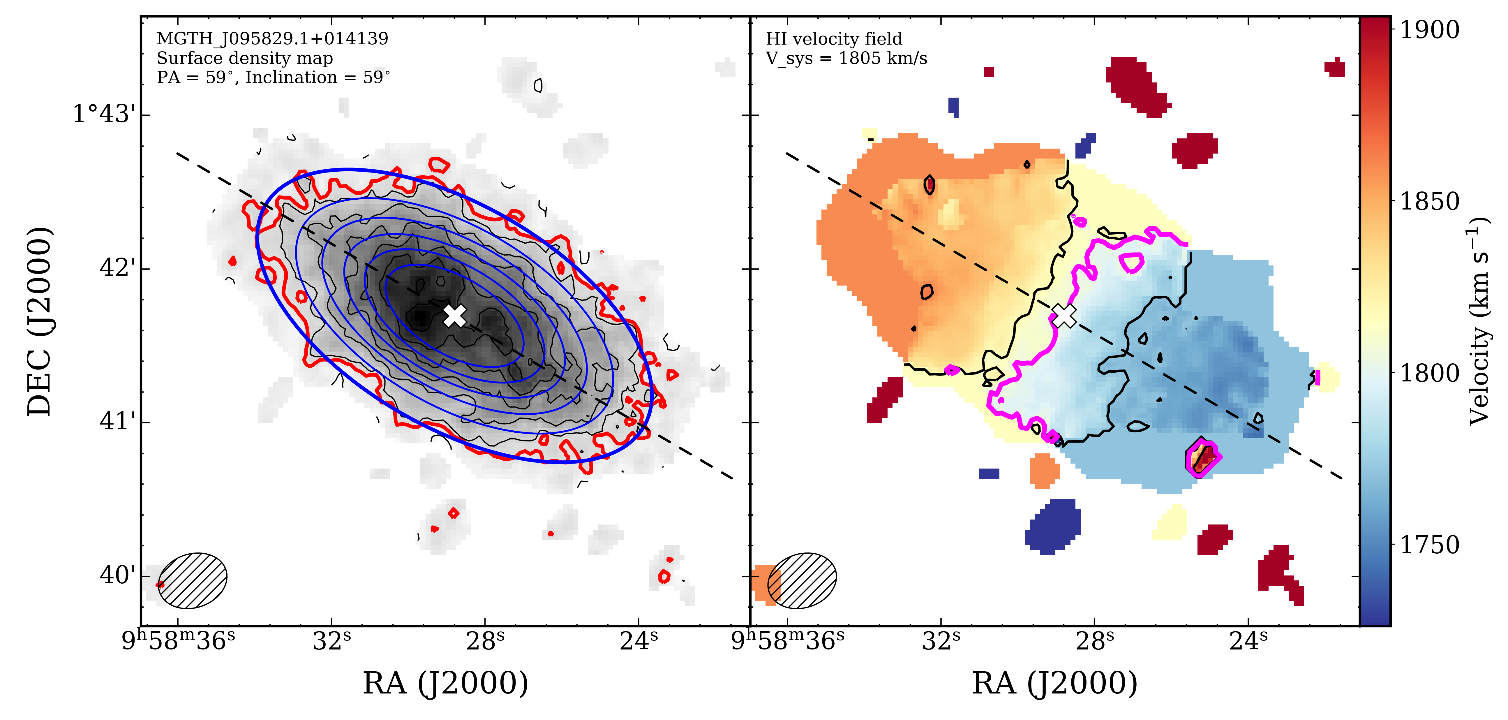
Figure 2: Example illustrating the 2D Gaussian fitting procedure (source MGTH_J095829.1+014139). Left panel: Surface mass density map (grey scale and black thin contours). The contour levels are 10.5, 9, 7.5, 6, 4.5, 3, 1.5 $\rm M_{\odot}\,pc^{-2}$ and the 1 $\rm M_{\odot}\,pc^{-2}$ contour is highlighted in red. The fitted 2D Gaussian function is shown by the thin blue ellipses; the fitted $D_{\rm HI}$ is highlighted by the thick blue outermost ellipse. Right panel: velocity field (moment 1). Iso-velocity contours are shown in black and separated by 45 kms${}^{-1}\,$. The measured systemic velocity is indicated by the thick magenta line. In both panels, the white cross marks the fitted ellipse centre, the dashed line represents the fitted major axis of the ellipse from the 2D Gaussian fitting. The beam size is indicated in the lower left corner of each panel.

4 $\textbf{H}\,\scriptstyle\mathbf{I}$ size

In order to measure the size of the H I discs, we use the moment 0 maps, produced for each detection as described in detail in Ponomareva et al. (2021) and Ranchod et al. (2021).

We convert moment 0 maps from the units of flux density to surface mass density following the prescription from Meyer et al. (2017):

$$\left(\frac{\Sigma_{\mathrm{HI}}}{\mathrm{M_{\odot}\,pc^{-2}}}\right)=1.00\times 10^{4}(1+z)^{3}\left(\frac{S}{\rm Jy\,km\,s^{-1}}\right)\left(\frac{\Omega_{\rm bm}}{\rm arcsec^{2}}\right)^{-1},$$ (1)

where $z$ is redshift, $S$ is flux density and $\Omega_{\rm bm}=\frac{\pi b_{\rm maj}b_{\rm min}}{4\rm ln(2)}$ is the solid angle of the synthesized beam with major axis $b_{\rm maj}$ and minor axis $b_{\rm min}$.

Once the surface mass density maps are obtained, we use the following approach to determine $D_{\rm HI}$:

1. We use a 2D elliptical Gaussian function to fit the surface mass density map and measure its diameter at the 1 $\rm M_{\odot}\,pc^{-2}$ contour level (see left panel of Fig. 2). It is important to note that the H I radial distribution is not Gaussian, and H I radial profiles often reveal a depletion at the center (e.g. Wang et al., 2014; Martinsson et al., 2016). However, we are only interested in H I distribution at the outer part of the H I disk where the H I diameter is measured. In addition, the majority of our sample galaxies are only marginally resolved with a median resolution of 3 beams. Therefore, a 2D elliptical Gaussian function works similar to a simple ellipse fitting. The function is expressed as:

   $$f(x,y)=A\exp{(-(a(x-x_{0})^{2}+2b(x-x_{0})(y-y_{0})+c(y-y_{0})^{2}))},$$ (2)

   where $A$ is the amplitude of the Gaussian peak in $\rm M_{\odot}\,pc^{-2}$, $(x_{0},y_{0})$ its centre position in pixels, and $a,b,$ and $c$ are defined as:

   $$a=\frac{\cos^{2}{\theta}}{2\sigma_{X}^{2}}+\frac{\sin^{2}{\theta}}{2\sigma_{Y}^{2}},$$ (3)

   $$b=-\frac{\sin{2\theta}}{4\sigma_{X}^{2}}+\frac{\sin{2\theta}}{4\sigma_{Y}^{2}},$$ (4)

   $$c=\frac{\sin^{2}{\theta}}{2\sigma_{X}^{2}}+\frac{\cos^{2}{\theta}}{2\sigma_{Y}^{2}}.$$ (5)

   In the above equations, $\theta$ is the position angle in radians, $\sigma_{X}$ and $\sigma_{Y}$ are the semi-major and semi-minor axes of the disk. We assume the following initial values for the parameters $A,x_{0},y_{0},\sigma_{X},\sigma_{Y}$ and $\theta$ to optimize the fitting process:

   • the amplitude $A$ is set to the maximum pixel value in the map in units of $\rm M_{\odot}\,pc^{-2}$,

   • the estimated H I emission centre $x_{0},y_{0}$ is assumed to be at the centre of the map i.e. half the number of pixels contained in the x and y axis of the map,

   • $\sigma_{X}$ and $\sigma_{Y}$ are set to 10 pixels as 20 pixels ($40\mathrm{″}$) is the typical extent of a source in the MIGHTEE-H I early science data,

   • the position angle $\theta$ was assumed to be 0.

2. With these estimates, we perform a non-linear least square fitting and obtain optimal values for the 2D Gaussian parameters listed in step (i). We use the 1 $\rm M_{\odot}\,pc^{-2}$ ellipse to obtain the corresponding best-fitting central position of the H I emission $(x_{0},y_{0})$, the major and minor axis values, and the position angle of the ellipse.

   As an example of the 2D Gaussian fitting, Fig. 2 displays the fitting outcome for a galaxy with $\rm V_{sys}\sim 1\,805~{}\rm km\,s^{-1}$ ($z=0.006$), where ellipses, resulted from the fit are over-plotted on top of the surface mass density map (left panel). The velocity field (right panel), though not being used in the fitting process, is shown to demonstrate that the fitted centre and major axis coincide with the kinematic centre and major axis.

   To derive the inclination angle of the plane of the galaxy in degrees, we use:

   $$\cos^{2}{(i_{\rm HI})}=\frac{(2.355\,\sigma_{Y})^{2}-b^{2}_{\rm min}}{(2.355\,\sigma_{X})^{2}-b^{2}_{\rm maj}},$$ (6)

   where $b_{\rm maj}$ and $b_{\rm min}$ are the major and minor axes of the synthesized beam (Verheijen & Sancisi, 2001). Galaxies with low spatial resolution might appear rounder due to the beam smearing. The inclusion of the synthesized beam in Eq. 6 will account for the beam smearing effect. However, it is important to note that this correction assumes that the axes of the beam are aligned with the axes of the galaxy, which is not necessary the case for our data. We ran the tests to evaluate the additional error on the inclination caused by possible misalignment of the beam and the source axes. We found that for marginally resolved galaxies ($<3$ beams) the error on inclination is ${\sim}7$ degrees, for galaxies resolved with 3 - 5 beams the error is ${\sim}3$ degrees, while it is negligible for galaxies resolved over more than 5 beams. We add these errors in quadrature to the inclination measurement error of ${\sim}5$ degrees (Ponomareva et al., 2021). This results in the total error on inclination for marginally resolved galaxies : ${\sim}8.5$ degrees, for galaxies resolved with 3 - 5 beams: 5.8 degrees, and 5 degrees for galaxies resolved with more than 5 beams. We also note that our inclinations, measured from the H I maps are in an excellent agreement with inclinations measured from the optical photometry and with inclinations derived with the 3D kinematic modelling for a sub-sample of 67 galaxies from Ponomareva et al. (2021).

3. We correct each surface mass density map for the measured inclination by multiplying each unmasked pixel value of the map by the cosine of the inclination angle. Then, we repeat steps (i) and (ii).

4. $D_{\rm HI}$ (2$\sigma_{X}$) is then measured from the inclination corrected maps along the major axis of the best-fitting ellipse corresponding to the surface mass density contour of 1 $\rm M_{\odot}\,pc^{-2}$.

5. To complete the H I size measurements, we correct $D_{\rm HI}$ for beam smearing effect using the following prescription from Wang et al. (2016):

   $$D_{\rm HI,corr}=\sqrt{D^{2}_{\rm HI}-b_{\rm maj}\times b_{\rm min}},$$ (7)

   where $D_{\rm HI,corr}$ is the corrected H I size which we use to construct the $D_{\rm HI}$ – $M_{\rm HI}$ relation. This correction removes a systematic bias which induces an over-estimation of $D_{\rm HI}$ for marginally resolved galaxies.

   The conservative uncertainty on $D_{\rm HI,corr}$ is assigned as half of the synthesized beam major axis $b_{\rm maj}$, expressed in kpc, and includes the uncertainty on the inclination angle. The error on the cosmological luminosity distance ($D_{L}$) is also propagated during the conversion. The latter was derived by adopting the channel width as the error on the systemic velocity and 2.2 $\rm km~{}s^{-1}~{}Mpc^{-1}$ as the error on the Hubble constant (Hinshaw et al., 2013). The resulting error on $D_{L}$ is ${\sim}3.5$ Mpc. The uncertainty on $\log D_{\rm HI}$ slightly increases with distance and is ${\sim}$0.02 kpc at $z=0$ and ${\sim}$0.11 kpc at $z\simeq 0.084$.

5 $\textbf{H}\,\scriptstyle\mathbf{I}$ mass

To construct the $D_{\rm HI}$ – $M_{\rm HI}$ relation, we measure the total H I mass enclosed within the moment 0 map of a galaxy, since the amount of H I beyond the diameter at 1 $\rm M_{\odot}\,pc^{-2}$ is negligible for our sample. By assuming an optically thin gas ($\tau\ll 1$) with no significant self-absorption, we use the following equation from Meyer et al. (2017) which uses the cosmological luminosity distance $D_{L}$ to the galaxy to determine the H I mass:

$$\left(\frac{M_{\rm HI}}{M_{\odot}}\right)\simeq\frac{2.356\times 10^{5}}{(1+z)}\left(\frac{D_{L}}{\rm Mpc}\right)^{2}\left(\frac{S}{\rm Jy\,km\,s^{-1}}\right),$$ (8)

where $z$ is the redshift, and $S=\int S_{v}dv$ is the integrated flux density derived from the moment 0 map.

The uncertainty on the integrated flux $S$ was estimated from the mean RMS noise within four emission-free regions around the detection (Ramatsoku et al., 2016; Ponomareva et al., 2021). As a result, an H I mass uncertainty of ${\sim}5\%$ is measured for large mass galaxies ($M_{\rm HI}>10^{9}~{}\rm M_{\odot}$), ${\sim}10\%$ for $10^{8}<M_{\rm HI}<10^{9}~{}\rm M_{\odot}$ while the error can reach up to 20% for galaxies below $M_{\rm HI}<10^{8}~{}\rm M_{\odot}$ (see Maddox et al. 2021 for details).

6 Results

This section presents the correlation between the H I mass and the H I size of the sample of 204 galaxies. We also show the comparison between the resulting $D_{\rm HI}$ – $M_{\rm HI}$ relation and previous studies at $z=0$, as well as its evolution as a function of redshift.

6.1 $D_{\mathrm{HI}}$ – $M_{\mathrm{HI}}$ relation

We construct the $D_{\mathrm{HI}}$ – $M_{\mathrm{HI}}$ relation and study its statistical properties, such as slope, zero point and scatter, by performing a power-law fit to the relation with a maximum likelihood function that takes measurement errors of both parameters into account, and assumes a Gaussian intrinsic scatter along the vertical direction to the best-fitting line (see Eq. A4 in Lelli et al. 2019). We can therefore investigate for the first time whether the previously reported small scatter of the relation ($\sigma=0.06$ dex, Wang et al. 2016) is due to measurement errors or is an intrinsic property.

We use the standard affine-invariant ensemble sampler for Markov chain Monte Carlo (MCMC) emcee (Foreman-Mackey et al., 2013) to map the posterior distributions of the main statistical properties: slope, zero point and intrinsic scatter of the relation, following the prescriptions described in Lelli et al. (2019).

For the fit, we initialize the chains with 50 random walkers, run 1000 iterations and re-run the simulation with 1000 steps. The starting position of the walkers is set randomly within realistic prior ranges: slope [0.1, 1], zero point [-6, 0] and intrinsic vertical scatter ($\sigma_{\text{int}}$) [0.01, 0.1]. The convergence of the chains is then checked visually.

The posterior distributions of the parameters are shown in Fig. 3 and their median values are listed in Table 2.

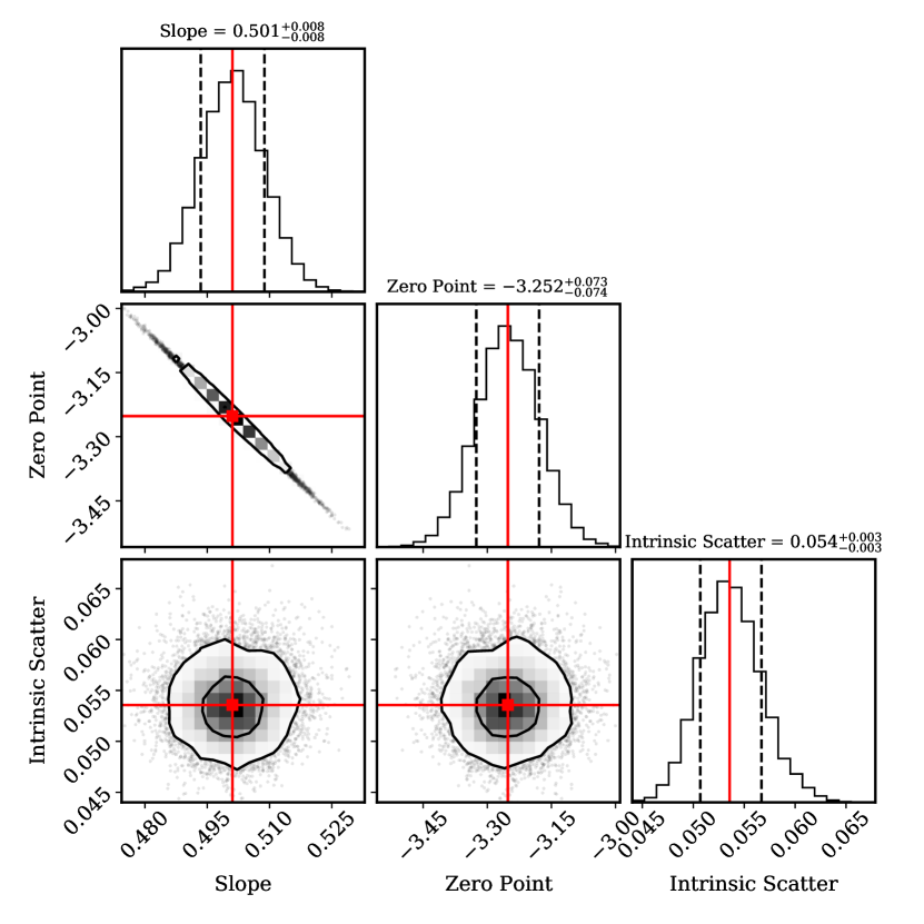
Figure 3: The posterior distributions of the slope, zero point and the intrinsic scatter of the $D_{\rm HI}$ – $M_{\rm HI}$. The best-fitting median values are indicated with the red squares and solid lines. Black contours are 68 ($1\sigma$) and 95 ($2\sigma$) per cent confidence regions.

The resulting $D_{\rm HI}$ – $M_{\rm HI}$ relation for our data and the associated 1$\sigma$ uncertainty from the MCMC posterior distribution is presented in Fig. 4. We find the relation to be:

$$\log D_{\rm HI}=0.501^{+0.008}_{-0.008}~{}\log M_{\rm HI}-3.252^{+0.073}_{-0.074}.$$ (9)

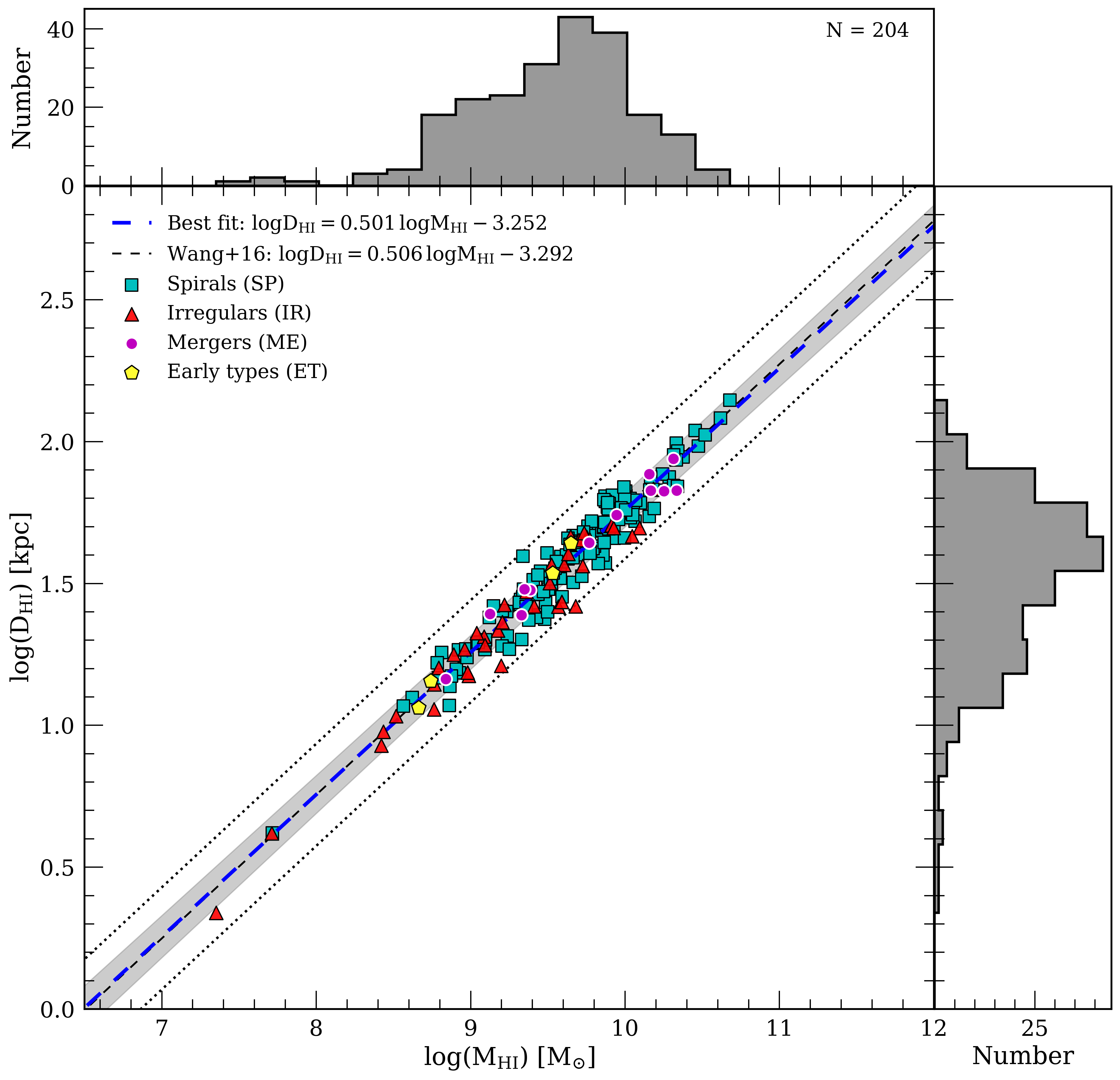
Figure 4: $D_{\mathrm{HI}}$ – $M_{\mathrm{HI}}$ relation for 204 inclination-corrected galaxies. Each symbol corresponds to one of the four morphological classifications: 148 spiral galaxies (SP: cyan squares), 40 irregular galaxies (IR: red triangles), 4 early-type galaxies (ET: yellow pentagons), and 12 merging systems (ME: magenta circles). The best-fitting relation is shown with the thick dashed blue line, while the best fit from Wang et al. (2016) is shown with a dotted black line. The shaded region indicates the $1\sigma$ uncertainty from the MCMC posteriors (see Fig. 3) and the black dotted lines delimit the $3\sigma$ scatter from Wang et al. (2016) relation. The histograms on the sides display the H I mass and H I size distributions of the galaxies in the sample, respectively.

The non-zero intrinsic scatter ($\sigma_{int}=0.054\pm 0.003$ dex) is comparable to the observed scatter ($\sigma=$ 0.057 dex) and suggests that the scatter of the relation cannot be explained just with the measurement errors, but rather is an intrinsic property of the relation allowing for a ${\sim}10\%$ variation of the $D_{\rm HI}$ at a fixed H I mass. To assess whether the intrinsic scatter is introduced by an underestimation of the measurement errors, we have repeated the fit using measurement errors which are 2, 3, and 4 times larger than the original values in both directions. Consequently, all resulting intrinsic scatters were non-zero.

Furthermore, our relation is in excellent agreement with Wang et al. (2016), who found a slope of $0.506\pm 0.003$, an intercept $-3.293\pm 0.009$, and an observed scatter of $\sigma=0.06$ dex.

Fig. 4 shows the distribution of the detections in the relation with respect to the $1\sigma$ confidence region of the MCMC fit and the $3\sigma$ scatter of the Wang et al. (2016) relation. It is observed that all detections lie within the black dotted lines which are the $3\sigma$ scatter of the Wang et al. (2016) relation.

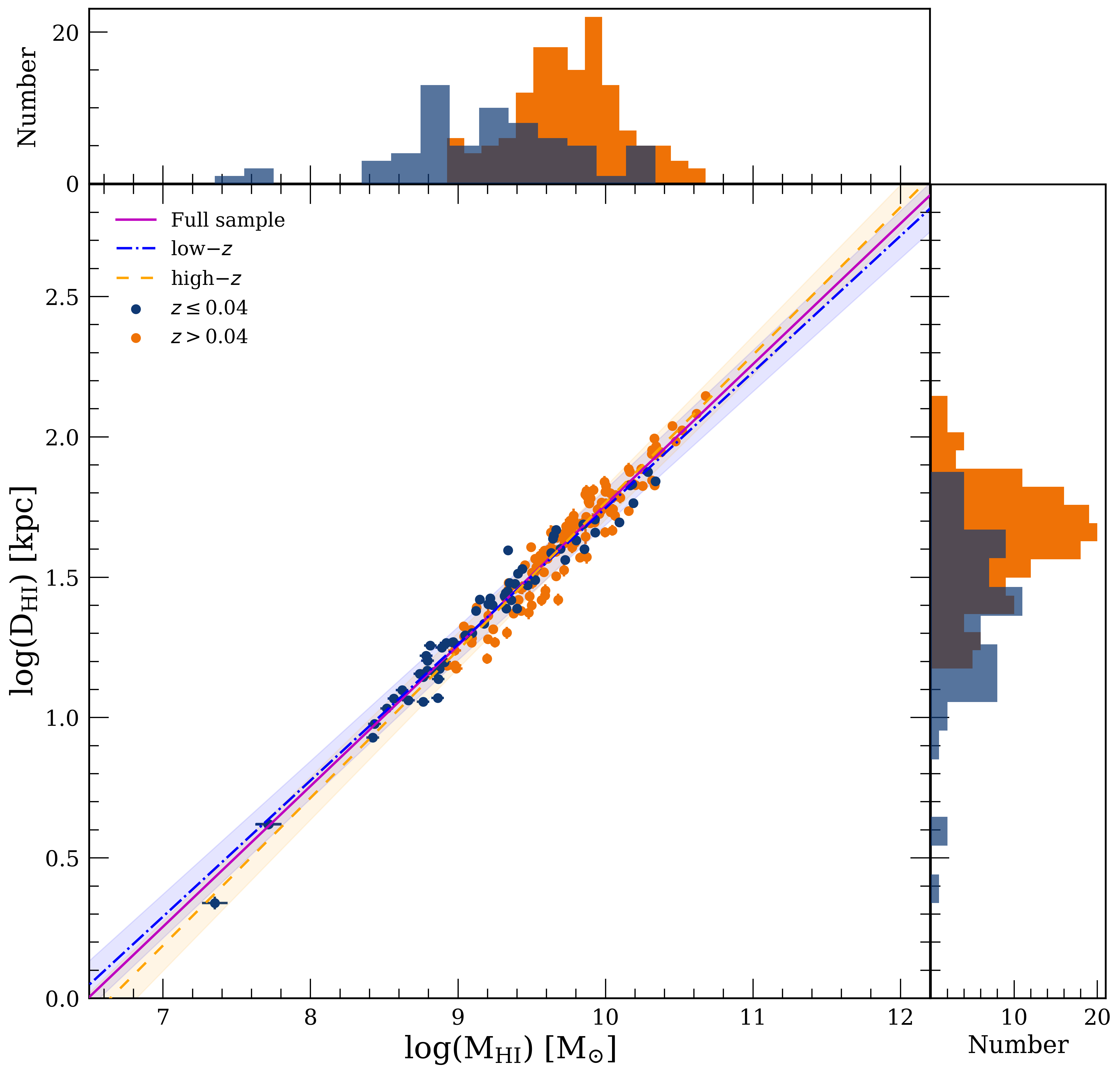
Figure 5: $D_{\rm HI}$ – $M_{\rm HI}$ relation of galaxies in the MIGHTEE-H I survey for two redshift bins. The errorbars on the points are approximately the same size as the points themselves. The high-redshift subsample ($z>0.04$) is presented in orange circles, the low-redshift subsample ($z\leq 0.04$) in blue. The magenta solid line indicates the best fit from the maximum-likelihood method of the full sample, while the orange dashed and the blue dashed-dotted lines represent the best fits from the high-redshit and the low-redshift subsamples respectively. Their respective 1$\sigma$ scatter is indicated by the shaded orange and blue regions. The H I mass and H I size distributions for the two redshift bins are displayed on the upper and right sides of the main frame.

6.2 $D_{\rm HI}$ – $M_{\rm HI}$ relation and galaxy type

Previous studies have focused on targeted morphologies of galaxies (e.g. Begum et al. 2008 with dwarf galaxies, Noordermeer et al. 2005 with early-type galaxies). The absence of a homogeneous large sample containing various types of galaxies has led to the study of the relation from compilations of data from various surveys (Lelli et al., 2016; Wang et al., 2016). This work is based on a “blind” survey, and as such, is not morphologically selected. To obtain further insight into the $D_{\rm HI}$ – $M_{\rm HI}$ relation, we explore the morphological properties of our sources, as classified in Section 3.1. The dominant morphological type in our sample is very similar to Wang et al. (2016) (SP and IR, with a few ET). Fig. 4 shows the $D_{\rm HI}$ – $M_{\rm HI}$ for our sample galaxies, grouped by morphological type, revealing that each subset of morphological types all lie on the relation and exhibits a low intrinsic scatter. The majority of SP/IR lie within the $1-2\sigma$ confidence region of the relation. It is important to note that our sample is H I-selected, and thus is sensitive towards relatively H I-rich galaxies. This is in contrast to the H I survey of early-type galaxies ATLAS^3D (Serra et al., 2012) which detected H I-poor ET galaxies below our column density limit and found that the typical H I column density of ETs is lower than of spiral galaxies (see Fig. 10 in Serra et al. 2012). Consequently, as far as ETs are concerned in this relation, we could not detect the faintest and H I-poorest ones due to a selection effect.

Table 2: Median values of the posterior distributions of the MCMC-based linear fit. Median H I mass and H I sizes for the $D_{\rm HI}$ – $M_{\rm HI}$ relation at different redshift bins, and the corresponding $\log D_{\rm HI}$ for a fixed $\log M_{\rm HI}$.

	$0\leq z\leq 0.084$	$z\leq 0.04$	$z>0.04$
Sample	N = 204	N = 63	N = 141
Slope	$0.501^{+0.008}_{-0.008}$	$0.485^{+0.012}_{-0.011}$	$0.526^{+0.013}_{-0.013}$
Intercept	$-3.252^{+0.073}_{-0.074}$	$-3.104^{+0.105}_{-0.107}$	$-3.494^{+0.125}_{-0.128}$
Scatter ($\sigma$)	0.057	0.054	0.058
Intrinsic scatter ($\sigma_{\rm int}$)	$0.054^{+0.003}_{-0.003}$	$0.052^{+0.006}_{-0.005}$	$0.053^{+0.004}_{-0.004}$
Median $\log(M_{\rm HI}[\rm M_{\odot}])$	9.64	9.22	9.75
Median $\log(D_{\rm HI}[\rm kpc])$	1.59	1.40	1.65
$\log D_{\rm HI}$	$1.579^{+0.015}_{-0.017}$	$1.573^{+0.021}_{-0.028}$	$1.579^{+0.029}_{-0.024}$
(at $\log M_{\rm HI}=9.64\,\rm M_{\odot}$)

We assess the intrinsic scatter and slope of the relation as a function of morphology. The 148 spiral galaxies show a tight intrinsic scatter of $0.053^{+0.004}_{-0.003}$ with a slope of $0.491\pm 0.010$, representing galaxies with large and well-defined discs. For the 40 irregulars, we find an intrinsic scatter of $0.061^{+0.009}_{-0.007}$ and a slope of $0.492^{+0.017}_{-0.016}$. This result indicates that the slopes of the $D_{\rm HI}$ – $M_{\rm HI}$ relations for SP and IR are statistically similar, and their intrinsic scatters are consistent within 2$\sigma$ error.

As highlighted in Section 3, only early and late-stage mergers, where the H I disc belongs to a single galaxy, were included in the ME sample. This would explain why the MEs in our sample lie on the relation. Due to the small sample sizes, we could not investigate the intrinsic scatter of MEs and ETs separately.

6.3 $D_{\rm HI}$ – $M_{\rm HI}$ relation and environment

The H I content of galaxies is known to be sensitive to the environment (Haynes et al., 1984). Verdes-Montenegro et al. (2001) have shown that the sizes of the H I discs of galaxies in group environments are influenced by tidal interactions. Continuous tidal stripping due to the IGM in groups can lead to the perturbed H I discs and H I deficiencies in galaxies. This was also investigated for simulated galaxies by Stevens et al. (2019), who showed that environmental processes, such as ram-pressure stripping, may cause disc truncation.

As mentioned in Section 3, we did not impose any environment-based constraint on our sample. There are indeed a variety of large-scale structures detected within the Early Science volume – the most prominent of which is the large galaxy group at $z\sim 0.044$, recently presented by Ranchod et al. (2021). This galaxy group consists of 20 galaxies distributed in a ${\sim}1\,\rm deg^{2}$ region and are all within a structure ${\sim}$400 kms${}^{-1}\,$wide. Its unusually high gas richness and non-Gaussian velocity dispersion distribution suggests a dynamically young group, still in its early stages of assembly. Mostly dominated by disk galaxies and few irregulars, it is an intermediate mass group, with dynamical mass of $\log_{10}(M_{\rm dyn}/\rm M_{\odot})=12.32$. We identified all galaxies within that overdensity, and found that all lie along the relation, suggesting that this group environment has not significantly affected the H I content of these galaxies. We measured a slope of $0.515\pm 0.019$ and an intercept of $-3.393^{+0.184}_{-0.185}$ for the structure, which is still consistent with the full sample. A more complete insight of the variation of the $D_{\rm HI}$ – $M_{\rm HI}$ relation with large scale environments will be achieved with the full MIGHTEE-H I survey area and redshift range.

6.4 Evolution of the $D_{\rm HI}$ – $M_{\rm HI}$ relation as a function of $z$

Whereas previous studies were restricted to the very nearby Universe, our sample and the relation derived from it extends over a previously unexplored redshift range. To investigate the evolution of the $D_{\rm HI}$ – $M_{\rm HI}$ as a function of redshift, we use our sample to test for any redshift dependence using similar approach as in Ponomareva et al. (2021). We divided our sample into two redshift bins with $z\leq 0.04$ and $z>0.04$, and performed the linear fit as described in Section 6.1 to each bin. The low-redshift subsample consists of 63 galaxies and spans four decades in H I mass ranging from $7.4\leq\log(M_{\rm HI}[\rm M_{\odot}])\leq 10.4$, with a median mass of $1.65\times 10^{9}\,\rm M_{\odot}$. The high-redshift subsample contains 141 galaxies covering 3 orders of magnitude in mass ($8.9\leq\log(M_{\rm HI}[\rm M_{\odot}])\leq 10.7$) and a median H I mass of $5.65\times 10^{9}\,\rm M_{\odot}$. Fig. 5 shows the best-fitting relation for each redshift bin. We observe marginal difference between the slope and intercept of the two subsamples, but the findings are consistent within the errors with the best-fitting relation of the full sample. The low-redshift bin has an intrinsic scatter of $0.052^{+0.006}_{-0.005}$ and observed scatter of 0.054 dex, which is consistent with Wang et al. (2016), whose sample only reaches out to redshifts of $z\sim 0.03$. The high-redshift bin has a slightly larger scatter, both intrinsic ($\sigma_{\rm int}=0.053^{+0.004}_{-0.003}$) and observed ($\sigma=0.058$), but is consistent within the errors (see Table 2).

To investigate the effect of a possible mass bias, we performed the fit once again for each subsample, for a common H I mass range of $8.9\leq\log(M_{\rm HI}[\rm M_{\odot}])\leq 10.4$. We observe a similar trend in the values of intrinsic scatter, slope, and only marginal difference is present between the low and high-$z$ subsamples with the fits being consistent within the errors. This supports the conclusion that the relation features no obvious evolution with redshift, which is consistent with predictions from hydrodynamical cosmological simulations of galaxy formation and evolution, e.g. NEWHORIZON (Dubois et al., 2021). However, this cannot be fully explored due to the still considerably small redshift range of our sample and will be further investigated with the full MIGHTEE-H I survey.

7 Summary and Conclusions

We have presented the $D_{\mathrm{HI}}$ – $M_{\mathrm{HI}}$ relation and measured the statistical properties of the homogeneous MIGHTEE-H I Early Science data sample which contains 204 galaxies, spans 4 decades in H I mass and extends to a redshift of $z\sim 0.084$.

We measured galaxy H I masses and used a novel 2D Gaussian fitting method to obtain the size of galaxy H I discs. We have also classified the galaxies based on their optical morphology. The main results of our study are as follows:

• For the first time, we are able to measure the intrinsic scatter of the $D_{\rm HI}$ – $M_{\rm HI}$ relation and find that it is non-zero. Therefore, we conclude that the relation allows for an intrinsic variation of ${\sim}10\%$ in $D_{\rm HI}$ at a given $M_{\rm HI}$.

• All of the galaxies in our sample are found to lie on the $D_{\rm HI}$ – $M_{\rm HI}$ relation, independent of morphological type. We also do not find any strong evidence for the environmental dependence when restricting our sample to the large group at $z\sim 0.044$.

• For the first time, we studied the $D_{\rm HI}$ – $M_{\rm HI}$ relation beyond $z>0.03$. We find no evidence that the relation has evolved over the last one billion years similarly to the baryonic Tully-Fisher relation (Ponomareva et al., 2021), suggesting that the galaxy discs have not undergone significant changes in their gas distribution and mean surface mass density over this period of time. This result is consistent with simulations of galaxy formation and evolution. For example, the latest results from the NEWHORIZON simulations show little-to-zero evolution over a Hubble time (Dubois et al., 2021).

• The measured statistical properties of the relation (slope, observed scatter and zero point) are entirely consistent with the largest $z=0$ study by Wang et al. (2016).
  

In conclusion, the successful study of the $D_{\rm HI}$ – $M_{\rm HI}$ relation using Early Science data from the MIGHTEE survey already substantiates MeerKAT’s potential for transformational H I science. The full MIGHTEE survey, covering 20 square degrees, will increase the explored volume out to $z\sim 0.5$, and will be crucial to study the evolution of the $D_{\rm HI}$ – $M_{\rm HI}$ relation as a function of redshift and large scale environments i.e. field vs groups, filaments and overdensities.

Data Availability

The MIGHTEE-H I spectral cubes will be released as part of the first data release of the MIGHTEE survey, which will include maps of the sources discussed in this paper. The data release is described in Frank et al. in prep. Data products used in this work are available upon reasonable request to the corresponding author.

References

- Ahumada et al. (2020) Ahumada R., et al., 2020, ApJS, 249, 3
- Aihara et al. (2018) Aihara H., et al., 2018, PASJ, 70, S4
- Aihara et al. (2019) Aihara H., et al., 2019, PASJ, 71, 114
- Astropy Collaboration et al. (2013) Astropy Collaboration et al., 2013, A&A, 558, A33
- Astropy Collaboration et al. (2018) Astropy Collaboration et al., 2018, AJ, 156, 123
- Baldry et al. (2006) Baldry I. K., Balogh M. L., Bower R. G., Glazebrook K., Nichol R. C., Bamford S. P., Budavari T., 2006, MNRAS, 373, 469
- Begum et al. (2008) Begum A., Chengalur J. N., Karachentsev I. D., Sharina M. E., Kaisin S. S., 2008, MNRAS, 386, 1667
- Briggs (1995) Briggs D. S., 1995, in American Astronomical Society Meeting Abstracts. p. 112.02
- Broeils & Rhee (1997) Broeils A. H., Rhee M. H., 1997, A&A, 324, 877
- Catinella & Cortese (2015) Catinella B., Cortese L., 2015, MNRAS, 446, 3526
- Chung et al. (2009) Chung A., van Gorkom J. H., Kenney J. D. P., Crowl H., Vollmer B., 2009, AJ, 138, 1741
- Dressler et al. (1997) Dressler A., et al., 1997, ApJ, 490, 577
- Dubois et al. (2021) Dubois Y., et al., 2021, A&A, 651, A109
- El-Badry et al. (2018) El-Badry K., et al., 2018, MNRAS, 473, 1930
- Fernández et al. (2016) Fernández X., et al., 2016, ApJ, 824, L1
- Foreman-Mackey et al. (2013) Foreman-Mackey D., Hogg D. W., Lang D., Goodman J., 2013, PASP, 125, 306
- Gault et al. (2021) Gault L., et al., 2021, ApJ, 909, 19
- Giovanelli & Haynes (1988) Giovanelli R., Haynes M. P., 1988, Extragalactic neutral hydrogen.. pp 522–562
- Gogate et al. (2020) Gogate A. R., Verheijen M. A. W., Deshev B. Z., van Gorkom J. H., Montero-Castaño M., van der Hulst J. M., Jaffé Y. L., Poggianti B. M., 2020, MNRAS, 496, 3531
- Hashemizadeh et al. (2021) Hashemizadeh A., et al., 2021, MNRAS, 505, 136
- Haynes et al. (1984) Haynes M. P., Giovanelli R., Chincarini G. L., 1984, ARA&A, 22, 445
- Heywood et al. (2021) Heywood I., et al., 2021, MNRAS,
- Hinshaw et al. (2013) Hinshaw G., et al., 2013, ApJS, 208, 19
- Jarvis et al. (2016) Jarvis M., et al., 2016, in MeerKAT Science: On the Pathway to the SKA. p. 6 (arXiv:1709.01901)
- Jonas & MeerKAT Team (2016) Jonas J., MeerKAT Team 2016, in MeerKAT Science: On the Pathway to the SKA. p. 1
- Kauffmann et al. (2003) Kauffmann G., et al., 2003, MNRAS, 341, 54
- Kauffmann et al. (2010) Kauffmann G., Li C., Heckman T. M., 2010, MNRAS, 409, 491
- Kereš et al. (2005) Kereš D., Katz N., Weinberg D. H., Davé R., 2005, MNRAS, 363, 2
- Leisman et al. (2017) Leisman L., et al., 2017, ApJ, 842, 133
- Lelli et al. (2016) Lelli F., McGaugh S. S., Schombert J. M., 2016, AJ, 152, 157
- Lelli et al. (2019) Lelli F., McGaugh S. S., Schombert J. M., Desmond H., Katz H., 2019, MNRAS, 484, 3267
- Leroy et al. (2008) Leroy A. K., Walter F., Brinks E., Bigiel F., de Blok W. J. G., Madore B., Thornley M. D., 2008, AJ, 136, 2782
- Lutz et al. (2018) Lutz K. A., et al., 2018, MNRAS, 476, 3744
- Maddox et al. (2021) Maddox N., et al., 2021, A&A, 646, A35
- Marinacci et al. (2017) Marinacci F., Grand R. J. J., Pakmor R., Springel V., Gómez F. A., Frenk C. S., White S. D. M., 2017, MNRAS, 466, 3859
- Martinsson et al. (2016) Martinsson T. P. K., Verheijen M. A. W., Bershady M. A., Westfall K. B., Andersen D. R., Swaters R. A., 2016, A&A, 585, A99
- McGaugh et al. (2000) McGaugh S. S., Schombert J. M., Bothun G. D., de Blok W. J. G., 2000, ApJ, 533, L99
- Meyer et al. (2017) Meyer M., Robotham A., Obreschkow D., Westmeier T., Duffy A. R., Staveley-Smith L., 2017, Publ. Astron. Soc. Australia, 34, 52
- Noordermeer et al. (2005) Noordermeer E., van der Hulst J. M., Sancisi R., Swaters R. A., van Albada T. S., 2005, A&A, 442, 137
- Peng et al. (2010) Peng Y.-j., et al., 2010, ApJ, 721, 193
- Ponomareva et al. (2016) Ponomareva A. A., Verheijen M. A. W., Bosma A., 2016, MNRAS, 463, 4052
- Ponomareva et al. (2018) Ponomareva A. A., Verheijen M. A. W., Papastergis E., Bosma A., Peletier R. F., 2018, MNRAS, 474, 4366
- Ponomareva et al. (2021) Ponomareva A. A., et al., 2021, MNRAS, 508, 1195
- Ramatsoku et al. (2016) Ramatsoku M., et al., 2016, MNRAS, 460, 923
- Ranchod et al. (2021) Ranchod S., et al., 2021, MNRAS, 506, 2753
- Sancisi et al. (2008) Sancisi R., Fraternali F., Oosterloo T., van der Hulst T., 2008, A&ARv, 15, 189
- Scarlata et al. (2007) Scarlata C., et al., 2007, ApJS, 172, 406
- Serra et al. (2012) Serra P., et al., 2012, MNRAS, 422, 1835
- Stevens et al. (2019) Stevens A. R. H., Diemer B., Lagos C. d. P., Nelson D., Obreschkow D., Wang J., Marinacci F., 2019, MNRAS, 490, 96
- Swaters et al. (2002) Swaters R. A., van Albada T. S., van der Hulst J. M., Sancisi R., 2002, A&A, 390, 829
- Tremonti et al. (2004) Tremonti C. A., et al., 2004, ApJ, 613, 898
- Verdes-Montenegro et al. (2001) Verdes-Montenegro L., Yun M. S., Williams B. A., Huchtmeier W. K., Del Olmo A., Perea J., 2001, A&A, 377, 812
- Verheijen & Sancisi (2001) Verheijen M. A. W., Sancisi R., 2001, A&A, 370, 765
- Wang et al. (2013) Wang J., et al., 2013, MNRAS, 433, 270
- Wang et al. (2014) Wang J., et al., 2014, MNRAS, 441, 2159
- Wang et al. (2016) Wang J., Koribalski B. S., Serra P., van der Hulst T., Roychowdhury S., Kamphuis P., Chengalur J. N., 2016, MNRAS, 460, 2143