Performance Analysis and Optimal Node-Aware Communication for Enlarged Conjugate Gradient Methods

Abstract.

Krylov methods are a key way of solving large sparse linear systems of equations, but suffer from poor strong scalabilty on distributed memory machines. This is due to high synchronization costs from large numbers of collective communication calls alongside a low computational workload. Enlarged Krylov methods address this issue by decreasing the total iterations to convergence, an artifact of splitting the initial residual and resulting in operations on block vectors. In this paper, we present a performance study of an Enlarged Krylov Method, Enlarged Conjugate Gradients (ECG), noting the impact of block vectors on parallel performance at scale. Most notably, we observe the increased overhead of point-to-point communication as a result of denser messages in the sparse matrix-block vector multiplication kernel. Additionally, we present models to analyze expected performance of ECG, as well as, motivate design decisions. Most importantly, we introduce a new point-to-point communication approach based on node-aware communication techniques that increases efficiency of the method at scale.

1. Introduction

A significant performance limitation for sparse solvers on large scale parallel computers is the lack of computational work compared to the communication overhead (Mohiyuddin et al., 2009). The iterative solution to large, sparse linear systems of the form $Ax=b$ often requires many sparse matrix-vector multiplications and costly collective communication in the form of inner products; this is the case with the conjugate gradient (CG) method, and with Krylov methods in general. In this paper, we consider so-called enlarged Krylov methods (Grigori and Tissot, 2019), wherein block vectors are introduced to improve convergence, thereby reducing the amount of collective communication in exchange for denser point-to-point communication in the sparse matrix-block vector multiplication. We analyze the associated performance expectations and introduce efficient communication methods that render this class of methods more efficient at scale.

There have been a number of suggested algorithms for addressing the imbalance in computation and communication within Krylov methods, including communication avoidance (M., 2010; Carson et al., 2013), overlapping communication and computation (Cools and Vanroose, 2017), and delaying communication at the cost of performing more computation (Chronopoulos and Gear, 1989). Most recently, there has been work on reducing iterations to convergence via increasing the amount of computation per iteration, and ultimately, the amount of data communicated (O’Leary, 1980; Grigori et al., 2016; Moufawad, 2020). These approaches have been successful in reducing the number of global synchronization points; the current work is considered complementary in that the goal is reduction of the total amount of communication.

In addition to reducing synchronization points, Enlarged Krylov methods such as enlarged conjugate gradient (ECG) reduce the number of sparse matrix-vector multiplications by improving the convergence of the method through an increase in the amount of computation per iteration. This is accomplished by using block vectors, which results in both an increase in (local) computational work, but also an increase in inter-process communication per iteration. Consequently, the focus of this paper is on analyzing the effects of block vectors on the performance of ECG and proposing optimal strategies to address the communication imbalances they introduce.

There are two key contributions made in this paper.

1. A performance study and analysis of an enlarged Krylov method based on ECG, with an emphasis on the communication and computation of block vectors. Specifically, we note how they re-balance the point-to-point and collective communication within a single iteration of ECG, shifting the performance bottleneck to the point-to-point communication.

2. The development of a new communication technique for blocked data based on node-aware communication techniques that have shown to reduce time spent in communication within the context of sparse matrix-vector multiplication and algebraic multigrid (Bienz et al., 2019, 2020). This new communication technique exhibits speedups as high as 60x for various large-scale test matrices on two different supercomputer systems, as well as, reduces the point-to-point communication bottleneck in ECG.

These contributions are presented in Section 3 and Section 4, respectively.

2. Background

The conjugate gradient (CG) method for solving a system of equations, $Ax=b$, exhibits poor parallel scalability in many situations (Ghysels and Vanroose, 2014; McInnes et al., 2014; M., 2010; Carson et al., 2013). In particular, the strong scalability is limited due to the high volume of collective communication relative to the low computational requirements of the method. The enlarged conjugate gradient (ECG) method has a lower volume of collective communication and higher computational requirements per iteration compared to CG, thus exhibiting better strong scalability. In this section, we detail the basic structure of ECG, briefly outlining the method in terms of mathematical operations and highlighting the key differences from standard CG. A key computation kernel in both Krylov and enlarged Krylov methods is that of a sparse matrix-vector multiplication; we discuss node-aware communication techniques for this operation in Section 2.2.

Throughout this section and the remainder of the paper, ECG performance is analyzed with respect to the problem described in 2.1.

Example 2.1.

In this example, we consider a discontinuous Galerkin finite element discretization of the Laplace equation, $-\Delta u=1$ on a unit square, with homogeneous Dirichlet boundary conditions. The problem is generated using MFEM (Anderson et al., 2020) and the resulting sparse matrix consists of $1\,310\,720$ rows and $104\,529\,920$ nonzero entries. Graph partitioning is not used to reorder the entries, unless stated.

2.1. Enlarged Krylov Subspace Methods

Similar to CG, ECG begins with an initial guess $x_{0}$ and seeks an update as a solution to the problem $Ax=b$, with the initial residual given by $r_{0}=b-Ax_{0}$. Unlike CG, which considers updates of the form $x_{k}\in x_{0}+\mathcal{K}_{k}$, where $\mathcal{K}_{k}$ is the Krylov subspace defined as

(2.1) $$\mathcal{K}_{k}=\operatorname{span}\{r_{0},Ar_{0},A^{2}r_{0},\dots,A^{k-1}r_{0}\},$$

ECG targets $x_{k}\in x_{0}+\mathcal{K}_{k,t}$ where $\mathcal{K}_{k,t}$ is the enlarged Krylov space defined as

(2.2) $$\mathcal{K}_{k,t}=\operatorname{span}\{T_{r_{0},t},AT_{r_{0},t},A^{2}T_{r_{0},t},\dots,A^{k-1}T_{r_{0},t}\},$$

with $T_{r,t}$ representing a projection of the residual $r$ (defined next). Notably, the enlarged Krylov subspace contains the traditional Krylov subspace: $\mathcal{K}_{k}\subset\mathcal{K}_{k,t}$ (Grigori et al., 2016).

In Equation 2.2, $T_{r,t}$ defines a projection of the residual $r$ (normally the initial residual $r_{0}$) from $\mathbb{R}^{n}\rightarrow\mathbb{R}^{n\times t}$, by splitting $r$ across $t$ subdomains. The projection may be defined in a number of ways, with the caveat that the resulting columns of $T_{r,t}$ are linearly independent and preserve the row-sum:

(2.3) $$r=\sum_{i=0}^{t}(T_{r,t})_{i},$$

where we denote the $i^{\text{th}}$ column of $T$ as $(T)_{i}$. An illustration of multiple permissible splittings is shown in Figure 2.1.

Figure 2.1. Three examples of $T_{r,t}$, with $t=3$. In each case, $r$ is a vector of length 12, decomposed into $12\times 3$ block vector. The colors represent a case of four processors: orange, green, red, and blue.

Increasing the number of subdomains, $t$, increases computation from single vector updates to block vector updates of size $n\times t$. Additional uses of block vectors within ECG are outlined in detail in Algorithm 2.1. On Algorithm 2.1 a (small) linear system is solved to generate the $t$ search directions. In addition, the sparse matrix-block vector product (SpMBV) $AP_{k}$ is performed at each iteration. The number of iterations to convergence is generally reduced from that required by CG, but the algorithm does not eliminate the communication overhead when the algorithm is performed at scale. Unlike CG, where the performance bottleneck is caused by the load imbalance incurred from each inner product in the iteration, ECG sees communication overhead at scale due to the communication associated with the SpMBV kernel (see Figure 3.3 in Section 3). We introduce a new communication method in Section 4 to improve this performance.

1 $r:=b-Ax$

2 $P:=0$, $R:=T_{r,t}$, $Z:=R$

3 while not converged 

4      $P_{\text{\tiny old}}:=P$

5       $P:=Z(Z^{T}AZ)^{-\frac{1}{2}}$

6       $c:=P^{T}R$

7       $X:=X+Pc$

8       $R:=R-APc$

9       if $\|\sum_{i=1}^{t}(R)_{i}\|<$ tolerance 

10            break

11            

12      $d:=(AP)^{T}(AP)$

13       $d_{\text{\tiny old}}:=(AP_{\text{\tiny old}})^{T}(AP)$

14       $Z:=AP-Pd-P_{\text{\tiny old}}d_{\text{\tiny old}}$

15      

16$x:=\sum_{i=1}^{t}(X)_{i}$

Algorithm 2.1 Enlarged Conjugate Gradient

2.2. Node-Aware Communication Techniques

Sparse matrix-vector multiplication (SpMV), defined as

(2.4) $$A\cdot v\rightarrow w$$

with $A\in\mathbb{R}^{m\times n}$ and $v$, $w\in\mathbb{R}^{n}$, is a common kernel in sparse iterative methods. It is known to lack strong scalability in a distributed memory parallel environment, a problem stemming from low computational requirements and the communication overhead associated with applying standard communication techniques to sparse matrix operations.

Generally, $A$, $v$, and $w$ are partitioned row-wise across $p$ processes with contiguous rows stored on each process (see Figure 2.2). In addition, we split the rows of $A$ on each process into 2 blocks, namely on-process and off-process. The on-process block is the diagonal block of columns corresponding to the on-process portion of rows in $v$ and $w$, and the off-process block contains the matrix $A$’s nonzero values correlating to non-local rows of $v$ and $w$ stored off-process. This splitting is common practice, as it differentiates between the portions of a SpMV that require communication with other processes.

Figure 2.2. Communication and partitioning of a SpMV, $A\cdot v\rightarrow w$. With $n=12$, matrix $A$ and vectors $v$ and $w$ are partitioned across two nodes and four processors (p0, p1, p2, and p3), indicated by the colors orange, green, red, and blue. A solid block,  , represents the portion of the SpMV requiring only on-process values from $v$. A shaded block,  , represents the portion of the SpMV requiring on-node but off-process communication of values from $v$, and the outlined blocks,  , require values of $v$ from processors off-node.

A common approach to a SpMV is to compute the local portion of the SpMV with the on-process block of $A$ while messages are exchanged to attain the off-process portions of $v$ necessary for the local update of $w$. While this allows for the overlap of some communication and computation, it requires the exchange of many point-to-point messages, which still creates a large communication overhead (see Figure 2.3).

The inefficiency of this standard approach is attributed to two redundancies shown in Figure 2.4. First, many messages are injected into the network from each node. Some nodes are sending multiple messages to a single destination process on a separate node, creating a redundancy of messages. Secondly, processes send the necessary values from their local portion of $v$ to any other process requiring that information for its local computation of $w$. However, the same information may already be available and received by a separate process on the same node, creating a redundancy of data being sent through the network.

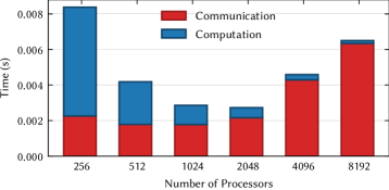
Figure 2.3. The time required for a single SpMV, split into communication and computation, for 2.1 run on Blue Waters with 16 processes per node.

Figure 2.4. Standard communication. On the left, Node 0 injects multiple messages into the network, all to P6 on Node 1. On the right, P1 sends multiple messages containing the same data to each process on Node 1, resulting in ”duplicate” data being sent across the network.

Node-aware communication techniques (Bienz et al., 2019, 2020) mitigate these issues by considering node topology to further break down the off-process block into vector values of $v$ that require on- or off-node communication; this decomposition is shown in Figure 2.2. As a result, costly redundant messages are traded for faster, on-node communication, resulting in 2 different multi-step schemes, namely 3-step and 2-step.

3-step Node-Aware Communication

3-step node-aware communication eliminates both redundancies in standard communication by gathering all necessary data to be sent off-node in a single buffer. Efficient implementation of this method relies on pairing all processes with a receiving process on distinct nodes – ensuring that every process remains active throughout the entire communication scheme.

First, all data to be sent to a separate node are gathered in a buffer by the single process paired with that node. Secondly, this process sends the data buffer to the paired process on the receiving node. Thirdly, the paired process on the receiving node redistributes the data locally to the correct destination processes on-node. An example of these steps is outlined in Figure 2.5.

Figure 2.5. 3-step node-aware. In Step 1, all the data on Node 0 that needs to be sent to Node 1 is collected in a buffer on P0, the process paired to send and receive from Node 1. In Step 2, P0 sends this buffer from Node 0 to P7, to the receiving process on Node 1. In Step 3, P7 redistributes the data to the correct receiving processes on Node 1.

2-Step Node-Aware Communication

2-step node-aware communication eliminates the redundancy of sending duplicate data from standard communication and decreases the number of inter-node messages, but not to the same degree as 3-step communication. In this case, each process exchanges the information needed by the receiving node with their paired process directly. Then the receiving node redistributes the messages on-node as shown in Figure 2.6. While multiple messages are sent to the same node, the duplicate data being sent through the network is eliminated. Hence, the number of bytes communicated with 3-step and 2-step node-aware schemes is the same, and often yields a significant reduction over the amount of data being sent through the network with standard communication.

Figure 2.6. 2-Step node-aware. Each process on Node 0 is paired with a receiving process on Node 1. In Step 1, each process on Node 0 sends the data needed by any process on Node 1 to its paired process on Node 1. Here, P0 is sending to P4, P1 to P5, P2 to P6, and P3 to P7. In Step 2, each process on Node 1 redistributes the data received from Node 0 to the destination on on Node 1.

2.2.1. Node-Aware Communication Models

parameter	description	first use
$p$	number of processes	§2.2
nnz	number of nonzeros in $A$	§3
$\alpha$	network latency	(2.5)
$s$	maximum number of bytes sent by a process	(2.5)
$m$	maximum number of messages sent by a process	(2.5)
ppn	processes per node	(2.5)
$R_{N}$	network injection rate (B/s)	(2.5)
$R_{b}$	network rate (B/s)	(2.5)
$s_{\text{proc}}$	maximum number of bytes sent by a process	(2.8)
$s_{\text{node}}$	maximum number of bytes injected by a node	(2.8)
$m_{\text{proc$\rightarrow$node}}$	maximum number of nodes to which a processor sends	(2.8)
$m_{\text{node$\rightarrow$node}}$	maximum number of messages between two nodes	(2.7)
$s_{\text{node$\rightarrow$node}}$	maximum size of a message between two nodes	(2.7)

Table 1. Modeling parameters.

The max-rate model (Gropp et al., 2016) is used to quantify the efficiency of node-aware communication throughout the remainder of Sections 2 and 3. For clarity, all modeling parameters referenced throughout the remainder of the paper are defined in Table 1. The max-rate model is an improvement to the standard postal model of communication, accounting for injection limits into the network. The cost of sending messages from a symmetric multiprocessing (SMP) node is modeled as

(2.5) $$T=\alpha\cdot m+\max\left(\frac{\texttt{ppn}\cdot s}{R_{N}},\frac{s}{R_{b}}\right)$$

where $\alpha$ is the latency, $m$ is the number of messages sent by a single process on a given node, $s$ is the number of bytes sent by a single process on a given SMP node, ppn is the number of processes per node, $R_{N}$ is the rate at which a network interface card (NIC) can inject data into the network, and $R_{b}$ is the rate at which a process can transport data.

In the case of on-node messages, the injection rate is not present and the max-rate model reduces to the standard postal model for communication

(2.6) $$T=\alpha_{\ell}\cdot m+\frac{s}{R_{b,\ell}},$$

where $\alpha_{\ell}$ is the local or on-node latency and $R_{b,\ell}$ is the rate of sending a message on-node.

In (Bienz et al., 2020), the max-rate model is extended to 2-step and 3-step communication by splitting the model into inter-node and intra-node components. For 3-step, the communication model becomes

(2.7) $$T_{\text{total}}=\underbrace{\alpha\cdot\frac{m_{\text{node$\rightarrow$node}}}{\texttt{ppn}}+\max\left(\frac{s_{\text{node}}}{R_{N}},\frac{s_{\text{proc}}}{R_{b}}\right)}_{\text{inter-node}}+\underbrace{2\cdot\left(\alpha_{\ell}\cdot(\texttt{ppn}-1)+\frac{s_{\text{node$\rightarrow$node}}}{R_{b,\ell}}\right)}_{\text{intra-node}}$$

where $m_{\text{node$\rightarrow$node}}$ is the maximum number of messages communicated between any two nodes and $s_{\text{node$\rightarrow$node}}$ is the size of messages communicated between any two nodes.

For 2-step, this results in

(2.8) $$T_{\text{total}}=\underbrace{\alpha\cdot m_{\text{proc$\rightarrow$node}}+\max\left(\frac{s_{\text{node}}}{R_{N}},\frac{s_{\text{proc}}}{R_{b}}\right)}_{\text{inter-node}}+\underbrace{\alpha_{\ell}\cdot(\texttt{ppn}-1)+\frac{s_{\text{proc}}}{R_{b,\ell}}}_{\text{intra-node}}$$

where $s_{\text{node}}$ and $s_{\text{proc}}$ represent the maximum number of bytes injected by a single NIC and communicated by a single process from an SMP node, respectively, and $m_{\text{proc$\rightarrow$node}}$ is the maximum number of nodes with which any process communicates.

The latency to communicate between nodes, $\alpha$, is often much higher than the intra-node latency, $\alpha_{\ell}$, thus motivating a multi-step communication approach. In a 2-step method, having every process on-node communicate data minimizes the constant factor $\max\left(\frac{s_{\text{node}}}{R_{N}},\frac{s_{\text{proc}}}{R_{b}}\right)$, which depends on the maximum amount of data being communicated to a separate node by a single process. In practice, a 3-step method often yields the best performance for a parallel SpMV since the amount of data being communicated by a single process is often small. As a result moving the data to be communicated off-node into a single buffer minimizes the first term in Equation 2.7. These multi-step communication techniques minimize the amount of time spent in inter-node communication. We extend this idea to the block vector operation in Section 4.1.

3. Performance Study of Enlarged Conjugate Gradient

In this section we detail the per-iteration performance and performance modeling of ECG. A communication efficient version of Algorithm 2.1 is implemented in Raptor (Bienz and Olson, 2017) and is based on the work in (Grigori and Tissot, 2019). Throughout this section and the remainder of the paper, we assume an $n\times n$ matrix $A$ with nnz nonzeros is partitioned row-wise across a set of $p$ processes. Each process contains at most $\frac{n}{p}$ contiguous rows of the matrix $A$. In the modeling that follows, we assume a equal number of nonzeros per partition. In addition, each block vector in Algorithm 2.1 — $R$, $X$, $Z$, $AZ$, $P$, and $AP$ — is partitioned row-wise, and with the same row distribution as $A$. The variables $c$, $d$, and $d_{\text{\tiny old}}$ are size $t\times t$ and a copy of each is stored locally on each process. Tests were performed on the Blue Waters Cray XE/XK machine at the National Center for Supercomputing Applications (NCSA) at University of Illinois. Blue Waters (Bode et al., 2013; Kramer et al., 2015) contains a 3D torus Gemini interconnect; each Gemini consists of two nodes. The complete system contains 22 636 XE compute nodes; each with two AMD 6276 Interlagos processors, and additional XK compute nodes unused in these tests.

3.1. Implementation

The scalability of a direct implementation of Algorithm 2.1 is limited (Grigori and Tissot, 2019), however, this is improved by fusing communication and by executing the system solve in Algorithm 2.1 in Algorithm 2.1 on each process. This is accomplished in (Grigori and Tissot, 2019) by decomposing the computation of $P$ into several steps as described in Algorithm 3.1.

$AZ\leftarrow A*Z$

  [sparse matrix-block vector multiplication]

$Z^{T}AZ\leftarrow Z^{T}*AZ$

  [$t$ inner products]

$C^{T}C\leftarrow Z^{T}AZ$

  [Cholesky factorization]

$P\leftarrow\text{solve}\,P*C=Z$

  [Triangular solve with multiple right sides]

Algorithm 3.1 Calculating $P:=Z(Z^{T}AZ)^{-1/2}$

The $t\times t$ product $Z^{T}(AZ)$ is stored locally on every process in the storage space of $c$, as shown in Figure 3.1. The Cholesky factorization on Algorithm 3.1 of Algorithm 3.1 is performed simultaneously on every process, yielding a (local) copy of $C$. Then each process performs a local triangular system solve using the local vector values of $Z$ to construct the portion of $P$ (see Algorithm 3.1). Similarly, an additional sparse matrix block vector product $AP=A*P$ is avoided by noting that $AP$ is constructed using

$$AP\leftarrow\texttt{Triangular Solve with Multiple Right Sides of }AP*C=AZ$$

since the product $AZ$ and the previous iteration’s $AP=A*P$ are already stored.

Figure 3.1. The above figure displays the partitioning of all the vectors and intermediary Partition of vectors $R$, $X$, $Z$, $AZ$, $P$, and $AP$ along with $t\times t$ working arrays $c$, $d$, and $d_{\text{\tiny old}}$, as in Algorithm 2.1, for $t=2$.

Algorithm 3.2 summarizes our implementation in terms of computational kernels, with the on process computation in terms of floating point operations along with the associated type of communication. The remainder of the calculations within ECG consist of local block vector updates, as well as block vector inner products for the values $c$, $d$, and $d_{\text{\tiny old}}$. A straightforward approach is to compute these independently within the algorithm, resulting in four MPI_Allreduce global communications per iteration. However, since the input data required to calculate $c$, $d$, and $d_{\text{\tiny old}}$ are available on Algorithm 2.1 in Algorithm 2.1 when $c$ is computed, a single global reduction is possible. The implementation described in Algorithm 3.2 highlights a single call to MPI_Allreduce for all of these values and reducing them in the same buffer. This reduces the number of MPI_Allreduce calls to two per iteration.

1 SpMV

2 Vector Initialization

3 for $k=1,\dots$ 

      SpMBV

        $\rightarrow$ $2\cdot\frac{\texttt{nnz}}{p}\cdot t$     Comm: point-to-point

       Block inner product

        $\rightarrow$ $2\cdot\frac{n}{p}\cdot t^{2}$       Comm: global all reduce

       Cholesky decomposition

        $\rightarrow$ $\frac{1}{6}\cdot t^{3}$

       Triangular solves

        $\rightarrow$ $2\cdot\frac{1}{2}\cdot t^{2}$

       Block inner product

        $\rightarrow$ $2\cdot\frac{n}{p}\cdot t^{2}$       Comm: global all reduce

       Block vector addition

        $\rightarrow$ $2\cdot\frac{n}{p}\cdot t$

       Block vector axpy

        $\rightarrow$ $2\cdot\frac{n}{p}\cdot t$

4      

Algorithm 3.2 Enlarged Conjugate Gradient by Kernel

From Algorithm 3.2, we note that computation and communication per iteration costs of ECG have increased over that of parallel CG. For our implementation, the number of collective communication calls to MPI_Allreduce has remained the same as CG (at two), but the number of values in the global reductions has increased from a single float in each of CG’s global reductions to $t^{2}$ and $3t^{2}$. The singular SpMV from CG has increased to a sparse matrix block vector product (SpMBV), which does not increase the number of point-to-point messages, but does increase the size of the messages being communicated by the enlarging factor $t$. Additionally, the local computation for each kernel has increased by a factor of $t$. ECG uses these extra per iteration requirements to reduce the total number of iterations to convergence, resulting in fewer iterations than CG as seen in Figure 3.2.

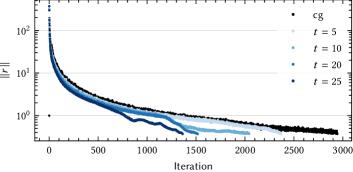
Figure 3.2. Residual history for CG and ECG with various enlarging factors $t$ for 2.1.

3.2. Per Iteration Performance

In Figure 3.3 we decompose the performance of a single iteration of ECG for 2.1 into (local) computation, point-to-point communication, and collective communication. Performance tests were executed on Blue Waters (Bode et al., 2013; Kramer et al., 2015). Each test is the average of 20 iterations of ECG; reported times are the maximum average time recorded for any single process. At small scales, local computation dominates performance, while at larger scales, the point-to-point communication in the single SpMBV kernel and the collective communication in the block vector inner products become the bottleneck in ECG. Figure 3.3 also shows the time spent in a single inner product. While we observe growth with the number of processes, as expected, the relative cost (and growth) within ECG remains low. Importantly, increasing $t$ at high processor counts does not significantly contribute to cost. This is shown in Figure 3.4, where the mean runtime for various block vector inner products all fall within each other’s confidence intervals. This suggests that increasing $t$ to drive down the iteration count will have little affect on the per iteration cost of the two calls to MPI_Allreduce, and in fact, will result in fewer total calls to it due to the reduction in iterations.

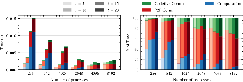
Figure 3.3. Time (left) and percentage of time (right) for a single iteration of ECG for various block vector sizes, $t$, and processor counts for 2.1. The three varying shades for each $t$ value represent the amount of overall time spent in on-process computation point-to-point communication, and collective communication.

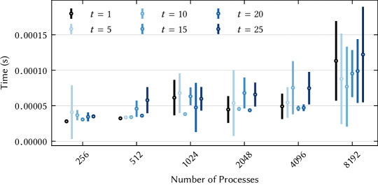
Figure 3.4. Time for a single inner product (right) for various block vector sizes, $t$, and processor counts for 2.1. Vertical lines denote the confidence intervals.

The remainder of this section focuses on accurately predicting the performance of a single iteration of ECG through robust performance models. In particularly, SpMBV communication is addressed in detail in Section 4 where we discuss new node-aware communication techniques for blocked data.

3.3. Performance Modeling

To better understand the timing profiles in Figure 3.3, we develop performance models. Below, we present two different models for the performance of communication within a single iteration of ECG. First, consider the standard postal model for communication, which represents the maximum amount of time required for communication by an individual process in a single iteration of ECG as

(3.1) $$T_{\text{postal}}=\underbrace{\alpha\cdot m+\frac{s\cdot t}{R_{b}}}_{\text{point to point}}+\underbrace{2\cdot\alpha\cdot\log(p)+\frac{f\cdot 4\cdot t^{2}}{R_{b}}}_{\text{collective}}$$

where $f$ is the number of bytes for a floating point number — e.g. $f=8$. See Table 1 for a complete description of model parameters. As discussed in Section 2.2.1, this model presents a misleading picture on the performance of ECG at scale, particularly on current supercomputer architectures where SMP nodes encounter injection bandwidth limits when sending inter-node messages.

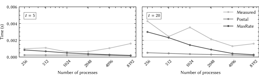
Figure 3.5. Max-rate model versus the postal model for the point to point communication in one iteration of ECG for 2.1 using various $t$. Measured runtimes are also included. (note: $t=5$ and $t=20$ shown for brevity).

To improve the model we drop in the max-rate model for the point-to-point communication, resulting in

(3.2) $$T_{MR}=\underbrace{\alpha\cdot m+\max\left(\frac{\texttt{ppn}\cdot s\cdot t}{R_{N}},\frac{s\cdot t}{R_{b}}\right)}_{\text{point to point}}+\underbrace{2\cdot\alpha\cdot\log(p)+\frac{f\cdot 4\cdot t^{2}}{R_{b}}}_{\text{collective}}.$$

Figure 3.5 shows that the max-rate model provides a more accurate upper bound on the time spent in point to point communication within ECG. The term $2\cdot\alpha\cdot\log(p)+\frac{f\cdot 4\cdot t^{2}}{R_{b}}$ remains unchanged in Equations 3.1 and 3.2 to represent the collective communication required for the two block vector inner products. Each block vector inner product incurs latency from requiring $\log(p)$ messages in an optimal implementation of the MPI_Allreduce. More accurate models for modeling the communication of the MPI_Allreduce in the inner product exist, such as the logP model (Culler et al., 1993) and logGP model (Alexandrov et al., 1997), but optimization of the reduction is outside the scope of this paper, so we leave the postal model for representing the performance of the inner products.

Modeling the computation within an iteration of ECG is straightforward. The computation for a single iteration of ECG is written as the sum of the kernel floating point operations in Algorithm 3.2, which results in the following

(3.3) $$T_{comp}=\gamma\cdot\left((2+2t)\frac{\texttt{nnz}}{p}+(4t+4t^{2})\frac{n}{p}+\frac{1}{2}t^{2}+\frac{1}{6}t^{3}\right)$$

where $\gamma$ is the time required to compute a single floating point operation. In total, we arrive at the following model for a single iteration of ECG

(3.4) $$T_{ECG}=\alpha\cdot m+\max\left(\frac{\texttt{ppn}\cdot s\cdot t}{R_{N}},\frac{s\cdot t}{R_{b}}\right)+2\cdot\alpha\cdot\log(p)+\frac{f\cdot 4\cdot t^{2}}{R_{b}}+\gamma\cdot\left((2+2t)\frac{\texttt{nnz}}{p}+(4t+4t^{2})\frac{n}{p}+\frac{1}{2}t^{2}+\frac{1}{6}t^{3}\right).$$

Using this model, we can predict the reduction in the amount of time spent in point-to-point communication using the multi-step communication techniques presented in Section 2.2.1 for a single iteration of ECG for 2.1 — see Table 2.

procs $\rightarrow$	256		512		1024		2048		4096		8192
$t$	m-s	std	m-s	std	m-s	std	m-s	std	m-s	std	m-s	std
5	42.2	55.6	57.9	70.0	71.7	70.2	80.1	75.5	83.5	78.9	81.9	76.6
10	21.2	40.0	34.5	56.2	51.2	65.2	65.9	67.5	75.9	69.1	77.7	68.7
15	13.0	37.6	22.2	40.4	35.2	66.7	48.6	67.0	60.0	58.5	60.5	63.8
20	9.3	24.5	16.5	38.3	27.4	62.3	40.6	47.6	54.4	45.5	57.2	53.6

(a) 2-Step Communication

procs $\rightarrow$	256		512		1024		2048		4096		8192
$t$	m-s	std	m-s	std	m-s	std	m-s	std	m-s	std	m-s	std
5	29.6	55.6	43.0	70.0	54.8	70.2	64.2	75.5	72.3	78.9	71.4	76.6
10	14.6	40.0	24.4	56.2	35.9	65.2	49.5	67.5	65.6	69.1	68.5	68.7
15	9.2	37.6	15.8	40.4	23.9	66.7	34.4	67.0	49.9	58.5	50.8	63.8
20	6.7	24.5	11.9	38.3	18.6	62.3	28.7	47.6	45.9	45.5	48.8	53.6

(b) 3-Step Communication

Table 2. Modeled percentage of time to be spent in point-to-point communication for multistep (“m-s”) compared against the measured percentage of time spent in point-to-point communication for standard (“std”) in a single iteration of ECG for 2.1 with varying $t$ and processor counts on Blue Waters. Blue values correspond to values for which the percentage of time decreased by $5\%-20\%$, green values are a decrease of over $20\%$, and red values predict an increase over the original percentage.

We see that ECG is still limited at large processor counts even when substituting the node-aware communication techniques to replace the costly point-to-point communication observed in Figure 3.3. The models do predict a large amount of speedup for most cases, however, when using 3-step communication, suggesting that node-aware communication techniques can reduce the large point-to-point bottleneck observed in the performance study. While a large communication cost stems equally from the collective communication the MPI_Allreduce operations, their performance is dependent upon underlying MPI implementation and outside the scope of this paper. We address the point-to-point communication performance further in Section 4 by analyzing it through the lens of node-aware communication techniques, optimizing them to achieve the best possible performance at scale.

4. Optimized Communication for Blocked Data

As discussed in Section 3, scalability for ECG is limited by the sparse matrix-block vector multiplication (SpMBV) kernel defined as

(4.1) $$A\cdot V\rightarrow W,$$

with $A\in\mathbb{R}^{n\times n}$ and $V$, $V\in\mathbb{R}^{n\times t}$, where $1<t\ll n$. Due to the block vector structure of $X$, each message in a SpMV is increased by a factor of $t$ (see Figure 4.1). The larger messages associated with $t>1$ increase the amount of time spent in the point-to-point communication at larger scales, making the SpMBV operation an ideal candidate for node-aware messaging approaches.

Figure 4.1. Sparse matrix-block vector multiplication (cf. Figure 2.2).

4.1. Performance Modeling

Recalling the node-aware communication models from Section 2.2.1, we augment the 2-step and 3-step models with block vector size, $t$. As a result, the 2-step model in Equation 2.8 becomes

(4.2) $$T_{total}=\underbrace{\alpha\cdot m_{\text{proc$\rightarrow$node}}+\max\left(\frac{t\cdot s_{\text{node}}}{R_{N}},\frac{t\cdot s_{\text{proc}}}{R_{b}}\right)}_{\text{inter-node}}+\underbrace{\alpha_{\ell}\cdot(\texttt{ppn}-1)+t\cdot\frac{s_{\text{proc}}}{R_{b,\ell}}}_{\text{intra-node}}$$

while the 3-step model in Equation 2.7 becomes

(4.3) $$T_{total}=\underbrace{\alpha\cdot\frac{m_{\text{node$\rightarrow$node}}}{\texttt{ppn}}+\max\left(\frac{t\cdot s_{\text{node}}}{R_{N}},\frac{t\cdot s_{\text{proc}}}{R_{b}}\right)}_{\text{inter-node}}+\underbrace{2\cdot\left(\alpha_{\ell}\cdot(\texttt{ppn}-1)+t\cdot\frac{s_{\text{node$\rightarrow$node}}}{R_{b,\ell}}\right)}_{\text{intra-node}}.$$

In both models, $t$ impacts maximum rate, a term that is relatively small for $t=1$ and dominates the inter-node portion of the communication as $t$ grows. Since messages are increased by a factor of $t$, the single buffer used in 3-step communication quickly reaches the network injection bandwidth limits. Using multiple buffers, as in 2-step communication, helps mitigate the issue, however more severe imbalance persists since the amount of data sent to different nodes is often widely varying.

Figure 4.2 shows every inter-node message sent by a single process alongside the message size for 2.1 when performing the SpMBV kernel with 4096 processes and 16 processes per node. We present the message sizes for 3-step and 2-step communication, noting that the overall number of inter-node messages decreases when using 3-step communication, but the average message size sent by a single process increases.

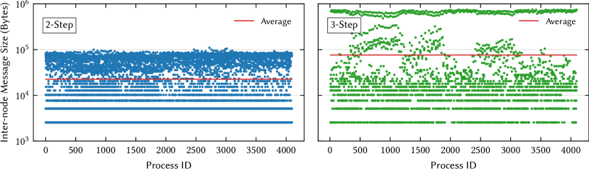
Figure 4.2. The inter-node message sizes across all processes for 2-Step and 3-step communication when performing the SpMBV for 2.1 when $t=20$ across 4096 processes on Blue Waters. The average message size across all processes is marked by a red line.

For $t=20$, the maximum message size nears $10^{6}$ for 3-step communication, while the maximum message size barely reaches $10^{5}$ for 2-step communication. Additionally, there is clear imbalance in the inter-node message sizes for 2-step communication with messages ranging in size from $10^{3}$–$10^{5}$ Bytes.

4.2. Profiling

We next apply the node-aware communication strategies presented for SpMVs and SpGEMMs in Section 2.2 to the SpMBV kernel within ECG.

Figure 4.3 displays the performance of standard, 2-step, and 3-step communication when applied to the SpMBV kernel for 2.1 with $t=5$ and $t=20$. The 2-step communication appears outperform in most cases. This is due to the large amount of data to be sent off-node that is split across many processes. We see 2-step communication performing better due to the term $\alpha\cdot m_{\text{proc$\rightarrow$node}}$ in Equation 4.2 being smaller than the $\alpha\cdot m_{\text{node$\rightarrow$node}}$ term in the 3-step communication model Equation 4.3 due to multiplication by the factor $t$. In fact, all counts measured in the ECG profiling section are now multiplied by the enlarging factor $t$. While the traditional SpMV shows speedup with 3-step communication, we now see that 2-step is generally the best fit for our methods as message size, and thus $t$, increases.

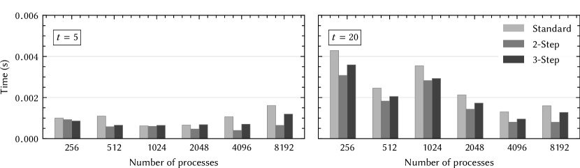
Figure 4.3. Strong scaling results for 2.1 using standard, 2-step, and 3-step communication in the SpMBV (note: $t=5$ and $t=20$ shown for brevity).

Next we consider node-aware communication performance results for a subset of the largest matrices in the SuiteSparse matrix collection (Davis and Hu, 2011) (matrix details can be found in Table 3). These were selected based on size and density to provide a variety of scenarios.

matrix	rows/ cols	nnz	nnz/row	density
audikw_1	$943\,695$	$77\,651\,847$	82.3	8.72e-5
Geo_1438	$1\,437\,960$	$60\,236\,322$	41.9	2.91e-05
bone010	$986\,703$	$47\,851\,783$	48.5	4.92e-05
Emilia_923	$923\,136$	$40\,373\,538$	43.7	4.74e-05
Flan_1565	$1\,565\,794$	$114\,165\,372$	72.9	4.66e-05
Hook_1498	$1\,498\,023$	$59\,374\,451$	39.6	2.65e-05
ldoor	$952\,203$	$42\,493\,817$	44.6	4.69e-05
Serena	$1\,391\,349$	$64\,131\,971$	46.1	3.31e-05
thermal2	$1\,228\,045$	$8\,580\,313$	7.0	5.69e-06

Table 3. Test Matrices.

While 2-step communication is effective in many instances, it is not always the most optimal communication strategy, as depicted in Figure 4.4. Unlike the results for 2.1, 3-step and 2-step communication do not always outperform standard communication, and in some instances (4096 processes), for most values of $t$ there is performance degradation. This is seen more clearly in Figure 4.5.

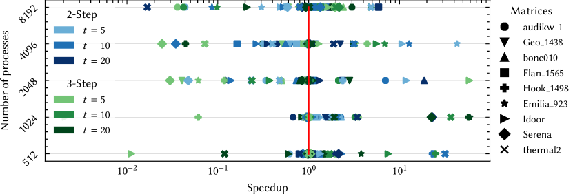
Figure 4.4. Speedup of 2-step and 3-step communication over standard communication in the SpMBV for various matrices from the SuiteSparse matrix collection on Blue Waters. The red line marks 1.0, or no speedup.

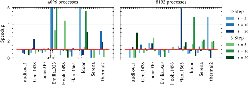
Figure 4.5. Speedup of 2-step and 3-step communication over standard communication in the SpMBV for various matrices on Blue Waters for 4096 and 8192 processes. The red line marks 1.0, or no speedup. Speedups greater than 6.0 are given via annotations on the plot.

It is important to highlight cases where only a single node-aware communication technique results in performance deterioration over standard communication. Distinct examples include Geo_1438 and thermal2 on 4096 processes. Both of these matrices benefit from 2-step communication for $t=10$ and $20$, but performance degrades when using 3-step communication. Another example is the performance of ldoor on 8192 processes (seen in Figure 4.5). For $t=5$ and $10$, ldoor results in performance degradation using 2-step communication, but up to $5\times$ speedup over standard communication when using 3-step communication. These cases highlight that while one node-aware communication technique underperforms in comparison to standard communication, the other node aware technique is still much faster. Using this as the key motivating factor, we discuss an optimal node-aware communication technique for blocked data in Section 4.3.

4.3. Optimal Communication for Blocked Data

When designing an optimal communication scheme for the blocked data format, the main consideration is the impact the number of vectors within the block have on the size of messages communicated. The effects message size and message number have on performance can vary based on machine, hence we present results for Blue Waters alongside Lassen (Hanson, 2020). Lassen, a 23-petaflop IBM system at Lawrence Livermore National Laboratory, consists of 792 nodes connected via a Mellanox 100 Gb/s Enhanced Data Rate (EDR) InfiniBand network. Each node on Lassen is dual-socket with 44 IBM Power9 cores and 4 NVIDIA Volta GPUs (which are unused in our tests.)

In Figure 4.6, we view the effects placement of data and amount of data being communicated has on performance times for two different machines. This figure shows the amount of time required to send various numbers of bytes between two processes when they are located on the same node but different sockets (blue) and on the same node and same socket (red) for the machines Blue Waters (left) and Lassen (right). It also shows the amount of time required to communicate between two processes on separate nodes when there are less than 4 (Blue Waters) or 5 (Lassen) active processes communicating through the network at the same time or greater than 4 or 5 processes communicating through the network at the same time. We see that as the number of bytes communicated between two processes increases, it becomes increasingly important whether those two processes are located on the same socket, node, or require communication through the network.

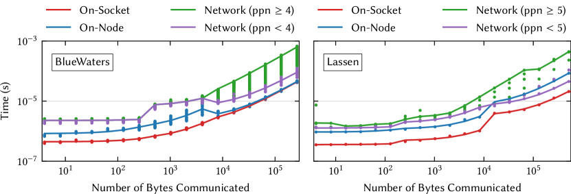
Figure 4.6. Communication time on-socket, on-node, or across the network on Blue Waters (left) and Lassen (right). Measured times are displayed as dots; solid lines represent max-rate model (Gropp et al., 2016). ppn represents the number of processors participating in communication. (The Blue Waters data was initially presented in (Bienz et al., 2018) and is replotted here.)

For both machines, inter-node communication is fastest when message sizes are small, and there are few messages being injected into the network. On Blue Waters, intra-node communication is the fastest, with the time being dependent on how physically close the processes are located. For instance, when two processes are on the same socket, communication is faster than when they are on the same node, but different sockets. This is true for Lassen, as well, but cross-socket intra-node communication is not always faster than communicating through the network. Once message sizes exceed $10^{4}$ bytes, and there are fewer than five processes actively communicating, inter-node communication is faster than two cross-socket intra-node processes communicating. For both machines, however, we see that once a large enough communication volume is reached, it becomes faster to split the inter-node data being sent across a subset of the processes on a single node due to network contention as observed in (Bienz et al., 2018).

In addition to the importance of the placement of two communicating processes, the total message volume and number of actively communicating processes plays a key role in communication performance. While it is extremely costly for every process on a node to send $10^{5}$ bytes as seen in Figure 4.6, there are performance benefits when splitting a large communication volume across all processes on a node, depicted in Figure 4.7. Blue Waters sees modest performance benefits when splitting large messages across multiple processes, whereas Lassen sees much greater performance benefits.

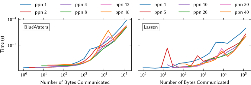
Figure 4.7. Time required to send data between two processes on separate nodes with the data communication split across ppn processes. Timings for Blue Waters and Lassen are presented in the left and right plots, respectively.

These observations help justify why 3-step communication would outperform 2-step communication, and vice versa in certain cases of the SpMBV profiling presented in Figure 3.5. Sending all messages in a single buffer becomes impractical when the block size, $t$, is very large, but having each process communicate with a paired process also poses problems when some of the inter-node messages being sent are still very large, as seen in Figure 4.2.

Motivated by the results above, we introduce an optimized multi-step communication process that combines the aspects of both the 3-step and 2-step communication techniques, and using 3-step or 2-step communication when necessary. We reduce the number of inter-node messages and conglomerate messages to be sent off node for certain cases when the message sizes to be sent off-node are below a given threshold, and we split the messages to be sent off-node across multiple processes when the message size is larger than a given threshold. Hence, each node is determining the most optimal way to perform its inter-node communication. As a result, this nodal optimal communication eliminates the redundancies of data being injected into the network, just as 3-step and 2-step do, but in some cases, it does not reduce the number of inter-node messages as much as 3-step, and in fact can increase the number of inter-node messages injected by a single node to be larger than those injected by 2-step, but never exceeding the total number of active processes per node.

The number of inter-node messages sent can be represented by the following inequality,

(4.4) $$m_{\text{node$\rightarrow$node}}\leq n_{opt}\leq\max(m_{\text{proc$\rightarrow$node}},\texttt{ppn})$$

where $n_{opt}$ is the number of inter-node messages injected by a single process for the optimal node-aware communication, and it is bounded below by the worst-case number of messages communicated in 3-step communication Equation 4.3 and above by the worst-case number of messages communicated in 2-step communication Equation 4.2 or ppn, whichever is greater.

The proposed process, excluding reducing the global communication strategy to 3-step or 2-step communication, is summarized in Figure 4.8. This figure outlines the nodal optimal process of communicating data between two nodes, each with four local processes.

Step 1::

Each node conglomerates small messages to be sent off-node while retaining larger messages. Messages are assigned to processes in descending order of size to the first available process on node. This is done for every node simultaneously.

Step 2::

Buffers prepared in step 1 are sent to their destination node, specifically to the paired process on that node with the same local rank. P0 exchanges data with P4, while P1 sends data to P5, and P2 sends data to P6.

Step 3::

All processes on each individual node redistribute their received data to the correct destination processes on-node. In this step, all communication is local.

Figure 4.8. Node-aware communication on two nodes with four processes each.

The resulting speedups for the two systems Blue Waters and Lassen are presented in Figure 4.9. Here, the message size cutoff being used is the message size cutoff before the MPI implementation switches to the rendezvous protocol. For sending large messages between processes, the rendezvous protocol communicates an envelope first, then the remaining data is communicated after the receiving process allocates buffer space. It is necessary to use this protocol for large messages, but there is a slight slowdown over sending messages via the short and eager protocols which either include the data being sent as part of the envelope (short) or eagerly send the data if it does not fit into the envelope (eager). This cutoff is chosen because rendezvous is the slowest protocol and because the switch to the rendezvous protocol is approximately the crossover point when on-node messages become slower than network messages on Lassen (around $10^{4}$ Bytes in Figure 4.6.)

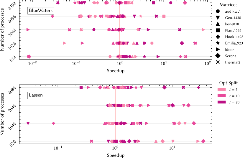
Figure 4.9. Speedup of optimal communication over standard communication (without reducing to a global communication strategy) in the SpMBV for various matrices from the SuiteSparse matrix collection on Blue Waters and Lassen. The red line marks 1, or no speedup.

Using this cutoff point, the method sees speedup for some test matrices and performance degradation for most on Blue Waters, which is consistent with the minimal speedup seen by splitting large messages across multiple processes in Figure 4.7. Additionally, it is likely that network contention is playing a large role in the Blue Waters results as the messages sizes become large based on the findings in (Bienz et al., 2018), and due to each node determining independently how to send its own data without consideration of the size or number of messages injected by other nodes.

The nodal optimal communication performs better on Lassen than Blue Waters and aligns with expectations based on the combination of using 3-step for nodes with small inter-node messages to inject into the network where on-node communication is faster than network communication (Figure 4.6) and splitting large messages where the benefits are much greater (Figure 4.7). While Blue Waters achieves higher speedups in some cases than Lassen, both systems see speedups as large as 60x. These results only present part of the overall communication picture, however. There are still cases where the global communication strategy should be reduced to 3-step communication, 2-step communication, or standard communication. This differs based on the two machines and the specific test matrix, but tuning between the techniques results in the most optimal communication strategy. Tuning comes at the minimal cost of performing four different SpMBVs during setup of the SpMBV communicator. Speedups over standard communication when using tuning to use the fastest communication technique are presented in Figure 4.10.

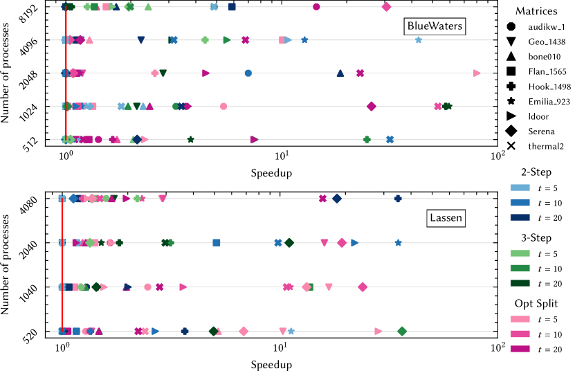
Figure 4.10. Speedup of tuned communication over standard communication in the SpMBV for various matrices from the SuiteSparse matrix collection on Blue Waters and Lassen. The red line marks 1.0, or no speedup.

In the top plot of Figure 4.10, Blue Waters benefits in 33% of the cases from including the nodal optimal multi-step communication strategy. These results are expected based on Figure 4.9 where the benefits of nodal optimal multi-step communication were less than ideal. In fact, for 20% of the cases on Blue Waters, standard communication is the most performant, consistent with matrices of low density. The matrices Geo_1438 and ldoor, which have the smallest density of the test matrices (Table 3), see minimal benefits from the multi-step communication techniques as the number of processes is scaled up due to the minimal amount of data being communicated.

We expected to see 2-step and nodal optimal communication perform the best on Lassen due to the faster inter-node communication for smaller sized messages (Figure 4.6) and the benefits of splitting messages across many processes on node (Figure 4.7). These expectations are consistent with the results presented in the bottom plot of Figure 4.10; most test matrices saw the best SpMBV performance with nodal optimal communication (44% of the cases). The remainder of the test cases were divided almost equally between 2-step, 3-step, and standard communication for which technique was the most performant (approximately 18% of the cases, each).

Table 4 shows the benefits of using the tuned point-to-point communication over the standard communication in a single iteration of ECG for 2.1. Tuned communication reduces the percentage of time spent in point-to-point communication independent of system, though the performance benefits are typically best when more data is being communicated ($t=20$ in Table 4(a) and Table 4(b).) For Blue Waters, the new communication technique results in point-to-point communication taking $20\%-40\%$ less of the total time compared to the percentage of time when using standard communication (corresponding to the blue highlighted values in Table 4(a)). Performance benefits are much greater on Lassen where the tuned communication results in a decrease of more than $40\%$ of the total iteration time compared to an iteration time with standard communication in most cases.

procs $\rightarrow$	256		512		1024		2048		4096		8192
$t$	m-s	std	m-s	std	m-s	std	m-s	std	m-s	std	m-s	std
5	54.7	55.6	34.1	70.0	66.2	70.2	70.6	75.5	70.2	78.9	41.7	76.6
10	31.8	40.0	39.3	56.2	34.6	65.2	48.4	67.5	59.7	69.1	32.2	68.7
15	9.3	37.6	18.2	40.4	30.4	66.7	31.9	67.0	38.4	58.5	26.0	63.8
20	7.5	24.5	15.0	38.3	26.3	62.3	46.0	47.6	30.8	45.5	29.7	53.6

(a) Blue Waters

procs $\rightarrow$	240		520		1040		2040		4080
$t$	m-s	std	m-s	std	m-s	std	m-s	std	m-s	std
5	49.4	84.3	43.6	88.0	66.6	88.4	82.2	87.2	82.7	93.1
10	26.8	87.2	33.7	84.9	52.1	84.7	58.4	89.3	78.3	91.3
15	9.9	81.2	26.4	85.7	33.6	86.1	55.3	90.0	61.2	89.2
20	12.7	74.2	17.8	79.9	29.6	81.7	39.0	80.7	57.2	79.5

(b) Lassen

Table 4. Measured percentage of time spent in point-to-point communication for the tuned multistep (“m-s”) compared against the measured percentage of time spent in point-to-point communication for standard (“std”) in a single iteration of ECG for 2.1 with varying $t$ and processor counts on Blue Waters and Lassen. Blue values correspond to values for which the percentage of time decreased by $5\%-20\%$, green values are a decrease of $20\%-40\%$, and yellow values decreased by more than 40% from the original percentage.

5. Conclusions

The enlarged conjugate gradient method (ECG) is an efficient method for solving large systems of equations designed to reduce the collective communication bottlenecks of the classical conjugate gradient method (CG.) Within ECG, block vector updates replace the single vector updates of CG, thereby reducing the overall number of iterations required for convergence and hence the overall amount of collective communication.

In this paper, we performed a performance study and analysis of the effects of block vectors on the balance of collective communication, point-to-point communication, and computation within the iterations of ECG. We noted the increased volume of data communicated and its disproportionate affects on the performance of the point-to-point communication; the communication bottleneck of ECG shifted to be the point-to-point communication within the sparse matrix-block vector kernel (SpMBV). To address the new SpMBV bottleneck, we designed an optimal multi-step communication technique that builds on existing node-aware communication techniques and improves them for the emerging supercomputer architectures with greater numbers of processes per node and faster inter-node networks.

Overall, this paper provides a comprehensive study of the performance of ECG in a distributed parallel environment, and introduces a novel point-to-point multi-step communication technique that provides consistent speedup over standard communication techniques independent of machine. Future work includes profiling and improving the performance of ECG on hybrid supercomputer architectures with computation offloaded to graphics processing units.

The software used to generate the results in this paper is freely available in RAPtor (Bienz and Olson, 2017).

References

- (1)
- Alexandrov et al. (1997) Albert Alexandrov, Mihai F. Ionescu, Klaus E. Schauser, and Chris Scheiman. 1997. LogGP: Incorporating Long Messages into the LogP Model for Parallel Computation. J. Parallel and Distrib. Comput. 44, 1 (1997), 71 – 79. https://doi.org/10.1006/jpdc.1997.1346
- Anderson et al. (2020) Robert Anderson, Julian Andrej, Andrew Barker, Jamie Bramwell, Jean-Sylvain Camier, Jakub Cerveny, Veselin Dobrev, Yohann Dudouit, Aaron Fisher, Tzanio Kolev, Will Pazner, Mark Stowell, Vladimir Tomov, Ido Akkerman, Johann Dahm, David Medina, and Stefano Zampini. 2020. MFEM: A modular finite element methods library. Computers & Mathematics with Applications (2020). https://doi.org/10.1016/j.camwa.2020.06.009
- Bienz et al. (2019) Amanda Bienz, William Gropp, and Luke Olson. 2019. Node aware sparse matrix–vector multiplication. J. Parallel and Distrib. Comput. 130 (08 2019), 166–178. https://doi.org/10.1016/j.jpdc.2019.03.016
- Bienz et al. (2018) Amanda Bienz, William D. Gropp, and Luke N. Olson. 2018. Improving Performance Models for Irregular Point-to-Point Communication. CoRR abs/1806.02030 (2018). http://arxiv.org/abs/1806.02030
- Bienz et al. (2020) Amanda Bienz, William D Gropp, and Luke N Olson. 2020. Reducing communication in algebraic multigrid with multi-step node aware communication. The International Journal of High Performance Computing Applications 34, 5 (June 2020), 547–561. https://doi.org/10.1177/1094342020925535
- Bienz and Olson (2017) Amanda Bienz and Luke N. Olson. 2017. RAPtor: parallel algebraic multigrid v0.1. https://github.com/raptor-library/raptor. Release 0.1.
- Bode et al. (2013) Brett Bode, Michelle Butler, Thom Dunning, Torsten Hoefler, William Kramer, William Gropp, and Wen-mei Hwu. 2013. The Blue Waters Super-System for Super-Science. In Contemporary High Performance Computing. Chapman and Hall/CRC, 339–366. https://www.taylorfrancis.com/books/e/9781466568358
- Carson et al. (2013) Erin Carson, Nicholas Knight, and James Demmel. 2013. Avoiding Communication in Nonsymmetric Lanczos-Based Krylov Subspace Methods. SIAM J. Sci. Comput. 35, 5 (Jan. 2013), S42–S61. https://doi.org/10.1137/120881191 arXiv:https://doi.org/10.1137/120881191
- Chronopoulos and Gear (1989) A.T. Chronopoulos and C.W. Gear. 1989. s-step iterative methods for symmetric linear systems. J. Comput. Appl. Math. 25, 2 (Feb. 1989), 153–168. https://doi.org/10.1016/0377-0427(89)90045-9
- Cools and Vanroose (2017) S. Cools and W. Vanroose. 2017. The communication-hiding pipelined BiCGstab method for the parallel solution of large unsymmetric linear systems. Parallel Comput. 65 (July 2017), 1–20. https://doi.org/10.1016/j.parco.2017.04.005
- Culler et al. (1993) David Culler, Richard Karp, David Patterson, Abhijit Sahay, Klaus Erik Schauser, Eunice Santos, Ramesh Subramonian, and Thorsten von Eicken. 1993. LogP: Towards a Realistic Model of Parallel Computation. SIGPLAN Not. 28, 7 (July 1993), 1–12. https://doi.org/10.1145/173284.155333
- Davis and Hu (2011) Timothy A. Davis and Yifan Hu. 2011. The University of Florida Sparse Matrix Collection. ACM Trans. Math. Softw. 38, 1, Article 1 (Dec. 2011), 25 pages. https://doi.org/10.1145/2049662.2049663
- Ghysels and Vanroose (2014) P. Ghysels and W. Vanroose. 2014. Hiding global synchronization latency in the preconditioned Conjugate Gradient algorithm. Parallel Comput. 40, 7 (July 2014), 224–238. https://doi.org/10.1016/j.parco.2013.06.001
- Grigori et al. (2016) Laura Grigori, Sophie Moufawad, and Frederic Nataf. 2016. Enlarged Krylov Subspace Conjugate Gradient Methods for Reducing Communication. SIAM J. Matrix Anal. & Appl. 37, 2 (Jan. 2016), 744–773. https://doi.org/10.1137/140989492 arXiv:https://doi.org/10.1137/140989492
- Grigori and Tissot (2019) Laura Grigori and Olivier Tissot. 2019. Scalable Linear Solvers Based on Enlarged Krylov Subspaces with Dynamic Reduction of Search Directions. SIAM J. Sci. Comput. 41, 5 (Jan. 2019), C522–C547. https://doi.org/10.1137/18m1196285 arXiv:https://doi.org/10.1137/18M1196285
- Gropp et al. (2016) William Gropp, Luke N. Olson, and Philipp Samfass. 2016. Modeling MPI Communication Performance on SMP Nodes. In Proceedings of the 23rd European MPI Users’ Group Meeting on - EuroMPI 2016 (EuroMPI 2016). ACM Press, New York, NY, USA, 41–50. https://doi.org/10.1145/2966884.2966919
- Hanson (2020) W. A. Hanson. 2020. The CORAL supercomputer systems. IBM Journal of Research and Development 64, 3/4 (2020), 1:1–1:10.
- Kramer et al. (2015) William Kramer, Michelle Butler, Gregory Bauer, Kalyana Chadalavada, and Celso Mendes. 2015. Blue Waters Parallel I/O Storage Sub-system. In High Performance Parallel I/O, Prabhat and Quincey Koziol (Eds.). CRC Publications, Taylor and Francis Group, 17–32.
- M. (2010) Hoemmen M. 2010. Communication-Avoiding Krylov Subspace Methods. Ph.D. Dissertation. University of California, Berkeley.
- McInnes et al. (2014) Lois Curfman McInnes, Barry Smith, Hong Zhang, and Richard Tran Mills. 2014. Hierarchical Krylov and nested Krylov methods for extreme-scale computing. Parallel Comput. 40, 1 (Jan. 2014), 17–31. https://doi.org/10.1016/j.parco.2013.10.001
- Mohiyuddin et al. (2009) Marghoob Mohiyuddin, Mark Hoemmen, James Demmel, and Katherine Yelick. 2009. Minimizing Communication in Sparse Matrix Solvers. In Proceedings of the Conference on High Performance Computing Networking, Storage and Analysis (SC ’09). Association for Computing Machinery, New York, NY, USA, Article 36, 12 pages. https://doi.org/10.1145/1654059.1654096
- Moufawad (2020) Sophie M. Moufawad. 2020. s-Step Enlarged Krylov Subspace Conjugate Gradient Methods. SIAM J. Sci. Comput. 42, 1 (Jan. 2020), A187–A219. https://doi.org/10.1137/18m1182528 arXiv:https://doi.org/10.1137/18M1182528
- O’Leary (1980) Dianne P. O’Leary. 1980. The block conjugate gradient algorithm and related methods. Linear Algebra Appl. 29 (Feb. 1980), 293–322. https://doi.org/10.1016/0024-3795(80)90247-5