Submitted to the Proceedings of the US Community Study
on the Future of Particle Physics (Snowmass 2021)
Cosmology Intertwined:
A Review of the Particle Physics, Astrophysics, and Cosmology
Associated with the Cosmological Tensions and Anomalies
Abstract
The standard Cold Dark Matter (CDM) cosmological model provides a good description of a wide range of astrophysical and cosmological data. However, there are a few big open questions that make the standard model look like an approximation to a more realistic scenario yet to be found. In this paper, we list a few important goals that need to be addressed in the next decade, taking into account the current discordances between the different cosmological probes, such as the disagreement in the value of the Hubble constant , the – tension, and other less statistically significant anomalies. While these discordances can still be in part the result of systematic errors, their persistence after several years of accurate analysis strongly hints at cracks in the standard cosmological scenario and the necessity for new physics or generalisations beyond the standard model. In this paper, we focus on the tension between the Planck CMB estimate of the Hubble constant and the SH0ES collaboration measurements. After showing the evaluations made from different teams using different methods and geometric calibrations, we list a few interesting new physics models that could alleviate this tension and discuss how the next decade’s experiments will be crucial. Moreover, we focus on the tension of the Planck CMB data with weak lensing measurements and redshift surveys, about the value of the matter energy density , and the amplitude or rate of the growth of structure (). We list a few interesting models proposed for alleviating this tension, and we discuss the importance of trying to fit a full array of data with a single model and not just one parameter at a time. Additionally, we present a wide range of other less discussed anomalies at a statistical significance level lower than the – tensions which may also constitute hints towards new physics, and we discuss possible generic theoretical approaches that can collectively explain the non-standard nature of these signals. Finally, we give an overview of upgraded experiments and next-generation space missions and facilities on Earth that will be of crucial importance to address all these open questions.
Conventions
| Definition | Meaning |
|---|---|
| Natural units | |
| Gravitational constant | |
| Metric signature | |
| Metric tensor | |
| Einstein tensor | |
| Cosmological constant | |
| Friedmann-Lemaître-Robertson-Walker (FLRW) spacetime metric | |
| Scale factor | |
| Scale factor today (set to unity) | |
| Cosmic (proper) time | |
| Conformal time | |
| Cosmic time derivative | |
| Conformal time derivative | |
| Energy-momentum tensor of the Lagrangian density | |
| Cosmological redshift | |
| Hubble parameter | |
| Hubble constant | |
| Dimensionless reduced Hubble constant | |
| , , | Energy density of total matter, baryonic matter, and radiation |
| , | Energy density of dark matter and dark energy |
| Present-day matter density parameter | |
| Present-day radiation density parameter | |
| , | Present-day density parameters of dark matter and dark energy |
| Present-day density parameters of cold dark matter | |
| Matter density parameter | |
| Relativistic content density parameter | |
| Dark energy density parameter | |
| Equation of state (EoS) parameter | |
| Sound speed | |
| Sound horizon | |
| Sound horizon at drag epoch | |
| Amplitude of mass fluctuations on scales of Mpc | |
| Weighted amplitude of matter fluctuations |
Terminology
| Acronym | Definition | Acronym | Definition |
|---|---|---|---|
| CDM | (Cosmological Constant)-Cold Dark Matter | KSZ | Kinetic Sunyaev-Zel’dovich |
| LTB | -Lemaître-Tolman-Bondi | LHC | Large Hadron Collider |
| AP | Alcock–Paczynsk | LMC | Large Magellanic Cloud |
| ATLAS | A Toroidal LHC ApparatuS | LoI | Letter Of Interest |
| BAO | Baryon Acoustic Oscillations | LSS | Large Scale Structure |
| BBN | Big Bang Nucleosynthesis | LSST | Legacy Survey of Space and Time |
| BSM | Beyond Standard Model | MGS | Main Galaxy Sample |
| bTFR | baryonic Tully-Fisher | MSTOP | main-sequence turn off point |
| CC | Cosmic Chronometers | NGC | New General Catalog |
| CDM | Cold Dark Matter | NIR | Near infrared |
| CL | Confidence Level | PMF | Primordial Magnetic Fields |
| CMB | Cosmic Microwave Background Radiation | PPS | Primordial Power Spectrum |
| DDE | Dynamical Dark Energy | QFT | Quantum Field Theory |
| DDM | Dynamical Dark Matter | QSO | Quasi-stellar object |
| DE | Dark Energy | RSD | Redshift-Space Distorsion |
| DM | Dark Matter | RVM | Running Vacuum Models |
| DR | Data Release | SBF | Surface Brightness Fluctuations |
| EDE | Early Dark Energy | SIDR | Strongly Interacting Dark Radiation |
| EDR | Early Data Release | SD | Spectral Distortion |
| EoS | Equation of State | SM | Standard Model |
| FLRW | Friedmann-Lemaître-Robertson-Walker | SN | Supernovae |
| FS | Full shape | sta | Statistical |
| gDE | Graduated Dark Energy | sys | Systematical |
| GDR | Gaia Data Release | TG | Teleparallel Gravity |
| GR | General Relativity | TRGB | Tip of the Red Giant Branch |
| GRB | Gamma Ray Burst | UVES | Ultraviolet and Visual Echelle Spectrograph |
| IDE | Interacting Dark Energy | VED | Vacuum Energy Density |
| GW | Gravitational Wave | WL | Weak Lensing |
| ZP | Zero-point |
Acronyms and References of Experiments/Missions
| Acronym | Experiment | Website | Status |
|---|---|---|---|
| 4MOST | 4-metre Multi-Object Spectroscopic Telescope | https://4MOST | expected 2023 |
| ACT | Atacama Cosmology Telescope | https://act.princeton.edu | ongoing |
| ANDES | ArmazoNes high Dispersion Echelle Spectrograph | https://ANDES | planned |
| ATLAS Probe | Astrophysics Telescope for Large Area Spectroscopy Probe | https://atlas-probe | proposed |
| BAHAMAS | BAryons and HAloes of MAssive Systems | https://BAHAMAS | 2017-2018 |
| BICEP | Background Imaging of Cosmic Extragalactic Polarization | http://bicepkeck.org | ongoing |
| BINGO | Baryon Acoustic Oscillations | https://bingotelescope.org | planned |
| from Integrated Neutral Gas Observations | |||
| BOSS | Baryon Oscillations Spectroscopy Survey | https://BOSS | ongoing |
| CANDELS | Cosmic Assembly Near-infrared Deep | https://candels | |
| Extragalactic Legacy Survey | |||
| CCHP | Carnegie-Chicago Hubble Project | https://carnegiescience.edu | |
| CE | Cosmic Explorer | https://cosmicexplorer.org | planned |
| CFHT | Canada-France-Hawaii Telescope | https://cfht.hawaii.edu | ongoing |
| CHIME | Canadian Hydrogen Intensity Mapping Experiment | https://chime-experiment.ca | ongoing |
| CLASS | Cosmology Large Angular Scale Surveyor | https://class | ongoing |
| CMB-HD | Cosmic Microwave Background-High Definition | https://cmb-hd.org | proposed |
| CMB-S4 | Cosmic Microwave Background-Stage IV | https://cmb-s4.org | planned 2029-2036 |
| COMAP | CO Mapping Array Pathfinder | https://comap.caltech.edu | ongoing |
| DECIGO | DECi-hertz Interferometer Gravitational wave Observatory | https://decigo.jp | planned |
| DES | Dark Energy Survey | https://darkenergysurvey.org | ongoing |
| DESI | Dark Energy Spectroscopic Instrument | https://desi.lbl.gov | ongoing |
| dFGS | 6-degree Field Galaxy Survey | http://6dfgs.net | 2001-2007 |
| eBOSS | Extended Baryon Oscillations Spectroscopy Survey | https://eboss | 2014-2019 |
| ELT | Extremely Large Telescope | https://elt.eso.org | planned 2027 |
| ESPRESSO | Echelle SPectrograph for Rocky Exoplanets | https://espresso.html | ongoing |
| and Stable Spectroscopic Observations | |||
| ET | Einstein Telescope | http://www.et-gw.eu | planned |
| Euclid | Euclid Consortium | https://www.euclid-ec.org | planned 2023 |
| Gaia | Gaia | https://gaia | ongoing |
| GBT | Green Bank Telescope | https://greenbankobservatory.org | ongoing |
| GRAVITY | General Relativity Analysis via VLT InTerferometrY | https://gravity | ongoing |
| GRAVITY+ | upgrade version of GRAVITY | https://gravityplus | planned |
| HARPS | High Accuracy Radial-velocity Planet Searcher | https://harps.html | ongoing |
| HIRAX | Hydrogen Intensity and Real-time Analysis eXperiment | https://hirax.ukzn.ac.za | planned |
| HIRES | HIgh Resolution Echelle Spectrometer | https://hires | ongoing |
| H0LiCOW | Lenses in Cosmograil’s Wellspring | https://H0LiCOW | |
| HSC | Hyper Suprime-Cam | https://hsc.mtk.nao.ac.jp | finished |
| HST | Hubble Space Telescope | https://hubble | ongoing |
| KAGRA | Kamioka Gravitational wave detector | https://kagra | expected 2023 |
| KiDS | Kilo-Degree Survey | http://kids | ongoing |
| JWST | James Webb Space Telescope | https://jwst.nasa.gov | ongoing |
| LIGO | Laser Interferometer Gravitational Wave Observatory | https://ligo.caltech.edu | ongoing |
| LIGO-India | Laser Interferometer Gravitational Wave Observatory India | https://ligo-india.in | planned |
| LiteBIRD | Lite (Light) satellite for the studies of B-mode polarization | https://litebird.html | planned |
| and Inflation from cosmic background Radiation Detection | |||
| LISA | Laser Interferometer Space Antenna | https://lisa.nasa.gov | planned |
| LGWA | Lunar Gravitational-Wave Antenna | http://LGWA | proposed |
| MCT | CLASH Multi-Cycle Treasury | https://CLASH | |
| MeerKAT | Karoo Array Telescope | https://meerkat | ongoing |
| NANOGrav | North American Nanohertz Observatory for Gravitational Waves | http://nanograv.org/ | ongoing |
| OWFA | Ooty Wide Field Array | http://ort.html | planned |
| OWLS | OverWhelmingly Large Simulations | https://OWLS | |
| Pan-STARRS | Panoramic Survey Telescope and Rapid Response System | https://panstarrs.stsci.edu | ongoing |
| PFS | Subaru Prime Focus Spectrograph | https://pfs.ipmu.jp | expected 2023 |
| Planck | Planck collaboration | https://www.esa.int/Planck | 2009-2013 |
| POLARBEAR | POLARBEAR | http://polarbear | finished |
| PUMA | Packed Ultra-wideband Mapping Array | http://puma.bnl.gov | planned |
| Roman/WFIRST | Nancy Grace Roman Space Telescope | http://roman.gsfc.nasa.gov | planned |
| Rubin/LSST | Rubin Observatory Legacy Survey of Space and Time | https://lsst.org | expected 2024-2034 |
| SDSS | Sloan Digital Sky Survey | https://sdss.org | ongoing |
| SH0ES | Supernovae for the Equation of State | https://SH0ES-Supernovae | |
| SKAO | Square Kilometer Array Observatory | https://skatelescope.org | planned |
| Simons Array | Simons Array | http://simonarray | in preparation |
| SLACS | Sloan Lens ACS | https://SLACS.html | |
| SO | Simons Observatory | https://simonsobservatory.org | expected 2024-2029 |
| SPHEREx | Spectro-Photometer for the History of the Universe, | https://spherex | expected 2025 |
| Epoch of Reionization, and Ices Explorer | |||
| SPIDER | SPIDER | https://spider | planned |
| SPT | South Pole Telescope | https://pole.uchicago.edu | ongoing |
| STRIDES | STRong-lensing Insights into Dark Energy Survey | https://strides.astro.ucla.edu | ongoing |
| TDCOSMO | Time Delay Cosmography | http://tdcosmo.org | ongoing |
| uGMRT | Upgraded Giant Metre-wave Radio Telescope | https://gmrt.ncra.tifr.res.in | ongoing |
| UNIONS | The Ultraviolet Near- Infrared Optical Northern Survey | https://skysurvey.cc | |
| UVES | Ultra Violet Echelle Spectrograph | https://uves | ongoing |
| VIKING | VISTA Kilo-degree Infrared Galaxy Survey | http://horus.roe.ac.uk/vsa/ | ongoing |
| Virgo | Virgo | https://virgo-gw.eu | ongoing |
| VLA | Very Large Array | https://vla | ongoing |
| VLBA | Very Long Baseline Array | https://vlba | ongoing |
| VLT | Very Large Telescope | https://vlt | ongoing |
| WFC3 | Wide Field Camera 3 | https://wfc3 | ongoing |
| WMAP | Wikilson Microwave Anisotropy Probe | https://map.gsfc.nasa.gov | 2001-2010 |
| YSE | Young Supernova Experiment | https://yse.ucsc.edu | ongoing |
| ZTF | Zwicky Transient Facility | https://ztf.caltech.edu | ongoing |
I Executive Summary
This White Paper has been prepared to fulfill SNOWMASS 2021 requirements and it extends the material previously summarized in the four Letters of Interest DiValentino:2020vhf ; DiValentino:2020zio ; DiValentino:2020vvd ; DiValentino:2020srs . The Particle Physics Community Planning Exercise (a.k.a. SNOWMASS) is organized by the Division of Particles and Fields of the American Physical Society, and this is an effort to bring together the community of theoretical physicists and cosmologists and identify promising opportunities to address the questions described.
This White Paper was initiated with the aim of identifying the opportunities in the cosmological field for the next decade, and strengthening the coordination of the community. It is addressed to identifying the most promising directions of investigation, and rather than attempting a long review of the current status of the whole field of research, it focuses on the upcoming theoretical opportunities and challenges described. The White Paper is a collaborative effort led by Eleonora Di Valentino and Luis Anchordoqui, and it is organized in the topics listed below, each of them coordinated by the scientists indicated (alphabetical order):
-
•
Sec. III. Models comparison: Alan Heavens and Vincenzo Salzano.
-
•
Sec. IV. measurements/systematics: Simon Birrer, Adam Riess, Arman Shafieloo, and Licia Verde.
-
•
Sec. V. measurements/systematics: Marika Asgari, Hendrik Hildebrandt, and Shahab Joudaki.
-
•
Sec. VI. Early Universe measurements/systematics: Mikhail M. Ivanov and Oliver H. E. Philcox.
-
•
Sec. VII. - proposed solutions: Celia Escamilla-Rivera, Cristian Moreno-Pulido, Supriya Pan, M.M. Sheikh-Jabbari, and Luca Visinelli.
-
•
Sec. VIII. Challenges for CDM beyond and : Leandros Perivolaropoulos.
-
•
Sec. IX. Stepping up to the new challenges (Perspectives): Wendy Freedman, Adam Riess, and Arman Shafieloo.
Each section begins with a list of contributors who made particular, and in many cases, substantial contributions to the writing of that section. Furthermore, this White Paper is supported by scientists, who participated in brainstorming sessions from August 2020, and provided feedback via regular Zoom seminars and meetings, and the SLACK platform.
This White Paper has been reviewed by Luca Amendola, Spyros Basilakos, Ruth Lazkoz, Eoin Ó Colgáin, Paolo Salucci, Emmanuel Saridakis and Anjan Sen.
II Introduction
The discovery of the accelerating expansion of the Universe SupernovaSearchTeam:1998fmf ; SupernovaCosmologyProject:1998vns has significantly changed our understanding on the dynamics of the Universe and thrilled the entire scientific community. To explain this accelerating expansion, usually two distinct routes are considered. The simplest and the most traditional one is to introduce some exotic fluid with negative pressure in the framework of Einstein’s theory of GR, mostly restricted to the FLRW class of solutions, which drives the late-time accelerating expansion of the Universe Copeland:2006wr ; Bamba:2012cp . Alternatively, generalizations of the FLRW cosmologies by taking into account the role of regional inhomogeneities on large-scale volume dynamics within the full theory of GR provide a possible route, e.g. Refs. Ellis:2005uz ; Buchert:2007ik . One can also modify GR leading to a modified class of gravitational theories or introduce a completely new gravitational theory Capozziello:2002rd ; Nojiri:2006ri ; Capozziello:2007ec ; Capozziello:2008ch ; Sotiriou:2008rp ; DeFelice:2010aj ; Harko:2011kv ; Capozziello:2011et ; Clifton:2011jh ; Cai:2015emx ; Nojiri:2017ncd . In the latter approaches, the gravitational sector of the Universe is solely responsible for this accelerating expansion where the extra geometrical terms (arising due to inhomogeneities or the modifications of GR) or the new geometrical terms (coming from a new gravitational theory) play the role of DE. Since the discovery of the accelerating phase of the Universe we are witnessing the appearance and disappearance of a variety of cosmological models motivated from these frameworks, thanks to a large amount of observational data; however, the search for the actual cosmological model having to ability to explain the evolution of the Universe correctly is still in progress. Among a number of cosmological models introduced so far in the literature, the CDM cosmological model, the mathematically simplest model with just two heavy ingredients (equivalently, two assumptions), namely, the positive cosmological constant () and the CDM came into the picture of modern cosmology.
There is definitely no doubt in the community that the CDM cosmology has been very successful in the race of cosmological models since according to the existing records in the literature, the standard CDM cosmological model provides a remarkable description of a wide range of astrophysical and cosmological probes, including the recent measurement of the CMB temperature at high redshift from H2O absorption Riechers:2022tcj . The parameters governing the CDM paradigm have been constrained with unprecedented accuracy by precise measurements of the CMB Planck:2018nkj ; Planck:2018vyg ; Polarbear:2020lii ; ACT:2020gnv ; SPT-3G:2021eoc ; BICEPKeck:2021gln . However, despite its marvellous fit to the available observations, there is no reason to forget that CDM cannot explain the key concepts in the understanding of our Universe, namely, Dark Energy SupernovaSearchTeam:1998fmf ; SupernovaCosmologyProject:1998vns , Dark Matter Trimble:1987ee and Inflation Guth:1980zm .
In the context of the CDM paradigm, DE assumes its simplest form, that is the cosmological constant, without any strong physical basis. The nature of DM is still a mystery except for its gravitational interaction with other sectors, as suggested by the observational evidences. We know, however, that DM is essential for structure formation in the late Universe, so most of it (though not all) must be pressure-less and stable on cosmological time scales. Although attempts have been made to understand the origin of DE and DM in different contexts, such as the alternative gravitational theories beyond Einstein’s GR, no satisfactory answers have been found yet that can significantly challenge Einstein’s gravitational theory at all scales. Moreover, despite the significant efforts in the last decades to investigate DM and the physics beyond the SM of particle physics, in laboratory experiments and from devised astrophysical observations, no evidence pointing to the dark matter particle has been found MarrodanUndagoitia:2015veg ; Gaskins:2016cha ; Buchmueller:2017qhf .
On the other hand, even though the theory of inflation Snowmass2021:Inflation has solved a number of crucial puzzles related to the early evolution of the Universe, it cannot be considered to be the only theory of the early Universe. For example, we do not have a definitive answer to the initial singularity problem,111Many of the possible alternatives leading to regular cosmological models have been analyzed in Novello:2008ra . and some of the well known inflationary models have been put before a question mark Ijjas:2013vea . Moreover, alternative theories to inflation can also not be ruled out in light of the observational evidences Lehners:2013cka ; Ijjas:2016tpn . In addition, the possibilities of unification of the early time inflationary epoch with late time cosmic acceleration captured the geometrical grounds, avoiding the introduction of additional degrees of freedom for inflation or DE (see for instance Benisty:2020xqm ; Benisty:2020qta ). Finally, the study of the primordial non-Gaussianity contributions to the cosmological fluctuations and other cosmological observables Planck:2019kim ; Buchert:2017uup will become an important probe for both the early and the late Universe. Here, one of the many open problems is how to precisely compute the statistical significance of a tension in the presence of significant non-Gaussianity in the posterior distributions of cosmological parameters. While the issue is conceptually straightforward, the large number of dimensions usually involved when comparing surveys of interest makes the calculation challenging.
Undoubtedly, observational data play a very crucial role in this context and we have witnessed a rapid development in this sector. As a consequence, with the increasing sensitivity in the experimental data from various astronomical and cosmological surveys, the heart of modern cosmology i.e. the physics of the Universe is getting updated and we are approaching more precise measurements of the cosmological parameters. The progress in observational cosmology has introduced new directions that will drive us to find a suitable cosmological theory in agreement with the observational evidence. In fact, starting from the early evolution of the Universe to the present DE dominated Universe, there are a large number of open issues that require satisfactory explanations by thorough investigations. Therefore, in the next decade, the primary challenges would be to answer the following questions:
-
•
What is the nature of dark matter? How can multi-messenger Engel:2022yig (i.e. photons, neutrinos, cosmic rays, and gravitational waves) cosmology help with determining characteristics (mass spectrum and interactions) of the dark matter sector?
-
•
What is the nature of dark energy? Can dark energy be dynamical? Can the cosmic acceleration slow down in future?
-
•
Did the Universe have an inflationary period? How did it happen? What are the physical observables from the inflationary era?
-
•
Does gravity behave like General Relativity even at present day horizon scale ? Is there a more fundamental, Modified Gravity, which includes General Relativity as a particular limit?
Even if the performance of CDM is undoubtedly stunning in fitting the observations with respect to the other cosmological theories and models, due to the assumptions and uncertainties listed before, the CDM standard cosmological model is likely to be an approximation to a first principles scenario yet to be found. And this underlying model, which is approximated by CDM so well, is not expected to be drastically different. For this reason, the first step is to look for small deviations or extensions of the minimal CDM model. Throughout we should be conscious that this may not suffice and any new cosmology could be disconnected from the CDM model.
There are a few theoretical unanswered questions, which could indicate the direction to follow to discover this first principles scenario beyond CDM. For instance it will be important to answer the following questions:
-
•
Why the dark energy and the dark matter densities are of the same order (coincidence problem)? Is this coincidence suggesting an interaction between the DE and the DM?
-
•
Are dark energy and inflation connected (as for example in Quintessential Inflation models)? Can we have dark energy with AdS vacua (presence of a negative )?
-
•
How well have we tested the Cosmological Principle? Is the Universe at cosmic scales homogeneous and isotropic?
-
•
Can local inhomogeneity or anisotropy replace the need for dark energy?
-
•
What is the level of non-Gaussianity?
-
•
Do we need quantum gravity, or a unified theory for quantum field theory and GR to complete the standard cosmological model? How does pre-inflation physics impact our observations today? How can we resolve the big bang singularity?
-
•
Can theoretical frameworks, like effective (quantum) field theory have further implications for the dark sector, especially DE?
-
•
How much can we learn from cosmological dark ages and how does its physics impact our models of cosmology?
-
•
How crucial is physics beyond the SM of particle physics for precision cosmology?
-
•
How can we explain the matter-antimatter asymmetry in the observed Universe? There has been observational evidence for a matter–antimatter asymmetry in the early Universe, which leads to the remnant matter density we observe today. The bounds on the presence of antimatter in the present-day Universe include the possibility of a large lepton asymmetry in the cosmic neutrino background.
-
•
What are the mutual implications for cosmology and Quantum Gravity of hypotheses like the swampland conjectures?
Finally, there are a few hints in the data suggesting that CDM should be extended to accommodate the emerging discrepancies with different statistical significance between observations at early and late cosmological time Verde:2019ivm . For this reason, it is timely to focus our attention on the strong and robust disagreement at more than on the Hubble constant present between the value inferred by the Planck CMB experiment Planck:2018vyg assuming a CDM model and the latest value measured by the SH0ES collaboration Riess:2021jrx (see also the reviews DiValentino:2020zio ; Knox:2019rjx ; Jedamzik:2020zmd ; CANTATA:2021ktz ; DiValentino:2021izs ; Perivolaropoulos:2021jda ; Shah:2021onj ). This is followed by the tension at on DiValentino:2020vvd ; Perivolaropoulos:2021jda , or by the anomalies in the Planck CMB experiment results, such as the excess of lensing Addison:2015wyg at , which have put a question mark on the geometry of the Universe Planck:2018vyg ; Handley:2019tkm ; DiValentino:2019qzk ; DiValentino:2020hov and its age. Meanwhile, several statistically independent measures of the violation of statistical isotropy have been identified with at least 3 significance in the WMAP and Planck CMB temperature maps – suppression of large angular correlations, differences between opposite hemispheres, alignment of the quadrupole and octupole. These are complemented by the statistically less significant studies of the cosmic accelerated expansion rate using supernovae as standard candles, that have indicated that an anisotropic expansion rate fit by means of a dipole provides a better fit to the surveys at hand than an isotropic expansion rate at the 2 level. This dark energy dipole is aligned with the fine structure constant dipole Mariano:2012wx . Moreover, as we discuss later in section VII.8 a number of intriguing dipoles appear to be aligned with the CMB dipole.
The accumulation of these tensions may suggest the addition of new physics ingredients in the vanilla CDM model, based on cosmological constant and Dark Matter. Therefore, in the next decade, we aim to address these discrepancies by answering the following key questions:
-
•
Can these tensions, individually or together, be systematic errors in the current measurements? Are these tensions statistical flukes or are they pointing to new physics?
-
•
If not due to systematics, what is the origin of the sharpened tension in the observed and inferred values of , , and ?
-
•
Are these tensions uncorrelated, or connected and different manifestations of a single tension?
-
•
Is it possible to explain the tensions within the standard CDM cosmology?
-
•
Is the Universe open, flat or closed?
-
•
Are cosmic tensions pointing beyond the FLRW framework?
-
•
Can the pure geometric generalizations of the CDM model, viz., allowing spatial curvature and/or anisotropic or inhomogeneous expansion on top of the spatially flat FLRW space-time metric assumption, while preserving the physics that underpins it, address the tensions related to the CDM model?
Thus, based on the above untold stories, it is difficult to believe that CDM cosmology can be considered the final description of the Universe that can accommodate all the queries raised over the last couple of years. Since the observational sensitivity is increasing with time, it is important and timely to focus on the above-mentioned limitations of this concordance cosmological paradigm, aiming to find a most suitable cosmological theory that can explain some/all the above points.
III Quantification of ”Tensions” and Model Comparison
Coordinators: Alan Heavens and Vincenzo Salzano.
Contributors: M. Benetti, D. Benisty, R. E. Keeley, N. Schöneberg.
III.1 Tensions and the Relation to Model Comparison
The preponderance of different cosmological probes allows the cosmological model to be tested in various ways, and a situation may arise when the different probes appear to give incompatible results. There is currently a debate about the compatibility of results from probes of the Hubble constant and to a lesser extent from the degree of clustering of matter, often measured by the quantity (see e.g. Refs. (Riess:2021jrx, ; DES:2020hen, ; Lin:2017bhs, )). ”Tension” is the term used to describe results that appear to be discrepant, the interesting question being whether such tensions are indications of the need for a revision to the standard cosmological model, or whether they are due to statistical fluctuations, errors or approximations in analysis, or unmodelled systematic effects in the data. Finding the reasons for the apparent discrepancies is a major driver of cosmological research in the near future.
Ideally, we would like to quantify the significance of the disagreement between the outcomes of two different experiments, and this is often expressed as the difference between estimates (typically maximum marginalised posterior values) of cosmological parameters, expressed in units of the uncertainty, usually taken to be the posterior errors of the two experiments added in quadrature (if independent). The interpretation is often based on the probability to exceed the given shift, assuming a Gaussian distribution. For example a “2 sigma tension” corresponds to a probability of a larger discrepancy, assuming the cosmological model is correct. However, the ensuing interpretation that the cosmological model only has a probability of being correct is unfortunately wrong, and a more sophisticated analysis is necessary. Here we discuss the linked issues of tensions and model comparison - to decide when the data in tension favour an alternative to the standard cosmological model.
From a Bayesian perspective, the question of “goodness of fit” is a thorny one, and the question of whether the data are somehow compatible with a theory is not usually addressed. Without an alternative model, one often can not exclude a statistical fluke. What can be addressed is the relative posterior probabilities of two or more different data models, through computation of the Bayesian Evidence. The first Bayesian interpretations of cosmological tension were published in Refs. (Verde:2013wza, ; Verde:2014qea, ). This approach transcends the question of what the model parameters are, and asks for the relative model probabilities, conditioned on the data. The most natural way to apply this in the case of tensions is to compute the Bayes factor (the ratio of model likelihoods) for the standard cosmological model in comparison with an alternative model, and interpret it as the posterior odds for the models. A rather hybrid alternative that does not require a new physics model is to postulate two data models: one is the standard cosmological model where the cosmological parameters are common to all experiments; the other allows the cosmological parameters to be different in each experiment. This is a well-posed comparison (albeit with an arguably unrealistic physics model) and Bayesian methods can be used to address it. Implicitly, this is related to the statistic of (Handley:2019wlz, ). In either of these comparisons, the outcome is a relative probability of the models, and this is often interpreted using the Jeffreys scale Jeffreys:1939xee , or the Kass and Raftery revision Kass:1995loi . The latter arguably provides better descriptive words for the relative probabilities, but in the end the probabilities speak for themselves.
Before discussing the Bayesian approach in more detail, a number of methods of measuring the significance of parameter shifts between experiments have recently been proposed in the cosmology literature. These are frequently referred to as “tension metrics” and seek to answer often subtly different questions about the data, and each has advantages and disadvantages (see for example Lin:2017ikq ; Raveri:2018wln ; DES:2020hen ). As measurements of the tension in cosmological parameters improve it will be crucial for cosmologists to continue furthering understanding of how to interpret these measurements, as well as to understand the interplay of nuisance parameters (such as those from photometric redshift estimation) and model mis-specification (e.g., uncertain baryonic physics) with the conclusions.
In addition, cosmological tensions fundamentally involve disagreement between results of experiments and analyses. Each of these experiments and analyses takes part within a given community and with a given set of tools and models. As new data arrive it will be crucial to avoid unconscious biases towards confirmation of previous measurements, or a desire to confirm or deny a tension as real. As such, significant efforts needs to be made in ensuring analyses are performed “blindly”, see e.g. Refs. (DES:2019zlw, ; Wong:2019kwg, ; Sellentin:2019stv, ; DES:2021esc, ), in ways in which the result is not known to the experimenters until after the analysis choices have been fixed.
Ensuring that it is possible to re-analyse and jointly analyse data sets is also essential, which means both that efforts towards data sharing and replication studies should be highly valued, and that it is necessary to test the data individually to check if they can be combined. In particular, joint analyses can be carried out between data that independently yield compatible results. Although the combination of complementary cosmological probes makes it possible to break degeneracies between parameter estimates, and also test systematic effects, data that independently point to different parameter spaces will give misleading and unphysical results when combined Efstathiou:2020wem ; Gonzalez:2021ojp ; vagnozzi:2020dfn ; Moresco:2022phi .
When addressing tensions we are concerned with whether or not a given shift in the preferred parameter space between experiments can most probably be explained by a stochastic fluctuation Jenkins:2011va ; Joachimi:2021ffv within a given model, or by a mis-specification of the model used to describe the data in each experiment. The proposed “solutions” in the literature and discussed here are attempts to extend the model to describe better the data, either by including new fundamental physics or better understanding the mediating astrophysics and instruments.
An important aspect in assessing these models is the number of model parameters, since an arbitrarily complex model with a sufficient number of parameters can fit any given data set perfectly, so “goodness-of-fit” (however defined) is not in itself a good measure of model probability - the predictions made from such a model will generally not agree with new data. As such, it is important to penalize models with many free parameters in order to ensure that the considered models generalize robustly to new data. Many criteria include an “Occam factor” which penalizes complex models with many free parameters, either explicitly or by considering the increase in the prior volume of the model parameter space (although for the Bayesian Evidence the penalty is not always obvious a completely unconstrained additional parameter is not penalized at all). In passing, we notice that it is possible that the Physics underlying Dark Matter and the Dark Energy phenomena may be so disconnected with respect to that presently known that it may violate the Occam Paradigm.
At this point it is important to note that the choice of fixing certain parameters while allowing others to vary is often taken arbitrarily in a given model. As such, an important aspect to consider when comparing models is not only whether they reduce the tension metric of choice, but also whether they overall remain a good fit to the data. A simple example of why this is important is a CDM model with fixed to 0.11, which does give a reduction of the tension between Planck and SH0ES to , but is also not a good fit to Planck data Schoneberg:2021qvd . Some models proposed to ease the Hubble tensions in the past have restricted their parameter space to regions in which the tension is reduced, but so is the model’s ability to fit the data. Whether or not such models should be considered equally or less valid is an important aspect of a given model comparison study. Bayesian Evidence could certainly be used here to compare data models with fixed and variable, respectively.
III.2 List of Statistical Tools
Expansion of parameter dimensions can also have other costs in terms of interpretations of tensions. Very high dimensional probability spaces are often projected down to only two (for plotting posterior contours) or one (for quoting error bars), and such projections can mask higher dimensional tensions. As such, it is usually preferable to derive the tension between data sets using the entire parameter space of the given model. However, this should be done with caution because where additional parameters are included which are poorly constrained by a given experiment, the posteriors on other correlated parameters can become dramatically skewed by the “prior volume effect” in which probability mass is used to fill this extra volume Handley:2020hdp .
The “explosion” of the tension problems in the latest years has made even more critical an already almost saturated aspect of cosmological research: the number of proposed models has grown steadily (and will continue to) and it has become quite hard to sort out the more successful options from less successful ones. At this stage, resorting only to the simplest rule of “let us fit the data and see what happens” is obviously not enough and definitively it is not the ultimate tool, but just the first step. Even if we all played with an established consensus set of data, we would still have too much degeneracy and biases to assess a hierarchy of reliable models.
This is not a novelty, of course; indeed, we do have tools to provide such a statistical hierarchy. But recent developments have quite clearly exacerbated this problem. It is thus not pointless to try to apply to the realm of statistical comparison tools the same principles which led to Schoneberg:2021qvd . Can we make a selection of the best/preferred statistical tools we have and we use nowadays to state if and when a given cosmological model is better than another one?
A provisional and surely non-exhaustive list would include:
-
•
and reduced . The first “obvious” criterion, but which is not satisfactory for a number of reasons: a lower does not necessarily point to a better model, since adding more flexibility with extra parameters will normally lead to a lower . At best, it can be considered only as one (among many) or the first indicator to check, but absolutely not exhaustive and definite. Even the reduced cannot take into account the complexity of the problem and the degeneracy among the parameters, and from a Bayesian perspective, the minimum contains no information on how finely-tuned the parameters have to be - an important consideration when assessing the model probability. Moreover, still in the literature the is often misused: in a Bayesian approach, to focus or to center a discussion on the specific set of values which correspond to does not reflect the fact that these values are uncertain. Some of the statistics discussed below are prone to this criticism.
-
•
Information Criteria WU19981 - AIC Akaike:1974 , BIC Schwarz:1978 , DIC Spiegelhalter:2002yvw , RIC Leng:2007 , WAIC 2013arXiv1307.5928G . These are widely used in literature for their intrinsic simplicity: typically they consist in adding to the some algebraic factors which should resume all the complex information about the parameter space. From a theoretical point of view, only the BIC has some Bayesian justification, but makes simplifying assumptions that often do not hold. Thus, in general, they should not be considered as the ultimate tools but as “some among many” and should be used in a complementary way with others methods.
-
•
There also exist some simple goodness of fit measures as for example defined in Ref. Raveri:2018wln . These include the trivial Gaussian tension (which quantifies the probability of agreement under the simple assumption of a Gaussian posterior), the difference of maximum likelihood points (a posteriori, DMAP Raveri:2018wln ) which computes for two experimental sets and (and naturally generalizes the Gaussian tension to non-Gaussian posteriors), and more complicated parameter difference measures such as the DM (first proposed in (Lin:2017ikq, )) and UDM defined in Ref. Raveri:2018wln , which generalize the Gaussian tension to cases of non-Gaussian posteriors in a way that still relies on covariance matrices and means
-
•
Bayesian Evidence, Savage-Dickey ratio, Evidence ratio. These are firmly based on a principled Bayesian statistical approach which, for its intrinsic properties and philosophy seems to be the most appropriate for cosmological and astrophysical purposes. The relative posterior probabilities of competing models and , given data and model parameter sets and is (see Ref. (Trotta:2008qt, ) for more details)
where is a model prior, and the parameter prior. For equal model priors, this simplifies to the ratio of Bayesian Evidences, called the Bayes Factor, being the second ratio on the right hand side. It is this that is often interpreted on the Jeffreys Jeffreys:1939xee or Kass-Raftery (Kass:1995loi, ) scale. Note. that the multi-dimensional integrals may be challenging to compute, but algorithms like (10.1214/06-BA127, ; Mukherjee:2005wg, ) and tools such as multiNest (Feroz:2013hea, ), PolyCHORD (Handley:2015fda, ) and MCEvidence (Heavens:2017afc, ) exist, and for nested models, tricks such as the Savage-Dickey density ratio (SavageDickey, ) may be employed.
By choosing a model that relieves the tensions, the maximum of the likelihood term for the joint experiment will increase, which will tend to increase the Evidence. However, if the parameter space is expanded, then the additional prior volume in parameter space counteracts this increase, and the simpler model may still be favoured, even if the maximum of the likelihood of the more complex models goes up. This encompasses to some degree Occam’s razor. A drawback of this approach is that the Bayes factor is dependent on the parameter priors (Nesseris:2012cq, ), even (unlike in parameter inference) in the limit of highly constraining data. Thus, there is some uncertainty unless we have a good physical reason to specify a particular prior. As a result one might want a more stringent condition than implied by the Jeffreys or Kass-Raftery scale before reaching strong conclusions in favour of one model or another, to reflect prior uncertainty. However, when CDM is compared with models that involve introducing one or two extra parameters, it is a very effective approach (Martin:2013nzq, ; Heavens:2017hkr, ), and the Bayes factor may be so large or small as to give conclusions that are robust to reasonable changes in the prior.
What comes out from studies of the Bayes factor is that tensions of at least 3 or 4 are needed before a more complex model is favoured with reasonably high odds (say 20:1) (see Fig. 1), and it can be higher (Trotta:2008qt, ). For example, Ref. (Heavens:2017hkr, ) showed that the CDM model (see Sec. VII.5.10) was favoured only by about 7:1 over CDM with an apparently very significant Hubble tension at the time (Riess:2016jrr, ). Using tail probabilities would give a far smaller and erroneous conclusion.
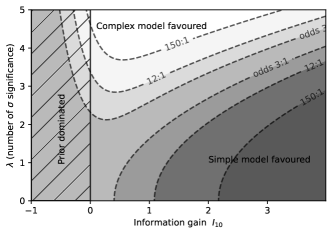
Figure 1: Posterior odds ratio for nested Gaussian models vs. (prior width/likelihood width), plotted against the ”significance” of the tension (number of ). We see that as a minimum, 3-4 tension is needed before the more complex model is favoured with odds of more than 20:1 (from Trotta, private comm.). One limitation of the Bayesian Evidence approach is that if many extra parameters are added, the uncertainty in the added prior volume may become extremely large, and the Bayes factor may be highly uncertain, see e.g. Ref. (Lin:2017ikq, ). This has prompted the investigation of other techniques, such as the Index of Inconsistency (Lin:2017ikq, ; Lin:2017bhs, ), the suspiciousness (Handley:2019pqx, ; Lemos:2019txn, ) and statistic (Joudaki:2016mvz, ; Joudaki:2020shz, ), which are not dependent on the prior. Other measures have been considered by Refs. (Raveri:2018wln, ; Seehars:2014ora, ; Adhikari:2018wnk, ; Kunz:2006mc, ; Grandis:2015qaa, ; Grandis:2016fwl, ; Nicola:2018rcd, ).
-
•
Likelihood distribution Koo:2020wro ; Koo:2021suo . This data-driven, frequentist, model validation technique that uses the method of the iterative smoothing of residuals. In other words, this method seeks to test whether the data is generated from a model, independent of how well other models fit the data. The basic procedure to validate a model on a given dataset is to start with the best-fit model to that dataset. Then the iterative smoothing method is applied to that best-fit model; that best-fit model serves as the initial guess for the iterative smoothing method. The iterative smoothing method works by, at each iteration, altering the current function such that the residuals are reduced, as in smoothed, thus improving the of the current iterated function. The likelihood distribution then calculates how much over-fitting the iterative smoothing method will perform, i.e. if the data is generated from some fiducial parameters of some model, then how much improvement in the is expected when the best-fit of the model is used as an initial guess of the iterated smoothing method. The distribution of the improvement from the iterative smoothing method over different realizations of the data is the likelihood distribution. If the improvement on the real data is outside of the likelihood distribution, then that model is invalidated, ruled out. If the improvement on the real data is within the likelihood distribution, then that model is validated.
In summary, there are many tools that have been proposed to quantify tensions, and these are used to indicate whether that new physics is needed. Quantitatively, the principled Bayesian approach is to use the Bayesian Evidence, which gives posterior odds on models, and this to some degree incorporates an element of Occam’s razor. Arguably, this is the best approach when comparing models with one or two extra parameters over CDM, but the prior-dependency of the Bayes factor may become a problem when many extra parameters are added and their prior is not easily constrained, as the Bayes factor may then be determined largely by the prior choice. There are many other instruments that may lack a principled basis, but do not suffer from this limitation. The use and interpretation of such instruments raises interesting questions, some of which are similar to the discussion of p-values elsewhere in science.222https://www.nature.com/articles/d41586-019-00874-8; https://www.nature.com/articles/d41586-019-00857-9 Are our instruments fit for purpose, and are they interpreted correctly? The alternative models considered almost always involve additional model complexity, and in circumstances where one cannot conveniently use the Bayes factor, the extent to which tools can properly penalise additional complexity (assuming we accept Occam’s view) is not always clear. Another general concern is with the complexity of the data that we collect. Our data models are inevitably simplifications and do not capture all of the astrophysics that is relevant for the real Universe. The influence of such model mis-specification on our inference is one that is rarely explored, and requires further investigation in future, whatever the statistics used.
IV The Tension
Coordinators: Simon Birrer, Adam Riess, Arman Shafieloo, and Licia Verde.
Contributors: Adriano Agnello, Eleonora Di Valentino, Celia Escamilla-Rivera, Valerio Marra, Michele Moresco, Raul Jimenez, Eoin Ó Colgáin, Tommaso Treu, Clécio R. Bom, Mikhail M. Ivanov, Leandros Perivolaropoulos, Oliver H. E. Philcox, Foteini Skara, John Blakeslee.
The 2018 legacy release from the Planck satellite Planck:2018nkj of the Cosmic Microwave Background (CMB) anisotropies, together with the latest Atacama Cosmology Telescope (ACT-DR4) ACT:2020gnv and South Pole Telescope (SPT-3G) SPT-3G:2021wgf measurements, have provided a confirmation of the standard CDM cosmological model. However, the improvement of the methods and the reduction of the uncertainties on the estimated cosmological parameters has seen the emergence of statistically significant tensions in the measurement of various quantities between the CMB data and late time cosmological model independent probes. While some proportion of these discrepancies may eventually be due to the systematic errors in the experiments, their magnitude and persistence across probes strongly hint at a possible failure in the standard cosmological scenario and the necessity for new physics.
The most statistically significant and long-standing tension is in the estimation of the Hubble constant between the CMB data, that are cosmological model dependent and are obtained assuming a vanilla CDM model, and the direct local distance ladder measurements. The Hubble constant is the present expansion rate, defined as where and .
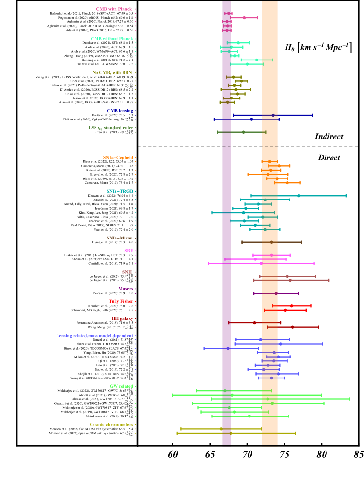
In particular, we refer to the Hubble tension as the disagreement at between the Planck collaboration Planck:2018vyg value, at 68% confidence level (CL), and the latest 2021 SH0ES collaboration (R21 Riess:2021jrx ) constraint, at 68% CL, based on the Supernovae calibrated by Cepheids. However, there are not only these two values, but actually two sets of measurements, and all of the indirect model dependent estimates at early times agree between them, such as CMB and BAO experiments, and the same happens for all of the direct late time CDM-independent measurements, such as distance ladders and strong lensing. We will see a collection of estimates in the next subsections, and a summary in the whisker plot of Fig. 2.
IV.1 Late Measurements
We consider as ”Late measurements” those that are independent of the standard CDM model. In general all of these measurements are in agreement with a higher value for the Hubble constant, and are in tension with the CMB estimate with a different statistical significance depending on the observable.
Here we find for example the best-established and empirical method of the ”distance ladder”, which allows one to measure locally, measuring the distance-redshift relation. In this case the geometry, e.g. the parallax, is used to calibrate the luminosities of specific star types which can be seen at great distances. Supernovae calibrated by Cepheids, as it has been done by the SH0ES collaboration, belong to this category. The latest SH0ES measurement gives at 68% CL Riess:2021jrx , a disagreement with the CMB one, while previous estimates include at 68% CL Riess:2020fzl , improved with the latest parallax measurements provided by ESA Gaia mission Early Data Release 3 (EDR3) gaiacollaboration2020gaia , at 68% CL Riess:2019cxk , at 68% CL Reid:2019tiq , at 68% CL Riess:2018uxu , and at 68% CL Riess:2016jrr . Finally, we have to consider also the final result of the Hubble Space Telescope Key Project, that was HST:2000azd , or the result obtained using an improved geometric distance calibration to the Large Magellanic Cloud (LMC), i.e. Freedman:2012ny .
There has been many independent works trying to re-analyze the SH0ES collaboration result in the last few years, using different formalisms, statistical methods or parts of the dataset, but there is no evidence for a drastic change of the value of the Hubble constant. We have for example the re-analysis of Ref. Cardona:2016ems using Bayesian hyper-parameters, i.e. at 68% CL, or of Ref. Camarena:2021jlr using the cosmographic expansion of the luminosity distance, i.e. at 68% CL (see Ref. Camarena:2021jlr for the - covariance) or the previous estimate Camarena:2019moy . We have also the measurement obtained by Ref. Dhawan:2017ywl using the measured near-infrared (NIR) Type Ia supernovae (SNIa), i.e. at 68% CL, or by Ref. Burns:2018ggj using a different method for standardizing SNIa light curves, i.e. at 68% CL. We have still the Hubble constant measured by Ref. Follin:2017ljs leaving the reddening laws in distant galaxies uninformed by the Milky Way, i.e. at 68% CL, or by Ref. Feeney:2017sgx using a Bayesian hierarchical model of the local distance ladder, i.e. at 68% CL. Then we have the measurement based on the Cepheids from the second Gaia data release (GDR2), that is at 68% CL Breuval:2020trd , where ZP is the GDR2 parallax zero-point. Finally, there is the re-analysis of the Cepheid calibration used to infer the local value of the from SNIa, where one does not enforce a universal color-luminosity relation to correct the near-IR Cepheid magnitudes, which gives , or , at 68% CL depending on the approach Mortsell:2021nzg , and at 68% CL in Ref. Mortsell:2021tcx .
At the same time, the impact of known and several previously neglected or unrecognized systematic effects on the center values of the SH0ES results has been constrained to be well below the level (AndersonRiess:2018, ; Anderson:2019lbz, ; Riess:2020xrj, ; Javanmardi:2021viq, ; Anderson:2021fsp, ). Interestingly, correcting reported values for such systematic effects can result in an increased value of (e.g., due to time dilation of observed variable star periods, cf. Ref. Anderson:2019lbz ), and thus, to an increased significance of the discord between the distance ladder and the early Universe-based values.
An independent determination of is based on calibration of the Type Ia supernovae (SNIa) using the Tip of the Red Giant Branch, where one finds at 68% CL Jang:2017dxn , at 68% CL Freedman:2019jwv , at 68% CL Yuan:2019npk , and the final at 68% CL Freedman:2020dne . Then we have at 68% CL Reid:2019tiq , and the estimate using velocities and TRGB distances to 33 galaxies located between the Local Group and the Virgo cluster, at 68% CL Kim:2020gai . Moreover, it is important to mention the Freedman result at 68% CL Freedman:2021ahq , or the re-analysis of Ref. Anand:2021sum that gives at 68% CL. Finally, there are the latest measurements at 68% CL of Ref. Jones:2022mvo and at 68% CL of Ref. Dhawan:2022yws .
A larger value for is preferred also by the analysis of the near-infrared HST WFC3 observations of the Mira variable red giant stars in NGC 1559, that gives at 68% CL Huang:2019yhh .
A measurement of the Hubble constant can be obtained with the Surface Brightness Fluctuations (SBF) method calibrated from Cepheids, with at 68% CL Cantiello:2018ffy from a single galaxy (the host of GW170817) at 40 Mpc and at 68% CL Khetan:2020hmh from using SBF as an intermediate rung between Cepheids and SNIa. A re-analysis of the latter performed by Ref. Blakeslee:2021rqi , improving the LMC distance, gives instead at 68% CL. Moreover, if SBF is used as another long-range indicator calibrated by Cepheids and TRGB, Ref. Blakeslee:2021rqi finds at 68% CL from a new sample of HST NIR data for 63 galaxies out to 100 Mpc.
Another possible observable to constrain is given by the Standardized Type II supernovae. Using 7 SNe II with host-galaxy distances measured from Cepheid variables or the TRGB, the Hubble constant is equal to at 68% CL deJaeger:2020zpb , while with 13 SNe II Ref. deJaeger:2022lit finds at 68% CL.
An important independent result was obtained with the Megamaser Cosmology Project, which gives an estimate by using the geometric distance measurements to megamaser-hosting galaxies, finding at 68% CL Gao:2015tqd , and at 68% CL Pesce:2020xfe , independent of distance ladders.
In addition, there are the estimates of the Hubble constant based on the Tully-Fisher Relation, i.e. the correlation between the rotation rate of spirals and their absolute luminosity used to measure the galaxy distances. Using optical and infrared calibrated Tully-Fisher Relations, the Hubble constant is equal to at 68% CL Kourkchi:2020iyz . Considering the baryonic Tully-Fisher relation (bTFR) as a new distance indicator, instead, the Hubble constant is found to be at 68% CL Schombert:2020pxm , and at 68% CL Kourkchi:2022ifq .
An estimate of can also be obtained by modeling the extragalactic background light and its role in attenuating -rays, but this is challenging and the uncertainties may be underestimated. In this case there is Ref. Dominguez:2013mfa that finds at 68% CL, the updated value at 68% CL Dominguez:2019jqc , and at 68% CL Zeng:2019mae .
The HII galaxy measurement can also act as a good distance indicator independent of SNIa to probe the background evolution of the Universe. Using 156 HII galaxy measurements, we obtain the constraint at 68% CL Wang:2016pag , which is more consistent with the value from the SH0ES Team than that from the Planck collaboration (see also FernandezArenas:2017dux )
Moreover, we have the strong lensing time delays estimates, that are not CDM model dependent but still astrophysical model dependent, because of the imperfect knowledge of the foreground and lens mass distributions. Here we have the H0LiCOW inferred values at 68% CL in 2016 Bonvin:2016crt , at 68% CL in 2018 Birrer:2018vtm , and at 68% CL in 2019 Wong:2019kwg ,333Ref. Wong:2019kwg and the follow-up paper Millon:2019slk find a descending trend of with lens redshift. This can be interpreted as an expected signature of a late-time resolution to tension in line with the explanation given in Ref. Krishnan:2020vaf (see also Ref. Krishnan:2020obg ; Dainotti:2021pqg ). Alternatively, switching to orientation on the sky, one can interpret it as a signature of an emergent dipole in Krishnan:2021dyb . based on strong gravitational lensing effects on quasar systems under standard assumptions on the radial mass density profile of the lensing galaxies. A reanalysis of H0LiCOW’s four lenses is performed in Ref. Yang:2020eoh finding at 68% CL. Under the same assumptions, the STRIDES collaboration measures from the strong lens system DES J0408-5354 at 68% CL Shajib:2019toy . Their combination (6 lenses from H0LiCOW and 1 from STRIDES, i.e. TDCOSMO) gives instead at 68% CL Millon:2019slk . Relaxing the assumptions on the mass density profile for the same sample of lenses, the TDCOSMO collaboration obtains at 68% CL Birrer:2020tax , and at 68% CL Birrer:2020tax , by combining the time-delay lenses with non time-delay lenses from SLACS (Bolton:2008xf, ), assuming they are drawn from the same parent sample.
An independent determination of has been obtained from strongly lensed quasar systems from the H0LiCOW program and Pantheon SNIa compilation using Gaussian process regression. This gives at 68% CL Liao:2019qoc , or the updated result at 68% CL using six lenses of the H0LiCOW dataset Liao:2020zko . Moreover, Ref. Qi:2020rmm finds at 68% CL, taking the derived products of H0LiCOW, and another time-delay strong lensing measurement has been obtained analysing 8 strong lensing systems in Denzel:2020zuq giving at 68% CL.
Finally, a promising probe is the angular diameter distance measurements from galaxy clusters. Using the sample consisting of 25 data points, Ref. Wang:2017fcr finds at 68% CL, or using another sample containing 38 data points at 68% CL. This measurement is very sensitive to the temperature calibration and a more conservative analysis gives at 68% CL, where errors are dominated by uncertainties of the temperature calibration Wan:2021umh , and at 68% CL Mantz:2021lcj .
When the late Universe estimates are averaged in different combinations, these values disagree between 4.5 and 6.3 with those from Planck Riess:2020sih ; Verde:2019ivm ; DiValentino:2020vnx .
IV.2 Cosmological Inferences from Modeled Galaxy Aging and BAO
In recent years, we have witnessed an increased use of reconstructions of cosmological parameters directly from data. While Gaussian Process (GP) regression Holsclaw:2010nb ; Holsclaw:2010sk ; Shafieloo:2012ht ; Seikel:2012uu is the most commonly used technique, there are a host of other approaches Crittenden:2005wj ; Crittenden:2011aa , including most recently the use of machine learning algorithms Arjona:2019fwb ; Arjona:2020kco ; Mehrabi:2021cob . The upshot of these reconstruction approaches is evident: one can reconstruct the Hubble parameter directly from cosmological data without assuming a cosmological model, at least in the traditional sense. Moreover, in the context of the Hubble constant , one can determine by simply extrapolating to . These approaches are commonly labelled ”model independent” or ”non-parametric”, since they do not make use of a traditional ”parametric” cosmological model, such as CDM, CDM, and so on.444There are some caveats to the ”model independent” moniker. One fairly obvious caveat is that reconstructions typically assume correlations, which can lead to interesting results e.g. suggestive wiggles in parameters Zhao:2017cud ; Wang:2018fng , but may not be tracking effective field theories Colgain:2021pmf . See Ref. Pogosian:2021mcs ; Raveri:2021dbu for the pronounced difference a theory prior can make. A secondary concern with GP is that the results depend on the assumed covariance matrix and there may be a tendency to underestimate errors OColgain:2021pyh (see also Ref. Dhawan:2021mel ).
One can construct directly using Cosmic Chronometers (CC) data Jimenez:2001gg ; Moresco:2012jh ; Moresco:2015cya ; Moresco:2016mzx ; Moresco:2022phi , before extrapolating to , as explained above.555The novelty and added value of the CC with respect to other cosmological probes is that it can provide a direct estimate of the Hubble parameter without any cosmological assumption (beyond that of an FLRW metric). From this point of view, the strength of this method is its (cosmological) model independence: no assumption is made about the functional form of the expansion history or about spatial geometry; it only assumes homogeneity and isotropy, and a metric theory of gravity. Constraints obtained with this method, therefore, can be used to constrain a plethora of cosmological models Jimenez:2019cll . The advantage of the cosmic chronometer method is that it infers directly from the differential age evolution of the most massive and passively evolving galaxies, selected to minimize any possible contamination by star-forming objects. A current comprehensive review on this cosmological probe is provided in Ref. Moresco:2022phi , and a summary discussed in Sect. VI.4. Current datasets constrain to and , respectively for a generic open CDM and for a flat CDM cosmology Moresco:2022phi . Moreover, CC observations are also ideal to derive from GP extrapolations, since not only is GP model agnostic, at least subject to some caveats, but the CC method itself is fully cosmological model independent.
Using 30 CC data points, the Hubble constant is constrained to at 68% CL Wang:2016iij . Analysing 31 data measured by the cosmic chronometers technique and 5 data by BAO observations, the Hubble constant is equal to at 68% CL Yu:2017iju . Given recent criticism Kjerrgren:2021zuo , some caveat has to be taken when considering the preliminary analysis obtained with CC, while the treatment of both statistical and systematic errors have been fully studied and taken into account in subsequent analyses Moresco:2018xdr ; Moresco:2020fbm ; Borghi:2021rft However, at , any discrepancy with the SH0ES determination Riess:2020fzl is negligible, despite (systematic) errors being possibly underestimated.
An interesting extension of this analysis, including the SNIa data from the Pantheon compilation and the Hubble Space Telescope (HST) CANDELS and CLASH Multy-Cycle Treasury (MCT) programs, gives instead at 68% CL Gomez-Valent:2018hwc , and when use is made of the Weighted Polynomial Regression technique Gomez-Valent:2018hwc . Observe that the inclusion of SNIa has dramatically reduced the errors and the discrepancy with the SH0ES result Riess:2020fzl becomes and , respectively. A novel feature of this analysis is that since SNIa require a calibrator to determine , CC data are being used to calibrate SNIa in an iterative procedure Gomez-Valent:2018hwc . That being said, a discrepancy of between two a priori ”model independent” determinations, one local () and one making use of GP, is an obvious problem if one neglects i) the tendency of GP to underestimate errors and ii) CC data may not have properly propagated some systematic uncertainties.
Through an extension of the standard GP formalism, and utilising joint low-redshift expansion rate data from SNIa, BAO and CC data, the Hubble constant is found to be at 68% CL Haridasu:2018gqm , in full agreement with Gomez-Valent:2018hwc . This marks another interesting result, since an effort has been made to better account for systematic uncertainties, which improves on earlier results. Observe that the inclusion of systematic uncertainties reduces another alarming ”model independent” discrepancy with SH0ES to a much more manageable . This underscores the importance of systematic uncertainties, especially in the context of CC data as currently addressed in Ref. Moresco:2020fbm . Making use of the same combination of data, i.e. SNIa+BAO+CC, while relying only on few seminal assumptions at the basis of the distance duality relation and using a combination of uncalibrated geometrical data, the authors of Ref. Renzi:2020fnx find , showing the possibility of measuring at the percentage level without assuming a cosmological model. This determination, being midway between SH0ES and Planck is consistent with both. Whereas current data do not allow for a complete resolution of the Hubble tension, this method hints at a twofold reconciliation for the values of from SH0ES, TRGB Freedman:2019jwv ; Freedman:2020dne and Planck Planck:2018vyg . An adjustment in the calibration of the SNIa, i.e. setting , lower than SH0ES calibration, bringing local measurements in agreement; and a mild deviation from CDM in the expansion history at intermediate redshift to bring the latter in agreement with the early time measurement of Planck.
Interestingly, the inferences from GP are not restricted below . In particular, one can remove SNIa and replace standard BAO with a combination of transversal BAO scale , with BBN and CC, to arrive at the value at 68% CL Nunes:2020uex , which remarkably is completely consistent with the latest SH0ES determination.
Finally, a combined analysis of SNIa, CC, BAO, and H0LiCOW lenses gives at 68% CL Bonilla:2020wbn . Once again, this estimation is in agreement with SH0ES and H0LiCOW collaborations within 68% CL. This may not be so surprising given that H0LiCOW Wong:2019kwg prefers a value for the Hubble constant , but observe that all data are still cosmological in nature.
Clearly, GP regression reconstructions of , and by extrapolation , can lead to different results. In particular, the central values range from Gomez-Valent:2018hwc , consistent with Planck Planck:2018vyg , all the way to , consistent with SH0ES Riess:2020fzl . Of course, the final outcome depends on the data, but it is worth emphasising that all the observational data are purely cosmological in nature, so the determinations are independent of the local () determinations outlined in Sec. IV.1. For this reason, comparison is meaningful. Throughout CC data is playing a special role in calibrating SNIa and BAO, so it is imperative to unlock the potential in CC by fully accounting for systematic uncertainties and adding new data points. In particular, it will be fundamental to improve and validate galaxy stellar population modeling - which currently represents the main source of systematic uncertainty Moresco:2020fbm - and to increase the CC statistics with upcoming galaxy spectroscopic surveys. With these improvements, one distinct possibility is that data reconstructions may converge to a Planck value Gomez-Valent:2018hwc ; Haridasu:2018gqm . If they do, given the model independent setup, then either higher local determinations are wrong, the cosmological data are wrong, or the Universe is not FLRW, see Sec. VII.8 and Sec. VIII.6.
IV.3 Gravitational Waves Standard Sirens
It is possible to have Hubble constant measurements from the GW standard sirens: modelling early data on the GRB170817 jet Ref. Guidorzi:2017ogy gives at 68% CL; late-time GRB170817 jet superluminal motion gives at 68% CL Hotokezaka:2018dfi ; from the dark siren GW170814 BBH merger Ref. DES:2019ccw finds at 68% CL; from GW170817 and 4BBH from O1 and O2 one obtaines at 68% CL LIGOScientific:2018hze ; finally, from GW190814 and GW170817 one finds at 68% CL LIGOScientific:2020zkf . The most recent result on this observable reported by the LIGO-Virgo-KAGRA Collaboration yields LIGOScientific:2021aug . This was obtained using a method that constrains the source population properties of BBHs without galaxy catalogue, but still combines with GW170817 Bright Siren (without GW170817 the result is ). Other recent dark siren results from Ref. Palmese:2021mjm , using only catalogues from Legacy Survey and no galaxy weighting, presents the value when combined with GW170817, and without. Finally, we have the latest at 68% CL from Ref. Mukherjee:2022afz cross-correlating dark-sirens and galaxies.
We will discuss the expected improvement in the future using GW in Sec. IX.1.7.
IV.4 Early Measurements
We consider as ”Early measurements” those based on the accuracy of a number of assumptions, such as the model used to describe the evolution of the Universe, i.e. the standard CDM scenario, the properties of neutrinos or the Dark Energy (a cosmological constant), the inflationary epoch and its predictions, the number of relativistic particles, the Dark Matter properties, etc. For this reason the Hubble constant tension can be the indication of a failure of the assumed vanilla CDM scenario, particularly the form it takes in the pre-recombination Universe. In general all of these measurements are in agreement with a lower value for the Hubble constant.
As we can see in Fig. 2, there are a variety of CMB probes preferring smaller values of . For example, we can see the satellite experiments, such as the Wilkinson Microwave Anisotropy Probe (WMAP9) WMAP:2012nax that assumes the CDM model, gives a value for the Hubble constant at 68% CL in its nine-year data release. Moreover, the Planck 2018 release Planck:2018vyg predicts at 68% CL or in combination with the CMB lensing Planck:2018vyg , i.e. the four-point correlation function or trispectrum analysis, that estimates at 68% CL. However, in perfect agreement there are the ground based telescopes, such as the ACT-DR4 estimate at 68% CL ACT:2020gnv . Alternatively, SPT-3G SPT-3G:2021eoc returns the value of at 68% CL. Finally, they can be combined together so that ACT+WMAP finds at 68% CL ACT:2020gnv .
Yet, also on the low side, we have combinations of complementary probes, such as Baryon Acoustic Oscillation (BAO) data Beutler:2011hx ; Ross:2014qpa ; Alam:2016hwk , Big Bang Nucleosynthesis (BBN) measurements of the primordial deuterium Cooke:2017cwo , weak lensing and cosmic shear measurements from the Dark Energy Survey DES:2021wwk . For example, the final combination of the BAO measurements from galaxies, quasars, and Lyman- forest (Ly-) from BOSS and eBOSS prefers at 68% CL for inverse distance ladder analysis involving a BBN prior on the physical density of the baryons eBOSS:2020yzd .
Galaxy power spectra can be used to constrain indirectly the Hubble parameter, via the indirect effect of on the shape of the matter transfer function, in principle without requiring a calibration of the sound-horizon from the CMB as in inverse-distance-ladder approaches (see Sec. VI.2), but using effectively the matter radiation equality horizon calibrated from the CMB, and thus using a different but closely related inverse-distance-ladder approach. A reanalysis of the Baryon Oscillation Spectroscopic Survey (BOSS) data on the full-shape (FS) of the anisotropic galaxy power spectrum gives at 68% CL Ivanov:2019pdj when the BBN prior on is used, whereas a similar analysis with the baryon-to-dark matter density ratio fixed to the Planck baseline CDM best-fit value gives at 68% CL DAmico:2019fhj . Adding the post-reconstructed BAO signal to the FS + BBN data gives at 68% CL Philcox:2020vvt (fixing the spectral slope ). This measurement was recently updated by adding the information from the power spectrum of the eBOSS emission line galaxies Ivanov:2021zmi and the BOSS DR12 bispectrum Ivanov:2021haa ; Ivanov:2021kcd ; Philcox:2021kcw , yielding and , respectively. Similar results were obtained by other groups, in particular from the anisotropic BOSS power spectrum combined with BAO and BBN measurements (Chen:2021wdi, ), or using the galaxy correlation function, BBN priors and BAO measurements from BOSS and eBOSS (Zhang:2021yna, ). By analyzing the BOSS DR12 full-shape data combined with a prior on from the Pantheon Supernovae, is found at 68% CL Philcox:2020xbv ; Farren:2021grl .
These measurements work within the CDM model and Standard Model for the early Universe, to set the power spectrum, with pros and cons as discussed in Brieden:2021edu ; Brieden:2021cfg where it is shown that without assuming standard early time physics and a CDM model the constraint likely gets significantly weakened. If the common fitting formulae of Eisensten & Hu (1998) are used, as done e.g. for the 6dFGS (section 5.2 of Beutler:2011hx, ), only a limited range for the sound horizon is allowed. Therefore, the choice of CDM+SM already sets the range of possible values to even when purely angular measurements of from BAO are used. A reappraisal of the BAO measurement of with different constraints on yielded (BAO +SN +DES +CMBlensing), without constraints on from BBN, with a difference of between measurements using CMB lensing power spectra from SPTPol or Planck Pogosian:2020ded . Statistically consistent, albeit more uncertain results can also be obtained from CMB lensing alone, (Baxter:2020qlr, ). Work by the DES-y1 combined with BAO and BBN and obtained at 68% CL DES:2017txv . This measurement was carried out within CDM+SM ( fixed to ) and used the 6dFGS BAO inference, and so it indirectly anchored It also adopted a compromise BBN estimate so that it would not be in immediate tension with Planck, which however would require a model with free Cooke:2017cwo .
IV.5 Supernovae Absolute Magnitude
In many of the papers discussing the extended cosmology resolution to the Hubble tension, the distance ladder measurements of are incorporated into the analysis as a Gaussian likelihood. Recently several works Camarena:2019moy ; Benevento:2020fev ; Camarena:2021jlr ; Efstathiou:2021ocp ; Greene:2021shv ; Cai:2021weh ; Benisty:2022psx warned against this practice due to possible caveat on extremely late Universe transitional models. The reason is that local late Universe measurements of depend on observations of astrophysical objects that extend into the Hubble flow, for example the SH0ES Riess:2016jrr results that have been most frequently quoted uses Pantheon supernovae sample in the redshift range . Hence the distance ladder actually calibrates the absolute magnitude of the supernovae sample that includes higher redshifts objects. If a model predicts a higher Hubble constant to be achieved by extremely late transitional effect at , like the example of red curve in Fig. 1 of Ref. Benevento:2020fev or the hockey-stick dark energy of Ref. Camarena:2021jlr , it is not actually resolving the Hubble tension. Ref. Raveri:2019gdp ; Camarena:2019moy give the simplest method to correctly combine the distance ladder measurement of :
| (1) |
i.e. to include the distance ladder measurement as the supernovae absolute magnitude prior. It is possible to marginalize analytically Eq. (1), similarly to the analytical marginalization that is performed when a flat prior on is assumed, see Section 4.6 of Ref. Camarena:2021jlr for details.
This detail should be especially taken care of for extended cosmological models which deviate from CDM phenomenology at late time (i.e. at low redshift). However, note that the consequence is not as severe as implied by Ref. Efstathiou:2021ocp if the transition is not restrained to . The main point of the discussion above is that the measured at late time is not exactly the value at , thus should be related to the supernovae absolute magnitude calibration at the same range of low redshifts. This means models that hide all the new physics at such low redshifts, which are irrelevant to the Hubble flow measurements, are naturally off the mark. For example, consider the red curve in Fig. 1 of Ref. Benevento:2020fev . If a model has no drastic jump in the Hubble constant at , but a gradual change throughout several redshifts, the low redshift Hubble measurement could still be a reasonable anchor of current time , and should be equivalent to Eq. (1).
Besides the previous reasons, Eq. (1) is recommended for any future analysis using distance ladder combined with supernovae samples because it avoids adopting an unnecessary cosmographic expansion: when performing cosmological inference one should use the luminosity distance of the cosmological model that is being tested. Furthermore, Eq. (1) avoids double counting low-redshift supernovae belonging to the sample that was used to perform cosmography in order to obtain the constraint.666The up-to-date prior on is maintained at github.com/valerio-marra/CalPriorSNIa and has been implemented in Monte Python 3.5. Recently, the SH0ES and Pantheon+ teams have released the SH0ES Cepheid host-distance likelihood,777pantheonplussh0es.github.io which allows for the optimal inclusion of the local calibration of the supernova absolute magnitude in the cosmological analysis of a given theoretical model.
IV.6 Distance Ladder Systematics
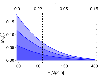
For the sake of completeness, this subsection summarizes the outstanding sources of uncertainties in the SNIa distance ladder. The determination of the local Hubble constant is affected by the large-scale structure around us. Considering a spherical inhomogeneity, one expects that an adiabatic perturbation in density causes a perturbation in the expansion rate given by:
| (2) |
where is the present-day growth function for the concordance CDM model. Fig. 3 shows the expectation for the standard model: the effect of the local structure quickly decreases by considering larger scales. This is the motivation for placing a limiting lower redshift when fitting the supernova data in order to obtain . The SH0ES collaboration adopts (Riess:2020xrj, ), for which estimates based on theoretical computations (see Ref. Camarena:2018nbr and references therein) and numerical simulations (see Ref. Odderskov:2017ivg and references therein) suggest that cosmic variance on amounts at 0.5–1%. It is worth remarking that the SH0ES collaboration tries to correct for this systematic effect by correcting the velocity field via local cosmic flow maps. TRGB estimates adopt instead the redshift range (Freedman:2021ahq, ). In this case one expects a larger cosmic variance of about 2%.
Finally, one residual contribution to systematic uncertainties, in determining both and is the uncertainty in the product from the combination of BAO and Supernovae in the ”cosmological” redshift range. Recently, the Pantheon collaboration has re-analyzed the calibration used for the photometry of the SNIa sample, including the calibration used to obtain the SH0ES results Brout:2021mpj ; Scolnic:2021amr . The contribution to the Hubble constant from the systematic SN calibration is smaller than , so that the tension cannot be attributed to this type of systematics.
V The Tension
Coordinators: Marika Asgari, Hendrik Hildebrandt, and Shahab Joudaki.
Contributors: Erminia Calabrese, Eleonora Di Valentino, Dominique Eckert, Mustapha Ishak, Mikhail M. Ivanov, Leandros Perivolaropoulos, Oliver H. E. Philcox, Foteini Skara.
Recent observations of probes of the large-scale structure have allowed us to constrain the strength with which matter is clustered in the Universe. These constraints on the strength of matter clustering differ from that inferred by probes of the early Universe. In particular, the primary anisotropies of the cosmic microwave background (CMB) as measured by the Planck satellite exhibit a tension in the matter clustering strength at the level of when compared to lower redshift probes such as weak gravitational lensing and galaxy clustering (e.g. Asgari:2019fkq ; Asgari:2020wuj ; Joudaki:2019pmv ; DES:2021wwk ; DES:2021bvc ; DES:2021vln ; KiDS:2021opn ; Joudaki:2016kym ; Heymans:2020gsg ; Hildebrandt:2018yau ; DES:2020ahh ; Macaulay:2013swa ; Skara:2019usd ; Kazantzidis:2019dvk ; Joudaki:2016mvz ; Bull:2015stt ; Kazantzidis:2018rnb ; Nesseris:2017vor ; Philcox:2021kcw ).
This tension is often quantified using the parameter, which modulates the amplitude of the weak lensing measurements. The parameter is closely related to measured by redshift space distortions (RSD) Li:2016bis ; Gil-Marin:2016wya , where approximates the growth rate in GR as a function of the matter density parameter, , at redshift . The lower redshift probes, as seen in Fig. 4, generally prefer a lower value of compared to the high redshift CMB estimates. Measuring is model dependent and in all cases here the underlying model is the standard flat CDM model. This model provides a good fit to the data from all probes, but predicts a lower level of structure formation compared to what is expected from the CMB observations.
The high redshift data from Planck TT,TE,EE+lowE finds . Combining this data with secondary CMB anisotropies, in the form of CMB lensing, serves to tighten the constraint to . Constraints from CMB lensing alone are fully consistent with both high and other low redshift measurements as seen in Fig. 4. Combining the high- data from ACT with the low- measurements of WMAP yields larger errors on ACT:2020gnv , but is consistent with the Planck results. In the following sections, we briefly describe the analyses and data used in Fig. 4 and moreover discuss the possible systematic effects associated with each probe.
In reporting parameter estimates and constraints, we note that there might be differences in the choices that enter each analysis. For instance, a statistical property of the marginal distribution might be chosen, such as its mean or mode together with the asymmetric region around them or the standard deviation of the sampled points. By contrast, in some analyses, the statistics relevant to the full posterior distribution have been adopted, such as the maximum a posteriori point or the best fitting values and their associated errors. These choices can impact the estimated values of the parameters, in particular when the posterior distributions are significantly non-Gaussian or when the parameter estimates are prior dominated (see e.g. Ref. Joachimi:2020abi ). For simplicity, we will use the nominal values reported in each analysis, but caution the reader that the methodology used may differ from case to case (see Sec. III for a more detailed discussion).
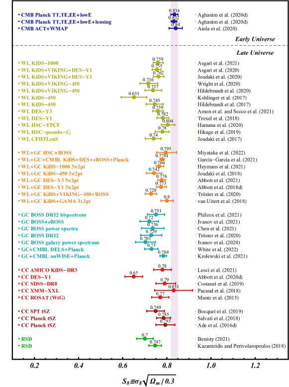
V.1 Weak Gravitational Lensing
The images of distant galaxies are gravitationally lensed by the intervening matter. On cosmological scales we use this effect to analyse and understand the large scale structures (LSS) in the Universe. The gravitational lensing effect of the LSS only slightly distorts the shapes of these galaxies (weak lensing). The two main strands of weak lensing that we focus on in this section are cosmic shear, the study of correlations between the shapes of pairs of galaxies, and galaxy-galaxy lensing, the study of the correlation between the position of foreground galaxies and background galaxy shapes. In addition, galaxy cluster abundance measurements (cluster counts, CC) also utilise gravitational lensing to estimate cluster masses. This will be covered in Sec. V.5.
Using cosmic shear we can probe the LSS more directly compared to galaxy-galaxy lensing, where we need to make assumptions about the connection between galaxies and the underlying matter distribution. In addition, cosmic shear studies provide tighter constraints on and can be used as an independent probe. In Sec. V.4, we discuss analyses that use galaxy-galaxy lensing in combination with other probes of the large scale structure, as they do not currently provide independent competitive constraints on cosmological parameters.
The tension in between weak gravitational lensing data and Planck CMB measurements was first seen when the cosmic shear analysis of CFHTLenS (Canada France Hawaii Lensing Survey, Heymans:2013fya, ) was compared to the first Planck data release (Planck:2013win, ). Back then, the tension was still mild at the level of . Subsequent analysis of the CFHTLenS data with improved methodology Joudaki:2016mvz validated these initial observations. This mild tension motivated the weak lensing community to obscure their data by blinding the team to the constraints on cosmological parameters and only unblinding once the analysis has been finalized. The first blinded analysis of this kind was performed by the Kilo Degree Survey on their first 450 square degrees of data (KiDS-450: Kuijken:2015vca, ; FenechConti:2016oun, ; Hildebrandt:2016iqg, ), which found a lower value of compared to the Planck 2015 constraints Planck:2015bpv . Cosmic shear analysis has seen significant improvements in the recent years and therefore we limit ourselves to results published in the last 5 years (since 2017).
All published results in the last 5 years have found values that are lower than the early Universe estimates. The first year data from the Dark Energy Survey (DES-Y1, DES:2017qwj, ) and Hyper Suprime Cam (HSC HSC:2018mrq, ; Hamana:2019etx, ) found slightly higher but consistent values with the KiDS-450 results. Subsequent analysis of KiDS included photometric data from VIKING which reduced the redshift errors and outlier fractions. The analyses of KiDS-450 + VIKING (KV450, Hildebrandt:2018yau, ; Wright:2020ppw, ) found consistently low results. The combination of DES-Y1 and KV450 data were analysed in Refs. Joudaki:2019pmv ; Asgari:2019fkq , finding tighter constraints in agreement with previous results. The latest cosmic shear analysis of KiDS (KiDS-1000, Asgari:2020wuj, ) and DES (DES-Y3, DES:2021bvc, ; DES:2021vln, ) show the same trend with better precision. Comparing their values with the fiducial Planck analysis, both surveys find values that are smaller.888Note that the tension level changes depending on the assumed method, see Sec. III for details.
V.2 Weak Lensing Systematics
Low-redshift measurements of large-scale structure evolution require sophisticated analysis pipelines to correct for a large number of known systematic effects. Here, we discuss the most prominent systematic uncertainties affecting the weak lensing measurements.
V.2.1 Shape Measurements
The basic observable in any weak gravitational lensing measurement is the ellipticity of a galaxy. The measured ellipticity is a combination of the intrinsic galaxy ellipticity and the shear effect of gravitational lensing. In the weak lensing regime the small shear is completely dominated by the large intrinsic ellipticity making it necessary to average over many galaxies. The idea behind this is that galaxies are intrinsically randomly oriented on the sky and the intrinsic ellipticities average to zero leaving only the shear (but see intrinsic alignments below). Under the assumption of random intrinsic orientation, a galaxy ellipticity is an unbiased but extremely noisy estimator of the shear.
In cosmic shear, pairs of galaxies are analyzed for coherent shear contributions to their ellipticities as a function of their distance. This typically involves many millions and soon billions of faint galaxy images. In practice, one has to estimate the ellipticities of these very large samples of galaxies from fuzzy, noisy images that make up a few pixels on a detector each. With weak lensing being a statistical measurement, it is not crucially important to estimate a highly accurate ellipticity measurement for every single galaxy. Rather it is important to control the average bias in the shear estimates to very low values. For current Stage-III surveys such as KiDS, DES, and HSC, biases in the shear need to be controlled to a level of , with future Stage-IV experiments requiring almost an order of magnitude better systematics control EUCLID:2011zbd ; LSSTDarkEnergyScience:2018jkl .
Several effects make this a very delicate problem. The atmosphere (in case of ground-based observations) and the telescope and camera optics introduce distortions that are significantly larger than typical shear values. These have to be corrected to high accuracy using PSF (point-spread-function) information from stars before the galaxy-based shear estimates can be used in cosmological measurements Kaiser:1994jb . In the low signal-to-noise ratio regime, the measurements further suffer from noise bias that needs to be corrected Melchior:2012un . Depending on the actual algorithm, other biases like model bias can play a role Voigt:2009mj ; Miller:2012am . Furthermore, any sample selection (e.g. through source detection Hoekstra:2020zyl and tomographic binning via photometric redshifts) can introduce further biases. The electronics of CCDs also play a crucial role and must be understood at a deep level Rhodes:2010yg ; Gruen:2015pcc ; Boone:2018iqq ; coulton18 ; Massey:2009wv .
In order to reach the required accuracy, it is usually necessary to simulate the whole process with a dedicated suite of image simulations, often based on or informed by high-resolution HST (Hubble Space Telescope) observations Rowe:2014cza ; FenechConti:2016oun ; Kannawadi:2018moi ; Hoekstra:2016kaj ; DES:2020lsz ; Mandelbaum:2017ctf ; Bruderer:2015bsa ; Li:2021mvq . Only in this way can the crucial multiplicative bias, which describes the systematic over-/under-estimation of shear values, be calibrated. The community has engaged in several blind challenges over the past two decades to objectively determine the remaining multiplicative biases in weak lensing measurements Heymans:2005rv ; Massey:2006ha ; Bridle:2009gg ; Kitching:2012rt ; Mandelbaum:2014fta . State-of-the-art algorithms suppress this bias to very small levels at runtime Huff:2017qxu ; Sheldon:2017szh ; Sheldon:2019uxq ; Kannawadi:2020rok ; Hoekstra:2021plm . But it is really the robustness to small differences between the image simulations that are ultimately used for calibration and the real Universe that determines the quality of a shape measurement method.
A residual bias in the shear estimates scales almost linearly with . Hence, the community has put a lot of effort over the past two decades (arguably more effort than into any other weak lensing systematic) into controlling these biases to the percent level in current surveys and is working towards an even better control for stage-IV experiments. As such, the current tension in between cosmic shear measurements and Planck is most probably not due to uncontrolled systematics in the shear measurement.
V.2.2 Photometric Redshifts
The cosmic shear signal measured from wide-field imaging surveys scales strongly with redshift VanWaerbeke:2006qt . The higher the redshift of the sources, the stronger the signal due to the increased light path and integrated deflection and distortion of the light-bundles along their way. As the measurement is inherently statistical, averaging the signal from millions of source galaxies, it is the ensemble redshift distribution of all sources that needs to be known to high accuracy in order to obtain unbiased model predictions for the cosmic shear signal. This accuracy is traditionally summarised in the uncertainty of the mean redshift of all sources, as the integrated nature of the cosmic shear effect means that higher-order moments of the redshift distribution are less important for accurate predictions. In order to allow measurements at different cosmic epochs and increase the constraining power for various cosmological parameters, the galaxy source sample is typically split up into tomographic redshift bins via individual photometric redshift estimates.
Both tasks, determining precise individual galaxy redshifts for the tomographic binning as well as estimating accurate redshift distribution(s) for the ensemble(s), require photometric techniques because of the large number of faint sources that makes spectroscopic measurements of complete weak lensing source samples infeasible. Typically, a subset of sources is observed spectroscopically and can be used to validate, train, and calibrate the photometrically determined redshifts and redshift distributions.
The individual photometric redshifts used for binning the galaxies along the line-of-sight are unimportant for the accuracy of measurements from cosmic shear. Rather, their precision influences the signal-to-noise ratio of those measurements and the constraining power of a survey. Thus, these individual photometric redshifts cannot cause a bias in and will not be discussed in the following. By contrast, the accuracy of the redshift distribution directly impacts the accuracy of cosmological parameter estimates Huterer:2005ez . Any bias in the mean redshifts of the tomographic bins causes a bias in .999This is strictly only true in the non-tomographic case or in case of coherent biases of all tomographic bins. Incoherent redshift biases of different tomographic bins can cause e.g. spurious IA signals. If the mean redshift estimate is biased high the estimate will be biased low and vice versa. In practice, one marginalises over the uncertainty in the mean redshifts.
For contemporary Stage-III weak lensing surveys, the requirement on the accuracy of the mean redshifts of the tomographic bins is on the order of 0.01 Hildebrandt:2016iqg ; Tanaka:2017lit ; DES:2017ndt . This is necessary for the marginalisation over the redshift uncertainty to not compromise the statistical power of the surveys. Stage-IV surveys such as Euclid and LSST will require a calibration that is more accurate by a factor of to reach that goal EUCLID:2011zbd ; LSSTDarkEnergyScience:2018jkl . The importance of this redshift calibration has triggered a lot of work that aims at minimising biases in the determination of the source redshift distributions by different techniques that rely on different types of (typically spectroscopic) calibration samples. Broadly, these can be categorised as either colour-based or position-based techniques.
The colour-based techniques typically employ a deep spectroscopic calibration/reference sample that is as representative of the sources as possible. Any mismatch in redshift between the source and the reference samples needs to be removed before a reliable redshift distribution can be estimated. This is usually done by some re-weighting technique that takes the relative densities of both samples in high-dimensional colour/magnitude space into account Lima:2008kn ; Gruen:2016jmj ; DES:2020lea . Early attempts used -nearest-neighbour counting to estimate these densities whereas most contemporary surveys have employed self-organising maps Masters:2015asa ; DES:2019bxr ; Wright:2019fwm ; DES:2020ebm ; Wright:2020ppw ; Nishizawa:2020gac . This latter technique has the advantage of easy visualisation and allows culling of the source sample to remove parts of colour space that are not covered by the spectroscopic reference sample. Covering the colour/magnitude space of future stage-IV weak lensing experiments with deep spectroscopic observations is a huge task. Dedicated spectroscopic surveys on the biggest available optical and near-infrared telescopes are being conducted to secure this essential calibration data Newman:2013cac ; Masters:2017fho ; Masters:2019ptz ; Euclid:2021ueh ; Euclid:2020xbm .
Complementary to the colour-based redshift calibration are techniques that exploit the fact that galaxies are clustered Newman:2008mb ; Hildebrandt:2016iqg ; Hildebrandt:2020rno ; Morrison:2016stl ; DES:2020rlj ; vandenBusch:2020lur . Using a wide-area spectroscopic reference sample that covers the whole redshift range of interest, the redshift distributions of the weak lensing source sample can be determined via an angular cross-correlation approach. The amplitude of the angular cross-correlation between thin redshift slices of the reference sample and the unknown target sample (e.g. tomographic bins) is directly related to the target sample’s redshift distribution. The great advantage of this technique is that the reference samples does not have to be representative of the target sample, e.g. one can use a bright reference sample to estimate the redshift distribution of a faint target sample since both samples cluster with each other. Correcting for the redshift evolution of galaxy bias in both samples is crucial because it is degenerate with the amplitude of the redshift distribution. This can be done via angular auto-correlation measurements for the reference sample and consistency checks for the target sample.
Both techniques of redshift calibration have been thoroughly tested against each other and on increasingly complex simulations over the past few years. So far, there is no indication that the tension is caused by a bias in the redshift calibration. A substantial amount of work still needs to be carried out to get those techniques ready for Stage-IV experiments, possibly combining colour and position information Alarcon:2019jyt ; Sanchez:2018wuh ; LSSTDarkEnergyScience:2021ozf , but the current results from weak lensing seem quite robust in the light of these tests.
V.2.3 Intrinsic Galaxy Alignments
The intrinsic alignment (IA) of galaxies constitutes one of the most significant sources of systematic uncertainties in weak lensing (e.g. Refs. Hirata:2004gc ; Troxel:2014dba ; Heymans:2013fya ; Mandelbaum:2017jpr ; Bridle:2007ft ; Heymans:2003pz ; Joudaki:2016mvz ; Vlah:2019byq ; Leonard:2018aow ; Blazek:2011xq ; Blazek:2015lfa ; Krause:2015jqa ; Kirk:2010zk ; Kirk:2011aw ; Blazek:2017wbz ; Joachimi:2013una ; Chisari:2015qga ; Johnston:2018nfi ; Fortuna:2020vsz ; Samuroff:2020gpm ). It was shown in Refs. Bridle:2007ft ; Heymans:2003pz that if intrinsic alignments are ignored in Stage-IV weak lensing analyses (such as Euclid and LSST), the equation of state of dark energy will be biased by up to and the amplitude of matter fluctuations will be biased by up to . Intrinsic alignments of galaxies refer to correlations between galaxies that arise due to the tidal gravitational field where these galaxies formed. These intrinsic alignments produce a spurious signal that contaminates the genuine lensing signal and any cosmological information inferred from it. Interestingly, there are two types of intrinsic alignments that affect lensing on large scales. The first is due to relatively close galaxies being radially aligned by the same dark matter structure, known as the ”intrinsic shear – intrinsic shear”, or II, correlation. The second type is due to the fact that a dark matter structure aligns radially neighbouring galaxies and at the same time tangentially shears the background galaxy images, thus creating an anti-correlation between the two known as the ”gravitational shear – intrinsic shear” correlation, or GI, term. See reviews in Refs. Troxel:2014dba ; Kiessling:2015sma ; Kirk:2015nma and references therein.
After two decades of developing methods to mitigate the effects of intrinsic alignment contamination to the lensing signal in photometric galaxy surveys, two methods have emerged as being the most efficient at addressing the problem. One is the common marginalization method where an IA model is assumed and its parameters are constrained along with the cosmological parameters (see e.g. Ref. Joudaki:2017zdt ). The other method is the self-calibration method that is based on calculating additional correlations from the same lensing survey by taking into account the positions of the lens with respect to the sources within the same bin and then using a scaling relation that relates such a correlation to cross-correlations between bins. This method strongly complements the marginalization method as it does not need to assume an IA model and is able to separate the IA signal from the lensing signal (see e.g. Ref. Troxel:2011za ). It was shown in Ref. Yao:2017dnt that not correcting for intrinsic alignments can shift cosmological parameters as determined from weak lensing and that correlations between the IA amplitude and other parameters are present. Similarly, it was shown earlier in Ref. Dossett:2015nda that the IA amplitude has some correlation with but that it is not significant enough to explain the tension. This was confirmed in Ref. Yao:2017dnt . It is fair to assert that while intrinsic alignments need to be corrected for in an era or precision cosmology, these cannot be responsible for a significant tension in between lensing and the CMB.
V.2.4 Matter Power Spectrum Including Baryonic Feedback
The matter power spectrum can be accurately obtained on linear scales via Boltzmann codes such as CAMB Lewis:1999bs and CLASS Blas:2011rf . In order to obtain the matter power spectrum on nonlinear scales, numerical simulations need to be carried out at multiple cosmologies spanning the full parameter space of interest (see e.g. Refs. Lawrence:2009uk ; Schaye:2009bt ; Heitmann:2015xma ; McCarthy:2016mry ; Euclid:2018mlb ; Euclid:2020rfv ). An emulator for the simulations or a fitting function calibrated to the simulations can then be created. Examples of emulators include Cosmic Emu Lawrence:2009uk ; Heitmann:2013bra ; Lawrence:2017ost and Euclid Emulator Euclid:2018mlb ; Euclid:2020rfv , while the two most popular fitting functions are Halofit Smith:2002dz ; Takahashi:2012em and HMCODE Mead:2015yca ; Mead:2016zqy ; Mead:2020vgs . On nonlinear scales, the impact of baryonic processes such as radiative cooling, star formation, and feedback from supernovae and active galactic nuclei (AGN) also needs to be taken into account (see e.g. Ref. Chisari:2019tus for a review). A particular benefit of HMCODE is that, in addition to calibrating against dark matter simulations, it accounts for these baryonic effects by calibrating against hydrodynamical simulations (originally to the OverWhelmingly Large Simulation, or OWLS, suite Schaye:2009bt ; vanDaalen:2011xb ; Brun:2013yva and most recently to the BAryons and HAloes of MAssive Systems, or BAHAMAS, suite McCarthy:2016mry ).
The uncertainties in the dark matter simulations and emulators of the matter power spectrum are at the few-percent level down to scales of Lawrence:2017ost ; Euclid:2020rfv . These uncertainties grow to 5%-10% for the fitting functions for the same highly nonlinear scales Takahashi:2012em ; Mead:2020vgs . Meanwhile, the uncertainties in the hydrodynamical simulations boil down to the choices that need to be made in regards to the stellar and hot gas content. The uncertainty in the simulations themselves are at the few-percent level (see e.g. Refs. vanDaalen:2011xb ; Chisari:2018prw ), but the impact of baryonic feedback on the matter power spectrum differs substantially between different simulations (suppressing the power between – for scales in the range of few and ) due in particular to their different choices for the sub-grid model, resolution, and calibration strategy Chisari:2018prw ; Huang:2018wpy ; Chisari:2019tus . Further work is therefore needed to capture the impact of baryonic feedback on the nonlinear matter power spectrum to the precision needed for next-generation cosmological surveys. While the KiDS Hildebrandt:2016iqg ; Hildebrandt:2018yau ; Asgari:2020wuj ; Joudaki:2016kym ; Kohlinger:2017sxk ; Joudaki:2017zdt ; vanUitert:2017ieu ; Heymans:2020gsg and HSC HSC:2018mrq ; Hamana:2019etx analyses have attempted to account for the uncertainty in the matter power spectrum due to baryonic feedback by introducing one or more nuisance parameters, the fiducial approach in the DES analyses DES:2017qwj ; DES:2021vln ; DES:2021bvc ; DES:2017myr ; DES:2021wwk has been to avoid the uncertainty altogether by imposing more conservative scale cuts.
V.2.5 Small-Angle Approximations
The Limber and flat-sky approximations Limber:1954zz ; LoVerde:2008re are commonly employed in cosmic shear analyses and are known to induce an uncertainty in the computation of the angular power spectra and correlation functions on large scales Joudaki:2011nw ; Kitching:2016zkn ; Kilbinger:2017lvu ; Lemos:2017arq . However, as the impact of these approximations on the observables is smaller than the size of the sample variance, they do not contribute to the tension and will even remain sufficient approximations for next-generation surveys such as Euclid and Rubin/LSST Kilbinger:2017lvu ; Lemos:2017arq . We note that in the the case of galaxy clustering and galaxy-galaxy lensing, the Limber approximation cannot be reliably used for these surveys (see e.g. Refs. Giannantonio:2011ya ; Fang:2019xat ).
V.3 Redshift-Space Galaxy Clustering
The parameter can also be measured from redshift-space galaxy clustering statistics, such as the galaxy power spectrum and bispectrum. These statistics are commonly used to extract the angular diameter and Hubble distances relative to the sound horizon along with the growth rate parameter, , from redshift-space distortions, all at the effective redshift of the galaxy sample. In combination with CMB surveys, which calibrate the expansion history, such measurements can be used to constrain and . Combined analyses of SDSS and Planck data found in CDM (Alam:2016hwk, ), or when further including measurements from eBOSS (eBOSS:2020yzd, ). The former is equivalent to , and both are consistent with the CMB-only analyses. We caution that these measurements are CMB-dominated, thus this is not a rigorous test of the purported tension.
Recently, it has been shown that can be measured from spectroscopic surveys without external calibration, by fitting the full shape of the observed power spectrum and bispectrum with an accurate theoretical model, analogous to that performed in CMB analyses (DAmico:2019fhj, ; Ivanov:2019pdj, ; DAmico:2020kxu, ; Wadekar:2020hax, ; Philcox:2021kcw, ; Ivanov:2021zmi, ; Chen:2021wdi, ; Kobayashi:2021oud, ; Zhang:2021yna, ; Colas:2019ret, ; Hamann:2010pw, ; Schoneberg:2019wmt, ; Troster:2019ean, ; Chen:2020zjt, ). Natively, this measures the parameter rather than ; however, can be measured from the power spectrum shape (or alternative datasets such as supernovae), allowing an constraint to be obtained. Furthermore, is generally well constrained and takes values consistent with analyses of supernovae and the CMB, such that any tension naturally translates into a tension.
Recent measurements of from BOSS full-shape power spectra are consistent with the value found from other low-redshift probes: Ivanov:2019pdj or (DAmico:2019fhj, ).101010These measurements and a number of other results based on SDSS-III Fourier-space statistics are too low due to a misnormalization of the public BOSS power spectra (Philcox:2021kcw, ; Beutler:2021eqq, ). This occurred due to incorrect treatment of small-scale power in the survey window function, resulting in a suppression of the power spectrum multipoles, and affects any analyses using the BOSS DR12 Fourier-space data prior to (Beutler:2021eqq, ). This was recently refined by adding information present in the power spectrum of the eBOSS emission-line galaxies Ivanov:2021zmi as well as the BOSS DR12 bispectrum Philcox:2021kcw , yielding and , respectively. These results are similar across various analysis choices and statistics; for example, Ref. (Chen:2021wdi, ) found using the BOSS power spectra alone, Ref. (Kobayashi:2021oud, ) found in an emulator-based analysis, and Ref. (Troster:2019ean, ) found using the BOSS correlation function. In all cases, the results are somewhat lower than Planck, though not at particularly large significance (typically less than 3). Systematic uncertainties affecting these measurements are described in Sec. VI.3. No major source of systematic that might significantly affect the measurements has been identified.
Finally, the clustering density can be measured from other probes such as the one-dimensional Ly power spectrum (Palanque-Delabrouille:2019iyz, ) and peculiar velocity surveys (Boruah:2019icj, ). These find similarly low values of in mild tension with Planck.
V.4 Combined Weak Lensing and Galaxy Clustering
The self-consistent combined analysis of cosmic shear, galaxy-galaxy lensing, and galaxy clustering at the level of their two-point statistics is commonly referred to as a “” analysis. The self-consistency of this analysis allows for an improved self-calibration of the systematic uncertainties that affect the observables, such as galaxy bias and intrinsic galaxy alignments. The first three analyses were published approximately simultaneously, using the datasets of KiDS-450{2dFLenS+BOSS} Joudaki:2017zdt , KiDS-450GAMA vanUitert:2017ieu , and DES-Y1 DES:2017myr . We now also have the analyses of KiDS-1000{2dFLenS+BOSS} Heymans:2020gsg and DES-Y3 DES:2021wwk . Here, the KiDS-1000 analysis Heymans:2020gsg did not only contain additional imaging data, but further included the full 2dFLenS and BOSS datasets, which had been previously restricted to the areas overlapping with KiDS in Ref. Joudaki:2017zdt . This had the benefit of improving the constraining power from galaxy clustering and the drawback of diminishing the importance of the galaxy-galaxy lensing Joachimi:2020abi ; Heymans:2020gsg .
Despite the same terminology, there are subtle differences between the different analyses. In particular, the KiDS Collaboration has performed combined analyses of overlapping imaging and spectroscopic surveys, while the DES Collaboration has taken the approach of performing “internal” analyses where the photometric galaxies are used as both lenses and sources. As a result, the analyses in Refs. Joudaki:2017zdt ; Heymans:2020gsg are the only to consider redshift-space galaxy clustering instead of angular galaxy clustering.
The constraints on and the matter density are driven by the cosmic shear and galaxy clustering, respectively. Here, we focus on the former, where in KiDS-450{2dFLenS+BOSS} Joudaki:2017zdt , in KiDS-450GAMA vanUitert:2017ieu , and in DES-Y1 DES:2017myr , which were followed by the updated constraints on in KiDS-1000{2dFLenS+BOSS} Heymans:2020gsg and in DES-Y3 DES:2021wwk . The KiDS-450 and KiDS-1000 analyses using the 2dFLenS and BOSS galaxies are highly consistent with one another (to well within a standard deviation). These analyses are also consistent with Ref. vanUitert:2017ieu , where the clustering of the GAMA galaxies favored a larger value of . Likewise, the DES-Y1 and DES-Y3 constraints on are highly consistent with one another (to well within a standard deviation). Meanwhile, in comparing the constraints on from KiDS{2dFLenS+BOSS} and DES, the posteriors seem to have approached one another in the latest analyses and are both in tension with Planck at the – level. However, we note that a comparison of the published constraints on should be carried out with caution as the two collaborations employ a set of different assumptions, which can have a substantial impact on the parameter constraints Joudaki:2019pmv .
We further highlight the analysis of galaxy-galaxy lensing and galaxy clustering with the HSC-Y1 and BOSS datasets in Ref. Miyatake:2021sdd , where is in agreement with both Planck and all of the analyses. Additional multi-probe analyses have resulted in low values of the parameter. In particular, the combined analysis of unWISE galaxy clustering and the cross-correlation with the Planck CMB lensing reconstruction resulted in Krolewski:2021yqy . The corresponding analysis using the luminous red galaxies of the DESI Legacy Imaging Surveys (DELS) and Planck CMB lensing reconstruction resulted in (White:2021yvw, ). Further, the self-consistent combined analysis of KiDS-1000 cosmic shear, Dark Energy Survey Year 1 cosmic shear and galaxy clustering, eBOSS quasars, Planck CMB lensing reconstruction, and photometric galaxies in DELS, including the different cross-correlations, gives Garcia-Garcia:2021unp . A consistent picture therefore seems to be emerging that combined analyses of weak lensing and galaxy clustering are in tension with the Planck CMB temperature measurement of the parameter.
V.5 Galaxy Cluster Counts
The number density of the most massive dark matter halos in the Universe is highly sensitive to the growth of structure and hence to through the cosmological dependence of the halo mass function (see Ref. (Allen:2011zs, ) for a review). Comparing the CMB data with Sunyaev-Zel’dovich (SZ) number counts, Ref. Planck:2013lkt was the first to note a tension at the level of between the predictions based on the fiducial Planck CMB CDM model and the observed cluster counts. This tension was confirmed in the full mission data (Planck:2015lwi, ) and other cluster count experiments based on SZ (SPT SPT:2018njh ; ACT Hasselfield:2013wf ), X-ray (400d Vikhlinin:2008ym ; RASS-WtG Mantz:2014paa ; XMM-XXL XXL:2018ryw ), or optical selection (SDSS DES:2018crd ; DES DES:2020ahh ). The fiducial CMB CDM model implies there should be about twice as many very massive clusters in the local Universe compared to most studies. The measurements of from various cluster count experiments are summarized in Fig. 4. In Ref. Pratt:2019cnf , it is shown that the various cluster count results obtained by different groups and different detection techniques agree well with one another and with the cosmic shear results, providing an unweighted mean which is formally different from the CMB expectation (for example Planck gives assuming CDM) at more than level.
The leading source of systematic uncertainty in cluster count experiments is the calibration of the relation between mass and observable (see Ref. Pratt:2019cnf for a review). While the halo mass function and its cosmological dependence are usually based on DM-only simulations (e.g. Ref. Tinker:2008ff ), current galaxy cluster detection techniques rely on selection through the cluster’s baryonic content, either through the hot gas (SZ, X-ray) or the clustering of galaxies (Friends-of-Friends, red sequence, match filter). The relation between the survey observable (e.g. the integrated Compton parameter in the case of SZ experiments) and the mass of the host halo needs to be accurately understood to infer cosmological parameters. For instance, the Planck SZ cluster counts may be reconciled with the CMB predictions in case the estimated halo masses were biased by a factor Planck:2015lwi . While early cluster count experiments relied on external observable-mass scaling relations Planck:2013lkt ; Planck:2015lwi ; Vikhlinin:2008ym , modern experiments use internally-calibrated relations with available WL data for a subset of systems and attempt to marginalize over the uncertainties in the mass bias by performing a joint inference of the cosmological parameters and the scaling relations Pierre:2016mfc ; SPT:2018njh ; Garrel:2021sgq . Future cluster count experiments such as eROSITA eROSITA:2012lfj and SPT-3G SPT-3G:2014dbx will take advantage of upcoming wide-field WL data from e.g. Euclid to improve both on the statistical precision by including a much larger number of sources and on the accuracy by limiting the systematic uncertainties in the mass calibration Grandis:2018mle .
For the constraints in Fig. 4, the errors are propagated according to , with the index . Here, and are assumed to be Gaussian distributed and are considered at their published best-fit values.
V.6 CMB Measurements
The amplitude of the CMB power spectrum and even more so the lensing of the CMB set tight bounds on the matter density and on , which is usually a derived parameter in CMB analyses. The CMB estimates of these parameters and of their combination, , strongly depend on the assumptions made in the fits and on the specific data combination Calabrese:2013jyk ; Calabrese:2017ypx ; Henning:2017nuy ; ACT:2020gnv . Lately, with uniformity in analyses and with new observations, the CMB estimates have converged on values larger than the galaxy-based estimates of , as shown in Fig. 4.
As already mentioned above and as shown later in Sec. VII, this measurement is model dependent. In particular, the value of will fluctuate as other parameters affecting the clustering such as the amplitude and growth of the matter fluctuations are varied. Two examples of these are the sum of the neutrino masses, , and the optical depth to reionization, , which both affect the overall power spectrum amplitude Planck:2015mym . We note that is the most uncertain of the CDM parameters while is not yet directly measured and is commonly set to the minimum expected value. In every CDM fit then, these two parameters and their uncertainty will carry some weight on the derived constraints. These correlations are also visualized in the specific case of Planck with the excess of lensing anomaly, which Ref. DiValentino:2018gcu showed can mimick a larger . However, Planck and its lensing excess is not the cause – or not the only cause – of this CMB-LSS tension, the CMB preference for larger amount of matter clustering is also confirmed by the latest ACT+WMAP analysis ACT:2020gnv which finds a large value of but differently from Planck no anomalous value for the lensing amplitude.
Given the significant importance of CMB lensing in these measurements, improvements in small-scale lensing theory, such as non-linear, foreground and baryonic effects which generate noise biases in lensing will play a major role Beck:2018wud .
VI Other Measurements and Systematics
Coordinators: Mikhail M. Ivanov, Oliver H. E. Philcox.
Contributors: Micol Benetti, Anton Chudaykin, Eleonora Di Valentino, Raul Jimenez, Michele Moresco, Levon Pogosian, Denitsa Staicova, Licia Verde, and Luca Visinelli.
VI.1 Planck CMB Data and the Excess of Lensing
It is well known that CMB observations from Planck constrain the cosmological parameters with an extraordinary accuracy. However, it is quite natural to understand that, similar to any experimental measurements, Planck could be affected by systematic errors. Here, we shall briefly discuss the possible systematic errors in Planck that might be propagated in the determination of the cosmological parameters under the assumption of the CDM paradigm as the background cosmological model.
The Planck collaboration Planck:2019nip presents the constraints on the model parameters using two different likelihood pipelines for the data at multipoles , namely, Plik and CamSpec (see the updated version in Ref. Efstathiou:2019mdh ). Whilst in principle, both the likelihood pipelines refer to the same measurements, however, they actually consider different sky masks and chunks of data, and additionally, the likelihoods handle foregrounds in a different way, especially for polarization. As a consequence, the observational constraints on the CDM model parameters extracted using Plik likelihood and the CamSpec likelihood thus differ at most by in case of the baryon density, just by in case of the Hubble constant Planck:2019nip or by in case of the parameter. Even though the choice between Plik likelihood and the CamSpec likelihood makes a very mild effect on the Hubble constant or tensions, however, it should be emphasized that a choice of a different likelihood may shift the constraint on some parameters coming from CMB by , and this should not be completely forgotten as we approach precise measurements of the cosmological parameters.
A possible indication for a systematic error in Planck is given by the excess of lensing, i.e. the so called ” anomaly”, see subsection VIII.1 for a detailed explanation. Interestingly, if this parameter is included in the analysis, then both the Hubble constant tension and the tension are slightly reduced. In fact, due to the inclusion of in the analysis, then the Planck and Planck+BAO constraints on are slightly increased leading to (at 68% CL for Planck data alone) and (at 68% CL for Planck+BAO), using either Plik likelihood or CamSpec likelihood.
Analogously, when is free to vary, Planck gives at 68% CL, from at 68% CL when . Therefore, for Planck constraints, the inclusion of in the analysis reduces the Hubble tension from to with the R21 value at 68% CL Riess:2021jrx , and reduces the tension with the weak lensing experiments below . If is due to systematic errors in the Planck data, then we need to understand how the systematics could affect the constraints on the Hubble constant and the parameter and hence its effect on the cosmological tensions. It is worthwhile to note here that in any case, the increase of the Hubble constant mean value within the CDM paradigm from Planck is not enough to cancel out completely the Hubble tension, and that a lower value is supported by the complementary ground-based CMB experiments, such as ACT and SPT, that are not affected by the excess of lensing. The same conclusion is valid for the parameter.
Alternatively, the lensing information can be reconstructed from CMB power spectra in a model-independent way by modelling the principal components of the gravitational lensing potential Motloch:2018pjy . This setup allows for amplitude and shape variations in the lensing power spectrum beyond CDM which can be parametrized by free lensing parameters . This analysis should be contrasted with the common approach which considers only changes in the amplitude of the gravitational lensing potential. Measuring the lensing principal components presents a direct and model-independent consistency test of the lensing information encoded in the CMB data. In this analysis, the amount of lensing determined from the smoothing of the acoustic peaks in the Planck power spectra is higher when compared with CDM expectation based on the ”unlensed” temperature and polarization power spectra (after marginalizing over the lensing information ) Motloch:2019gux . Allowing for an arbitrary gravitational lensing potential still leads to anomalously high lensing power in the Planck power spectra, which supports the ” anomaly”. This result points to possible systematic errors in the Planck data or a statistical fluke that can be resolved by more CMB data.
VI.2 BAO and the Sound Horizon Problem
It is important to discuss a possible cosmology-dependence of the BAO measurements. This cosmology dependence can come through two channels: (a) underlying cosmology assumptions when converting angles and redshifts into distances, (b) assumptions on fiducial cosmology when creating a post-reconstructed BAO template, which is then used to fit the data. Refs. Heinesen:2018hnh ; Heinesen:2019phg have shown that the standard underlying cosmology assumptions are accurate as long as the Universe can be locally described with the isotropic and homogeneous FLRW metric. This is certainly true for most of the cosmological models that are aimed to fit all available cosmological data. However, the caveat on the FLRW metric should be kept in mind when considering more exotic cosmological models with large metric gradients. The second concern is about the choice of the fiducial template. Unlike the standard RSD method, the BAO extraction is not very sensitive to the underlying fiducial template cosmology assumptions. This is because the BAO pattern is, essentially, a quasi-harmonic oscillation function. The BAO method just extracts its frequency, and therefore, any reasonable harmonic-type template is expected to perform well in this situation because the frequency does not depend on the shape of the template. This point was explicitly proven with regards to modifications of the early Universe cosmology in Ref. Bernal:2020vbb . Finally, in terms of non-linear effects, the possible systematic shift in the post-reconstructed BAO is bound to be less than Blas:2016sfa , which proves the common lore that the nonlinear effects are not an issue for the BAO measurements.
With the advent of Planck precision, observations on the distributions of galaxies have become increasingly important to studying the late-time evolution of the Universe. Indeed, this type of measurement encodes not only information on the history of cosmic expansion but also on the growth of structure, a fundamental aspect for probing different mechanisms of cosmic acceleration as well as for distinguishing between competing gravitational theories.
A tool for identifying the distribution of galaxies at large scales is the two-point spatial correlation function (2PCF) of large galaxy catalogues, which has shown a tiny excess probability of finding pairs of galaxies separated by a characteristic scale - the comoving acoustic radius at the drag epoch. This signature of Baryon Acoustic Oscillations arises from competing effects of radiation pressure and gravity in the primordial plasma, which is well described by the Einstein-Boltzmann equations in the linear regime, and defines a statistical standard ruler and provides independent estimates of the Hubble parameter and the angular diameter distance . It is worth mentioning that these measures are not model-independent, since they use the radial () and transverse (), respectively. Analyses of this type assume a fiducial cosmology to transform the measured angular positions and redshifts into comoving distances, such a conversion may distort the constraints on the parameters SDSS:2005xqv ; Sanchez:2012sg ; BOSS:2016lsx .
Another possibility is to use the 2-point angular correlation function (2PACF), , which involves only the angular separation between pairs, providing almost model-independent information on , as long as the comoving sounding horizon is known (see Refs. BOSS:2016lsx ; Carvalho:2015ica ; Alcaniz:2016ryy ; Carvalho:2017tuu ; deCarvalho:2020ftb for details and Refs. Benetti:2017juy ; Santos:2021ypw ; Menote:2021jaq ; Bengaly:2021wgc ; Mukherjee:2020mha ; Arjona:2021hmg ; Ferreira:2017yby ; Brinckmann:2018cvx ; Cid:2018ugy ; Dutta:2018vmq ; Camarena:2019rmj ; vonMarttens:2018bvz ; Gonzalez:2018rop for cosmological analysis results using this type of measurements). Although the latter would theoretically be more suitable for alternative gravity model analyses, since it does not use a fiducial model, the associated errors of these BAO angular correlation measurement are an order of magnitude larger than those of 2PCF. Furthermore, the technique used for BAO estimation of 2PACF uses a very narrow redshift shell, with making it a sufficiently complex procedure to apply.
We now turn to the problem of the sound horizon. For this we define the sound horizon at redshift , here , as the distance travelled by an acoustic wave in the baryon-photon plasma in terms of the sound speed of the baryon-photon plasma , as
| (3) |
With the energy densities for the baryon and the photon , the speed of sound in the baryon-photon fluid is approximated as . Of particular importance is the drag epoch, occurring at redshift , at which the baryons are released from the Compton drag of the photons Zeldovich:1969ff ; Sunyaev:1970eu ; Peebles:1970ag . The corresponding distance at drag epoch is . Here, one has to take into account the difference between the sound horizon at the CMB last-scattering defined at Planck:2018vyg when photons decouple and the BAO sound horizon at drag epoch Planck:2018vyg when baryons stop feeling the photon drag.
The problem of the sound horizon refers to the different preferred values for the sound horizon by early and late-time measurements. It can be traced to the fact that BAO surveys measure the projected quantities and , where and are the redshift and the angular separation. From here, it follows that without further assumptions, one may derive from BAO only the quantity . In order to decouple these quantities, one needs either a model independent measurement of or an independent evaluation of . The Hubble constant can be obtained from model independent late-time probes such as cosmic chronometers Moresco:2020fbm , Type Ia supernova Scolnic:2021amr ; Pan-STARRS1:2017jku , the Cepheids in LMC Riess:2019cxk , or indirect probes such as the matter-radiation equality scale Baxter:2020qlr ; Philcox:2020xbv (see Section IV). Eq. (3) imposes additional assumptions on the baryon and radiation load of the Universe at decoupling. Furthermore, calculating the angular distance by definition depends on the implied cosmology, and thus on the implied theory of gravity. This problem is known as the – tension, considered in detail in Ref. Knox:2019rjx , where it is found that the spread in depends mostly on the matter density and that it is not possible to reconcile the tension in early and late time Universe measurements by changing alone.
As shown in Ref. Pogosian:2020ded , complementing the BAO data with a prior on makes it possible to determine both and while treating them as independent parameters, i.e. without the need to calculate from theory. One can also decouple and by combining the BAO data with galaxy and/or CMB weak lensing, which provide a constraint on that is largely independent of the physics before and during recombination. It is interesting that the current BAO data (eBOSS DR16+), combined with the Gaussian prior of corresponding to the value measured by Planck within the CDM model, gives Mpc and , thus preferring a somewhat larger and a smaller than Planck Pogosian:2020ded . Applying this method to future BAO data will offer a stringent consistency test against the value of derived in a model-dependent way from CMB. In particular, as forecasted in Ref. Pogosian:2020ded , the upcoming DESI BAO data combined with the Planck prior on will measure and with uncertainties of Mpc and , respectively.
Possible alternatives that have been considered in the literature are working with as a combined parameter LHuillier:2016mtc ; Shafieloo:2018gin ; Arendse:2019hev ; Benisty:2021gde , replacing the prior on with a prior on the peak absolute magnitude Camarena:2019rmj ; Camarena:2021jlr ; Efstathiou:2021ocp ; Benevento:2020fev ; Perivolaropoulos:2021bds or using a modified gravity or early dark energy model that changes the value of before recombination (see the discussion in the sections below and Ref. DiValentino:2021izs ). However, as noted in Refs. Jedamzik:2020zmd ; Benisty:2020otr ; Staicova:2021ajb , a dark energy model that merely changes the value of would not completely resolve the tension, since it will affect the inferred value of and transfer the tension to it. The sound horizon problem should be considered not only in the plane –, but it should be extended to the parameters triplet ––.
VI.3 Redshift-Space Galaxy Clustering Systematics
RSD measurements suffer from a number of systematic effects, which can be loosely categorized as observational, modelling, and analysis systematics. From the observational side one can mention stellar contamination, atmospheric extinction and blurring BOSS:2012coo , fiber collisions Hahn:2016kiy , integral constraints, angular and radial modes’ systematics deMattia:2019vdg .These effects have been thoroughly studied in the past, and none of them is expected to affect the RSD results in a statistically significant way. Another observational effect that is currently under active investigation is selection bias Hirata:2009qz , which might directly affect the RSD clustering amplitude measurement. The claims in the literature on the presence of this effect are currently controversial: they vary from significant evidence for selection bias Obuljen:2020ypy to no detection thereof Singh:2020cvu .
From the theory side, the largest uncertainty has been the accuracy of theoretical models for nonlinear galaxy clustering in redshift space. This uncertainty is now removed after the progress in the effective field theory of large scale structure (see Baumann:2010tm ; Carrasco:2012cv ; Porto:2013qua ; Senatore:2014via ; Senatore:2014vja ; Perko:2016puo ; Lewandowski:2015ziq ; Desjacques:2016bnm ; Blas:2015qsi ; Blas:2016sfa ; Ivanov:2018gjr ; Ivanov:2019pdj ; Vlah:2015sea ; DAmico:2019fhj ; Chen:2020fxs ; Chen:2020zjt ; Chudaykin:2020aoj and references therein), which provides an accurate and systematic description of the galaxy clustering statistics on large scales. This is especially important in analyses of extended cosmological scenarios, e.g. massive neutrinos Chudaykin:2019ock ; Ivanov:2019hqk , dynamical dark energy DAmico:2020kxu ; Chudaykin:2020ghx , non-zero spatial curvature Chudaykin:2020ghx , axion dark matter Lague:2021frh , light relics Xu:2021rwg , etc., where the use of approximate phenomenological models or fits to CDM-based simulations (e.g. Halofit) becomes inadequate.
It is also worth mentioning that there has been significant progress in analyzing the redshift space clustering with the fully simulation-based techniques (”emulators”), see e.g. Refs. Heitmann:2009cu ; Kobayashi:2020zsw ; Hahn:2019zob , which nominally allow one to use information from short scales that cannot be described with perturbation theory. The current results from this program show some scatter between different teams Lange:2021zre ; Chapman:2021hqe ; Kobayashi:2021oud ; Zhai:2022yyk , which calls for further investigations.
In terms of analysis systematics, another source of uncertainty in the standard RSD measurements are the so-called “shape priors” Ivanov:2019pdj ; Ivanov:2020ril . Most of the RSD analyses fix the shape of the linear matter power spectrum by assuming CDM cosmological parameters, and only capture the cosmology dependence by means of the so-called scaling parameters. The shape priors make the fixed template analysis intrinsically cosmology-dependent, see e.g. Refs. deMattia:2020fkb ; Smith:2020stf . Moreover, while the scaling parameters capture some non-standard late-time cosmological scenarios, they do not account for all possible variations of cosmological parameters.
It is especially important to take into account for the models that modify the physics at high redshifts (with respect to the observed galaxy clustering), e.g. the early dark energy, see Refs. Ivanov:2019pdj ; Ivanov:2020ril and Sec. VII.4.2 for further discussion. The use of the full-shape method Ivanov:2019pdj ; DAmico:2019fhj ; Chen:2021wdi allows one to remove any uncertainty associated with the shape priors. This method currently finds a mild tension with the CDM cosmology in the late-time clustering amplitude , and this result is consistent across different teams Ivanov:2019pdj ; DAmico:2019fhj ; Chen:2021wdi . Finally, it is worth mentioning that the current RSD results have been shown to be stable under covariance matrix assumptions Wadekar:2020hax ; Philcox:2020zyp .
VI.4 The Age of the Universe Problem
The age of the Universe is not just a prediction of the CDM model, that for Planck 2018 is Gyr, but can also be measured using very old objects. In particular, the age of HD 140283 equal to Gyr Bond:2013jka leads to some mild tension with the Planck 2018 predictions corresponding to somewhat lower age. However, the age of HD 140283 becomes Gyr Jimenez:2019onw using the new Gaia parallaxes instead of original HST parallaxes and thus becomes fully consistent with the CDM predictions. In addition, using populations of stars in globular clusters Ref. Valcin:2020vav finds Gyr which is also marginally consistent with CDM. Thus, at present there is no confirmed tension between the different determinations in the context of the Planck 2018 data, in contrast to discrepancies in the past Verde:2013wza .
This may change in the future if significantly older objects are found in the Universe. In such a case, a possibility to increase the age of the Universe, to be larger than the age of oldest stars, would be to lower the Hubble constant value, because of the anti-correlation between these parameters deBernardis:2007jnf . However, such an effect would tend to increase rather than decrease the Hubble tension. For example, a positive curvature for the Universe, as suggested by Planck 2018, preferring a lower and worsening significantly the tension, predicts an older Universe Gyr.
Considering the constraints coming from all low and high redshift data together with that of the age of Universe, leaves very little room for late resolutions to the tension Krishnan:2021dyb , unless it is an extremely recent (after ) departure from CDM Bernal:2021yli , requiring a great deal of fine-tuning. Thus, the constraints from the age of the oldest objects in the Universe puts in disfavor a high value of and late time solutions of the Hubble tension that are based on late time deformation of that increase and thus decrease the age of the Universe . For this reason, model-independent measurements of are very important, since they either support or disfavor alternative proposed models that alleviate the Hubble tension Bernal:2021yli ; Vagnozzi:2021tjv . In particular, the use of new cosmic triangle plots to simultaneously represent independent constraints on key quantities related to the Hubble parameter, i.e. age of the Universe, sound horizon and matter density Bernal:2021yli is a welcome development.
Given its direct connection with the Hubble constant and the cosmological parameters driving the expansion history, the age of the Universe is a very important quantity. In particular, the use of extremely old local objects to measure the current age of the Universe (for example, see the reviews in Refs. 2018IAUS..334…11C ; Soderblom:2010gu ; VandenBerg:1996tm and the recent determinations in Refs. 2017ApJ…838..162O ; Valcin:2020vav ; Valcin:2021jcg ), as well as the determination inferred from the oldest objects at higher redshifts Dunlop:1996mp ; Spinrad:1997md have played a significant role supporting the standard cosmological model.
Since the look-back time is directly determined by the expansion rate of the Universe, age measurements can constrain the cosmological parameters determining the background evolution. While, as discussed later, differential ages can be used to measure the Hubble parameter with the cosmic chronometers method, also absolute ages can play an important role, as they have been used for at least 70 years to provide constraints on the cosmological model.
The look-back time of the Universe can be expressed as function of redshift as:
| (4) |
with is the normalized Hubble parameter , and the constant provides the conversion to . The age of the Universe can be expressed from Eq. (4) as .
The age of the oldest star in our Galaxy, as also in many nearby galaxies, can be estimated from the color-magnitude diagram (CMD) of coeval stellar populations. Alternatively, if the metallicity and distance are known, it is also possible to determine the age of individual stars. It is important to underline that the full morphology of the CMD of resolved stellar population can constrain the absolute age without necessarily needing a distance determination. For a more detailed review on the topic, we refer the reader to Refs. 2018IAUS..334…11C ; Soderblom:2010gu ; VandenBerg:1996tm .
The most accurate method currently available to determine the ages of stars is based on the analysis of the observed CMD of Globular Clusters (GC), but there are also different alternatives. A first possibility is to use the abundances of radioactive elements (e.g., Uranium and Thorium), in an approach named nucleo-cosmochronology 2016AN….337..931C . A second possibility is to exploit the cooling luminosity function of white dwarfs (see e.g. Ref. 2018IAUS..334…11C and references therein).
Interestingly, the measurement of old stellar ages was one of the first indications challenging the Einstein-de Sitter cosmological model Ostriker:1995su ; Jimenez:1996at ; Spinrad:1997md , since the stellar ages were larger than the age of the Universe within that model. Clearly, the ages of local objects at purely represent a strict lower limit to the age of the Universe, and degeneracies between cosmological parameters, such as and , as can be seen by Eq. 4, make it difficult to precisely disentangle different models. A crucial point that allowed to break this degeneracy was the discovery and measurement of the age of extremely old galaxies at (see e.g. Ref. Dunlop:1996mp and Fig. 18 in Ref. Spinrad:1997md ).
If we consider the absolute age determined only from the main-sequence turn off point (MSTOP) luminosity, we find that other GC properties are degenerate with it. The most significant source of errors in this approach is the uncertainty on the distance to the GC, which scales almost linearly in percentage with the uncertainty in the measured age. In addition, further contributions to the error budget are given by theoretical systematics involved in stellar evolution models, namely the metallicity content, the dust absorption VandenBerg:1996tm , and the Helium fraction.
However, as first discussed in Ref. 1996ApJ…463L..17J ; Padoan:1996dc , an important point to stress is that multiple additional information can be exploited in a GC CMD that can complement the MSTOP, since it presents features with which it is possible to jointly determine its age and distance scale. In particular, if we consider Fig. 2 from Ref. Jimenez:1997rb it is possible to notice how different parts of the CMD are sensible to different physical quantities, and in Fig. 1 from Ref. Padoan:1996dc and in Fig. 3 from Ref. Jimenez:1997rb , it was demonstrated that the luminosity function of the GC can provide information about various physical parameters. With this approach it was possible to determine the absolute ages of GCs M68 1996ApJ…463L..17J , M5 and M55 Jimenez:1997rb . In addition, it has also been found that the horizontal branch morphology can be analyzed to obtain a measurement of GCs age independent of constraints on their distance (Jimenez:1996at, ).
In this context, the exploitation of Bayesian methods to fit the CMD of GCs has been only recently explored by a few works, either focusing only on some of its features 2017MNRAS.468.1038W , or considering it entirely Valcin:2020vav ; Valcin:2021jcg . This approach provided a combined measurement of distances, metallicities and ages for 68 GCs observed by the HST/ACS project. One of the most important benefits of this techniques is that it allows to minimize part of the systematic error, providing a larger accuracy. It is important to notice that even considering different methods and observables, the ages determined are all consistent with each other at Gyr.
The determination of the absolute ages of old stellar objects has succeeded in revealing important insights in the Hubble tension debate. In Ref. Bernal:2021yli in particular a new approach has been proposed by highlighting the importance of three quantities that can be constrained independently even if they are interconnected: the age of the Universe measurable from the absolute ages (and CMB), the Hubble constant obtained from the cosmic distance ladder (and CMB), and the combination from standard rules and candles (BAO and SNIa). This triad of measurements, named ”new cosmic triangle”, can be represented as . In this framework, we have some measurements depending on a cosmological model (namely CMB, SNIa and BAO), while some other being independent (the stellar ages and the distance ladder), but interestingly all the measurements were in agreement with a CDM model.
To further improve the accuracy of absolute age estimates in the future it will be crucial to improve the stellar modelling by decreasing the systematic errors, exploiting better determinations of distances and metallicities for GC, and reducing the degeneracies between parameters. From this point of view, the final release of Gaia will be fundamental since it will provide distances with a percent (and even smaller) accuracy. On the other hand, better constraints on the chemical composition of individual GC stars (in particular below MSTOP) that can be obtained from advanced spectroscopic analyses (e.g. with JWST) will allow to appreciably reduce the priors on the metallicity of the system, leading to better constraints. In this scenario (as also reported by Ref. Valcin:2021jcg ), the main systematic left in the analysis of the full CMD will be the nuclear reaction rates uncertainty, which in turn can be addressed from a combination of theoretical and laboratory works.
With a similar approach, it is also possible to constrain the expansion history of the Universe from the ages of the oldest objects in the Universe at larger redshifts. This method, known as cosmic chronometers, provides a cosmological probe able to directly estimate the Hubble parameter in a direct and cosmology-independent way (see section IV.2). This technique, first proposed by Ref. Jimenez:2001gg , only relies on the direct relation between the scale factor and the redshift in a universe described by a FLRW metric. Considering this only assumption, the Hubble parameters can be derived without any other cosmological assumption from the differential age evolution d of the universe in a specific interval of redshift d as:
| (5) |
In this equation, since the redshift can be directly measured in astrophysical objects, the only unknown is the differential age d, and therefore the key points are to obtain an homogeneous population of cosmic chronometers, and to robustly measure their difference in age.
The strength of this approach in comparison to other cosmological probes is that it is based on minimal cosmological assumptions, considering only a FLRW metric and not relying on any explicit functional form of a cosmological model, or implicitly assuming a spatial geometry. For this reason, measurements obtained with the CC method are ideal to test a wide variety of different cosmologies. A comprehensive review on the method is provided in Ref. Moresco:2022phi , with a detailed discussion on the selection of the optimal CC tracers, current measurements, and systematics involved. In the following, we will just briefly summarize the main points.
Cosmic chronometers are astrophysical objects that can accurately trace the differential age evolution of the Universe as a function of redshift. The ideal tracers, therefore, need to be an extremely homogeneous population of the oldest objects in the Universe at each redshift whose intrinsic evolution takes place on timescales much longer than the evolution due to pure passive aging. For this reason, the ideal candidates are massive and passively evolving galaxies, carefully selected in order to minimize the possible contamination by star-forming outliers. To maximize the purity of a CC sample, as highlighted in Ref. Moresco:2013wsa ; Moresco:2018xdr , it is fundamental to exploit and combine different selection criteria, based on photometric, spectroscopic, morphological data, while also including a cut to select the most massive systems.
Once a proper sample of CC is obtained, the fundamental step is to robustly estimate the differential age d in a redshift bin d. Since its first application by Ref. Simon:2004tf , the determination of the differential age d has been performed with different approaches. The first one relies on exploiting the information contained in the full spectrum of CC through a full-spectrum fitting. This method has the benefit of taking advantage of most of the information that can be extracted from the observation of CC, the drawback being the need for accurate models able to accurately and robustly reproduce all the spectroscopic features observed. This method has been successfully applied in Refs. Simon:2004tf ; Zhang:2012mp ; Ratsimbazafy:2017vga , obtaining 13 measurements at from the analysis of different spectroscopic surveys, among which SDSS luminous red galaxies SDSS:2001wju , 2dF–SDSS luminous red galaxies Cannon:2006qh , GDDS Abraham:2004ra , and archival data Simon:2004tf .
A second approach, introduced in Ref. Moresco:2010wh and then applied in Refs. Moresco:2012jh ; Moresco:2015cya ; Moresco:2016mzx , instead of relying on the fit of the entire spectrum, relies on the analysis of a specific spectroscopic feature, the , which is demonstrated to be linearly dependent on the age of the stellar population (at given metallicity, for the population considered). This approach was found to be particularly valuable since it allows to separate in the analysis the contribution coming from statistical and systematic effects, making it easier to model them. With this revised approach, 15 additional measurements in the redshift range have been obtained by considering more than 140 000 CC from new independent SDSS catalogs (Data Release 6 main galaxy sample, Data Release 7 luminous red galaxy sample, Data Release 9 BOSS sample), different spectroscopic surveys at higher redshifts (zCOSMOS, K20, UDS), and new archival data. Finally, a last approach only recently exploited in Ref. Borghi:2021zsr ; Borghi:2021rft relies on the estimate of d based on the analysis of several independent spectroscopic features, the Lick indices, with which it is possible to determine the stellar age and metal content of CC. Within this context, analyzing the LEGA-C survey a new measurement at has been derived.
The total covariance matrix for the CC approach, as presented in Refs. Moresco:2020fbm ; Moresco:2022phi , can be expressed as the sum of a statistical and a systematic part, where, in turn, the systematic part is mainly composed by four terms:
| (6) |
The first term in the systematic error is related to the fact that in estimating the age of a stellar population, an uncertainty on the estimate of its metallicity might affect as a consequence the measurement of d, and therefore the derived . This factor was found to scale linearly with the uncertainty on the metallicity Moresco:2020fbm . The second term takes into account the possible uncertainty in the estimated SFH of CC; even if those tracers are expected to form on extremely short timescales, assuming the SFH as instantaneous is an nonphysical underestimate that might bias the results. Their SFH needs to be, therefore, properly accounted for, introducing an error 2-3% Moresco:2012jh . The third term includes in the analysis the possible effect that might be caused by a minor, but still non-negligible young stellar component below the otherwise old and passive population of a CC. In Ref. Moresco:2018xdr it was estimated that a 10% contamination by a star-forming young component affects with a systematic error of 5%, and with a 0.5% error if it is of the order of 1%. For current measurements (Moresco:2012jh, ; Moresco:2015cya, ; Moresco:2016mzx, ; Borghi:2021zsr, ), this contribution has been found to be completely negligible due to the very stringent CC selection criteria implemented. Finally, the last term is, with the first one, the currently dominating one. The current uncertainty on galaxy spectral modelling has an impact on the estimate of the differential age , or on the calibration of observational proxies to the age, since different models have been proposed in the literature. This term introduces also non-diagonal terms in the covariance matrix, and can be further decomposed in many different ingredients, depending on the assumed initial mass function, on the stellar library adopted, and on the actual recipe of the model considered. It has been fully estimated in Ref. Moresco:2020fbm , obtaining errors depending on the model assumed of the order of 4.5%
As discussed above, an extensive discussion about how to build a full covariance for CC is provided in Ref. Moresco:2022phi . It is worth underlining that currently provided datasets include in the errors most of the error components but the systematic terms , which need to be included following the indication provided in the reference.111111Note that a tutorial on how to estimate covariance matrix for CC is provided at https://gitlab.com/mmoresco/CC_covariance. It is worth recalling that the strict CC selection criterion and the differential approach helps to mitigate several other possible effects that might bias this kind of approach, such as, e.g., a possible dependence of the star formation rate on redshift or of the IMF on stellar mass (see Moresco:2022phi ). Having selected CC as the most massive and passive galaxies ensures to minimize any SFH-dependent possible effect, since the estimated SF timescales for these objects is always very short by definition, and the differences are estimated in redshift intervals very close expressly to further minimize any residual effect. Likewise, the limited extension of the range of CC stellar masses, and the analysis further performed in even smaller bins, is designed to make the analysis extremely robust w.r.t. mass dependent effects (as shown, e.g., in Moresco:2012jh ; Borghi:2021rft ).
While currently the main limitations of this method are the uncertainty on metallicity and models that at the moment dominate the error budget and the absence of dedicated surveys to properly map CC as a function of redshift (as, for example, for BAO and SNe), a path to improve these points in the future is clear. On one hand, better spectroscopic data (in terms of signal-to-noise ratio and resolution) that could be obtained by present and future instruments (X-Shooter, MOONS, etc.) could be crucial to better constrain the metal content of CC and to discriminate between the various models, significantly reducing the systematic error budget. On the other hand, future spectroscopic surveys will significantly increase the statistics of CCs in the redshift range , even if not directly being a target of the various mission EUCLID:2011zbd ; Wang:2019jig ; SDSS-IV:2019txh .
VII Cosmological Models Proposed to Solve the and the Tensions
Coordinators: Celia Escamilla-Rivera, Cristian Moreno-Pulido, Supriya Pan, M.M. Sheikh-Jabbari, and Luca Visinelli.
Contributors: Guillermo F. Abellán, Amin Aboubrahim, Özgür Akarsu, George Alestas, Daniel Aloni, Luis Anchordoqui, Ronaldo C. Batista, Micol Benetti, David Benisty, Asher Berlin, Thomas Buchert, David Camarena, Anton Chudaykin, Javier de Cruz Perez, Francis-Yan Cyr-Racine, Keith R. Dienes, Eleonora Di Valentino, Noemi Frusciante, Adrià Gómez-Valent, Asta Heinesen, Karsten Jedamzik, Raul Jimenez, Melissa Joseph, Lavrentios Kazantzidis, Michael Klasen, Suresh Kumar, Matteo Lucca, Valerio Marra, Laura Mersini-Houghton, Pran Nath, Florian Niedermann, Eoin Ó Colgáin, Leandros Perivolaropoulos, Levon Pogosian, Vivian Poulin, Joan Solà Peracaula, Emmanuel N. Saridakis, Martin Schmaltz, Nils Schöneberg, Martin S. Sloth, Brooks Thomas, Shao-Jiang Wang, Scott Watson, Neal Weiner.
VII.1 Addressing the Tension
Cosmological models addressing the tension are extremely difficult to concoct. Generally speaking, and maybe counter-intuitively, the reason for this relies in the extremely high precision with which the flat CDM model is able to fit at the same time the multitude of data sets we dispose, ranging from BBN to BAO and LSS data. Indeed, despite the presence of the aforementioned tensions in the cosmological landscape, the minimal 6 parameter flat CDM model is able to deliver a number of accurate predictions for a variety of different effects which impact both the expansion and thermal history of the Universe. Modifying the standard cosmological model without compromising its many successes explaining the current data has proven to be a rather difficult task.
In the context of the Hubble tension, combined analyses of cosmological data yields strong bounds and restrictions on a wide class of models. Formulating the tension in a physically more meaningful setting in the – plane, where is the sound horizon at recombination time, which is only affected by the early physics, it has been argued that the late-time solutions intrinsically struggle to solve the problem, favoring early-time solutions as the preferred option Bernal:2016gxb ; Poulin:2018zxs ; Aylor:2018drw ; Knox:2019rjx ; Arendse:2019hev . A similar conclusion was reached by considering all low redshift data, including constraints from the age of Universe Krishnan:2021dyb ; Bernal:2021yli ; Vagnozzi:2021tjv ; Cai:2021weh ; Cai:2022dkh . On the other hand, it has been argued that early resolutions typically exacerbate cosmic shear tension and that they do not provide a complete resolution Vagnozzi:2021gjh ; Jedamzik:2020zmd ; Gomez-Valent:2021cbe ; Lin:2021sfs . Moreover, it was argued that there might be a late-time variation of the Hubble parameter Wong:2019kwg ; Krishnan:2020obg , favouring a late-time solution over the early-time alternatives. At a more fundamental level, one can define a time dependent (”running Hubble parameter”) within a given cosmology model, e.g. CDM, and define a diagnostic to precisely mark departures from the given model Krishnan:2020vaf . It has also been suggested that the Hubble tension may be a symptom (of the FLRW framework) and not the main malaise Krishnan:2021dyb ; Krishnan:2021jmh ; Luongo:2021nqh .
The recipe for a successful extension of or modification to the CDM model appears to be far from straightforward and in the past decade many possibilities have been considered in the literature, as we briefly review below. Given that we do not have fully settled theoretical and experimental understanding, the literature does not yet unambiguously converge on a new concordance model when all data and parameters are taken into account. See the review articles Buchert:2015wwr ; DiValentino:2021izs ; Schoneberg:2021qvd ; Anchordoqui:2021gji ; Perivolaropoulos:2021jda ; Clark:2021hlo and references therein for more detailed discussions.
The goal of this section is to systematically summarize the promising models that try to address the tension. We discuss their general features without elaborating the detailed analysis. For that, readers may refer to the original papers that we refer to in this section.
To make the comparison between proposed scenarios, we have divided them into two broad early-time and late-time proposals. The former affect the history of the Universe prior to recombination, while the latter after recombination. This allows us to generalize some of the common features, such as the ones mentioned at the beginning of this section, to a whole class of models focusing only on the model-specific features in the dedicated sub-sections. A brief summary of the models (in alphabetical order) we will consider is given below.
VII.2 Addressing the Tension
The tension in the parameter (or in the related parameter) has added yet another question mark over the validity of the standard CDM cosmology. Both theoretical and observational attempts have been made by various researchers to solve the tension. From the theoretical side, the approach consists in modifying the matter sector or the gravity sector of the CDM model resulting in a plethora of alternative cosmological scenarios (we list them in the next subsections)121212Additionally to the models listed, there are many other proposals, and the interested reader can find more details in the corresponding papers Troxel:2018qll ; Anand:2017wsj ; Lambiase:2018ows ; DiValentino:2016ucb ; Burenin:2018nuf ; Lin:2017txz ; Wang:2020dsc ; Graef:2018fzu . Even though, these models are successful in relieving the tension, they, in most situations, fail to provide satisfactory solutions when all the available cosmological probes are considered DiValentino:2020vhf ; DiValentino:2020zio ; DiValentino:2020vvd ; DiValentino:2020srs . In particular, due to the specific correlation between and parameters, models solving tension usually exacerbate the tension and vice versa Planck:2015koh ; Planck:2015lwi ; deHaan:2016qvy . For example, late time transitions in the dark sector preferring a higher value, if they match the CMB data, prefer a lower value of as well, to preserve the well measured value of ; this is known as the geometric degeneracy. This in turn, produces a modified distances to sources and of the sound horizon, modifies the growth of structures and CMB anisotropies Arendse:2019hev , and usually results in higher than for CDM because of an extended era of matter domination. Similarly, early-time dark energy solutions of the tension increase because they need a higher primordial curvature perturbation amplitude to offset the damping effect of the unclustered component. Therefore, because of the mutual effects and correlations, it is important to perform a conjoined analysis, i.e. fitting with a single model a full array of data Hill:2020osr ; Benevento:2020fev ; Knox:2019rjx ; Evslin:2017qdn , and not just one parameter alone. At the same time, if a model solves the tension (the value), it is important to confirm that it is consistent with growth history (usually studied through parameter ) as observed Linder:2016xer ; DiValentino:2020kha . Hence, any solution to the tension should pass other cosmological tests, i.e. it should simultaneously fit the expansion and growth histories probed by Baryon Acoustic Oscillations (BAO), RSD-lensing cross correlations, galaxy power spectrum shape, and void measurements Hamaus:2020cbu .
Moreover, the use of datasets is an additional key issue in this context since some of the non-CMB observations that are often used to estimate the values of or also assume CDM as the background cosmological model, similar to what Planck does and as a consequence the results might be biased. Thus, in order to find a proper solution to the tension in a specific cosmological model, one needs to match the estimated values of (or ) from CMB observations and the low redshift probes such as weak gravitational lensing and galaxy clustering. Therefore, solving the tension is indeed one of the critical challenges for the CDM cosmology given the fact it is related with large span observational probes to both background and perturbed Universe, and hence needs to be studied with great care. Among the variety of cosmological models (in alphabetical order) presented below, some of them have been proposed by many researchers to either alleviate or solve the tension
VII.3 Addressing Both the and Tensions
Thus, looking for a cosmological model accommodating both the tensions is not a cup of tea. Nevertheless, curious minds never stop at any point and as a result it has been argued that in some extended cosmological models beyond CDM, one can simultaneously tackle this problem Berezhiani:2015yta ; DiValentino:2019ffd ; DiValentino:2019jae ; Kumar:2019wfs ; Kumar:2021eev ; SolaPeracaula:2021gxi ; Akarsu:2021fol ; Yan:2019gbw . However, even though we have a series of alternative possibilities beyond the standard CDM model, we are still left with some vital issues that are usually overlooked while discussing the simultaneous solutions to both the tensions. When all the cosmological probes are taken into account, the models do not offer satisfactory solutions to both the tensions. In addition, the choice of the observational data is also a very important issue, since some of the non-CMB cosmological probes that are often used to estimate the value of the parameter also assume CDM as the background cosmological model in a manner similar to Planck. This, as a consequence, may influence the estimations in and the conclusion towards the solution or alleviation of the tension has a high chance to be biased. As a result, finding a viable cosmological platform for the simultaneous solutions to both and tensions keeping all the constraints open, becomes very costly and challenging while this is incredibly exciting on the other hand. Below we shall present a number of cosmological scenarios (in alphabetical order) that have been proposed aiming to solve or alleviate the and tensions simultaneously.
VII.4 Early-Time Alternative Proposed Models
VII.4.1 Axion Monodromy
The axion monodromy model can be an interesting candidate to alleviate the tension. This model is a realization of inflation Snowmass2021:Inflation in which pseudo-Nambu–Goldstone boson axions arise from symmetry breaking in the shift symmetry, also called the natural inflation Freese:1990rb . The potential of the axion monodromy is Meerburg:2014bpa
| (7) |
where is a canonically normalized scalar field and denotes the slow-roll potential in the absence of modulations; and have the dimensions of mass. In Ref. Meerburg:2014bpa , the model is confronted to a combination of data coming from Planck 2013 Planck:2013win , ACT Das:2013zf , SPT Keisler:2011aw ; Reichardt:2011yv , BICEP2 BICEP2:2014owc and low- WMAP polarization data from Planck Likelihood. As discussed in Ref. Meerburg:2014bpa , within this context, the suppression of the matter power spectrum can lead to a lower value of and thus, this model can alleviate the tension as a result.
VII.4.2 Early Dark Energy
Early dark energy (EDE) behaves like a cosmological constant for and decays away as radiation or faster at later times Karwal:2016vyq ; Poulin:2018cxd ; Agrawal:2019lmo ; Lin:2019qug . Related models include: (i) coupling of the EDE scalar to neutrinos Sakstein:2019fmf and to dark matter Karwal:2021vpk ; McDonough:2021pdg ; (ii) a first-order phase transition in a dark sector before recombination, which leads to a short phase of (N)EDE (see later subsection) Niedermann:2019olb ; (iii) an EDE model with an Anti-de Sitter phase around recombination Akarsu:2019hmw ; Ye:2020btb ; Jiang:2021bab ; Ye:2021iwa ; (iv) an evolving scalar field asymptotically oscillating or with a non-canonical kinetic term Agrawal:2019lmo ; Lin:2019qug , (v) an axion-like particle sourcing dark radiation Berghaus:2019cls , (vi) a scalar field with a potential inspired by ultra-light axions Smith:2019ihp ; Lucca:2020fgp , (vii) an axion field tunneling through a chain of energy metastable minima Freese:2021rjq , (viii) -attractors Braglia:2020bym . EDEs with scaling solutions in the matter- and radiation-dominated eras (see Ref. Wetterich:1987fm ; Copeland:1997et ; Sabla:2021nfy ) are not capable of relieving the tension in a significant way Pettorino:2013ia ; Gomez-Valent:2021cbe . For a more model-independent reconstruction of the EDE fraction see Ref. Gomez-Valent:2021cbe .
Let us briefly discuss the main results of the original EDE proposal resolving the Hubble tension Karwal:2016vyq ; Poulin:2018cxd ; Smith:2019ihp , its limitations Hill:2020osr ; Ivanov:2020ril ; DAmico:2020kxu ; Murgia:2020ryi ; Smith:2020rxx , and the recent hint for EDE in ACT data Hill:2021yec ; Poulin:2021bjr ; Jiang:2022uyg (which is also consistent with SPT data LaPosta:2021pgm ; Smith:2022hwi ; Jiang:2022uyg ). The model proposes a new scalar field with a potential of the form
| (8) |
where represents the axion mass, the axion decay constant, and is a re-normalized field variable defined such that .
At early times, Hubble friction ensures that the field is held fixed at its initial value until a critical redshift (typically fixed when the approximate condition is met Marsh:2010wq ; Smith:2019ihp ). Subsequently, the field starts rolling down its potential and oscillates about the minimum. As a result, the field dilutes at a rate controlled by the exponent , with an approximate equation of state (EoS) parameter . This oscillatory behavior can be captured through a cycle-averaged evolution of the background and perturbative field dynamics Poulin:2018dzj ; Poulin:2018cxd or followed exactly provided the oscillation period is not much faster than the Hubble rate Agrawal:2019lmo ; Smith:2019ihp ; Hill:2020osr .
To make the exploration of parameter space easier, most studies traded the ”theory parameters” and for the ”phenomenological parameters”, namely the critical redshift at which the field becomes dynamical and the fractional energy density contributed by the field at this redshift. Therefore, in full generality, the model has four free parameters: , , (or the exponent ), and the initial field value which controls the effective sound speed and thus most of the dynamics of perturbations. Note, that most studies assume that the field always starts in a slow-roll regime, as enforced by the very high value of the Hubble rate at early times. It was also shown that data have little constraining power on provided (per construction- the fluid must dilute faster than matter) and (at 95% CL from Planck satellite data Agrawal:2019lmo ; Smith:2019ihp ), such that past works have often simply considered to restrict the parameter space.131313Strictly speaking, there is some constraining power on the region which disfavors values too close to Agrawal:2019dlm .
The latest fit of this model to Planck, BAO, Pantheon, and SH0ES data Murgia:2020ryi ; Schoneberg:2021qvd indicates with . Moreover, it was shown that Planck polarization data are very sensitive to the dynamics of perturbations in the EDE fluid, leading to a tight constraint on , and therefore on the shape of the potential close to the initial field value. A pure power-law potential is indeed disfavored by Planck satellite data Agrawal:2019lmo ; Smith:2019ihp . In this model, Planck+BAO+Pantheon and SH0ES are in agreement at .
Nevertheless, the combination of Planck+BAO+Pantheon data alone does not show signs of non-zero EDE contribution, resulting in an 95% CL upper limit on . This apparent contradiction is partially, but not entirely, driven by the highly non-Gaussian nature of the posteriors, with tails in the - and -posteriors extending to high values, in the EDE model with three free parameters. Indeed, in models where is too small to be detected, any parameter combination leads to a cosmology identical to CDM, which greatly enhances the CDM-like volume of parameters. On the other hand, only a narrow region of values allow for the -degeneracy within CMB data to clearly appear. In fact, when the degrees of freedom are restricted to only by fixing (where is the redshift at matter-radiation equality) and , Planck data alone lead to a non-zero detection of EDE with , the Hubble constant , and in favor of the EDE model Murgia:2020ryi ; Smith:2020rxx . Although this somewhat naïve exercise illustrates that some features within Planck data are better fit by the EDE cosmology, the improvement in is too mild to drive away from zero when three EDE parameters are considered. See Ref. Herold:2021ksg for a frequentist analysis along this line using a profile likelihood with three EDE parameters, which found .
Recently, the EDE model has been confronted with ACT data leading to a (perhaps surprising) preference for EDE at from ACT alone. Once combined with WMAP (or Planck TT at ), BAO, and Pantheon data, the presence of EDE is favored at , with (note that posteriors are non-Gaussian) and , without including any information from SH0ES Hill:2021yec ; Poulin:2021bjr ; Jiang:2022uyg . The significance of the preference and the parameter estimation remain consistent with this picture even after the inclusion of SPT-3G LaPosta:2021pgm ; Smith:2022hwi ; Jiang:2022uyg and Planck polarization data Poulin:2021bjr ; Smith:2022hwi . However, the combination of the full Planck and ACT data leads instead to an upper limit , which is weaker than what obtained from using Planck data alone. These somewhat contradicting results were shown to be due to the fact that the ACT best-fit EDE cosmology is disfavored by high- Planck TT data because of an amplitude offset in the ACT TE power spectrum compared to that predicted by the best-fit model to Planck TT data, and a (mild) discrepancy between ACT and Planck high- TT data. For discussions about ACT and Planck statistical consistency, see Refs. ACT:2020gnv ; Handley:2020hdp .
The mismatch between ACT and Planck TT data on small angular scales gives rise to the different predictions of CMB lensing effect, see Sec. VI.1 for additional detail. For the full Planck data it leads to the so-called anomaly introduced in Sec. VI.1. It pulls the late-time amplitude to a higher value Planck:2016tof being in conflict with the LSS measurements. Since there is no physical justification behind this anomaly, it is warranted to consider alternative CMB measurements specifically on small scales Chudaykin:2020acu . Combining the large-scale Planck temperature, SPTPol polarization and lensing measurements along with the full-shape BOSS data and information from photometric LSS surveys one finds Chudaykin:2020igl . The inclusion of SH0ES result leads to and does not substantially worsen the fit to the galaxy clustering and weak lensing measurements. An alternative strategy to deal with the Planck lensing anomaly is to marginalize over the lensing information in the Planck CMB power spectra. The lensing-marginalized Planck data favor non-zero at the level Murgia:2020ryi . Compared to the EDE cosmology reconstructed from the full Planck data, the tensions with and have decreased by due to a shift in the mean of the reconstructed posterior in the unlensed cosmology.
There are a number of legitimate issues with the EDE model, that certainly indicate that this model cannot be the ”end of the story”. First, the degeneracy between and only appears for somewhat tuned choices of parameters , with Planck and SH0ES data favoring in particular (although ACT suggests closer to the recombination epoch Hill:2021yec ). This is reminiscent of the coincidence problem for ”late” dark energy, and could either be the indication of a fine-tuning issue Pettorino:2013ia , or that a more complicated dynamics between the dark matter and dark energy sectors is at play. Second, the choice of potential itself, that assumes that lower-order terms in the axion-like potential do not play a role, requires some level of fine-tuning. Finally, in this model (as is true for most early Universe solutions), the DM density must be increased in order to compensate for the early integrated Sachs-Wolfe effect introduced by the gravitational potential decay for modes that enter the horizon when the field is dynamically important (i.e. around ) Hill:2020osr ; Vagnozzi:2021gjh . This degeneracy between and allows to essentially keep the peak heights as measured by Planck Poulin:2018cxd , through the early integrated Sachs-Wolfe effect Vagnozzi:2021gjh . As a consequence, increases ( is kept fixed in this model) worsening slightly the tension, typically by Poulin:2018cxd ; Hill:2020osr ; Murgia:2020ryi . Moreover, it was shown that when BOSS data are analyzed using the effective field theory of large-scale structure, they can further constrain EDE because they break the aforementioned degeneracy Ivanov:2020mfr ; DAmico:2020ods ; Ivanov:2020ril .
Including both the BOSS full-shape and weak lensing data, Refs. Ivanov:2020ril ; DAmico:2020ods have shown that the parameters of the early dark energy model addressing the Hubble tension are disfavored at more than 99.95% confidence level in the standard Bayesian analysis. This result is obtained without imposing the SHOES prior on . However, if the data from at least DESy1 and HSC are excluded, and the EDE parameters are fixed instead of marginalizing, the early dark energy model is not disfavored anymore Smith:2020rxx ; Murgia:2020ryi . Besides, it has been shown that the BOSS results depend, in part, on a mismatch in the late-time clustering amplitude between BOSS and Planck. Although the two agree at the CL, this non-statistically significant mismatch still contributes to the tension. These results suggests that further systematic studies of the EDE model in the context of the large-scale structure data are required.
Nevertheless, it is clear that LSS data have a potentially strong constraining power on the EDE cosmology (including future measurements of the halo mass function at high-redshift by the James Webb Space Telescope (JWST) Klypin:2020tud ), and that the EDE cosmology cannot resolve the and tensions simultaneously.
VII.4.3 Extra Relativistic Degrees of Freedom
Extra relativistic degrees of freedom at recombination, parametrized by the number of equivalent light neutrino species Steigman:1977kc , provide one of the simplest extensions of CDM. For three active massless neutrino families, Mangano:2005cc ; deSalas:2016ztq ; Akita:2020szl ; Froustey:2020mcq ; Bennett:2020zkv . For the well-known degeneracy, we can increase at the price of additional radiation at recombination. Models of dark radiation can generically be classified into two distinct categories: (1) Free streaming radiation and (2) Self interacting Dark Radiation (SIDR). The canonical example of (1) features the addition of 3 superweakly-interacting right-handed (Dirac) neutrinos, which decouple around the QCD phase transition Anchordoqui:2011nh . This model can be framed within the context of intersecting D-brane models of vibrating strings, and the extra-gauge boson could be within reach of the LHC Run-3 Anchordoqui:2012qu ; Anchordoqui:2020znj . On the other hand, SIDR models are in local thermal equilibrium and behave as perfect fluids Baumann:2015rya ; Brust:2017nmv ; Blinov:2020hmc ; Ghosh:2021axu . Other generic examples that would enhance the value of include Majorana sterile neutrinos, Goldstone bosons, axions, vector fields, and neutrino asymmetry Jacques:2013xr ; Weinberg:2013kea ; Allahverdi:2014ppa ; DiValentino:2015sam ; Barenboim:2016lxv ; Carneiro:2018xwq ; Paul:2018njm ; Green:2019glg ; Ferreira:2018vjj ; DEramo:2018vss ; Anchordoqui:2019yzc ; Gelmini:2019deq ; DiValentino:2015wba ; Poulin:2018dzj ; Baumann:2016wac ; Zeng:2018pcv ; Giare:2020vzo ; Seto:2021tad ; Gu:2021lni ; Fernandez-Martinez:2021ypo ; Franchino-Vinas:2021nsf ; Feng:2021ipq ; Cuesta:2021kca . Future surveys will detect deviations from within at 95% CL, allowing us to probe a vast range of light relic models, where CMB-S4:2016ple ; Abazajian:2019eic . However, high- polarization measurements of the CMB disfavor models involving enough additional radiation to substantially increase . More concretely, the correlation between and has been estimated numerically using data from Planck 2018 TT,TE,EE + lowE + BAO + Pantheon,
| (9) |
where Vagnozzi:2019ezj ; Anchordoqui:2020djl . Using the 95% CL bound reported by the Planck Collaboration Planck:2018vyg , it is straightforward to see that the data disfavor a solution of the tension in terms of . Even when considering multi-parameter models, the number of extra relativistic degrees of freedom at recombination remains close to Anchordoqui:2021gji .
A special class of SIDR models are stepped fluids which were studied in Aloni:2021eaq . In such models the SIDR fluid consists of a mix of massless and at least one massive particles. When the temperature of the dark fluid drops below the mass of a massive particles species the dark radiation undergoes a ”step” in which its relative energy density increases as the massive particles deposit their entropy into the lighter species. If this transition occurs while CMB-observable modes are inside the horizon, high- and low- peaks are impacted differently, corresponding to modes that enter the horizon before or after the step. Such dynamics already occurs in the simplest supersymmetric theory, the Wess-Zumino model with a trilinear interactions and soft supersymmetry breaking. In this model the scalar mass can naturally be near the eV-scale which would lead to CMB-observable effects. Ref. Aloni:2021eaq investigates the cosmological signatures of such ”Wess-Zumino Dark Radiation” (WZDR) and finds that it provides an improved fit to the CMB and BAO data alone, while favoring values of between 68-72 at 90% confidence. If supernovae measurements from the SH0ES collaboration are also included in the analysis, the preferred values of become larger yet, but the preference for dark radiation and the location of the transition is left nearly unchanged. It was shown in Ref. Aloni:2021eaq that WZDR is among the most successful models at resolving the tension and the best of those with a Lagrangian formulation.
Another model where extra relativistic degrees of freedom appear to alleviate the Hubble tension is the one proposed in Ref. Aboubrahim:2022gjb . This model involves a long-lived massive scalar which decays to a pseudo-scalar at late times. These along with a dark fermion and a dark photon make up the dark sector of a Stueckelberg extension of the SM. The dark sector which is feebly coupled to the SM via kinetic mixing is populated by energy injection from the visible sector. The feeble couplings forbid the dark particles from developing an equilibrium number density. This is a key feature which allows evading the constraint on . In this model the dark fermion is a DM candidate whose relic density is determined by solving a set of coupled Boltzmann equations for the comoving number density and taking into consideration the evolution of the visible and dark sectors in different heat baths Aboubrahim:2020lnr . After chemical and kinetic decoupling of the dark sector species, the massive scalar decays out of equilibrium into the massless pseudo-scalars increasing their energy density and contributing to as needed to alleviate the tension between high and low measurements of the Hubble parameter. The analysis of Aboubrahim:2022gjb provides a complete model of particle cosmology from very high temperatures down to the temperatures at CMB consistent with all astrophysical and laboratory constraints on the dark sector.
VII.4.4 Modified Recombination History
Shifting the sound horizon of baryonic acoustic oscillations has been shown to be a rather successful way of easing the Hubble tension. This can either be accomplished through a variation of the early time expansion history (see above), or through modifying the redshift of recombination. Solutions that modify the recombination history usually attempt to have an earlier recombination in order to infer a smaller sound horizon, which is compatible with a larger Hubble parameter. In particular, a route to explain the Hubble tension can be found by modifying the recombination history through heating processes Chiang:2018xpn , variation of fundamental constants (Hart:2017ndk, ; Hart:2019dxi, ; Sekiguchi:2020teg, ; Hart:2021kad, ), the effects of primordial magnetic fields Jedamzik:2020krr , or a non-standard CMB temperature-redshift relation Bose:2020cjb .
The different proposed models have different mechanisms of accomplishing such a shift in recombination.
-
•
The inclusion of a variation of the effective rest mass of an electron, for example, shifts the atomic energy levels of hydrogen in the early Universe, allowing for a larger energy gap between the various orbitals, which also increases the required photo-ionization temperature. As such, recombination will already be possible at higher temperatures and correspondingly higher redshift (earlier times), while also altering the reionization history. Similarly, adopting a non-standard CMB temperature-redshift relation allows for the usual photo-ionization temperature to correspond to higher redshifts and thus earlier recombination. The model of baryon clumping (usually assumed to originate from a primordial magnetic field) instead allows recombination to be an inhomogeneous process. Given the non-linear dependence on the baryon abundance of the recombination problem, this allows for earlier recombination when .
Assessing the details of recombination against the Planck 2018 + BAO data, while allowing for a varying effective electron rest mass, increases the Hubble constant to Hart:2019dxi . Including additional curvature (as initially proposed in Ref. Sekiguchi:2020teg ) allows the model to reach Schoneberg:2021qvd . Instead, When SNIa data are included, a similar analysis in the CDM framework gives Sekiguchi:2020teg in a flat Universe, and in a curved Universe.
-
•
Primordial magnetic fields (PMFs) have been studied for many decades as a possible ingredient needed for explaining the observed galactic, cluster and extragalactic fields (see Refs. Durrer:2013pga ; Subramanian:2015lua ; Vachaspati:2020blt for reviews). A PMF present in the plasma before and during recombination would leave a variety of imprints in the CMB Planck:2015zrl . In particular, as first pointed out in Ref. Jedamzik:2013gua and later confirmed by detailed magnetohydrodynamics (MHD) simulations Jedamzik:2018itu , the PMF induces baryon inhomogeneities (clumping) on scales below the photon mean free path, enhancing the process of recombination and making it complete at an earlier time. This lowers the sound horizon at last scattering, which helps to alleviate the Hubble tension Jedamzik:2020krr ; Thiele:2021okz ; Rashkovetskyi:2021rwg and, as a byproduct, also slightly relieves the tension. The required PMF comoving strength is nG, which happens to be of the right order to naturally explain all the observed galactic, cluster and extragalactic fields.
Like all other solutions that reduce the sound horizon, baryon clumping is limited by how much it can increase the value of while remaining consistent with both CMB and BAO data Jedamzik:2020zmd . Current constraints on baryon clumping are based on a simple three-zone model first introduced in Ref. Jedamzik:2013gua , which contains one free parameter . The most up to date constraints on the CDM model are provided in Ref. Galli:2021mxk , where the CMB data from Planck, ACT DR4 ACT:2020frw and SPT-3G Year 1 data SPT-3G:2021eoc was combined with the latest BAO, SN and distance ladder measurements. Constraints from ACT DR4 and Planck data were also presented earlier by Ref. Thiele:2021okz . Interestingly, ACT and SPT were found to be in mild tension when it comes to , with ACT tightening the Planck bound, i.e., tending to disfavor the PMF model, and SPT weakly preferring non-zero clumping. Combining the CMB data together with BAO and SNIa provides an upper limit of at 95% CL ( without ACT). Adding a SH0ES-based prior on the Hubble constant gives and ( and without ACT). Further work is needed to clarify the potential (in)consistency of constraints on this model from various CMB data sets.
Future high resolution CMB temperature measurements, such as the full-survey Advanced ACT data Henderson:2015nzj , full-survey SPT-3G data SPT-3G:2014dbx , Simons Observatory SimonsObservatory:2018koc , and CMB-S4 Abazajian:2019eic , along with better modelling of magnetically assisted recombination informed by comprehensive MHD simulations, should be able to conclusively confirm or rule out this proposal. Even if baryon clumping did not fully resolve the Hubble tension, a conclusive detection of evidence for a PMF would be a major discovery in its own right, opening a new observational window into the processes that happened in the very early Universe.
VII.4.5 New Early Dark Energy
While Early Dark Energy (EDE) Poulin:2018dzj ; Poulin:2018cxd ; Smith:2019ihp shows potential to resolve the Hubble tension, there are challenges at the theoretical level. The EDE potential can be motivated by higher order terms in the axion potential, but such a potential does not follow naturally from the effective field theory expansion and requires some fine-tuning for the lowest order terms in the potential not to dominate. In addition, it is disputed whether EDE leads to a full resolution of the Hubble tension at the phenomenological level Hill:2020osr ; Ivanov:2020ril ; DAmico:2020kxu ; Gomez-Valent:2021cbe ; Benisty:2019vej as a tension remains with LSS, although not at a significantly higher level than in the CDM model Murgia:2020ryi ; Smith:2020rxx .
A promising way forward to resolve these theoretical and phenomenological issues with EDE is the ”New Early Dark Energy” (NEDE) Niedermann:2019olb ; Niedermann:2020dwg . Instead of a slow roll-over phase transition, leading to the aforementioned problems with EDE, it is natural to think that the dark sector instead has undergone an almost instantaneous first order phase transition.141414An effectively instantaneous second order transition is also possible, which has been labeled a ”hybrid NEDE model” Niedermann:2020dwg . While this idea is different both at the theoretical and phenomenological level, it maintains the gist of the EDE proposal, and also holds in it the possibility of addressing its weaknesses.
At the background level, it is assumed that a NEDE phase transition took place in the dark sector at zero temperature shortly before recombination, triggered by a sub-dominant scalar field. Such a phase transition lowers an initially high value of the cosmological constant in the early Universe down to its present value as inferred from the measurement of , potentially resolving the Hubble tension in analogy with the motivation behind the EDE model.
However, similarities between EDE and NEDE end at the perturbation level. The initial condition for the NEDE fluid perturbations after the instantaneous transition are fixed by the covariant junction conditions Israel:1966rt ; Deruelle:1995kd across the space-like transition surface, relating them to adiabatic perturbations of the sub-dominant trigger field. Subsequently, NEDE perturbations evolve in a semi-stiff fluid describing the collision phase of newly nucleated bubbles on large scales. At the perturbative level, the NEDE and the EDE models are therefore very different, which is also exhibited in fits to CMB and LSS data. This will enable future CMB and LSS experiments to further discriminate between the models. The two models also lead to different signatures of gravitational waves (GWs), which will be yet another testing avenue using pulsar timing arrays (compare Ref. Niedermann:2020dwg and Weiner:2020sxn ).
Microscopically, the cold NEDE phase transition can be described by a scalar field whose potential at some critical point develops two non-degenerate minima at zero temperature. This evolution is caused by an additional subdominant trigger field, which at the right moment makes the tunneling rate very high when the Hubble drag is released. When space becomes filled with bubbles of true vacuum during the phase transition, they will expand and almost instantaneously start to collide. As a part of the collision process the condensate will start to decay. At the microscopic level, the released free energy is converted into small scale anisotropic stress, which sources GWs and is expected to decay as similar to a stiff fluid component. After the phase transition, the fluid is therefore effectively, on large scales, a mixture of a stiff fluid as well as scalar and gravitational radiation.
The fast decay of the anisotropic stress is key to the phenomenological success of NEDE. Setting the EoS parameter of the decaying NEDE fluid fixed at and fitting the basic cold NEDE model with the fraction of NEDE energy density and the trigger mass as two additional parameters to Planck 2018 temperature, lensing and polarization data, large and small- BAO and LSS data (using the effective field theory of large-scale structure applied to BOSS/SDSS data DAmico:2019fhj ; Ivanov:2019pdj ; Colas:2019ret ), and the Pantheon data set, a preference of NEDE over CDM was reported Niedermann:2020qbw . The phase transition takes place at with the Hubble constant and a non-vanishing NEDE fraction , thus excluding at a significance.
Notably, in a subsequent analysis, NEDE has been ranked high among other early-time competitors, bringing the DMAP tension151515This tension measure refers to ”difference of the maximum a posteriori” as for example discussed in Raveri:2018wln . It is applicable in cases with non-Gaussian posterior. below Schoneberg:2021qvd . Beyond that, a direct comparison between EDE and NEDE models using ACT and Planck data is exemplifying the phenomenological differences between both models at a perturbation level Poulin:2021bjr , although it is not clear how much they are driven by internal tensions between both data sets Hill:2021yec ; Poulin:2021bjr ; Moss:2021obd .
While future CMB, LSS and pulsar timing array experiments can test this model more precisely, more theoretical developments will also be needed to fully resolve the tension if it turns out to become larger in future measurements Niedermann:2020qbw . This may require to integrate the NEDE sector with other parts of the dark sector and/or the neutrino sector. As outlined in the conclusion of Ref. Niedermann:2020qbw , a minimal resolution might already be present in the model’s simplest implementation in terms of NEDE scalar field oscillations around the true vacuum, which constitute a form of interacting dark matter and hold the potential to resolve the tension Archidiacono:2019wdp ; Allali:2021azp .
As an alternative pathway, it was recently demonstrated that the NEDE phase transition can also be triggered by subsiding temperature corrections (rather than a scalar field) as the Universe expands Niedermann:2021ijp ; Niedermann:2021vgd . This model, dubbed hot NEDE, leads to a sizeable fraction of false vacuum energy – doubling as an early dark energy component – in the strongly supercooled region where the dark radiation fluid is subdominant. This phase transition can also give mass to the active neutrinos through the inverse seesaw mechanism Abada:2014vea , when ”higgsing” a set of (super)-eV sterile neutrinos. The coupling between the neutrino sector, the NEDE field and the Goldstone boson associated with a spontaneously broken lepton symmetry (the majoron) is expected to change the Boltzmann evolution of neutrinos at late times and provide novel decay channels for the bubble wall condensate. This offers an alternative way of addressing the and tension simultaneously. Ultimately, these recent developments of NEDE suggests the possibility that the Hubble tension could be a signature of how neutrinos acquired their mass. For other models building up on NEDE see also Refs. Freese:2021rjq ; Allali:2021azp .
We would like to point out, as done in DAmico:2021zdd , an interesting consequence of several models aimed at addressing the Hubble tension, in particular early dark energy models and NEDE (but also models with extra relativistic degrees of freeedom). Fitting CMB data in terms of these models, a common feature is that the spectral index is bluer with respect to the CDM value (see DiValentino:2018zjj ; Ye:2020btb ; Ye:2021nej ; Tanin:2020qjw ; Takahashi:2021bti ): such a shift of will have very important implications for inflationary model constraints.
We illustrate this in Fig. 5, where we plot the contours obtained from the CDM model, and the one we infer from the constraints on in the NEDE model, from the analysis of Niedermann:2019olb ; Niedermann:2020dwg . This plot clearly shows how many models of inflation such as flattened monodromy models with a long stage of inflation and power-law behavior of, for example, at large , which were supposedly excluded by having too large an , may end up being better candidates than, for example, the Starobinsky . Of course, it is too soon to claim this. But until the tension is resolved, it may also be too soon to claim the opposite. Therefore, the solution to the (late-Universe) and tensions may have important consequences on our understanding of inflation.
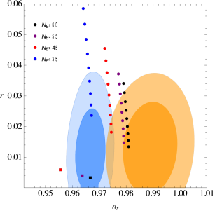
VII.5 Late-Time Alternative Proposed Models
VII.5.1 Bulk Viscous Models
The cosmological scenarios in which a fluid is endowed with a bulk viscosity is an effective description to alleviate the Hubble constant tension Wang:2017cel ; Yang:2019qza ; daSilva:2020mvk . A bulk viscous fluid is characterized by its energy density and pressure where this pressure term has two distinct components, namely, . The first component of the pressure term is the usual one , where is the EoS parameter of the fluid, and the second component characterizes the viscosity of the fluid defined by in which is the coefficient of the viscosity or the bulk viscous coefficient and is the four-velocity of the fluid Brevik:2005bj .
For any bulk viscous fluid, one can write down its evolution in the FLRW Universe as
| (10) |
where is the Hubble rate of the FLRW Universe. Thus, one can see that for different choices of the bulk viscous coefficient, , one can extract the constraints out of various cosmological scenarios. The cosmic fluid endowed by the bulk viscosity can either represent a DE fluid daSilva:2020mvk or a unified fluid which combines both DM and DE behaviours Yang:2019qza . The cosmological scenarios in which DE enjoys a viscous nature have been investigated in the literature aiming to address the Hubble tension Wang:2017klo ; Mostaghel:2016lcd ; Mostaghel:2018pia ; Velten:2012uv . The bulk viscosity coefficient characterized by Wang:2017klo leads to at 68% CL for the dataset Planck 2018 CMB distance priors + Pantheon + BAO + BBN + CC daSilva:2020mvk . For the bulk viscosity coefficient Mostaghel:2016lcd ; Mostaghel:2018pia , the Hubble constant takes the value at 68% CL for the combined dataset Planck 2018 CMB distance priors + Pantheon + BAO + BBN + CC daSilva:2020mvk . A different choice of the form Velten:2012uv can lead to at 68% CL daSilva:2020mvk for Planck 2018 CMB distance priors + Pantheon + BAO + BBN + CC. As the choice of the bulk viscous coefficient is not unique, one can therefore introduce a different parametrization to investigate the effectiveness of the models in the light of the Hubble constant tension.
Alternatively, a unified fluid endowed with bulk viscosity can increase the Hubble constant value. In this context, the bulk viscous coefficient ( is a real number) Velten:2012uv leads to at 68% CL Yang:2019qza (assuming a free with ) for the dataset Planck 2015 + Pantheon Yang:2019qza and at 68% CL (assuming both and are free parameters) for the dataset Planck 2015 + Pantheon Yang:2019qza .
On the other hand, an inhomogeneous cosmic fluid endowed with the bulk viscosity can also be considered as a possible scenario to alleviate the Hubble constant tension Elizalde:2020mfs . Using the Bayesian machine learning approach, the authors of Ref. Elizalde:2020mfs investigated two equation of state parameters representing an inhomogeneous cosmic fluid, namely, Model 1: ( are free parameters) and Model 2: ( are free parameters and is the deceleration parameter of the Universe). For Model 1, the Bayesian approach leads to at 68% CL (for the redshift interval ) and at 68% CL (for the redshift interval ). For Model 2, the Bayesian approach leads to at 68% CL (for the redshift interval ) and at 68% CL (for the redshift interval ).
VII.5.2 Chameleon Dark Energy
The chameleon field Khoury:2003aq ; Khoury:2003rn ; Wang:2012kj ; Upadhye:2012vh ; Khoury:2013yya ; Vagnozzi:2021quy ; Benisty:2021cmq can be considered to be a potential candidate for resolving the Hubble constant tension as recently explored in Ref. Cai:2021wgv . In addition to the screening effect from changing the effective mass of the chameleon field according to the ambient matter density, the chameleon field also admits a higher potential energy at its effective potential minimum (namely the vacuum energy) in the high-density regions than in the low-density regions. Hence, the over-densities would expand locally faster than the under-densities since there is more chameleon dark energy stored in the overdense regions. Therefore, the chameleon dark energy model Cai:2021wgv provides an environmentally dependent determination for the local Hubble constant. For a toy model with a top-hat density profile connecting an inner FLRW region to a outer FLRW region, a 10% matter over-density could raise the local value up to , while a 20% matter over-density could reach a local value as high as , which could be fitted precisely by the following approximation (here is the power of the Peebles-Ratra potential),
| (11) |
At large scales beyond Gpc, the matter homogeneity is well tested by the CMB data, therefore, the Hubble constant inferred from this scale simply recovers the CMB constraint on . At the intermediate scales of a few Mpc, the matter homogeneity is relatively poorly guaranteed due to the presence of some large-scale structures like voids Keenan:2013mfa and walls deLapparent:1985umo ; Gott:2003pf ; Lietzen:2016thc . Therefore, Ref. Cai:2021wgv also constructs a realistic model with a LTB metric to describe such intermediate inhomogeneities by explicitly counting the galaxy number excess from BOSS DR12 data Reid:2015gra ; Kitaura:2015uqa in each concentric spherical shells, however, the outcome is highly dependent on the adopted galaxy bias model Lavaux:2019fjr . At even smaller scales below Mpc, the matter homogeneity is obviously broken by computing the fractal dimension of galaxy number growth within a sphere, see e.g. Ref. Scrimgeour:2012wt . Using the distance indicators in the small-scale high-density regions (for example, SNIa in galaxies) would generally return back a higher value than the background. Similarly, calibrating the SNIa with Cepheids Riess:2016jrr ; Riess:2018byc ; Riess:2018uxu ; Riess:2019cxk ; Riess:2020fzl ; Riess:2021jrx generally renders a larger value than that with TRGB as the calibrator Freedman:2019jwv ; Yuan:2019npk ; Freedman:2020dne ; Soltis:2020gpl ; Freedman:2021ahq ; Anand:2021sum . This is because that most of TRGBs are specifically chosen to reside away from high matter density (for example, galaxy disk) to reduce large dust extinctions. Furthermore, the most recent improved measurements of strong lensing time delay from TDCOSMO+SLACS sample Birrer:2020tax favors a value closer to the background CMB value, which could also be explained within the picture of chameleon dark energy model by lensing objects that are specifically chosen in the under-density regions in order to diminish the effect from galaxy clusters. Note in end that since the chameleon dark energy drives the over-density region to expand faster so that the matter fluctuations smear at a larger scale until reaching a new virial equilibrium with lower matter density. This could shed the light on resolving the tension at the same time, which would require for a full time evolution formulation at perturbation level.
VII.5.3 Clustering Dark Energy
In clustering DE models, the sound speed of DE perturbations is much smaller than unity, allowing for non-negligible dark energy perturbations on scales well inside the horizon, see Ref. Batista:2021uhb for a review. Consequently, the growth of matter perturbations can be impacted by DE perturbations. Such models have been explored as a possible way to suppress Kunz:2015oqa .
In the limit , on small scales and during the matter-dominated era, DE perturbations follow matter perturbations according to the solution Abramo:2008ip ; Sapone:2009mb ; Creminelli:2008wc
| (12) |
Thus, the impact of clustering DE on depends on the . For non-phantom (phantom) models, DE perturbations are correlated (anti-correlated) to matter perturbations, enhancing (diminishing) . If at intermediate redshifts the is not very close to , DE perturbations can be of the same order of magnitude as matter perturbations. In this case, the impact of DE on matter growth is maximal.
Since DE perturbations can also contribute significantly to the gravitational potential, the associated perturbations should include its weighted contribution
| (13) |
The redshift evolution of for a given model M, , where is the growth function computed with can be largely affected by clustering DE. Normalizing to the CDM value at , Fig. 6 shows the evolution of for clustering and homogeneous DE models. Phantom clustering DE can potentially alleviate the tension, whereas the impact of non-clustering DE worsens it. But it is also possible that, for a given evolution of which provides a too low , clustering non-phantom DE can be used to increase it.
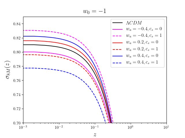
VII.5.4 Diffusion Models
A diffusive interaction between dark energy and dark matter was introduced in Refs. Haba:2016swv ; Koutsoumbas:2017fxp . In Ref. Calogero:2013zba , the authors formulate diffusion of energy density between dark energy into dark matter by using a non-conserved stress energy tensor with a source current ,
| (14) |
where is the coupling diffusion coefficient of the fluid. The current is a time-like covariant conserved vector field which describes the conservation of the number of particles in the system.
In a homogeneous expansion, the modified Friedman equations read:
| (15) |
The contribution of the current goes as since the current is covariantly conserved . In this way, there is a compensation between the dark energy and the dark matter. Ref. Perez:2020cwa claims that the diffusive interaction models can alleviate the Hubble constant tension with different types of matter fields.
Refs. Benisty:2017eqh ; Benisty:2017rbw ; Benisty:2017lmt ; Benisty:2018oyy formulate an action principle for these interactions starting from actions. The theory reads:
| (16) |
where is a scalar field. From a variation with respect to the vector field we obtain:
| (17) |
where is a current source for the stress energy momentum tensor . From the variation with respect to the new scalar , a covariant conservation of the current emerges:
| (18) |
Different expressions for which depends on different variables give the conditions between the Dynamical Spacetime vector field and the other variables. Cosmological implications are described in Ref. Benisty:2016ybt ; Benisty:2018qed ; Benisty:2018gzx ; Anagnostopoulos:2019myt ; Benisty:2020nql .
VII.5.5 Dynamical Dark Energy
Dropping the field interpretation of DE, it is possible to explore models in which DE sector deviates from the cosmological constant to a DE fluid with an extended EoS parameter , which can generally vary with redshift. These dynamical dark energy (DDE) models have been extensively studied in the literature Planck:2018vyg ; Zhao:2017cud ; Yang:2018qmz ; Yang:2018prh ; DiValentino:2019dzu ; Yang:2018qmz ; Vagnozzi:2019ezj ; Keeley:2019esp ; Joudaki:2016kym ; DiValentino:2017gzb ; Yang:2021flj ; Benisty:2021gde ; Roy:2022fif ; Sharma:2022ifr , based on considerations over the reconstruction of the effective from data Zhao:2017cud .161616However, low redshift data do not necessitate DDE Colgain:2021pmf . DDE models typically solve the tension within two standard deviations at the price of a phantom-like DE, i.e. , because of the geometrical degeneracy present with the DE EoS parameter . However, these models appear to worsen the growth tension of CDM Alestas:2021xes , while providing a worse fit to the BAO and SNIa data than CDM. In addition, they favor a value of SNIa absolute magnitude that is marginally consistent with Cepheid measurements Perivolaropoulos:2021jda ; Alestas:2021xes .
A particular Dynamical DE with a phantom crossing behaviour, as introduced in Ref. DiValentino:2020naf , seems to be able to solve the Hubble constant problem also when BAO and Pantheon data are considered, and at the same time alleviate the tension, see also Ref. Chudaykin:2022rnl .
VII.5.6 Emergent Dark Energy
A class of dark energy models in which dark energy has no effective presence in the past as it emerges at later times, usually dubbed as the emergent dark energy models Li:2019yem ; Pan:2019hac ; Rezaei:2020mrj ; Liu:2020vgn ; Li:2020ybr ; Yang:2020tax ; Benaoum:2020qsi ; Yang:2021eud , has received considerable attention in the cosmological community. In emergent dark energy models, the parametrization of the dark energy density is inserted into the Hubble equation as
| (19) |
where is the energy density of the DE fluid with respect to the critical energy density at present, namely . In Ref. Li:2019yem , the authors introduced a very simple emergent dark energy scenario, known as phenomenologically emergent dark energy (PEDE) scenario, where the dark energy sector evolves as
| (20) |
where . It is important to mention that within the PEDE scenario, even if the dark energy sector is dynamical, this scenario has exactly six free parameters as in the CDM model. For Planck 2018 alone, this model takes a very high value of the Hubble constant at 68% CL Yang:2020tax which is compatible with Ref. Riess:2020fzl within . Recently, in Ref. DiValentino:2021rjj , the PEDE model has been further confronted in the presence of the sterile neutrinos and perfectly agrees with the earlier observations Li:2019yem ; Pan:2019hac ; Yang:2020tax .
A generalization of the PEDE scenario known as generalized emergent dark energy (GEDE) introduces a dark energy evolution in terms of a free parameter as Li:2020ybr
| (21) |
While the symbol is a derived parameter representing the epoch where the matter energy density and the DE density are equal, that means equating, , one can derive . Although this scenario does not offer a very large value of the Hubble constant compared with its value estimated in the PEDE scenario, however, as explored in Ref. Yang:2021eud , within this GEDE scenario, the Hubble constant tension is reduced to with Riess:2020fzl (see also Hernandez-Almada:2020uyr ).
VII.5.7 Graduated Dark Energy - AdS to dS Transition in the Late Universe
The positive cosmological constant assumption of the CDM model was investigated via the graduated dark energy (gDE)—borrowed from the proposal of graduated inflation Barrow:1990vx —characterised by a minimal dynamical deviation from the null inertial mass density (where ) of the cosmological constant (or, the usual vacuum energy of QFT) Akarsu:2019hmw . This deviation is in the form of
| (22) |
for which, provided that the conditions (present-day energy density), (present-day inertial mass density), and with and being odd numbers are satisfied, the energy density dynamically takes negative values in the past Akarsu:2019hmw (see also Visinelli:2019qqu ). These three conditions lead to the gDE; the first two imply that gDE is in the phantom region in the late/present-day universe, and the last one causes the energy density to take negative values for redshifts larger than a certain redshift (see Ref. Akarsu:2019hmw for details). During the transition from negative to positive energy density as the Universe expands, there comes a time (or a redshift ) for which the energy density passes through zero and the EoS parameter exhibits a pole. The gDE in fact exhibits a wide variety of behaviors depending on , but it is of particular interest that for large negative values of , it establishes a phenomenological model characterized by a smooth function that approximately describes a cosmological constant which switches sign in the late Universe to become positive today.171717The case is called simple-gDE and investigated in Acquaviva:2021jov . The energy density of the gDE model, in terms of redshift, reads
| (23) |
where is a negative constant. Here ”” is the signum function that reads for , and , respectively. This expression indicates if there exists a sign change in the energy density of the gDE (accompanied by a pole in its EoS parameter Ozulker:2022slu ), it will happen at the redshift
| (24) |
around which, can exhibit a non-monotonic behavior. It was shown via the gDE that the joint observational data, including but not limited to the Planck CMB and Ly- BAO (BOSS DR11) data, suggest that the cosmological constant changed its sign at and triggered the late-time acceleration, the behaviour of which alleviates the tension by predicting and provides excellent fit to the Ly- BAO (BOSS DR11) data Blomqvist:2019rah at the effective redshift , which is at tension with the Planck 2015 best-fit CDM. Note that this tension is reduced to when the final eBOSS (SDSS DR16) measurement, which combines all the data from eBOSS and BOSS Blomqvist:2019rah ; eBOSS:2020yzd ; duMasdesBourboux:2020pck , is considered, see Sec. VIII.7.1.
Inspired by these observational findings, and the theoretically compelling fact that the gDE submits to the weak energy condition and the bounds on the speed of sound only in the limit which corresponds to a cosmological constant that rapidly changes sign at redshift , this limit was dubbed CDM and further investigated in Ref. Akarsu:2021fol . The CDM model can be constructed phenomenologically by simply replacing the usual cosmological constant () of the standard CDM model with a cosmological constant () that switches its sign from negative to positive, and thus attains its present-day value (), when the Universe reaches a certain energy scale (redshift ) during its expansion,
| (25) |
It was shown in Ref. Akarsu:2021fol that, when the consistency of the CDM model with the CMB data is guaranteed, (i) and (SNIa absolute magnitude) values are inversely correlated with and reach and for , in agreement with the measurements from SH0ES Riess:2016jrr ; Riess:2019cxk , and (ii) presents an excellent fit to the Ly- data provided that . The assessment of the model against Planck 2018 yields and against Planck 2018 + SDSS DR16 yields with Akarsu:2021fol . It was found that the lower and upper limits of are controlled by the Galaxy and Ly- BAO data, correspondingly, and the larger values imposed by the Galaxy BAO data prevent the model from achieving the largest estimations of from the direct local distance ladder measurements. It is intriguing that, as long as , the model remains in excellent agreement with the Ly- data even for , which barely satisfies the condition that we live in an ever-expanding Universe; a good agreement with the Ly- data is an intrinsic feature of the CDM model as long as .
Similar to the situation with the Ly- data, alleviating the discrepancy, prevailing within the CDM model and its minimal extensions, usually results in exacerbating the tension, see Sec. V and Ref. DiValentino:2020vvd . In addition to this, the constraints on based on the Ly- data are in agreement with the weak lensing surveys that probe similar late-time redshift scales as the Ly- measurements Palanque-Delabrouille:2019iyz . Accordingly, it is conceivable that the CDM model provides a remedy for the discrepancy while retaining the better fit to the local measurements of , like in the case of the Ly- discrepancy. Indeed, in the CMB-only analysis, it is found that for the CDM model, whereas for the CDM model. Although is smaller for the CDM model, its value greater than results in an increased value compared to its value. In contrast, the CDM model has an value lower than which results in a decreased value compared to its value. This results in the lower value of for CDM compared to CDM. The CDM and CDM models have similar values when the BAO data are also included in the analysis; this is due to the preference for larger values by the Galaxy BAO data, since CDM approaches CDM for larger values and the value of CDM becomes greater than 0.3. Thus, the CDM model partially reconciles the CMB data with the low redshift cosmological probes regarding , and can potentially resolve the discrepancy in the absence of the Galaxy BAO data; however, for a robust conclusion, the constraints on from low redshift probes should also be explored within the CDM model.
Ultimately, it turns out via the CDM model that sign switch in the cosmological constant, viz., transition from an Anti-de Sitter background (provided by ) to a de Sitter one (provided by ), at (i) relaxes the SH0ES tension while being fully consistent with the TRGB measurement, (ii) relaxes the tension, (iii) removes the discrepancy with the Ly- measurements, (iv) relaxes the tension, and (v) finds a better agreement with the BBN constraints on the physical baryon density Akarsu:2021fol . These results seem to encourage looking for a phase transition from AdS vacua to dS vacua in the late-Universe.
It is reasonable to look for a potential origin of this phenomenon, viz. a very rapid single transition or its limiting case a single instantaneous (discontinuous) transition in the value of the cosmological constant, in a theory of fundamental physics by considering it as a first-order phase transition. The phase transition approach has been used to address the tension; see e.g. Refs. Banihashemi:2018oxo ; Banihashemi:2018has ; Banihashemi:2020wtb , which consider that the DE density resembles the magnetization of the Ising model and present a realization of this behavior within the Ginzburg-Landau framework. Additionally, Ref. Farhang:2020sij considers a gravitational phase transition that is justified from the effective field theory point of view (see also Ref. Khosravi:2021csn ). The model studied in Ref. Banihashemi:2018oxo partially corresponds to a one-parameter phenomenological extension of CDM; it considers an arbitrary shift in the value of the cosmological constant, but does not allow negative values of the cosmological constant in contrast to CDM. It addresses the tension with a shift in the value of the cosmological constant, however, at very low redshifts, viz. , signaling that it could suffer from the tension Camarena:2021jlr ; Efstathiou:2021ocp (see also Refs. Alestas:2020zol ; Marra:2021fvf ; Alestas:2021luu ans Sec. VII.6.5). Given the promising advantages of having a negative cosmological constant for in light of cosmological tensions, and that negative cosmological constant is a theoretical sweet spot—AdS space/vacuum is welcome due to the AdS/CFT correspondence Maldacena:1997re and is preferred by string theory and string theory motivated supergravities Bousso:2000xa —it would be most natural to associate this phenomena with a possible phase transition from AdS to dS that is derived in string theory, string theory motivated supergravities, and theories that find motivation from them.
Besides, there is a rapidly growing literature on the cosmological models that suggest dark energy (as an actual source or an effective source from a modified theory of gravity) transitions in the late Universe from a negative (or vanishing) cosmological constant-like behavior to a positive cosmological constant-like behavior, accompanied by a pole in its EoS parameter. These models can relax the and tensions and/or the Ly- discrepancy, and the cosmological data either prefer or are fully consistent with the presence of a negative cosmological constant at high redshifts and the presence of a negative cosmological constant accompanying quintessence/phantom dark energy, see e.g. Refs. Sahni:2014ooa ; Poulin:2018zxs ; Wang:2018fng ; Mortsell:2018mfj ; Dutta:2018vmq ; Akarsu:2019ygx ; Bonilla:2020wbn ; Calderon:2020hoc ; LinaresCedeno:2021aqk ; Bag:2021cqm ; Escamilla:2021uoj ; Sen:2021wld .
VII.5.8 Holographic Dark Energy
DE motivated from the Holographic principle Li:2004rb ; Huang:2004mx ; Zhang:2014ija is widely known as Holographic DE (HDE). The model has been intensively investigated for its ability to explain the late-time cosmic acceleration (see the review Wang:2016och ). In the simplest (and original) HDE model, the DE density is given by
| (26) |
where is the radius of the future event horizon of the Universe and is the free parameter of the model. The holographic nature comes in the fact that appears in the dark energy density. In the simplest case therefore, such models have three parameters. There are many models based on variants of this theme which typically have more parameters (see Ref. Wang:2016och for a review). At late times when the DE is expected to dominate, the above HDE behaves like a cosmic fluid of EoS,
| (27) |
So, for , . It has been argued that HDE can also alleviate the Hubble constant tension, see e.g. Refs. Guo:2018ans ; Dai:2020rfo (see Ref. vanPutten:2017bqf for an earlier realisation), but as discussed in Ref. Colgain:2021beg this comes at the expense of violating the null energy condition, or having a turning point in . There are many extensions of the previous holographic model following either the Tsallis non-extensive entropy Tsallis:2012js ; Saridakis:2018unr , the quantum-gravitational modified Barrow entropy Barrow:2020tzx ; Saridakis:2020zol , or the Kaniadakis relativistic entropy Kaniadakis:2002zz ; Drepanou:2021jiv ; Hernandez-Almada:2021rjs . It has been discussed that the Hubble constant tension can be alleviated with Tsallis holographic dark energy daSilva:2020bdc or with Kaniadakis holographic dark energy Hernandez-Almada:2021aiw .
VII.5.9 Interacting Dark Energy
A cosmological scenario in which dark matter (DM) and DE share interactions other than gravitational leads to various interesting features Amendola:1999er ; Chimento:2003iea ; Cai:2004dk ; Barrow:2006hia ; Chen:2008ft ; Pettorino:2013oxa ; Pan:2012ki ; Kumar:2016zpg ; Nunes:2016dlj ; Pan:2016ngu ; Sharov:2017iue ; DiValentino:2017iww ; Kumar:2017dnp ; vandeBruck:2017idm ; Yang:2017zjs ; Yang:2017ccc ; Pan:2017ent ; Yang:2018pej ; Yang:2018euj ; Barros:2018efl ; Yang:2018xlt ; Yang:2018uae ; Yang:2018qec ; Yang:2019uzo ; Martinelli:2019dau ; Pan:2020zza ; DiValentino:2019ffd ; Teixeira:2019hil ; DiValentino:2019jae ; Teixeira:2019tfi ; Pan:2019jqh ; Paliathanasis:2019hbi ; Benevento:2020fev ; Gomez-Valent:2020mqn ; vandeBruck:2020fjo ; Lucca:2020zjb ; Yang:2020uga ; Yang:2019uog ; Pan:2020mst ; Yang:2018ubt ; Kumar:2021eev ; Lucca:2021eqy . In Ref. DiValentino:2019ffd ; DiValentino:2019jae ; Pan:2019gop ; Yang:2019uog ; Pan:2020bur ; Kumar:2021eev ; Nunes:2021zzi ; Gariazzo:2021qtg ; Guo:2021rrz , the authors have found that the IDE model can solve the tension with SH0ES within one standard deviation, leading to a preference for a non-zero DE-DM coupling at more than standard deviations, while fixing the DE EoS to a cosmological constant. However, this category can be further extended into two classes DiValentino:2019jae : (i) models with in which energy flows from DE to DM, (ii) models with in which energy flows from DM to DE. Related models can be realized in string theory Agrawal:2019dlm ; Anchordoqui:2019amx ; Anchordoqui:2020sqo .
A phenomenological description allows for the interaction between DE and another component, i.e. DM, which leads to an effective phantom-like EoS for DE. In more detail, we assume that the densities of DM and DE do not evolve independently but through a ”dark coupling” as Gavela:2009cy
| (28) | |||||
| (29) |
where and are the energy momentum tensors for DE and DM, respectively, while is the DM four-velocity in the DM frame. The quantity describes the interaction rate between the two dark sectors, and we specialise it here as , where is a (negative) dimensionless parameter that regulates the flow of DM into DE and . The background evolves as
| (30) | |||||
| (31) | |||||
| (32) |
where parametrizes the EoS for the DE component and is the total energy content of the Universe at a given time. The solution to Eq. (30) reads , where the effective EoS leads to a phantom-like EoS for . The DM-DE coupling term impacts on the evolution of perturbations Valiviita:2008iv ; Gavela:2009cy ; Gavela:2010tm and affects the observables in the CMB. In this view, the CDM model augmented with the DM-DE coupling, or CDM model, can be constrained from the observations of the CMB modes. The CDM model is characterized by the usual six cosmological parameters of CDM plus , namely .
The observations used for constraining the model consist of various independent measurements:
-
•
Measurements of the CMB temperature and polarization anisotropies, as well as their cross-correlations, from the Planck 2018 legacy data release (Planck TT,TE,EE+lowE) Planck:2018vyg ; Planck:2018lbu ;
-
•
Measurements of the CMB lensing power spectrum reconstructed from the CMB temperature four-point function Planck:2018lbu ;
-
•
Measurements of the Baryon Acoustic Oscillation (BAO) from the 6dFGS Beutler:2011hx , SDSS-MGS Ross:2014qpa , and BOSS DR12 eBOSS:2020yzd ; Alam:2016hwk surveys;
-
•
Measurements of the Type Ia Supernovae (SNIa) distance moduli from the Pantheon sample Pan-STARRS1:2017jku .
A Monte Carlo analysis of the CDM model that accounts for the Planck data alone leads to the value of the Hubble constant at 68% CL, which is a significant shift in the central value of the Hubble constant with respect to what obtained within the CDM model alone DiValentino:2019ffd . The value obtained is within from the value obtained from the observation of a sample of long-period Cepheids in the LMC by the Hubble Space Telescope Riess:2021jrx , and can thus be referred to as a possible solution to the tension. Incidentally, the method predicts a non-zero DM-DE interaction, with the parameter differing from zero by more than . When a joint analysis of the Planck+BAO or Planck+Pantheon datasets is considered, these results weaken and the tension with the HST results lies within the level. This mechanism is then not powerful enough to lead to a strong resolution to the tension.
Stepping away from phenomenological models, explicit examples of a DM-DE coupling can be built within models of supergravity. Of particular interest are models that admit a UV completion to a consistent theory of quantum gravity Addazi:2021xuf , based on satisfying a few key requirements that avoids such theories to lie in the swampland of inconsistent theories instead of in the string theory landscape of vacua Vafa:2005ui . Cosmological observations can come to hand in constraining swampland conjectures Akrami:2018ylq ; OColgain:2018czj ; Colgain:2019joh ; Kinney:2018nny ; Danielsson:2018qpa ; Anchordoqui:2021eox . Swampland conjectures generally make it difficult for fundamental theories based on compactification from extra dimensions to accommodate a period of accelerated cosmological expansion Montefalcone:2020vlu . Such a restriction can be avoided in models whose internal space is not conformally Ricci flat, as it is the case for the Salam-Sezgin model Anchordoqui:2020sqo . Within this supergravity model, dark matter could acquire a mass term which depends on the value of the quintessence field, thus realizing an effective DM-DE coupling which addresses the tension Anchordoqui:2019amx , in the so-called fading dark matter model Agrawal:2019dlm .
Apart from providing a valid solution to the tension, this class of cosmological models can also play an effective role in alleviating the tension.
For instance, one viable possibility to largely reduce the significance of the tension is to allow for DE-DM interactions in a scenario where the DE energy density can be transferred to the DM fluid via a coupling function proportional to the DE energy density itself (unlike the model able to address the tension, where the energy transfer is from the DM to the DE) DiValentino:2019jae ; Lucca:2021dxo (see also DiValentino:2019ffd ; Kumar:2019wfs ; Kumar:2021eev . Indeed, in this scenario, because of the additional energy flow from the DE to the DM over the cosmic history, a lower DM energy density with respect to the CDM model is allowed at recombination without a sizable effect on the shape of the CMB anisotropy power spectra. As a consequence, the redshift of matter-radiation equality decreases and since the peak of the matter power spectrum and its amplitude depend on this redshift, it follows that the whole matter power spectrum shits horizontally to larger scales and vertically to lower values (see Ref. Lucca:2021dxo and Fig. 1 therein for a more detailed discussion about this mechanism). As a result, after the inclusion of data from Planck 2018, BAO and Pantheon the model reduces the significance of the tension below the 2.5 level even for very discordant estimates. The addition of late-time data from weak-lensing surveys such as DES and KV450 further improves the concordance between early and late-time probes, without exacerbating the tension nor the overall fit to the data (feature also present when excluding late-time measurements).
Other possible DE-DM interaction scenarios involve for instance elastic interactions between the two fluids that only produce a momentum exchange Pourtsidou:2016ico ; Amendola:2020ldb ; Jimenez:2021ybe . In this scenarios, as is common in models where the DM has such interaction channels with other particles, the additional drag effect prevents the DM component from clustering, which results in a suppression of the matter power spectrum at relatively small scales. By comparing this model to data from Planck 2018, BAO and Pantheon one obtains that the mean value of the parameter does not change with respect to the CDM equivalent but the error bars are enlarged to the point where the tension largely disappears. The inclusion of late-time measurements such as from the Planck SZ cluster counts can then pick up the values of the distributions that bring the datasets in agreement, resulting in a clear detection of the interaction parameter, see Fig. 6 of Ref. Jimenez:2021ybe .
Finally, another possibility is an IDE model with a sign-changing interaction, as in Ref. Pan:2019jqh .
Note that in this Section the DM component enters only in relation to its interaction with DE. Models in which the interaction of DM with either the visible or other dark sectors affects the cosmological evolution are discussed below in Secs. VII.7.2 (cannibal DM), VII.7.15 and VII.7.3 (decaying DM models), VII.7.4 (dynamical DM), and VII.7.7 (interacting DM).
VII.5.10 Quintessence Models and their Various Extensions
The present accelerating expansion rate of the Universe can be brought forth by the presence of a light scalar field known as quintessence. The simplest of such models consists of minimally coupled scalar fields with a flat enough potential which, contrary to a cosmological constant, leads to a dynamical EoS parameter, Ratra:1987rm ; Caldwell:1997ii , see also Refs. Zlatev:1998tr ; Peebles:2002gy ; Copeland:2006wr ; Tsujikawa:2013fta for early reviews. The model building of quintessence fields as DE models with a field theory backend has recently featured extensively through string theory swampland conjectures Agrawal:2018own ; Palti:2019pca . Various extensions of the simple quintessence models such as coupled quintessence, in which DE sector couples to (dark) matter sector Amendola:1999er ; Agrawal:2019dlm ; Gomez-Valent:2020mqn or non-minimally coupled quintessence, in which the scalar field is coupled to gravity sector through non-minimal Capozziello:1999xt or non-minimal derivative Saridakis:2010mf couplings, and many other extensions Frieman:1995pm ; Choi:1999xn ; Nomura:2000yk ; Visinelli:2018utg ; Choi:2021aze ; Akrami:2017cir ; Akrami:2020zxw ; Akrami:2020zfz ; Eskilt:2022zky have been analysed. As quintessence models generally lead to and exacerbate the Hubble constant tension Vagnozzi:2019ezj ; Banerjee:2020xcn , these are generally not viable DE models. More generally, DE models with can be shown to be at odds with and tension Heisenberg:2022lob ; Heisenberg:2022gqk ; Lee:2022cyh .
VII.5.11 Running Vacuum Models
The persisting tensions between the CDM and some cosmological data (cf. Secs. IV and V) suggest that the rigid cosmological constant, , might be performing insufficiently at the observational level. It is tempting to check if we could alleviate some of these problems on assuming that the dark (or just vacuum) energy density might be (slowly) dynamical. A related option is to assume that the gravitational coupling can be mildly time-evolving. These possibilities may occur at a time or individually, but each has different implications on the local conservation laws. Rather than introducing some ad hoc phenomenological dependence of and as a function, say, of the cosmic time, we would like to have some more fundamental motivation for such a dependence. The Running Vacuum Model (RVM), see Refs. Sola:2013gha ; Sola:2015rra and references therein, may provide such a fundamental dynamics, emanating either from quantum field theory (QFT) or string theory. The RVM can implement any of the mentioned options and is characterized by a vacuum energy density, , which at the background level carries a mild dependence on the expansion rate and its time derivative. The relevant structure of the RVM for the current Universe reads as follows:
| (33) |
with , the local value of Newton’s constant, and the additive constant is fixed by the boundary condition (current value). The RVM at low energies has been tested repeatedly (and successfully) in the past, see e.g. Refs. Sola:2015wwa ; Sola:2016jky ; Sola:2017znb ; SolaPeracaula:2016qlq ; Sola:2017jbl ; Sola:2017jbl ; Sola:2018sjf ; Gomez-Valent:2017idt ; Gomez-Valent:2018nib ; Banerjee:2019kgu . The state-of-the-art phenomenological performance of the RVM has been presented in a recent study SolaPeracaula:2021gxi . The terms in Eq. (33) can only be important for the very early Universe as they can trigger inflation, but we shall not address the implications for the early Universe here (see Refs. Sola:2013gha ; Lima:2013dmf ; Sola:2015rra ; Sola:2015csa ; SolaPeracaula:2019kfm and references therein).
Theoretically, the structure of the RVM can be motivated from different perspectives, to wit: from the renormalization group in curved space-time Shapiro:2000dz ; Sola:2007sv ; Shapiro:2009dh , from scalar-tensor theories such as the Brans-Dicke theory of gravity with a non-vanishing SolaPeracaula:2018dsw ; deCruzPerez:2018cjx ; Sola:2019jek ; Sola:2020lba ; Singh:2021jrp , see Sec. VII.6.3, and also from QFT in curved space-time using adiabatic regularization and renormalization techniques Moreno-Pulido:2020anb ; Moreno-Pulido:2022phq . In addition, beyond the QFT approach, there recently exists an intriguing ”stringy” version of the RVM, which is based on the effective action of the bosonic part of the gravitational supermultiplet in string theory, see Ref. Mavromatos:2020kzj and references therein. At low energies, the stringy version makes the important prediction that DM should be axion-like but otherwise it behaves as the standard RVM. This means that the DE associated to the RVM is in both cases dynamical through a component (with ). In contrast, at high energies the stringy version nicely connects inflation with the physics of the primordial GWs, see Ref. Mavromatos:2020kzj for a comprehensive exposition and Ref. Mavromatos:2021urx for new developments in this direction.
The phenomenological performance of the RVM has last been discussed using the most up-to-date dataset available in Ref. SolaPeracaula:2021gxi , under the assumption . Neglecting the higher order terms, which are only relevant during inflation, Eq. (33) takes the form
| (34) |
where is the Ricci scalar. For this reason, we may call this form of the vacuum energy density (VED) the Ricci RVM, or just ”RRVM”.
This implementation has the double advantage of using one single parameter and provides a safe path to the early epochs of the cosmological evolution. In fact, when we approach the radiation dominated era we have and, hence, the impact of the running is highly suppressed in that epoch. We may consider two types of RRVM scenarios SolaPeracaula:2021gxi : type-I, in which the vacuum interacts with matter; and type-II, where matter is conserved at the expense of an exchange between the vacuum and a mildly evolving gravitational coupling . For type-I models we assume that the vacuum (”vac”) exchanges energy with CDM only: . Solving for the CDM and vacuum energy densities in terms of the scale factor yields
| (35) |
where and (i.e. includes the densities of CDM and baryons). As expected, for () we recover the CDM. For type-I models we admit also the possibility that the dynamics of vacuum is activated only very recently, namely at a threshold redshift , so that for . This possibility has been deemed plausible in the literature, see e.g. Ref. Martinelli:2019dau . We compare this option with the situation when there is no such threshold, see Fig. 7. As for type-II models, matter is conserved, but the vacuum can still evolve as long as the effective gravitational coupling also evolves with the expansion , starting from an initial value (which enters our fit). The approximate behavior of the VED for this model in the late-time Universe is:
| (36) |
The effective gravitational coupling evolves very mildly as in the current epoch (with of order ). The vacuum dynamics has also an important impact on the large scale structure (LSS) through the data. For a list of the main equations at the linear perturbation level, see Ref. SolaPeracaula:2021gxi .
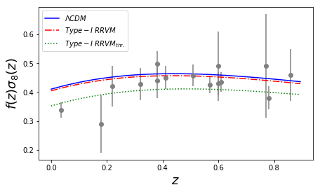
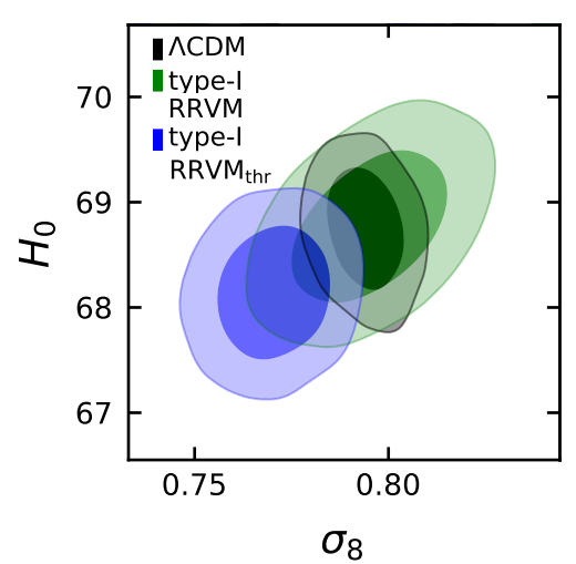
To compare the RRVM’s with the CDM, we have defined a joint likelihood function , where the total to be minimized in our case is given by . In particular, the part may contain or not the local value measured by the SH0ES team, but here we only present the results obtained by including it. Fig. 7 shows that the effect of the redshift threshold in type-I RRVM can be very important and suggests that a mild dynamics of the vacuum is welcome, especially if it gets activated at around the epoch when the vacuum dominance appears, namely at . Unfortunately, type-I models without such a threshold do not help to solve the tensions since the values of and remain very close to the CMB values SolaPeracaula:2021gxi . Nevertheless, this might not be a problem if the current expansion is slower than measured by SH0ES, as suggested e.g. in Refs. Freedman:2021ahq ; Mortsell:2021nzg ; Gomez-Valent:2018hwc ; Haridasu:2018gqm . In stark contrast, Fig. 10 shows that type-II models can alleviate the two tensions at a time. This variant of the RRVM provides values of markedly higher as compared to type-I models (specifically SolaPeracaula:2021gxi ) along with and values in the needed moderate range ( and ) SolaPeracaula:2021gxi . The values of in all RRVM’s are perfectly compatible with recent weak lensing and galaxy clustering measurements (cf. Ref. SolaPeracaula:2021gxi and Sec. V.1). The net outcome of this analysis is that of the two RRVM’s considered, only the type-II ones are capable of alleviating the two tensions ( and , whereas the type-I models with threshold redshift can (fully) solve the tension but have no bearing on the one. It is remarkable that the purely cosmographic analyses (which are more model-independent) also favor the RVM option as compared to other models of the dark energy Rezaei:2021qwd .
VII.5.12 Time-Varying Gravitational Constant
Seminal work of Weinberg suggests that an effective quantum theory of gravity would be asymptotically safe, with the renormalization group equations possessing a fixed point Weinberg1978 ; Weinberg:2009wa . A consequence of this framework is an extension of the CDM model in which Newton’s gravitational constant could depend on time Xue:2014kna ; Begue:2017lcw . In more detail, in this model the gravitational coupling is a function that varies with redshift as , such that is the value today, the suffix ”0” refers to the present time values, and parametrizes the change in the gravitational constant. As a consequence, the cosmological constant would also be redshift-dependent and follows a scaling law, . The matter ”” and radiation ”” contents would satisfy the scaling relations
| (37) | |||||
| (38) | |||||
| (39) |
The requirement for a flat Universe leads to the relation
| (40) |
The assessment of the model against cosmological data is performed in Ref. Gao:2021xnk . In particular, two realizations of this model are considered, namely the CDM model in which Eq. (40) is enforced, and the eCDM model in which and are kept as independent parameters. Both models cannot ease the tension in the Hubble constant when using an analysis that uses the combination of Planck 18 TT,TE,EE+lowE+lensing data Planck:2018vyg plus BAO plus data from SN1e Pantheon compilation Pan-STARRS1:2017jku . The tension is reduced when the measurement of by the SH0ES team is used as a Gaussian prior. Recently, it has been speculated that the Hubble tension could be resolved within the stochastic quantization formalism of gravity Lulli:2021bme , although more work is required along this direction.
Other approaches considering varying gravitational constant are analysed in Sakr:2021nja , that considering as a free parameter, and in Maeda:2022ozc in the context of a cuscuta-galileon gravity theory. Finally, Ref Benevento:2022cql implements a sharp transition in the value of the effective gravitational constant prior recombination, effectively lowering the sound horizon at CMB last scattering and addressing both the and the tensions. Assessing the model against Planck 2018 TT,TE,EE + LowE and BAO data, the value inferred for the Hubble constant is Benevento:2022cql .
VII.5.13 Vacuum Metamorphosis
The Vacuum Metamorphosis (VM) model is motivated by the fact that quantum gravitational effects Parker:2003as ; Parker:2000pr ; Caldwell:2005xb can significantly increase the Hubble constant value leading to a solution for the Hubble tension DiValentino:2017rcr ; DiValentino:2020kha ; DiValentino:2021zxy ; DiValentino:2021rjj . This model is a first principles theory based on a late-time gravitational phase transition that takes place when the Ricci scalar curvature is of the order of the squared mass of the scalar field, , and is related to the matter density today, . For this reason, the VM model has the same number of degrees of freedom as the CDM scenario.
The expansion rate before and after the phase transition result in DiValentino:2020kha :
| (41) |
with , , and the redshift of the phase transition
| (42) |
In other words, after the phase transition the Universe effectively has a radiation component that rapidly redshifts away leaving the Universe in a de Sitter phase, and therefore it is not nested with the CDM scenario.
In the original Vacuum Metamorphosis scenario described above, there is not a cosmological constant at high redshifts and therefore
| (43) |
It is also possible to extend this VM model assuming a possible cosmological constant at high redshifts, as the vacuum expectation value of the massive scalar field. In this case, we have to impose the additional conditions , i.e. the transition happening in the past, and . With both the VM model and its extension, the Hubble constant is completely in agreement with the SH0ES value, without assuming a Gaussian prior on it. Unfortunately this model fails to fit in a good way the low redshift data, such as BAO and Pantheon: remains in the SH0ES range but with a much worse than CDM.
VII.6 Modified Gravity Models
Modified gravity (MG) models Clifton:2011jh ; Planck:2015bue in which some feature of gravity (such as the gravitational coupling) changes with redshift, can lead to an estimate from CMB larger than that obtained from late-time probes Umilta:2015cta ; Ballardini:2016cvy ; Raveri:2019mxg ; Yan:2019gbw ; Frusciante:2019puu ; Frusciante:2020gkx ; Sola:2019jek ; Sola:2020lba ; Ballesteros:2020sik ; Braglia:2020iik ; Ballardini:2020iws ; Rossi:2019lgt ; Joudaki:2020shz ; Braglia:2020auw ; Akarsu:2019pvi ; Benetti:2018zhv . To solve (or at least relax) the tension in the context of MG models, instead of modifying the matter content, the gravitational sector is modified in a manner that current cosmic dynamics is derived. In particular, it is easy to argue that Newton’s constant needs to decrease as the Universe evolves in order to stand a chance of resolving cosmological tensions Heisenberg:2022lob ; Heisenberg:2022gqk ; Lee:2022cyh . There has been several proposals in GR that follows this line of thought Clifton:2011jh ; Ishak:2018his . One interesting approach in this direction has been the theories Sotiriou:2008rp ; Faraoni:2008mf ; DeFelice:2010aj , in which an arbitrary function of the Ricci scalar replaces the standard Einstein-Hilbert Lagrangian density. In the metric version, the Ricci scalar and the metric tensor evolve in time in an independent fashion. Thus, there is a scalar degree of freedom (absent in GR), which helps to explain the late cosmic acceleration and structure formation without the need of the dark matter sector.181818In the Palatini version, the same result is achieved due to the new terms that arise from the affine connection when written in of the Christoffel symbols and of the quantities that describe the matter Sotiriou:2008rp . Along with various cosmological models in Einstein gravity, the modified gravity models can also reconcile the tension Planck:2015bue ; DiValentino:2015bja ; Joudaki:2016kym ; Joudaki:2017zdt ; Sola:2019jek ; Sola:2020lba ; Wen:2021bsc .
VII.6.1 Effective Field Theory Approach to Dark Energy and Modified Gravity
Above we have discussed several alternatives to a purely cosmological constant in late-time cosmology, e.g., modified gravity. Much of these alternatives are often very model specific and must confront precise observations. Given the current wealth of data another theoretical approach – motivated by techniques utilized in particle and condensed matter physics – is to utilize methods of effective field theory as applied to cosmology Park:2010cw ; Gubitosi:2012hu ; Bloomfield:2012ff . This can also lead to an effective method to confront a large, and much general set of models with observations Wen:2021bsc ; Frusciante:2013zop ; Raveri:2014cka .
This approach is to establish how gravity may, or may not, be modified to explain the current acceleration of the expansion of the Universe and at what scales this is relevant (e.g. it is well known that gravity cannot be modified at solar system scales). In the effective field theory approach, one can establish groups of models to collect model dependent approaches and establish these into groups of models independent (universality classes) based on their symmetries (or lack thereof). This allows for a method to connect a large model specific set of predictions to be confronted with observations. For example, Horndeski models (mentioned above) are of broad interest in the community, but in this formalism, they form a universality class that can be viable or ruled out by current and near-term observations.
VII.6.2 Gravity
Recently, teleparallel gravity (TG) and its extensions have started to take advantage of their mathematical description to solve the tension and describe the cosmic late-time dynamics with current data. In these kind of theories, gravity is still described in geometrical terms, but using torsion instead of curvature, namely using the Weitzenböck connection Weitzenbock1923 instead of the Levi-Civita one. Hence, the actions of GR and TG differ only by a boundary term, and thus they lead to the same equations, that is why the corresponding theory is called Teleparallel equivalent of General Relativity (TEGR). There are several ways to modify the TEGR proposal: (1) through the so-called torsion scalar Nunes:2018xbm . In this form, we can generalise the Lagrangian to arbitrary functions of the torsion scalar to produce gravity Ferraro:2006jd ; Linder:2010py ; Chen:2010va ; Benisty:2021sul ; Bahamonde:2022ohm , analogous to theories (for reviews see Cai:2015emx ; Bahamonde:2021gfp ). (2) Furthermore, the importance of the boundary term, gravity models has also been well-studied Escamilla-Rivera:2019ulu ; Bahamonde:2015zma ; Farrugia:2018gyz as a possible extension to TEGR to infer Escamilla-Rivera:2019ulu . Performing consistency tests with current astrophysical data allows to identify a gravity theory and deal at the same time with systematic effects in the observational data. In some cases, data samples are sensitive to the geometry and dynamics of the Universe and other samples are sensitive to the growth of LSS. In such cases, these two sets of observations must be consistent with one another in order to solve the cosmological tension inside a specific model. At late-times, any deviations between models can be measured through an effective EoS that mimics a dark energy component near to the CDM EoS value (). In Ref. Escamilla-Rivera:2020ges it was provided an insightful test via examples in and gravity theories that can solve the tension using current late-time surveys (see also Refs. Lambiase:2018ows ; Benetti:2019smr ; Cai:2019bdh ; DAgostino:2020dhv ; Wang:2020zfv ; Parashari:2021qjg ). Theories that deviate from GR can be delineated into categories according to what principle or requirement they violate. Theoretical efforts to find a dynamic model describing the data have been placed side by side to kinematic models, as the cosmography, where the current expansion is a function of the cosmic time Sahni:2014ooa ; Capozziello:2019cav ; Benetti:2019gmo ; ElHanafy:2020pek .
In its most simple formulation, it is possible to consider extensions of teleparallel gravity intended as corrections to TEGR where only the torsion scalar is considered. The action takes the form of
| (44) |
where is the reduced Planck mass, is a generic function of the torsion scalar , is the action of matter fields, and the tetrad is the metric determinant.
For a flat FLRW background, it is possible to derive the relation between the torsion and the Hubble parameter, . The sign of such a torsion element depends on the signature of the metric, which is identified by the vierbien fields . Assuming that matter sector is described by a perfect fluid with energy density and pressure , the field equations give
| (45) | |||
| (46) |
Moreover, the set of equations is closed with the equation of continuity for the matter sector . Eqs. (45)-(46) can be rewritten in terms of the effective energy density and pressure arising from ,
| (47) | |||
| (48) |
and define the effective torsion equation-of-state
| (49) |
These effective models are hence responsible for the accelerated phases of the early or/and late Universe Cai:2015emx .
In order to study the background evolution, we can rewrite the first FLRW equation, making explicit the form of the torsional energy density Nesseris:2013jea ; Nunes:2018xbm ; Nunes:2016qyp
| (50) |
where we considered the relation and is the present value of .
At this point, specific forms of functions must be chosen and several in the literature have passed basic observational tests Nesseris:2013jea ; Nunes:2016qyp ; Capozziello:2017bxm ; Nunes:2018xbm ; Briffa:2021nxg . Between them, the simplest form of power-law proved to be the one that predicts an compatible with Cepheids observations Riess:2019cxk . This model is described by Nesseris:2013jea
| (51) |
Inserting this form into (45) and for and , the scenario reduces to CDM cosmology, namely .
Analysing this model considering both the background and the linear perturbation evolution, in the light of both large and small scale data, a value of has been constrained using CMB+lensing+BAO+R19+Pth+DES data Benetti:2020hxp (see Ref. Briffa:2021nxg for for analysis with several other combinations of large-scale data). Also, a deviation from the GR was detected at more than . Noteworthy, this allows to significantly relax the Hubble constant tension, but worsens tension MacCrann:2014wfa ; Battye:2014qga ; Benetti:2017juy since the correlation of the two parameters does not seem to be removed from this treatment of models.
Let us now try to suitably extract an form that could alleviate bothe tensions simultaneously. In order to avoid the tension one needs a positive correction to the first Friedmann equation at late times that could yield an increase in compared to the CDM scenario. As for the tension, since at sub-Hubble scales and through the matter epoch, the equation that governs the evolution of matter perturbations in the linear regime is
| (52) |
where is the effective gravitational coupling. Thus, alleviation of tension may be obtained if becomes smaller than during the growth of matter perturbations. In the case of gravity the effective gravitational coupling is given by Nesseris:2013jea
| (53) |
According to the Effective Field Theory approach to gravity Li:2018ixg ; Yan:2019gbw ; Ren:2022aeo one can choose in order to obtain a Hubble function evolution of the form
| (54) |
where is the Hubble rate in CDM after recombination, is the present matter density parameter, and primes denote derivatives with respect to . The function can be selected to be in order to have , therefore the tension is solved. One should choose , and thus, since decreases for smaller , the deviation from CDM will be significant only at low redshift]. Additionally, since becomes smaller than during the growth of matter perturbations, the tension is also solved.
We follow Ref. Yan:2019gbw and we consider the ansatz , where describes the deviation from GR (mind the difference in the conventions). Under these assumptions, the first Friedmann equation becomes
| (55) |
In order to solve the tension, we need , with following results with local measurements Riess:2019cxk , while in the early era of we require the Universe expansion to evolve as in CDM, namely . This implies (the value corresponds to standard GR, while for we obtain CDM too). Therefore, the perturbation equation at linear order becomes
| (56) |
Since around the last scattering moment the Universe should be matter-dominated, we impose , while at late times we look for that leads to an in agreement with redshift survey observations.
By solving Eqs. (55) and (56) with initial and boundary conditions at and , we can find the form that can alleviate both and tensions. In particular, we find that we can fit the numerical solutions very efficiently through , dubbed Model-1, and , dubbed Model-2. We examine , and as expected we find that at high redshifts in both models, becomes , recovering the CDM paradigm. We have checked that both models can easily pass the BBN constraints, which demand Copi:2003xd , as well as the ones from the Solar System, which demand and Nesseris:2006hp .
In Fig. 8 we present the evolution of , while in Fig. 9 the evolution of , for two models, and we compare them with CDM. We stress that the tension can be alleviated as remains statistically consistent for all CMB and CC measurements at all redshifts. We remind the reader that the two models differing merely by a term , which does not affect the background as explained before, are degenerate at the background level. However, at the perturbation level, the two models behave differently as their gravitational coupling differs.
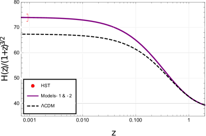
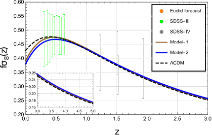
We further stress that both models can alleviate the tension, and fit efficiently to BAO and LSS measurements. Note that at high redshifts (), Model-2 approaches CDM slower than Model-1, but in a way that is statistically indistinguishable for present-day data. Nevertheless, future high-redshift surveys such as eBOSS for quasars and Euclid EUCLID:2011zbd for galaxies have the potential to discriminate among the predictions of gravity and the CDM scenario. Moreover, the clusters and CMB measurements on are in good agreement in our models, as the CMB preferred values in CDM get further lowered than local ones from rescaling by the ratio of the growth factors in gravity and CDM. In more detail,
| (57) |
where is the growth factor, and denote the models for modified gravity and CDM, respectively, and is the effective redshift of the measurements, with for clusters experiments and for CMB temperature fluctuations observations. At high redshifts , the growth factor is the same in both the model and in CDM, while at low redshifts , the growth factor is approximately 1.03 times bigger in the latter one. For this reason, cluster -measurements increase by about the same factor, reducing the gap with CMB preferred value in this modified gravity scenario.
In summary, we conclude that the class of gravity described by
| (58) |
where only two out of the three parameters , , and are independent (the third one is eliminated using ), can alleviate both and tensions with suitable parameter choices. Moreover, these type of gravity models could also be examined through galaxy-galaxy lensing effects Chen:2019ftv , strong lensing effects around black holes Yan:2019hxx , and GW experiments Cai:2018rzd .
VII.6.3 Horndeski Theory
Shift-Symmetric Horndeski Theories.
After the detection of the gravitational-wave event GW170817 LIGOScientific:2017vwq and its electromagnetic counterpart, the speed of GWs is constrained to be very close to that of light . Without the shift symmetry condition, namely that the theory is invariant under scalar shifts, with constant , Horndeski would reduce to three functions, , and (for example, see Ref. Kase:2018aps ). Further imposing the shift symmetry condition, and are reduced to functions of only, while becomes a constant. The Lagrangian of the Horndeski theories Horndeski:1974wa ; Kobayashi:2011nu ; DeFelice:2011bh ; Kobayashi:2019hrl realizing this condition is strongly constrained Ezquiaga:2017ekz , in particular the cubic-order shift-symmetric Horndeski theories falls back in this class of theories. The cubic-order shift-symmetric Horndeski action is given by Kobayashi:2019hrl
| (59) |
where is the determinant of the metric tensor , is the reduced Planck mass, is the Ricci scalar, and , are functions of , with being the scalar field. Finally, corresponds to the action of standard th fluid fields . The continuity equations of fluids reads on the FLRW background,
| (60) |
where is the fluid density, is the constant barotropic coefficient relating the fluid density and the pressure, is the Hubble expansion rate, and a dot stands for the derivative with respect to . We recall that the modified Friedmann and scalar-field equations at at the background level are given by
| (61) | |||
| (62) | |||
| (63) |
The density and pressure of the scalar field are obtained as
| (64) | |||||
| (65) |
with . From this, we can define a scalar field EoS as
| (66) |
From Eq. (61), there is the constraint , where . Finally, by solving Eqs. (62)-(63) for and one can know the dynamics of the Universe. For linear perturbations we consider the perturbed FLRW line element: , where and are the gravitational potentials and for the perturbations in the matter sector follow the standard perturbation theory Ma:1995ey . In the case of modified gravity, in order to derive an explicit relation between the gravitational potentials and the matter perturbation , one has to use the quasi-static approximation (QSA) Boisseau:2000pr ; Tsujikawa:2007gd ; DeFelice:2011hq ; Sawicki:2015zya which, within the Horndeski class of models, it is a valid assumption for the wavenumber in the range Peirone:2017ywi ; Frusciante:2018jzw . In this approximations one has:
| (67) | |||||
| (68) |
where is Newton’s gravitational constant. The dimensionless quantities and characterize the effective gravitational couplings felt by matter and light, respectively. For the cubic-order shift-symmetric Horndeski theories one has and DeFelice:2011hq ; Kase:2018aps
| (69) |
where the kinetic term and the speed of propagation of the scalar field are given by
| (70) | |||||
| (71) |
Both the above quantities need to be positive defined to avoid Ghost and Gradient instabilities. Finally the matter perturbation equations can be written as
| (72) |
In the following we specialize to two models which are of interest for alleviating the tension.
-
•
Galileon Ghost Condensate (GGC): We consider the Galileon Ghost Condensate (GGC) model which is specified by the functions Deffayet:2010qz ; Kase:2018iwp
(73) where , , are constants. This model departs from the Cubic Galileon model Deffayet:2009wt by the inclusion of the term , which affects the cosmic expansion history and growth of structures at both linear Kase:2018iwp ; Peirone:2019aua and non-linear scales Frusciante:2020zfs compared to . The presence of nonvanishing allows to prevent the solutions from approaching the tracker at background level. In this case it is possible to realize the phantom behaviour for the scalar field () without having ghosts Kase:2018iwp ; Peirone:2019aua . At linear perturbation and in Eq. (69) are larger than 1, so both and are enhanced compared to those in GR, showing a stronger gravitational interaction. In particular, it has been found that the model suppresses the large-scale CMB temperature anisotropy in comparison to the CDM model. These features lead to the statistical preference of GGC over CDM when data from CMB, BAO, SNIa, and RSDs are used Peirone:2019aua . Furthermore the CMB temperature and polarization data from Planck 2015 release lead to an estimation for today’s Hubble parameter with is higher than the CDM and consistent with its direct measurements at 2, at 95% CL with best fit Peirone:2019aua .
-
•
Generalized Cubic Covariant Galileon (GCCG): Let us consider the Generalized Cubic Covariant Galileon (GCCG) model DeFelice:2011bh , defined by the functions
(74) where , , , are dimensionless constants, and , are constants having dimension of mass. For simplicity another parameters are used defined by and . The GCCG model is an extension of the Covariant Galileon (, ), and the same as the latter, it also allows for the existence of a tracker solution following the relation with . For this model it is possible to verify that for any viable value of and and hence the gravitational interaction is always stronger than in GR.
Observational constraints on , in the case of Planck 2015 alone are: at 95% CL, finding a consistency with its determination from Cepheids at 1 Frusciante:2019puu . Such result on is also compatible with the estimation obtained with the tip of the red giant branch in LMC, Yuan:2019npk . The main feature behind the eased tension in the GCCG model is due to a modified low redshift expansion history which is enhanced with respect to CDM. In this model is also interesting to note that if the tension between CMB data and low redshift measurements of disappears for the GCCG model, another tension between the latter and BAO data appears Frusciante:2019puu (see also Renk:2017rzu ).
Horndeski Theories with Non-Minimal Derivative Coupling.
Let us now examine one interesting subclass of Horndeski gravity, or equivalently generalized Galileon theory, that contains the term of the corresponding action, which is called ”non-minimal derivative coupling term”. Thus, instead of Eq. (59), we consider the action Saridakis:2010mf ; Petronikolou:2021shp
| (75) | |||||
where is the Einstein tensor. The Friedmann equations in FLRW geometry become DeFelice:2011bh
| (76) | |||||
| (77) |
while the scalar-field equation is , with and . Finally, the conditions in Eqs. (70)-(71) for absence of Laplacian and ghost instabilities become:
| (78) | |||||
| (79) |
with
| (80) | |||||
| (81) | |||||
| (82) | |||||
| (83) |
In order to alleviate the tension using the above construction we need to obtain a weakening of gravity at low redshifts by the terms depending on the scalar field’s kinetic energy. We impose a simple scalar field potential and standard kinetic term, thus , and we will consider the term to be shift-symmetric, i.e. . We consider two models.
-
•
Model I: In this case, the Friedmann Eqs. (76)-(77) become
(84) (85) We choose the model parameter and the initial conditions for the scalar field in order to obtain and , in agreement with the results from Planck 2018 Planck:2018vyg , and we leave as the parameter that determines the late-time deviation from CDM cosmology necessary to alleviate the tension. Choosing in Planck units leads to and thus the tension is indeed alleviated, while remains almost equal to 1 and remains positive, and therefore the scenario is free from pathologies Petronikolou:2021shp .
-
•
Model II: In this case the Friedmann Eqs. (76)-(77) become
(86) (87) Choosing in Planck units leads to , while remains almost equal to 1 and remains positive Petronikolou:2021shp . Hence the Hubble tension is alleviated.
In summary, we showed that the above particular sub-class of Horndeski/generalized Galileon gravity can alleviate the tension due to the effect of the kinetic-energy-dependent term. In particular, at early times the field’s kinetic term is negligible and hence the terms do not introduce any deviation from CDM scenario, nevertheless as time passes they increase in a controlled and suitable way in order to make the
Hubble function, and thus too, to increase.
However, see Refs. Banerjee:2020xcn ; Lee:2022cyh , where it is argued that DE models in a general class of scalar-tensor theories, including quintessence and a good class of Horndeski theories, perform worse than CDM model as far as the increasing is concerned. Moreover, a similar result is discussed in Refs. Heisenberg:2022gqk ; Heisenberg:2022lob where it is argued that the family of scalar-tensor DE models generically exacerbate and anomalies. A further problem of the Horndeski models with non-minimal derivative coupling, i. e. , is that to evade constraints from gravitational waves LIGOScientific:2017vwq , some fine tuning is required.
Minimal Scalar-Tensor Theories of Gravity.
The action for the simplest scalar-tensor theories of gravity within the most general Horndeski model Horndeski:1974wa with a scalar field in units of the reduced Planck mass and non-minimally coupled (NMC) to the Ricci curvature is Capozziello:1994du ; Boisseau:2000pr ; Esposito-Farese:2000pbo ; Nesseris:2006jc ; Cai:2009zp
| (88) |
where is a generic function of . Examples include induced gravity (IG), i.e. where is the coupling to the Ricci scalar, and conformally coupled scalar field (CCSF), i.e. where is a dimensionless parameter. A scalar-tensor theory allows to easily attain values for that are larger than in CDM. This effect is mainly due to a degeneracy between the coupling to the Ricci curvature and and is connected to the rolling of the scalar field, which regulates the gravitational strength, at the onset of the matter dominated era driven by pressureless matter. Therefore, larger values for can appear already in archetypal models of scalar-tensor theories of gravity, namely Jordan-Brans-Dicke (JBD) models BransDicke1961 ; Dicke1962 , see Sec. VII.6.3 for additional detail. This effect is a) largely independent on the part of the scalar field potential which acts as an effective cosmological constant, b) robust with respect to uncertainties in the neutrino sector, and c) possibly enhanced by allowing a difference between the gravitational constant relevant for cosmology and Newton’s constant as measured in a Cavendish-like experiment.
The possibility to connect a larger value of with an early-time modification of GR in the context of scalar-tensor gravity has been highlighted since the first Planck 2013 data release, where one of the simplest scalar-tensor gravity model, such as induced gravity (equivalent to JBD) with a quartic potential has been studied Umilta:2015cta , showing the degeneracy between the coupling to the Ricci scalar and . Subsequent studies updated and generalized this result for different simple potentials and couplings Ballardini:2016cvy ; Rossi:2019lgt ; Ballesteros:2020sik ; Ballardini:2020iws ; Ballardini:2021eox .
To sum up, for an effectively massless () scalar field at rest in the radiation era and with adiabatic initial condition for the scalar field perturbations Paoletti:2018xet , the current constraints on the Hubble parameter from Planck 2018 data (temperature, E-mode polarization, and CMB lensing) at 68% CL are for IG and for CCSF, respectively Ballardini:2020iws . When BAO data from BOSS DR12 are added, the constraint at 68% CL becomes for IG and for CCSF. Once a Gaussian likelihood based on the determination of the Hubble constant from the SH0ES team is also included, i.e. Riess:2019cxk , we obtain at 68% CL for IG and at 68% CL for CCSF. These constraints have been obtained by fixing the value of the scalar field today to
| (89) |
where and , in order to guarantee that the effective gravitational constant today corresponds to the value of the bare gravitational constant (Boisseau:2000pr, ).191919See Refs. Avilez:2013dxa ; Akarsu:2019pvi ; Joudaki:2020shz ; Ballardini:2021evv for studies of these models without imposing this condition.
NMC models with and a generic negative value of the coupling have been explored in Rossi:2019lgt ; Ballesteros:2020sik ; Braglia:2020iik ; Ballardini:2020iws ; Abadi:2020hbr , where the scalar field decreases from an initial value to a final value close to zero, so that the Newton’s constant changes after BBN from a value to the present value . Such models were shown to lead to , with , and a marginal improvement of compared to CDM, at the cost of 2 extra parameters (with Planck 2018, BAO, SH0ES 2019 and Pantheon, plus Solar system constraints) Ballesteros:2020sik , or with , and a more significant improvement with 2 extra parameters (with Planck 2018, BAO, SH0ES 2019 and Pantheon), when ignoring Solar system constraints Ballesteros:2020sik .
Finally, NMC models have been studied in presence of an effective mass in Ref. Braglia:2020auw . In this Early Modified Gravity (EMG), the scalar field, which is frozen during radiation era, grows around the time of recombination driven by the coupling to pressureless matter and is subsequently driven into damped oscillations around its minimum at by the small effective mass induced by a quartic potential. In addition to providing a better fit to cosmological datasets compared to the CDM model and EDE models, in the EMG model the positive branch for also satisfies automatically the tight constraints on the gravitational constant from laboratory experiments and Solar System measurements on post-Newtonian parameters thanks to the fast rolling of the scalar field towards the bottom of the potential. For this model with and , we obtain and combining Planck 2018, BAO and the full shape information from BOSS DR12, SH0ES 2019, and Pantheon SNe.
Minimally and non-minimally coupled scalar field models can also potentially decrease the tension. Minimally coupled models can be classified via their barotropic EoS parameter, . The models with are referred to as quintessence models, while the models with are referred to as phantom models. When a coupling between the scalar field and the Ricci scalar is allowed one has the so-called NMC quintessence models or scalar-tensor theories. In the literature, scalar-tensor theories have been studied as possible solutions to the tension, since under certain circumstances they can produce a reduced growth rate compared to the standard one in the context of GR that seems to be required by different dynamical data Macaulay:2013swa ; Hildebrandt:2016iqg ; Nesseris:2017vor ; Kohlinger:2017sxk ; Joudaki:2017zdt ; DES:2017myr ; Kazantzidis:2018rnb ; Perivolaropoulos:2019vkb ; Kazantzidis:2019dvk ; Skara:2019usd ; Asgari:2019fkq ; Joudaki:2020shz ; Heymans:2020gsg . This behaviour can be attributed either to the reduction of the parameter or to the existence of an evolving Newton’s constant giving at low .
Ref. Davari:2019tni showed that the constraints on the – plane are affected when considering these classes of models. In particular, while minimally coupled models simply feature a different background evolution, NMC models possess a qualitatively different growth of perturbations as the perturbation equation is modified by replacing Newton constant that appears in the Einstein action of GR with the effective gravitational constant that would be measured in Cavendish-like in the context of ST theories expressed as Boisseau:2000pr ; Esposito-Farese:2000pbo ; Nesseris:2006jc ,
| (90) |
which is a generalization of Eq. (89). In Ref. Davari:2019tni it is found that minimally and NMC models give similar constraints on the – parameter plane and lower values of as compared to the standard CDM model. However, this is done considering specific forms of the scalar field potential and non-minimal coupling function, a more general ansatz could relieve the tension.
In the context of an evolving Newton’s constant at low , it has been shown that various mechanisms can produce weaker gravity (), such as a scalar-tensor theory in a CDM background with Gannouji:2018ncm ; Perivolaropoulos:2019vkb ; Kazantzidis:2019dvk as well as more general modified gravity theories involving scalar fields such as Horndeski theories Linder:2018jil ; Kennedy:2018gtx ; Gannouji:2020ylf and beyond Horndeski theories DAmico:2016ntq . In Refs. Nesseris:2017vor ; Kazantzidis:2018rnb ; Perivolaropoulos:2019vkb ; Kazantzidis:2019dvk the following purely phenomenological parametrization that takes into account the solar system Pitjeva:2021hnc ; Will:2005va ; Uzan:2002vq and Big Bang Nucleosynthesis constraints Alvey:2019ctk ; Uzan:2002vq , has been proposed as a possible solution to the growth tension
| (91) |
where is an extra parameter and is an integer constrained at due to solar system tests. It is straightforward to see that for one can reproduce the required behavior of the evolving Newton’s constant. In fact, it has been shown that in the context of the parametrization in Eq. (91), negative values of this parameter are supported by RSD Nesseris:2017vor ; Kazantzidis:2018rnb ; Perivolaropoulos:2019vkb ; Kazantzidis:2019dvk and data Skara:2019usd . Another quite interesting alternative parametrization that has the potential to address both the Hubble and growth tensions simultaneously is briefly discussed in Sec. VII.6.5. It includes a late-time abrupt transition of the absolute magnitude at an ultra low redshift of the following form Alestas:2020zol ; Marra:2021fvf ; Alestas:2021luu
| (92) |
possibly coupled with an equally abrupt transition in the dark energy EoS. The transition Eq. (92), corresponds to a shift in from the Cepheid measurement to the at Alestas:2020zol ; Marra:2021fvf ; Alestas:2021luu and according to Eqs. (101) and (104) is induced by a reduction of the ratio . This condition leads immediately to in the low redshift regime, alleviating as a result the tension.
Generalized Brans-Dicke Theories.
Brans-Dicke (BD) theory BransDicke1961 ; Dicke1962 represents the first historical attempt of incorporating a dynamical gravitational coupling to GR. It is the simplest scalar-tensor theory which can be embedded within the broader class of Horndeski models Horndeski:1974wa . Apart from the metric tensor, the BD theory involves a new (scalar) degree of freedom that controls the strength of the gravitational interaction: , with the (locally measured) Newton constant. The scalar field is non-minimally coupled to gravity via the Ricci scalar and its dynamics is controlled by a new dimensionless parameter (or equivalently ). The action can be written, in the Jordan frame, as
| (93) |
where is the energy density (constant) of the usual vacuum energy.202020It is possible to consider generalizing the original BD theory by introducing a potential for the scalar (Jordan) field Faraoni:2009km . Two exceptions are particularly important, as they provide us with the simplest BD extensions of the CDM model. The case with a constant potential, , which, within the original BD theory, corresponds to including the usual vacuum energy (described by ) as a source, is the one considered here, see the action given in Eq. (93). The other option, the case with a potential proportional to the scalar field, , corresponds to the inclusion of a bare cosmological constant along with the Ricci scalar, viz., , in the original BD action Uehara:1981nq ; Boisseau:2010pd . This type of BD extension of CDM has been recently investigated in light of observational data Akarsu:2019pvi . It was found that it exhibits no significant deviations from CDM all the way to the BBN epoch, and does not help with the tension. The last term stands for the matter action , constructed from the Lagrangian density of the matter fields, denoted by . The wave equation reads , with the trace of the total energy-momentum tensor. GR is recovered by considering the simultaneous limits and , i.e. by suppressing the dynamics of and matching its constant value with . It follows from the action that only the first condition is needed to actually get GR. The second condition by itself guarantees that BD goes to GR in the weak field regime, but not for higher orders in the parametrization of post-Newtonian expansion, see for instance Faraoni:2019sxw .
We denote by BD-CDM the Brans-Dicke counterpart of the standard CDM, i.e. the BD model with the usual vacuum energy. The latter was not present in the original BD theory and is needed to trigger the late-time acceleration of the Universe. This theory has been recently tested in the light of a large string of cosmological data Sola:2020lba : SNIa+BAO++CMB+LSS, where may include or not the SH0ES prior on . Here we discuss only the results obtained including the latter, see Fig. 10. We find that the BD-CDM model is capable of reducing the and tensions to an inconspicuous level of (when the high- polarization and lensing data from Planck 2018 are not considered) Sola:2020lba . This is pretty similar to the outcome of type-II RRVM, which the BD-CDM model mimics, see Sec. VII.5.11 and Ref. SolaPeracaula:2021gxi . The BD-CDM fits the cosmological data significantly better than the standard GR-CDM model (based on GR), and this is confirmed by different statistical criteria (see Ref. Sola:2019jek ; Sola:2020lba ; SolaPeracaula:2021gxi for details). Values of the effective cosmological gravitational strength larger than are preferred at CL. This is possible thanks to the fact that remains below 1 throughout the entire cosmic evolution while keeping the matter and radiation energy densities very close to the typical GR-CDM values. This leads to higher values during all the stages of the cosmic history without changing dramatically the abundances of the matter species in the pre- and post-recombination epochs. The lowering of the sound horizon at the baryon-drag epoch, , is accompanied by an increase of the Hubble parameter. This helps to alleviate the tension (cf. Fig. 10, right plot) in perfect accordance with other relevant background data sets, such as e.g. BAO and SNIa. In order not to spoil the correct fit of the CMB temperature data the model needs to accommodate values of the spectral index considerably larger than the GR-CDM. This causes no problem since the dynamics of can compensate the changes in the matter power spectrum introduced by this fact (cf. Sec. 3 of Ref. Sola:2020lba ). Remarkably, the model is able at the same time to cut back the tension (or , if preferred), as can also be appraised in the right plot of Fig. 10. The loosening of this tension can be attained through a negative value of , or a positive one if sufficiently massive neutrinos are included Sola:2020lba . In both cases values are found. This parameter has a direct impact on the LSS through the linear perturbation equations. For instance, for the friction term in the equation of the matter density contrast grows, and the source term decreases. Both effects contribute to the lowering of . The compatibility between the larger cosmological value obtained for the gravitational coupling and the value measured locally, , should be possible provided one can find an appropriate screening mechanism. Note, the model appears to be consistent with the findings of Refs. Heisenberg:2022lob ; Heisenberg:2022gqk , once a screening mechanism is invoked. Different studies show that these mechanisms are possible, although other works find that their implementation may not be so straightforward Gomez-Valent:2021joz .212121The extensions of the BD theory may lead to modifications in the limits on from solar system observations, see Perivolaropoulos:2009ak .
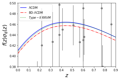
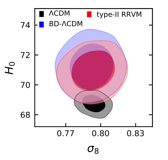
As pointed out above, the BD-CDM model mimics the type-II RVM (cf. Sec. VII.5.11), and hence it is perceived from the GR perspective as a running vacuum model with a (very) mild dynamical gravitational coupling SolaPeracaula:2018dsw ; deCruzPerez:2018cjx ; Sola:2020lba . The effective RVM-behaviour of the BD-CDM can be made apparent if one writes the Friedmann and pressure equations in GR-like fashion, from which one can identify the characteristic RVM form of the vacuum energy density: , with and constants and tracking the departure of the effective gravitational coupling from the local value Sola:2020lba . In Refs. Sola:2019jek ; Sola:2020lba it is shown that the effective EoS of the combined fluid of and usual vacuum energy mimics quintessence at more than CL. This feature could be the smoking gun signaling the departure from GR.
A Word of Caution.
Using Horndeski models to address the and/or tensions comes with a significant caveat, however. The general form of the Lagrangian may be strongly constrained by requiring that the ensuing equation of motion admits a well-posed initial value formulation. In the strongly coupled regime, this issue was studied in Papallo:2017qvl , while the weakly coupled regime was considered in Ref. Kovacs:2020ywu . In the latter, some examples of loss of uniqueness through shock formation and evolution with change in character of the equation of motion (from hyperbolic to elliptic through a parabolic stage) were presented in Bernard:2019fjb .
VII.6.4 Quantum Conformal Anomaly Effective Theory and Dynamical Vacuum Energy
Classical General Relativity receives corrections from the quantum fluctuations of massless conformal fields, through the conformal trace anomaly of the energy-momentum tensor in curved space Duff:1977ay ; Birrell:1982ix
| (94) |
This leads to additional gravitational interactions at macroscopic distance scales Mottola:2006ew ; Giannotti:2008cv ; Mottola:2010gp ; Mottola:2011ud , as becomes clear from the local form of the effective action of the conformal anomaly,
| (95) |
in terms of an additional weakly coupled long range scalar field Antoniadis:1991fa ; Mazur:2001aa ; Mottola:2010gp ; Mottola:2016mpl ; Coriano:2017mux . This ”conformalon” scalar allows vacuum energy to change, leading to a dynamical cosmological dark energy, with potentially observable effects imprinted in the CMB, GWs, and the growth of Large Scale Structure (LSS) Antoniadis:1996dj ; Antoniadis:2006wq ; Mottola:2011ud ; Antoniadis:2011ib .
Specifically, by recognizing that the linear coupling in the anomaly action involves the topological Euler density , and , both of which are total derivatives, naturally defines a -form Abelian potential . Hence its linear coupling to the scalar in (95) can be written
| (96) |
by an integration by parts. The totally anti-symmetric tensor is the -form field strength corresponding to . If the ”Maxwell” term
| (97) |
for this field strength is added to the effective action, where is a coupling constant with dimensions of mass, then the ”Maxwell” equation in the absence of any sources implies that is a constant. Since the stress-tensor for this constant -form Maxwell field matched to the number of spacetime dimensions is , (97) is entirely equivalent to the addition of a positive cosmological constant term to the classical Einstein-Hilbert action Aurilia:1978qs ; Brown:1988kg ; Aurilia:2004cb –in the absence of sources.
With the coupling (96) from the anomaly, the Maxwell eq. acquires a source, and becomes
| (98) |
with the derivative of the scalar conformalon acting as current source. Hence const, and the value of the cosmological ”constant” vacuum energy, determined by the value of can change as the scalar field does.
This effective field theory of the conformal anomaly (95) coupled to the -form potential and -form Maxwell field strength term is different from either scalar-tensor theories, or other modified gravity theories of the Hordenski type, but is well-founded on fundamental quantum field theory principles. The fluctuations of can lead to the scale invariance of the CMB being promoted to full conformal invariance, with the implication of a well-defined non-Gaussian bispectrum differing from slow roll single field inflation models Antoniadis:1996dj ; Antoniadis:2011ib .
The scalar also couples to the conformal part of the metric and leads to scalar ”breather” mode polarization GWs, which should be produced in the early Universe Mottola:2016mpl . Since the vacuum energy can vary in general in both space and time, this effective theory also allows the possibility of spatially inhomogenous non-FLRW cosmologies. A detailed study of dynamical dark energy based on this theory is now just beginning, in order to derive and test its predictions against the trove of LSS and other observational data expected in this decade.
VII.6.5 Ultra-Late Time Gravitational Transitions
The extremely tight constraints on the form of in the range Lemos:2018smw ; Efstathiou:2020wxn combined with the local measurement of , namely Riess:2009pu , which is inconsistent with the CMB constraint Planck:2018vyg implies that a possible transition event may have taken place either just before , see Sec. VII.4, or just after (gravitational transition Marra:2021fvf ). Such a transition event would leave intact the standard model physics in the range while introducing new physics before or after this redshift (time) range. In this subsection we briefly describe the latter possibility.
The absolute luminosity of SNIa may be calibrated using two distinct independent calibrators:
-
1.
The sound horizon at recombination () used as a standard ruler to set the scale for the CDM and thus the SNIa absolute magnitude Camarena:2019rmj ; Camarena:2021jlr and luminosity (inverse distance ladder approach).
-
2.
The locally calibrated standard candles like Cepheid stars which measure the distance to SNIa host galaxies at low redshifts (, Mpc) and thus calibrate the absolute luminosity and magnitude () of SNIa leading to the best fit value Riess:2009pu (distance ladder approach).
The two approaches lead to values of the SNIa absolute magnitude that are inconsistent at a level more than with Camarena:2021jlr . This inconsistency is the basis of the Hubble tension because the difference in the values of is easily translated to a difference in the values of the Hubble constant, since and are degenerate Perivolaropoulos:2021bds ; Theodoropoulos:2021hkk (observable for using SNIa):
| (99) |
which implies that a shift of of
| (100) |
is needed for a decrease of the locally (SNIa) measured by about and thus a resolution of the Hubble tension.
The two measurements of however (CMB sound horizon and local calibrators/SNIa) are performed at different redshift ranges: the Cepheid measurement is performed at where Cepheids and other local distance calibrators are detectable while the measurement using the sound horizon is performed at where the Hubble flow and the CDM are applicable. Thus, the two measurements can be made consistent if a fundamental physics transition changes the SNIa absolute luminosity (or equivalently ) at a redshift Marra:2021fvf .
An abrupt step-like shift of Newton’s constant in the context of a gravitational spatial or temporal transition could play the role of the required fundamental physics transition Alestas:2020zol ; Marra:2021fvf ; Alestas:2021luu . In this context we have
| (101) |
where is the locally measured Newton’s constant. A very recent false vacuum decay Coleman:1977py ; Callan:1977pt ; Patwardhan:2014iha in the context of a scalar tensor theory Lee:2006vka with vacua energy scale eV and with the present horizon scale would naturally produce true vacuum bubbles on scales of Perivolaropoulos:2021bds
| (102) |
Thus, if we were inside such a true vacuum bubble we would observe a transition of at a distance of about Mpc. Surprisingly, such a transition is consistent with current constraints Uzan:2010pm ; PhysRev.73.801 (which constrain mainly the time derivative of and much less a abrupt transition). In fact, hints for such a transition have recently been pointed out in Cepheid Perivolaropoulos:2021bds ; Mortsell:2021nzg and Tully-Fisher data Alestas:2021nmi . It has also been shown that such a transition is consistent with the observed number of galaxies per redshift bin in low redshift galaxy surveys Alestas:2022xxm .
Assuming a SNIa absolute luminosity Amendola:1999vu ; Garcia-Berro:1999cwy , where is a parameter determined by the detailed physics of SNIa explosions, it is found that the required transition of is connected with a gravitational transition of as
| (103) |
where and are the CMB-calibrated and Cepheid-calibrated SNIa absolute luminosities, respectively. Since the Chandrasekhar mass , which plays a crucial role in the SNIa explosion, is , it is clear that the simplest assumption is that which leads to . In the context of this simplest generic assumption we have
| (104) |
which is marginally consistent with current constraints on a possible transition of the Newton constant and implies the presence of weaker gravity by about at times earlier than the transition time corresponding to . Such weaker gravity would lead to weaker growth rate of cosmological matter fluctuations according to the dynamical linear growth equation Skara:2019usd ; Kazantzidis:2018rnb ; Kazantzidis:2019dvk :
| (105) |
where a prime denotes a derivative with respect to redshift . In fact, a reduction of would fit the same data with a 10% larger value for . In the context of a gravitational transition with a CDM background , RSD and WL data are well fit by DES:2017rfo ; Skara:2019usd ; Alestas:2020mvb
| (106) |
which implies when setting Planck:2018vyg and leads to a mechanism for the resolution of the growth tension.
An ultra-late gravitational transition could also have implications on geo-chronology and solar-system chronology addressing corresponding long standing puzzles. For example observational evidence from terrestrial and lunar cratering rates indicates that the impact flux of kilometer sized objects increased by at least a factor of 2 over that last Myrs compared to the long term average Alestas:2021luu . It has been demonstrated that such an increase could be explained in the context of the ultra-late gravitational transition required for the resolution of the Hubble and tensions.
VII.7 Specific Solutions Assuming FLRW
In this subsection, we list some specific solutions of interest to the community that cannot be classified in the previous sections, whether because they are broad enough to enclose very different scenarios, or they simply have an impact along the whole cosmic history. We refer the reader to the more complete review DiValentino:2021izs or the original papers for a more detailed discussion of proposed solutions of the Hubble tension in: inflationary models Tram:2016rcw ; DiValentino:2016ziq ; Rodrigues:2020dod ; Rodrigues:2021txa , self-interacting dark matter Binder:2017lkj , Über-gravity Khosravi:2017hfi , Nonlocal gravity Belgacem:2017cqo , Modified Gravity Lin:2018nxe ; Benetti:2018zhv , unified fluid Yang:2019jwn , quintessential models DiValentino:2019exe , screened fifth forces Desmond:2019ygn , Generalized Chaplygin gas models Yang:2019nhz ; Benetti:2021div ; Benetti:2019lxu ; Salahedin:2020emw , Viscous Generalized Chaplygin gas Hernandez-Almada:2021osl , addition of extra SNIa systematic uncertainties with a varying DE Martinelli:2019krf , metastable DE Shafieloo:2016bpk ; Li:2019san ; Yang:2020zuk , Super-CDM Adhikari:2019fvb ; Adhikari:2022moo , DM-photon coupling Yadav:2019jio , Local Inhomogeneity Kasai:2019yqn , Interaction in the anisotropic Universe Amirhashchi:2020qep , Heisenberg uncertainty Capozziello:2020nyq ; Spallicci:2021kye , Enhanced Early gravity model Zumalacarregui:2020cjh ; Joudaki:2020shz , CMB monopole temperature Ivanov:2020mfr , Decaying Ultralight Scalar Gonzalez:2020fdy , Decaying coupled fermions Benisty:2019pxb , Early mass varying neutrino DE Gogoi:2020qif , Neutrino-majoron interactions Escudero:2019gvw ; EscuderoAbenza:2020egd ; Escudero:2021rfi , Light gravitino scenarios Choi:2019jck , Degenerate decaying fermion DM Choi:2020tqp , Lifshitz cosmology Berechya:2020vcy , a frame dependent, scale invariant DE Adler:2019fnp , light gravitino dark matter with a small non-thermal fraction Gu:2020ozv , cosmology with a Bianchi type-I metric Akarsu:2019pwn , Finslerian models Wang:2018est , Dark Energy model from Generalized Proca Theory Geng:2021jso , Axi-Higgs Universe Fung:2021fcj ; Luu:2021yhl , transitional dark energy Zhou:2021xov , interaction between dark matter and the baryonic component in a modified gravity scenario Adil:2021zxp , Minimal Theory of Massive Gravity deAraujo:2021cnd , Bound Dark Energy delaMacorra:2021hoh , Chameleon Early Dark Energy Karwal:2021vpk , interacting dark energy axions Mawas:2021tdx , the mirror twin Higgs model Bansal:2021dfh , Milgromian gravity Banik:2021woo , a quantum origin for the DE Belgacem:2021ieb , Emergent DE from unparticles Artymowski:2020zwy ; Artymowski:2021fkw , General Relativistic Entropic Acceleration theory Arjona:2021uxs .
VII.7.1 Active and Sterile Neutrinos
The existence of massive neutrinos (either active or sterile) has been confirmed by various observational surveys KamLAND:2004mhv ; Super-Kamiokande:2005mbp ; KamLAND:2008dgz and their presence can affect the cosmological parameters (see Refs. Lesgourgues:2006nd ; Conrad:2013mka for more discussions on the massive neutrinos). According to the observational surveys, the sum of the active neutrino masses, , must be at least eV Gonzalez-Garcia:2012hef . Additionally, some observational experiments indicate that there could be a sterile neutrino which does not interact with the standard model Conrad:2013mka , but it still contributes a mass and in a model dependent way, an increase in the total number of effective relativistic degrees of freedom, . It has been found that the active and sterile neutrinos in the Universe sector can be effective to alleviate the tension Battye:2013xqa ; Boehringer:2016bzy . A Pseudo-Dirac sterile neutrino has been instead proposed as a model to alleviate the Hubble tension in Ref Chao:2021grp , as well as an extended parameter space with ground-based CMB data and a total active neutrino mass different from zero DiValentino:2021imh .
VII.7.2 Cannibal Dark Matter
Cannibalistic dark matter models were initially proposed by Refs. Dolgov:1980uu ; Carlson:1992fn ; Dolgov:2017ujf in the context of general self-interacting dark matter Dolgov:1995rm ; deLaix:1995vi ; Machacek:1994abc . Such models have received a resurgence of interest within the last decade Hochberg:2014kqa ; Kuflik:2016abc ; Pappadopulo:2016pkp ; Farina:2016llk ; Erickcek:2020wzd given their promising ability to impact both the small-scale crisis Spergel:1999mh ; deBlok:2009sp ; Boylan-Kolchin:2011qkt ; Salucci:2018hqu and the tension Buen-Abad:2018mas ; Heimersheim:2020aoc .
If the Lagrangian of a massive dark matter candidate permits interactions, such as in Refs. Bernal:2015ova ; Chu:2017msm ; Bernal:2018hjm ; Heeba:2018wtf , it is possible that it exhibits a cannibalistic behavior. When the species’ thermal energy is high compared to its mass, both the and interactions will be balanced, and the dark matter will behave as an ordinary relativistic species. However, as the species cools and the thermal energy becomes insufficient to overcome the mass gap inherent in the interaction, a cannibalistic phase begins, in which the mass energy of particles is converted through an efficient interaction into thermal energy. As soon as the interaction freezes out (when the number density is sufficiently diluted due to the expansion of the Universe), the species continues to behave like ordinary cold dark matter. In its cannibalistic regime the species is close to (but not quite) relativistic for an extended time, allowing the species to keep a large Jeans scale (suppressing growth on small scales) while avoiding coupling to other relativistic species through the Einstein equations (and thus impacting CMB observables). As such, the cosmological evolution is very similar to that of warm dark matter, except for the intermediate cannibalistic phase, which allows the model to have a reduced impact on the CMB while still strongly suppressing the power spectrum.
While the initial investigations Buen-Abad:2018mas ; Heimersheim:2020aoc in terms of cosmological evolution have shown a promising parameter region, more work is required both at the level of theoretical modeling and complimentary experimental constraints. In particular, joint investigations of constraints from CMB, weak lensing, Ly- data, and/or small scale probes of clustering would be required to further investigate the validity of this model.
VII.7.3 Decaying Dark Matter
The CDM model postulates the additional form of Dark Matter (DM) which clusters gravitationally but is (almost) immune to other interactions. The nature of DM remains elusive so far. From a theoretical point of view, DM can be easily multi-component itself.222222Idea of multi-component DM is inspired by the apparent complexity of the ”visible” sector. For instance, the current cosmological data resolve at least three different components: photons, neutrinos, and baryons. It seems to be natural that DM which dominates the matter content of the Universe also consists of several different species.
One interesting approach that provides a composite content of DM is decaying DM (dDM).232323Not to be confused with the ”Dynamical Dark Matter” (DDM) model discussed in Sec. VII.7.4. The motivation of this scenario arises in purely theoretical considerations Ibarra:2013cra , it also can explain some interesting experimental results Ibarra:2013zia ; Cirelli:2012ut ; Anchordoqui:2015lqa ; Lovell:2014lea ; Iakubovskyi:2014yxa and address the small-scale problems of the cold DM paradigm Wang:2014ina ; Cheng:2015dga . The decaying DM model was developed in the 1980s Flores:1986jn ; Doroshkevich:1989bf and has recently gained renewed interest because of the appearance of persistent tensions between low-redshift measurements and predictions of the CDM cosmology.
There exist several varieties of the decaying DM proposal. DM can be a single unstable component decaying into invisible radiation with a lifetime exceeding the age of the Universe Audren:2014bca . This scenario was suggested as a resolution of the tension, however, the current cosmological data is not constraining enough to unambiguously favor a non-zero DM decay rate Enqvist:2015ara . Alternatively, the unstable DM may decay to the massive particles and invisible radiation at late times Aoyama:2014tga ; DelNobile:2015bqo or even undergo a many-body decay Blackadder:2014wpa ; Blackadder:2015uta . However, this decaying DM scenario is unlikely to alleviate the -tension Haridasu:2020xaa ; DES:2020mpv .242424The somewhat related model in which self-interacting dark matter may be converted into a non-interacting form of radiation with rate proportional to the cosmic expansion Bjaelde:2012wi ; Pandey:2019plg is also disfavored by data Liu:2021mkv . More progress towards reconciling discrepancies between different cosmological measurements can be achieved if one assumes an earlier decay of the DM constituents.
In Ref. Berezhiani:2015yta it was argued that the subdominant DM component decaying after recombination may alleviate the cosmological tensions. This decaying DM setup has two extra parameters with respect to the CDM scenario – a fraction of decaying component in the total DM abundance, where denotes initial densities of decaying and cold DM components, and its inverse lifetime, or width, . The background dynamics for unstable DM () and dark radiation () abundances is driven by
| (107) | |||||
| (108) |
A slightly reduced matter content in the late Universe helps accommodate a low in full accordance with local probes of Large Scale Structure (LSS). Remarkably, the downward shift in the total matter density must be accompanied by the upward shift of to keep the angular acoustic scale of the CMB intact. However, the lack of DM at low redshifts reduces the power of the CMB lensing effect which is in odds with the Planck observations. Thus, the CMB data alone put the stringent limits on this proposal, Chudaykin:2016yfk ; Poulin:2016nat from the Planck 2015 data and Nygaard:2020sow using the newest Planck 2018 likelihood. Including the BAO measurements from BOSS DR12 induces even tighter constraints on the decaying DM fraction by a factor of Chudaykin:2017ptd ; Nygaard:2020sow .
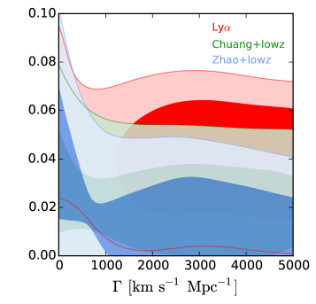
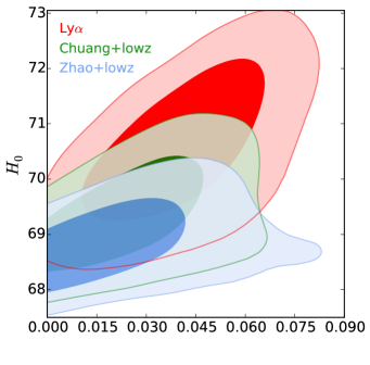
Corresponding constraints in the and subspaces for a different choice of large-scale structure data are shown in Fig. 11. Since a full resolution of the Hubble tension requires Berezhiani:2015yta the CMB and BAO analysis makes the decaying DM solution of -tension increasingly unlikely. The main culprit of these strong constraints is a so-called ”lensing-like anomaly” in the Planck data that over-predicts the CMB lensing signal Planck:2016tof ; Planck:2018vyg and thus strongly disfavors the decaying DM solution which, in turn, favors a weaker lensing effect. In this regard, it is curious to see what fraction of decaying DM is available upon marginalizing over the lensing information in the Planck power spectra. By allowing the CMB lensing power amplitude to be a free fitting parameter, the CMB and BAO data along with the Planck cluster counts and SH0ES measurement yield Chudaykin:2017ptd . Overall, this analysis indicates a mild preference in favor of the decaying DM scenario over CDM Chudaykin:2017ptd . Therefore, before making strong conclusions it has to be understood first why the CDM prediction is in tension with the Planck CMB lensing effect.
One way to mitigate the tight CMB constraints is to assume a short-lived decaying DM component which decays before recombination. Recent investigations Poulin:2016nat ; Nygaard:2020sow reveal interesting implementations of the subdominant unstable component of DM decaying between matter-radiation equality and recombination epochs. The tight Planck constraints on in this case can be significantly alleviated Poulin:2016nat ; Nygaard:2020sow . Moreover, a decay near matter-radiation equality reduces the sound horizon at the drag epoch, , alleviating the tensions with the late-time model-independent probes of , see Ref. Bernal:2016gxb . However, the Hubble tension in this scenario is only marginally alleviated Poulin:2016nat ; Nygaard:2020sow . Like an EDE proposal, in the short-lived decaying DM model, the growth of both metric and density perturbations is amplified that exacerbates (although weakly) the tension.
It was recently proposed that a fraction of DM particles which decay into a much lighter stable relic and photon can solve the long-standing Lithium problem DiBari:2013dna . The electromagnetic injection in the specific energy range would destroy enough Lithium without affecting the abundance of other elements. Since the light decay products act as dark radiation in the early Universe, this scenario was also suggested to alleviate the tension Alcaniz:2019kah . However, this proposal is tightly constrained by the Planck data Anchordoqui:2020djl . Model-independent constraints from BBN on unstable DM which decay into photons and/or electron-positron pairs are provided in Ref. Depta:2020zbh .
Overall, the totality of the cosmological data put tight constraints on the decaying DM scenario as a resolution of and tensions although a few percent decaying DM fraction is still allowable Chudaykin:2017ptd ; Nygaard:2020sow . For models with a subdominant component of DM decaying between recombination and the present epoch, the understanding of the ”lensing-like anomaly” in the Planck data is highly warranted because this feature is responsible for stringent CMB limits on this proposal. To conclude, the current and tensions require either a different (and possibly major) alteration of the CDM model, or derives from some yet unknown systematic effect.
The cosmological scenarios where the heavier particles decay to lighter and invisible radiation are argued to weaken the tension Aoyama:2014tga ; Enqvist:2015ara ; Abellan:2020pmw . These scenarios also relax the tension of CDM predictions with observation of structures at small scales Wang:2014ina ; Cheng:2015dga and can elucidate the origin of high-energy neutrino IceCube events Anchordoqui:2015lqa ; Anchordoqui:2021dls . Ultrahigh-energy cosmic ray experiments could be powerful probes of dDM models in which DM couples to the SM sector Anchordoqui:2018qom .
VII.7.4 Dynamical Dark Matter
Although many models of decaying DM transcend the canonical WIMP or axion frameworks and involve new regions of the DM parameter space, perhaps none do so as dramatically as those that arise within the Dynamical Dark Matter (DDM) framework. The basic idea behind DDM is relatively simple Dienes:2011ja . Rather than focus on one or more stable DM particles, the DDM framework is built on the proposition that the DM in the Universe comprises a vast ensemble of interacting fields with a variety of different masses, mixings, and cosmological abundances. Moreover, rather than imposing the stability for each field individually, the DDM framework recognizes that the decay of a DM component in the early Universe is not ruled out if the cosmological abundance of that component is sufficiently small at the time of its decay. The phenomenological viability of the DDM framework therefore requires that those states within the ensemble with larger masses and SM decay widths have correspondingly smaller relic abundances, and vice versa.
In other words, DM stability is not an absolute requirement in the DDM framework, but is replaced by a balancing of lifetimes against cosmological abundances across the entire ensemble. As a result, individual constituents of the DDM ensemble are decaying throughout the evolution of the Universe, from early times until late times and even today. This leads to a highly dynamical scenario in which cosmological quantities such as the total DM abundance experience a non-trivial time dependence beyond those normally associated with cosmological expansion.
Many extensions to the SM give rise to large ensembles of dark states in which such a balancing naturally occurs. Moreover, because the DM ”candidate” in this framework consists of a carefully balanced DDM ensemble which cannot be characterized in terms of a single well-defined mass, decay width, or interaction cross section, this framework gives rise to many striking experimental and observational signatures which transcend those usually associated with DM and which ultimately reflect the collective behavior of the entire DDM ensemble.
The DDM framework was originally introduced in Ref. Dienes:2011ja , while in Refs. Dienes:2011sa ; Dienes:2012jb explicit DDM models were constructed which satisfy all known collider, astrophysical, and cosmological constraints. Since then, a considerable body of work has focused on various aspects of the DDM framework. One major direction of research consists of analyzing the various signatures by which this framework might be experimentally tested and constrained. These include unique DDM signatures at direct-detection experiments Dienes:2012cf , at indirect-detection experiments Dienes:2013lxa ; Boddy:2016fds ; Boddy:2016hbp , and at colliders Dienes:2012yz ; Dienes:2014bka ; Curtin:2018ees ; Dienes:2019krh ; Dienes:2021cxr .
Indeed, such DDM scenarios also give rise to enhanced complementarity relations Dienes:2014via ; Dienes:2017ylr between different types of experimental probes. Moreover, the non-minimal dark sectors which are the cornerstone of the DDM framework can also lead to observable imprints across the cosmological timeline, stretching from structure formation Dienes:2020bmn ; Dienes:2021itb all the way to late-time supernova recession data Desai:2019pvs and unexpected implications for evaluating Ly- constraints Dienes:2021cxp . Such dark sectors also give rise to new theoretical possibilities for stable mixed-component cosmological eras and a potential re-examination of the age of the Universe Dienes:2021woi .
The second direction of DDM research over the past decade has focused on the numerous ways in which suitably-balanced DDM ensembles i.e., ensembles of dark states in which the widths for decays into SM states are naturally inversely balanced against cosmological abundances emerge naturally within various models of BSM physics. These include theories involving large extra dimensions, both flat Dienes:2011ja ; Dienes:2011sa and warped Buyukdag:2019lhh ; theories involving strongly-coupled hidden sectors Dienes:2016vei ; Buyukdag:2019lhh ; theories involving large spontaneously-broken symmetry groups Dienes:2016kgc ; and even string theories Dienes:2016vei .
Indeed, the dark states within these different realizations can accrue suitable cosmological abundances in a variety of ways, including not only through non-thermal generation mechanisms such as misalignment production Dienes:2011ja ; Dienes:2011sa but also through thermal mechanisms such as freeze-out Dienes:2017zjq . Mass-generating phase transitions in the early Universe can also endow collections of such states with non-trivial cosmological abundances Dienes:2015bka ; Dienes:2016zfr ; Dienes:2016mte .
In general, the mass spectra and corresponding lifetimes and abundances of the individual states within the DDM ensemble turn out to be tied together through scaling relations involving only a few scaling exponents. This is reviewed, for example, in Sect. III of Ref. Curtin:2018ees . The particular physical scenario that one has in mind within the DDM framework then determines these scaling exponents. As a result, the DDM ensemble is described by only a few free parameters, rendering the DDM framework every bit as constrained and predictive as more traditional dark-matter scenarios.
DDM scenarios in which the constituents decay entirely within the dark sector — i.e., to final states comprising other, lighter ensemble constituents and/or dark radiation — are particularly challenging to probe and constrain. Nevertheless, there exist observational handles that can be used to probe and constrain DDM ensembles which decay primarily via ”dark-to-dark” decay processes of this sort, and thus potentially permit us to distinguish them from traditional DM candidates.
For example, dark-to-dark decays of this sort modify the way in which the expansion rate of the Universe, as described by the Hubble parameter , evolves with redshift. These modifications, in turn, affect the functional relationship between the redshifts and luminosity distances of Type-Ia supernovae. In Ref. Desai:2019pvs , constraints based on the observed relationship between the redshifts and luminosity distances of Type-Ia supernovae within the combined Pantheon sample Pan-STARRS1:2017jku were derived for DDM ensembles whose constituents decay via a two-body process of the form , where is a massless dark-radiation field. A partial summary of these constraints is provided in Fig. 12.
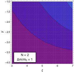
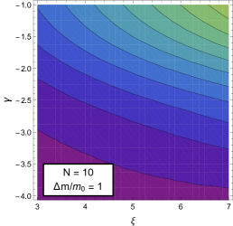
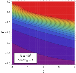

Since the dark-to-dark decays of a DDM ensemble alter the dependence of on , the DDM framework can potentially also provide a way of addressing the tension. In this regard, the advantage of a DDM ensemble relative to a single decaying dark-matter species is that the timescale across which the decays have a significant impact on the expansion rate can be far broader. Nevertheless, the depletion of the overall DM abundance at late times due to decays leads to a suppression of the CMB lensing effect and therefore to tension with Planck data just as it does in other late-time decaying DM scenarios Chudaykin:2016yfk . DDM scenarios in which the decay directly into dark radiation are significantly constrained Anchordoqui:2022gmw .
By contrast, scenarios in which the decays primarily via intra-ensemble processes – e.g., of the form , where once again denotes a dark-radiation field – are more promising Anchordoqui:2020djl ; Anchordoqui:2022gmw . Such decays endow the final-state with non-negligible velocities, thereby modifying the equation of state for each ensemble constituent and modifying the DM velocity distribution of the ensemble as a whole. Moreover, complementary scattering processes of the form through which the different ensemble constituents interact with the dark radiation could potentially also help to ameliorate the tension in the same way that they do in partially acoustic DM scenarios Chacko:2016kgg .
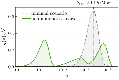
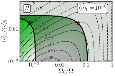
In this connection, it is also worth noting that it is not merely the value of alone, but rather the detailed dependence of the amplitude of matter-density perturbations across a broad range of wavenumbers, which provides an observational handle on DM scenarios with non-cold DM velocity distributions . In such scenarios, free-streaming effects lead to a suppression of cosmic structure on small scales. For DM models such which yield relatively simple, unimodal forms for at all , assessing the impact of these effects on is comparatively straightforward.
By contrast, in the context of non-minimal dark-sector scenarios wherein a significant fraction of the dark-matter abundance is produced non-thermally (e.g., from particle decays) and wherein can be highly non-trivial and even multi-modal, the impact of free-streaming on small-scale structure is more complicated Konig:2016dzg ; Heeck:2017xbu ; Dienes:2020bmn ; Du:2021jcj ; Decant:2021mhj . For example, standard ”recasting” procedures Konig:2016dzg ; Murgia:2017lwo employed in deriving constraints on from Ly--forest data can become unreliable for velocity distributions of this sort. A study of the performance of these recasts for general dark-matter velocity distributions was performed in Ref. Dienes:2021cxp . Results from a study of this sort are shown in Fig. 13.
On the other hand, there exist methods Dienes:2020bmn which permit one to reconstruct the detailed shape of solely from information contained within the linear matter power spectrum — methods which are applicable even when that shape is highly non-trivial. In cases in which differs from the matter power spectrum for CDM primarily due to free-streaming effects, these methods are quite robust in their applicability and are capable of reconstructing the DM velocity distribution with impressive fidelity. By contrast, the situation becomes more subtle in cases wherein the growth of density perturbations at late times is affected by additional complications — such as decays of the after last scattering and/or dark acoustic oscillations Cyr-Racine:2013fsa of the sort which would arise from non-negligible interactions between and the . Nevertheless, the relationship between small-scale structure and the dark-matter velocity distribution can provide a valuable cross-check on cosmological models of this sort.
VII.7.5 Extended Parameter Spaces Involving
Extended cosmological scenarios beyond the 6-parameter CDM model including the parameter free to vary have been widely investigated in the literature, showing that when as preferred by the Planck data, see the discussion in Sec. VI.1, the tension disappears DiValentino:2015ola ; DiValentino:2016hlg ; DiValentino:2017zyq ; DiValentino:2018gcu ; DiValentino:2019dzu ; Benisty:2020kdt ; DiValentino:2020hov . This could suggest a possible systematic error present in the Planck data not accounted for, that is producing the disagreement with the weak lensing and cluster counts measurements. Once the data analysis of the CMB data marginalizes over this phenomenological parameter, the agreement between the parameter obtained by the Planck data and the low redshift measurements is restored.
VII.7.6 Cosmological Scenario with Features in the Primordial Power Spectrum
In Hazra:2018opk without considering any extension to the standard model at the background level, authors project the effect of the differences in the values of the key cosmological parameters to the form of the primordial power spectrum (PPS). In order to realize this task, they did uncover the form of the primordial spectrum by implementing the Modified Richardson-Lucy algorithm (MRL) Shafieloo:2003gf ; Shafieloo:2006hs ; Nicholson:2009pi ; Hazra:2013xva ; Hazra:2014jwa that would fit the Planck temperature data as good as the case of the concordance CDM model, but with a Hubble constant consistent with local measurements, as well as improving the consistency between the derived and parameters with estimations of the weak lensing surveys. Recently there have been more progress in this line to address various tensions by a featured form of the primordial spectrum Hazra:2022rdl . In this context, Antony:2022ert introduces examples of single field inflationary trajectories beyond the slow-roll regime that provides improvements in the Planck data compared to the standard model – partially mimics the effect of unphysical excess lensing and closed Universe. This model simultaneously prefers a higher and lower – a trend that is enhanced with the addition of data from the SH0ES measurements.
Furthermore and in Ref. Keeley:2020rmo authors did explore a class of primordial spectra that can fit the observed cosmic microwave background data well and that could result in a larger value for the Hubble parameter consistent with the local measurements. This class of spectra consists of a continuous deformation between the power law primordial spectrum and the reconstructions from the MRL deconvolution algorithm. More works are needed to assign significance to such features and seek for possible theoretical implementation from inflation Snowmass2021:Inflation . Testing such a form of the primordial spectrum as initial conditions against other cosmological observations would be another important task in this direction.
VII.7.7 Interacting Dark Matter
Several models of interacting dark matter feature a suppression of the matter power spectrum. Some of these models have a cosmologically relevant suppression impacting the tension even after taking into account constraints from the CMB. In particular, dark matter interactions with photons or neutrinos Ali-Haimoud:2015pwa ; Weiner:2012cb ; Wilkinson:2013kia ; Diacoumis:2018ezi have shown to impact structure formation Boehm:2004th ; Bringmann:2013vra ; Cherry:2014xra ; Boehm:2014vja ; Wilkinson:2014ksa ; DiValentino:2017oaw ; Olivares-DelCampo:2017feq ; Escudero:2018thh ; Kumar:2018yhh ; Stadler:2018jin ; Stadler:2019dii ; Becker:2020hzj . This is because the small residual interactions introduce a collisional damping on small scales (for which the Fourier modes entered the Hubble horizon early enough to experience significant interactions) that suppresses the power spectrum on these scales. Similarly, interactions with a dark radiation component have also been invoked in the past Cyr-Racine:2013fsa ; Chu:2014lja ; Rossi:2014nea ; Buen-Abad:2015ova ; Schewtschenko:2015rno ; Lesgourgues:2015wza ; Cyr-Racine:2015ihg ; Krall:2017xcw ; Archidiacono:2017slj ; Buen-Abad:2017gxg ; Archidiacono:2019wdp , though these have been found to be more promising in terms of the Hubble tension Lesgourgues:2015wza ; Becker:2020hzj ; Velten:2021cqj . Interacting models and their consequences were considered in several papers reviewed in Wang:2016lxa .
VII.7.8 Quantum Landscape Multiverse
The authors of Refs. Holman:2005ei ; Holman:2005qk ; Mersini-Houghton:2014jha ; Mersini-Houghton:2008eyr showed in 2005 that the mystery of the unlikely origin of our Universe can be answered and derived within the framework of a a larger phase space of initial conditions, by means of quantum cosmology, when the out of equilibrium dynamics of gravitational and matter degrees of freedom is taken into account. It has been initially proposed Mersini-Houghton:2005axz ; Kobakhidze:2004gm ; Mersini-Houghton:2006phg to allow the wavefunction of the Universe to propagate through the stochastic structure of the string theory landscape vacua, by considering the later to be a physical realization of the phase space of initial conditions from which Universes can spring into existence, and thereby derive instead of postulate the probability of the selection of our initial conditions by means of quantum cosmology.
In the second stage, the decoherence among the branches of the wavefunctions was included, thus extending the mini-superspace of three-geometries and landscape moduli fields to include an infinite number of long wavelength fluctuations of space time and of the moduli, which provided the environment and it is sufficiently weakly coupled to the system in order to not interfere with it in process of measurement. Mathematically, this complex system of the wavefunction of the Universe being a functional of an infinite dimensional superspace is similar to known condensed matter systems such as spin glass and quantum dots, and can be solved by means of random matrix theory. Solutions found for the branches of the wavefunction of the Universe Holman:2005ei ; Holman:2005qk ; Mersini-Houghton:2008eyr ; Mersini-Houghton:2014jha revealed that: firstly, a whole family of wavepackets of branches of the wavefunction that settled on high energy vacua on the landscape undergo a similar expansion history like our Universe to transition from a quantum to a classical universe, they survive the backreaction of matter fluctuations (which tries to slow their growth), and therefore have the highest chance of existence, while the ones that settled on low energy vacua cannot survive the backreaction matter and remain quantum particles forever; secondly, since there is a whole family of solutions that survive and grow to classical Universes, then the answer to the question of our high energy cosmic inflation comes at the price of extending our standard model of cosmology to a quantum multiverse framework in which our Universe is embedded and is just a humble member in a vastness.
The attraction of this theory is that for the first time it provided an answer to the problem of our unlikely initial state, and it did so by deriving it from first principles, namely to: why our Universes originate from a high energy low and entropy state? Having a formalism of well trusted quantum equations which allows us to follow consistently a coherent story of evolution of our Universe from before it inflated, when it was just a branch of the wavefunction on some landscape energy vacua, follow it through cosmic inflation, and after it transitions into a large classical Universe, opens a window from which we can glean into the larger structure on which our Universe was embedded, it allows us a way to collect evidence on the multiverse. Until this work, the conventional wisdom was that limited by the speed of light, we cannot test the existence of multiverse and therefore any theory of the multiverse cannot be scientific. Since, the multiverse research has become a mainstream field in cosmology.
In Refs. Holman:2006an ; Holman:2006ny ; Mersini-Houghton:2016jno the authors realized that quantum entanglement and decoherence are two sides of the same coin, and that the backreaction of the long wavelength fluctuations, very weakly coupled to the system being ‘watched’ (our Universe), which triggers decoherence and destroys entanglement among the different branches which becomes decohered Universe, leaves its traces on our CMB sky. The authors proposed to calculate them and thus use quantum entanglement as a way to test this theory and collect evidence for the quantum multiverse in which our Universe is embedded. In two papers named, ”Avatars of the Landscape” in 2005 Holman:2006an ; Holman:2006ny ; Mersini-Houghton:2016jno they derived a series of predictions leftover in our sky from the early quantum origins, including the Cold Spot, a suppressed , a supersymmetry breaking scale which is much higher than the expected tEV scale, a power asymmetry between the two hemispheres, suppressed multipoles at the lowest and so on. Later observations with WMAP and Planck confirmed the existence of these anomalies at exactly the scales and sized that were predicted in Refs. Holman:2006an ; Holman:2006ny ; Mersini-Houghton:2016jno , in the case of the Cold Spot at a significance higher than 4.
The reason for the giant void that shows as a Cold Spot in temperature CMB maps, and the suppressed value of is that the entanglement of our Universe at its infancy with all the other branches of the wavefunction and the backreaction from the collective contribution of long wavelength fluctuations which was calculated in Refs. Holman:2006an ; Holman:2006ny ; Mersini-Houghton:2016jno provided a second source of fluctuations that contributed to CMB in addition to the typical inflationary fluctuations. Since the only scales in this problem are the energy of cosmic inflation and that of SUSY breaking scale, then the model does not allow much tweaking room for fitting data to the model. Therefore in Refs. DiValentino:2018wum ; DiValentino:2016nni ; DiValentino:2016ziq the status of this theory has been checked with the most recent and detailed Planck satellite data and found it is reassuring that the fit of anomalies predicted in the theory continues to be robust.
VII.7.9 Quantum Fisher Cosmology
The aim of Quantum Fisher Cosmology Gomez:2020xdb ; Gomez:2020gqa ; Gomez:2021yhd ; Gomez:2021hbb ; Gomez:2021jcl is to use the quantum Fisher information about pure de Sitter states to derive model independent observational consequences of the existence of a primordial phase of the Universe of de Sitter accelerated expansion. These quantum features are encoded in a scale dependent quantum cosmological tilt that defines what we can call the de Sitter universality class. The experimental predictions are: i) A phase transition from red into blue tilt at a scale order Mpc-1 that naturally solves the cosmological trans-Planckian problem, ii) A spectral index for curvature fluctuations at CMB scales Mpc-1 equal to , iii) A tilt running at scale Mpc-1 equal to , iv) An enhancement of the amplitude of CMB peaks for extremely high multipoles () that can provide a natural mechanism for primordial black hole formation as a source of dark matter, v) A lack of power at scales of Mpc with respect to the CMB scale that can explain the tension.
The key ingredient is the quantum Fisher information associated with the family of de Sitter invariant vacua describing scalar spectators in a pure de Sitter background. These pure states are sometimes denoted, in the literature, as -vacua. What the quantum Fisher information naturally defines is a metric on this set of states. In essence, it measures the quantum distinguishability of different vacua. There exists an extensive literature on both the quantum consistency of vacua as well as on the physical viability of using the Bunch Davis vacuum to define the quantum fluctuations describing the CMB spectrum of fluctuations. Some of these problems are related with the trans-Planckian problem and the computation of one loop effects on these vacua. We will surpass some of these well known difficulties focusing on a well defined quantity associated with the family of vacua, namely the quantum Fisher information associated with this one parameter family of pure states. As stressed before, this quantum information naturally leads to a finite quantum variance for the parameters labeling these vacua. The main message of our work is that this quantum variance can account for the anomalous scale dependence of the cosmological power spectrum normally derived after adding a quasi de Sitter deformation. Moreover, this quantum information encodes the quantum variance of the parameter. The parameter can be associated with a natural energy scale defined as . More precisely with the standard squeezing parameter and with .
The starting point of the quantum Fisher approach to Cosmology is to identify the scale transformations of this quantum Fisher information. In other words, we are interested in identifying how the information controlling the quantum variance of depends on the energy scale at which we are working. The main finding of Gomez:2020xdb ; Gomez:2021yhd ; Gomez:2021jcl is that this scale transformation of the quantum Fisher is anomalous with a scale dependent tilt defined as . This is the tilt depicted in Fig. 14. As discussed in Gomez:2020zev this figure represents the numerical result obtained after evaluating the quantum Fisher information with an IR cutoff on the number of contributing entangled pairs. The sensitivity of the result on this IR cutoff was discussed in Gomez:2020zev .
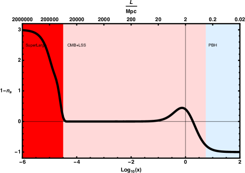
For comoving Lagrangian scales we predict that the value of should be larger than at scales of Mpc, which is where Planck18 measured the tilt. Therefore, there should be a lack of power with respect to the CMB inferred one given by the difference in a power-law power spectrum when adopting the CMB value or the value from Fig. 14 corresponding at these scales (). In more detail:
| (109) |
where we have used that the difference in scales between Planck18 CMB and the weak lensing surveys at Mpc is about a factor 3. Now, from Fig. 14 at the corresponding scale of we see that , so
| (110) |
where as measured from the CMB scale of (to probe scales of 8 Mpc which is where KiDS and SPT report their measurements). This results in . On the other hand the observed ratio . This is in good agreement with our prediction that at small scales the Universe would be less clumpy than the one at CMB scales.
VII.7.10 Quartessence
An interesting class of cosmological models, known as quartessence or unified dark matter, in which and dark matter are considered to be the two faces of the same quantity, can explain the current accelerated expansion of the Universe and also can explain the growth of the large scale structure of the Universe Camera:2017tws . A family of quartessence models can be described by the following Lagrangian Bertacca:2008uf :
| (111) |
where () is a Born-Infeld type kinetic term (Born:1934gh, ) and
| (112) | |||||
| (113) |
in which is a free parameter and . At the background level, these models are indistinguishable from the CDM model. The only free parameter is dependent on the effective sound speed of quartessence, , and for , we have . In fact, the sound speed evolves with redshift as (Bertacca:2008uf, )
| (114) |
where and are respectively the present day values of the density parameter for the effective cosmological constant and dark matter. Note, that for , one recovers the CDM model. For the above model labeled as CDM Camera:2017tws , it has been found that Planck 2015 alone can estimate a very lower value of at 68% CL, which is close to the result from KiDS-450 Kuijken:2015vca ; Hildebrandt:2016iqg ; FenechConti:2016oun ; Joudaki:2016kym , thus resolving the tension completely within .
VII.7.11 Scaling Symmetry and a Mirror Sector
Since the Hubble rate (or rather, its inverse ) sets the total volume of the observable Universe at any given epoch, changing means rescaling the universe’s overall size. It turns out that if such a transformation is accompanied by a rescaling of all other important cosmological distances by the exact same amount, then important observables seen projected on the celestial sphere such as the CMB and LSS (including baryon acoustic oscillation (BAO)) are left entirely unchanged from our perspective. Fundamentally, this symmetry exists because (i) most cosmological data are analyzed in terms of -point angular correlation functions, which are unaffected by the above scaling since angles are invariant under such transformation; (ii) the equations of motion describing the linear evolution of fractional density fluctuations (for photons, baryons, dark matter, etc.) in the Universe only depend on ratios of distances, which are invariant under a rescaling of all length scales in the problem; and (iii) the initial conditions for structure formation in our Universe do not have an intrinsic scale built-in (i.e. their spectrum is a power law), allowing us to rescale the physical size of density fluctuations without changing their amplitude (up to a small harmless correction Zahn:2002rr ).
In the pre-recombination Universe (), there are two important length scales in cosmology: the Hubble length and the photon mean free path , where is the scale factor, is the free electron density, and is the Thomson cross section. Rescaling both quantities by a constant factor (at all times) leaves cosmological observables invariant. Of course, scaling up the Hubble rate implies via the Friedmann equation () that we must increase the energy density of the Universe at all times. To leave the evolution of the gravitational potentials unchanged, the Einstein equations then tell us that this must be done by equally scaling the individual energy densities of all the constituent of the Universe, . In all, Ref. Cyr-Racine:2021alc finds that a broad array of cosmological observables are invariant under the following transformation
| (115) |
for some constant . The third entry in the transformation is necessary to ensure the initial amplitude of fluctuations is unchanged under the transformation. Here, is the amplitude of scalar fluctuations and is the scalar spectral index. The existence of this symmetry opens the doors for the CMB and LSS data to accommodate a larger value of the Hubble constant without necessarily degrading the quality of the fit between model and data, and also leave unchanged.
We emphasize that the above is not another model that could alleviate the Hubble tension, but rather a general paradigm to understand which models can naturally accommodate large Hubble constant values while being automatically consistent with cosmological data. As in much of theoretical physics, the existence of a symmetry broken by different physical effects can lead to key insights about the fundamental origins of the Universe. In our particular case, the scaling symmetry given in Eq. (115) is broken by the COBE/FIRAS measurement of the CMB black body spectrum Fixsen1996 ; fixsen09 , which fixes the energy density of photons today (and thus prohibits us from performing the transformation ). Indirectly, COBE also prohibits us from adding more baryons to the Universe, since the baryon-to-photon ratio is precisely measured by CMB anisotropies. Nevertheless, nothing prevents us from adding dark photons that couples to dark baryons in a similar way to how regular photons couple to standard baryonsAckerman:2008gi ; Feng:2009mn ; Agrawal:2016quu ; Foot:2002iy ; Foot:2003jt ; Foot:2004pa ; Foot:2004wz . Such a mirror dark sector has been studied extensively in the literature since it was long recognized that it could help explain why gravity is so much weaker than other forces in the Standard Model (SM). Could the Hubble tension be revealing the existence of such a mirror sector?
While necessary to evade the COBE/FIRAS bound, the mirror sector does not implement by itself to the second important ingredient of the scaling transformation: the necessary increase of the photon scattering rate (the second entry in Eq. (115)). This is certainly the most challenging aspect of the scaling transformation since it involves SM physics at low energies, which is tightly constrained by a multitude of observations. Ref. Cyr-Racine:2021alc used a phenomenological approach based on varying the primordial helium abundance, which runs into serious constraints from light-element abundance measurements.252525A realistic model of Dark Atoms based on it has been explored in Blinov:2021mdk . A more promising approach likely requires variation of fundamental constants, especially the fine-structure constant and the electron mass. Varying these parameters has shown some promises in alleviating the Hubble tension (see e.g. Refs. Sekiguchi:2020teg ; Hart:2019dxi ; Hart:2021kad ), and the scaling symmetry given above can help us understand why such ideas work well. Another challenge is how to reconcile BBN predictions in the presence of a rescaled Hubble rate with direct abundance measurements.
In all, the scaling symmetry highlights the important role that the photon scattering rates and BBN light-element abundances play in the and tension. It provides a clear target for model builders that, if reached, would guarantee compatibility between CMB, LSS, and local inference of .
VII.7.12 Self-Interacting Neutrinos
The physics of neutrinos is one of the fascinating topics in modern cosmology even though we have been able to extract only a very minimal information about the neutrinos. Recently, it has been observed that the introduction of new physics in the neutrino sector in terms of the interactions between themselves Kreisch:2019yzn ; Lancaster:2017ksf ; Blinov:2019gcj ; Barenboim:2019tux , which is theoretically possible, might be able to offer an appealing route to alleviate the cosmological tensions Kreisch:2019yzn ; Venzor:2022hql . After decoupling from other standard model particles, neutrinos are considered to be freely streaming throughout the Universe, but they can interact with each other or with other cosmic species via their gravitational interactions. This gravitationally influenced interaction could affect the cosmic observables and this may result in interesting consequences, including opening up the inflation parameter space Barenboim:2019tux . In Ref. Kreisch:2019yzn the authors considered a Lagrangian describing the interaction between different neutrino mass eigenstates of the form
| (116) |
where is a left-handed neutrino Majorana spinor, is a (generally complex) coupling matrix in which the indices , labeled the neutrino mass eigenstates. This is a Yukawa-type interaction with a massive scalar and this may arise in the scenarios where neutrinos interact with a Majoron Gelmini:1980re ; Simpson:2016gph ; Berlin:2018ztp . The presence of the interaction in the neutrino sector quantified through the above Lagrangian may delay the onset of neutrino free streaming until close to the matter-radiation equality leading to a higher value of the Hubble constant and a lower value of the matter fluctuations Kreisch:2019yzn .
VII.7.13 Self-Interacting Sterile Neutrinos
The short baseline (SBL) neutrino oscillation experiments Giunti:2019aiy suggest the existence of a fourth sterile neutrino with a eV mass. However, the existence of sterile neutrinos is not compatible with cosmology since they suppress the structure formation of the Universe. This problem can be bypassed if by some unknown mechanism they can be either prevented from thermalizing in the early Universe or removed by subsequent annihilation. Considering such limitation, the authors of Ref. Archidiacono:2014nda suggested a possible revision in the sterile neutrino sector in which the sterile neutrino interacts with a new light pseudoscalar degree of freedom. This proposal got attention in the cosmological community because with such coupling in the sterile neutrino sector, the effective scenario can increase the Hubble constant value and consequently alleviate the Hubble constant tension Archidiacono:2015oma ; Archidiacono:2016kkh ; Archidiacono:2020yey ; Corona:2021qxl .
VII.7.14 Soft Cosmology
In soft cosmology Saridakis:2021qxb ; Saridakis:2021xqy one allows for small deviations from the usual cosmological framework due to the effective appearance of soft-matter properties in the Universe sectors jones2002soft ; sagis2011dynamic . Hence, as a first approach on the subject, one considers that, intrinsically or effectively, dark energy and/or dark matter may have a different EoS at large scales, i.e. at scales entering the Friedmann equations, and a different one at intermediate scales, i.e. at scales entering the perturbation equations. This possible deviation of the large-scale (ls) and intermediate-scale (is) EoS can be quantified by introducing the softness function . Hence, in the simplest scenario one has
| (117) | |||||
| (118) |
where and are the softness parameters for the dark energy and dark matter sectors, respectively. Standard cosmology is recovered for . Thus, although the Friedmann equations are and , where is the equation-of-state parameter of the th sector at large scales, the (linear, scalar, isentropic) perturbation equations in the Newtonian gauge read
| (119) | |||||
| (120) |
where is the density perturbation, the divergence of the fluid velocity, the wavenumber of the Fourier modes, and the effective sound speed square for the th sector which determines the clustering properties, being zero for maximal clustering and one for no clustering.
Soft Dark Energy – As the first soft extension of CDM scenario we consider a model where dark matter is the usual, non-soft, dust one at all scales, while dark energy is the soft component with large-scale behavior that of a cosmological constant. Hence, we impose fixed , namely as in the standard dust dark matter case, while we set and , so that is the only extra free parameter comparing to CDM cosmology. Standard cosmology is recovered for the value . In the left graph of Fig. 15 we depict the as a function of , where we can see alleviation of the tension.
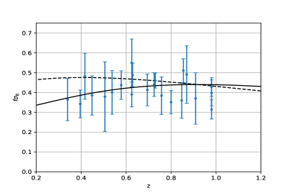
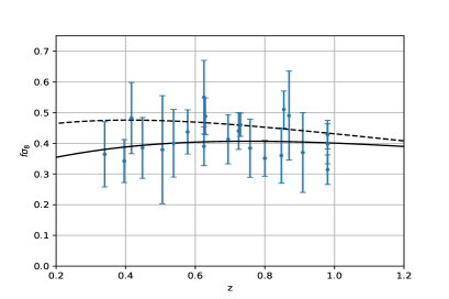
Soft Dark Matter – As another soft extension of CDM scenario we consider a model where dark energy is the usual cosmological constant, with , however dark matter is soft with and , and therefore is the only extra free parameter comparing to CDM cosmology (the latter is recovered for the value ). In the right graph of Fig. 15 we depict the as a function of , where we can see the tension alleviation.
In summary, soft cosmology can alleviate the tension due to the slightly deviated perturbation-level properties it introduces. Finally, we mention that the whole consideration is independent of the underlying gravitational theory, and it can be applied both in the framework of general relativity, as well as in modified theories of gravity in which dark energy sector is of gravitational origin (nevertheless, deviating from general relativity would provide additional possibilities to induce effective soft properties to the dark sectors).
VII.7.15 Two-Body Decaying Cold Dark Matter into Dark Radiation and Warm Dark Matter
One of the solutions proposed to solve the tension is given by a two-body Decaying Cold Dark Matter (dCDM) model where all of the dark matter is assumed to decay into a massless (dark radiation) and a massive warm DM (WDM) species. See Sec. VII.7.3 for alternative models of decaying DM. The phenomenology of such a model has recently been reviewed in great details in Ref. Abellan:2021bpx . The model is characterized by two parameters, the dCDM lifetime, , and the fraction of dCDM rest mass energy transferred to the dark radiation, given by Blackadder:2014wpa
| (121) |
where and denote the mass of the parent particle and massive decay product respectively. Thus, , with the lower limit corresponding to the standard CDM case, so that , and corresponding to DM decaying solely into dark radiation. In general, small values (i.e. heavy massive decay products) and small values (i.e. lifetimes much longer than the age of the Universe) induce little departures from CDM. In the intermediate regime, the velocity-kick received by the warm decay product imprints a characteristic suppression to the matter power spectrum, in a similar fashion as massive neutrinos or warm dark matter. One key difference with respect to these scenarios is the fact that the power suppression is less significant at high redshift, simply because the abundance of the warm decay product is smaller in the past. This allows the model to reduce the value as compared to that inferred from the standard CDM model, while preserving a good fit to CMB, BAO, growth factor and uncalibrated SNIa data. The authors of Ref. Vattis:2019efj suggested that such a model can provide a resolution of the Hubble tension (see also Clark:2020miy ).
However, this conclusion was recently challenged in Refs. Haridasu:2020xaa , where it was shown that including CMB and SNIa data spoils the success of the model to resolve the Hubble tension. Still, in Ref. Abellan:2020pmw , it was shown thanks to a new fluid approximation to describe the perturbations of the massive decay products, that such a model can in fact resolve the tension if Gyr. As discussed in Ref. Abellan:2020pmw , this model could also have interesting implications for model building, the small-scale crisis of CDM and the recent XENON1T excess.
VII.8 Beyond the FLRW Framework
The Hubble constant has a special standing within the class of Friedmann-Lemaître-Robertson-Walker (FLRW) cosmological models, since it arises as an integration constant when one solves the Friedmann equations. As a result, it is generic to all FLRW cosmologies. Now, it is no secret that our local Universe is not an FLRW Universe and that there are well documented flows towards the Shapley supercluster at a distance of approximately Mpc, e.g. Ref. Hoffman:2017ako . In the aftermath of the HST Key project HST:2000azd , it was also recognised that varies across the sky in the local Universe McClure:2007vv . This in itself is unsurprising, since the underlying Hubble flow and the rate of expansion need to be inferred from these averages. Historically, this has been an insanely difficult endeavour and even now disagreements have emerged in the distance ladder between Cepheid Riess:2020fzl and TRGB calibration Freedman:2021ahq .
Recall that the cosmological principle paradigm simply states that the Universe is well modelled as being isotropic and homogeneous at suitably large scales. If one further assumes the decoupling of scales in the underlying metric theory, such that the dynamical theory defined on such large scales is insensitive to the particularities of the regional matter configurations and dynamics, this implies that cosmic structures and their evolution can be ignored altogether at such scales and that the large-scale Universe can be modelled by an FLRW metric. If one stipulates that the large-scale Universe is well described by a homogeneous-isotropic model, one may ask what the scale of transition towards homogeneity and isotropy is? While this statement is vague, one can try to quantify what is meant by ”suitably large scales”, and within the flat CDM model, estimates of Mpc exist Yadav:2010cc as a scale beyond which the fractal dimension of the distribution becomes statistically indistinguishable from that of a perfectly homogeneous and isotropic distribution. The homogeneity scale estimates depend on the statistical measure used. Taking into account all correlation properties in the distribution by employing the Minkowski Functionals Mecke:1994ax the homogeneity scale seems to be even larger Wiegand:2013xfa . There are claims of large structures in the Universe that appear challenging for the hypothesised transition to homogeneity, for example the Sloan Great Wall Gott:2003pf , the Huge Large Quasar Group Clowes:2012pn or the Hercules–Corona Borealis Great Wall Horvath:2015axa . These claims of violations of the cosmological principle have quickly been countered Park:2012dn ; Nadathur:2013mva ; Ukwatta:2015rxa ; Christian:2020den , usually on statistics alone. In short, despite a host of claims, there is little evidence to support any breakdown of the cosmological principle, at least with inhomogeneities.
The strongest observational evidence for an isotropic and homogeneous Universe comes from the CMB. Even to the naked eye, Planck’s maps of micro-Kelvin temperature anisotropies provide a convincing snapshot of a statistically isotropic Universe. The statistically isotropic CMB temperature field is conventionally used as a heuristic argument for modelling the large-scale Universe by an FLRW cosmological model. However, the FLRW model assumption is stronger than that of statistical homogeneity and isotropy; cf. the above discussion. Care must therefore be taken in making rigorous any statements about the underlying metric model based on observations such as the CMB. The CMB photon energy field as viewed by the observer is a quantity which is integrated over scales comparable to the age of the Universe. It is possible that large regional departures from FLRW curvature can be present without breaking of the almost-isotropy of the CMB. Extended versions of the Ehlers-Geren-Sachs theorem 1995ApJ…443….1S ; Rasanen:2009mg that seek to constrain the departures from an FLRW space-time metric based on the level of isotropy of the CMB temperature field within general relativity, must make assumptions on individual components of the covariant derivatives of the energy function for classes of observers to arrive at the conclusion that the Universe is ”almost-FLRW”.262626The original Ehlers-Geren-Sachs theorem Ehlers:1966ad states that the space-time is FLRW or static if the Universe energy-momentum content is a perfectly isotropic radiation fluid around every point. Almost-versions of the theorem are concerned with the realistic scenario of almost-isotropic CMBs as viewed by observers in space-times with realistic energy-momentum content. These components are not directly observable, and are in fact expected to be large in a Universe with large density contrasts Rasanen:2009mg . Thus, even though appealing as an argument for FLRW modeling of the Universe as a whole, almost-isotropy of the CMB does not constitute a proof of the almost-FLRW Universe.
The most notable anisotropy in the CMB is a dipole multipole), the magnitude of which is in the milli-Kelvin range. This dipole is assumed to be a Doppler effect due to relative motion. Obviously, this assumption is a loose end, and now that we find ourselves in a time of crisis, potentially confronted by a discrepancy in , it is prudent to test the assumption that the dipole is purely kinematic in origin. Interestingly, those tests have been pursued over the last two decades, and caveats aside, a consensus has emerged whereby the magnitude of the cosmic dipole inferred from both radio galaxies Blake:2002gx ; Singal:2011dy ; Gibelyou:2012ri ; Rubart:2013tx ; Tiwari:2015tba ; Colin:2017juj ; Bengaly:2017slg ; Siewert:2020krp and quasars Secrest:2020has exceeds the CMB dipole. Similar conclusions have been recently reached by studying the Hubble diagram of Type Ia SN Singal:2021crs and QSOs Singal:2021kuu . This naïvely implies that distant sources are not in the ”CMB frame” and opens up the possibility that the CMB dipole may have been misinterpreted. On the flip side, a recent analysis of the high CMB multipoles is consistent with a kinematic CMB dipole Saha:2021bay (see also Ref. Ferreira:2020aqa ), but the errors are large. Curiously, various CMB anomalies exist (see Ref. Schwarz:2015cma for a review), such as the planar alignment of the quadrupole-octopole deOliveira-Costa:2003utu ; Schwarz:2004gk and the anomalous parity asymmetry Land:2005jq , which may have some origin in the CMB dipole Kim:2010gf ; Naselsky:2011jp . Objectively, if there is no coherence in CMB anomalies, then few conclusions can be drawn. However, if the anomalies have directional dependence, then the plot thickens. Assuming there is a mismatch in the cosmic dipole that can be independently verified by SKAO Bengaly:2018ykb , the simplest and most consequential interpretation is that the Universe is anisotropic. While current data suggests that flat CDM is a good approximation, one can ask how pronounced is any anisotropy, if real? Tellingly, the CMB dipole direction also appears in a documented preferred axis for QSO polarisations Hutsemekers:2000fv ; Hutsemekers:2005iz and scaling relations in galaxy clusters Kaiser:1986ske also point to an anisotropy consistent with the CMB dipole direction Migkas:2020fza ; Migkas:2021zdo . Furthermore, observations of strong lensing time delay Wong:2019kwg ; Millon:2019slk , Pantheon Type Ia SN Pan-STARRS1:2017jku , QSOs standardised through UV-X-ray relation Risaliti:2015zla ; Lusso:2020pdb and GRBs standardised through the Amati relation Amati:2008hq , consistently return higher values of in hemispheres aligned with the CMB dipole direction, at least within the flat CDM model Krishnan:2021dyb ; Krishnan:2021jmh ; Luongo:2021nqh . Obviously, variations of cosmological across the sky with the flat CDM model make any discrepancy between Planck’s determination of with the same model and local determinations a moot point. Given the rich variety of the above observations, and the differences in underlying physics, it is hard to imagine that the CMB dipole direction is not a special direction in the Universe. The status quo of simply assuming that it is kinematic in origin, especially since it is based on little or no observational evidence, may be untenable. If this claim is substantiated, not only do the existing cosmological tensions in and need revision, but so too does virtually all of cosmology. In short, great progress has been made through the cosmological principle, but it is possible that data has reached a requisite precision that the cosmological principle has already become obsolete.
VII.8.1 Cosmological Fitting and Averaging Problems
The cosmological principle stipulates that there is a length scale beyond which the Universe appears as being approximately spatially homogeneous and isotropic. If one further assumes the decoupling of dynamics of volume sections beyond such a scale of homogeneity and isotropy from the local space-time configurations of matter and curvature, this implies the modelling of the large-scale Universe by an FLRW metric model. The CDM framework of cosmology builds on this assumption of decoupling. However, going beyond the CDM framework, one could imagine a Universe which does obey the cosmological principle, but where the regional distributional properties of matter and curvature has importance for the large scale cosmological dynamics.
The problem of taking into account such distributional properties in the large scale modelling of our Universe is sometimes referred to as the cosmological fitting problem Ellis:1984bqf ; Ellis:1987zz . Various approaches to formalising the fitting problem that build on averaging operations of Einstein’s equations have been developed in e.g. Refs. Zalaletdinov:1992cg ; Zalaletdinov:1992cf ; Zalaletdinov:1996aj ; Buchert:1999er ; Buchert:2001sa ; Buchert:2007ik ; Wiltshire:2007jk ; Rasanen:2008be ; Rasanen:2009uw ; Korzynski:2009db ; Gasperini:2009wp ; Gasperini:2009mu ; Buchert:2011sx ; Wiltshire:2011vy ; Gasperini:2011us ; Ben-Dayan:2012uam ; Uzun:2018yes ; Buchert:2019mvq . Within such formalisms, the departure of the large-scale dynamics from that of an FLRW Universe without structure is sometimes denoted cosmological backreaction; see Refs. Green:2014aga ; Buchert:2015iva for a debate on the level of importance of backreaction effects in our Universe.
The Buchert averaging scheme Buchert:1999er ; Buchert:2001sa ; Buchert:2019mvq is the most widespread framework for quantifying backreaction effects; see also Buchert:2022zaa for an extension of the Buchert averaging scheme to the past lightcone of an observer. In this framework, it is made explicit how the large-scale volume evolution is affected by backreaction terms. For instance, in an irrotational dust Universe backreaction in the matter frame is given by variance in expansion rate over volume and regional shearing Buchert:1999er . The backreaction effects can in this case be collected in a single term, which enters in the average dynamical equations for the large-scale volume in such a way that it mimics a dark energy-like effect for large-scale isotropic averages (dominance of expansion variance between voids and matter-dominated regions), but also a dark matter-like effect on smaller scales where the backreaction term can change its sign in cases where anisotropic structures dominate the distribution Buchert:1999er ; Buchert:2007ik . The backreaction term in turn couples to the average spatial Ricci-curvature of the space-time, thus breaking the Friedmann conservation law const, where is the spatial Ricci-curvature and is the scale factor of the FLRW Universe model; see Refs. Buchert:1999er ; Heinesen:2020sre for details.
Backreaction as defined by Buchert Buchert:1999er reduces to a boundary term in Newtonian cosmology Buchert:1995fz ; however, see Ref. Vigneron:2021tpi describing the possibility of volume-integrated backreaction in locally Newtonian theory defined on non-Euclidean topologies, and see also Brunswic:2020bjx for an assessment of topology and GR integral constraints. Non-zero backreaction effects for domains without boundaries defined on non-Euclidean topological structures must thus arise from relativistic effects; see Rasanen:2010wz and references therein. However, such relativistic effects need not be associated with astrophysical structures with large relative speeds or with structures in the ”strong-field” regime,272727See Korzynski:2014nna for an example of an exact GR solution where all of the individual structures are in the ”weak-field” regime, but where the global matter distribution nevertheless exhibits manifestly relativistic effects. in the sense of the Schwarzschild potential , where is the mass and is the radius of the structure. We remark that backreaction effects could arise in Newtonian approximations of general relativity: The small velocity and weak-gravitational potential limit of general relativity is not strictly Newtonian but subject to additional degrees of freedom and constraints Ellis:1994md ; Rainsford:2000ew ; see for instance Ref. Senovilla:1997bw and references therein for examples of Newtonian theories that cannot be recovered in any limit of general relativity. We might further add to the above mentioned subtleties that, even for space-times with negligible backreaction as measured by the backreaction functionals defined in Buchert:1999er ; Buchert:2001sa ; Buchert:2019mvq , observations might exhibit non-negligible departures from any simple FLRW model prediction, depending on the scale of observation and the type of the cosmological measurement. The reverse is also true: it is in principle possible to have space-times where certain backreaction terms are formally large, but where observations are close to an FLRW prediction.
The dynamical differences of the large-scale universal dynamics from that prescribed by a structure-less FLRW model space-time would be a natural candidate for explaining the differences in CDM parameters as inferred from early and late epoch Universe probes. The potential for explaining the Hubble tension with dynamical backreaction effects has been examined within crude analytical approaches Heinesen:2020sre and numerical relativity Macpherson:2018akp , but is far from being an exhausted topic of investigation. The cosmological fitting problem and its significance for Universe observations – including the impact of cosmic structure on the determination of ”background” cosmological parameters such as the Hubble constant – is a rich topic of investigation with many subtleties as indicated in the above review. Regional inhomogeneity and anisotropy and any resulting backreaction effects on the large scale Universe description are appealing possible solutions to the dark energy problem, coincidence problem, and parameter tensions in modern cosmology within the theory of general relativity and without the introduction of additional energy-momentum degrees of freedom. Though any physical backreaction effects must likely arise from subtle departures from strict Newtonian Universe modelling, and is therefore an involved topic of research, it might thus at the same time be argued to be one of the simplest possible solutions to the modern challenges faced in cosmology.
VII.8.2 Data Analysis in an Universe with Structure: Accounting for Regional Inhomogeneity and Anisotropy
In a Universe that contains structures, a spatial invariance with respect to translation and rotation transformations is necessarily broken at some level. As suggested in the above introduction, such symmetry breaking might be more pronounced and important for cosmological inference than is usually accounted for in CDM analysis of data. One way to take into account regional inhomogeneities and anisotropies is to employ exact solutions or perturbative models, a few examples of which are discussed in Sec. VII.8.3. Another option is to remain agnostic about the particularities of the regional properties of the underlying space-time metric.
For this purpose, we might use cosmographic approaches282828The cosmographic frameworks listed here do not assume the FLRW class of metrics (or any other particular form of the metric), and their applications are thus more general than those in Ref. Visser:2003vq . for analysis of data that do not make assumptions about the form of the metric or the determining field equations Kristian:1965sz ; 1985PhR…124..315E ; Ellis:1968vb ; Clarkson:2010uz ; Clarkson:2011br ; Umeh:2013UCT ; Heinesen:2020bej ; Heinesen:2021qnl ; Bargiacchi:2021fow ; Benetti:2019gmo . Such approaches rely on geometrical series expansions around the observer, and are thus most appropriate for analysing low-redshift data.292929Traditionally, cosmography is an expansion in , but one should expect the approximation to break down when becomes a large parameter, . See Refs. Cattoen:2007sk ; OColgain:2021pyh for discussion. See also Refs. Korzynski:2021aqk ; Korzynski:2017nas ; Heinesen:2021nrc for non-perturbative frameworks for model independent determination of Universe properties.
Cosmographic frameworks for model-independent analysis of different observables, such as distance–redshift data, number count statistics, and cosmic drift effects, can be formulated. As an illustration, we shall in the present section focus on luminosity distance cosmography relevant for analysing low-redshift standardisable candles and sirens. Following Ref. Clarkson:2011br ; Umeh:2013UCT ; Heinesen:2020bej , we will thus formulate luminosity distance as a Taylor series expansion in redshift in a general continuous and expanding space-time description of emitters and observers between which photons travel on null geodesics. Assuming that Etherington’s reciprocity theorem for relating luminosity distance to angular diameter distance Etherington1933 ; Ellis:1998ct holds, the luminosity distance as a function of redshift, , and position on the sky, , of the astrophysical source is given by its Taylor series Heinesen:2020bej
| (122) |
within the radius of convergence of the series, where the anisotropic coefficients up till third order:
| (123) |
can be expressed in terms of the effective cosmological parameters
| (124) |
where the subscript denotes evaluation at the space-time event of observation. Here, is the affine parameter defined on the photon path, is the derivative evaluated along the incoming null ray, where is the 4–momentum of the photon, with energy as measured in the congruence frame of emitters and observers as generated by the 4–velocity field , and is the associated redshift function relative to the observer of interest at . The Ricci curvature of the space-time, , is left unspecified in the general framework and might be given by any theory of gravity.
We notice that replaces the Hubble parameter of the FLRW cosmography. Thus it is the relation that consistently determines distances in the vicinity of the observer for a general space-time. Similarly, the parameters , , and generalise the FLRW deceleration, jerk and curvature parameters in the FLRW cosmography results Visser:2003vq . For this reason, we refer to as effective observational Hubble, deceleration, jerk and curvature parameters of the luminosity distance–redshift relation.
The effective cosmological parameters carry information about the space-time kinematics and curvature in the cosmic neighbourhood of the observer. We can get an idea of how such information enters in the effective Hubble parameter, by performing a multipole expansion of in the direction vector, , of the source Clarkson:2011br ; Umeh:2013UCT ; Heinesen:2020bej :
| (125) |
where is the expansion rate of space in the observer frame, and where is the shear tensor describing the anisotropic deformation of space. The 4–acceleration of the observer will usually be set to zero when non-gravitational forces are neglected. The expression in Eq. (125) is exact, and the truncation of the expansion in at quadrupolar order is true for any congruence description of emitters and observers.
The Hubble law determining cosmological distances in the vicinity of the observer will vary between observers through spatial variations of and due to breaking of the translation invariance. The Hubble law will also in general vary over the individual observer’s sky on account of the anisotropy of expansion incorporated in the shear tensor, . If, for instance, the direction, , of a particular source as viewed by the observer is pointing towards a direction where , there is a positive contribution to the effective Hubble parameter prescribing the distance to that source.
Similarly, the effective deceleration parameter and the effective curvature and jerk parameters can be written in terms of truncated multipole series in the direction vector, , of the source as in Ref. Heinesen:2020bej – See also Ref. Umeh:2013UCT for the first decomposition of the effective deceleration parameter into multipoles. The dominant anisotropies as predicted by this formalism might be examined with data or within numerical simulations. In Refs. Macpherson:2021gbh , the analytical expression of the luminosity distance in Eqs. (122)–(124) was analysed for an ensemble of observers in fully relativistic large scale numerical simulations. A sky map of a typical observer in this simulation, as smoothed over scales of Mpc/h, is shown in Fig. 16.
The signatures of the anisotropy of the luminosity distance cosmography as seen for the ensemble of observers, and the variations of the cosmography across observers, are discussed in Ref. Macpherson:2021gbh , in context of the Hubble tension. The dominant dipole as seen in and for the observer in Fig. 16, and as found for the majority of observers in the simulation, is interesting in light of the cosmic dipoles found in data as discussed in Sec. VIII.6.303030The dipolar signatures as reported for the Hubble parameter (see Sec. VIII.6.6), might be signatures of higher order parameters in the cosmography, which are present in the ratio .
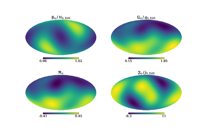
The general formalism presented in this section provides a consistent way of taking into account anisotropies in standard candle and standard siren data, without the need of imposing exact symmetries at the level of the metric tensor. If inhomogeneous and/or anisotropic features in the luminosity distance–redshift signal are sufficiently large in our Universe, these could significantly impact local measurements and our inference expansion and deceleration of space. The formalism can be extended to include model independent analysis of other observables, such as cosmological drift effects Heinesen:2021qnl .
VII.8.3 Local Void Scenario
A simple explanation of the tension could be that we live inside a bubble with a higher expansion rate—the so-called local void scenario.313131Here, we are not considering void models as alternative to dark energy, a scenario that has been strongly disfavored by kSZ constraints (Zhang:2010fa, ). For such a Hubble bubble model one expects that an adiabatic perturbation in density causes a perturbation in the expansion rate given by:
| (126) |
where is the present-day growth function for the concordance CDM model. It follows that, to have a % change in , one needs a Hubble bubble of contrast . As shown by Fig. 3, within the standard model, such contrasts are reached only at small scales. Therefore, one does not expect that a local structure could explain away the Hubble tension as is measured at larger scales (see again Fig. 3). As discussed in Sec. IV.6, estimates based on theoretical computations and numerical simulations suggest that cosmic variance on amounts at 0.51%.
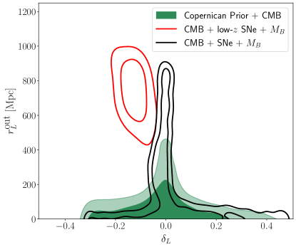
However, the previous reasoning assumes the standard model, in particular that the FLRW background can describe observations on cosmological scales. If one drops the FLRW assumption, there could be inhomogeneity around us of arbitrary depth and size.323232There could also be large-scale anisotropies, but these are much more constrained from observations (see, however, recent studies on large-scale dipole anisotropies (Siewert:2020krp, ; Secrest:2020has, )). Perturbations around us are expected to follow the power spectrum derived from the CMB (the one that was used for Fig. 3) only within the standard FLRW paradigm, which implies that the observer’s local Universe is statistically similar to the one at the last scattering surface. One can then study a model that features an arbitrary inhomogeneity around the observer and see how much observations can constrain such inhomogeneous model. Equivalently, one can reconstruct the metric from observations, checking if FLRW is recovered. To this end, the LTB metric with the cosmological constant (the LTB model) provides a convenient formalism to constrain deviations from FLRW (see Ref. Camarena:2021mjr and reference therein). Contrary to the Hubble bubble model, the LTB model features a smooth profile without discontinuities, allowing for a better comparison with observational data.
Ref. Camarena:2021mjr constrained the LTB model using the latest available data from CMB, BAO, type Ia supernovae, local , cosmic chronometers, Compton -distortion and kinetic Sunyaev–Zeldovich effect. Regarding the tension, it was found that, if one considers CMB, low-redshift supernovae from Pantheon () and the local calibration on the supernova magnitude from SH0ES Camarena:2021jlr , then a local underdensity of size –Mpc and contrast is indeed preferred by the data, see the red contours in Fig. 17. This structure is clearly non-Copernican and at strong odds with the standard model, which predicts the structures depicted by the green contours. However, if we include all the supernovae, one finds that the void scenario is ruled out and the FLRW limit is basically recovered (black contours in Fig. 17).
Specifically, when including only low- supernovae one finds . If instead, all supernovae are included, one finds : as the local structure is very much constrained by data, the value is close to the one inferred from CMB observations (see Ref. Camarena:2021-LLTB-H0 for more details). Concluding, assuming that CMB and supernova systematics are under control, an underdensity around the observer as modelled within the LTB model cannot solve the tension Wojtak:2013gda ; Odderskov:2014hqa ; Wu:2017fpr ; Kenworthy:2019qwq ; Cai:2020tpy ; Martin:2021wvb ; Castello:2021uad . See Sec. VII.8.2 for model-independent frameworks for analysing low-redshift cosmological data without imposing a particular form of the metric tensor.
VIII Challenges for CDM Beyond and
Coordinator: Leandros Perivolaropoulos.
Contributors: Özgür Akarsu, Yashar Akrami, Luis Anchordoqui, David Benisty, Anton Chudaykin, Craig Copi, Eleonora Di Valentino, Celia Escamilla-Rivera, Pablo Fosalba, Enrique Gaztanaga, Dragan Huterer, Andrew Jaffe, Chung-Chi Lee, Benjamin L’Huillier, Matteo Lucca, Roy Maartens, C.J.A.P. Martins, Suvodip Mukherjee, Pavel Naselsky, Eoin Ó Colgáin, Paolo Salucci, Arman Shafieloo, M.M. Sheikh-Jabbari, Foteini Skara, Glenn Starkman, Richard Watkins, John Webb.
In this section we discuss in a unified manner many existing signals in cosmological and astrophysical data that appear to be in some tension ( or larger) with the standard CDM model as defined by the Planck 2018 parameter values. In addition to the well known tensions discussed in previous sections ( tension and tension), there is a wide range of other less-discussed less-standard signals, at a statistical significance level lower than the tension, that may also constitute hints of new physics. The goal of this section is to collectively present the current status of these signals and their levels of significance, refer to recent resources where more details can be found for each signal and discuss possible generic theoretical approaches that can collectively explain the non-standard nature of these signals. It is worth stressing that some of the tensions are painting a coherent picture, whereas others are isolated and potentially even contradict tensions in and .
According to these ideas, we adopt the following strategic questions:
-
•
What are the current cosmological and astrophysical datasets that include such non-standard signals?
-
•
What is the statistical significance of each signal?
-
•
Is there a common theoretical framework that may explain these non-standard signals if they are of physical origin?
Along the same lines, a recent extensive broad review of non-standard signals may be found in Ref. Perivolaropoulos:2021jda , which has updated earlier works on the subject Perivolaropoulos:2008ud ; Perivolaropoulos:2011hp collecting and discussing signals in data that are at some statistical level in tension with the standard CDM model. In addition, interesting reviews focusing mainly on the Hubble tension may be found in Refs. DiValentino:2020zio ; Knox:2019rjx ; Jedamzik:2020zmd ; CANTATA:2021ktz ; DiValentino:2021izs ; Shah:2021onj , while other reviews focusing mainly on CMB anomalies may be found in Refs. Schwarz:2015cma ; Copi:2010na , and in Refs. Planck:2019evm ; Planck:2015igc ; Planck:2013lks .
In what follows, we provide a short example list of the non-standard cosmological signals in cosmological data. In many cases the signals are controversial and there is currently debate in the literature on the possible systematics origin of some of these signals. However, for completeness we refer to all signals we could identify in the literature referring also to references that dispute the physical origin of these signals.
VIII.1 The Anomaly in the CMB Angular Power Spectrum
The parameter was first introduced in Ref. Calabrese:2008rt . is an ”unphysical” parameter that actually rescales by hand the effects of the gravitational lensing on the CMB angular power spectra, and can be computed by the smoothing of the peaks in the damping tail. For example, indicates no lensing effect, whilst for one recovers the value expected in GR. It is quite interesting to note that for Planck CMB power spectra one finds a preference for at more than 95% CL for both Plik and CamSpec likelihoods, with a large improvement of the . Moreover, the inclusion of BAO data shows an evidence for at more than CL for Plik likelihood and about 99% for the CamSpec likelihood.
The evidence for is not easily describable in the existing theoretical frameworks and this requires some new challenges in theory, for example, we need either a closed Universe model and surely challenge several observational datasets and the simplest inflationary models, see Ref. DiValentino:2019qzk ; Handley:2019tkm ; DiValentino:2020hov and subsection VIII.2, or we need more exotic cosmological theories that would lead to modifications of the GR Planck:2015bue ; DiValentino:2015bja ; Planck:2018vyg , a running of the running of the spectral index Cabass:2016ldu , or compensated baryon isocurvature perturbations Munoz:2015fdv ; Valiviita:2017fbx , or a Ginzburg-Landau Theory of DE Banihashemi:2022vfv . Moreover, this lensing anomaly is not observed in the Planck trispectrum data (i.e. CMB lensing) which offer a complementary and independent measurement of the parameters. If the anomaly does not call for a new physics, then this anomaly may connect to a mild but undetected systematic error in all the releases of the Planck data Planck:2013pxb ; DiValentino:2013mt ; Planck:2015fie ; Planck:2018vyg that one cannot rule out from the current picture. If is related to systematics, then we need to understand how this systematic could affect the constraints on the Hubble constant or S8 parameter, and hence on the different tensions explored in this work.
A recently developed method to directly constrain the CMB gravitational lensing potential from the CMB data is based on a principal component decomposition of the lensing power spectrum Motloch:2018pjy . This approach extends the usual analysis by introducing arbitrary shape variations around a fixed fiducial lensing power spectrum. Marginalizing over effective parameters leads to interesting implications in various extensions of the CDM model. In the CDM+ scenario marginalizing lensing substantially broadens the constraints, at 68% CL Motloch:2019gux . The lensing-like anomaly also strengthens the constraints on neutrino masses. In fact, ignoring Planck lensing reconstruction ie allowing for an arbitrary gravitational lensing potential one finds eV at Motloch:2019gux which is three times weaker than the Planck constraint. On the other hand when including BAO, supernova constraints, and Planck lensing reconstruction, the neutrino mass constraint degrades only by over the Planck constraint after marginalizing over lensing information .
The latest ACT measurements find no deviation from the standard lensing effect predicted in the CDM model, ACT:2020gnv . Recent measurements of TE and EE power spectra collected by SPT-3G are also consistent with the standard model prediction, SPT-3G:2021eoc . Finally, combining Planck TT () and SPTPol polarization and gravitational lensing measurements arrives at Chudaykin:2020acu . These results indicate that the lensing anomaly persists only in the Planck data at small scales and is absent for other CMB experiments. Forecasts for future CMB data have been performed in Ref. Renzi:2017cbg .
VIII.2 Hints for a Closed Universe from Planck Data
The enhanced lensing amplitude ( anomaly Calabrese:2008rt ; Planck:2018vyg ) in the CMB power spectrum indicated by the different Planck data releases is a significant challenge for the standard CDM model. A physical explanation for this enhancement could be provided in the context of a closed Universe which due to this anomaly, is preferred over a flat Universe at a level of DiValentino:2019qzk ; Planck:2018vyg ; Handley:2019tkm .333333There is a related preference of the Planck dataset at more than for Modified Gravity Planck:2018vyg ; DiValentino:2015bja ; Planck:2015bue ; Capozziello:2002rd . This disagreement with the predictions for a flat Universe of the standard model is due to the strong degeneracy between the parameter Calabrese:2008rt ; Planck:2018vyg , and the spatial curvature parameter as indicated in Fig. 18. A closed Universe could also reduce the well-know tension between the low and high multipoles of the angular CMB power spectrum Addison:2015wyg ; Planck:2016tof ; DiValentino:2019qzk . The oscillating features of the CMB power spectrum indicating spatial curvature could be due to unresolved systematics in the Planck 2018 data, or can be simply due to statistical fluctuations.
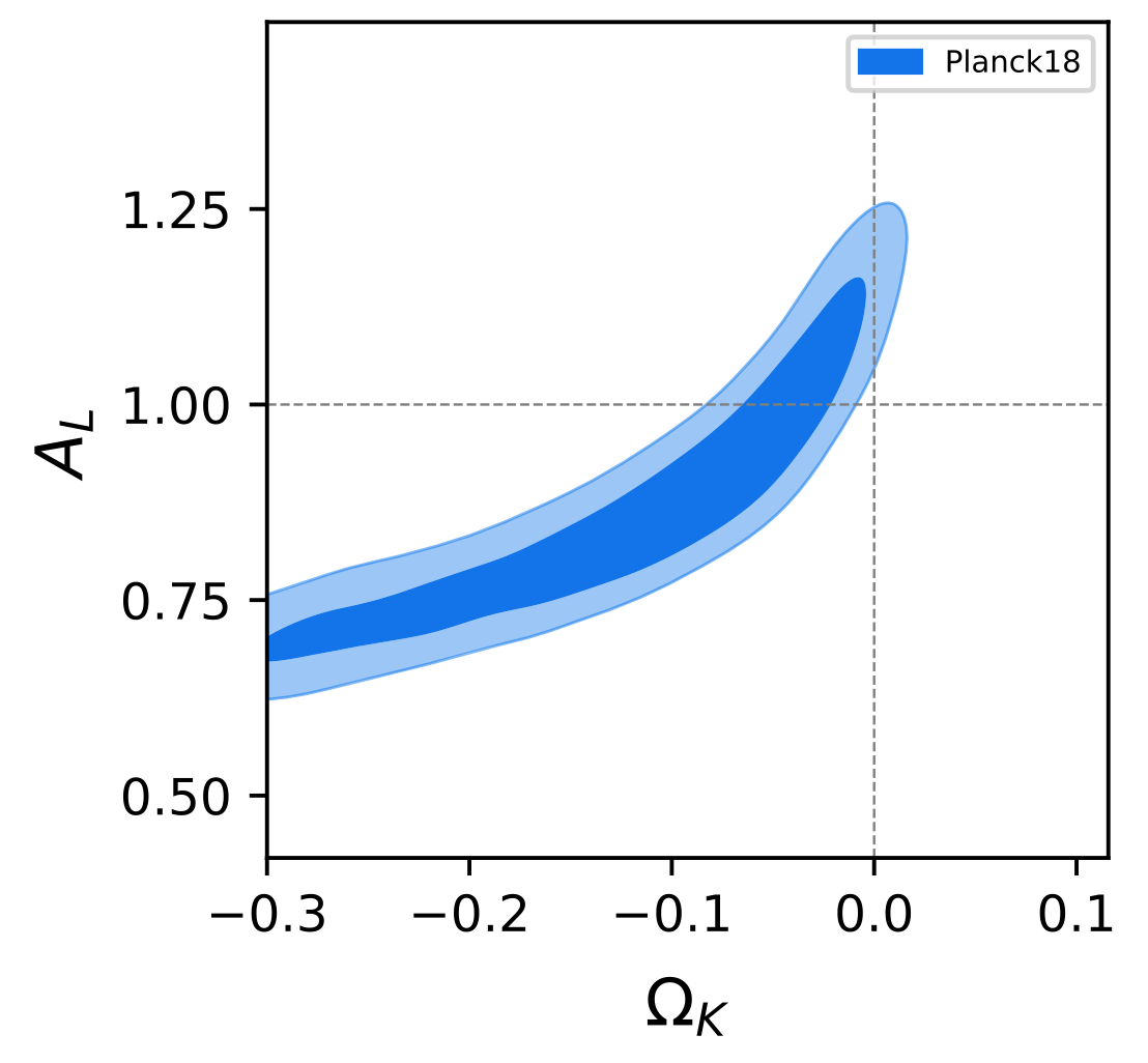
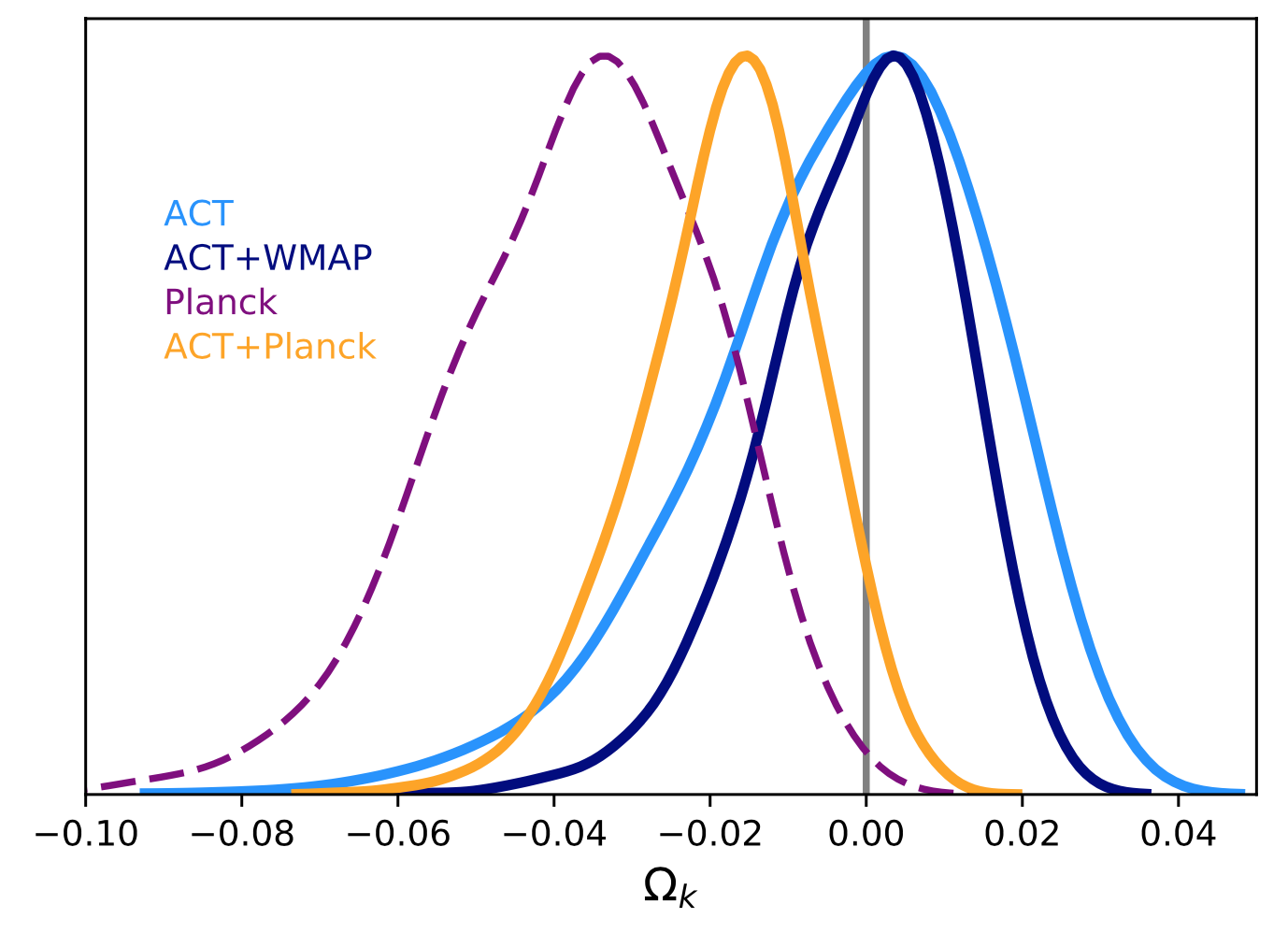
In fact, while Planck 2018 Planck:2018vyg finds ,343434All the bounds are reported at 68% confidence level in the text. i.e. at about () using the baseline Plik likelihood Planck:2019nip , the evidence is reduced when considering the alternative CamSpec Efstathiou:2019mdh likelihood (see discussion in Efstathiou:2020wem ), albeit with the marginalized constraint still above the CL ().
If anomaly demands for more lensing, and this is connected to an increase in the cold dark matter density, then it could be explained by a closed Universe. However, in this case, from Planck could be very small, something like Planck:2018vyg ; DiValentino:2019qzk ; Handley:2019tkm , exacerbating the Hubble tension as well as the tension.
Other combinations of data considered in the literature appear to favor (or not favor) a closed Universe at varying levels of statistical significance. In particular:
-
•
The recent results from the ground-based experiment ACT, in combination with data from the WMAP experiment, are fully compatible with a flat Universe with .
-
•
The same ACT data when combined with a portion of the Planck dataset lead to slight preference for a closed Universe since in this case ACT:2020gnv , see Fig. 18.
-
•
A closed Universe is preferred by a combination of non-CMB data obtained by Baryon Acoustic Oscillation (BAO) measurements Beutler:2011hx ; Ross:2014qpa ; Alam:2016hwk ; Benisty:2020otr , SNIa distances from the recent Pantheon catalog Pan-STARRS1:2017jku , and a prior on the baryon density derived from measurements of primordial deuterium Cooke:2017cwo assuming Big Bang Nucleosynthesis (BBN). In the context of this combination, a much larger DiValentino:2019qzk is obtained in agreement with the SH0ES value Riess:2021jrx ; Riess:2019cxk of .
-
•
A flat Universe is preferred by the combination Planck + BAO, or + CMB lensing Planck:2018lbu or + Pantheon data. However these dataset combinations are in disagreement at more than when the curvature is allowed to vary DiValentino:2019qzk ; Handley:2019tkm ; Vagnozzi:2020rcz .
-
•
A phantom closed Universe is preferred by Planck combined with the luminosity distance probes, such as Pantheon or SH0ES, when the dark energy equation of state is let free to vary, along the curvature, at more than 99% CL DiValentino:2020hov .
-
•
A flat Universe is also in agreement with the analysis made by Liu:2020pfa using the sample from the cosmic chronometers (CC) and the luminosity distance from the 1598 quasars () or the Pantheon sample (), in agreement with the previous analysis of Cai:2015pia (in these analyses however, the error bars are too large to discriminate among the models).
-
•
In Nunes:2020uex a combination of BAO+BBN+H0LiCOW provides with in agreement with R19, while BAO+BBN+CC gives a positive .
-
•
The curvature can also be measured model-independently via the parameter Clarkson:2007pz ; LHuillier:2016mtc ; Marra:2017pst ; Shafieloo:2018gin
(127) which is constant and equal to the curvature parameter in an FLRW Universe. Departures from constancy could point towards departure from FLRW or the presence of systematics in the data. Current data (Supernovae from Pantheon and BAO from BOSS) are consistent with a flat FLRW LHuillier:2016mtc ; Shafieloo:2018gin .
-
•
Another approach is to use three distances between a source, lens, and the observer to estimate the curvature independently from cosmological assumptions Rasanen:2014mca ; Denissenya:2018zcv . This does not involve any derivative and is consistent with a flat Universe in the context of large uncertainties.
Overall, the spatial curvature remains insensitive to local measurements from the Cepheid distance ladder Zuckerman:2021kgm . However, in general, letting the curvature free to vary implies an increase of both the and the tensions DiValentino:2019qzk . Therefore, the constant-curvature degree of freedom of the standard model is not sufficient to explain the tensions and anomalies seen in the data. However, within full GR, in the context of the scalar averaging scheme, the average scalar curvature can provide considerably stronger evolutionary impact Heinesen:2020sre .
Detecting a curvature different from zero could be due to a local inhomogeneity biasing our bounds Bull:2013fga , and in this case CMB spectral distortions such as the KSZ effect and Compton-y distortions, present a viable method to constrain the curvature at a level potentially detectable by a next-generation experiment. If a curvature different from zero is the evidence for a truly superhorizon departure from flatness, this will have profound implication for a broad class of inflationary scenarios. While open Universes are easier to obtain in inflationary models Gott82 ; Linde:1998gs ; Bucher:1994gb ; Kamionkowski:1994sv ; Kamionkowski:1993cv , with a fine-tuning at the level of about one percent one can obtain also a semi-realistic model of a closed inflationary Universe Linde:2003hc ; Lasenby:2003ur . In Ref. Leonard:2016evk it has been shown that forthcoming surveys, even combined together, are likely to place constraints on the spatial curvature of at 95% CL at best, but enough for solving the current anomaly in the Planck data. Experiments like Euclid and SKAO, instead, may further produce tighter measurements of by helping to break parameter degeneracies DiDio:2016ykq ; Vardanyan:2009ft .
VIII.3 Large-Angular-Scale Anomalies in the CMB Temperature and Polarization
Several features unexpected in CDM cosmology have been noted in CMB temperature fluctuations at the largest angular scales. Most of these anomalies share several common features:
-
•
they refer to the largest observable angular scales – whether directly as large-angle two-point functions (lack of large-angle correlations, quadrupole-octopole anomalies), or as large-angle modulations of smaller-angular-scale fluctuations (hemispherical asymmetries, point parity anomaly);
-
•
they are not captured in a standard experimental CDM likelihood function because they are not deviations of individual from the values predicted by CDM with appropriate parameters; they are therefore characterized by statistics that were proposed post-facto to capture a pattern noticed in the data;
-
•
WMAP and Planck are in remarkable agreement about them being real features on the sky.
An additional anomaly, that is on somewhat smaller scales (), but shares the other features, is the so-called ”cold spot.”
We now describe the most compelling of these anomalies:
-
1.
the lack of large-angle CMB temperature correlations;
-
2.
hemispherical power asymmetry;
-
3.
octopole planarity and alignment with the quadrupole;
-
4.
the point-parity anomaly;
-
5.
variation in cosmological parameters over the sky;
-
6.
the cold spot.
In contrast to the Hubble constant tension (), these anomalies are individually statistically less significant ( to ). However, within CDM, they appear to be statistically independent, although this has been rigorously demonstrated only for the first and last of the above list. Jointly, they are highly significant. An understanding of their nature can point to new physics in the primary perturbations formation process or shed light on unaccounted systematic effects in both astronomical and CMB data Planck:2015igc ; Planck:2019evm .
We make clear below why these anomalies are difficult to explain in the context of CDM. We explore the CDM predictions for analogous statistics (if any) for polarization, and contrast those predictions with what might be expected from explanations of the anomalies based on new physics. Finally, we discuss how future experiments could be valuable and why they should make the testing of these predictions a key element of their scientific programs.
VIII.3.1 The Lack of Large-Angle CMB Temperature Correlations
Suppressed correlations at the largest observable angular scales had been noticed in the COBE data Bennett4766 . Specifically, the two-point angular correlation function
| (128) |
(where the average is over all pairs of pixels with ) was found to be very close to zero on scales above Hinshaw:1996ut . The near-vanishing of the large-angle correlation function was clear in the early WMAP data WMAP:2003elm , and was later confirmed in the 3-yr Copi:2006tu and the 5-yr WMAP data in Copi:2008hw , as well as in the Planck data Copi:2013cya .
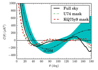
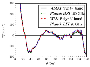
Fig. 19, adopted from Ref. Copi:2013cya , illustrates the degree to which the correlations are suppressed on the cut sky (part of the sky not contaminated by Galactic emission) for both WMAP and Planck. The most striking feature of the cut-sky is that it is very nearly zero above about , except for some anti-correlation near . This is true for all reasonable Galaxy masks, for all WMAP and Planck CMB-dominated wavebands, in all data releases. It is also true for calculated from the pseudo- using .
In order to be more quantitative about these observations, the WMAP team WMAP:2003elm introduced a statistic that quantifies the deviation of from zero,
| (129) |
Spergel et al. WMAP:2003elm found that only of the realizations in their Markov chain of CDM model CMB skies had lower values of than the observed one-year WMAP cut sky. Extending this to later releases of WMAP data, as well as Planck, the p-value becomes ballpark , depending on the map and mask used Copi:2013cya ; see again Fig. 19. There have been some suggestions that certain three-point and four-point functions are also anomalous Planck:2013lks ; Planck:2015igc ; Eriksen:2004iu ; we discuss that below in the context of hemispherical asymmetry, where this anomaly is more evident.
While computed in pixel space over the masked sky agrees with the harmonic space calculation that uses the pseudo- estimator, it somewhat disagrees with the obtained from a variety of foreground-corrected reconstructed full-sky maps. The latter however agree with the calculated using the maximum-likelihood estimator (MLE) that are typically reported. These have that are low only at the level Copi:2011pe . However, problematically, the full-sky map is dominated by pairs of points at least one of which is in the masked region, suggesting that the full-sky is potentially contaminated by artefacts coming from the galactic plane. Nevertheless, it is the angular correlation function observed on unmasked, ”clean” portions of the sky that is statistically low at the level of – (depending on the choice of the map and the sky cut).
In Ref. Efstathiou:2009di it is argued that cannot be used to exclude the CDM model. The relevant low- have large cosmic variance as a fraction of their expected values, so inferred can differ markedly from the expected values. This results in very large sampling covariance error predictions for in CDM. Moreover could be small because the CDM predictions have more power on the low than the actual CMB measurements. The significance of the discrepancy then depends on the model assumptions Gaztanaga:2003ub ; Camacho-Quevedo:2021bvt . Nevertheless, using model-independent errors, based only on direct measured sampling variations, Ref. Camacho-Quevedo:2021bvt finds strong evidence for a homogeneity scale and lack of correlations on scales larger than degrees on the CMB sky.
It is widely underappreciated, however, that the smallness of is not primarily due to the smallness of any individual nor set of s, and so is not accurately described as a ”lack of large-angle power”. Rather, it is due to cancellations among the contributions of the low- to up to at least — is almost optimal Copi:2008hw to cancel the contributions of . In other words, . The fractionally large variance in the low- actually makes such correlations less likely to emerge accidentally. Such correlations between do not feature (at least at leading order) in vanilla CDM likelihoods, because CDM says that there are no such correlations. Thus parameter fitting within CDM, comparisons of CDM with other statistically isotropic models, and even goodness-of-fit tests of CDM will not be sensitive to these correlations—they are either statistical flukes, or evidence of a violation of a fundamental assumption of vanilla CDM.
Thus the anomaly as realized on the observed sky is evidence for the violation of statistical isotropy, which we might expect to result also in more general correlations between as we discuss below. Explanations of this anomaly are relevant only if they accomplish it through such cancellation and not by reducing low- . This cannot be accomplished by, for example, changing the primordial power spectrum . Non-trivial topology has been shown to be able to produce low with appropriate Bernui:2018wef , albeit with a fundamental domain that is ruled out by the absence of pairs of matched circles in CMB maps Vaudrevange:2012da .
In Ref. Aurich:2021ofm it is argued that the lack of power on large scales may be simply due to the fact that our Universe is of a finite topology. Samples of 100,000 CMB maps with cubic 3-torus topology are shown to be consistent with the large-angle CMB temperature correlations, when the Dirichlet domain side length of our Universe is around three times the Hubble length. Meanwhile, the angular scale corresponds to the causal horizon of a Universe Camacho-Quevedo:2021bvt , which is in agreement with the super-horizon anomalies found in the fit to the small scale CMB acoustic peaks, see below in Sec. VIII.3.5.
Predictions.
Given the concern that this anomaly (and others) are based on a posteriori statistics, with unknown look-elsewhere effects, to be more fully convinced that they are due to new physics, rather than a statistical fluke, requires testable predictions. The first type of predictions come from CDM conditioned on one or more anomaly (or more generally on the measured temperature maps); these can be used to test the ”fluke hypothesis” that the anomalies are not signs of new physics. The second type of predictions would best come from a model of new-physics. However, even absent that one can in some cases argue generically that a physical explanation would likely have certain consequences.
Prediction for : An important point that is widely overlooked is that as discussed above is actually the monopole-and-dipole subtracted angular correlation function, which we write . A physical explanation of seems likely to predict that is small, not just . This requires that the cosmological (i.e., non-Doppler) contribution to Copi:2013cya . This happens by chance less than of the time in CDM with standard cosmological parameters, and so if a low were observed it would be compelling evidence of a physical origin for low . This suggests that measuring the CMB Doppler dipole well enough to separate out the intrinsic is worthwhile. Similar statements could perhaps be made about the cosmological monopole , the fluctuation in in our current Hubble patch about the mean calculated over an infinite, or at least much larger volume, but that is presumably not measurable.
Predictions for Polarization: CDM realizations of temperature and -mode and -mode polarization are usually generated together, with , and correlated Gaussian random variables characterized by , , and , while is a Gaussian random variable characterized by . However, given measurements of , one can produce constrained realizations of Yoho:2013tta ; realizations of are unchanged since is uncorrelated with . One can then calculate and , for the Q and U mode polarizations, and assemble predictions for , , , , and , as well as associated statistics, Because correlations are weak in CDM (), the suppression of does not lead to the suppression of QQ and UU angular correlation functions Yoho:2015bla , with, for example, and for , essentially unchanged from unconstrained CDM. A low measured value for either would be a statistically independent anomaly for CDM. Meanwhile, it would be expected that a physical model would predict suppression of these correlation functions.
There is some subtlety regarding angular correlation functions for polarization Yoho:2015bla . Whereas, once certain conventions have been established, and are fields measured on the sky, the separation into and is performed in harmonic space, and the reassembly into and is ambiguous. The local-E and local-B fields Yoho:2015bla , and , are heavily weighted toward high- contributions, and in particular the usual to correspondence fails for for or . This makes and independently interesting Yoho:2015bla , both as null tests for CDM and as tests of physical explanations for the low . It is also possible to put other two-point angular correlation functions to good use, such as between temperature and lensing potential, or temperature and 21-cm fluctuations. In such cases, the optimum range of over which to integrate should be determined a priori Yoho:2013tta . Future full-sky polarization observation programs could readily measure all interesting polarization statistics and test the CDM predictions Yoho:2015bla .
VIII.3.2 Hemispherical Power Asymmetry
Here, we focus on a number of large-scale anomalies, which in spite of having been detected with different methods and statistics, all show some level of asymmetry in power (or related properties) between hemispheres on the CMB sky; this is why we collectively call them ”hemispherical power asymmetry.” We do not intend to provide an historical overview of these anomalies or an exhaustive review of the literature on detection, analysis and interpretation of the anomalies. Our aim in this subsection is rather to highlight the most statistically significant hints of the power asymmetry and their common features, with the objective of emphasising their potential importance for both theoretical cosmology and future CMB and large-scale-structure observations.
The bulk of this section discusses tests that involve the so-called dipolar power asymmetry or ”dipole modulation,” either directly or via measures of directionality, even though there are reasons to believe that such a dipolar description of the asymmetry oversimplifies the actual anomaly. One main reason is that most of the analyses imply that only the hemispheres which include all or most of the northern ecliptic hemisphere are anomalous and the southern ones seem to be consistent with an isotropic CDM CMB sky. Nevertheless, various forms of dipole modulation have been noted since the early WMAP releases Eriksen:2003db and later confirmed by Planck Planck:2013lks ; Planck:2015igc ; Planck:2019evm . All the dipole-modulation tests we discuss here can be divided into two categories, amplitude-based and direction-based, and share in common the fitting of a dipole, which is done either by fitting for a dipole explicitly in a map of power on the sky, by employing Bayesian techniques in pixel space for a specific model, or by measuring the coupling of to modes in the CMB covariance matrix. Given the differences in the approaches, it is important to keep in mind that the results cannot usually be directly compared, even though all probe some aspect of dipolar asymmetry.
Low Northern Variance.
A low value for the variance of the CMB temperature fluctuations was originally observed in the WMAP data by Refs. Monteserin:2007fv ; Cruz:2010ud ; Gruppuso:2013xba . This low variance was then confirmed by the Planck collaboration Planck:2013lks ; Planck:2015igc ; Planck:2019evm , with a -value of - for the low-resolution temperature maps (), depending on whether the impact of a possible look-elsewhere effect is considered. Planck 2013 Planck:2013lks showed, using both full-resolution () and low-resolution () maps that the low variance was localised in the northern ecliptic hemisphere, with a -value of , while the -value for the southern hemisphere was . Similar levels of significance were also found for the Galactic northern and southern hemispheres when the full-resolution maps were used. No updates on these significance levels have been provided by Planck 2015 Planck:2015igc and 2018 Planck:2019evm . It is important to note that the map-based variance is dominated by contributions from large angular scales, whilst the cosmological parameter fits are relatively insensitive to these low-order -modes and are instead largely dominated by scales corresponding to . Therefore, the variance of the temperature CMB sky appears to be anomalous as there is a dearth of large-angular-scale power compared to the predictions of the CDM model with parameters estimated using the same CMB sky. Finally, it is important to note that although the anomaly discussed here is about the variance of the CMB fluctuations, it can be seen as an indirect indication of power asymmetry, as variance is nothing but a weighted sum of the angular power spectrum of the fluctuations over all multipoles.
Hemispherical Asymmetry.
Refs. Eriksen:2003db ; Hansen:2004vq discovered that the angular power spectrum of the first year WMAP data calculated for a hemisphere centred at the Galactic coordinates was larger than when calculated for the opposite hemisphere over the multipole range . Ref. Park:2003qd also presented evidence for the existence of such hemispherical asymmetry by applying a Minkowski functional to the WMAP data. The preferred direction of Ref. Eriksen:2003db lies close to the ecliptic plane, and they also demonstrated that the large-angular real-space -point correlation functions (for ) were different when computed on ecliptic hemispheres. Many studies then focused on hemispheres in the ecliptic coordinate system, with Ref. Schwarz:2004gk particularly emphasizing the connection. Finally, Refs. Eriksen:2004df ; Eriksen:2004iu ; Rath:2007ti also detected the hemispherical asymmetry with other measures of non-Gaussianity.
In 2013, the Planck collaboration Planck:2013lks studied the asymmetry by computing four -point correlation functions (2-point function, pseudo-collapsed 3-point function, equilateral 3-point function and rhombic 4-point function) on the northern and southern ecliptic hemispheres for the Planck 2013 temperature maps. The results were in agreement with the findings of Ref. Eriksen:2003db . It was shown, particularly, that the northern ecliptic hemisphere correlation functions were relatively featureless, and in particular, both the 3- and 4-point functions were very close to zero. The northern hemisphere -values for the statistic were found to be for all the four correlation functions and for the 3- and 4-point functions, with the significance level exceeding for the pseudo-collapsed 3-point function. This was all consistent with the anomalous lack of power towards the northern ecliptic pole seen by the simpler one-point statistic, i.e. the low northern variance anomaly discussed earlier. Similar analyses were done in reference frames set by Galactic coordinates and the CMB Doppler boost direction (see e.g. Quartin:2014yaa ), as well as the angular-clustering and dipole-modulation directions that we will discuss below. Although the largest asymmetry was seen for the ecliptic hemispheres, a substantial asymmetry was present also for Galactic coordinate hemispheres.
The Planck 2015 analysis Planck:2015igc confirmed all of these high levels of significance, and additionally found that a substantial asymmetry was present also for the dipole-modulation direction. Surprisingly though, the latest Planck 2018 analysis Planck:2019evm no longer observed the high significance level for the pseudo-collapsed 3-point function of the temperature map in the northern ecliptic hemisphere. The Planck collaboration states Planck:2019evm that this discrepancy between the first two and the final releases of the data may be due to the different masks used in the analyses or a consequence of ”the improved treatment of poorly determined modes in the estimated correlation matrix used for the computation of the statistic.” Even if these are the reasons behind the discrepancy, the fact that the anomaly has been observed persistently and consistently in both the WMAP data and the first two releases of the Planck data (with different systematics) strongly suggests that the changes in the mask or the improvement in the analysis might have removed important information in the data that would contribute significantly to this anomaly, and the low significance seen in the Planck 2018 data should therefore be considered with caution. Planck 2018 found, however, that in the dipole-modulation reference frame the 3-point temperature correlation functions in the negative (northern) hemisphere were somewhat significant, reaching a level of for the pseudo-collapsed case.
Angular Clustering of the Power Distribution.
In a search for dipolar power asymmetry, Ref. Hansen:2008ym analysed the 5-year WMAP data by computing the CMB power spectrum on a number of discs on the sky and binning them into independent blocks of 100 multipoles from to . Each block was then used to look for a dipolar asymmetry in the power distribution. The six ranges considered showed evidence of a consistent dipole direction, and not a single realization in a set of 10,000 simulations showed a similarly strong asymmetry.
A similar analysis was then performed by the Planck collaboration in 2013 Planck:2013lks , where a simpler approach developed by Ref. Axelsson:2013mva and applied to the 9-year WMAP data was used. Planck 2013 estimated the power spectrum amplitude on 12 non-overlapping patches of the sky in -bins of 16 multipoles each, and fitted a dipole to the spatial distribution of the amplitudes for each -bin. The alignment of the dipole directions between the different multipole blocks was then used to construct a measure of the power spectrum asymmetry. They compared the clustering of the dipole directions evaluated for the different scales to that observed in simulated maps. None of the 500 available simulations showed degrees of clustering higher than the one observed in the data for two choices of and . However, after deboosting the data (i.e. correcting for the Doppler modulation effect), the significance went down for , and therefore, a significant power asymmetry was claimed only up to . The deboosted case, however, resulted in the mean dipole direction of , which was intriguingly close to the direction found for the dipole modulation, as we will discuss below. Even though a power asymmetry was detected using the angular clustering of the preferred directions for different bins, the ratio of the power spectra in the two opposite hemispheres defined by the asymmetry axis for was not statistically anomalous. The interpretation for this was that the power asymmetry detected through the clustering technique might be different from the one found by other methods with statistics based on the amplitude of the asymmetry, usually quantified by a dipole (as done, e.g., in the cases of dipole modulation and local-variance asymmetry discussed below).
In an updated and extended analysis, Planck 2015 Planck:2015igc considered bin sizes between and for the multipole range of . In contrast to the Planck 2013 results where the -values started to increase systematically for , here they remained low for . Depending on the bin size and component separation method, -values were as low as . These all suggest that, beyond a dipole modulation of power on large angular scales, some form of directional asymmetry continues to small scales. There are also indications that the directions of dipolar asymmetry are correlated between large and small angular scales.
Dipole Modulation (Pixel-Based Likelihood).
Even though no compelling theoretical explanation exists for the nature of the hemispherical power asymmetry, a phenomenological multiplicative dipole modulation model, suggested by Ref. Gordon:2005ai , has been widely used to study the asymmetry through a model-dependent, Bayesian approach. Here, the asymmetry is modeled in terms of a dipole modulation of the form
| (130) |
where and are the isotropic and modulated CMB temperature fluctuations along a direction on the sky, respectively, and is the amplitude of the dipole modulation and is the preferred direction.
It is important to note that since various other analyses of the CMB sky seemed to imply that the southern hemisphere was relatively consistent with an isotropic CDM sky and it was the northern hemisphere that showed an anomalous deficit of power, the dipole modulation may not be a well justified way of modeling the asymmetry; it has been used mainly because of its simplicity. Refs. Eriksen:2007pc ; Hoftuft:2009rq studied the dipole modulation model using the 3- and 5-year WMAP data, respectively, and the Planck collaboration then performed a similar direct pixel-space likelihood analysis of the model in their 2013 Planck:2013lks and 2015 Planck:2015igc investigations of the hemispherical power asymmetry by only considering large angular scales. Planck used temperature maps, smoothed to angular resolutions ranging from to FWHM. Planck 2015 particularly focused on a smoothing scale of FWHM as a representative example and the highest angular resolution accessible for an map. The results of the analysis were all consistent with those derived from the 5-year WMAP ILC map in Ref. Eriksen:2007pc . The significance levels for the amplitude of the dipole compared to the ones from the CDM simulations varied with smoothing scale and the scale showed the highest significance (). It is important to note that the model of Ref. Gordon:2005ai assumes that the modulation amplitude is equally strong on all scales, but it has been shown Quartin:2014yaa ; Notari:2013iva that the data are not consistent with a simple constant-amplitude dipole modulation of the power. The preferred direction derived from the low- dipole modulation analysis, e.g. for the Commander component separation technique, is, however, remarkably consistent with the high- direction derived from the clustering of directions for . Both Planck 2013 and 2015 found almost exactly the same preferred directions.
Dipole Modulation (QML Analysis).
In a harmonic-space analysis, Planck 2015 Planck:2015igc used the quadratic maximum likelihood (QML) estimator introduced by Ref. Moss:2010qa to assess the level of dipole modulation for the full-resolution () CMB temperature maps. This technique exploits the fact that dipole modulation is equivalent to coupling of to modes in the CMB covariance matrix to leading order. Planck computed -values of the fitted modulation amplitude as a function of , and the -values showed several peaks, at , and . The latter peak, while not previously emphasized, was also present in the WMAP results Bennett:2010jb . The dip at , with a -value of (), corresponds to the low- dipole modulation, which has been the focus of most attention in the literature.
Planck 2018 Planck:2019evm repeated the analysis and studied two ranges of and . The preferred direction for the former range was found to be , while it was for the Planck 2015 analysis Planck:2015igc , both of which are consistent with the directions found through the pixel-based likelihood analysis of dipole modulation. One should note that this QML analysis was a purely phenomenological one performed in multipole space, with no attempt to connect to any real-space modulation. Even though the preferred directions are close to that of a pixel-space likelihood analysis of the dipolar modulation model, the two methods do not necessarily probe the same thing.
Meanwhile, WMAP also observed a dip in the first Doppler peak (), an excess at , and a dip at that were present in the ecliptic polar data but not the ecliptic planar data, see Fig. 7 of the first arXiv version of their Year 1 paper on the angular power spectrum WMAP:2003zzr . That first peak dip was shown in Ref. Yoho:2010pb to be localized to the region of the north ecliptic pole, and to persist beyond WMAP1 into later WMAP data releases. This is consistent with the dip’s presence in ARCHEOPS data, taken in the northern hemisphere, but in no other pre-WMAP ground-based data.
Dipole Modulation (Rayleigh Statistic).
The results of the analysis of the angular clustering of the power distribution performed by the Planck collaboration and discussed above suggest that, beyond a dipole modulation of power on large angular scales, some form of directional asymmetry continues to small scales. There are also indications from the same analysis that the directions of dipolar asymmetry are correlated between large and small angular scales. Planck 2015 Planck:2015igc then performed a Rayleigh-statistic-based analysis as a generic test for directionality with minimal assumptions about the nature of the asymmetry. The method, however, takes into account other information pertaining to modulation, including its amplitude, in addition to the direction. An asymmetry was found on scales larger than , and the minimum -value was , to be compared to the -value of obtained for the dipole modulation amplitude at . The preferred direction for was found to be , which is approximately away from the dipole modulation direction determined by the QML analysis for the multipole range of .
Generalised Dipole Modulation (Bipolar Spherical Harmonics).
The Planck collaboration studied, in both their 2013 Planck:2013lks and 2015 Planck:2015igc analyses, a generalisation of the dipole modulation using the Bipolar Spherical Harmonics (BipoSH) formalism of Refs. Hajian:2003qq ; Hajian:2006ud . Here, the CMB angular power spectrum corresponds to the BipoSH coefficients and a dipole modulation corresponds to the bipolar multipole . The BipoSH formalism provides a unified way to systematically detect and study properties of different types of statistical anisotropy, which may go beyond the dipole modulation. A BipoSH-based simulation tool is available to model Gaussian realizations of CMB temperature and polarization maps with induced isotropy violation Mukherjee:2013kga . Planck 2013 applied the BipoSH formalism to temperature maps and detected a dipole modulation signal with to significance, depending on the component separation method. The amplitude and direction of the dipole modulation matched those obtained via the likelihood analysis of dipole modulation. Both Planck 2013 and 2015 also used higher-resolution maps, but the dipole modulation was recovered at over significance only for the lowest multipole bin they considered, i.e. . For the full-resolution maps, Planck 2015 found a preferred direction of , in very good agreement with the direction inferred from the likelihood analysis of dipole modulation. No significant power was detected at the higher BipoSH multipoles of the modulation field, . Assuming a scale-dependent dipole modulation, Ref. Shaikh:2019dvb has measured this scale dependence using the BipoSH formalism.
Variance Asymmetry.
In an attempt to study the observed CMB power asymmetry in a model-independent way, Ref. Akrami:2014eta invented a pixel-space local-variance estimator of the CMB fluctuations using a set of discs of various sizes uniformly distributed on the sky. The technique was first applied to the WMAP 9-year and Planck 2013 temperature data in Ref. Akrami:2014eta and later used in the analyses of Planck 2015 Planck:2015igc and 2018 Planck:2019evm for both temperature and polarisation. Since the technique looks for deviations from statistical isotropy in terms of the variance of CMB fluctuations by fitting a dipole to a given local-variance map, it can be considered as an alternative way of detecting the hemispherical power asymmetry which had already been detected through the dipole modulation analysis and the angular clustering of dipole directions. This is because variance is effectively a weighted sum of the power spectrum over all scales (or multipoles).
The original analysis of Ref. Akrami:2014eta found that none of the available CMB temperature simulations had a larger variance asymmetry than that estimated from the data. This suggested presence of a power asymmetry at a statistical significance of at least , with a preferred direction of , in good agreement with other studies of the hemispherical power asymmetry. The local-variance estimator was then applied to the full-resolution Planck 2015 temperature maps Planck:2015igc , and significantly low -values were found, although the significance levels and preferred directions showed slight differences for different disc radii. The highest statistical significance was found for discs with -values less than . In an analysis with enhanced sky coverage, where a mask smaller than the Planck’s common mask was used, a number of anomalies were restudied through an Commander temperature map which included about of the sky. While in general the significance levels and preferred directions for the hemispherical power asymmetry inferred from different techniques did not change much with this reduced mask, the local-variance asymmetry method showed higher significance for larger disc radii. The variance asymmetry technique was finally applied to the Planck 2018 temperature data Planck:2019evm and -values smaller than were found for disc radii up to when the full-resolution maps were analysed. The preferred direction was found to be for this resolution and for discs, and changed slightly for lower-resolution maps; the direction was found to be for ; see Fig. 20 (left panel).
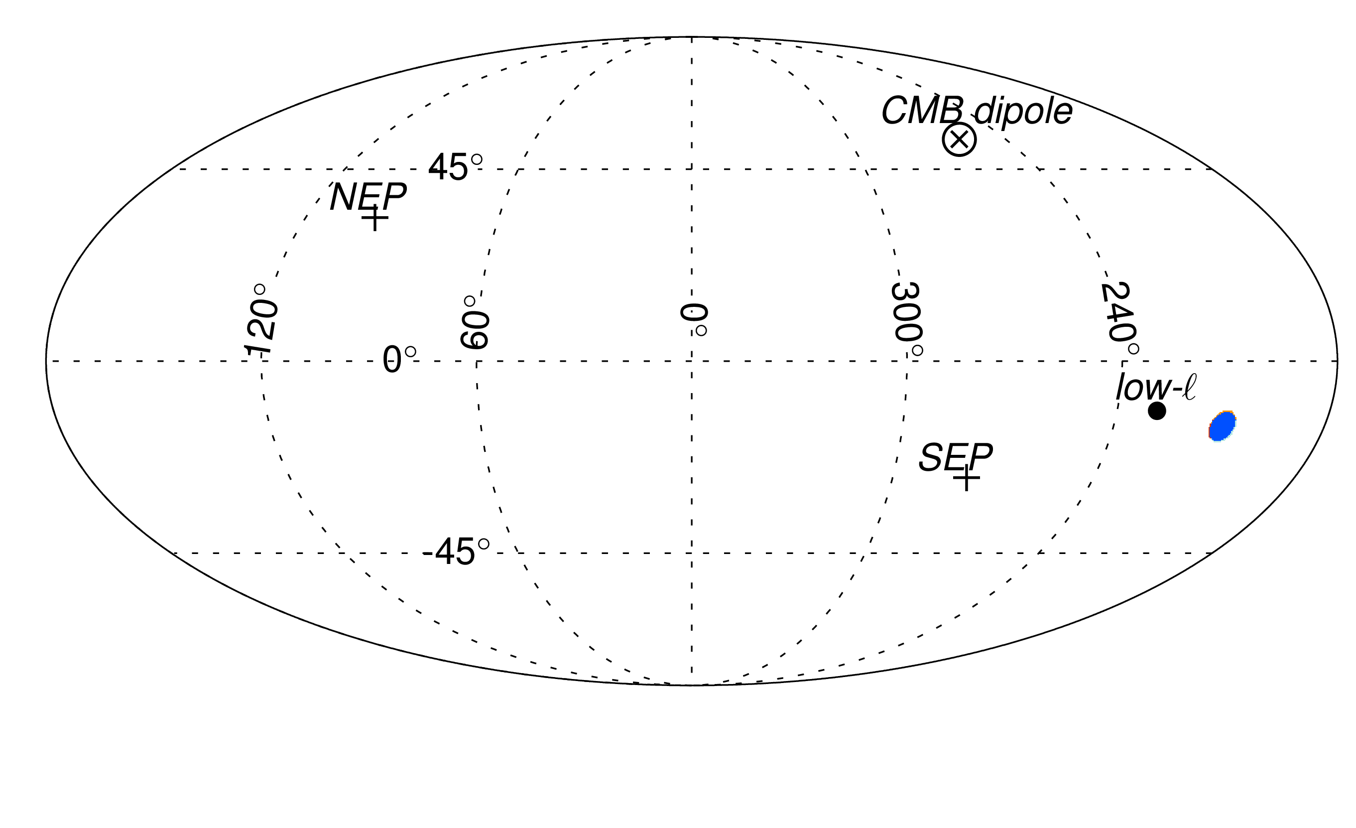
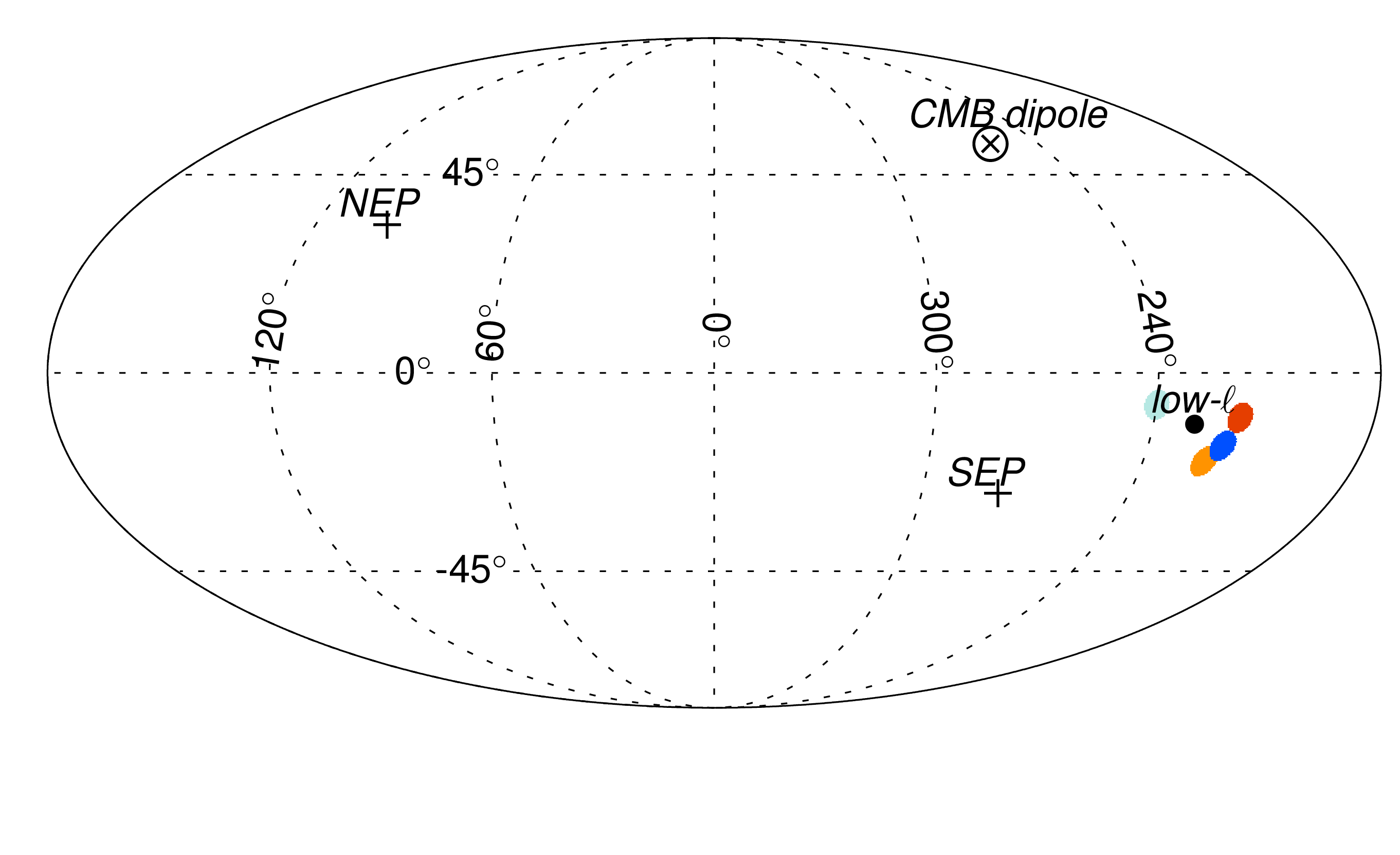
Planck 2018 Planck:2019evm also studied the hemispherical power asymmetry, as well as a few other large-scale anomalies, for the CMB polarization data. By applying the local-variance estimator of Ref. Akrami:2014eta to -mode polarization maps, Planck 2018 found preferred directions for polarization with the smallest -values of and for Commander and SEVEM component-separated maps, respectively, and and for NILC and SMICA, when discs were used. This difference in the significance levels might reflect differences in the component separation approaches, particularly given that the former methods operate in the pixel domain, while the latter in the harmonic domain. Another interesting finding of the Planck 2018 variance asymmetry analysis is that the preferred directions for polarization are intriguingly close to those determined for the temperature data, with the smallest polarization-temperature separation angle of for Commander and SMICA (with -values of ). The preferred directions are and , respectively, which are close to the temperature variance asymmetry direction of for the same and the dipole modulation direction of based on the QML analysis of the 2018 data; see Fig. 20 (right panel). While the differences between the -values and preferred directions associated to the different component-separated polarization maps argue against a detection of cosmological power asymmetry in the polarization data and, therefore, the close alignment of the temperature and polarization directions could simply be a coincidence, future higher-quality polarization data may offer additional insight.
Peak Distribution Asymmetry.
The Planck collaboration employed, in both their 2015 Planck:2015igc and 2018 Planck:2019evm analyses, local extrema (or peaks) in the CMB maps to search for localized anomalies by examining how their statistical properties would vary in patches of the sky as a function of their location. This method was particularly used as a further test for large-scale asymmetries by examining the differences in the peak distribution when divided according to orientation with respect to a previously specified asymmetry direction. In the Planck 2015 analysis, a disc of radius centred on , the dipole modulation direction found in the SMICA temperature map, and its corresponding antipodal disc were used to select the peaks. For maps filtered with a FWHM GAUSS filter, as well as a number of other filtering scales, the distribution of the peaks for the positive-direction disc was in general agreement with the full sky result, while that for the negative direction (close to the northern ecliptic point) was marginally different—this again showed that the northern hemisphere is anomalous. Planck 2018 repeated the analysis using the direction determined by the SMICA QML estimator, , and confirmed the 2015 results.
Predictions.
Limited work has been done to study the predictions of CDM for the wide range of hemispherical power anomalies. However, Ref. ODwyer:2016xov showed that the CDM predictions for the variance in Q and U polarization conditioned on the low northern temperature variance are nearly unchanged from the unconditioned predictions. Any observed suppression of variance in Q and U in the north would therefore be an independent anomaly in CDM, but might be expected in a physical explanation of the temperature anomaly. We expect that similar statements hold for other characterizations of the hemispherical power asymmetry. However, extension of the dipolar power asymmetry signal beyond Aiola:2015rqa ; Shaikh:2019dvb can lead to a power asymmetry in the lensing B-modes of polarization, as shown in Ref. Mukherjee:2015wra . This could be measured from the upcoming ground-based CMB experiments such as SO SimonsObservatory:2018koc and CMB-S4 Abazajian:2019tiv . Other probes such as the kinematic and polarized SZ Cayuso:2019hen can also explore the power asymmetry signal from future surveys. A violation of statistical isotropy can also lead to direction dependence in the inferred cosmological parameters Mukherjee:2015mma . While Ref. Mukherjee:2017yxd concludes that Planck temperature maps do not show any significant departure from statistical isotropy in the inferred cosmological parameters, others Fosalba:2020gls ; Yeung:2022smn claim strong evidence of such variation (see subsection VIII.3.5). In the future, this can be tested using both temperature and polarization data.
VIII.3.3 Quadrupole and Octopole Anomalies
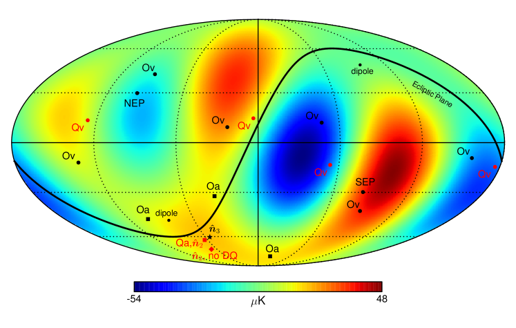
CDM asserts that the are statistically independent random variables. Yet, and show anomalous correlations deOliveira-Costa:2003utu , suggesting .
There are two principal statistical approaches to describing these anomalous correlations. The first is in terms of the multipole vectors of the quadrupole and octopole (Fig. 21): , , . These unit vectors plus a scalar , are an alternative to for representing real scalar functions on the sphere. In CDM, the of different are uncorrelated; the correlations between of fixed are calculable.
It was observed in Ref. Schwarz:2004gk that the oriented areas (normal) of the plane defined by the two quadrupole multipole vectors , and those of the 3 planes defined by the three octopole multipole vectors (), , are unexpectedly close to one another: the magnitude of the dot products of , with the three are approximately , , and . Using instead the themselves and not unit vectors parallel to them, the three dot products are , , and ; in CDM, the p-value of these being at least this large is ! In other words, the three octopole multipole vectors nearly share a a common plane, this is called octopole planarity, and that plane is nearly that of the quadrupole. This is quadrupole-octopole alignment.
The quality of this alignment improved noticeably on removing (as one ought) the Doppler contribution to the quadrupole Copi:2013jna ; Notari:2015kla , reducing the p-value from to the just quoted. This would be a separate ”statistical fluke” in CDM.
The original approach to seeing these alignments was through the angular momentum dispersion in each multipole deOliveira-Costa:2003utu , . The subscript indicates that this is a function of the choice of axis. For each , is the z-axis that maximizes the angular momentum dispersion in that . In the WMAP 1st year ILC map, , which has a p-value of ; this again is quadrupole-octopole alignment. It was noted that in this frame the magnitudes of are much larger than those of other , at a level that has a p-value of 7% in CDM; this is octopole planarity. If the three octopole had been exactly parallel, then they would have been parallel to . This common axis has been called ”the axis of evil” Land:2005jq . Finally, there are some suggestions of correlations also between of pairs of other than and Copi:2003kt ; Land:2005jq .
There are other unexpected correlations of the quadrupole and octopole, in particular with the ecliptic. The great circle defined by the common plane of the quadrupole and octopole is nearly perpendicular to the ecliptic. Near that great circle the quadrupole-plus-octopole combine to produce 6 extrema. The ecliptic great circle seems to trace out surprisingly well the zero separating three strong extrema in the ecliptic south from three weaker extrema in the ecliptic north. This connection to the ecliptic suggests either an experimental systematic or a solar-system foreground. The WMAP and Planck satellites orbited in the plane of the ecliptic and their sampling strategies and noise maps are ”ecliptic-aware,” however their systematics are very different and both see nearly identical quadrupoles and octopoles. As far as solar-system foregrounds, the structure of the quadrupole and octopole as planar and perpendicular to the ecliptic is entirely unlike anything that would be expected from the solar system itself — no reasonable proposal has been made that would generate the observed quadrupole and octopole.
It has been found that if the Universe has non-trivial topology it can induce correlations between the quadrupole and octopole Bielewicz:2008ga , though the statistical evidence for that is weak, and the manifolds specifically consider are ruled out by the search for matched circle pairs Vaudrevange:2012da . In such an explanation, the correlations with the ecliptic would be a fluke.
Predictions.
Because in CDM, the peculiar correlations of the and has little effect on the multipoles of polarization. This may not be the case in specific model explanations of the temperature anomaly. For example, one would expect that in a topologically non-trivial manifold, the boundary conditions would imprint not just on the , but equally on the and . However, the precise prediction is expected to depend strongly on the specific manifold.
VIII.3.4 Point-Parity Anomaly
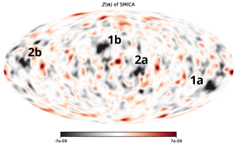
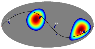
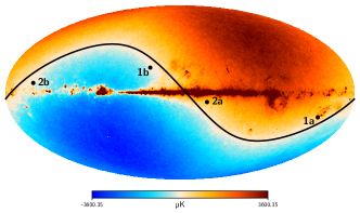
An anomalous power excess of odd multipoles compared to even multipoles has been shown to exist in the CMB angular power spectrum on the largest angular scales () Land:2005jq ; Kim:2010gd ; Kim:2010gf ; Kim:2010st ; Gruppuso:2010nd ; Gruppuso:2017nap ; Planck:2013lks ; Planck:2015igc ; Planck:2019evm . As odd- (even-) spherical harmonics possess odd (even) point-parity, this effect is known as the point-parity anomaly.353535Note that this is different from the so-called ”mirror-parity anomaly”, which is about the properties of the CMB maps under reflection with respect to a plane. Both Planck 2013 Planck:2013lks and Planck 2015 Planck:2015igc reported evidence for an anti-symmetry plane in low-resolution temperature maps with the direction and a -value ranging from to depending on the component separation method. The analysis of the higher-resolution maps showed almost the same direction, , with lower -values ( to ). This mirror-parity anomaly was first detected in the WMAP 7-year data Finelli:2011zs , with an anti-symmetry direction almost identical to the one found by Planck, which is within of the dipole modulation direction.
In order to compare even and odd multipoles, Ref. Kim:2010gf considered the parity asymmetry statistic , where and are the mean power in even and odd multipoles respectively for the range ,
| (131) |
The CDM model predicts , i.e. . Examining WMAP3 and WMAP5, Ref. Kim:2010gf found that for up to , with a -value in CDM of .
The point-parity anomaly was re-examined in Refs. Aluri:2011wv ; Hansen:2011wk ; Kim:2012hf ; Gruppuso:2010nd ; Kim:2010gd using the 5-year and 7-year releases of WMAP data. Ref. Aluri:2011wv found that the anomaly extended out at least to . Focusing on the power spectrum in the domain, an excess of oddness with significance was found, which was related to the correlation function at large angular scales Kim:2012hf . The point-parity anomaly persists in the Planck temperature data Planck:2013lks ; Planck:2015igc ; Planck:2019evm ; Gruppuso:2017nap ; Shaikh:2019dvb with the lowest -values of found at .
Recently, properties of the point-parity asymmetry were investigated directly for SMICA CMB map pixels to identify the preferred directions on the sky responsible for this type of anomaly Creswell:2021eqi ; Creswell:2021xzf . The method proposed in Refs. (Creswell:2021eqi, ; Creswell:2021xzf, ) is based on the signal symmetry properties at each pixel and its anti-pode with respect to the center of the map: , where the symmetric () and asymmetric () parts of the temperature anisotropy map are
| (132) | |||||
| (133) |
Here is a unit vector pointed to each pixel of the map. Following Refs. Creswell:2021eqi ; Creswell:2021xzf , one can define the estimator of symmetry or asymmetry of the temperature map for each pixel,
| (134) |
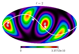
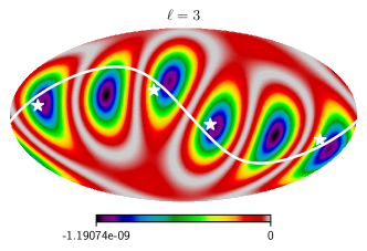
Thus, if , then the symmetric component dominates the asymmetric component, and vice versa. In Fig. 22 we plot maps derived from the Planck 2018 SMICA map with Gaussian smoothing Creswell:2021eqi ; Creswell:2021xzf . An important feature visible in Fig. 22 is the two pairs of very strong high negative peaks of , labelled by 1a/1b and 2a/2b (a and b of each pair are antipodal from one another), and about ten negative peak-pairs with smaller amplitudes, mainly localized within the area in Galactic coordinates. These highest peaks (1a/1b and 2a/2b) with belong to the asymmetric component of the signal and have the following Galactic coordinates :
| (135) | ||||
| (136) |
Peaks 1a/1b lie outside the area of the Union mask smoothed by a Gaussian filter with , while peaks 2a/2b are inside this masked area.
The most powerful negative peaks 1a/1b and 2a/2b are located along the kinematic dipole percolation line, where and are polar and azimuthal coordinates Creswell:2021eqi ; Creswell:2021xzf . The kinematic dipole is a well-known non-cosmological component of the CMB signal induced due to the motion of the solar system with respect to the rest frame of the CMB radiation. Observations from COBE, Planck and WMAP give a direction of the kinematic dipole of (Planck 2015 nominal) and (WMAP) in the Galactic coordinates (Planck:2015mrs, ; WMAP:2010sfg, ). Denoting this direction with the unit vector , we introduce the concept of the ring of attraction (RA) including all directions such that i.e. are all unit vectors orthogonal to the direction of the kinematic dipole . Fig. 23 shows that RA includes the directions of not only the 1a/1b and 2a/2b parity peaks but also the CMB dipole modulation used in Refs. Planck:2013lks ; Planck:2015igc ; Planck:2019evm to explain the power asymmetry. Analysis of the random simulations for the multidirectional dipoles shows that the coincidence of the point-parity peaks and the power asymmetry direction shown in Fig. 23 is represented in one of the 2000 realizations.
The presence of RA can also be seen in the Z-maps for the quadrupole and CMB octopole shown in Fig. 24. For the quadrupole, the two highest positive peaks coincide with the position of peaks 2a/2b from Fig. 22, while for the octopole Z-map all peaks 1a/1b, 2a/2b coincide with the position of the deepest negative peaks. Overall, the above results might suggest a causal relationship between kinematic dipole, parity anomaly, CMB spectrum power asymmetry and quadrupole and octopole features, motivating more detailed studies of the systematic and calibration effects of CMB data. It is, however, important to note that while the connection to the CMB dipole direction (or the ecliptic pole) would suggest a possible systematic, there is no known common systematic in WMAP and Planck. Similarly, there is no known foreground that could be responsible for a connection to the CMB dipole. Additionally, if the signal is dominated by a systematic or foreground, then this suggests that the underlying cosmological signal is even smaller, exacerbating the lack of large-angle correlations.
VIII.3.5 Variation in Cosmological Parameters Over the Sky
Several attempts have been made to assess whether CDM parameters are homogeneous and isotropic, as FLRW cosmology assumes. (See, for example,Axelsson:2013mva ; Mukherjee:2015mma ; Mukherjee:2017yxd ; Yeung:2022smn ; Camacho-Quevedo:2021bvt .) Given the statistically significant violations of statistical isotropy described above, one might wonder whether the differences in parameters estimated from different parts of the Universe are consistent with the expected variation in perturbed-FLRW.
A recent analysis Fosalba:2020gls of the Planck legacy temperature maps, considering , finds evidence for a violation of statistical isotropy. Three patches of the sky in angular diameter, over each of which the the CDM parameters are approximately homogeneous, exhibit sizable differences between one another. For example, ranges from to ; ranges from to . This level of variation exceeds that in any of the 300 realizations of CDM to which they compare, though the authors calculate that the discrepancy has a probability of being a statistical fluctuation in CDM. The authors note that these patches subtend the same angular scale () above which is unexpectedly close to zero (see Sec. VIII.3.1 above). They are also comparable in size to the patterns of the quadrupole and octopole, which are anomalous (see Sec. VIII.3.3).
The authors connect the size of these patches to the size of the anti-trapped surface (causal horizon) due to , , placed at the last scattering surface. They suggest that the underlying physical mechanism sourcing the observed temperature anisotropies therefore encompasses scales beyond our causal Universe. The authors argue that these well-defined regions may reflect casually disjoint horizons across the observable Universe. They show that, within each patch, the observed relations between its size and the mean value of the dark-energy density or are in good agreement with expectations from a recently proposed model of the Universe Gaztanaga:2020ksy ; Gaztanaga:2021bgb ; gaztanaga:hal-03344159 ; Gaztanaga:2022 .
The possible existence of similar horizons in the local Universe could provide a simple explanation for the claimed cosmological parameter tensions between the low and high redshift Universe. Future Surveys such as Rubin/LSST, Euclid, and Roman will map similar scales at .
More recently, similar conclusions have been arrived at independently in Ref. Yeung:2022smn by using hemispherical masks and fitting the Planck temperature angular power spectrum for 48 directions on the sky. It is found that the directional dependences of the cosmological parameters follow a dipole to good approximation and that the Bayes factor strongly disfavours an isotropic Universe. The reported dipole is roughly perpendicular to the fine structure dipole and within of the directions corresponding to the CMB kinematic dipole, the CMB parity asymmetry dipole, and the axis in QSO polarizations. The Hubble constant varies between and across the sky.
VIII.3.6 The Cold Spot
The cold (blue) spot was first found in WMAP 1-year temperature data by Ref. Vielva:2003et and was confirmed in Planck data Planck:2013lks ; Planck:2015igc ; Planck:2019evm in the southern hemisphere at the galactic longitude and latitude . It is a statistical anomaly of the large-angle fluctuations in the CMB indicating non-Gaussian features. The cold spot is an unusually large region of low temperature with the mean temperature decrease and is in disagreement with the prediction of Gaussianity of the standard CDM model Cruz:2004ce ; Cruz:2006sv ; Cruz:2006fy . Its significance is - depending on the statistical method applied Zhang:2009qg ; Nadathur:2014tfa ; Kovacs:2017hxj . The inconsistency with Gaussian simulations has a -value of Cruz:2009nd . The anomalous nature of the cold spot corresponds to a rather cold region with an angular radius in the sky of about from the centre surrounded by a hot ring Zhang:2009qg ; Nadathur:2014tfa ; Kovacs:2017hxj .
The origin of the cold spot anomaly could be due to the following effects: non-Gaussian feature due to a large statistical fluctuation Vielva:2003et , an artifact of inflation Cruz:2004ce , the foreground contamination Cruz:2006sv ; Hansen:2012xq , the multiple voids Naidoo:2015gab , the imprint of a supervoid (about Mpc radius completely empty void at ) through the ISW effect Inoue:2006rd ; Inoue:2006fn ; Rudnick:2007kw ; Granett:2008ju ; DES:2021cge ; Masina:2008zv ; Masina:2009wt ; Masina:2010dc , the axis of rotation of the Universe Jaffe:2005pw , the cosmic texture Cruz:2004ce ; Zhao:2012hz and the adiabatic perturbation on the last scattering surface Valkenburg:2011ty (see Refs. Cruz:2009nd ; Vielva:2010ng for reviews).
VIII.3.7 Explaining the Large-Angle Anomalies
The apparent connection of certain anomalies to the ecliptic plane (quadrupole-octopole, hemispherical asymmetry) – which certainly has no role in a theory of cosmology – suggests a local origin. However, the large angle anomalies are extremely difficult to ascribe to the usual suspects: experimental systematics and foregrounds.
The systematic effects of both WMAP and Planck T measurements are thought to be well in hand at low-, especially outside the Galactic plane. Moreover the experiments have very different observational strategies and it would be very surprising for them to independently generate the same set of anomalies, especially with such remarkable agreement.
A foreground typically adds a signal with its own correlations to the underlying cosmological signal. It would be challenging for a foreground to suppress angular correlations on large angles, or to reduce the variance in the fluctuations over half the sky. If the peculiar quadrupole and octopole are due to a foreground, then that foreground signal is on top of an even more highly suppressed cosmological quadrupole, and the magnitude of the underlying cosmological angular correlation function is even smaller. Any ”cancellation” would itself be a fluke. The spatial structure of the quadrupole and octopole – essentially a ring of extrema perpendicular to the ecliptic plane – make them particularly difficult to explain through foreground. It is not easily mapped into any feature of the solar system, nor of the galaxy. Explanations of quadrupole-octopole alignment that produce aligned and – say from an unusual patch of foreground – are irrelevant. Explanations that are perturbative in some small quantity, must explain why , rather than .
Microphysical explanations are also challenging. Changes in the inflationary potential will change the power spectrum of fluctuations, but will not induce correlations between . Similarly, changes in the growth of fluctuations. Changes to the propagation of photons will not correlate s, unless it is the underlying propagation physics that itself is modulated, and even then will superpose some new signal on top of the ”original” cosmological signal, not a tabula rasa.
An attempt to ascribe the absence of large angle correlations (low ) to an absence of long distance correlations – by replacing Fourier modes with wavelets Copi:2018wsv , could suppress , but not , and so not .
The most promising idea appears to be that the anomalies are induced by horizon-scale or super-horizon-scale properties of cosmic geometry, for example by non-trivial spatial topology. Spatial topology changes the boundary conditions of wave operators. Their eigenspectra are altered, as are their eigenmodes. Specifically, radial functions times individual spherical harmonics are no longer eigenmodes, and so even though the background metric may remain homogeneous and isotropic, statistical isotropy is broken and , as required for any explanation for the anomalies. (Non-FLRW metrics would change the differential operators themselves, and would have similar consequencesMcEwen:2013cka .)
A number of preliminary attempts Aurich:2007yx ; Bielewicz:2008ga ; Aurich:2012jc ; Aurich:2014sea ; Bernui:2018wef have been made to explore the potential for topology to explain the anomalies – with some success in reproducing the quadrupole-octopole structure Bielewicz:2008ga and low Aurich:2007yx , without suppressed Bernui:2018wef . However, the specific topologies considered run afoul of existing limits on topology from the absence of pairs of circles on the CMB sky with matched patterns of fluctuations Cornish:1997ab ; Cornish:2003db ; ShapiroKey:2006hm ; Vaudrevange:2012da ; Planck:2013okc ; Planck:2015gmu (widely accepted despite the claims in Refs. Aurich:2007yx ; Aurich:2014sea ), and from comparisons to the predicted two-point correlations of specific topologies (with fixed values of certain free parameters) Aslanyan:2013lsa ; Planck:2013okc ; Planck:2015gmu . More work to search for topology and explore its potential connection to CMB anomalies is ongoing.
VIII.3.8 Predictions and Future Testability
The key to establishing whether the observed large-angle anomalies are statistical flukes or exciting evidence for new physics is to identify testable predictions for properties of the CMB polarization, large scale structure, or other cosmological observables. As discussed above, predictions come in three types: predictions of CDM, conditioned on the existing temperature maps (or on summary statistics of those maps); generic predictions expected of physical explanations, but not tied to a specific model; predictions of specific models to explain specific anomalies. To date, there are no specific models for which such predictions have been made.
We summarize what was written above regarding each anomaly.
CDM Conditional Predictions.
Largely because the correlation between temperature and polarization is weak in CDM (, ), CDM conditional predictions for polarization are nearly indistinguishable from unconditioned predictions. Similar statements likely hold for predictions for other observables such as large-scale structure, lensing, other secondary CMB anisotropies, 21cm and other intensity fluctuations, and so on. This is actually a useful state of affairs because it allows us to test the fluke hypothesis (that anomalies are statistical accidents in CDM) by searching for analogous anomalies in these other observables. Which anomalies are most amenable to this approach is perhaps best guided by expectations from the generic predictions expected of physical explanations, but not tied to a specific model (see below).
What can change significantly is predictions for correlations between temperature and other observables, e.g. Ref. Yoho:2013tta for the temperature-lensing-potential two-point correlation function . Here one finds that the peak of the distribution of in constrained realizations is reduced by a factor of approximately compared to unconstrained realizations. Nevertheless, a value of far into the low tail of the PDF for unconstrained realizations will still be in the low tail of the PDF for constrained realizations. Similar analyses should be performed for cross correlations of CMB with other signals that are sensitive to high redshifts (though still with ).
Generic Predictions Expected of Physical Explanations.
Even in the absence of a specific model, one can put forward certain reasonable expectations of a physical explanation for the anomalies:
-
•
The low value of will result in a low and . There is a weaker expectation for a suppressed value of of local-E polarization Yoho:2015bla , because it is dominated by higher- modes; there is no clear expectation value of properties of non-local versions of the pseudo-field E.
-
•
The low value of implies Copi:2013cya a low Doppler-subtracted (i.e. intrinsic) dipole .
-
•
The hemispherical asymmetry in implies a similar asymmetry for , , (local), and perhaps . This should perhaps best be viewed as a low variance in those quantities in the northern (approximately ecliptic) hemisphere.
Generic Predictions Expected of Specific Models.
Specific choices of topology have been argued to potentially explain low or quadrupole-octopole correlations. However, these specific topologies appear to violate known limits. Some physical models that seek to explain the apparent violation of statistical isotropy observed in T, may also predict independent statistical isotropy violation in polarization of the CMB (i.e. that is not a direct consequence of the observed temperature sky), which could be detected in future polarization data Mukherjee:2014lea ; Mukherjee:2015wra ; Cayuso:2019hen .
Future Tests.
We have have identified three specific tests of the fluke hypothesis that are also motivated by expectations for explanations through new physics:
-
•
Measurement of and , as well as and Yoho:2015bla . This would require improvements on Planck for large-angle correlations in polarization through an all-sky experiment.
-
•
Measurement of the cosmological contribution to , by subtraction of the Doppler contribution to . This requires sub-percent-accuracy determination of our velocity relative to the CMB rest frame from mixing between high- multipoles, enabling the Doppler contribution to to be subtracted from a similarly accurate direct measurement of . This would require improvements on Planck for high .
-
•
Measurement of the variance in , , and in the northern hemisphere ODwyer:2016xov ; CMB-S4:2016ple . This would require improvements on Planck for large-angle correlations in polarization over a large fraction of the north-ecliptic hemisphere, as well as an improved independent determination of the optical depth to reionization ODwyer:2019rfg .
VIII.3.9 Summary
There are multiple anomalies on large angular scales in the CMB temperature maps. Each is of significance, each is characterized with a posteriori statistics, but several sets of anomalies are statistically independent (or nearly so) in standard CDM. Collectively they are very troubling. They are common to WMAP and Planck (and COBE), so difficult to explain by unaccounted-for observational systematics. They are unexplained by known foregrounds, and a foreground explanation would itself imply an (even more) highly suppressed large-angle cosmological signal.
For several anomalies, one anticipates that a physical explanation would imply an analogous anomaly in the scalar (E-mode) contributions to Q and U polarization, and perhaps in the tensor (B-mode) contribution as well. Similar statements may be applied to other probes of the large-scale Universe – e.g., intensity maps, surveys of large scale structure – but the expectation is weaker. Meanwhile, CDM predictions for polarization (and late-time observables) are nearly unchanged by conditioning on the observed temperature maps, therefore only cross-correlations with temperature are significantly altered.
Large-angle properties of the CMB should be a matter of continued attention for the experimental and theoretical cosmology communities. Conditional predictions in CDM, provide accessible null tests of CDM through improved measurements of polarization on large angular scales, of improved determination of our velocity relative to the CMB, and possibly through large angle/distance auto and cross correlations between observables including those probing moderate redshift. The existence of reasonable expectations for physical models, suggest opportunities to provide compelling evidence for fundamentally important new physics. Non-trivial cosmic topology or anisotropic geometry are the only current promising frameworks for a comprehensive explanation; these should be more thoroughly explored.
VIII.4 Abnormal Oscillations of Best Fit Parameter Values
Signature of an oscillation, or unusual behavior of the data around the best fit CDM model have been reported in Refs. Riess:2017lxs ; Colgain:2019pck ; Camarena:2019moy ; Kazantzidis:2020tko ; Sapone:2020wwz ; Dainotti:2021pqg . These signatures were mainly found using the binned Pantheon data. However, assigning significance to such oscillations in the data in the residual space around a best fit model requires a large number of simulations. One should note that different realizations of a data based on the same covariance matrix given a specific model would differ from each other and in some particular realizations we might see some specific features. Hence to assign a reliable statistical significance to any specific feature beyond expectations of a given model or hypothesis, we need to generate a large number of Monte Carlo simulations and see how often we might observe such or similar features. We should also consider a ”look elsewhere effect” that features due to random fluctuations might occur at different parts of the data and not necessarily at a specific range of the data. Following this approach, Ref. Kazantzidis:2020xta generated 1000 realizations of the Pantheon supernovae data and evaluated how likely it is to observe the oscillations we see in the Pantheon real data around the best fit CDM model. Considering the full covariance matrix of the data taking into account both systematic and statistical uncertainties, they did show that at the redshifts below such oscillations can only occur in less than of the simulations. While statistical fluctuations can be responsible for this oscillation, this could also be a hint for some feature beyond the expectations of the standard model. Alternatively this could be a hint for some specific systematics in the data. More observations would make it soon clear if the observed effect is due to statistical fluctuations or there is some real physics or systematics behind such apparent behavior.
VIII.5 Anomalously Strong ISW Effect
The decay of cosmological large-scale gravitational potential causes the integrated Sachs-Wolfe (ISW) effect Sachs:1967er which imprints tiny secondary anisotropies to the primary fluctuations of the CMB and is a complementary probe of dark energy, e.g. Ref. Fosalba:2003iy . Using a stacking technique Marcos-Caballero:2015lxp ; Planck:2015igc in the CMB data, an anomalously strong integrated Sachs–Wolfe (ISW) signal has been identified for supervoids and superclusters on scales larger than at a level Granett:2008ju ; Granett:2008xb . This stronger than expected within standard CDM signal of the ISW effect first emphasized in Ref. Hunt:2008wp has been studied by Refs. Nadathur:2011iu ; Flender:2012wu ; Ilic:2013cn ; Cai:2016rdk ; Kovacs:2017hxj ; Kovacs:2018irz ; Dong:2020fqt .
In particular, the analysis by Ref. Kovacs:2018irz for DES data alone found an excess ISW imprinted profile with amplitude (where the value corresponds to the CDM prediction). A combination with independent BOSS data leads to , in tension at with the predictions from CDM cosmology. The average expansion rate approximation (AvERA) inhomogeneous cosmological simulation Racz:2016rss indicates under the inhomogeneity assumption, about times higher ISW effect than CDM depending on the index of the spherical power spectrum Beck:2018owr . Thus the large scale spatial inhomogeneities may be the plausible sources of this ISW excess signal. Using angular cross-correlation techniques Ref. Giannantonio:2012aa combines several tracer catalogues to find . In addition the early Integrated Sachs-Wolfe (eISW) effect Bowen:2001in ; Galli:2010it () has been studied by Refs. Hou:2011ec ; Cabass:2015xfa ; Kable:2020hcw ; Vagnozzi:2021gjh and constraints were imposed on the corresponding parameter . In general, the reported amplitude varies in the literature depending on the dataset and the assumptions of the analysis. Further investigation of this issue is needed.
VIII.6 Cosmic Dipoles
There have been claims of signals indicating the violation of the cosmological principle. Some of these signals coherently point to the CMB dipole direction, which is assumed to be of purely kinematic origin. Some of the dipoles have different directional dependence, and for these observations, there is no obvious pattern. A physical mechanism for producing such violation on Hubble scales is studied in Ref. BuenoSanchez:2011wr . See also Sec. VII.8.2 for an introduction to the mapping of anisotropies in cosmological observables in general space-times without exact symmetries. The dipolar signals found include the following:
VIII.6.1 The Dipole
Measuring from Quasar Spectra.
High resolution spectra of distant quasars reveal numerous narrow absorption lines due to gaseous components of galaxies intersecting the Earth–quasar line of sight. The large number of atomic species and transitions detected allow precise measurements of the fine structure constant over cosmological distances, where is the electron charge, the vacuum permittivity, the reduced Planck constant, and the speed of light. The dimensionless is the ratio of the speed of an electron in the lowest energy orbit of the Bohr-Sommerfeld atom to the speed of light, and hence connects quantum mechanics (through ) with electromagnetism (through the remaining constants in the ratio).
The 1999 invention of the Many Multiplet method (MM) Dzuba:1999zz provided an instant order of magnitude precision gain over previous methods in searches for space-time variations of . This is because the difference between ground-state and/or excited state relativistic corrections can be large; – and – transitions for example may even be of the opposite sign. The MM method can thus produce sensitive results when applied simultaneously to multiplets of the same atomic species, or to species having widely differing atomic masses. Any real change in therefore generates a unique pattern of observed wavelength shifts that is not degenerate with a simple redshift.
In parallel with the development of the MM method, its first application to high-resolution quasar spectra from the HIRES spectrograph on the Keck telescope was reported in Ref. Webb:1998cq and suggested a possible variation. The acquisition of several further quasar samples, initially from the Keck telescope Webb:2000mn ; Webb:2002vd ; MurphyPhD2002 ; Murphy:2003hw , also suggested variations and led ultimately to the extensive study carried out using the UVES spectrograph on the VLT, reported in Refs. Webb:2010hc ; KingPhD2011 ; King:2012id . The combined Keck and VLT samples comprised 293 independent measurements of the fractional change , where is the value of the fine structure observed in a gas cloud at redshift and is the terrestrial value. These 293 measurements cover both hemispheres and span a redshift range of , permitting a search for temporal and spatial variations of .
The main outcome of the detailed 2011 study by King, Webb, and collaborators is the intriguing hint of a spatial variation of the electromagnetic force, consistent with an angular dipole model pointing in the direction RA , dec , with amplitude . A bootstrap analysis showed a dipole model was preferred over a simple monopole model at the level. The apparent dipole was captivating for several reasons: first, measurements made at lower redshift use a different set of atomic transitions to those at higher redshift, yet both measurements independently support a dipole. Second, the independent Keck and VLT samples both suggest a dipole effect, again along the same direction and with consistent dipole amplitudes. Despite these apparent coincidences, it should be noted that measurement uncertainties for subsets of the whole sample are large and not individually significant. A reasonable statistical significance is only seen when the whole sample is modelled simultaneously.
Ref. Berengut:2010yu made use of the 2011 King et al data to further examine the properties of the dipole model and to explore the possibility of detecting dipoles in measurements of variation in electron-to-proton mass ratio , combinations of fundamental constants such as (where is the proton g-factor), and big bang nucleosynthesis probes of the baryonic density parameter using measurements of the primordial deuterium abundance, D/H. Since the number of , , and D/H measurements has increased only slightly, little has been done on those dipole studies since the analysis in Ref. Berengut:2010yu .
Detailed studies have also been done to check whether may change in strong gravitational fields Berengut:2013dta ; Bainbridge2017a ; Bainbridge:2017lsj ; Hu:2020zeq . For some white dwarfs, where physical conditions permit, many narrow photospheric absorption lines are detected. The large number of Fe v and Ni v transitions are particularly useful since they have a broad range of sensitivities to , so that (as with quasar measurements) any change in does not emulate redshift. At present, the most detailed analysis to date gives a best result of , so there is no clear evidence for a change in . Although the quality of the astronomical data is high (indicated by ), results are currently severely constrained by the precision of laboratory wavelengths used to compare with the detected lines, the dominant part of Hu:2020zeq . Significant improvements in the laboratory wavelength measurements are needed to make further progress.
Overcoming the Systematics.
An early list of potential systematic effects associated with measurements is given in Ref. Murphy:2000pz ; Murphy:2002ve although the subject has moved on since that time. We now have a considerably better understanding of systematics and new mathematical/statistical tools have been developed to identify and quantify them. An exhaustive discussion of systematics is not appropriate here so instead a precis of four important effects is given. The first two are essentially solved problems (but exist in previously published surveys) whilst the second two are not yet solved.
Non-uniqueness in absorption system modelling: It has long been recognised that a complex quasar absorption system can be modelled in essentially an infinite number of ways. However, interactive model fitting is a laborious process such that it is impractical to construct more than a single model for an absorption system in most cases. To constrain model options to some extent, a common approach is to gradually increase the number of model parameters until the model matches the data with a normalised of around unity. Although the method is reasonable and has been widely used, it is not the best approach, so Ref. King:2012id employed an information criterion (IC) to optimise the number of model components. Whilst using an IC strikes a balance between fitting too few and too many parameters, different humans modelling the same data will usually derive slightly different models, each with a slightly different value of . From the point of view of understanding systematics, the important question then becomes, how different? This ”non-uniqueness” problem has very recently been solved. A new ”Artificial Intelligence” approach was introduced that completely removes human decision making (and time commitment) from the modelling process Lee:2020lof . This enables a Monte Carlo approach to modelling, emulating multiple interactive modellers. Computations are intensive but manageable using high performance computers. In conjunction with those advances, a new spectroscopic IC has been developed specific to spectroscopy, that appears to improve on previous statistics 2021MNRAS.501.2268W . The three developments just described enable us to quantify, for the first time, the effect of non-uniqueness on measurement uncertainty Lee:2021kjr . To summarise, the issue of model non-uniqueness is now a solved problem, provided that AI Monte Carlo (or something equivalent) is used to derive a sample of models for each absorption system being measured.
Wavelength calibration problems: Ref. Molaro:2007nm first searched for wavelength distortions in high-resolution echelle spectra by correlating the reflected solar spectrum from VLT/UVES asteroid observations with absolute solar calibrations but found no evidence for long-range wavelength distortion. Subsequently, Ref. Rahmani:2013dia applied the same technique and indeed found that long-range wavelength distortions do occur in UVES spectra. The form of the distortion appears to be reasonably well approximated by a simple linear function of velocity shift versus observed wavelength. Ref. Whitmore:2014ina examined the problem in further detail confirming problem. They then attempted to estimate the impact of this distortion effect on possible dipole but did not take into account the considerably more complex distortion that would apply to a quasar spectrum formed from the co-addition of multiple exposures at the telescope, some or all having different instrumental settings. That problem was resolved in Refs.Dumont:2017exu ; 2021MNRAS.508.3620W , such that any possible long-range distortion VLT/UVES and Keck/HIRES spectra can be allowed for, as discussed in detail in Ref. Lee:2021kjr ; future measurements made using archival UVES and HIRES spectra should in principle be unbiased and the total error budget realistic.
Considerable effort has gone into wavelength calibration of the new ESPRESSO spectrograph (Echelle SPectrograph for Rocky Exoplanets and Stable Spectroscopic Observations) on the VLT 2020PhDT……..13M ; Milakovic:2020ehq ; 2020NatAs…4..603P . In particular, laser frequency combs (LFCs) and Fabry-Pérot devices produce ESPRESSO calibrations down to an accuracy of m/s Schmidt:2020ywz . In principle the accuracy should be somewhat better than this value (and indeed 1 limit of 1-2 m/s has been reached for the High Accuracy Radial Velocity Planet Searcher (HARPS) instrument). Further work is anticipated. A limiting value of 24 m/s corresponds to an uncertainty of on .
Magnesium isotopes: The Mg ii 2796/2803 doublet is often strong in quasar absorption systems and is relatively insensitive to variation. For these reasons, it was introduced as an ”anchor” against which to measure relative shifts of more sensitive species such as Fe ii Webb:1998cq . However, the low atomic mass of Mg means isotopic and hyperfine separations are non-negligible in the context of varying measurements. Therefore, if we fit high redshift absorption lines using models that assume terrestrial isotopic abundances, and if relative isotopic abundances in quasar absorbers are not terrestrial, this may mimic a change in , as first pointed out in Ref. Webb:1998cq . Further discussions on this systematic are given in Refs. Murphy:2000pz ; Murphy:2002ve ; Kozlov:2004fc ; Ashenfelter:2004kk ; Fenner:2005sr ; Agafonova:2011sp ; Berengut:2011hsa ; Webb:2014lpa ; Vangioni:2018zef . This is an unsolved problem in the sense that the Mg relative isotopic abundances at high redshift are not yet well-determined, nor whether they may vary significantly from one quasar absorber to another. Despite that, this systematic is straightforward to quantify simply by treating the Mg isotopic abundances as unknown variables to be solved for in conjunction with modelling for (the obvious penalty being a slightly weaker constraint on ). Of course, Mg is not the only element with this potential problem although it is perhaps the most important in the context of measurements.
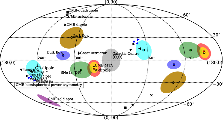
Instrumental profile: It is known that the intrinsic instrumental profile (IP) of the ESPRESSO instrument varies as a function of detector position and wavelength 2020PhDT……..13M ; Milakovic:2020ehq . Since Voigt profile models must be convolved with the IP during the modelling process, it is imperative to have an accurate model of the IP. This problem has not yet been fully solved although numerical and analytic approximations have been made and help. A detailed study for HARPS 2021A&A…645A..23Z has been carried out but not yet for ESPRESSO.
Current Status of the Dipole.
IR spectroscopy of very high redshift quasars allow us to extend the cosmological volume of the 2011 measurements described above. At the time of writing, only one quasar spectrum obtained using the X-SHOOTER spectrograph on the VLT has been analysed, the quasar J1120+0641 Wilczynska:2020rxx . The achievable spectral resolution is at present that of e.g. UVES/VLT and that of ESPRESSO/VLT. Whilst the X-SHOOTER error bars are substantially larger than the higher resolution HIRES/Keck or UVES/VLT data, at the high redshift end, these IR data are the best presently available and contribute 4 new measurements, increasing the sample size very little but significantly augmenting the redshift range to .
Further contributions come from measurements by Molaro and collaborators using UVES on the VLT. The Molaro team concentrated efforts on a small number of high signal to noise spectra, in order to reduce the statistical uncertainty. That sample of 21 measurements has been published in 10 papers and is summarised, with citations, in Table 1 of Ref. Martins:2017qxd . Additionally, another UVES/VLT sample of measurements are reported in Ref. Wilczynska:2015una , forming a combined total set of 323 measurements. As reported in Ref. Wilczynska:2020rxx , these additional measurements allow us to update the spatial dipole parameters: the updated dipole amplitude is and the dipole sky location is right ascension hours and declination . For that analysis, a dipole is preferred over a simpler monopole model at the 3.9 level. On the other hand, an independent analysis of essentially the same dataset as in Ref. Martins:2017qxd , using a different type of analysis (likelihood with marginalisation over certain parameters), arrives at a lower dipole significance level of 2.3. Given the similarity between the samples used by both groups, the origin of the difference between these significance levels is unclear. However, the error budget in a recent dipole estimate Wilczynska:2020rxx incorporates, in addition to the standard statistical uncertainty, an allowance for an ”unknown” systematic (as described in section 3.5.3 of Ref. King:2012id ) and an additional uncertainty associated with possible long range distortion (even though none was found). The error estimate in Ref. Wilczynska:2020rxx is thus cautious, we are aware of no reason to think it unreliable, and suggest that measurement is the most reasonable. Whether a dipole will persist in new and forthcoming ESPRESSO/VLT spectra remains to be seen. Data is now beginning to accumulate in the ESO archive and new measurements using that higher quality data are underway.
The purpose of explaining at least some of the systematics associated with varying measurements above was to highlight the importance of fully resolving those issues in order to facilitate rigorous tests of variation, be they spatial or temporal. The tentative dipole cannot be meaningfully tested until these issues are dealt with. Concerted efforts have been made, notably the development of AI-VPFIT, the new information criterion SpIC, detailed studies about model non-uniqueness, as well as extensive investigations into wavelength calibration, explicitly to be able to move ahead with stringent tests of variation. A complete re-analysis of virtually all existing quasar absorption measurements will soon be completed, together with new measurements from ESPRESSO. Finally, a number of possible anisotropic effects from a broad range of observations have been reported in the literature and are illustrated in the all-sky plot shown in Figure 25.
Theoretical context.
Theoretical models incorporating either temporal or spatial variations of fundamental constants require physics beyond General Relativity and hence beyond the standard FLRW cosmological model. Given the broad landscape of possible varying constant theories, the association between variations and the cosmological tensions reported extensively in this article is, as yet, undetermined. A generalised theory of varying (Barrow:2011kr, ) has been developed in which electromagnetism varies with the chamelionic scalar field potential via a variable coupling constant , the latter being constrained by quasar absorption observations. This theory extends the Bekenstein and Sandvik BSBM theory (Sandvik:2001rv, ; Magueijo:2002di, ) in which the observationally constrained coupling parameter does not depend on . A further BSBM extension shows that if the kinetic energy in the scalar field drives the acceleration of the expansion, need not asymptote to a constant value at the present epoch (Graham:2014hva, ). If so, this motivates further precision increases in laboratory experiments to measure the time dependence of (Leefer:2013waa, ). Various kinds of spatial variations in physics (i.e. not just fundamental constants) have been explored. For example Audren:2014hza examine a quantum gravity scenario in which a preferred time-direction occurs at each point in space-time, parameterised by a vector field coupled to dark matter. The same model could also explain spatial variations in fundamental constants. Interesting coincidences between different types of possible anisotropic phenomena have been pointed out in Mariano:2012wx (also see Figure 25 for a compilation of various claimed dipole effects). C. Martins and colleagues have explored a range of theoretical ideas showing how constraints on temporal or spatial variation of the fine structure constant provides important new requirements for dark energy models. Recent discussions from that group are given in Leite:2017zmo and in Martins:2017yxk .
There are also interesting ideas about extreme fine tuning of quantum corrections in theories with variation of by O’Donoghue Donoghue:2001cs and Marsh Marsh:2016ynw . Self-consistent theories of gravity and electromagnetism, incorporating the fine structure constant as a self-gravitating scalar field, with self-consistent dynamics that couple to the geometry of spacetime, have been formulated in Refs. Bekenstein:1982eu ; Damour:1994zq ; Sandvik:2001rv ; Barrow:2008ju ; Barrow:2011kr ; Barrow:2013uza ; Barrow:2014tua , with extended to the Weinberg-Salam theory in Refs. Kimberly:2003rz ; Shaw:2004hk . They generalise Maxwell’s equations and general relativity in analogy to the way that Jordan-Brans-Dicke gravity theory jor ; Brans:1961sx extends general relativity to include space or time variations of the Newtonian gravitational constant, , by upgrading it to become a scalar field. This enables different constraints on a changing at different redshifts to be coordinated; it supersedes the traditional approach dyson2 to constraining varying by simply allowing to become a variable in the physical laws for constant . Further discussions relating spatial variations of to inhomogeneous cosmological models can be found in Dabrowski:2016lot ; Balcerzak:2016azv .
Direct measurements of are also important for testing dynamical dark energy models, since they help to constrain the dynamics of the underlying scalar field Martins:2017qxd and thus dynamics can be constrained (through ) even at epochs where dark energy is still not dominating the universe. Indeed, the possibility of doing these measurements deep into the matter era is particularly useful, since most other cosmological datasets (coming from type Ia supernovas, galaxy clustering, etc) are limited to lower redshifts. Recent reviews of the range of theoretical models so far explored are given in Sola:2015xga and in the comprehensive article by Uzan:2010pm . Such a broad theoretical landscape necessarily results in a correspondingly broad range of expectations, all with important implications, but few with tight quantitative predictions. In the absence of a first-principles fundamental theory, high precision experiments and observations are the only way forward if we wish to elucidate the true nature of the world.
VIII.6.2 Galaxy Cluster Anisotropies and Anomalous Bulk Flows
Scaling Relations in Galaxy Clusters.
It has been observed that scaling relations in galaxy clusters (see Ref. Kaiser:1986ske ) at redshifts detect anisotropies at high statistical significance () in the direction of the CMB dipole Migkas:2017vir ; Migkas:2020fza ; Migkas:2021zdo . In particular, Refs. Migkas:2017vir ; Migkas:2020fza studied the isotropy of the X-ray luminosity-temperature () relation and detected a anisotropy in a direction consistent with the CMB dipole. The observation was subsequently extended to a suite of scaling relations, and by combining all available information, the authors reported an anisotropy and apparent 10% spatial variation in the local in the direction deg and the rest of the sky Migkas:2021zdo .363636Note that the analysis fixes to a Planck value and finds that is lower in the CMB dipole direction. This can be contrasted with Refs. Krishnan:2021dyb ; Krishnan:2021jmh ; Luongo:2021nqh where both and are treated as free parameters and is higher in the CMB dipole direction. Given the robustness of the observation across scaling relations, unaccounted X-ray absorption can be discounted as an explanation, leaving i) bulk flows or ii) Hubble expansion anisotropies as potential explanations Migkas:2020fza .
The first possibility is consistent with previous results in the literature, where anomalously large bulk flows exceeding the expectations of CDM have been observed 1994ApJ…425..418L ; Hudson:2004et ; Kashlinsky:2008ut ; Kashlinsky:2009dw ; Atrio-Barandela:2014nda ; Howlett:2022len , but in contrast to Refs. Migkas:2020fza ; Migkas:2021zdo , at smaller scales. Note that such large bulk flows have been questioned in the literature Osborne:2010mf ; Planck:2013rgv , but such a motion, if confirmed, would require a major revision of large scale structure formation models. In tandem, anomalous bulk flows have been studied in SNIa, but the results are also contested Colin:2010ds ; Dai:2011xm ; Turnbull:2011ty ; Wiltshire:2012uh ; Appleby:2014kea . The second possibility is an anisotropy in the Hubble expansion and this would necessitate a difference in between the anisotropy direction and the rest of the sky. Here, one trades the normalization in the scaling relation with the Hubble constant on the assumption of a fixed matter density consistent with Planck (see also related Secs. VIII.6.3, VIII.6.4, VIII.6.5, and VIII.6.6). Theoretically, attempts have been made to explain such low redshift effects through differences in the deceleration parameter in a ”tilted Universe” model Tsagas:2015mua ; Asvesta:2022fts .
Large Scale Bulk Flows.
The bulk flow on the scale of Mpc is an important probe of the local Universe that can be compared to predictions from the CDM model. In particular, the scale of Mpc is large enough that the expectation for the bulk flow is sufficiently small, while being small enough that it is possible to estimate with some accuracy using peculiar velocity data, whose errors increase rapidly with distance. While some studies (for example Turnbull:2011ty ; Hoffman:2015waa ; Qin:2018sxw ) have found results consistent with CDM, others have found flows that are larger than expected Watkins:2008hf ; Feldman:2009es ; Peery:2018wie , with only chance of obtaining a bulk flow that is as large or larger. However, in comparing these studies it is important to keep in mind that they each probe the local velocity field in ways that emphasize different scales, and hence are not in fact comparable. Some progress has been made in developing an analysis method that estimates the bulk flow defined intuitively as the average velocity in a sphere with a fixed radius Peery:2018wie . The bulk flow estimated in this way is be comparable between studies and data sets. Bulk flow estimates made using this method are also independent of the value of , thus decoupling the bulk flow from the uncertainty in its value. With a large quantity of new peculiar velocity data on the horizon, we should soon be able to determine more precisely if there is tension between the bulk flow on these scales and the standard model.
VIII.6.3 Radio Galaxy Cosmic Dipole
There are two preferred frames in cosmology, based on the CMB and on the large-scale structure, and defined by the vanishing of the dipole in temperature or in number counts. This is a physical definition, independent of coordinates and space-time metric. The Cosmological Principle assumes that space-time is isotropic and homogeneous on large enough scales. It therefore requires that the CMB and matter frames must coincide – otherwise, there will be a violation of large-scale isotropy.
This key test of the Cosmological Principle was proposed by Ellis and Baldwin in 1984 1984MNRAS.206..377E , who presented an expression for the dipole in radio galaxy number counts projected on the sky. Their proposal was later applied to the data from the NVSS and other radio galaxy surveys (see Refs. Bengaly:2018ykb ; Siewert:2020krp and references cited therein). The striking point about these results, which cover a significant range of radio frequencies, is that they all find consistency of the radio dipole direction with that of the CMB – but all of them also find that the velocity implied by the radio dipole is significantly higher than the velocity derived from the CMB dipole. A recent analysis of the eBOSS quasar sample in the infrared produced qualitatively similar results Secrest:2020has , reporting a 4.9 disagreement in velocities.
The CMB defines the rest frame of the Universe because we have subtracted the CMB dipole on the assumption that it is purely kinematic, i.e. an effect due to relative motion. Note, given any dipole, one always has the freedom to choose a rest frame. Nevertheless, as a consequence of this choice, the sun is traveling at a precise velocity of km/s in the direction (RA, DEC) = () deg in equatorial coordinates (J2000) or deg in galactic coordinates Planck:2018nkj , with respect to the ”CMB frame”. This inference can and should be tested, especially since significant CDM tensions exist. Following the proposal of Ellis and Baldwin 1984MNRAS.206..377E , attempts have been made to check that we recover the same proper motion from counts of radio galaxies Blake:2002gx ; Singal:2011dy ; Gibelyou:2012ri ; Rubart:2013tx ; Tiwari:2015tba ; Colin:2017juj ; Bengaly:2017slg ; Siewert:2020krp . Tellingly, across a number of radio galaxy catalogues, TGSS-ADR1 Intema:2016jhx , WENSS 1997A&AS..124..259R , SUMSS Mauch:2003zh and NVSS Condon:1998iy , the analysis returns a dipole that exceeds the CMB expectation in magnitude, but agrees in direction. For example, for the combined NVSS and SUMSS sources, Ref. Colin:2017juj infers our proper motion to be km/s in the direction (RA, DEC) = deg. Interestingly, some frequency dependence with the radio dipole magnitude has been reported Siewert:2020krp (see also Ref. Bengaly:2017slg ), which seems unlikely to be purely kinematic in origin, so it is imperative to tease apart any intrinsic clustering dipole from a kinematic dipole. One possible explanation for the discrepancy is a local (spherical) void with the observer sitting at the edge, e.g. Ref. 1990ApJ…364..341P . This has been investigated Rubart:2014lia , but a single void model cannot give a sufficient contribution to the dipole to account for any mismatch. An interesting relevant ”Ellipsoidal Universe” model was originally proposed to address the low quadrupole amplitude in the CMB Campanelli:2006vb , but it may also provide an explanation for and tensions Cea:2022mtf .
Are we seeing the emergence of another ”tension” in the standard model of cosmology? Is there an anomalously large bulk flow in the Universe, possibly generated by a super-Hubble primordial isocurvature mode (see e.g. Ref. Tiwari:2021ikr )? There are intriguing possibilities to explain the apparent anomaly. However, the dipole in the matter is considerably more complex than the one in the CMB. It is sensitive to nonlinearities at low (e.g. Ref. Bengaly:2018ykb ) and to astrophysical properties of the tracer being used Maartens:2017qoa ; Nadolny:2021hti . It is also noteworthy that a recent determination of the dipole in the Pantheon SNIa sample, while finding agreement in direction with the CMB, also found that the velocity implied by the SNIa is lower than that from the CMB Horstmann:2021jjg .
The dipole formula presented by Ellis and Baldwin 1984MNRAS.206..377E was based on a simplified assumption of no evolution in the source population properties. Since these are averaged over all redshifts, one might think that the assumption is reasonable. The redshift dependence of the kinematic dipole in galaxy (and cm intensity mapping surveys) involves cosmic evolution, magnification bias and source population evolution, as shown in Ref. Maartens:2017qoa . This has recently been applied by Ref. Dalang:2021ruy to re-derive the radio galaxy dipole without the standard assumption of no-evolution. They find that it is certainly possible in principle for evolution to remove the tension between the matter and CMB velocities. Further work is needed, but this important result shows that it would be premature to conclude that there is a violation of large-scale isotropy.
VIII.6.4 QSO Cosmic Dipole and Polarisation Alignments
Recently, the Ellis and Baldwin test 1984MNRAS.206..377E was repeated with 1.36 million QSOs from the CatWISE2020 catalogue Eisenhardt_2020 . Using mid-infrared data from the Wide-field Infrared Survey Explorer (WISE) Wright:2010qw the authors of Ref. Secrest:2020has created reliable AGN/QSO catalogs and a custom QSO sample. It was shown that there is a statistically significant dipole in the counts of distant QSOs with direction deg (galactic coordinates), which is deg away from the direction of the CMB dipole, or within . However, the dipole amplitude was found to be , or times larger than the value inferred from CMB, with a statistical significance at the level (or with a p-value of ) for a (single-sided) normal distribution. Taken at face value, this is a serious discrepancy, which is on par with tension, but is to all extent cosmological model independent. It should be stressed that this new analysis leads to results consistent with earlier excesses from radio galaxies, but helps to address some systematic concerns. First, since WISE is a satellite, the observational systematics should differ from ground-based radio galaxy surveys. Secondly, the QSOs are expected to be deeper in redshift (), so the result is not expected to be significantly contaminated by local sources ), which can introduce an additional dipole Tiwari:2015tba . Separate studies of QSOs have reported much larger velocities, km/s Singal:2021kuu (see also Ref. Singal:2014wra ), yet once again in the expected direction.
The most naive interpretation of this result is that the CatWISE QSOs are tracing an anisotropic Universe on an axis aligned with the CMB dipole. Curiously, this same direction appears in the QSO literature in two separate contexts. First, there are documented Large Quasar Groups (LQG) 1991MNRAS.249..218C ; Clowes:2012pn , essentially the progenitors of today’s superclusters, and also a documented preferred axis for QSO polarizations Hutsemekers:2000fv ; Hutsemekers:2005iz in the same direction. Moreover, within the LQGs, the QSO polarizations are aligned Pelgrims:2016zbr . These coincidences warrant further study.
VIII.6.5 Dipole in SNIa
More recently, attempts have been made to study our motion with respect to Pantheon SNIa Pan-STARRS1:2017jku , leading to conflicting conclusions. As explained above, cosmology should be conducted in ”CMB frame” for consistency, which means that observational redshifts need to be corrected for our motion with respect to the CMB. This is a small correction, but it is imperative to get this right at lower redshifts, especially with SNIa Calcino:2016jpu ; Davis:2019wet . Indeed, one finds some criticism of Pantheon CMB redshifts in the literature Rameez:2019nrd ; Rameez:2019wdt ; Steinhardt:2020kul , and depending on the treatment of redshifts, diverging results have emerged.373737Differences in the treatment of SNIa redshifts have even spilled over into a debate on the evidence for dark energy Colin:2019opb ; Rubin:2019ywt ; Rahman:2021mti . In particular, Ref. Singal:2021crs infers our velocity with respect to Pantheon SNe to be km/s, or times larger than the CMB value, in the direction (RA, DEC) = deg. This value is consistent with radio and QSO galaxy dipoles. In contrast, Ref. Horstmann:2021jjg , which employs corrected Pantheon CMB frame redshifts Steinhardt:2020kul , arrives at the velocity km/s towards (RA, DEC) = deg. This value is clearly lower than the CMB expectation, which makes it the first study inferring a smaller velocity. Moreover, the difference with Ref. Singal:2021crs , highlights the need to better understand SNIa redshifts, especially corrections for CMB frame.
VIII.6.6 Emergent Dipole in
One can distinguish between bulk flows and Hubble expansion anisotropies through higher redshift data. The H0LiCOW collaboration are credited with one of the first results supporting a higher determination Wong:2019kwg , but when one plots the H0LiCOW/TDCOSMO lenses on the sky, one finds that the largest values are oriented in the direction of the CMB dipole Krishnan:2021dyb ; Krishnan:2021jmh . Given the small size of the sample, this is no more than a fluke; by running simulations, one assesses the probability of being higher in the CMB dipole direction at Krishnan:2021jmh . But is this trend there in other cosmological observables? One finds supporting trends in the Pantheon SNIa sample Pan-STARRS1:2017jku by performing hemisphere decomposition and inferences within flat CDM across the sky Krishnan:2021jmh . This prompts the pertinent question: when the SNIa sample has been put in ”CMB frame” from the outset, why is there still an emergent dipole in the direction of the CMB dipole? It is worth observing that since is a universal constant in any FLRW cosmology, this trend can be expected to be robust to changes in FLRW cosmologies. Similar configurations can arise by chance within the CDM model with probability Krishnan:2021jmh . The same observation has been extended to standardisable QSOs Lusso:2020pdb and GRBs Demianski:2016zxi , which places the observation in the window Luongo:2021nqh . It should be stressed these samples are all at sufficiently high redshift that one would expect the sources to be in ”CMB frame”. While the strong lensing time delay and Pantheon SNIa result is expected to be solid at , attributing a higher significance to this tendency for cosmological to be larger in the CMB dipole direction depends on QSOs and GRBs, which are non-standard as distance indicators (see Ref. Moresco:2022phi for a recent review).
VIII.6.7 CMB Dipole: Intrinsic Versus Kinematic?
Given that the magnitude of the matter dipoles are currently discrepant with the magnitude of the CMB dipole, systematics aside, this implies that the Universe is not FLRW. Note that this discrepancy between the matter and radiation dipole, if true, is once again an example of an early Universe and late Universe discrepancy, reminiscent of and tension. In effect, a breakdown in FLRW could explain both and tension, as recently highlighted Krishnan:2021dyb . This focuses a spotlight on the cosmic dipole and its traditional purely kinematic interpretation, which is a working assumption. In principle, one should be able to determine if the CMB has an intrinsic dipole by studying Doppler-like and aberration-like couplings in the CMB. The first study in this direction constrains the intrinsic dipole to km/s Ferreira:2020aqa . Moreover, one can study aberration effects at smaller scales (larger ) Challinor:2002zh ; Amendola:2010ty ; Notari:2011sb ; Roldan:2016ayx and this has led to a determination Planck:2013kqc of km/s km/s (stat) km/s (sys) in the direction and more recently km/s Saha:2021bay in the direction deg using the BipoSH formalism Mukherjee:2013zbi , which are consistent with the expected CMB value. These results are consistent with the kinematic interpretation.
The small magnitude of the dipole-subtracted two-point temperature-temperature angular correlation function , has been used to predict Copi:2013cya that the intrinsic CMB dipole is extremely small, see Sec. VIII.3.8, however given current CMB data, it is difficult to rule out an intrinsic component to the CMB dipole. So the question of whether any matter anisotropy is primordial or not is difficult to address.
VIII.7 The Ly- Forest BAO and CMB Anomalies
VIII.7.1 The Ly- Forest BAO Anomaly
A discrepancy between the BAO peak in the Ly- forest at and the best fit Planck 2018 CDM cosmology Cuceu:2019for ; Evslin:2016gre has been observed.
Observations of baryon acoustic oscillations in the SDSS DR9 and DR11 have provided for the first time statistically independent measurements of and at intermediate redshifts of 0.57 (galaxy BAO) and higher redshifts of 2.34 (Ly- BAO) using different tracers BOSS:2014hwf ; Aubourg:2014yra . Here and are the Hubble and angular diameter distances, respectively. The combined constraints from the two correlation functions of the BAO observations in the Ly- forest of BOSS DR11 quasars, implied that the estimated and are respectively lower and higher than the expectations of the best fit CDM model to the Planck CMB data. This could be translated as a tension. In Ref. Sahni:2014ooa , it was shown that these measurements can be used to test the concordance CDM model in a model independent manner using a modified version of the diagnostic Sahni:2008xx called . They confirmed a significant, 2 to 3, tension between the BAO Ly- observations and Planck CMB data in the context of the concordance model. In Ref. Sahni:2014ooa ; Evslin:2016gre it was suggested that this discrepancy arises not from the CDM parameters but from the DE evolution itself at , if there is no systematics in the observations. Further analysis done by Zhao:2017cud analyzing various tensions in the standard model of cosmology using Kullback-Leibler (KL) divergence reported this tension as one of the important inconsistencies. In the analysis of the cross-correlation of Ly- absorption and quasars in eBOSS DR14 Blomqvist:2019rah ; deSainteAgathe:2019voe , the significance of the tension has been reduced to lower than . Higher precision observations are needed to make a clear conclusion about this tension DESI:2016fyo ; Cuceu:2019for . Currently, it is reduced to in the final eBOSS (SDSS DR16) measurement, which combines all the data from eBOSS and BOSS eBOSS:2020yzd ; duMasdesBourboux:2020pck . However, we note that this anomaly is still very important, especially when considered together with the and tensions. Similar to the situation with the Ly- tension, reducing the tension within the concordance model and its minimal extensions tends to exacerbate the tension DiValentino:2020vvd ; moreover, constraints on based on the Ly- data are in agreement with the weak lensing surveys which probe similar late-time redshift scales as the Ly- measurements Palanque-Delabrouille:2019iyz and the tension has also weakened with the latest observations Hamana:2019etx ; vanUitert:2017ieu . These seem to imply that a simultaneous solution to the and Ly- tensions might also address the tension, see Sec. VII.5.7. The Planck Collaboration (2018) Planck:2018vyg does not include the Ly- in their default BAO data compilation since for the concordance model and its simple/physically well motivated (e.g., spatial curvature, CDM, quintessence, etc.) extensions, they do not provide significant constraints once the CMB and Galaxy BAO data are used, and they do not conform well with the rest of the data set within the framework of these models. This seems to suggest looking for non-trivial extensions to the CDM model. The fact that Ly- BAO prefers larger than the Planck-CDM, but (is an integral over all ) less than the Planck-CDM, implies correspondingly a preference of a smaller at and a preference of a long enough larger period before , compared to the Planck-CDM predictions. On the other hand, the BAO data from intermediate redshifts , viz., galaxy BAO data, are consistent with the Planck-CDM eBOSS:2020yzd . This picture can be explained with a DE density that decreases significantly with increasing redshift within the redshift range , possibly, transitioning to the values below zero (implying a pole in the DE EoS parameter Ozulker:2022slu ), which can give rise to a non-monotonic behavior of . This also finds support from model-independent (non-parametric) reconstructions of DE that consider Ly- together with other data sets. In Ref. Escamilla:2021uoj , it is found that the current Ly- data prefer a nearly null or negative DE density, or a transition from quintessence to a phantom DE for ; the DE EoS derived from its energy density reconstruction presents a discontinuity at redshift around , which is necessary if the DE density transitioned to negative values. Finally, such DE models that fit better the Ly- data can also relax the tension; they are expected to provide the same comoving angular diameter distance to last scattering, with , with the concordance model, therefore the decreased at higher redshifts should be compensated by an increased at lower redshifts (and hence an increased ) in order to keep the integral describing unaltered (for such models, see Sec. VII.5.7 and references therein).
VIII.7.2 Ly-–Planck 2018 Tension in –
In the last decade, observations of the Ly- flux power spectrum have emerged as a very powerful tool to extract information on the late-time cosmological evolution. Among the many results, data gathered by MIKE and HIRES, which probe very small scales and high redshifts, have enabled to set stringent bounds on a variety of DM models predicting a suppression of the matter power spectrum at Ly- scales, including warm DM Viel:2013fqw and other interacting models (see e.g. Ref. Murgia:2017lwo and references therein for a review). In addition, several evaluations of the many SDSS data releases have led to very competitive constraints on cosmological parameters such as , , and Palanque-Delabrouille:2015pga ; Palanque-Delabrouille:2019iyz , some of which as currently the center of great attention due to the tension discussed in Sec. V.
Very recently, Ref. Palanque-Delabrouille:2019iyz interestingly noticed that, while the values of the cosmological parameters extracted from Ly- are in overall very good agreement with weak leasing surveys, a () tension in the determination of the tilt of the matter power spectrum exists between Ly- measurements and the inference from early-time probes such as Planck 2018. Specifically, they found that Ly- prefers a sharper drop off of the spectrum with respect to what Planck would predict. This confirms previous findings by Ref. Palanque-Delabrouille:2015pga . Also, although in a much more qualitative way, a similar conclusion has been drown in Ref. Hooper:2021rjc for the case of MIKE/HIRES data.
These very intriguing results open the door to the possibility that some physics beyond of the standard CDM model might be at play at Ly- scales. This has been for instance investigated in the context of DM-(massive) neutrino interactions Hooper:2021rjc , finding a preference for a non-zero interaction strength at the 3 level. Although future work will be needed in order to confirm these conclusions (testing the solidity of the numerical setup and extending the cosmological probes employed), the fact that a model is preferred over CDM with such a significance is already per se very intriguing and indicative of the potential for discovery that the aforementioned tension might contain.
VIII.8 Parity Violating Rotation of CMB Linear Polarization
A parity-violating pseudoscalar field is a candidate of dark mater and dark energy. The field can couple to the electromagnetic tensor via a Chern-Simons interaction Ni:1977zz ; Turner:1987bw , which rotates the plane of linear polarization of CMB photons by some angle as they travel from the last scattering surface to the present day Carroll:1989vb ; Carroll:1991zs ; Harari:1992ea ; Carroll:1998zi , the so-called ”cosmic birefringence” (see Ref. Komatsu:2022nvu for a review). Because polarization patterns of the CMB can be decomposed into parity-even modes and parity-odd modes, can be measured though the cross correlation Lue:1998mq . In 2020, Minami and Komatsu Minami:2020odp reported (68% C.L.) with the statistical significance of , using the Planck high-frequency instrument (HFI) data at , , , and GHz released in 2018.
A previous measurement of cosmic birefringence with the Planck satellite had been limited by systematic uncertainties on miscalibration angles of polarization-sensitive detectors Planck:2016soo , which are degenerate with . Ref. Minami:2020odp lifted this degeneracy by determining the miscalibration angles with the polarized Galactic dust emission, assuming that the cross correlation of the dust emission is null. Recently, Diego-Palazuelos et al. Diego-Palazuelos:2022dsq relaxed this assumption and accounted for the impact of the foreground by assuming that it is proportional to the correlation of polarized dust emission. They found (68% C.L.) from the latest Planck public data release 4 (PR4) Planck:2020olo , with the statistical significance exceeding . Another important test is the frequency dependence of , as astrophysical effects such as Faraday rotation give . Using all of the Planck data including low-frequency instrument (LFI) data at , , and GHz, Eskilt Eskilt:2022wav found with (68% C.L.), which is consistent with no frequency dependence.
In future, analyses of data from the ongoing Polarbear:2020lii ; ACT:2020gnv ; SPT-3G:2021eoc ; BICEPKeck:2021gln ; SPIDER:2021ncy ; Dahal:2021uig and future experiments Westbrook:2018vod ; SimonsObservatory:2018koc ; SPO:2020 ; Abazajian:2019eic ; LiteBIRD:2022cnt using the same method as Ref. Minami:2020odp are expected to test the reported signal with higher statistical significance. Since the method depends on the assumption of the nature of polarized dust emission, improvements on the knowledge of the from the dust emission as well as on the calibration method of polarization sensitive detectors, e.g., calibration with Crab Nebula (Tau A) Aumont:2018epb , are needed.
VIII.9 The Lithium Problem
Big Bang nucleosynthesis (henceforth BBN) is one of the cornerstones of the modern cosmological paradigm. In its simplest form, and specifically assuming the standard particle cosmology model and that the relevant nuclear physics is known, it has a single free parameter (the baryon-to-photon ratio), and can therefore provide a consistency test of the overall paradigm, as well as stringent constraints on physics beyond the SM Steigman:2007xt ; Iocco:2008va ; Pitrou:2018cgg .
Nevertheless, this is not an unqualified success story due to the well-known lithium problem Fields:2011zzb ; Mathews:2019hbi . Indeed, the theoretically expected abundance of lithium-7 (given our present knowledge nuclear and particle physics as well as generic assumptions of astrophysics) seems to exceed the observed one, obtained from absorption spectroscopy in the photospheres of old, metal-poor Milky Way halo stars, by a factor of about . When allowing for the statistical uncertainties on both sides, this represents a detection of ignorance (or missing physics) at more than five standard deviations. The canonical observational determination is that of Sbordone et al. Sbordone:2010zi , , while the most up-to-date theoretically expected value is that of Pitrou et al. Pitrou:2020etk , . The other canonical BBN nuclides (, , and ) have abundances that are in broad agreement with theoretical predictions (cf. the most recent PDG review of the observational status Zyla:2020zbs ), although a possible weak (less than two standard deviations) has been identified for Deuterium, depending on the BBN code and nuclear cross sections that one uses therein Pitrou:2020etk ; Yeh:2020mgl .
Attempts to solve the lithium problem can be broadly classified into four categories. First, a mundane solution would involve systematics in astrophysical observations, although none have been identified so far that would account for the large difference required for a solution. Second, one could analogously envisage systematics on the nuclear physics side, specifically in the measurements of the relevant cross-sections; however, the steady improvements in experimental techniques have all but closed this possible loophole Iliadis:2020jtc ; Hayakawa:2020bjr ; Ishikawa:2020fbm ; Mossa .
A third possibility involves new physics beyond the standard paradigm, or a different early-time cosmological evolution. Many such attempts exist in the literature, so far without success. Examples of mechanisms considered include scalar-tensor theories, photon cooling, early- or late-time decaying particles (including decaying dark matter, or magnetic fields Larena:2005tu ; Kohri:2006cn ; Kawasaki:2010yh ; Yamazaki:2014fja ; Kusakabe:2014moa ; Poulin:2015woa ; Goudelis:2015wpa ; Sato:2016len ; Salvati:2016jng ; Hou:2017uap ; Yamazaki:2017uvc ; Luo:2018nth ; Mori:2019cfo ; Anchordoqui:2020djl . They either fail by being incompatible with other constraints, require strong fine-tuning, or can only alleviate the problem (e.g., by increasing the error bars for the theoretically expected abundances).
As an example, consider the case of BBN in broad class of Grand Unified Theories with varying fundamental constants Coc:2006sx ; Berengut:2009js ; Cheoun:2011yn . Superficially this seems a good candidate explanation, because one expects the effects of varying constants to be stronger for heavier nuclei, and therefore one might envisage changing the primordial lithium-7 abundance without significantly changing those of lighter nuclei. A formalism enabling a self-consistent analysis of models where all such parameters (gauge and Yukawa couplings, fundamental particle masses, etc,) are allowed to vary was recently developed Clara:2020efx . The analysis of the most recent data Deal:2021kjs shows that such models can alleviate the lithium-7 problem, but not completely solve it. Specifically the value of the fine-structure constant at the BBN epoch is constrained to the level of parts per million of relative variation, as compared to the present-day laboratory value—a very stringent constraint, and not to far from the most stringent constraints on , which come from local laboratory tests with atomic clocks and from high-resolution astrophysical spectroscopy. Interestingly, a variation of at this level of relative variation could explain the putative Deuterium discrepancy recently suggested in Ref. Pitrou:2020etk .
Finally, the simplest and currently most plausible solution to the lithium problem is the fourth, an astrophysical one. It is plausible that astrophysical measurements of lithium Sbordone:2010zi ; Melendez:2010kw are not representative of the cosmological production mechanism Spite:2012us . Specifically, lithium is known the be both created and destroyed in stars Pinsonneault:2001ub ; Richard:2004pj ; Korn:2006tv ; 2015MNRAS.452.3256F . A recent detailed study Deal:2021kjs has quantified the amount of depletion needed to solve the lithium problem, and shown that transport processes of chemical elements in stars are able to account for it. Specifically, the combination of atomic diffusion, rotation and penetrative convection reproduces the lithium surface abundances of Population II stars, starting from the primordial Lithium abundance. More precise astrophysical measurements of abundances of lithium-7 and other nuclides, by a new generation of high-resolution ultra-stable spectrographs, such as ESPRESSO (already operational) and ANDES (forthcoming) will provide decisive tests of this scenario. All in all, it seems likely that the solution of the lithium-7 problem lies inside the stars and not in cosmology.
VIII.10 Quasars Hubble Diagram Tension with Planck-CDM
There are various proposals for standardising QSOs in the literature Watson:2011um ; Wang:2013ha ; LaFranca:2014eba ; Dai:2012wp ; Solomon:2021jml , but here we focus on a powerful method due to Risaliti and Lusso Risaliti:2015zla . This analysis has indicated that there are large QSO data sets at odds with Planck-CDM at Risaliti:2018reu ; Lusso:2019akb and FLRW at Luongo:2021nqh .
QSOs satisfy an empirical relation between luminosities in the UV and X-ray 1986ApJ…305…83A , which serve as the basis for claims that they can be employed as standardizable candles Risaliti:2015zla . In recent years, this program has borne fruit and Risaliti and Lusso have succeeded in producing a compilation of high redshift QSOs in the redshift range with suitably low internal scatter so that they may be useful for cosmology Risaliti:2018reu ; Lusso:2020pdb . Remarkably, the original paper Risaliti:2018reu , and a subsequent follow-up Lusso:2019akb , which introduces GRB data, make the case for a strong deviation from the Planck-CDM cosmological model beyond redshift .383838In the original papers Risaliti:2018reu ; Lusso:2019akb , the actual claim is that the data is inconsistent with CDM for any value of . This strong result has been impacted by the cosmographic expansion Yang:2019vgk ; Banerjee:2020bjq , however, the discrepancy from Planck-CDM is real Yang:2019vgk .
Concretely, Risaliti and Lusso have combined SNIa with QSOs, but given that SNIa become sparse at higher redshifts, great care has been taken to ensure that the luminosity distances of binned QSOs and binned SNIa data agree in the redshift range where SNIa are relevant, namely, . For this reason, the data below is completely consistent with flat CDM with . Nevertheless, at higher redshift, one finds that the calibrated QSOs exhibit a strong deviation from the standard model. This is essentially driven by a preference for lower values of the luminosity distance at higher redshifts, but it routinely gets interpreted in terms of matter density , curvature , and dynamical dark energy Yang:2019vgk ; Velten:2019vwo ; Khadka:2019njj ; Khadka:2020tlm ; Khadka:2021xcc ; Bargiacchi:2021hdp ; Demianski:2020bva ; Bargiacchi:2021hdp ; Bargiacchi:2021fow .
Interestingly, it has been shown that the QSO data set is consistent with the standard model, i.e. no tension, provided one does not cross-correlate with Type Ia supernovae Melia:2019nev . In other words, the deviation from Planck-CDM may rest upon the calibration. Indeed, in Ref. Li:2021onq , GP reconstruction is employed to perform the calibration and the discrepancy reduces to . However, calibration may not be the problem. It has been suggested that because the Risaliti-Lusso QSOs return different values of the constants entering the underlying UV-X-ray relation seems to vary across cosmological parameters Khadka:2019njj ; Khadka:2020tlm ; Khadka:2021xcc . But, this may be a bit quick, since it is clear that cosmological parameters jump in the presence of (large) negative curvature, , which is somewhat consistent with observations in Sec. VIII.2, but this probably has a simple analytic explanation: one can lower by invoking negative curvature Luongo:2021nqh . So, in some sense, it may be misleading to interpret the Risaliti-Lusso QSO data in any of the simple cosmological models, e.g. CDM, CDM, CDM. Now, the question is, since the Risaliti-Lusso QSOs are inconsistent with Planck-CDM, are they a complete outlier? Surprisingly, the answer may be no. One should observe that Ly- BAO BOSS:2014hwf ; duMasdesBourboux:2020pck returns distances consistently lower than Planck, see Sec. VIII.7.1. Moreover, there appears to be some evolution in within the HST SNIa Dainotti:2021pqg (), which prefers lower values of and higher values of , a behaviour that is once again consistent with the QSOs. Finally, Ref. Solomon:2021jml has recently also constructed a Hubble diagram from SDSS QSOs MacLeod:2011fn , which appears to show a similar drop off in relative to Planck at . These comments may be speculative, but there appears to be a need to target a greater number of high redshift SNIa.
Recently, Ref. Hodgson:2020tuw introduced a new method to measure the luminosity distances to QSO jets by equating the size of the flare as measured by Very Long Baseline Interferometry to the variability timescale via a light travel-time argument, effectively making AGN jets a standard ruler constrained by the speed of light. They applied the method to 3C 84, a local AGN at , and obtained a luminosity distance of Mpc, corresponding to . The error-bars could be reduced when more sources are observed. An advantage of the method is that it is single rung and can be applied from the local Universe to . However, the systematics still need to be understood further.
VIII.11 Oscillating Force Signals in Short Range Gravity Experiments
The scale of dark energy, required so that it starts dominating the Universe at recent cosmological times is mm, assuming and . Therefore, if the origin of the accelerating expansion is geometrical ie due to modifications of GR, it is natural to expect the presence of signatures of modified gravity on scales of about mm.
A wide range of experiments has focused on this range of scales (Murata:2014nra, ; Kapner:2006si, ; Hoyle:2004cw, ; Hoyle:2000cv, ; Qvarfort:2021zrl, ) and constraints have been imposed on particular parametrizations of extensions of Newton’s gravitational potential. Such parametrizations are motivated by viable extensions of GR and include Yukawa interactions leading to an effective gravitational potential
| (137) |
For the Yukawa correction becomes generically oscillatory. Even though this type of behavior is associated with tachyonic instabilities in most theories, this is not the case for non-local gravity theories where such an oscillating correction to the Newtonian potential is consistent with stability. In particular, non-local (infinite derivative) gravity theories Edholm:2016hbt ; Kehagias:2014sda ; Frolov:2015usa predict such spatial oscillations of the Newtonian potential without the presence of ghosts (instabilities), while keeping a well-defined Newtonian limit.
The analysis by Refs. Perivolaropoulos:2016ucs ; Antoniou:2017mhs ; Perivolaropoulos:2019vkb of short range gravity experiments has indicated the presence of an oscillating force signal with sub-millimeter wavelength. In particular Ref. Perivolaropoulos:2016ucs has indicated the presence of a signal at level of spatially oscillating new force residuals in the torsion balance data of the Washington experiment Kapner:2006si . As an extension of the previous analysis the study by Ref. Antoniou:2017mhs using Monte Carlo simulation and analyzing the data of the Stanford Optically Levitated Microsphere Experiment (SOLME) which involves force measurements an optically levitated microsphere as a function of its distance from a gold coated silicon cantilever Rider:2016xaq reports a oscillating signal at about level.
VIII.12 CDM and the Dark Matter Phenomenon at Galactic Scales
There is no doubt that the nature of dark matter plays a fundamental role in Cosmology. There is observational evidence that this elusive unseen component mostly resides in and around galaxies of very different luminosities and morphologies that therefore become unique and fundamental cosmological laboratories. In most galaxies there is overwhelming evidence for a dark spherical component, extended out to a radius fifteen times bigger than that of the stellar component Rubin:1980zd ; Persic:1995ru , see also Ref. Salucci:2018hqu . From the theoretical point of view, it is well known that the CDM scenario has established itself as the predominant one, in virtue of its simplicity, usefulness in accounting for open issues of the Standard Model and a very good agreement with many large-scale cosmological observations, see e.g. Ref. Freese:2017idy . This galaxy formation scenario, starring cold and collisionless Beyond Standard Model particles with a particular bottom up perturbation spectrum (e.g. Ref. Profumo:2017hqp ), has been carefully investigated by large-N cosmological numerical simulations that have revealed an ubiquitous presence in the Universe of dark halos with a very large range in masses Navarro:1996gj . The crucial feature of these structures, formed in a bottom-up merging process, is their universal density profile, cuspy at the center: , a marking feature of the CDM collisionless dark particle scenario. In detail, the above simulations show that, over 20 orders of magnitude in halo mass, the density profiles of the DM halos take the form Navarro:1996gj
| (138) |
with . In Eq. (138) the density parameter and the scale radius vary from halo to halo in a strongly correlated way Klypin:2010qw , and , with and the virial mass and the virial radius, respectively, with the latter defined as the radius inside which the DM halo mass is 200 times the critical density of the Universe times the volume inside this radius; finally, is weak function of the halo mass (Klypin:2010qw, ): .
It is well known that the internal kinematics of galaxies endows us with a striking observational evidence that the dark matter halo density profiles do not comply with Eq. (138), see e.g. Refs. deBlok:2002vgq ; Bullock:2017xww ; Salucci:2000tr ; Gentile:2004tb ; Oh:2010ea ; Donato:2009ab , and show a central core, i.e. a central region at about constant density of size . Observational data, in fact, are very successfully represented by a cored Burkert profile (Burkert:1995yz, ; Salucci:2000ps, ) according to which
| (139) |
where is the central density and the core radius. Such profile only at large galactocentric distances () converges to the (collisionless) NFW profile. Remarkably, this finding, which rules out the cuspy NFW profile in disk systems, is obtained from an accurate mass modeling of both the individual , see Fig. 26, and the coadded disk kinematics Dehghani:2020cvl . Furthermore, we stress that the presence of a cored halo distribution occurs in galaxies of: 1) different halo masses, (in the range ) and 2) different Hubble Types (see Ref. Salucci:2018hqu ). It is crucial to point out that,
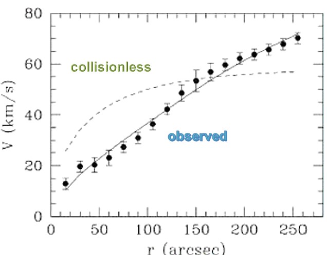
as result of the inferred dark matter halo density profiles, we detect core radii ranging from pc, in the dwarf galaxies, to kpc, in the giant ones Salucci:2018hqu , as shown in Fig. 27. Thus, the sizes of the inner halo regions of constant DM density of different galaxies possess an impressive large range of values, ruling out the case in which all objects have a similar value for the size due to a dark particle-related physical process, as in the case of the (simplest) self-interacting DM scenario.
Within the classic CDM scenario, in which the density cores are obviously absent, the only reasonable core-forming process relies on the feedback mechanism involving supernovae explosions (e.g. Ref. Pontzen:2014lma ; DiCintio:2013qxa ) whose energy, injected in the interstellar gas, although by means of a very indirect and fine tuned process, is able to warm up the inner DM halo and create a constant DM density region. However, the recent evidence of the existence in dwarfs, giant and LSBs galaxies, see Refs. Karukes:2017kne ; DiPaolo:2019eib , all systems for which this mechanism is inefficient due to the insufficient number of SN explosions occurring the unit of time, rules out the CDM + baryonic feedback scenario as a viable explanation for the presence of the DM halo cores in the CDM scenario.
Therefore, in all disk systems, and in many spheroidal systems Salucci:2011ee , the total mass distribution consists in 1) a spherical dark matter halo with two structural parameters: a core radius and a central halo density, both varying among galaxies and 2) a stellar component (disk or spheroid) with two structural parameters: the stellar mass and its photometric radius , also both varying among galaxies.

A further and perhaps more serious issue for the collisionless nature of the dark matter content of the Universe arises from the realization that all the above galaxy structural parameters are found related among themselves, in detail, those of the DM component: , strongly correlate with those of the luminous component, and (see Ref. Salucci:2020eqo and references therein). In order to realize the importance of such evidence let us first remind that: and are the spherical DM density and the luminous surface density. Then, for galaxies and their DM halos, is a quantity deeply inserted in the Dark world, while is a main quantity of the Luminous world. Surprisingly, these two quantities, that, incidentally, are obtained from observations in totally different ways, strongly correlate over three orders of magnitudes, see Fig. 27, giving rise to a tight relationship. The latter is the strongest evidence for a dark matter-luminous matter connection leading us to invoke a direct interaction between the dark particles and the Standard Model particles of the stellar disk/spheroid beyond the collisionless status of the pure gravitational interaction. However, one can claim a full entanglement between the dark and the luminous components of galaxies, evidenced by the existence of Universal Rotation Curve Salucci:2007tm ; Karukes:2017kne ; DiPaolo:2019eib .
Let us stress that such evidence in the dark and luminous mass distribution in galaxies, allied with a complete non-detection of the WIMP particle from accurate astrophysical observations and from properly devised experiments in underground laboratory or at LHC collider (e.g. Ref. Arcadi:2017kky ), has recently opened the way for old and new scenarios in which the DM particles are other than cold and collisionless WIMPS, such as keV fermions, ultra light axions, self-interacting particles, boson condensates and interacting particles (e.g. Refs. Spergel:1999mh ; Hui:2016ltb ; Drewes:2016upu ; Visinelli:2017imh ).
Thus, the dark matter phenomenon at galactic scales seems to provide us with a portal towards the true nature of dark particle that clearly appears to be much more complex than cold, collisionless and particle mass independent as that of the CDM Universe. Regarding this latter, the lack of coldness in the dark particles in galaxies and their emergent capability to sustain interactions with themselves or/and Standard Model particles, are likely to be fatal for its ambition to represent the actual cosmos Salucci:2020eqo .
IX Stepping Up to the New Challenges
Coordinators: Wendy Freedman, Adam Riess, and Arman Shafieloo.
Contributors: Elcio Abdalla, Luis Anchordoqui, Nikki Arendse, Micol Benetti, Emanuele Berti, Kimberly K. Boddy, Alexander Bonilla, Erminia Calabrese, Bozena Czerny, Maria Dainotti, Eleonora Di Valentino, Celia Escamilla-Rivera, Ian Harrison, Dhiraj Kumar Hazra, J. Colin Hill, Daniel Holz, Ryan E. Keeley, Ruth Lazkoz, Benjamin L’Huillier, Matteo Lucca, Roy Maartens, Dinko Milaković, Suvodip Mukherjee, Savvas Nesseris, Rafael Nunes, Antonella Palmese, Leandros Perivolaropoulos, Levon Pogosian, Dan Scolnic, Neelima Sehgal, Joseph Silk, Tommaso Treu, Jian-Min Wang, Amanda Weltman, Radosław Wojtak, Gong-Bo Zhao.
In order to address all the open questions, and to change the CDM from an effective model to a physical model, testing the different predictions, the goals for the next decade will be to:
-
•
improve our understanding of systematic uncertainties;
-
•
maximize the amount of information that can be extracted from the data by considering new analysis frameworks and exploring alternative connections between the different phenomena;
-
•
improve our understanding of the physics on non-linear scales;
-
•
de-standardize some of the CDM assumptions, or carefully label them in the survey analysis pipelines, to pave the road to the beyond-CDM models tests carried out by different groups.
This agenda is largely achievable in the next decade, thanks to a coordinated effort from the side of theory, data analysis, and observation. In 4 separate LoIs DiValentino:2020vhf ; DiValentino:2020zio ; DiValentino:2020vvd ; DiValentino:2020srs , we provide a thorough discussion of these challenging questions, showing also the impossibility we have at the moment of solving all the tensions at the same time.
The next decade will provide a compelling and complementary view of the cosmos through a combination of enhanced statistics, refined analyses afforded by upgraded experiments and next-generation space missions and facilities on Earth:
-
•
Local distance ladder observations will achieve a precision in the measurement of 1% Riess:2020xrj .
-
•
Gravitational time delays will reach a precision on without relying on assumption on the radial mass density profiles Birrer:2020jyr with resolved stellar kinematics measurement from JWST or the next generation large ground based extremely large telescopes (ELTs).
-
•
CMB-S4 will constrain departures from the thermal history of the Universe predicted by the SM Abazajian:2019eic ; Abazajian:2019tiv . The departures are usually conveniently quantified by the contribution of light relics to the effective number of relativistic species in the early Universe, Steigman:1977kc . CMB-S4 will constrain at the 95% confidence level allowing detection of, or constraints on, a wide range of light relic particles even if they are too weakly interacting to be detected by lab-based experiments Abazajian:2019eic . CMB spectral distortions will be another possible avenue to test a variety of different cosmological models in the next decade Chluba:2019kpb ; Kogut:2019vqh ; Lucca:2019rxf
-
•
The Euclid space-based survey mission EUCLID:2011zbd and Dark Energy Spectroscopic Survey (DESI) DESI:2016fyo will use cosmological probes (gravitational lensing, baryon acoustic oscillations (BAO) and galaxy clustering) to investigate the nature of DE, DM, and gravity Capozziello:2011et .
-
•
The Rubin Observatory Legacy Survey of Space and Time (LSST LSST:2008ijt ) is planned to undertake a 10-year survey beginning in 2022. Rubin/LSST will chart 20 billion galaxies, providing multiple simultaneous probes of DE, DM, and CDM LSSTScience:2009jmu ; Zhan:2017uwu ; Sahni:2006pa .
-
•
The Roman Space Telescope (formerly known as WFIRST akeson2019wide ) will be hundreds of times more efficient than the Hubble Space Telescope, investigating DE, cosmic acceleration, exoplanets, cosmic voids.
-
•
The combination of Rubin/LSST, Euclid, and Roman/WFIRST will improve another factor of ten the cosmological parameter bounds, allowing us to distinguish between models candidates to alleviate the tensions.
-
•
The Square Kilometre Array Observatory (SKAO) will be a multi-purpose radio-interferometer, with up to 10 times more sensitivity, and 100 times faster survey capabilities than current radio-interferometers, providing leading edge science involving multiple science disciplines. SKAO will be able to probe DM properties (interactions, velocities and nature) through the detection of the redshifted 21 cm line in neutral hydrogen (HI), during the so-called Dark Ages, before the period of reionization. SKAO will also be able to test the DE properties and the difference between some MG and DE scenarios by detecting the cm HI emission line from around a billion galaxies over 3/4 of the sky, out to a redshift of .
-
•
GW coalescence events will provide a precise measurement of Schutz:1986gp ; LIGOScientific:2017adf ; LIGOScientific:2021aug . With the LIGO-Virgo-KAGRA network of GW detectors, it is expected to constrain to a precision of with about binary neutron star events Chen:2017rfc ; Feeney:2018mkj . Among the sources without electromagnetic counterpart (called dark standard sirens), either by using the statistical host identification technique Gray:2019ksv ; Palmese:2019ehe , or using the spatial cross-correlation Oguri:2016dgk ; Mukherjee:2020hyn ; Bera:2020jhx of the GW sources with spectroscopic galaxies detectable from DESI and SPHEREx Diaz:2021pem , one can achieve a similar precision with a few thousands of dark sirens from the future detector network. The dark siren measurement of the expansion history may also be possible from the mass spectrum of binary black holes by using a few hundreds of sources, if the mass spectrum can be standardized Farr:2019twy ; Mastrogiovanni:2021wsd ; Mukherjee:2021rtw ; Ezquiaga:2022zkx .
-
•
CERN’s LHC experiments ATLAS and CMS will provide complementary information by searching for the elusive DM particle and hyperweak gauge interactions of light relics Buchmueller:2017qhf ; Penning:2017tmb ; CidVidal:2018eel ; Anchordoqui:2020znj . In addition, the ForwArd Search ExpeRiment (FASER) will search for light hyperweakly-interacting particles produced in the LHC’s high-energy collisions in the far-forward region Ariga:2018pin ; Ariga:2019ufm ; Feng:2019bci .
In what follows, we review the cosmological observations and challenges we will face in next coming years.
IX.1 Future Investigations in Cosmology
IX.1.1 Supernova Cosmology
SNe Ia remain the premier tool to link the very local Universe () to the Hubble flow and beyond. Over the next decade, there will be a wealth of data from recently finished and upcoming surveys that will be released. At low- (, the statistics will increase from current samples by a factor of from surveys like ZTF and YSE; at mid-z , statistics will increase by a factor of from Rubin/LSST; and at high- (), statistics will increase by a factor of from the Roman Space Telescope. While the predominant cosmological measurements with SNe Ia have been with the Hubble diagram to measure or or from its role in the distance ladder to measure , the large increase in statistics will enable its usage for a variety of different cosmological measurements. These are described in Ref. Scolnic:2019apa and include measurements of from peculiar velocities at low- (Stahl:2021mat, ) and from the impact of lensing at high- (Zhai:2020axw, ) and further measurements of from lensed SNe Ia LSSTDarkEnergyScience:2019dgr .
There are limitations to how well analyses will be able to leverage this boon in statistics. First, for the direct distance ladder measurement of , current measurements are limited by the number of SNe Ia that have exploded very nearby (), which only occurs roughly once per year. As current measurements utilize now SNe Ia to calibrate the second rung of the distance ladder Riess:2021jrx , it will be difficult to significantly improve this measurement unless measurements of the Cepheids or TRGB can be made accurately at higher distances. Second, as the statistics grow by orders of magnitude, pushing down the systematic floor will become an even higher priority. For measurements of , this means that the sample of SNe used to calibrate Cepheids/TRGB is consistent with the sample of SNe used in the Hubble flow. For measurements of , this means improving calibration, constraints on evolution, etc.
IX.1.2 Local Distance Ladder
The local distance ladder remains the most precise and direct method to produce a high precision determination of the local value of the Hubble constant. There is much reason for optimism for continued progress due to the availability of new facilities like JWST, the Roman and Rubin Observatories, ELTs, and LIGO-Virgo-KAGRA as well as future data releases from Gaia. These facilities are likely to improve upon current measurements while improving the connections between the nearest links. While the distance ladder is approaching the ambitious goal of a 1% determination of the Hubble constant, we may anticipate this goal being approached by a broader range of methods than those available now. Standard Sirens have the potential to provide a fully independent check on the local distance ladder though calibration uncertainties may produce an error floor short of the 1% goal.
IX.1.3 Spectroscopic Galaxy Clustering
The BAO and RSD measurements available in the next decade will provide key information of the expansion and growth history of the Universe, respectively. Compared to the precision offered by existing galaxy surveys such as SDSS BOSS BOSS:2012dmf and eBOSS Dawson:2015wdb , surveys in the next decade, including DESI DESI:2016fyo , PFS PFSTeam:2012fqu , Euclid EUCLID:2011zbd , Roman Spergel:2015sza , Rubin/LSST LSSTScience:2009jmu and so forth, are able to tighten the constraint on both BAO and RSD parameters significantly in a wide range of redshifts, thanks to the order-of-magnitude increase in the optical spectra to be collected.
Challenges exist to reach that precision though, as efforts are needed to mitigate both the theoretical and observational systematics when analyzing the clustering of galaxies. In this regard, the goal for the BAO measurement is relatively more straightforward to achieve, as the BAO signal is more robust against systematics BOSS:2016apd ; Ding:2017gad . The measurement of RSD, however, requires more care to control the impact from both the observational and theoretical systematics. The observational systematics, for example, can root from issues of target selection from the imaging data, the effect of fibre collision, etc (see deMattia:2020fkb for a recent study on the eBOSS ELG sample). Theoretical systematics may include biases for inferring RSD parameters using a fixed template, as commonly used for RSD measurements from existing surveys. Recent development of the EFT-based approach can effectively remove the dependence on the template Baumann:2010tm ; Carrasco:2012cv ; Perko:2016puo ; Blas:2016sfa ; Ivanov:2018gjr , although more nuisance parameters are needed.
It is commonly known that the BAO data, on its own, can only measure the product , where is the sound horizon at the baryon decoupling. However, one can measure both and separately in a way that is independent of the early Universe physics (e.g., physics prior and during recombination) if the BAO data is combined with a prior information on Pogosian:2020ded . One possibility is to combine BAO with the CMB lensing and galaxy lensing data, which provide a handle on with practically no dependence on recombination physics. Alternatively, one could simply do a consistency test by taking the value of determined from CMB anisotropies and using it as a prior in the BAO analysis to see if the deduced values of and agree with those obtained from CMB. Any disagreement would signal a missing ingredient in the model used to determine when analyzing the CMB data. As forecasted in Ref. Pogosian:2020ded , the DESI BAO data, combined with the Planck prior on , will be able to determine to 0.5% accuracy, or .
Over the past five years, full-shape analyses of galaxy clustering datasets have proven their worth as a tool to constrain both the CDM cosmological model and a wealth of extensions (e.g., Ivanov:2019hqk, ; DAmico:2020kxu, ; Chudaykin:2020ghx, ; Ivanov:2020ril, ; Xu:2021rwg, ; DAmico:2022gki, ; Cabass:2022wjy, ; Vagnozzi:2020rcz, ). In the next decade, the power of such tools will only increase as the survey volume grows, and will eventually lead to large scale structure dominating the constraining power on a wide variety of parameters.
Whilst significant improvements will undoubtedly be possible by applying the current analysis methods and pipelines (which have already been tested on simulations larger than the observable Universe (Ivanov:2021kcd, ; Nishimichi:2020tvu, ; Chen:2020fxs, )) to upcoming data (e.g., Chudaykin:2019ock, ), improved theoretical modelling will sharpen the constraints further still. The error on the Hubble parameter measurement from this method will reach with the currently available power spectrum and bispectrum models Chudaykin:2020aoj ; Chudaykin:2020hbf ; Ivanov:2021kcd . However, even better results can be obtained from extending the EFT calculations up to higher-loop order, such as implementation of the two-loop and three-loop power spectra (Carrasco:2013mua, ; Baldauf:2015aha, ; Konstandin:2019bay, ), one-loop bispectrum (Eggemeier:2018qae, ), or two-loop bispectrum (Baldauf:2021zlt, ). This will extend the validity of the models, allowing smaller-scale information to be captured in a robust fashion, marginalizing over all relevant galaxy formation and hydrodynamic effects via symmetry arguments. Similar improvements can be obtained from simulation-based inferences (Kobayashi:2021oud, ; Kobayashi:2020zsw, ), although care will be needed to avoid bias arising from hydrodynamic effects not captured in the modelling. Generalization to additional redshift components, such as the bispectrum multipoles, can also add a tranche of new data, and thereby constraining power (Gualdi:2020ymf, ; Philcox:2021eeh, ).
Another promising avenue is via the inclusion of higher-order statistics, such as the galaxy trispectrum or four-point correlation function and beyond. Initial forecasts suggest that the statistics can yield impressive constraining power on (Gualdi:2021yvq, ), arising due to degeneracy breaking, and recently, the first detections of such quantities have been made (Philcox:2021hbm, ; Gualdi:2022kwz, ). Of course, their use will require the development of rigorous theoretical models (Steele:2021lnz, ) that must be tested on simulations (including systematic effects) before their application to data. -point functions are not the only way to proceed, however: field-level inference provides a promising manner in which to analyze the galaxy survey without compression to summary statistics (Schmidt:2020tao, ; Cabass:2019lqx, ; Schmidt:2020viy, ; Seljak:2017rmr, ), and could lead to strong constraints on parameters such as from a perturbative- or simulation-based framework, once the relevant galactic effects are marginalized over.
Finally, it is important to discuss concerns on the applicability of the standard BAO template fitting method in the future. The fixed template method is currently proven to be biased and to result in loss of information for the galaxy RSD/AP measurements. The galaxy redshift clustering data, however, can be efficiently analyzed by means of the EFT-based full-shape method Ivanov:2019pdj ; DAmico:2019fhj . As far as the BAO measurement is concerned, the dependence on the fiducial template is not so strong, and probably it will not cause a large systematic error even in the era of future galaxy surveys Bernal:2020vbb . However, strictly speaking, it is not clear by default what fiducial cosmology should be used in the BAO template. One option is to fix it by first running the full-shape analysis without the post-reconstructed BAO data. This analysis will already constrain the cosmological parameters very tightly Chudaykin:2019ock . Then the BAO template can be calculated for the best-fit full-shape cosmology. All in all, all these arguments suggest that the BAO method does not require a major modification in order to match the precision of the future datasets.
IX.1.4 Cosmic Microwave Background
Over three decades, with observational campaigns from space, balloons, and ground-based telescopes, the CMB has been the driving force in establishing the standard cosmological model. The most stringent limits on the CDM parameters are obtained from Planck data or a combination of Planck/WMAP and ACT/SPT ground-based experiments. These experiments have accumulated observations in temperature and polarization over many frequencies and extended ranges of angular scales. In particular, with the latest Planck data we have hit the limit of cosmic variance over large and intermediate scales in temperature (Planck CMB temperature power spectrum measurements are cosmic-variance-limited for ). However, much more information can be extracted from improved small-scale temperature measurements and high-accuracy polarization data at all scales, which are the key target of the next decade’s CMB experiments.
From the ground there are several ongoing, planned, and future experiments that will continue to improve CMB temperature and polarization observations. For the topics covered here, the most relevant experiments are those pushing observations over extended and high-resolution scales. These include future releases from the ongoing ACT and SPT experiments, as well as new experiments including the Simons Observatory SimonsObservatory:2018koc , the South Pole Observatory, CMB-S4 CMB-S4:2016ple ; Abazajian:2019eic , and the proposed CMB-HD Sehgal:2019nmk ; Sehgal:2019ewc ; Sehgal:2020yja . The new power spectra from these observatories will constrain with sub-percent precision in the context of CDM (e.g. Ref. SimonsObservatory:2018koc ). Even within more extended models, such as those proposed to resolve the tensions discussed earlier, the statistical power of these upcoming measurements will be sufficient to yield precise constraints and potentially discriminate amongst proposed resolutions, an extremely exciting prospect. In addition, the extracted lensing signal will be revolutionary for constraining the growth of structure with percent level constraints on when correlating CMB lensing with other tracers of the matter distribution.
Anomalies in the present CMB data and tensions between CMB temperature and other cosmological datasets in determining cosmological parameters can be tested with much better precision with upcoming CMB space- and ground-based surveys. Planck temperature data reveals an anomaly in the lensing amplitude. While this lensing anomaly can be resolved with a closed Universe Planck:2018vyg ; DiValentino:2019qzk ; Handley:2019tkm , it aggravates the already existing tensions between the observations in determination of and . Atacama Cosmology Telescope ACT:2020gnv temperature and polarization data, however, do not find this lensing anomaly and the standard model stays consistent with the data. Several new physics candidates and different possibilities of systematic uncertainties have been proposed to solve these discordances. These anomalies and disagreement between CMB datasets and the necessity of new physics will be tested with upcoming observations. Three major improvements in upcoming observations will be able to help in this regard. Firstly temperature anisotropy measurements from ground-based experiments such as Simons Observatory, CMB-S4, and CMB-HD will be able to explore the small differences between Planck and ACT at much better precision. Cosmic-variance-limited polarization measurements from LiteBIRD out to and small-scale polarization data from the ground-based surveys will help in identifying the potential source of anomalies and tensions. Finally, precise measurements of the lensing potential will also independently estimate the lensing amplitude and thereby can provide a statistically significant angle in the study of the lensing anomaly.
The most advanced proposal for a next-generation CMB satellite is the JAXA-led LiteBIRD satellite LiteBIRD:2022cnt .
With a predicted launch towards the end of the decade, LiteBIRD aims to measure the CMB temperature and polarization anisotropies with unprecedented precision and with the ultimate goal to deeply characterize the signal from inflation Snowmass2021:Inflation , ruling in or out well-motivated inflation models. The new maps will help shed light on existing parameter tensions in two ways: 1) LiteBIRD will provide a new, independent of Planck satellite measurement, which will be highly robust to systematic effects due to the use of data from a single, well calibrated CV limited polarization data up to 0.2 degree scales; 2) the new E-mode measurements will provide a new, cosmic-variance-limited measurement of reducing degeneracies with other parameters and in particular.
As already clear from the previous sections, the experimental effort invested in the cosmological landscape has been extremely prolific in the past decades and will continue to grow in the coming years. However, there are some intrinsic limitations in many observables that do not depend on the sensitivity or the duration of the given experiment, and can only be overcome with complementary probes. For instance, in the case of the CMB anisotropies, the presence of the cosmic variance or the well-known degeneracy between and , as well as the limited observable scales, limit the amount of information that can be extracted from these measurements of the last-scattering surface.
In this regard, CMB spectral distortions (SDs) Zeldovich:1969ff ; Sunyaev:1970er ; 1991A&A…246…49B ; Hu:1992dc ; Hu:1993gc ; Hu:1995em ; Chluba:2011hw have been shown to have a remarkably deep synergy with the observation of the CMB power spectra PRISM:2013fvg ; Chluba:2013pya ; Chluba:2019nxa ; Chluba:2019kpb ; Lucca:2019rxf ; Fu:2020wkq ; Schoneberg:2020nyg . In fact, they are mainly produced in the pre-recombination era by any process that affects the energy spectrum of the CMB photons, and are therefore predicted to exist even within the standard CDM model Chluba:2011hw . In this way, they enable to probe a large section of the history of the Universe which overlaps and complements the one already tested by means of the CMB power spectra. The applications in this direction range from CDM Chluba:2016bvg to models invoking BSM physics Chluba:2013wsa , from inflation Schoneberg:2020nyg to recombination Hart:2020voa .
In particular, one of the main production mechanisms within CDM is the dissipation of acoustic waves Chluba:2012gq . This effect takes place when the length scale of the density anisotropies is comparable to the mean free path of the CMB photons, so that the latter stream from the overdense to the underdense regions effectively creating a flow of energy injection which ultimately affects the global energy spectrum. Because of Thompson and Coulomb interactions, the photons end up dragging electrons and protons, which results in an isotropization of the plasma and a damping of the anisotropies at small scales, effect known as Silk damping. Since the amount of density anisotropies at a given scale directly depends on the value of primordial power spectrum (PPS) at that scale, SDs are very sensitive to the cosmological parameters ruling the PPS. This dependence and the fact that SDs are produced prior to recombination are of significant importance as they allow to probe the shape of the PPS (and the inflationary potential more in general) over more than four decades in Fourier space otherwise unexplored by other (complementary) measurements. In combination with, for instance, the CMB observation by Planck this would in principle allow to test the inflationary epoch to an unprecedented degree of precision (see e.g. Ref. Schoneberg:2020nyg ). It is also worth nothing that, as shown in Ref. Hart:2020voa , also the eventual observation of the cosmic recombination radiation Chluba:2015gta would further increase the sensitivity of SDs to inflation, on top of the large amount of information it would provide on the recombination epoch.
Additionally, as recently pointed out in Ref. Lucca:2020fgp , the fact that SDs can put strong constraints on the scalar spectral index can also play a significant role in the Hubble tension, see Sec. IV. Indeed, many extensions of the CDM model recently proposed to address this tension, such as the EDE and the SI models discussed in Secs. VII.4.2 and VII.7.12, respectively, introduce significant shifts in the standard cosmological parameters in the attempt to compensate for the new physics while still accurately fitting the CMB power spectra. This inevitably introduces strong degeneracies between the affected standard parameters and the model-specific quantities. Since one of the most common parameters that vary in these scenarios is , SDs constitute an ideal independent probe to break the aforementioned degeneracies and potentially constrain the efficacy of these models as solutions to the Hubble tension. Moreover, in the context of the Hubble tension, SDs have also been advanced as a possible avenue to obtain an (almost) model-independent measurement of the value Abitbol:2019ewx . This can be achieved by precisely observing the evolution of the CMB monopole temperature over an extended timescale, thereby obtaining a measure for the cooling of the Universe and thus its expansion rate.
Interestingly, together with the dissipation of acoustic waves, SDs are also sensitive to the dissipation of tensor modes, making them a window to another large class of inflationary scenarios Chluba:2014qia . In this context, as recently discussed in Ref. Kite:2020uix , through this mechanism SDs are also able to probe primordial GWs over six orders of magnitude in frequency space. This can tightly bound a variety of scenarios involving phase transitions or cosmic strings Kite:2020uix , among many more.
Along with the spectral distortions on the CMB monopole, spatially fluctuating polarised CMB spectral distortion can also arise due to conversion of photons to axions (or axion like particles (ALPs)) in the presence of external magnetic field as proposed in Refs. Mukherjee:2018oeb ; Mukherjee:2019dsu . The measurement of the polarised axion distortion will provide a new way to detect the coupling of photons with ALPs in the mass range –eV. This is possible from the upcoming ground based CMB experiment such as Simons Observatory, CMB-S4, CMB-HD and from space-based CMB telescope LiteBIRD.
The complementary between CMB anisotropies and SDs mentioned at the beginning of this section can also be applied to models requiring, for example, primordial magnetic fields (PMFs) Jedamzik:1999bm ; Kunze:2013uja ; Jedamzik:2018itu , DM with non-standard characteristics, such as decays Hu:1993gc ; Lucca:2019rxf or interactions Ali-Haimoud:2015pwa ; Slatyer:2018aqg , Axion-Like Particles Mukherjee:2018oeb ; Mukherjee:2019dsu and dark photons, or primordial black holes Tashiro:2008sf ; Lucca:2019rxf ; Acharya:2020jbv ; Eroshenko:2021oeq ; Papanikolaou:2021uhe . Many of this scenarios have also been shown to solve either the Hubble tension, such as for PMFs Jedamzik:2020krr , the EDGES anomaly, such as for DM-b interactions Kovetz:2018zan , or the tension, such as for DM-photon interactions Stadler:2018jin ; Becker:2020hzj . Therefore, also in this context SDs could play a competitive and complementary role in the search for a solution to these modern problems.
However, profiting from the constraining power of SDs will only be possible with the advent of advanced dedicated missions such as SuperPIXIE Kogut:2019vqh and Voyage 2050 initiative Chluba:2019nxa , which, most likely, will have to be preceded by pathfinders from the ground or space. Therefore, the goal of the next decade in the context on CMB SDs will not only have to be in the theoretical and numerical development of the field, but will also have to be particularly devoted to the experimental realization of a concrete observational strategy to measure both temperature anisotropy and spectral distortions in a same setup Mukherjee:2018fxd ; Mukherjee:2019pcq .
IX.1.5 Weak Lensing
A number of ongoing and planned weak lensing surveys promise to provide significantly tighter constraints on the amplitude of matter fluctuations and the equation of state of dark energy (see Tables 3 and 4).
These include ongoing surveys such as Kilo-Degree Survey (KiDS) KIDSws , Dark Energy Survey (DES) DESws , Hyper Suprime-Cam (HSC) HSCws , and planned to start surveys such as the Rubin Legacy Survey of Space and Time LSSTws , Euclid Euclidws , Nancy Grace Roman Space Telescope NGRSTws , and the The Ultraviolet Near- Infrared Optical Northern Survey (UNIONS) which is a collaboration between two the Hawai’ian observatories CFHT (Canada-France-Hawaii Telescope on Mauna Kea) and Pan-STARRS (Panoramic Survey Telescope and Rapid Response System on Maui) UNIONS ; CFISws ; Pan-STARRSws .
These lensing surveys promise not only to map the photo-z sky and dark matter but also constrain the growth of large structures to unprecedented accuracy and precision.
IX.1.6 Time Lag Cosmography and Time Delay Cosmography
In this Section we describe two methods based on ”standard clock”, i.e. the measurement of time intervals that can be converted into a cosmic distance and thus a cosmological tool. First, we describe the use of the time lag between variability of the accretion disk surrounding black holes, which we refer to as ”time lag cosmography”. Then we describe the use of the time delay between multiple images of strongly gravitationally lensed sources, which we refer to as ”time delay cosmography” (Treu:2016ljm, ).
Measurements from Quasars with Rubin/LSST Monitoring.
The oldest method to use active galactic nuclei for cosmology is the method based on continuum time lag measurements Collier:1998ev in the accretion disk. The method is conceptually simple, it is based on the concept of accretion disk model of Ref. Shakura:1972te , which well describes the accretion disk at radii of order of 100 - 1000 gravitational radii, where the optical continuum forms. The method is not very sensitive to the innermost part of the accretion flow, close to the black hole, see e.g. Ref. (Kammoun:2020pno, ), where the local approximation of the disk emission by a black body might not apply (Czerny:2003hj, ; Kubota:2018cuj, ). However, the method was not successful so far since the so called disk size problem appeared: although the time measured delay scaled with the wavelength as expected (, Ref. Collier:1998ev ), the normalization of this relation did not follow the theoretical expectations, and the measured time delays were frequently longer implying larger disk size, see e.g. Refs. Collier:1998ev ; Cackett:2007kw ; Shappee:2013mna ; 2016ApJ…821…56F ; Jiang:2016jua ; DES:2017vao ; 2020ApJS..246…16Y ; 2021arXiv211107385F , although part of the effect may be due to pre-selecting at the basis of S/N requirements and large intrinsic dispersion due to orientation, spin or accretion efficiency (Homayuni2019, ). Disk sizes larger than expected were also found from microlensing measurements, see e.g. Ref. (Rauch1991, ). The problems might have come from the considerable departure from the local black body emission, see e.g. Ref. (Hall:2017hnc, ), but recent dense reverberation mapping proved that the problems with disk size come from the contribution to the continuum from the Broad Line Region, most notably Balmer continuum, but also Fe II continuum (Cackett:2017htp, ; Edelson:2018gbe, ; 2022MNRAS.509.2637N, ). Identification of the problem opens a way to use the multicolor monitoring data from Rubin/LSST from the Dip Drilling Fields to cosmology (2020ApJS..246…16Y, ), if the corrections due to Balmer continuum and Fe II are implemented. It will nicely complement the quasar method based on emission line time delays which allow to constrain other cosmological parameters, see e.g. Refs. (2021ApJ…912…10Z, ; Khadka:2021ukv, ) but is not yet applicable to measuring since it still requires external scaling.
Constraining Cosmology with Multiply Imaged Supernovae and Quasars.
Time delay cosmography relies on the gravitational time delay between multiple images of a lensed variable source to constrain cosmology. The time delays between the images are primarily sensitive to the Hubble constant, but also weakly to several other cosmological parameters such as the matter density, curvature of the Universe and the EoS parameter for dark energy and its evolution over time. Other aspects that influence the time delays are the lens potential, microlensing due to substructure in the lens galaxy, and line-of sight-structures. If accounted for these effects properly, gravitationally lensed quasars and supernovae (glSNe) can be powerful probes to yield constraints on cosmological parameters, independently from the distance ladder or CMB.
Multiply imaged quasars have been used for cosmology since their discovery in the late 70s. Since the year 2000 advances in sample size, data quality and analysis methods have shown that they can be used to determine the Hubble constant with high precision and accuracy. An account of the history of quasar based time delay cosmography and future prospects can be found in the review by Treu and Marshall Treu:2016ljm . Briefly, hundreds of multiply imaged quasars have already been discovered and future surveys by the Euclid, Roman, Rubin, and SKAO Telescopes are going to increase the samples by orders of magnitudes (e.g. Oguri:2010ns, ). The precision and accuracy of the inferred cosmology will not be limited by sample size, but rather by the quality of the follow-up data and understanding of systematic errors, which are in many case common to the study of glSNe, and therefore are discussed below.
When Refsdal predicted in 1964 how the phenomena of strong gravitational lensing could be used to calculate the cosmic expansion rate Refsdal1964 , he initially suggested glSNe for this purpose. Only recently has this avenue become a reality. The first discovery of a glSN was made by the Panoramic Survey Telescope and Rapid Response System 1 (Pan-STARRS1), when it detected an unusually red and bright SN. After spectroscopic confirmation of a foreground lensing galaxy, the transient was classified as a gravitationally lensed SNIa, although the imaging data had insufficient resolution to separate the images XXX:2014xxi . The Hubble Space Telescope (HST) provided data of the first resolved and multiply-lensed SN, a core-collapse SN appropriately named ”Refsdal” Kelly:2014mwa . Four images were detected around an elliptical galaxy, and the prediction that another one would appear in a second host-galaxy image was verified one year later Kelly:2015xvu . SN Refsdal alone will provide a measurement of with a statistical error of 7 Grillo:2018ume .
The intermediate Palomar Transient Factory (iPTF) identified glSN iPTF16geu, which was followed up by ESO VLT, Keck Observatory, and HST and spectroscopically identified as a type Ia SN Goobar:2016uuf ; Cano:2017rhv . The third resolved strongly lensed supernova AT2016jka (”SN Requiem”) was discovered in Hubble Space Telescope data, and is predicted to host a fourth image in two decades time, which should allow for a sub-per cent precision measurement of the time delay Rodney:2021keu .
Current transient surveys capable of detecting glSNe, such as the Zwicky Transient Facility (ZTF) and Pan-STARRS, are only estimated to discover a few objects a year (6-9 Goldstein:2016fez ; Goldstein:2018bue ; Wojtak:2019hsc and two Wojtak:2019hsc for ZTF and Pan-STARRS, respectively). The true potential of discovering and observing glSNe will be unveiled by future telescopes, which are predicted to discover orders of magnitude more. The Rubin Observatory Legacy Survey of Space and Time (LSST) LSSTScience:2009jmu is estimated to detect around 89 type Ia and 250 core collapse glSNe a year Goldstein:2016fez ; Goldstein:2018bue ; Wojtak:2019hsc , although the actual discovery rates may be lower when employing more restrictive criteria for selecting plausible candidates. The discovery rates of the Roman Space Telescope Green:2012mj , estimated with the image multiplicity method, are 9-56 Ias and 17-126 core collapse SNe a year, depending on the observing strategy Pierel:2020tav . The majority of the lensed core collapse SNe will be type IIn; however, this prediction is based on a relatively poor set of observed spectral templates of type IIn SNe and thus will likely be a subject to further improvement in the future. Gravitationally lensed SNe appear as peculiarly bright (relative to type Ia brightness at redshift of the apparent host galaxy) and multiply imaged sources. These are the two main observational properties which can be used to select plausible glSN candidates. Novel techniques can be employed to help identify glSNe with partially blended images, such as neural networks trained on time series of images (Ramanah:2021bpb, ; Morgan:2021oxb, ). Another strategy for finding glSNe is to monitor known lensed galaxies (Craig:2021vld, ). Precise measurements of gravitational time delays will strongly rely on follow-up observations compensating insufficient cadence of large transient surveys LSSTDarkEnergyScience:2019dgr .
Gravitationally lensed quasars and supernovae are highly complementary. In the remainder of this section we compare the pros and cons of each variable source and conclude by highlighting the common challenges. Firstly, lensed quasars are around 60 times more numerous than lensed supernovae Oguri:2010ns . In terms of the variability, supernovae (especially type Ia) have well-described light curves that can be fit with established templates, while quasars are characterized by a stochastic variability. Another important difference between glSNe and lensed quasars is that supernovae fade away over time. This poses a challenge, since follow-up observations are highly time-sensitive, but it also offers an advantage, as it allows for better kinematic follow-up observations of the lens and host galaxy once the supernova has faded away (Ding:2021bxs, ). Such velocity dispersion measurements can help constrain the mass sheet degeneracy, which is a transformation of the potential that leaves all imaging observables the same, while changing the time delays 1985ApJ…289L…1F ; 1988ApJ…327..693G ; Saha:2000kn . Type Ia supernovae offer another way of breaking the mass sheet degeneracy: their standard candle nature can provide an estimate of the absolute magnification Foxley-Marrable:2018dzu ; Birrer:2021use . However, it is worth noting that these constraints depend on the precision of type Ia SN standardisation, as current samples still yield intrinsic scatter in the Hubble diagram of around 0.12 mag (or 6 % in distance) Pan-STARRS1:2017jku . The utility of the standard candle nature of lensed type Ia SNe can also be limited by the effect of microlensing, which gives rise to extra stochastic magnifications in every lens image Yahalomi:2017ihe . Another difference is that glSNe typically have a smaller angular size and smaller image separations than lensed quasars, due to the lower mean redshifts of glSNe. Therefore, lensed SNe are prone to have very short time delays, of the order of several days or weeks. This means that time-delay measurements only require weeks of follow-up observations instead of year-long monitoring campaigns as is usual for lensed quasars. However, obtaining precise measurements of such short time delays can be highly challenging. The small angular size of glSNe also leads to a higher sensitivity to microlensing from stars and other substructures in the lens galaxy. Microlensing can perturb light curves independently in each supernova image, which can lead to additional systematic errors in time delays of order 4 Goldstein:2017bny . Fortunately, effects of microlensing can be minimised if multi-colour follow-up observations are obtained of the initial phase of the explosion. In this phase, the SN can be approximated as a point source and thus look identical in every filter, which leads to the same microlensing distortion across all wavelengths. This ”achromatic” phase is expected to last until 3 rest-frame weeks after the explosion Goldstein:2017bny ; LSSTDarkEnergyScience:2019dgr , in which 70 of Rubin/LSST glSN Ia images will be discovered. The useful implications are that the microlensing effects are expected to cancel out in early time colour curves, reducing the systematic uncertainties to 1 for typical Rubin/LSST systems Goldstein:2017bny . Since microlensing is capable of altering the brightness of the multiple images, thereby changing whether they fall above or below our detection limits, it could impact the number of glSNe and lensed quasar we will be able to observe.
For both types of variable sources, the precision and accuracy of the inferred cosmology will likely not be limited by sample size but by the quality of follow-up data and systematic uncertainties associated with the analysis. Most of these are common between lensed quasars and supernovae. In addition to the time delays themselves, that will likely required dedicating monitoring capabilities to supplement the cadence of the survey themselves, e.g. through a dedicated 3-4m class telescope, the cosmological inference requires: i) angular resolution images at resolution of 10mas or better; ii) spatially resolved kinematics of the deflector galaxy or cluster galaxies to break the mass sheet degeneracy and the mass anisotropy degeneracy Birrer:2020tax ; Xu:2011ru ; iii) information about the structure along the line of sight. Whereas the information about the mass along the line of sight will likely be provided by the same surveys used for the discovery of the targets, in combination with high precision next generation cosmological simulations, the high angular resolution imaging and spatially resolved kinematics can only be obtained with the James Webb Space Telescope or the next generation of extremely large telescopes.
With proper follow-up, time delay cosmography will be able to deliver measurements of the Hubble constant with a precision and accuracy of 1%, independent of all other methods, contributing to the resolution of the Hubble tension (e.g., Birrer:2020jyr, ).
IX.1.7 Gravitational Wave Cosmology
It took almost 100 years for the prediction of gravitational waves to finally be directly confirmed LIGOScientific:2016aoc . Since the first detection of gravitational waves in 2015 by LIGO-Virgo Scientific Collaboration LIGOScientific:2016aoc , 90 events from compact object binary mergers have now been observed by the network of LIGO-Virgo detectors LIGOScientific:2021djp , and the field of GW astronomy is exploding.
The third generation ground-based interferometers (such as Cosmic Explorer Reitze:2019iox ; Evans:2021gyd , Einstein Telescope Maggiore:2019uih ) as well as space based gravitational wave detectors (e.g. LISA LISA:2017pwj , TianQin Luo:2015ght , Taiji Hu:2017mde , and DECIGO Kawamura:2020pcg ), scheduled for the next decade, will open an even broader spectrum of gravitational-wave sources, providing novel cosmological probes with great precision. Also, possibly operating in conjunction, these experiments can improve our ability to investigate fundamental physics with GWs. In what follows, some perspectives on GWs for cosmology are presented.
In the next decade, gravitational wave standard sirens (GWSS) Schutz:1986gp ; Holz:2005df ; Dalal:2006qt ; Chen:2017rfc ; DiValentino:2018jbh ; Vitale:2018wlg ; Palmese:2019ehe , the GW analog of astronomical standard candles, are expected to play an important role in the context of cosmology. The amplitude of GWs is inversely related to the luminosity distance from the source, hence they can be used in conjunction with redshift information to the source to probe the distance-redshift relation. Observations of the merger of the binary neutron-star system GW170817, along with the redshift from its host galaxy, identified thanks to the observation of an electromagnetic counterpart, yield at 68% CL LIGOScientific:2017adf . Though this constraint is broad, it does not require any cosmic ”distance ladder” and is model-independent: the absolute luminosity distance is directly calibrated by the theory of general relativity Schutz:1986gp . In other words, GWSS of this kind are an ideal independent probe to weigh in on the Hubble tension problem. Around 50 additional observations of GWSS with electromagnetic counterparts are needed to discriminate between Planck and R19 measurements of with a precision of – Nissanke:2013fka ; Chen:2017rfc ; Mortlock:2018azx . Measurements of this kind can also play an important role in an extended parameter space DiValentino:2017clw ; DiValentino:2018jbh in which CMB data are unable to strongly constrain , in a way that breaks degeneracies amongst parameters. Standard sirens with EM counterparts are therefore expected to be extremely powerful cosmological probes, while the upgrades to the LIGO-Virgo second generation design sensitivities are critical to provide the above desired number of BNS merger detections.393939Cosmic Explorer and Einstein Telescope are expected to observe far more binary neutron star mergers. On the other hand, kilonovae associated with BNS mergers are expected to be close to isotropic, and are thus the most promising of all BNS EM counterparts. However, the kilonova associated with GW170817 was intrinsically faint, and nonetheless was thought to be on the bright end of the kilonova luminosity function. In order to provide new associations, and hence a standard siren measurement that is informative for the Hubble tension, deep optical-to-near-infrared observations will be required to identify the fainter kilonovae, with more precise GW localizations playing a significant role in the success of these follow-up campaigns. Multi-object spectroscopic observations could play a central role in these campaigns through rapid classification of all the viable variable objects in the GW localization regions, which is currently a bottleneck for the identification of counterparts from imaging observations. Experiments such as DESI-II Dawson:2020 could design a specific program aimed at standard siren cosmology through the identification of counterparts and observation of transients host galaxies’ redshifts, along with other key science projects.
Complementary dark GWSS (GW sources without EM counterparts) such as those used in Ref. LIGOScientific:2018gmd ; DES:2020nay ; LIGOScientific:2021aug ; Palmese:2019ehe are expected to provide percent-level uncertainty on after combining a few hundreds to thousands of events from the statistical host identification technique Gray:2019ksv or by identifying the host galaxy for the nearby sources Borhanian:2020vyr using upgraded detector network in the future. In this case, a galaxy catalog overlapping with the GW events is necessary to provide the redshift information of the potential host galaxies. The implementation of this method depends on the completeness of the galaxy catalog up to high redshift, understanding the GW sources population, and better sky localization error of the GW sources. In order to avoid any biased measurement of the Hubble constant Trott:2021fnx , a promising approach can be to use the statistical host identification technique as demonstrated by LIGOScientific:2018gmd ; Gray:2019ksv ; Palmese:2019ehe ; DES:2020nay ; LIGOScientific:2021aug . Another promising method to infer cosmological parameters from dark GWSS consists in cross-correlating GW sources with photometric or spectroscopic galaxy surveys to infer the clustering redshift of the GW sources Oguri:2016dgk ; Mukherjee:2018ebj ; Scelfo:2018sny ; Mukherjee:2019wcg ; Mukherjee:2020hyn ; Bera:2020jhx ; Scelfo:2020jyw ; Diaz:2021pem ; Mukherjee:2022afz . The cross-correlation technique is a promising avenue to achieve a measurement of the Hubble constant from the LIGO-Virgo-KAGRA network operational in its design sensitivity in synergy with galaxy surveys such as SPHEREx and DESI Diaz:2021pem after combining a few hundreds of well-localised GW sources. Moreover, this technique will also make it possible to measure the DE EoS and the connection between GW sources and dark matter from dark standard sirens. Though the implementation of the cross-correlation does not require the host galaxy of the GW source to be present in the catalog, its success will depend on the availability of GW sources with better sky localization error. This may be feasible by using multiple detectors, overlapping galaxy surveys with accurate redshift estimation, and marginalization over the redshift-dependent GW bias parameters Mukherjee:2020hyn ; Diaz:2021pem ; Mukherjee:2022afz . It follows that for the success of dark GWSS appropriate full sky galaxy catalogs that cover the redshift range of GW sources are required. Alternatively, it is possible to use features in the mass spectrum of binary black holes to infer redshift, providing a powerful and independent standard siren probe of cosmology Chernoff:1993th ; Farr:2019twy ; Ezquiaga:2020tns ; Mukherjee:2021rtw ; LIGOScientific:2021aug ; Ezquiaga:2022zkx . These ”spectral sirens” may provide percent-level constraints on the expansion history at and beyond. However, for this technique to work, the mass distribution of the GW sources need to be standardised. Any redshift evolution Mukherjee:2021rtw of the GW mass distribution needs to be mitigated in order to avoid any systematic error in the inference of the cosmological parameters. Another dark siren approach is to use knowledge of the EoS of neutron stars to infer redshift. For third-generation detectors, this would allow us to use these systems as standard sirens to constrain cosmology even in the absence of an electromagnetic counterpart Messenger:2011gi ; Chatterjee:2021xrm . Space-based, low-frequency GW detectors such as LISA may observe well-localized GW signals from SMBH binary mergers with EM counterparts. Depending on uncertainties in SMBH formation models and EM emission mechanisms, these SMBH standard sirens could provide useful constraints on the Hubble constant, and up to Tamanini:2016zlh .
Since standard sirens can be detected at cosmological redshifts, they can be sensitive to other cosmological parameters besides such as and . As would be the case for any other probe, should one assume a specific model that were not true (e.g. CDM), then the inferred parameters from that assumed model would be biased relative to the true ones. In the case of cosmological standard sirens that extend to the bias on the inferred cosmological parameters exceeds when the true model was a Chevallier - Polarski - Linder parameterization (CPL) Chevallier:2000qy ; Linder:2002et model that is consistent with current SN constraints Shafieloo:2018qnc . The biases that arise from assuming the wrong model can be mitigated, however, with the use of model-independent statistics such as Gaussian process regression Keeley:2019hmw . Because of their high redshifts, some GW sources are expected to be strongly lensed Wang:1996as ; Oguri:2018muv ; Li:2018prc ; a catalog of multiply-imaged sources, and associated lensing rates, time-delays, and magnification distributions, may provide additional cosmological constraints Oguri:2018muv ; Xu:2021bfn .
In the next decade, GWSS are expected to provide strong constraints on dark energy, modified gravity, dark matter and neutrinos, and shed light on several other important aspects in cosmology Cai:2016sby ; Pardo:2018ipy ; Du:2018tia ; Yang:2019bpr ; Wei:2018cov ; Zhang:2018byx ; Wang:2018lun ; Zhang:2019ple ; Qi:2019spg ; Yang:2019vni ; Fu:2019oll ; Yang:2020wby ; Bonilla:2019mbm ; Chen:2020zoq .
The physical degrees of freedom of GWs are imprints of the nature of gravity, and by modifying general relativity (GR), we have two major possibilities that can modify and leave fingerprint in the GW signal.
-
•
Propagation Effects: A common feature in almost all gravity theories beyond GR, considering the Universe on large scales, is that the new degrees of freedom in each theory modify the gravitational force/interaction on cosmological scales, mainly to explain the late-time acceleration of the Universe (dark-energy-dominated era). This roughly corresponds to an effective time-varying gravitational constant that will affect the propagation of GWs along the cosmic expansion, which in turn can induce amplitude and phase corrections on the GW signal over cosmological volumes Cai:2016sby ; Pardo:2018ipy ; Du:2018tia ; Yang:2019bpr ; Wei:2018cov ; Zhang:2018byx ; Wang:2018lun ; Zhang:2019ple ; Qi:2019spg ; Yang:2019vni ; Fu:2019oll ; Yang:2020wby ; Bonilla:2019mbm ; Cutler:2009qv ; Nishizawa:2009jh ; Nishizawa:2010xx ; Yagi:2013du ; Nunes:2018zot ; Cai:2017aea ; Saltas:2014dha ; Nishizawa:2017nef ; Belgacem:2017ihm ; Belgacem:2018lbp ; Arai:2017hxj ; Belgacem:2019pkk ; Lagos:2019kds ; Nunes:2019bjq ; Nunes:2018evm ; Belgacem:2019lwx ; DAgostino:2019hvh ; Gao:2019liu ; Belgacem:2019tbw ; Calcagni:2019ngc ; Dalang:2019rke ; Wolf:2019hun ; Nunes:2020rmr ; Baker:2020apq ; Mitra:2020vzq ; Mastrogiovanni:2020mvm ; Mukherjee:2020mha ; Heisenberg:2022lob ; Heisenberg:2022gqk ; Lee:2022cyh . The effective time variation of the gravitational constant could be measured with a few percent precision using a multi-messenger Engel:2022yig approach exploiting the unique relation between the GW luminosity distance, BAO angular scale and the sound horizon at decoupling Mukherjee:2020mha . We may also be able to test the propagation effect from gravitational lensing of GW sources Holz:1997ic ; Mukherjee:2019wcg ; Mukherjee:2019wfw ; Ezquiaga:2020dao ; Ezquiaga:2021ler ; Finke:2021znb , which will provide new tests of general relativity Bettoni:2016mij ; Brax:2017hxh ; Belgacem:2017ihm ; Bonilla:2019mbm .
-
•
Generation Mechanism: By changing the gravity interaction in the inspiral-merger-ringdown phases, we also change the generation mechanism of the gravitational radiation emitted by the binary systems. Such methodology can be quantified through the parameterized post-Einsteinian framework Yunes:2009ke ; Cornish:2011ys ; Carson:2019fxr ; Carson:2019kkh . Future ground-based and LISA observations can lead to improvements of 2-4 orders of magnitude with respect to present constraints, while multiband observations can yield improvements of 1-6 orders of magnitude Perkins:2020tra .
An interesting and realistic approach might be to combine both effects on the waveform signal modeling. Some specific theoretical cases of these effects were recently investigated using the LIGO-Virgo-KAGRA GW Transient Catalog LIGOScientific:2018mvr ; LIGOScientific:2020ibl . On the other hand, searching for polarization modes beyond the GR prediction provides a strong test of GR. This aspect can also be combined with the above mentioned effects. At a local level, the GW information from isolated or binary systems in the strong space-time curvature regime also provides several tests of GR Berti:2015itd . The improvement in amplitude of the spectral noise density in future detectors will be fundamental to investigate the limits of these theoretical aspects.
Another interesting possibility is the detection of stochastic gravitational waves. Direct evidence of GWs has thus far been in the form of coherent measurements of resolved waveforms in processing the detected signals, which can be traced back to their origin as single points. Consequently, only a tiny fraction of these GW can be seen from a presumably much larger population spread throughout space at different scales. The extensive set of unresolved signals corresponding to multiple point sources or extended sources increases incoherently, leading to gravitational-wave backgrounds (GWBs). A variety of different backgrounds is expected, given the range of diverse GW sources in the Universe. Most of these backgrounds are treated as stochastic, as they may be described by a non-deterministic strain signal and are hence referred to as stochastic gravitational-wave backgrounds (SGWBs). Indeed, the existence of a SGWB is a robust prediction of several well-motivated cosmological and astrophysical scenarios operating at both the early and late Universe Maggiore:1999vm ; Caprini:2018mtu ; Giovannini:2019oii . Below we present some of the most prominent observational projects to detect the SGWB across a broad range of frequencies of the GW spectrum.
-
•
Very low frequencies. Cosmic inflation is currently the leading paradigm to explain the initial conditions of our Universe. Single-field slow roll inflation, as well as alternative treatments Benetti:2021uea ; Myrzakulov:2015qaa ; Odintsov:2021kup ; Cannone:2014uqa ; Graef:2015ova ; Ricciardone:2016lym ; Graef:2017cfy ; Baldi:2005gk ; Dimastrogiovanni:2016fuu ; Obata:2016oym ; Cook:2011hg ; Mukohyama:2014gba ; Cai:2016ldn ; Cai:2020ovp ; Stewart:2007fu ; Brandenberger:2014faa ; Hipolito-Ricaldi:2016kqq ; Kinney:2018nny ; Odintsov:2020sqy ; Odintsov:2020zkl ; Trivedi:2020wxf ; Oikonomou:2020oex , predict the existence of a SGWB. Such GWs induce a B-mode pattern in the polarization of the CMB. From the lack of a detection of primordial B-modes, CMB observations place upper limits on the amplitude of the primordial GW power spectrum BICEP2:2018kqh ; Planck:2018vyg . For an angular resolution scale of , these limits can be translated into limits on the amplitude of the SGWB for frequencies Hz. Current ground-based CMB experiments—ACT ACT:2020gnv , BICEP/Keck BICEP2:2018kqh , CLASS Harrington:2016jrz , POLARBEAR/Simons Array POLARBEAR:2015ixw , SPT SPT:2019nip —measure the CMB polarization to high precision and will continue to better constrain primordial B-modes. Upcoming experiments, like Simons Observatory SimonsObservatory:2018koc and CMB-S4 Abazajian:2019eic ; CMB-S4:2020lpa , will achieve even greater sensitivity. In addition, satellite missions such as LiteBIRD LiteBIRD:2022cnt and balloon missions such as SPIDER SPIDER:2017xxz will complement ground-based efforts.404040See Ref. Caldwell:2022qsj for a study of the potential of using an early Universe GW signal to probe fundamental physics.
-
•
Low frequencies. The high-precision timing of Galactic millisecond pulsars enables a search for nHz GWs, which are expected to be generated primarily by SMBH binaries. A GW transiting through the line of sight between Earth and the pulsar distorts the intervening spacetime, altering the expected time of arrival of pulses. A SGWB affects the timing of all pulsars in the Galaxy, causing spatially correlated time-delay signals between pulsar pairs, known as Hellings-Downs correlations Hellings:1983fr . These correlations are primarily quadrupolar, with subdominant contributions from higher multipoles, and are distinct from two main sources of spatially-correlated noise, errors in the terrestrial time standard (monopolar) and errors in the planetary ephemeris (dipolar) 1978SvA….22…36S ; Detweiler:1979wn ; 1990ApJ…361..300F ; Brazier:2019mmu ; NANOGrav:2020gpb . World-wide efforts to search for a SGWB are underway: the North American Nanohertz Observatory for Gravitational Waves (NANOGrav) NANOGrav:2020bcs , the Parkes Pulsar Timing Array (PPTA) Hobbs:2013aka ; Kerr:2020qdo , the European Pulsar Timing Array (EPTA) Desvignes:2016yex , and the Indian Pulsar Timing Array Project (InPTA) Joshi:2018ogr , all operate both individually and as a collective under the International Pulsar Timing Array (IPTA) Perera:2019sca . Recent evidence of a common-spectrum process has provided intriguing hints that a detection may be soon to come, but observing the Hellings-Downs spatial correlation will be key to interpreting any signal as a possible SGWB detection NANOGrav:2020bcs ; Goncharov:2021oub ; Chen:2021rqp .
Distortions of spacetime affect not only the timing of pulsars, but also induce a shift in the apparent position of stars. These shifts may be observed in astrometric surveys Braginsky:1989pv ; Kaiser:1996wk for GWs in the frequency range . Similar to PTAs, the shifts also exhibit particular angular correlations from a SGWB Book:2010pf . Indeed, there are expected cross correlations between PTAs and astrometric shifts that could permit complementary studies Mihaylov:2018uqm ; Qin:2018yhy ; Mihaylov:2019lft ; Qin:2020hfy . Astrometric data from GAIA and extragalactic radio sources have set constraints on the energy density of the SGWB Darling:2018hmc . Future missions such as Theia could provide improved sensitivity Theia:2017xtk .
-
•
Intermediate frequencies. The GWs are emitted mainly by individual binary systems, like, for instance, from binary black holes (BBH), binary neutron stars (BNS), and binary black hole-neutron stars (BBH-NS). The superposition of the signal from these sources over cosmological volumes is expected to form an SGWB of astrophysical origin. This signal strongly depends on the sources that produce them, and we expect that signal to exist in the most diverse frequencies (in this case, for example ) Zhu:2012xw ; Mingarelli:2019mvk ; Jenkins:2018uac . Nevertheless, this specific type of signal has not been detected until the present moment, and only some upper limits on the SGWB signal have been obtained, for instance, the LIGO-VIRGO-KAGRA collaboration reported an astrophysical background with amplitude LIGOScientific:2019vic . With the improvements in instrumental sensitivity in the coming years and the prospects of future detectors like the Einstein Telescope (ET) Maggiore:2019uih , Cosmic Explorer (CE) Reitze:2019iox , and LISA LISA:2017pwj ; Caprini:2019pxz , it is expected to achieve enough sensitivity to detect SGWBs of astrophysical origin.
-
•
Ultra-high frequencies. Recently, IPTA gave hints of GWs from cosmic strings Antoniadis:2022pcn , which has further encouraged the community to build a strong case for experiments that can tackle ultra-high-frequency gravitational waves (UHGW). This is because, on the one hand, cosmic strings are a great scenario that can be analyzed in the multiband frequency range and hence with experiments already covering the low, medium, and high-frequency range (e.g., PTA experiments, LISA and LIGO-Virgo-KAGRA, respectively). Further experiments that can cover the MHz to GHz region are missing. Their construction could then complement the study of cosmic string signals in the broadband frequency range. On the other hand, SGWB due to cosmic origin, for example, from inflation models, from the evaporation of primordial black holes or phase transitions generated when Grand Unified Theories break into the SM or other subgroup can have signals in the MHz to GHz range. Hence, the current GW experiments will not be able to detect them. Different initiatives are being carried out to promote the creation of a network of researchers to develop the science of GW’s in the frequency range above kHz.414141Go to this home page, for example: http://www.ctc.cam.ac.uk/activities/UHF-GW.php
Finally, several authors have pointed to the implementation of GW standard sirens and GW stochastic backgrounds to explore the late and early Universe, in a broad spectrum of possibilities ranging from the Hubble tension Li:2021htg through the search for modified gravity Nunes:2020rmr ; Allahyari:2021enz , variation of the speed of propagation of GWs Bonilla:2019mbm , inflation models Li:2021htg and even explore the exotic fundamental physical possibility as the variation of fundamental constants Nunes:2016plz ; Colaco:2022aut .
IX.1.8 21 cm Cosmology
Up to now, the key probes of large-scale structure in the Universe have been based on galaxy surveys, and the upcoming generation of these surveys promises to deliver a revolutionary advance in precision cosmology. Next-generation galaxy surveys will be complemented by a new type of survey, which will map the 21 cm emission line of neutral hydrogen (HI) in the post-reionization era (). The 21 cm emission of galaxies that contain HI provides a tracer of the dark matter distribution, with extremely precise redshift measurement as a direct by-product of detection. However, the faintness of the emission means that next-generation HI galaxy surveys with SKAO-MID will not be competitive with contemporaneous spectroscopic surveys in the optical/ infra-red bands, although they will provide valuable complementary information and help to deal with systematics at low redshift Bacon:2018dui .
An alternative approach foregoes the detection of individual galaxies and measures instead the integrated emission from all galaxies in each 3-dimensional pixel. 21 cm intensity mapping in principle allows for spectroscopic surveys with high effective number densities, that can measure large-scale fluctuations in huge cosmological volumes, over reasonable observing times Bull:2014rha ; Villaescusa-Navarro:2018vsg ; Bacon:2018dui . So far the signal has only been detected in cross-correlation with existing galaxy samples Chang:2010jp ; Masui:2012zc ; Wolz:2021ofa ; CHIME:2022kvg , and upper limits on the power spectrum have been set by data from GBT Switzer:2013ewa and uGMRT Chakraborty:2020zmx . Next-generation 21 cm intensity mapping surveys are capable of producing very high precision measurements of redshift-space distortions and BAO (e.g. MeerKLASS:2017vgf ; Bacon:2018dui ; Castorina:2019zho ; Cunnington:2020mnn ; Kennedy:2021srz ; Abdalla:2021nyj ; Sailer:2021yzm ; Costa:2021jsk ), provided that effective foreground-cleaning techniques are developed for the data pipeline.
These foregrounds are orders of magnitude larger than the signal, but their different properties can be exploited to separate them with various cleaning techniques. In addition to foregrounds, other sources of contamination, such as polarization leakage, 1/f noise, and radio frequency interference (RFI), need to be precisely understood for the pipeline construction. Currently major efforts are underway, in particular those based on recent measurements with CHIME CHIME:2022kvg and MeerKAT Wang:2020lkn ; Li:2020bcr ; Matshawule:2020fjz ; Cunnington:2020njn , the 64-dish precursor of the SKAO-MID telescope array that will have 197 dishes upon completion. Other current work includes an SKAO blind foreground subtraction challenge Spinelli:2021emp , and methods preparing for science operations of OWFA Chatterjee:2019ryp , HIRAX Crichton:2021hlc and BINGO Fornazier:2021ini .
The interferometer arrays CHIME and HIRAX, and the large single-dish telescope BINGO are designed for cosmological constraints, especially via BAO measurements. By contrast, SKAO-MID (and its precursor MeerKAT) were not designed for cosmology, but in fact forecasts show that SKAO-MID could deliver competitive constraints from a 21 cm intensity mapping survey ( and 20,000 deg2) in single-dish mode Bacon:2018dui . In particular, the combination of the huge volume of an SKAO 21cm intensity mapping survey with next-generation galaxy and CMB surveys can potentially provide the tightest constraints on local primordial non-Gaussianity, using the multi-tracer technique Alonso:2015sfa ; Fonseca:2015laa ; Bacon:2018dui ; Ballardini:2019wxj ; Viljoen:2021ypp (the multi-tracer also provides tight constraints on neutrino mass using only linear scales Ballardini:2021frp ). Interferometer arrays such as HIRAX (and the futuristic PUMA) are better suited to constrain other forms of primordial non-Gaussianity, using the power spectrum and bispectrum Karagiannis:2019jjx . The 21 cm intensity bispectrum is an important tool for cosmology with next-generation surveys, in interferometer or single-dish mode Sarkar:2019ojl ; Durrer:2020orn ; Jolicoeur:2020eup ; Cunnington:2021czb .
Cross-correlation of upcoming 21 cm intensity maps with photometric galaxy samples can deliver measurements of weak lensing magnification Jalilvand:2019bhk ; Witzemann:2019ncy . In addition, this combination can be used to calibrate photometric redshifts through the clustering signal (Alonso:2017dgh, ; Cunnington:2018zxg, ; Guandalin:2021sxw, ), potentially reducing one of the most significant systematic uncertainties in weak lensing experiments. Cross-correlation with a spectroscopic galaxy survey offers the exciting prospect of reconstructing the large-scale modes lost to foreground cleaning from their coupling to measured small-scale modes Modi:2021okf .
IX.2 Potential Probes of the Universe
IX.2.1 Quasars as Geometric Rulers
It has been a long pursuit to use quasars and active galactic nuclei (AGNs) for cosmology since the discovery of the first quasar 3C 273 in 1963. Most of the proposed approaches were found to be invalid or ineffective in the end. In recent years the situation changed thanks to the GRAVITY instrument onboard the Very Large Telescope Interferometer (VLTI), which provides an unprecedented spatial resolution down to 10 as in near-infrared bands with the spectroastrometry (SA) technique. Such a high spatial resolution immediately led to successful measurements of the characterized angular sizes () of the broad-line regions (BLRs) in two quasars 3C 273 (, as (2018Natur.563..657G, )) and IRAS 09149-6206 (, as (GRAVITY:2020cli, )), as well as inferences on angular distributions of the ionized gas in the BLRs. Complementary to SA that measures angular sizes, the well-established reverberation mapping (RM) technique measures linear sizes () of BLRs of quasars and AGNs through detecting time delays () of variations between broad emission lines (BELs) and ionizing continuum, which transfer to BLR sizes simply as (1982ApJ…255..419B, ; Peterson:1993zz, ), where is the speed of light. The delays can be routinely measured by cross-correlation analysis of the observed light curves of BELs and continuum.
With SA and RM (SARM) observations, the angular-size distances of quasars and AGNs are then, in principle, directly determined by the geometric relation of
| (140) |
where and (here ltd is the unit of light-day and as is arcsecond). In practice, the spatial distributions of BLRs need to be taken into account to mimic real situations. The competitive advantages of the SARM approach for cosmic distances lies at: 1) it is fully free of extinction and reddening corrections, and 2) it also does not invoke standardized processes and calibrations of distance ladders.
The first SARM application had been made successfully on the quasar 3C 273 (Wang:2019gaq, ), which simultaneously yielded the angular-size distance and the mass of the central supermassive black hole (SMBH) , as well as the Hubble constant with a statistic error of . The second SARM application has been recently made by GRAVITY Collaboration (GRAVITY:2021ory, ) on NGC 3783. Those analysis only employed the light curves of the continuum and BEL in the RM data and therefore is usually denoted as 1D SARM. As a comparison, 2D SARM analysis additionally employs profile variations of the BEL in the RM data and can make better use of the RM data. In particular, the 2D SARM analysis on 3C 273 carried out by Ref. (Li:2022agl, ) made use of the fact that H (from RM data) and Pa (from SA data) regions are gravitationally bound by the same potential of the SMBH and also share the inclination. As such, 2D SARM approach can naturally remove the systematical arising from the possible differences between the H and Pa line emission regions.
In general, the systematic errors in SARM analysis are composed of three major sources (see details in Wang:2019gaq, ). First, RM measures variable parts of the BLR over a monitoring period while SA measures snapshots of the whole BLR in a specific epoch. This raises a potential discrepancy between SA and RM measurements, leading to a systematic error. Fortunately, this issue can be tested by comparing the mean spectrum with the root mean square (RMS) spectrum of BELs. To be specific, if the two spectra have similar profiles and full widths half maximum (), the variable parts are consistent with the whole BLR and therefore the resulting systematics can be neglected. A similarity of the mean and RMS spectra was indeed found in 3C 273 (2019ApJ…876…49Z, ). Second, complicated structure and dynamics of BLRs constitutes another important source of systematics, considering the simple BLR modeling in present SARM analysis. Most of AGNs with RM observations showed disk-like structures from wavelength-resolved delays (2017ApJ…849..146G, ). Multiple campaigns for one individual AGNs at different epochs can directly testify the underlying dynamics of the BLR through the relation. It has been demonstrated that several AGNs follow , implying a simple Keplerian rotation (2014SSRv..183..253P, ). Third, currently RM campaigns are conducted in optical band whereas GRAVITY operates in near-infrared band so that their corresponding BELs are different. This issue can be resolved by directly mapping near-infrared BELs in RM or by implementing 2D SARM analysis as in Ref. (Li-2D-SARM2022, ). In a nutshell, all of the above systematics can be understood observationally.
In a few years, the next generation of GRAVITY, called GRAVITY+, will come available. It incorporates several key improvements with new technology and can detect much fainter quasars up to redshifts (see detailed information about GRAVITY+). Moreover, the forthcoming Extremely Large Telescope has the inherent capability of doing spectroastrometry and therefore can also be employed for geometric measurements of cosmic distances. Recent Monte-Carlo simulations showed that the SARM approach is able to achieve a precision of for the Hubble constant with about 100 AGNs (Songsheng:2021erq, ). SARM campaigns to measure cosmic distances at the noon of the Universe for the history of cosmic expansion therefore have a high merit.
IX.2.2 Redshift Drift
In the standard cosmological model, a fixed observer will observe the redshift of objects of the Hubble flow to slowly change (or drift) systematically with time as the Universe expands () Sandage:1962 ; McVittie:1962 . The drift at redshift is related to the values of the Hubble parameter at that redshift, , and today, , as McVittie:1962 :
| (141) |
This can equivalently be expressed as acceleration, , where is the speed of light and .
The measurement principle is simple: one compares the redshifts of an object in the Hubble flow derived from multi-epoch observations, where the epochs are sufficiently separated in time so that the measurement uncertainty is smaller than the expected cosmological signal. A significant advantage of this experiment is that the signal grows linearly with time and the measurements are straightforward to interpret, requiring no assumptions about astrophysical processes (unlike standard candle measurements for example). Reconstructing is therefore a direct and model-independent way to measure the expansion history of the Universe Heinesen:2020pms ; Heinesen:2021qnl ; Korzynski:2017nas and can be used to constrain cosmological and dark energy models and extensions to GR TeppaPannia:2013lbl ; Martins:2016bbi ; Heinesen:2021nrc . It is also independent of other cosmological probes, such as supernovae, the CMB, and large scale structure measurements so its contribution to cosmology is unique.
Within CDM, depends on the densities of radiation, matter, and dark energy components in the Universe. Assuming and , the value of reaches per year at before becoming negative at . If, however, , then is always negative and quickly grows more negative with increasing redshift, c.f. Fig. 2 of Ref. Liske:2008ph . Redshift drift measurements can therefore provide an independent check on dark energy effects or other types of effects from alternative cosmologies. For example, the prediction of the scale invariant model of Ref. Maeder:2017ksf is similar to that of CDM if but otherwise diverges significantly (Maeder, private communication). The most interesting prediction of Ref. Maeder:2017ksf (in the context of redshift drift) is that, if , is positive at least until – in stark contrast with the predictions of CDM. In fact, this model does not require the presence of dark matter so is expected to be , in which case reaches at least per year at and grows more positive with redshift.
New, advanced astronomical instrumentation is being built to perform the redshift drift measurement in the near future. The SKAO aims to measure the drift by monitoring up to 1 billion neutral hydrogen 21cm emission lines for galaxies at redshifts in the radio-frequency domain Klockner:2015rqa , as first done for C3 273 Davis:1978 . Similarly, the high-resolution optical/NIR spectrograph ANDES on the future Extremely Large Telescope aims to obtain measurements by monitoring up to one million absorption systems towards approximately a dozen bright quasar targets Maiolino:2013bsa . These optical measurements will probe redshifts so are complementary to the SKAO ones. Exploratory studies have demonstrated that, for the required measurement precision to be reached, monitoring should last for more than 10 years Klockner:2015rqa ; Liske:2008ph .
Observations of the 21cm line of neutral hydrogen for ten objects at over a period of 13.5 years found or per year, where the quoted numbers are averages over the ten objects Darling:2012jf . The uncertainty of this measurement is times larger than the expected signal, making it obvious that there is a long way until the required precision is reached in practice. Regarding the optical measurements, an important issue that must be solved relates to the wavelength calibration of the instrument. Instrumental calibration must be stable to a level comparable to the expected cosmological signal, that is several per decade over the lifetime of the experiment. This level of precision is approximately equal to measuring the centres of absorption features with a relative precision of or only m on the detector image plane – less than the separation between individual Si atoms of the detector. Novel calibration methods using Laser Frequency Comb technology have been demonstrated to provide this stability, but only over periods of several hours Milakovic:2020ehq ; 2020NatAs…4..603P .
Additional systematic effects arise from variations of the point spread function of the instrument across the detector, variations in pixel sizes and sensitivities, and data reduction process. Significant further effort is therefore required to ensure the technical feasibility of the experiment. Another topic of ongoing research concerns identifying optimal methods for measuring the redshift drift from quasar spectra. It is currently unclear whether existing methods (e.g. cross-correlation) are sufficient or more advanced methods, based on absorption system modelling using artificial intelligence Lee:2020lof , are required. Data collected using existing ultra-stable, high-resolution spectrographs such as HARPS and ESPRESSO is expected to provide useful input.
IX.2.3 Lunar Astronomy
Lunar astronomy did not get a mention in the main text of the 2020 decadal review. Yet many of the goals of lunar astronomy overlap with traditional astronomy and high energy astrophysics. If our current decadal planning program does not get the ball rolling now for input into lunar telescopes, we expect that in the next decade the process will be more or less set in stone. There are many fields already vying for a slice of the lunar science pie. We need to penetrate new frontiers and open up new funding horizons that can best be achieved with unified planning. For large telescope projects, the planning should start now.
This is happening of course to some extent in the various lunar programs (NASA, China, ESA). But it is unfortunate that mainstream US astronomy planning (as exemplified in the recent Decadal Review) seems to be ignoring this potentially novel direction. Lunar telescopes are very much complementary to current and planned terrestrial and space projects.
The funding might come in part from lunar exploration resources. This joint approach would open up the prospect of building otherwise unaffordably large telescopes and open up new science frontiers that are otherwise unattainable. A low frequency radio interferometer on the lunar far side is certainly the first major project one might develop incrementally, in part because we have mastered most of the relevant technology and are already building terrestrial counterparts such as SKAO-LOW. This would explore one of the last remaining great frontiers, the Dark Ages, the epoch before the first galaxies, stars and massive black holes.
Farside Burns:2021pkx ; Burns:2021ndk is a NASA probe-class proposal with 128 dipole antennae deployed over 10 km envisaged for the 2030s. The base station correlator would relay the signal to an orbiting lunar satellite, to be transmitted back to Earth. This could be a pilot project for a much larger lunar low frequency radio interferometer with millions of antennae.
Clearly advance planning of a road map is essential for such projects. But there is equally more to do in the realms of infrared and GW astronomy LGWA:2020mma .424242An attractive idea for lunar astronomy consists in detecting gravitational waves from the Moon LGWA:2020mma ; Jani:2020gnz propose lunar GW detectors that would fill the gap in GW frequency between the LISA and the ground based detectors bands. Such experiments would be able to detect massive and intermediate mass BBH and stellar BBH and BNS inspirals, and they would therefore contribute to the GW cosmology probes explored in Section IX.1.7. Planning for alternative lunar projects is required now while the lunar astronomy program is being developed. And the beauty of developing such studies is that the science case is very compelling and therefore very competitive. However there will be strong competition within the space agencies for lunar science projects. Support from the astronomical community could play a key role in advancing such telescopes.
The fact that this perspective is long term is not necessarily a disadvantage for astronomy. The perspective is no more long term than the key project in the decadal review Voyage2050 , a UV/optical/IR telescope for launch in 2045+. Or to give an example from a different field, high energy physics, the proposed 100 TeV proton accelerator for 2050+.
We emphasize that lunar telescopes can highlight frontier science that is unique and that no other proposed telescope can do. This includes unprecedented scope for exploration of the dark ages, probing the birth of the Universe and imaging of the nearest exoplanets. These represent the most adventurous and exciting cosmology and astronomy prospects of all. Lunar telescopes have potential for opening new science frontiers, and represent the new frontier of human space exploration.
There are many issues to be discussed RSLunar1 ; RSLunar2 ; RSLunar3 ; RSLunar4 ; RSLunar5 ; RSLunar6 ; RSLunar7 ; RSLunar8 ; RSLunar9 ; RSLunar10 ; RSLunar11 ; RSLunar12 ; RSLunar13 ; RSLunar14 ; RSLunar15 ; RSLunar16 , including how to discriminate the elusive science signals from pervasive low radio frequency and terahertz foregrounds, and handling the abrasive role of lunar dust. One can add imaging via mega-telescopes in dark and cold polar craters and making use of the seismic stability of the Moon for deployment of GW telescopes, using technology that dates back to, and goes far beyond, the Apollo-era era seismometers. We urge that a detailed planning effort be immediately initiated to examine the feasibility and competitiveness of such potentially break-through projects.
IX.2.4 Cosmology with Gamma-Ray Bursts and Fast-Radio Bursts
Gamma-Ray Bursts (GRBs) are spectacular events in high-energy -rays. Their peculiarity is that in a few seconds they can emit the same amount of energy that our Sun emits in its entire lifetime. Because they are the most powerful events in the Universe after the Big Bang they can be observed at very large distances up to redshift 9.4 (2011ApJ…736….7C, ) and in principle up to (Lamb:2002vq, ), since they are practically free from dust extinction in their -rays.
Because they span over a large redshift range from with the closest GRB (GRB 980425) ever observed at a local distance and the largest redshift observed () are very appealing candidates to map the evolution history of the Universe and to investigate cosmological parameters beyond the epoch of re-ionization. GRBs are in principle excellent candidates for being standard candles, however their luminosities and energies span over order of magnitude from erg to erg, which can be contrasted with Supernova Ia (SNe Ia). However, similarly to SNe Ia, the Hubble diagram of GRBs is built using observed correlations between properties of the GRB light curve and the GRB luminosity, thus enabling the indirect measurement of a luminosity distance Demianski:2016zxi ; Demianski:2016dsa ; Dirirsa:2019fcs .
In this realm, there have been attempts to use GRBs as standard candles by several groups by using the above mentioned correlations among properties of the prompt (Amati:2002ny, ; Yonetoku:2003gi, ; Amati:2008hq, ; Amati:2018tso, ; Dirirsa:2019fcs, ) and the afterglow emission (Dainotti:2008vw, ; Dainotti:2010ki, ; Dainotti:2011ue, ; Dainotti:2011yz, ; Dainotti:2013cta, ; Dainotti:2014tna, ; DelVecchio:2016vjn, ; Dainotti:2016iqn, ; Dainotti:2016yxl, ; Dainotti:2017fem, ; Dainotti:2017iqb, ; Dai:2020rfo, ; Srinivasaragavan:2020isz, ; Dainotti:2020azn, ; Dainotti:2020jkj, ; Dainotti:2021lkl, ; Dainotti:2021pqg, ).
More specifically, if we consider the prompt emission properties, one crucial variable is the observed photon energy of the peak spectral flux . This quantity is observed to be correlated with the isotropic equivalent radiated energy through the so-called Amati relation (Amati:2002ny, ). is written as follows:
| (142) |
Here, is related to the cosmological the luminosity distance () via
| (143) |
where is the bolometric fluence, which is analogous to the observed brightness but in gamma rays. Thus measuring both and from GRBs allows one to construct a Hubble diagram, with a given set of calibration parameters and . This process is completely analogous to constructing a Hubble diagram from SNe.
Regarding the use of GRB afterglow the crucial quantity, object of study, is the rest frame end time of the plateau emission, which anti-correlates with the luminosity at the end of the plateau emission, (Dainotti:2008vw, ), which in turn correlates with the peak prompt luminosity, (Dainotti:2011yz, ; Dainotti:2015gva, ). Also here, the luminosity depends on the distance luminosity similarly as in Eq. (143).
However, the problem of using GRB relations as standardizable candles is that their errors are large compared to the relations used for SNIa, thus make GRBs less appealing. Indeed, GRBs as all sources observed at cosmological distances are hampered by the so-called Malmquist bias effects which allow us to detect only the brightest GRBs at high-z, and thus, we have a missing population of sources at low-z which are not detectable. In addition, we have to consider that the correlations which can be good candidates to be standardizable are also subjected to redshift evolution and selection biases. To overcome these problems we need to use reliable statistical methods such as the non-parametric methods 1992ApJ…399..345E that can allow to define the slope of a given function which mimics the evolution. We can assume any function of the evolution such as a simple power law () or a more complex one. Once the variables are corrected for the evolution and for selection biases we can then safely use these variables to determine if the correlations used for constraining cosmological parameters are due to the intrinsic physics or are due to the mere result of selection biases. If such evolutionary effects are not taken into account these can lead to a degeneracy in the cosmological parameter space which are induced by the biases rather than the underlying cosmology or to the physics of the correlations used. Another relevant point is that the correlation parameters even if they change for different cosmological setting, they sure must not change in a way which would change the physics of the underlying physics. For example if the so-called Dainotti relation in two dimensions can be interpreted within the magnetar model, than the slope of the correlation is expected to be within 1 . For details on the topic of GRB correlations, on the selection biases they undergo and their application as cosmological tools see a series of review papers (Dainotti:2015gva, ; Dainotti:2016qxe, ; Dainotti:2017iqb, ; Dainotti:2021juc, ; Dainotti_2021_sub, )
Recent works Rezaei:2020lfy ; Muccino:2020gqt ; Demianski:2020bva have used the Hubble diagram of GRBs to constrain the expansion history of the Universe and to measure the properties of dark energy. These works rely on methodology developed earlier in Refs. (Cardone:2009mr, ; Cardone:2010rr, ; Postnikov:2014aua, ; Dainotti:2013cta, ).
Besides the use of GRBs as cosmological tools, GRBs are similarly useful for tests of cosmic isotropy Ripa:2017scm ; Ripa:2018hak (see also Luongo:2021nqh ). Since these bright tracers are observed out to high redshift (), their distribution on the sky should be isotropic, should the Universe be. Using the Kolmogorov-Smirnov statistic , Kuiper , Anderson-Darling , and statistic, three of the standard GRB catalogs Fermi/GBM CGRO/BATSE SwiftBAT all show consistency with an isotropic distribution, both in terms of position on the sky and the properties of the GRBs.
Fast Radio Bursts (FRBs) are very bright (Jy), brief (s to ms scale) transients, observed in the radio part of the spectrum. The first FRB was discovered in 2007 Lorimer:2007qn with many more discovered largely in archival data over the next decade. More recently, purpose built radio telescopes and arrays are on target to find thousands if not tens of thousands of bursts every year. Our understanding of the properties of FRBs is still evolving; it appears that many but not all repeat, with unknown possible periodicity, and it is likely that FRBs will eventually be categorised in classes based on some subset of their properties. Their other properties such as polarisation, rotation measures etc, are all still unknown as the observations do not all point to a single pattern and it is not always possible to disentangle host galaxy effects from propagation effects and intrinsic properties of the bursts. It does appear certain that they are found in host galaxies, and that they lie at cosmological distances Tendulkar:2017vuq , thus making FRBs potential candidates for cosmological measures as their propagation will probe the intergalactic medium, offering yet another tool to constrain cosmological parameters, for example Walters:2017afr ; Walters:2019cie ; Weltman:2019cqv and references therein.
The progenitor mechanism driving FRBs is not yet known though there are strong hints that at least some are driven by magnetars through one of many physical possible mechanisms. A full database of theories Platts:2018hiy , once outnumbered the observations, but as further observations occur, the possibilities for theoretical explanations shrinks and so it is likely that soon we will have only a handful of possible contenders remaining, perhaps matching future classes of FRBs.
There are a number of ways Fast Radio Bursts can be used as cosmological probes. Here we focus on a single application. After emission from the source, the photons from the burst travel to the observer through the intergalactic medium, and are slowed down as a function of their wavelength. The dispersion measure thus contains information about the distribution of electrons from the source to the observer,
| (144) |
where is the number of electrons along the line of sight and the integral d runs from the source to the observer. The quantity contains cosmological information and indeed this simple equation combined with precision cosmology constraints from the early Universe allows us to make a prediction for the fraction of baryons in the intergalactic medium Walters:2019cie , which can then be experimentally verified. Indeed, the so-called missing baryon problem is no longer an outstanding problem as the results of Ref. Macquart:2020lln used a handful of well located FRBs with the observed dispersion measures to show that the missing baryons are in the intergalactic medium and are playing the expected role of dispersing the FRB signal. This longstanding open problem is thus resolved not due to any great technological or theoretical breakthrough, but simply through the use of a few transient observations and an understanding of the contributions to the dispersion measure from our own galaxy. This brief example shows the power and potential use of FRBs as cosmological probes. There is immense and untapped potential for great discoveries with FRBs.
IX.2.5 The Forward Physics Facility at the High-Luminosity LHC
Signals from the Universe could play significant role in the development of particle physics Arkani-Hamed:2015bza . Likewise, collider experiments offer a unique environment in which to search for the direct production of DM and DE particles, since they are sensitive to a variety of signatures and therefore to a wider array of possible DM and DE interactions with matter. Like other signals of new physics, DM and DE (if accessible at small scales) could manifest itself in high-energy particle collisions either through direct production or via modifications of electroweak observables induced by virtual DM/DE particles.
Future data to be collected at the CERN’s LHC can make accurate microscopic determinations of the cross sections that are important for DM detection. On the one hand, these determinations could give evidence that the observed particle does in fact make up the DM. On the other hand, they could be useful for astrophysics in estimating the local density of DM and in mapping its distribution in the Galaxy.
The newly proposed LHC Forward Physics Facility (FPF), planned to operate near the ATLAS interaction point, offers a complementary new terrain to test some of the many proposed models to address the and tensions Anchordoqui:2021ghd ; Feng:2022inv . The FPF experiments to be operating during the LHC high-luminosity era will attain very large statistics to search for light and very weakly-interacting particles. The existence of such a light dark sector is predicted by many BSM models attempting to solve some of the biggest puzzles in fundamental physics, such as the nature of DM, the origin of neutrino masses, and the imbalance between matter and antimatter in the present-day Universe. New physics searches at the FPF would thus advance our understanding of the Universe on both the smallest and the largest distance scales.
IX.3 Data Analysis Challenges
In recent decades, cosmology has established itself in the era of precision thanks to an interplay between theory, observation and statistics, where the latter has functioned as a glue for the first two, including highly refined numerical simulations. A large number of statistical methods have been developed to find a suitable way that can lead to answers to the most fundamental problems in this field. In this way, Bayesian methods have been widely used and they have been very successful, for example, in determining the main cosmological parameters that define the standard model of cosmology. However, the large amount of data that are extracted from current observational projects and its continuous increase in quantity and complexity, make the expected scientific return will be limited by the efficiency and sophistication of our statistical inference tools, which, if used improperly, can lead to biased or completely wrong conclusions Trotta:2017wnx .
The present section will review some of the most recent and prominent developments in statistical techniques, focusing on the determination of cosmological parameters and specifically on the most relevant tensions, such as and , not pretending to give a concrete solution to this ”hot topic”, but trying to point to an alternative or independent analysis, given certain sets of astrophysical and cosmological data set that are at hand. The topics we have chosen cover only a small part of the current amount of statistical methods that we have at our disposal and are part of our opinion about what we believe is most relevant for the community of astrophysicists and cosmologists, at least for the next decade.
IX.3.1 The Inverse Problem and Inference in Cosmology
The inverse problem in science is the process of estimating the causal factors that produced them from a set of experimental observations. In cosmology, given a set of observational data (SNe, CMB, BAO, LSS, among others), it is possible to calculate the value of the different parameters that characterize a specific model (i.e. the six parameters of CDM),434343This base model can be treated in two groups: the late-time group formed by , , and , which trace the dynamic evolution of the background and the primordial given by and , that describe the initial conditions of the perturbations produced by quantum fluctuation during inflation. and in this way extrapolate, for example to the past, to find the initial conditions that gave rise to the Universe that we can perceive in the present and that in some measure reproduces what we can observe today.444444In general, this methodology is used in numerical N-body simulations, i.e., given the value of a set of parameters, it is possible to run a simulation from the past (high redshifts) and estimate how similar it is to what we can observe at present, at least statistically, for example, through the power spectrum of matter. So the situation is ”given a data set x, what is the range of physical parameters most probable?”, and the answer to this question has traditionally been Bayesian statistics, determining the posterior probability distribution function (pdf) , that encapsulates the final state of information about the parameters starting from the prior and including the full knowledge of the data x through likelihood and so on, the posterior is obtained via Bayes’ theorem, methodology generally known as Bayesian inference. However, the combination of CMB and LSS through this methodology demands the calculation of the theoretical power spectrum, obtained from Einstein-Boltzmann Solvers such as CLASS Blas:2011rf ,454545http://class-code.net. and CAMB,464646https://camb.readthedocs.io/en/latest/, and the use of Markov Chain Monte Carlo (MCMC) and/or Nested sampling algorithms to sample the posterior distribution and, in this way, the observables are obtained computationally. Afterward, a comparison between the predictions at different parameter space points with the available data is made and based on the likelihood, a best-fit of the parameters is determined. In general, this process is computationally expensive for theoretical models that include many parameters or contain ”slow parameters”,474747Most of them are late-time and delay the calculation of the power spectrum. since the Einstein-Boltzmann Solver is executed at each step in the parameter space.
IX.3.2 Current Developments
A promising approach for investigation of the cosmological parameters is to consider independent analysis of the physical model. In principle, this can be done via cosmographic approach Kristian:1965sz ; 1985PhR…124..315E ; Heinesen:2020bej ; Heinesen:2021qnl , which consists of performing a series expansion of a cosmological observable around , and then using the data to constrain the kinematic parameters. Such a procedure works well for lower values of , but can be problematic at higher values of redshift; though see Cattoen:2007sk ; Hu:2022udt for strategies of analysing high redshift data with cosmographic approaches. Another possibility is to use the technique called machine learning (ML), which in addition, can help us with the automated analysis of the great flood of data that can be produced in some observational project. In general, machine learning can be understood as a set of methods that automatically detect patterns in the data and thus use the discovered patterns to predict specific characteristics of interest for our analysis. ML can be supervised or unsupervised: in the latter case we can find problems of clustering, dimensionality reduction, model selection and processing, among others. Regarding the first class (supervised), we can find classification or regression problems, of which only the last ones are of interest to us for the present work. Data sets such as CMB, BAO, SNe, CC, H0LiCOW, among many others, are perfect candidates to be used in supervised regression problems and thus of great importance to the community of astrophysicists and cosmologists. ML has been widely used in cosmology, both for regression and classification problems, in order to estimate the main cosmological parameters of the standard model and beyond Arjona:2019fwb ; Munoz:2020gok ; Arjona:2020kco , detect gravitational lens systems and detect low-mass binaries on X-rays refId0 ; Pattnaik:2020xvx . In this subsection, we will deal with regression problems with ML (mainly focused on Gaussian Processes - GP, and Genetic Algorithms - GA) and deep learning (DL), being a subset of ML in which multilayered neural networks learn from the vast amount of data and what we will deal with in the BNNs paragraph. We will focus on the estimation of cosmological parameters, with special emphasis on and . The most prevalent techniques are then:
-
•
Gaussian Processes (GPs): An interesting and robust alternative can be to consider a Gaussian process (GP) to reconstruct cosmological parameters in a physically model-independent way. The GP approach is a generic method of supervised learning (tasks to be learned and/or data training in GP terminology), which is implemented in regression problems and probabilistic classification. A GP is essentially a generalisation of the simple Gaussian distribution to the probability distributions of a function into the range of independent variables. In principle, this can be any stochastic process, however, it is much simpler in a Gaussian scenario and it is also more common, specifically for regression processes. The GP also provides a model independent smoothing method that can further reconstruct derivatives from data. In this sense, the GP is a non-parametric strategy because it does not depend on a set of free parameters of the particular model to be constrained, although it depends on the choice of the covariance function. The GP method has been used to reconstruct the dynamics of the DE, modified gravity, cosmic curvature, estimates of Hubble constant, and other perspectives in cosmology by several authors Seikel:2012uu ; Shafieloo:2012ht ; Seikel:2013fda ; Zhang:2016tto ; Busti:2014dua ; Sahni:2014ooa ; LHuillier:2016mtc ; LHuillier:2017ani ; Belgacem:2019zzu ; Pinho:2018unz ; Cai:2017yww ; Haridasu:2018gqm ; Zhang:2018gjb ; Wang:2017jdm ; Shafieloo:2018gin ; Bengaly:2019oxx ; Bengaly:2019ibu ; LHuillier:2019imn ; Sharma:2020unh ; Nunes:2020hzy ; Briffa:2020qli ; Bahamonde:2021gfp ; Li:2019nux ; Simon:2004tf . Estimates of can be found in Refs. Liao:2019qoc ; Gomez-Valent:2018hwc ; OColgain:2021pyh ; Krishnan:2020vaf and a recent estimate yields a value of constrained at 1.1% precision at CL Bonilla:2020wbn , using data from SNe, BAO, CC and H0LiCOW, developing a joint analysis, which was also used in Ref. Bonilla:2021dql to estimate the interaction strength in a model of interaction between dark matter and dark energy (IDE), an analysis that also includes simulated data from GWs like standard sirens. Regarding and/or measurements, authors report , using selected Red Shift Space Distortion (RSD) data set in the form of Benisty:2020kdt . Recently, Ref. Avila:2022xad found the following estimates: , and (growth index), using select independent data measurements of the growth rate and of according to criteria of non-correlated data.
-
•
An alternative to Gaussian process is the iterative smoothing method introduced by Shafieloo:2005nd ; Shafieloo:2007cs ; Shafieloo:2018gin . The idea is to start with an initial guess for the function to reconstruct, and convolve the residuals with a smoothing kernel. The resulting smooth function is then subtracted from the data at the next iteration to form new residuals, and reiterate for a given number of iteration. One can then vary the initial guess, and the reconstructions all converge to the same solution, which is thus independent from the initial guess and purely driven by the data. This method has been used to reconstruct the expansion history Shafieloo:2005nd ; Shafieloo:2007cs ; LHuillier:2016mtc ; Shafieloo:2018gin ; Koo:2020wro ; Koo:2021suo , test the curvature, to perform model-selection and parameter estimation LHuillier:2016mtc ; Shafieloo:2018gin ; Koo:2021suo . Varying the initial guess makes the method less sensitive to the choice of the mean function in GP regression. However, the interpretation of the uncertainties is less straightforward than in GP regression.
-
•
Genetic Algorithms (GA): The GA is an ML approach that can be used for unsupervised regression of data. Specifically, it allows for non-parametric reconstructions of data, using analytic functions of one or more variables. The GA is very loosely based on the idea of natural evolution, which is implemented via the genetic operations of crossover and mutation. In a nutshell, an initial set of randomly chosen functions evolves over time under the evolutionary pressure of the two aforementioned operators, namely mutation, i.e. a random change of the function, and crossover, i.e. the partial merging and swapping of parts of two or more functions of the population. This procedure is then iterated hundreds of times and with different random seeds, so as to explore the functional space and to ensure convergence. As the GA is a stochastic ML approach aiming to emulate evolution, the probability that a population of functions will obtain offspring, i.e. the next generation of functions, is taken to be proportional to its fitness to the data. The latter is usually measured by a statistic, which determines how well every function agrees with the data. Then, the probability to have offspring and the fitness of each individual is proportional to the likelihood causing an ”evolutionary” pressure that favors the best-fitting functions in every population, hence directing the fit towards the minimum in a few generations. The GA have been extensively used in cosmology for several reconstructions of a plethora of different data, see for example Refs. Bogdanos:2009ib ; Nesseris:2010ep ; Nesseris:2012tt ; Nesseris:2013bia ; Sapone:2014nna ; Arjona:2020doi ; Arjona:2020kco ; Arjona:2019fwb ; Arjona:2021hmg ; Arjona:2020skf ; Arjona:2020axn ; Arjona:2021zac ; Arjona:2021mzf and also to perform forecasts for the Euclid survey, see Refs. EUCLID:2020syl ; Euclid:2021cfn ; Euclid:2021frk . Similar applications of the GA have also been performed in related areas such as particle physics Abel:2018ekz ; Allanach:2004my ; Akrami:2009hp , astronomy and astrophysics 2001A&A…379..115W ; Rajpaul:2012wu ; Ho:2019zap .
-
•
Bayesian Neural Networks (BNNs): Bayesian evidence method remains the preferred method compared with information criteria and GP in the literature. A full Bayesian inference for model selection –in the case we have a landscape in where we can discriminate a pivot model from a hypothesis– is computationally expensive and often suffers from multi-modal posteriors and parameter degeneracies. This latter issue leads to a large time consumption to obtain the final best fit for such parameters. As the study of LSS of the universe indicates, all our knowledge relies on state-of-the-art cosmological simulations to address several questions by constraining the cosmological parameters at hand using Bayesian techniques. Moreover, due to the computational complexity of these simulations, some studies look to remain computationally infeasible for the foreseeable future. It is at this point where computational techniques as machine learning (ML) can have some important uses, even for trying to understand our universe. The idea behind the ML is based in consider a Bayesian Neural Network (BNN) with a complex combination of neurons organised in nested layers. And every layer of a neural network thus transforms one input vector –or tensor depending the dimension– to another through a differentiable function, e.g. the BNN can learn the distribution of the distance moduli in the dark energy models, then feed the astrophysical surveys to the network to reconstruct the dark energy model and then discriminate between models. With BNNs we can design numerical architecture cases in order to train data instead of simulate them. These kind of cases have been used in cosmology to train significant amount of information on several cosmological parameters without assuming a weight function as in comparison with GP regressions. Some interesting architectures have been treated in Escamilla-Rivera:2019hqt ; Escamilla-Rivera:2021vyw in order to discuss dark energy models through parametrised equation of state. Also, it has been discussed the possibility to combine BNNs with MCMC methods to study anisotropies in the CMB data Hortua:2019ryu . As an extension, in Hortua:2020qjr BNNs architectures were used to estimate parameters from the 21 cm signal and in Hortua:2020ljv the method was extended to reconstruct the history of reionization.
We leave the reader free to expand their knowledge of the previous topics, specifically in applications such as deep learning (DL) Escamilla-Rivera:2020fxq , or iterative smoothing Shafieloo:2005nd ; Shafieloo:2007cs ; Shafieloo:2009hi ; LHuillier:2016mtc ; Shafieloo:2018gin ; LHuillier:2017ani ; Koo:2021suo , which are totally related to the present discussion. However, Bayesian inference will not stop being used in the coming decades since it is the most suitable for treating data in astrophysics and cosmology, whether it is used in combination with maximum likelihood or minimum chi-square (which is more traditional) or with the most recent techniques of a machine learning like the ones presented here. We can only finish by giving suggestions and recommendations for its correct use in future projects, pointing to some persistent difficulties.
IX.3.3 Checking the Conventional CDM Assumptions for Extended Cosmology Analysis
In response to the Hubble tension between late and early Universe measurements, a growing number of extended cosmological models beyond CDM model have been proposed and examined (see Section VII). To obtain strong constraints on the model parameters and to explore their possible remedy to the tensions, many of these tests are done by combining published measurements from different surveys. However, the data analysis of current high-precision cosmological and astrophysical probes is complicated and uses many assumptions based on CDM in the analysis pipeline to compress the large amount of data into limited degrees of freedom. Some of these assumptions are as obvious as the CDM background geometry, while others are hidden in the details. The misuse of measured data based on CDM assumptions on the beyond-CDM models where these assumptions break down could result in misleading conclusions Barreira:2016ovx ; Hill:2020osr ; Taruya:2013quf ; Macpherson:2021gbh ; Koksbang:2021qqc . To combat this, theorists should be cautious when analyzing their models, and observers should be clear about the specific assumptions in published key paper results, if possible.
Strictly speaking, there is no clear-cut boundary between the statement of ”doing your theoretical model predictions right” and the point of ”alleviating the CDM assumptions in the surveys”. Here, the focus on the latter aims to elucidate the relatively-easy-to-check but profound technical details that are risky to be overlooked by the working groups using the publicly published and deeply post-processed cosmological/astrophysical survey results on their extended models.
Baryonic Acoustic Oscillation.
Recently the impact of fiducial cosmology assumptions on BAO measurements are discussed in several papers Heinesen:2018hnh ; Heinesen:2019phg ; Carter:2019ulk ; Sherwin:2018wbu . A standard methodology for the recent BAO analysis is to reconstruct the galaxy power spectrum in a fiducial cosmology, then extract the sharpened BAO features from the reconstructed galaxy over-densities Gil-Marin:2015nqa . In this way, the BAO feature that has been smeared by the bulk flow of the astrophysical objects is recovered. The paper by Carter et al. Carter:2019ulk discussed the effect of fiducial cosmology assumption in the reconstruction process, and summarized three approximations that extended models should obey to avoid bias when using the fiducial BAO measurements. Among them, the first thing that we should pay attention to is the re-scaling of the redshift-distance relationship, at least on the scales relevant to the BAO survey. If the redshift-distance relationship rescaling is more complicated than a linear factor multiplication in the redshift range of the galaxy samples, the configuration space distortion introduced by placing the galaxy at wrong distance is likely be unable to be captured by the Alcock–Paczynski (AP) parameters. The other approximations are mainly related to whether the power spectrum template used in the BAO information compression is inclusive enough to mitigate the cosmology dependence. They need further detailed analytic or simulation validation per model. The reassuring news is that in most of the cases studied so far, BAO measurement bias is below current precision for models. Both Ref. Sherwin:2018wbu ; Carter:2019ulk warned that this might be no longer true in higher precision next generation measurements due to fiducial cosmology assumption, even just in CDM with varying cosmological parameters.
The inverse distance ladder approach of the BAO measurements is also worth mentioning. In this method, the sound horizon at drag scale is taken as a standard ruler, thus the BAO measured angle corresponding to at given redshift calibrates the distance to the observation. In this way we can get the constraint on . Some literature cites this method as a ”late Universe” or ”cosmology independent” measurement of , which is not exactly true. There is no way to constrain without any early Universe physics assumption on , when the only information we know is (maybe plus , which still does not specify the sound speed completely). This is an indicator that CDM or fixed early Universe is an essential presumption in inverse distance ladder constraints. Actually, in several strictly classical distance ladder BAO analysis Aylor:2018drw ; Wojtak:2019tkz without any cosmological assumptions (not inverse, anchored to the late Universe supernovae or strong lensing), is found to be systematically smaller than the Planck CMB result. Given these, it is not surprising that the inverse distance ladder BAO constraint on is on the early Universe side of the current tension.
Redshift Space Distortion.
It has been discussed extensively for some relatively more established beyond-CDM model, like modified gravity, that the compressed RSD survey results typically reported in the form of values might not be applicable to extended model constraints Taruya:2013quf ; Barreira:2016ovx ; Bose:2017myh . By definition, the growth factor and the fluctuation of matter field are scale insensitive in standard CDM,
| (145) | ||||
| (146) |
where Mpc. The estimate of is usually based on a fixed fiducial cosmology template of the redshift-space power spectrum Taruya:2010mx ; Sanchez:2012sg , because we expect this quantity to be only dependent on the amplitude of the measured RSD. When the fiducial template cannot mitigate the scale-dependent features in the clustering, measurement could be biased. The robustness of RSD estimates of against certain modified gravity simulations has been tested by Refs. Taruya:2013quf ; Barreira:2016ovx ; Bose:2017myh . Specifically, these studies found that the bias tends to be non-negligible for the models with scale dependent growth rate deviating from standard CDM. This might be due to the fact that the multiplicative template parameters cannot absorb such scale dependent deviations from the fiducial cosmology. This finding is likely to generalize to other beyond-CDM models that introduce a scale-dependent growth rate in the scale range sensible to the RSD measurements ( ), and the RSD compression into constraints should be handled carefully.
Weak Lensing.
In weak lensing, the main limitation of a fiducial cosmology assumption usually comes from the modeling of nonlinear matter power spectrum. Most halo model calculations used in fiducial pipelines for weak lensing analyses assume the same non-linear regime clustering physics as GR and CDM. When testing a beyond-CDM (and GR) model, the nonlinear regime should either be removed from the analysis or the non-linear modeling should be modified and validated – e.g. by using N-body simulations or perturbation theory calculations Cataneo:2018cic ; Giblin:2019iit .
Another place where beyond-CDM modeling is needed is in the default analysis pipeline of the weak lensing surveys, for example the one used in DES DES:2017tss , where the lensing kernel takes the form:
| (147) |
This is based on the late Universe where: 1. the matter is predominant contributor to the gravitational potential, and 2. gravity is described by standard General Relativity. The lensing kernel above thus relates the matter overdensity to the potential using the Poisson equation:
| (148) |
However, when the two conditions above break down in extended cosmologies, for example in certain modified gravity theories, or when extra relativistic species in the late Universe are added, one should use the Weyl potential power spectrum and the corresponding lensing kernel to calculate the projected 2D correlations. This approach does not presume the Poisson equation, namely the matter power spectrum and the Weyl potential power spectrum are not necessarily linearly related by the factor . There are multiple ways to realize this adjustment to the analysis pipeline, the simplest being correcting the matter power spectrum used in CDM pipeline by the ratio:
| (149) |
where is the 3D k-space spectrum for Weyl potential perturbation for general gravitational potentials.
CMB.
The CMB is known for its ”cleanness” in terms of cosmological theory predictions, as it happens in the fairly early era of the Universe. Most of the problems can be avoided as long as the Einstein and Boltzmann equations are carefully modified in the Boltzmann solving code. When using a CMB lensing likelihood and/or high- lensed likelihoods, one should note that the non-linear matter power spectrum inducing the lensing effect is expected to be different from the CDM modeling. The non-linear matter power spectrum or the Weyl potential power spectrum used for CMB lensing calculations should be treated as is described above in the ’Weak lensing’ paragraph. Alternatively, we can limit our analysis to linear scales, for example the conservative multipole range () of the Planck 2018 CMB lensing likelihood Planck:2018lbu .
IX.3.4 N-body Simulations Beyond CDM
N-body simulations have been a pillar of cosmology, allowing to predict structure formation in the non-linear regime. While the current trend is to simulate ever larger volumes at ever larger resolutions, to accompany the next generation cosmological surveys, in the last few years new codes have also appeared aiming to go beyond CDM.
-
•
Dark energy: Several groups have run suites of simulations of non- dark energy models, such as CDM with the Quijote simulations Villaescusa-Navarro:2019bje , and CPL with the Mira-Titan simulations Heitmann:2015xma .
-
•
Modified gravity: Modified gravity N-body codes can be divided into two main categories: Newtonian codes with modified Poisson equation Puchwein:2013lza ; Li:2011vk ; Llinares:2013jza , and relativistic codes Adamek:2016zes ; Hassani:2019lmy ; Hassani:2019wed . See Ref. Winther:2015wla for a comparison of Modified Gravity N-body codes, and Llinares:2018maz for a recent review. Such simulations have been used for studying voids, clustering and alignment LHuillier:2017pdi .
-
•
Initial conditions: While simulations of primordial non-gaussianities have been carried out since the 1990s Messina:1990ze , a more recent development is the simulation of primordial features, i.e., deviation from power law, in the power spectrum LHuillier:2017lgm ; Beutler:2019ojk ; Ballardini:2019tuc .
IX.3.5 Optimal Practices and Recommendations
A consistent statistical methodology requires following a principle-based inference approach, using an incorrect or oversimplified sampling distribution, ignoring significant observational effects that affect data (for example, selection effects) or unrepresentative training data or simulations in machine learning. In all these circumstances and many others, best practices help achieve robust results, which are more likely to survive scrutiny and be corroborated by more extensive and more accurate future data. Astrophysics data often suffer from selection effects or bias. In statistical terms, the observed sample is non-representative of the total population of observed data whose global characteristics one might wish to infer (e.g., cosmological parameters). The latter translates into poor generalization onto the test from a non-representative training set in supervised learning as in GPs and BNNs. In machine learning, ”Covariate shift” is a type of model drift that occurs when independent variables’ distribution changes between the training environment and the live environment. Ignoring covariate shift leads to incorrect inferences on physical properties and affects the robustness of the results (e.g., for population studies for gravitational lensing classification, photon sources/x-ray, or GWs). Possible solutions include correcting selection effects using simulations, data increment, and unsupervised learning. Extensive use of data compression and summary statistics is common and persistent in cosmology and particle physics. Cosmology, in particular, typically analyses low-order correlation functions because often these carry most of the information, and model predictions are inestimable on small scales, where both non-linear gravity and baryonic effects become essential. Computational advances and a simulation-based approach construct sophisticated nonperturbative summary statistics both by hand and via neural compression methodology. Similar methods, along with more accurate physical modeling, will be essential in the coming years to extract complete scientific information from observational data sets whose volumes and complexity will increase dramatically.
Simultaneous modelling of cosmological data sets across multiple probes will be of crucial importance in both extracting the most precision possible from the data, and in ensuring accuracy is not lost to un-modelled systematics. Where different types of data are combined or compared, it is crucial that simulations used in their calibration and in calculating their likelihoods share the same underlying physical models. For example, combined modelling of radio and optical observations could assist both shear measurement (Harrison:2016stv, ) and galaxy redshift measurements (Alonso:2017dgh, ; Cunnington:2018zxg, ) and lead to improved and more robust measurements of the tension. New astrophysical discoveries such as GWs and Fast Radio Bursts (FRBs) will also provide new information for cosmology, with gains that will be maximised by modelling their sources alongside the large scale structures measured by other experiments. Meeting this challenge will require co-ordination and openness between different experiments and communities, the construction of modelling and inference pipelines that work simultaneously for multiple data types (see skypy_collaboration_2020_4071945, , for an early attempt at this), and infrastructure for sharing and accessing extremely large data sets.
IX.4 The Road Ahead: Beyond CDM
In view of the accumulation the CDM tensions discussed in the previous sections it is becoming apparent that the need for a new standard cosmological model has been increasing during the last few years. The present time has similarities with the late nineties when it was becoming apparent that the standard model of that time (flat sCDM based on the Einstein-de Sitter model) had been accumulating a range of inconsistencies with data including indications for excess clustering on large scales, hints for , age of the Universe tension, velocity flows etc. It is interesting to recall the conditions that lead to the birth of the current standard cosmological model (CDM) in order to identify similarities and use them as a possible guide for the construction the new standard model that may be approaching. These conditions can be summarized as follows
-
1.
The emergence of the tensions of sCDM. These tensions include the observations for excess of clustering on large scales Mpc Davis:1992a , observations for low velocities on small scales ( Mpc) Davis:1985rj , the ages of globular clusters which appeared to be larger than the predicted age of the Universe in the context of sCDM Janes:1983jx and indications for missing matter density Bartlett:1992by ; Davis:1992a .
-
2.
The use of simple new parameters to address these tensions. This lead to simple extensions of sCDM including the mixed dark matter (mixture of hot and cold dark matter), CDM, titled primordial power spectrum, open Universe, loitering Universe etc.
-
3.
Theoretical motivation and predictive power played an important role in the selection of specific parametrizations including CDM. Mixed dark matter and CDM were the two models based on simple and generic theoretically motivated mechanisms and as such they had an advantage over the other approaches which were purely phenomenological and required tuned potentials and/or initial conditions (e.g. the open or the loitering Universe models). CDM had an additional advantage that it could make a smoking gun unique and testable prediction: accelerating expansion at low redshifts. This was the crucial feature of the CDM model that when combined with the SNIa observations in and after 1998 established it as the new standard cosmological model.484848The inertia of the sCDM was however not easy to overcome and it is well known that the first study of the Hubble diagram using SNIa did not favor CDM SupernovaCosmologyProject:1996grv but sCDM albeit with large uncertainties.
In the context of an analogy with the above developments for the emergence of CDM as a new standard cosmological model, it could be stated that we are currently at stage 2 in the process of the emergence of the new standard model beyond CDM. Well defined tensions of CDM with data have developed well beyond the level of the tensions that gave rise to it. These tensions include the tension ( Riess:2021jrx ), statistical anisotropy of the CMB temperature on large angles (multiple anomalies), cosmic dipoles-anisotropies ( Secrest:2020has ; King:2012id ), growth ( Asgari:2019fkq ; DES:2020ahh ; Macaulay:2013swa ; Skara:2019usd ; Kazantzidis:2019dvk ; Bull:2015stt ; Kazantzidis:2018rnb ; Nesseris:2017vor ; Joudaki:2017zdt ) and others. Simple mechanisms and parametrizations have been proposed to address specific of the existing tensions.
In view of existing current status of events, the following question emerges: What could be the features of the next standard cosmological model?. Based also on the experience of the previous change of standard cosmological model that occurred in the late nineties, the following features of the next standard cosmological model could be anticipated:
-
•
Consistency with main CDM tensions (, , cosmic dipoles)
-
•
Existence of simple parametrization (one or two more parameters) in the context of a specific physically, motivated mechanism.
-
•
Simple and generic theoretical framework that justifies the parametrization.
Specific generic phenomenological parameters that may be considered in the above context include
-
•
The dark energy equation of state parameter .
-
•
The effective parameters and connected with the strength of gravity with respect to matter and light; see Eq. (67).
- •
-
•
The dimensionless fine structure constant connected with the strength of the electromagnetic force.
These (and other similar) effective parameters however have the following problems which make it difficult for them to replace CDM soon:
-
•
They are purely phenomenological, usually motivated by fine tuned effective scalar field potentials, and a number of these scalar models can be shown to exacerbate tensions Banerjee:2020xcn ; Heisenberg:2022lob ; Heisenberg:2022gqk ; Lee:2022cyh .
-
•
In most cases they lack generic detectable smoking gun signatures in upcoming cosmological data as was the case for the accelerating expansion prediction of CDM.
-
•
These parameters appear to be disconnected and it seems unlikely that a single one of them will be able to simultaneously resolve more than one of the CDM tensions.
The high accuracy and precision of the current cosmological data makes it probable that some type of an abrupt transition in space and/or in time either before recombination () Niedermann:2019olb ; Niedermann:2020dwg ; Niedermann:2020qbw or after the end of the Hubble flow () Marra:2021fvf ; Alestas:2021nmi ; Perivolaropoulos:2021bds . Such an event would have the following advantages:
-
1.
It would leave intact the expansion history of the Universe from the time of recombination until the end of the Hubble flow, which is extremely well constrained by current data.
-
2.
If the transition is spatial (involving e.g. a first order phase transition) it has the potential to simultaneously address a wide range of tensions including the detection of cosmic dipoles, Hubble tension and growth tension.
-
3.
It has the potential for specific unique and generic signatures in cosmological and astrophysical data
-
4.
It may be based on a simple and generic physical mechanism: The decay of the false vacuum which has been well studied during the past few decades.
In view of the above discussion, the strategic steps for the road ahead towards a possible discovery of a new standard model for cosmology could be the following:
-
•
The tuning of current missions towards verification or rejection of the existing non-standard signals and tensions of CDM.
-
•
The use of model-independent, data driven reconstructions of cosmological observables such as to identify simple forms for their possible evolution.
-
•
Use these forms to identify favored parametrizations of , , , and dipole anisotropy parameters assuming that at least some of the non-standard signals are physical.
-
•
Identify theoretical models (field Lagrangians) that are consistent with these parametrizations. Interestingly, for example only a small subset of modified gravity models is consistent with the weak gravity + CDM background Wittner:2020yfc ; Pizzuti:2019wte ; Gannouji:2020ylf ; Gannouji:2018ncm suggested in the context of the tension.
An exciting new era is probably approaching for cosmology which may soon lead to new discoveries in fundamental physics.
| Science | Facilities |
|---|---|
| 21 cm | BINGO, CHIME, GBT, HIRAX, MeerKAT, OWFA, PUMA , SKAO, uGMRT |
| BAO and RSD | 4MOST, BINGO, CHIME, COMAP, DESI, Euclid, HIRAX, PFS, Roman, Rubin, SKAO, SPHEREx |
| CC | ATLAS, Euclid, SPHEREx |
| CMB | ACT, BICEP/Keck, CMB-HD, CMB-S4, LiteBIRD, SO, SPT |
| Distance ladder | ELTs, Gaia , GBT, JWST, LIGO, Roman, Rubin, VLA, VLBA |
| FRB | CHIME |
| GW | Cosmic Explorer, DECIGO , ET, LGWA, LIGO/Virgo/KAGRA/LIGO-India, LISA, Taiji, TianQin |
| Quasars | GRAVITY+ |
| Redshift drift | ANDES, ELTs, SKAO |
| SDs | SuperPIXIE |
| SNe | Rubin, Roman, YSE, ZTF |
| Time Delay cosmography | Euclid, Pan-STARRS, Roman, Rubin, SKAO, ZTF |
| Time Lag cosmography | Rubin |
| Varying fundamental constant | ANDES, ELTs, ESPRESSO |
| WL | 4MOST, CFHT,DES, Euclid, HSC, KiDS, Pan-STARRS , Roman, Rubin, SKAO, UNIONS |
X Conclusions
The present tensions and discrepancies among different measurements, in particular the tension as the most significant one, offer crucial insights in our understanding of the Universe. For example, the standard distance ladder result has many steps in common with the accelerating Universe discovery (which gave cosmology the evidence for DE). So, whatever the definite finding may be, whether about stars and their evolution, or DE, this is going to have far reaching consequences.
Solving the tension is very much an ongoing enterprise. The resolution of this conundrum will likely require a coordinated effort from the side of theory and interpretation (providing crucial tests of the exotic cosmologies), and data analysis and observation (expected to improve methods and disentangle systematics). This agenda will flourish in the next decade with future CMB and distance ladder experiments, that are expected to reach an uncertainty of, respectively, and in the estimates, see Table 4 and Section IX. In other words, the next decade will test the CDM model through next-generation experiments that will usher in a new era of cosmology.
In the near future, moreover, we expect precise measurements of the expansion and growth history over a large range of experiments (see Table 4 and Section IX), i.e. using maps of the Universe obtained by the Euclid satellite, measuring the peculiar motions of galaxies using Type Ia supernovae from Rubin/LSST Howlett:2017asw ; Scolnic:2019apa , considering RSD with DESI and 4MOST, or using voids Hamaus:2020cbu . An important role will be played by the SKAO telescopes performing BAO surveys and measuring weak gravitational lensing using 21 cm intensity mapping Pourtsidou:2014pra ; Santos:2015gra ; Bull:2015nra . Additional upcoming 21 cm neutral hydrogen experiments measuring the expansion history will be CHIME and HIRAX. Finally, line-intensity mapping of emission from star-forming galaxies can be used to measure BAO, reaching percent-level constraints Karkare:2018sar ; Bernal:2019gfq with the SPHEREx satellite or the ground-based COMAP instrument. All of these efforts will either reveal a systematic cause or harden the tension to strong statistical significance, thus informing the theories mentioned above and guiding any extension/overhaul of the standard model.
Meanwhile, the CMB temperature map has a number of independent pieces of evidence, each with -values less than (i.e. less likely than a fluctuation), that the CDM prediction of statistical isotropy is violated (see Sec. VIII.3). These cannot be addressed by mere changes in the background scale factor dynamics. They demand early universe or large scale departures from homogeneity and/or isotropy. A theoretical priority is exploring potential physical models, such as cosmic topology. Existing data, ongoing and future observational programs can increase our confidence that these are not mere statistical flukes by exploring conditional predictions of CDM, especially those for which we would expect physical models to disagree.
In the four LoIs DiValentino:2020vhf ; DiValentino:2020zio ; DiValentino:2020vvd ; DiValentino:2020srs before, and now in this White Paper, we presented a snapshot, at the beginning of the SNOWMASS process, of the concordance CDM model and its connections with the experiments, and monitored the new advances in the field to come out with a clear roadmap for the coming decades. This is a cutting-edge field in the area of cosmology, with unrestrained growth over the last decade. On the experimental side, we have learned that it is really important to have multiple precise and robust measurements of the same observable, with experiments conducted blindly in regard to the expected outcome. This provides a unique opportunity to study similar physics from various points of view. While on the theory side, it is really important to have robust and testable predictions for the proposed physical models that can be probed with the data. With the synergy between these two sides, significant progress can be made to answer fundamental physics questions.
Acknowledgments
-
Amin Aboubrahim is supported by the BMBF under contract 05P21PMCAA and by the DFG through the Research Training Network 2149 ”Strong and Weak Interactions - from Hadrons to Dark Matter”.
-
Adriano Agnello is supported by a Villum Experiment Grant, project number 36225.
-
Özgür Akarsu acknowledges the support by the Turkish Academy of Sciences in the scheme of the Outstanding Young Scientist Award (TÜBA-GEBİP).
-
Yashar Akrami is supported by Richard S. Morrison Fellowship and LabEx ENS-ICFP: ANR-10-LABX-0010/ANR-10-IDEX-0001-02 PSL*.
-
George Alestas is supported by the project ”Dioni: Computing Infrastructure for Big-Data Processing and Analysis” (MIS No. 5047222) co-funded by European Union (ERDF) and Greece through Operational Program ”Competitiveness, Entrepreneurship and Innovation”, NSRF 2014-2020.
-
Luca Amendola acknowledges support from DFG project 456622116 and from the CAPES-DAAD bilateral project ”Data Analysis and Model Testing in the Era of Precision Cosmology”.
-
Luis A. Anchordoqui and Jorge F. Soriano are supported by the U.S. National Science Foundation (NSF Grant PHY-2112527).
-
Mario Ballardini acknowledges financial support from the contract ASI/ INAF for the Euclid mission n.2018-23-HH.0.
-
Micol Benetti acknowledges the Istituto Nazionale di Fisica Nucleare (INFN), sezione di Napoli, iniziativa specifica QGSKY.
-
David Benisty acknowledges the support the supports of the Blavatnik and the Rothschild fellowships.
-
John Blakeslee is supported by NOIRLab, which is managed by the Association of Universities for Research in Astronomy (AURA) under a cooperative agreement with the US National Science Foundation.
-
Thomas Buchert has received funding from the European Research Council (ERC) under the European Union’s Horizon 2020 research and innovation programme (grant agreement ERC advanced grant 740021–ARTHUS, PI: Thomas Buchert).
-
Erminia Calabrese acknowledges support from the STFC Ernest Rutherford Fellowship ST/M004856/2, STFC Consolidated Grant ST/S00033X/1 and from the European Research Council (ERC) under the European Union’s Horizon 2020 research and innovation programme (Grant agreement No. 849169).
-
Salvatore Capozziello acknowledges the Istituto Nazionale di Fisica Nucleare (INFN), sezione di Napoli, iniziative specifiche QGSKY and MOONLIGHT2.
-
Javier de Cruz Pérez is supported by a FPI fellowship associated to the project FPA2016-76005-C2-1-P.
-
Peter Denton acknowledges support from the US Department of Energy under Grant Contract DE-SC0012704.
-
Eleonora Di Valentino is supported by a Royal Society Dorothy Hodgkin Research Fellowship.
-
Keith R. Dienes was supported in part by the U.S. Department of Energy under Grant DE-FG02-13ER41976 / DE-SC0009913, and also by the U.S. National Science Foundation through its employee IR/D program.
-
Celia Escamilla-Rivera is supported by DGAPA-PAPIIT UNAM Project TA100122 and acknowledges the Royal Astronomical Society as FRAS 10147 and the Cosmostatistics National Group (CosmoNag) project.
-
Noemi Frusciante is supported by Fundação para a Ciência e a Tecnologia (FCT) through the research grants UIDB/04434/2020, UIDP/04434/2020, PTDC/FIS-OUT/29048/2017, CERN/FIS-PAR/0037/2019 and the personal FCT grant ”CosmoTests – Cosmological tests of gravity theories beyond General Relativity” with ref. number CEECIND/00017/2018 and the FCT project ”BEYLA–BEYond LAmbda” with ref. number PTDC/FIS-AST/0054/2021.
-
Adrià Gómez-Valent is funded by the Instituto Nazionale di Fisica Nucleare (INFN) through the project ”Dark Energy and Modified Gravity Models in the light of Low-Redshift Observations” (n. 22425/2020).
-
Asta Heinesen has received funding from the European Research Council (ERC) under the European Union’s Horizon 2020 research and innovation programme (grant agreement ERC advanced grant 740021–ARTHUS, PI: Thomas Buchert).
-
J. Colin Hill acknowledges support from NSF grant AST-2108536. The Flatiron Institute is supported by the Simons Foundation.
-
Mustapha Ishak acknowledges that this material is based upon work supported in part by the Department of Energy, Office of Science, under Award Number DE-SC0022184.
-
Michael Klasen is supported by the BMBF under contract 05P21PMCAA and by the DFG through the Research Training Network 2149 ”Strong and Weak Interactions - from Hadrons to Dark Matter”.
-
Suresh Kumar gratefully acknowledges support from the Science and Engineering Research Board (SERB), Govt. of India (File No. CRG/2021/004658).
-
Ruth Lazkoz is supported by the Spanish Ministry of Science and Innovation through research projects FIS2017-85076-P (comprising FEDER funds), and also by the Basque Government and Generalitat Valenciana through research projects GIC17/116-IT956-16 and PROMETEO/2020/079 respectively.
-
Benjamin L’Huillier would like to acknowledge the support of the National Research Foundation of Korea (NRF-2019R1I1A1A01063740) and the support of the Korea Institute for Advanced Study (KIAS) grant funded by the government of Korea.
-
Jackson Levi Said would like to acknowledge support from Cosmology@MALTA which is supported by the University of Malta.
-
Roy Maartens is supported by the South African Radio Astronomy Observatory and the National Research Foundation (Grant No. 75415).
-
Valerio Marra thanks CNPq (Brazil) and FAPES (Brazil) for partial financial support. The work of Yuto Minami was supported in part by the Japan Society for the Promotion of Science (JSPS) KAKENHI, Grants No. JP20K14497.
-
The work of Carlos Martins was financed by FEDER—Fundo Europeu de Desenvolvimento Regional funds through the COMPETE 2020—Operational Programme for Competitiveness and Internationalisation (POCI), and by Portuguese funds through FCT - Fundação para a Ciência e a Tecnologia in the framework of the project POCI-01-0145-FEDER-028987 and PTDC/FIS-AST/28987/2017.
-
Olga Mena is supported by the Spanish grants PID2020-113644GB-I00, PROMETEO/2019/083 and by the European ITN project HIDDeN (H2020-MSCA-ITN-2019//860881-HIDDeN).
-
Cristian Moreno-Pulido is funded by PID2019-105614GB-C21 and FPA2016-76005-C2-1-P (MINECO, Spain), 2017-SGR-929 (Generalitat de Catalunya) and CEX2019-000918-M (ICCUB) and partially supported by the fellowship 2019 FI-B 00351.
-
Michele Moresco acknowledges support from MIUR, PRIN 2017 (grant 20179ZF5KS) and grants ASI n.I/023/12/0 and ASI n.2018-23-HH.0.
-
Suvodip Mukherjee is supported by the Simons Foundation. Research at Perimeter Institute is supported in part by the Government of Canada through the Department of Innovation, Science and Economic Development and by the Province of Ontario through the Ministry of Colleges and Universities.
-
Pran Nath is supported in part by the NSF Grant PHY-1913328.
-
Savvas Nesseris acknowledges support from the Research Project No. PGC2018-094773-B-C32 and the Centro de Excelencia Severo Ochoa Program No. CEX2020-001007-S.
-
Rafael Nunes acknowledges support from the Fundação de Amparo à Pesquisa do Estado de São Paulo (FAPESP, São Paulo Research Foundation) under the project No. 2018/18036-5.
-
Eoin Ó Colgáin was supported by the National Research Foundation of Korea grant funded by the Korea government (MSIT) (NRF-2020R1A2C1102899).
-
Supriya Pan acknowledges the financial supports from the Science and Engineering Research Board, Govt. of India, under Mathematical Research Impact-Centric Support Scheme (File No. MTR/2018/000940) and the Department of Science and Technology (DST), Govt. of India, under the Scheme ”Fund for Improvement of S&T Infrastructure (FIST)” [File No. SR/FST/MS-I/2019/41].
-
Santiago E. Perez Bergliaffa acknowledges partial support from Coordenação de Aperfeiçoamento de Pessoal de Nível Superior (CAPES)- Código de Financiamento 001, and Universidade do Estado do Rio de Janeiro (Brazil).
-
Leandros Perivolaropoulos acknowledges support by the Hellenic Foundation for Research and Innovation (H.F.R.I.), under the ”First call for H.F.R.I. Research Projects to support Faculty members and Researchers and the procurement of high-cost research equipment Grant” (Project Number: 789).
-
Fabrizio Renzi is supported by the NWO and the Dutch Ministry of Education, Culture and Science (OCW), and from the D-ITP consortium, a program of the NWO that is funded by the OCW.
-
Nils Schöneberg acknowledges the support of the following Maria de Maetzu fellowship grant: Esta publicación es parte de la ayuda CEX2019-000918-M, financiado por MCIN/AEI/10.13039/501100011033.
-
Anjan A Sen acknowledges the funding from SERB, Govt of India under the research grants no: CRG/2020/004347 and MTR/20l9/000599.
-
Arman Shafieloo would like to acknowledge the support by National Research Foundation of Korea NRF-2021M3F7A1082053, and the support of the Korea Institute for Advanced Study (KIAS) grant funded by the government of Korea.
-
M.M. Sheikh-Jabbari acknowledges the support by SarAmadan grant No. ISEF/M/400122.
-
Joan Solà Peracaula is funded by PID2019-105614GB-C21 and FPA2016-76005-C2-1-P (MINECO, Spain), 2017-SGR-929 (Generalitat de Catalunya), CEX2019-000918-M (ICCUB) and also partially supported by the COST Association Action CA18108 ”Quantum Gravity Phenomenology in the Multimessenger Approach (QG-MM)”.
-
Denitsa Staicova is supported by Bulgarian NSF grant KP-06-N 38/11.
-
Glenn Starkman is partly supported by a Department of Energy grant DESC0009946 to the particle astrophysics theory group at CWRU.
-
Brooks Thomas is supported in part by the National Science Foundation under Grant PHY-2014104.
-
Luca Visinelli has received support from the European Union’s Horizon 2020 research and innovation programme under the Marie Skłodowska-Curie grant agreement ”TALeNT” No. 754496 (H2020-MSCA-COFUND-2016 FELLINI).
-
Shao-Jiang Wang is supported by the National Key Research and Development Program of China Grant No. 2021YFC2203004, No. 2021YFA0718304, the National Natural Science Foundation of China Grant No. 12105344, and the China Manned Space Project with NO.CMS-CSST-2021-B01.
-
Weiqiang Yang has been supported by the National Natural Science Foundation of China under Grants No. 12175096 and No. 11705079, and Liaoning Revitalization Talents Program under Grant no. XLYC1907098.
-
Gong-Bo Zhao is supported by the National Key Basic Research and Development Program of China (No. 2018YFA0404503), NSFC Grants 11925303, 11720101004, and a grant of CAS Interdisciplinary Innovation Team.
References
- (1) E. Di Valentino et al., “Snowmass2021 - Letter of interest cosmology intertwined I: Perspectives for the next decade,” Astropart. Phys. 131 (2021) 102606, arXiv:2008.11283 [astro-ph.CO].
- (2) E. Di Valentino et al., “Snowmass2021 - Letter of interest cosmology intertwined II: The Hubble constant tension,” Astropart. Phys. 131 (2021) 102605, arXiv:2008.11284 [astro-ph.CO].
- (3) E. Di Valentino et al., “Cosmology intertwined III: and ,” Astropart. Phys. 131 (2021) 102604, arXiv:2008.11285 [astro-ph.CO].
- (4) E. Di Valentino et al., “Snowmass2021 - Letter of interest cosmology intertwined IV: The age of the universe and its curvature,” Astropart. Phys. 131 (2021) 102607, arXiv:2008.11286 [astro-ph.CO].
- (5) Supernova Search Team Collaboration, A. G. Riess et al., “Observational evidence from supernovae for an accelerating universe and a cosmological constant,” Astron. J. 116 (1998) 1009–1038, arXiv:astro-ph/9805201.
- (6) Supernova Cosmology Project Collaboration, S. Perlmutter et al., “Measurements of and from 42 high redshift supernovae,” Astrophys. J. 517 (1999) 565–586, arXiv:astro-ph/9812133.
- (7) E. J. Copeland, M. Sami, and S. Tsujikawa, “Dynamics of dark energy,” Int. J. Mod. Phys. D15 (2006) 1753–1936, arXiv:hep-th/0603057 [hep-th].
- (8) K. Bamba, S. Capozziello, S. Nojiri, and S. D. Odintsov, “Dark energy cosmology: the equivalent description via different theoretical models and cosmography tests,” Astrophys. Space Sci. 342 (2012) 155–228, arXiv:1205.3421 [gr-qc].
- (9) G. F. R. Ellis and T. Buchert, “The Universe seen at different scales,” Phys. Lett. A 347 (2005) 38–46, arXiv:gr-qc/0506106.
- (10) T. Buchert, “Dark Energy from Structure: A Status Report,” Gen. Rel. Grav. 40 (2008) 467–527, arXiv:0707.2153 [gr-qc].
- (11) S. Capozziello, “Curvature quintessence,” Int. J. Mod. Phys. D 11 (2002) 483–492, arXiv:gr-qc/0201033.
- (12) S. Nojiri and S. D. Odintsov, “Introduction to modified gravity and gravitational alternative for dark energy,” eConf C0602061 (2006) 06, arXiv:hep-th/0601213.
- (13) S. Capozziello and M. Francaviglia, “Extended Theories of Gravity and their Cosmological and Astrophysical Applications,” Gen. Rel. Grav. 40 (2008) 357–420, arXiv:0706.1146 [astro-ph].
- (14) S. Capozziello and A. De Felice, “f(R) cosmology by Noether’s symmetry,” JCAP 08 (2008) 016, arXiv:0804.2163 [gr-qc].
- (15) T. P. Sotiriou and V. Faraoni, “f(R) Theories Of Gravity,” Rev. Mod. Phys. 82 (2010) 451–497, arXiv:0805.1726 [gr-qc].
- (16) A. De Felice and S. Tsujikawa, “f(R) theories,” Living Rev. Rel. 13 (2010) 3, arXiv:1002.4928 [gr-qc].
- (17) T. Harko, F. S. N. Lobo, S. Nojiri, and S. D. Odintsov, “ gravity,” Phys. Rev. D 84 (2011) 024020, arXiv:1104.2669 [gr-qc].
- (18) S. Capozziello and M. De Laurentis, “Extended Theories of Gravity,” Phys. Rept. 509 (2011) 167–321, arXiv:1108.6266 [gr-qc].
- (19) T. Clifton, P. G. Ferreira, A. Padilla, and C. Skordis, “Modified Gravity and Cosmology,” Phys. Rept. 513 (2012) 1–189, arXiv:1106.2476 [astro-ph.CO].
- (20) Y.-F. Cai, S. Capozziello, M. De Laurentis, and E. N. Saridakis, “f(T) teleparallel gravity and cosmology,” Rept. Prog. Phys. 79 no. 10, (2016) 106901, arXiv:1511.07586 [gr-qc].
- (21) S. Nojiri, S. D. Odintsov, and V. K. Oikonomou, “Modified Gravity Theories on a Nutshell: Inflation, Bounce and Late-time Evolution,” Phys. Rept. 692 (2017) 1–104, arXiv:1705.11098 [gr-qc].
- (22) D. A. Riechers, A. Weiss, F. Walter, C. L. Carilli, P. Cox, R. Decarli, and R. Neri, “Microwave background temperature at a redshift of 6.34 from H2O absorption,” Nature 602 no. 7895, (2022) 58–62, arXiv:2202.00693 [astro-ph.GA].
- (23) Planck Collaboration, N. Aghanim et al., “Planck 2018 results. I. Overview and the cosmological legacy of Planck,” Astron. Astrophys. 641 (2020) A1, arXiv:1807.06205 [astro-ph.CO].
- (24) Planck Collaboration, N. Aghanim et al., “Planck 2018 results. VI. Cosmological parameters,” Astron. Astrophys. 641 (2020) A6, arXiv:1807.06209 [astro-ph.CO]. [Erratum: Astron. Astrophys. 652, C4 (2021)].
- (25) POLARBEAR Collaboration Collaboration, S. Adachi et al., “A Measurement of the CMB -mode Angular Power Spectrum at Subdegree Scales from 670 Square Degrees of POLARBEAR Data,” Astrophys. J. 904 no. 1, (2020) 65, arXiv:2005.06168 [astro-ph.CO].
- (26) ACT Collaboration, S. Aiola et al., “The Atacama Cosmology Telescope: DR4 Maps and Cosmological Parameters,” JCAP 12 (2020) 047, arXiv:2007.07288 [astro-ph.CO].
- (27) SPT-3G Collaboration, D. Dutcher et al., “Measurements of the E-mode polarization and temperature-E-mode correlation of the CMB from SPT-3G 2018 data,” Phys. Rev. D 104 no. 2, (2021) 022003, arXiv:2101.01684 [astro-ph.CO].
- (28) BICEP/Keck Collaboration Collaboration, P. A. R. Ade et al., “Improved Constraints on Primordial Gravitational Waves using Planck, WMAP, and BICEP/Keck Observations through the 2018 Observing Season,” Phys. Rev. Lett. 127 no. 15, (2021) 151301, arXiv:2110.00483 [astro-ph.CO].
- (29) V. Trimble, “Existence and Nature of Dark Matter in the Universe,” Ann. Rev. Astron. Astrophys. 25 (1987) 425–472.
- (30) A. H. Guth, “The Inflationary Universe: A Possible Solution to the Horizon and Flatness Problems,” Phys. Rev. D23 (1981) 347–356.
- (31) T. Marrodán Undagoitia and L. Rauch, “Dark matter direct-detection experiments,” J. Phys. G 43 no. 1, (2016) 013001, arXiv:1509.08767 [physics.ins-det].
- (32) J. M. Gaskins, “A review of indirect searches for particle dark matter,” Contemp. Phys. 57 no. 4, (2016) 496–525, arXiv:1604.00014 [astro-ph.HE].
- (33) O. Buchmueller, C. Doglioni, and L. T. Wang, “Search for dark matter at colliders,” Nature Phys. 13 no. 3, (2017) 217–223, arXiv:1912.12739 [hep-ex].
- (34) G. L. Pimentel, B. Wallisch, W. L. K. Wu, et al., “Inflation: Theory and Observations.” Snowmass 2021 White Paper, 2022.
- (35) M. Novello and S. E. P. Bergliaffa, “Bouncing Cosmologies,” Phys. Rept. 463 (2008) 127–213, arXiv:0802.1634 [astro-ph].
- (36) A. Ijjas, P. J. Steinhardt, and A. Loeb, “Inflationary paradigm in trouble after Planck2013,” Phys. Lett. B 723 (2013) 261–266, arXiv:1304.2785 [astro-ph.CO].
- (37) J.-L. Lehners and P. J. Steinhardt, “Planck 2013 results support the cyclic universe,” Phys. Rev. D 87 no. 12, (2013) 123533, arXiv:1304.3122 [astro-ph.CO].
- (38) A. Ijjas and P. J. Steinhardt, “Classically stable nonsingular cosmological bounces,” Phys. Rev. Lett. 117 no. 12, (2016) 121304, arXiv:1606.08880 [gr-qc].
- (39) D. Benisty and E. I. Guendelman, “Lorentzian Quintessential Inflation,” Int. J. Mod. Phys. D 29 no. 14, (2020) 2042002, arXiv:2004.00339 [astro-ph.CO].
- (40) D. Benisty and E. I. Guendelman, “Quintessential Inflation from Lorentzian Slow Roll,” Eur. Phys. J. C 80 no. 6, (2020) 577, arXiv:2006.04129 [astro-ph.CO].
- (41) Planck Collaboration, Y. Akrami et al., “Planck 2018 results. IX. Constraints on primordial non-Gaussianity,” Astron. Astrophys. 641 (2020) A9, arXiv:1905.05697 [astro-ph.CO].
- (42) T. Buchert, M. J. France, and F. Steiner, “Model-independent analyses of non-Gaussianity in Planck CMB maps using Minkowski functionals,” Class. Quant. Grav. 34 no. 9, (2017) 094002, arXiv:1701.03347 [astro-ph.CO].
- (43) K. Engel et al., “Advancing the Landscape of Multimessenger Science in the Next Decade,” 3, 2022. arXiv:2203.10074 [astro-ph.HE].
- (44) L. Verde, T. Treu, and A. Riess, “Tensions between the Early and the Late Universe,” Nature Astron. 3 (7, 2019) 891, arXiv:1907.10625 [astro-ph.CO].
- (45) A. G. Riess et al., “A Comprehensive Measurement of the Local Value of the Hubble Constant with 1 km/s/Mpc Uncertainty from the Hubble Space Telescope and the SH0ES Team,” arXiv:2112.04510 [astro-ph.CO].
- (46) L. Knox and M. Millea, “Hubble constant hunter’s guide,” Phys. Rev. D 101 no. 4, (2020) 043533, arXiv:1908.03663 [astro-ph.CO].
- (47) K. Jedamzik, L. Pogosian, and G.-B. Zhao, “Why reducing the cosmic sound horizon alone can not fully resolve the Hubble tension,” Commun. in Phys. 4 (2021) 123, arXiv:2010.04158 [astro-ph.CO].
- (48) CANTATA Collaboration, E. N. Saridakis et al., “Modified Gravity and Cosmology: An Update by the CANTATA Network,” arXiv:2105.12582 [gr-qc].
- (49) E. Di Valentino, O. Mena, S. Pan, L. Visinelli, W. Yang, A. Melchiorri, D. F. Mota, A. G. Riess, and J. Silk, “In the realm of the Hubble tension—a review of solutions,” Class. Quant. Grav. 38 no. 15, (2021) 153001, arXiv:2103.01183 [astro-ph.CO].
- (50) L. Perivolaropoulos and F. Skara, “Challenges for CDM: An update,” arXiv:2105.05208 [astro-ph.CO].
- (51) P. Shah, P. Lemos, and O. Lahav, “A buyer’s guide to the Hubble constant,” Astron. Astrophys. Rev. 29 no. 1, (2021) 9, arXiv:2109.01161 [astro-ph.CO].
- (52) G. Addison, Y. Huang, D. Watts, C. Bennett, M. Halpern, G. Hinshaw, and J. Weiland, “Quantifying discordance in the 2015 Planck CMB spectrum,” Astrophys. J. 818 no. 2, (2016) 132, arXiv:1511.00055 [astro-ph.CO].
- (53) W. Handley, “Curvature tension: evidence for a closed universe,” Phys. Rev. D 103 no. 4, (2021) L041301, arXiv:1908.09139 [astro-ph.CO].
- (54) E. Di Valentino, A. Melchiorri, and J. Silk, “Planck evidence for a closed Universe and a possible crisis for cosmology,” Nature Astron. 4 no. 2, (2019) 196–203, arXiv:1911.02087 [astro-ph.CO].
- (55) E. Di Valentino, A. Melchiorri, and J. Silk, “Investigating Cosmic Discordance,” Astrophys. J. Lett. 908 no. 1, (2021) L9, arXiv:2003.04935 [astro-ph.CO].
- (56) A. Mariano and L. Perivolaropoulos, “Is there correlation between Fine Structure and Dark Energy Cosmic Dipoles?,” Phys. Rev. D 86 (2012) 083517, arXiv:1206.4055 [astro-ph.CO].
- (57) DES Collaboration, P. Lemos et al., “Assessing tension metrics with dark energy survey and Planck data,” Mon. Not. Roy. Astron. Soc. 505 no. 4, (2021) 6179–6194, arXiv:2012.09554 [astro-ph.CO].
- (58) W. Lin and M. Ishak, “Cosmological discordances II: Hubble constant, Planck and large-scale-structure data sets,” Phys. Rev. D 96 no. 8, (2017) 083532, arXiv:1708.09813 [astro-ph.CO].
- (59) L. Verde, P. Protopapas, and R. Jimenez, “Planck and the local Universe: Quantifying the tension,” Phys. Dark Univ. 2 (2013) 166–175, arXiv:1306.6766 [astro-ph.CO].
- (60) L. Verde, P. Protopapas, and R. Jimenez, “The expansion rate of the intermediate Universe in light of Planck,” Phys. Dark Univ. 5-6 (2014) 307–314, arXiv:1403.2181 [astro-ph.CO].
- (61) W. Handley and P. Lemos, “Quantifying tensions in cosmological parameters: Interpreting the DES evidence ratio,” Phys. Rev. D 100 no. 4, (2019) 043504, arXiv:1902.04029 [astro-ph.CO].
- (62) H. Jeffreys, The Theory of Probability. Oxford Classic Texts in the Physical Sciences. Oxford University Press, 1939.
- (63) R. E. Kass and A. E. Raftery, “Bayes Factors,” J. Am. Statist. Assoc. 90 no. 430, (1995) 773–795.
- (64) W. Lin and M. Ishak, “Cosmological discordances: A new measure, marginalization effects, and application to geometry versus growth current data sets,” Phys. Rev. D 96 no. 2, (2017) 023532, arXiv:1705.05303 [astro-ph.CO].
- (65) M. Raveri and W. Hu, “Concordance and Discordance in Cosmology,” Phys. Rev. D 99 no. 4, (2019) 043506, arXiv:1806.04649 [astro-ph.CO].
- (66) DES Collaboration, J. Muir et al., “Blinding multiprobe cosmological experiments,” Mon. Not. Roy. Astron. Soc. 494 no. 3, (2020) 4454–4470, arXiv:1911.05929 [astro-ph.CO].
- (67) K. C. Wong et al., “H0LiCOW – XIII. A 2.4 per cent measurement of from lensed quasars: 5.3 tension between early- and late-Universe probes,” Mon. Not. Roy. Astron. Soc. 498 no. 1, (2020) 1420–1439, arXiv:1907.04869 [astro-ph.CO].
- (68) E. Sellentin, “A blinding solution for inference from astronomical data,” Mon. Not. Roy. Astron. Soc. 492 no. 3, (2020) 3396–3407, arXiv:1910.08533 [astro-ph.CO].
- (69) DES Collaboration, T. M. C. Abbott et al., “Dark Energy Survey Year 3 Results: A 2.7% measurement of Baryon Acoustic Oscillation distance scale at redshift 0.835,” arXiv:2107.04646 [astro-ph.CO].
- (70) G. Efstathiou and S. Gratton, “The evidence for a spatially flat Universe,” arXiv:2002.06892 [astro-ph.CO].
- (71) J. E. Gonzalez, M. Benetti, R. von Marttens, and J. Alcaniz, “Testing the consistency between cosmological data: the impact of spatial curvature and the dark energy EoS,” JCAP 11 no. 11, (2021) 060, arXiv:2104.13455 [astro-ph.CO].
- (72) S. Vagnozzi, A. Loeb, and M. Moresco, “Eppur è piatto? The Cosmic Chronometers Take on Spatial Curvature and Cosmic Concordance,” Astrophys. J. 908 no. 1, (2021) 84, arXiv:2011.11645 [astro-ph.CO].
- (73) M. Moresco et al., “Unveiling the Universe with Emerging Cosmological Probes,” arXiv:2201.07241 [astro-ph.CO].
- (74) C. R. Jenkins and J. A. Peacock, “The power of Bayesian evidence in astronomy,” Mon. Not. Roy. Astron. Soc. 413 (2011) 2895, arXiv:1101.4822 [astro-ph.IM].
- (75) B. Joachimi, F. Köhlinger, W. Handley, and P. Lemos, “When tension is just a fluctuation: How noisy data affect model comparison,” Astron. Astrophys. 647 (2021) L5, arXiv:2102.09547 [astro-ph.CO].
- (76) N. Schöneberg, G. Franco Abellán, A. Pérez Sánchez, S. J. Witte, V. Poulin, and J. Lesgourgues, “The Olympics: A fair ranking of proposed models,” arXiv:2107.10291 [astro-ph.CO].
- (77) W. Handley and P. Lemos, “Quantifying the global parameter tensions between ACT, SPT and Planck,” Phys. Rev. D 103 no. 6, (2021) 063529, arXiv:2007.08496 [astro-ph.CO].
- (78) T.-J. Wu and A. Sepulveda, “The weighted average information criterion for order selection in time series and regression models,” Statistics & Probability Letters 39 no. 1, (1998) 1–10.
- (79) H. Akaike, “A new look at the statistical model identification,” IEEE Transactions on Automatic Control 19 no. 6, (1974) 716–723.
- (80) G. Schwarz, “Estimating the Dimension of a Model,” The Annals of Statistics 6 no. 2, (1978) 461 – 464. https://doi.org/10.1214/aos/1176344136.
- (81) D. J. Spiegelhalter, N. G. Best, B. P. Carlin, and A. van der Linde, “Bayesian measures of model complexity and fit,” J. Roy. Statist. Soc. B 64 no. 4, (2002) 583–639.
- (82) C. Leng, “The Residual Information Criterion, Corrected,” arXiv:0711.1918 [stat.ME].
- (83) A. Gelman, J. Hwang, and A. Vehtari, “Understanding predictive information criteria for Bayesian models,” arXiv e-prints (July, 2013) arXiv:1307.5928, arXiv:1307.5928 [stat.ME].
- (84) R. Trotta, “Bayes in the sky: Bayesian inference and model selection in cosmology,” Contemp. Phys. 49 (2008) 71–104, arXiv:0803.4089 [astro-ph].
- (85) J. Skilling, “Nested sampling for general Bayesian computation,” Bayesian Analysis 1 no. 4, (2006) 833 – 859. https://doi.org/10.1214/06-BA127.
- (86) P. Mukherjee, D. Parkinson, and A. R. Liddle, “A nested sampling algorithm for cosmological model selection,” Astrophys. J. Lett. 638 (2006) L51–L54, arXiv:astro-ph/0508461.
- (87) F. Feroz, M. P. Hobson, E. Cameron, and A. N. Pettitt, “Importance Nested Sampling and the MultiNest Algorithm,” Open J. Astrophys. 2 no. 1, (2019) 10, arXiv:1306.2144 [astro-ph.IM].
- (88) W. J. Handley, M. P. Hobson, and A. N. Lasenby, “PolyChord: nested sampling for cosmology,” Mon. Not. Roy. Astron. Soc. 450 no. 1, (2015) L61–L65, arXiv:1502.01856 [astro-ph.CO].
- (89) A. Heavens, Y. Fantaye, A. Mootoovaloo, H. Eggers, Z. Hosenie, S. Kroon, and E. Sellentin, “Marginal Likelihoods from Monte Carlo Markov Chains,” arXiv:1704.03472 [stat.CO].
- (90) J. M. Dickey and B. P. Lientz, “The weighted likelihood ratio, sharp hypotheses about chances, the order of a markov chain,” The Annals of Mathematical Statistics 41 no. 1, (1970) 214–226. http://www.jstor.org/stable/2239734.
- (91) S. Nesseris and J. Garcia-Bellido, “Is the Jeffreys’ scale a reliable tool for Bayesian model comparison in cosmology?,” JCAP 08 (2013) 036, arXiv:1210.7652 [astro-ph.CO].
- (92) J. Martin, C. Ringeval, R. Trotta, and V. Vennin, “The Best Inflationary Models After Planck,” JCAP 03 (2014) 039, arXiv:1312.3529 [astro-ph.CO].
- (93) A. Heavens, Y. Fantaye, E. Sellentin, H. Eggers, Z. Hosenie, S. Kroon, and A. Mootoovaloo, “No evidence for extensions to the standard cosmological model,” Phys. Rev. Lett. 119 no. 10, (2017) 101301, arXiv:1704.03467 [astro-ph.CO].
- (94) A. G. Riess et al., “A 2.4% Determination of the Local Value of the Hubble Constant,” Astrophys. J. 826 no. 1, (2016) 56, arXiv:1604.01424 [astro-ph.CO].
- (95) W. Handley and P. Lemos, “Quantifying dimensionality: Bayesian cosmological model complexities,” Phys. Rev. D 100 no. 2, (2019) 023512, arXiv:1903.06682 [astro-ph.CO].
- (96) P. Lemos, F. Köhlinger, W. Handley, B. Joachimi, L. Whiteway, and O. Lahav, “Quantifying Suspiciousness Within Correlated Data Sets,” Mon. Not. Roy. Astron. Soc. 496 no. 4, (2020) 4647–4653, arXiv:1910.07820 [astro-ph.CO].
- (97) S. Joudaki et al., “CFHTLenS revisited: assessing concordance with Planck including astrophysical systematics,” Mon. Not. Roy. Astron. Soc. 465 no. 2, (2017) 2033–2052, arXiv:1601.05786 [astro-ph.CO].
- (98) S. Joudaki, P. G. Ferreira, N. A. Lima, and H. A. Winther, “Testing gravity on cosmic scales: A case study of Jordan-Brans-Dicke theory,” Phys. Rev. D 105 no. 4, (2022) 043522, arXiv:2010.15278 [astro-ph.CO].
- (99) S. Seehars, A. Amara, A. Refregier, A. Paranjape, and J. Akeret, “Information Gains from Cosmic Microwave Background Experiments,” Phys. Rev. D 90 no. 2, (2014) 023533, arXiv:1402.3593 [astro-ph.CO].
- (100) S. Adhikari and D. Huterer, “A new measure of tension between experiments,” JCAP 01 (2019) 036, arXiv:1806.04292 [astro-ph.CO].
- (101) M. Kunz, R. Trotta, and D. Parkinson, “Measuring the effective complexity of cosmological models,” Phys. Rev. D 74 (2006) 023503, arXiv:astro-ph/0602378.
- (102) S. Grandis, S. Seehars, A. Refregier, A. Amara, and A. Nicola, “Information Gains from Cosmological Probes,” JCAP 05 (2016) 034, arXiv:1510.06422 [astro-ph.CO].
- (103) S. Grandis, D. Rapetti, A. Saro, J. J. Mohr, and J. P. Dietrich, “Quantifying tensions between CMB and distance data sets in models with free curvature or lensing amplitude,” Mon. Not. Roy. Astron. Soc. 463 no. 2, (2016) 1416–1430, arXiv:1604.06463 [astro-ph.CO].
- (104) A. Nicola, A. Amara, and A. Refregier, “Consistency tests in cosmology using relative entropy,” JCAP 01 (2019) 011, arXiv:1809.07333 [astro-ph.CO].
- (105) H. Koo, A. Shafieloo, R. E. Keeley, and B. L’Huillier, “Model selection and parameter estimation using the iterative smoothing method,” JCAP 03 (2021) 034, arXiv:2009.12045 [astro-ph.CO].
- (106) H. Koo, R. E. Keeley, A. Shafieloo, and B. L’Huillier, “Bayesian vs Frequentist: Comparing Bayesian model selection with a frequentist approach using the iterative smoothing method,” arXiv:2110.10977 [astro-ph.CO].
- (107) SPT-3G Collaboration, L. Balkenhol et al., “Constraints on CDM extensions from the SPT-3G 2018 EE and TE power spectra,” Phys. Rev. D 104 no. 8, (2021) 083509, arXiv:2103.13618 [astro-ph.CO].
- (108) A. G. Riess, S. Casertano, W. Yuan, J. B. Bowers, L. Macri, J. C. Zinn, and D. Scolnic, “Cosmic Distances Calibrated to 1% Precision with Gaia EDR3 Parallaxes and Hubble Space Telescope Photometry of 75 Milky Way Cepheids Confirm Tension with CDM,” Astrophys. J. Lett. 908 no. 1, (2021) L6, arXiv:2012.08534 [astro-ph.CO].
- (109) A. G. A. Brown, A. Vallenari, T. Prusti, J. H. J. de Bruijne, C. Babusiaux, M. Biermann, O. L. Creevey, D. W. Evans, L. Eyer, and et al., “Gaia early data release 3,” Astron. Astrophys. 649 (Apr, 2021) A1. http://dx.doi.org/10.1051/0004-6361/202039657.
- (110) A. G. Riess, S. Casertano, W. Yuan, L. M. Macri, and D. Scolnic, “Large Magellanic Cloud Cepheid Standards Provide a 1% Foundation for the Determination of the Hubble Constant and Stronger Evidence for Physics beyond CDM,” Astrophys. J. 876 no. 1, (2019) 85, arXiv:1903.07603 [astro-ph.CO].
- (111) M. Reid, D. Pesce, and A. Riess, “An Improved Distance to NGC 4258 and its Implications for the Hubble Constant,” Astrophys. J. Lett. 886 no. 2, (2019) L27, arXiv:1908.05625 [astro-ph.GA].
- (112) A. G. Riess et al., “New Parallaxes of Galactic Cepheids from Spatially Scanning the Hubble Space Telescope: Implications for the Hubble Constant,” Astrophys. J. 855 no. 2, (2018) 136, arXiv:1801.01120 [astro-ph.SR].
- (113) HST Collaboration, W. L. Freedman et al., “Final results from the Hubble Space Telescope key project to measure the Hubble constant,” Astrophys. J. 553 (2001) 47–72, arXiv:astro-ph/0012376.
- (114) W. L. Freedman, B. F. Madore, V. Scowcroft, C. Burns, A. Monson, S. E. Persson, M. Seibert, and J. Rigby, “Carnegie Hubble Program: A Mid-Infrared Calibration of the Hubble Constant,” Astrophys. J. 758 (2012) 24, arXiv:1208.3281 [astro-ph.CO].
- (115) W. Cardona, M. Kunz, and V. Pettorino, “Determining with Bayesian hyper-parameters,” JCAP 1703 no. 03, (2017) 056, arXiv:1611.06088 [astro-ph.CO].
- (116) D. Camarena and V. Marra, “On the use of the local prior on the absolute magnitude of Type Ia supernovae in cosmological inference,” Mon. Not. Roy. Astron. Soc. 504 (2021) 5164–5171, arXiv:2101.08641 [astro-ph.CO].
- (117) D. Camarena and V. Marra, “Local determination of the Hubble constant and the deceleration parameter,” Phys. Rev. Res. 2 no. 1, (2020) 013028, arXiv:1906.11814 [astro-ph.CO].
- (118) S. Dhawan, S. W. Jha, and B. Leibundgut, “Measuring the Hubble constant with Type Ia supernovae as near-infrared standard candles,” Astron. Astrophys. 609 (2018) A72, arXiv:1707.00715 [astro-ph.CO].
- (119) CSP Collaboration, C. R. Burns et al., “The Carnegie Supernova Project: Absolute Calibration and the Hubble Constant,” Astrophys. J. 869 no. 1, (2018) 56, arXiv:1809.06381 [astro-ph.CO].
- (120) B. Follin and L. Knox, “Insensitivity of the distance ladder Hubble constant determination to Cepheid calibration modelling choices,” Mon. Not. Roy. Astron. Soc. 477 no. 4, (2018) 4534–4542, arXiv:1707.01175 [astro-ph.CO].
- (121) S. M. Feeney, D. J. Mortlock, and N. Dalmasso, “Clarifying the Hubble constant tension with a Bayesian hierarchical model of the local distance ladder,” Mon. Not. Roy. Astron. Soc. 476 no. 3, (2018) 3861–3882, arXiv:1707.00007 [astro-ph.CO].
- (122) L. Breuval et al., “The Milky Way Cepheid Leavitt law based on Gaia DR2 parallaxes of companion stars and host open cluster populations,” Astron. Astrophys. 643 (2020) A115, arXiv:2006.08763 [astro-ph.SR].
- (123) E. Mortsell, A. Goobar, J. Johansson, and S. Dhawan, “The Hubble Tension Bites the Dust: Sensitivity of the Hubble Constant Determination to Cepheid Color Calibration,” arXiv:2105.11461 [astro-ph.CO].
- (124) E. Mortsell, A. Goobar, J. Johansson, and S. Dhawan, “The Hubble Tension Revisited: Additional Local Distance Ladder Uncertainties,” arXiv:2106.09400 [astro-ph.CO].
- (125) R. I. Anderson and A. G. Riess, “On Cepheid Distance Scale Bias Due to Stellar Companions and Cluster Populations,” Astrophys. J. 861 no. 1, (July, 2018) 36, arXiv:1712.01065 [astro-ph.SR].
- (126) R. I. Anderson, “Towards a 1% Measurement of the Hubble Constant: Accounting for Time Dilation in Variable Star Light Curves,” Astron. Astrophys. 631 (2019) A165, arXiv:1909.10847 [astro-ph.CO].
- (127) A. G. Riess, W. Yuan, S. Casertano, L. M. Macri, and D. Scolnic, “The Accuracy of the Hubble Constant Measurement Verified through Cepheid Amplitudes,” Astrophys. J. 896 no. 2, (2020) L43, arXiv:2005.02445 [astro-ph.CO].
- (128) B. Javanmardi, A. Merand, P. Kervella, L. Breuval, A. Gallenne, N. Nardetto, W. Gieren, G. Pietrzynski, V. Hocde, and S. Borgniet, “Inspecting the Cepheid Distance Ladder: the Hubble Space Telescope Distance to the SN Ia Host Galaxy NGC 5584,” Astrophys. J. 911 no. 1, (2021) 12, arXiv:2102.12489 [astro-ph.GA].
- (129) R. I. Anderson, “Relativistic corrections for measuring Hubble’s constant to 1% using stellar standard candles,” Astron. Astrophys. 658 (2022) A148, arXiv:2108.09067 [astro-ph.CO].
- (130) I. S. Jang and M. G. Lee, “The Tip of the Red Giant Branch Distances to Typa Ia Supernova Host Galaxies. V. NGC 3021, NGC 3370, and NGC 1309 and the Value of the Hubble Constant,” Astrophys. J. 836 no. 1, (2017) 74, arXiv:1702.01118 [astro-ph.CO].
- (131) W. L. Freedman et al., “The Carnegie-Chicago Hubble Program. VIII. An Independent Determination of the Hubble Constant Based on the Tip of the Red Giant Branch,” arXiv:1907.05922 [astro-ph.CO].
- (132) W. Yuan, A. G. Riess, L. M. Macri, S. Casertano, and D. Scolnic, “Consistent Calibration of the Tip of the Red Giant Branch in the Large Magellanic Cloud on the Hubble Space Telescope Photometric System and a Re-determination of the Hubble Constant,” Astrophys. J. 886 (2019) 61, arXiv:1908.00993 [astro-ph.GA].
- (133) W. L. Freedman, B. F. Madore, T. Hoyt, I. S. Jang, R. Beaton, M. G. Lee, A. Monson, J. Neeley, and J. Rich, “Calibration of the Tip of the Red Giant Branch (TRGB),” arXiv:2002.01550 [astro-ph.GA].
- (134) Y. J. Kim, J. Kang, M. G. Lee, and I. S. Jang, “Determination of the Local Hubble Constant from Virgo Infall Using TRGB Distances,” Astrophys. J. 905 no. 2, (2020) 104, arXiv:2010.01364 [astro-ph.CO].
- (135) W. L. Freedman, “Measurements of the Hubble Constant: Tensions in Perspective,” Astrophys. J. 919 no. 1, (2021) 16, arXiv:2106.15656 [astro-ph.CO].
- (136) G. S. Anand, R. B. Tully, L. Rizzi, A. G. Riess, and W. Yuan, “Comparing Tip of the Red Giant Branch Distance Scales: An Independent Reduction of the Carnegie-Chicago Hubble Program and the Value of the Hubble Constant,” arXiv:2108.00007 [astro-ph.CO].
- (137) D. O. Jones et al., “Cosmological Results from the RAISIN Survey: Using Type Ia Supernovae in the Near Infrared as a Novel Path to Measure the Dark Energy Equation of State,” arXiv:2201.07801 [astro-ph.CO].
- (138) S. Dhawan et al., “A Uniform Type Ia Supernova Distance Ladder with the Zwicky Transient Facility: Absolute Calibration Based on the Tip of the Red Giant Branch (TRGB) Method,” arXiv:2203.04241 [astro-ph.CO].
- (139) C. D. Huang, A. G. Riess, W. Yuan, L. M. Macri, N. L. Zakamska, S. Casertano, P. A. Whitelock, S. L. Hoffmann, A. V. Filippenko, and D. Scolnic, “Hubble Space Telescope Observations of Mira Variables in the Type Ia Supernova Host NGC 1559: An Alternative Candle to Measure the Hubble Constant,” arXiv:1908.10883 [astro-ph.CO].
- (140) M. Cantiello et al., “A Precise Distance to the Host Galaxy of the Binary Neutron Star Merger GW170817 Using Surface Brightness Fluctuations,” Astrophys. J. Lett. 854 no. 2, (2018) L31, arXiv:1801.06080 [astro-ph.GA].
- (141) N. Khetan et al., “A new measurement of the Hubble constant using Type Ia supernovae calibrated with surface brightness fluctuations,” Astron. Astrophys. 647 (2021) A72, arXiv:2008.07754 [astro-ph.CO].
- (142) J. P. Blakeslee, J. B. Jensen, C.-P. Ma, P. A. Milne, and J. E. Greene, “The Hubble Constant from Infrared Surface Brightness Fluctuation Distances,” Astrophys. J. 911 no. 1, (2021) 65, arXiv:2101.02221 [astro-ph.CO].
- (143) T. de Jaeger, B. E. Stahl, W. Zheng, A. V. Filippenko, A. G. Riess, and L. Galbany, “A measurement of the Hubble constant from Type II supernovae,” Mon. Not. Roy. Astron. Soc. 496 no. 3, (2020) 3402–3411, arXiv:2006.03412 [astro-ph.CO].
- (144) T. de Jaeger, L. Galbany, A. G. Riess, B. E. Stahl, B. J. Shappee, A. V. Filippenko, and W. Zheng, “A 5% measurement of the Hubble constant from Type II supernovae,” arXiv:2203.08974 [astro-ph.CO].
- (145) F. Gao, J. A. Braatz, M. J. Reid, K. Y. Lo, J. J. Condon, C. Henkel, C. Y. Kuo, C. M. V. Impellizzeri, D. W. Pesce, and W. Zhao, “The Megamaser Cosmology Project VIII. A Geometric Distance to NGC 5765b,” Astrophys. J. 817 no. 2, (2016) 128, arXiv:1511.08311 [astro-ph.GA].
- (146) D. Pesce et al., “The Megamaser Cosmology Project. XIII. Combined Hubble constant constraints,” Astrophys. J. Lett. 891 no. 1, (2020) L1, arXiv:2001.09213 [astro-ph.CO].
- (147) E. Kourkchi, R. B. Tully, G. S. Anand, H. M. Courtois, A. Dupuy, J. D. Neill, L. Rizzi, and M. Seibert, “Cosmicflows-4: The Calibration of Optical and Infrared Tully–Fisher Relations,” Astrophys. J. 896 no. 1, (2020) 3, arXiv:2004.14499 [astro-ph.GA].
- (148) J. Schombert, S. McGaugh, and F. Lelli, “Using The Baryonic Tully-Fisher Relation to Measure ,” Astron. J. 160 no. 2, (2020) 71, arXiv:2006.08615 [astro-ph.CO].
- (149) E. Kourkchi, R. B. Tully, H. M. Courtois, A. Dupuy, and D. Guinet, “Cosmicflows-4: The Baryonic Tully-Fisher Relation Providing ~10,000 Distances,” arXiv:2201.13023 [astro-ph.GA].
- (150) A. Domínguez and F. Prada, “Measurement of the Expansion Rate of the Universe from -Ray Attenuation,” Astrophys. J. Lett. 771 (2013) L34, arXiv:1305.2163 [astro-ph.CO].
- (151) A. Domínguez, R. Wojtak, J. Finke, M. Ajello, K. Helgason, F. Prada, A. Desai, V. Paliya, L. Marcotulli, and D. Hartmann, “A new measurement of the Hubble constant and matter content of the Universe using extragalactic background light -ray attenuation,” arXiv:1903.12097 [astro-ph.CO].
- (152) H. Zeng and D. Yan, “Using the Extragalactic Gamma-Ray Background to Constrain the Hubble Constant and Matter Density of the Universe,” arXiv:1907.10965 [astro-ph.HE].
- (153) D. Wang and X.-H. Meng, “Determining with the latest HII galaxy measurements,” Astrophys. J. 843 no. 2, (2017) 100, arXiv:1612.09023 [astro-ph.CO].
- (154) D. Fernández Arenas, E. Terlevich, R. Terlevich, J. Melnick, R. Chávez, F. Bresolin, E. Telles, M. Plionis, and S. Basilakos, “An independent determination of the local Hubble constant,” Mon. Not. Roy. Astron. Soc. 474 no. 1, (2018) 1250–1276, arXiv:1710.05951 [astro-ph.CO].
- (155) V. Bonvin et al., “H0LiCOW – V. New COSMOGRAIL time delays of HE 04351223: to 3.8 per cent precision from strong lensing in a flat CDM model,” Mon. Not. Roy. Astron. Soc. 465 no. 4, (2017) 4914–4930, arXiv:1607.01790 [astro-ph.CO].
- (156) S. Birrer et al., “H0LiCOW - IX. Cosmographic analysis of the doubly imaged quasar SDSS 1206+4332 and a new measurement of the Hubble constant,” Mon. Not. Roy. Astron. Soc. 484 (2019) 4726, arXiv:1809.01274 [astro-ph.CO].
- (157) M. Millon et al., “TDCOSMO. I. An exploration of systematic uncertainties in the inference of from time-delay cosmography,” Astron. Astrophys. 639 (2020) A101, arXiv:1912.08027 [astro-ph.CO].
- (158) C. Krishnan, E. Ó Colgáin, M. M. Sheikh-Jabbari, and T. Yang, “Running Hubble Tension and a Diagnostic,” Phys. Rev. D 103 no. 10, (2021) 103509, arXiv:2011.02858 [astro-ph.CO].
- (159) C. Krishnan, E. Ó Colgáin, Ruchika, A. A. Sen, M. Sheikh-Jabbari, and T. Yang, “Is there an early Universe solution to Hubble tension?,” Phys. Rev. D 102 no. 10, (2020) 103525, arXiv:2002.06044 [astro-ph.CO].
- (160) M. G. Dainotti, B. De Simone, T. Schiavone, G. Montani, E. Rinaldi, and G. Lambiase, “On the Hubble constant tension in the SNe Ia Pantheon sample,” Astrophys. J. 912 no. 2, (2021) 150, arXiv:2103.02117 [astro-ph.CO].
- (161) C. Krishnan, R. Mohayaee, E. Ó Colgáin, M. M. Sheikh-Jabbari, and L. Yin, “Does Hubble tension signal a breakdown in FLRW cosmology?,” Class. Quant. Grav. 38 no. 18, (2021) 184001, arXiv:2105.09790 [astro-ph.CO].
- (162) T. Yang, S. Birrer, and B. Hu, “The first simultaneous measurement of Hubble constant and post-Newtonian parameter from Time-Delay Strong Lensing,” Mon. Not. Roy. Astron. Soc. 497 no. 1, (2020) L56–L61, arXiv:2003.03277 [astro-ph.CO].
- (163) DES Collaboration, A. Shajib et al., “STRIDES: a 3.9 per cent measurement of the Hubble constant from the strong lens system DES J0408-5354,” Mon. Not. Roy. Astron. Soc. 494 no. 4, (2020) 6072–6102, arXiv:1910.06306 [astro-ph.CO].
- (164) S. Birrer et al., “TDCOSMO - IV. Hierarchical time-delay cosmography – joint inference of the Hubble constant and galaxy density profiles,” Astron. Astrophys. 643 (2020) A165, arXiv:2007.02941 [astro-ph.CO].
- (165) A. S. Bolton, S. Burles, L. V. E. Koopmans, T. Treu, R. Gavazzi, L. A. Moustakas, R. Wayth, and D. J. Schlegel, “The Sloan Lens ACS Survey. V. The Full ACS Strong-Lens Sample,” Astrophys. J. 682 (2008) 964–984, arXiv:0805.1931 [astro-ph].
- (166) K. Liao, A. Shafieloo, R. E. Keeley, and E. V. Linder, “A model-independent determination of the Hubble constant from lensed quasars and supernovae using Gaussian process regression,” Astrophys. J. Lett. 886 no. 1, (2019) L23, arXiv:1908.04967 [astro-ph.CO].
- (167) K. Liao, A. Shafieloo, R. E. Keeley, and E. V. Linder, “Determining Model-independent H 0 and Consistency Tests,” Astrophys. J. Lett. 895 no. 2, (2020) L29, arXiv:2002.10605 [astro-ph.CO].
- (168) J.-Z. Qi, J.-W. Zhao, S. Cao, M. Biesiada, and Y. Liu, “Measurements of the Hubble constant and cosmic curvature with quasars: ultracompact radio structure and strong gravitational lensing,” Mon. Not. Roy. Astron. Soc. 503 no. 2, (2021) 2179–2186, arXiv:2011.00713 [astro-ph.CO].
- (169) P. Denzel, J. P. Coles, P. Saha, and L. L. R. Williams, “The Hubble constant from eight time-delay galaxy lenses,” Mon. Not. Roy. Astron. Soc. 501 no. 1, (2021) 784–801, arXiv:2007.14398 [astro-ph.CO].
- (170) D. Wang and X.-H. Meng, “Exploring the expansion dynamics of the universe from galaxy cluster surveys,” Phys. Dark Univ. 18 (2017) 30–37, arXiv:1709.04134 [astro-ph.CO].
- (171) J. T. Wan, A. B. Mantz, J. Sayers, S. W. Allen, R. Glenn Morris, and S. R. Golwala, “Measuring using X-ray and SZ effect observations of dynamically relaxed galaxy clusters,” Mon. Not. Roy. Astron. Soc. 504 no. 1, (2021) 1062–1076, arXiv:2101.09389 [astro-ph.CO].
- (172) A. B. Mantz et al., “Cosmological constraints from gas mass fractions of massive, relaxed galaxy clusters,” Mon. Not. Roy. Astron. Soc. 510 no. 1, (2021) 131–145, arXiv:2111.09343 [astro-ph.CO].
- (173) A. G. Riess, “The Expansion of the Universe is Faster than Expected,” Nature Rev. Phys. 2 no. 1, (2019) 10–12, arXiv:2001.03624 [astro-ph.CO].
- (174) E. Di Valentino, “A combined analysis of the late time direct measurements and the impact on the Dark Energy sector,” Mon. Not. Roy. Astron. Soc. 502 no. 2, (2021) 2065–2073, arXiv:2011.00246 [astro-ph.CO].
- (175) T. Holsclaw, U. Alam, B. Sanso, H. Lee, K. Heitmann, S. Habib, and D. Higdon, “Nonparametric Reconstruction of the Dark Energy Equation of State,” Phys. Rev. D 82 (2010) 103502, arXiv:1009.5443 [astro-ph.CO].
- (176) T. Holsclaw, U. Alam, B. Sanso, H. Lee, K. Heitmann, S. Habib, and D. Higdon, “Nonparametric Dark Energy Reconstruction from Supernova Data,” Phys. Rev. Lett. 105 (2010) 241302, arXiv:1011.3079 [astro-ph.CO].
- (177) A. Shafieloo, A. G. Kim, and E. V. Linder, “Gaussian Process Cosmography,” Phys. Rev. D 85 (2012) 123530, arXiv:1204.2272 [astro-ph.CO].
- (178) M. Seikel, C. Clarkson, and M. Smith, “Reconstruction of dark energy and expansion dynamics using Gaussian processes,” JCAP 06 (2012) 036, arXiv:1204.2832 [astro-ph.CO].
- (179) R. G. Crittenden, L. Pogosian, and G.-B. Zhao, “Investigating dark energy experiments with principal components,” JCAP 12 (2009) 025, arXiv:astro-ph/0510293.
- (180) R. G. Crittenden, G.-B. Zhao, L. Pogosian, L. Samushia, and X. Zhang, “Fables of reconstruction: controlling bias in the dark energy equation of state,” JCAP 02 (2012) 048, arXiv:1112.1693 [astro-ph.CO].
- (181) R. Arjona and S. Nesseris, “What can Machine Learning tell us about the background expansion of the Universe?,” Phys. Rev. D 101 no. 12, (2020) 123525, arXiv:1910.01529 [astro-ph.CO].
- (182) R. Arjona and S. Nesseris, “Hints of dark energy anisotropic stress using Machine Learning,” JCAP 11 (2020) 042, arXiv:2001.11420 [astro-ph.CO].
- (183) A. Mehrabi and M. Rezaei, “Cosmographic Parameters in Model-independent Approaches,” Astrophys. J. 923 no. 2, (2021) 274, arXiv:2110.14950 [astro-ph.CO].
- (184) G.-B. Zhao et al., “Dynamical dark energy in light of the latest observations,” Nature Astron. 1 no. 9, (2017) 627–632, arXiv:1701.08165 [astro-ph.CO].
- (185) Y. Wang, L. Pogosian, G.-B. Zhao, and A. Zucca, “Evolution of dark energy reconstructed from the latest observations,” Astrophys. J. Lett. 869 (2018) L8, arXiv:1807.03772 [astro-ph.CO].
- (186) E. Ó Colgáin, M. M. Sheikh-Jabbari, and L. Yin, “Can dark energy be dynamical?,” Phys. Rev. D 104 no. 2, (2021) 023510, arXiv:2104.01930 [astro-ph.CO].
- (187) L. Pogosian, M. Raveri, K. Koyama, M. Martinelli, A. Silvestri, and G.-B. Zhao, “Imprints of cosmological tensions in reconstructed gravity,” arXiv:2107.12992 [astro-ph.CO].
- (188) M. Raveri, L. Pogosian, K. Koyama, M. Martinelli, A. Silvestri, G.-B. Zhao, J. Li, S. Peirone, and A. Zucca, “A joint reconstruction of dark energy and modified growth evolution,” arXiv:2107.12990 [astro-ph.CO].
- (189) E. Ó Colgáin and M. M. Sheikh-Jabbari, “Elucidating cosmological model dependence with ,” Eur. Phys. J. C 81 no. 10, (2021) 892, arXiv:2101.08565 [astro-ph.CO].
- (190) S. Dhawan, J. Alsing, and S. Vagnozzi, “Non-parametric spatial curvature inference using late-Universe cosmological probes,” Mon. Not. Roy. Astron. Soc. 506 no. 1, (2021) L1, arXiv:2104.02485 [astro-ph.CO].
- (191) R. Jimenez and A. Loeb, “Constraining cosmological parameters based on relative galaxy ages,” Astrophys. J. 573 (2002) 37–42, arXiv:astro-ph/0106145.
- (192) M. Moresco et al., “Improved constraints on the expansion rate of the Universe up to z 1.1 from the spectroscopic evolution of cosmic chronometers,” JCAP 1208 (2012) 006, arXiv:1201.3609 [astro-ph.CO].
- (193) M. Moresco, “Raising the bar: new constraints on the Hubble parameter with cosmic chronometers at ,” Mon. Not. Roy. Astron. Soc. 450 no. 1, (2015) L16–L20, arXiv:1503.01116 [astro-ph.CO].
- (194) M. Moresco, L. Pozzetti, A. Cimatti, R. Jimenez, C. Maraston, L. Verde, D. Thomas, A. Citro, R. Tojeiro, and D. Wilkinson, “A 6% measurement of the Hubble parameter at : direct evidence of the epoch of cosmic re-acceleration,” JCAP 05 (2016) 014, arXiv:1601.01701 [astro-ph.CO].
- (195) R. Jimenez, R. Maartens, A. R. Khalifeh, R. R. Caldwell, A. F. Heavens, and L. Verde, “Measuring the Homogeneity of the Universe Using Polarization Drift,” JCAP 05 (2019) 048, arXiv:1902.11298 [astro-ph.CO].
- (196) D. Wang and X.-H. Meng, “Model-independent determination on H0 using the latest cosmic chronometer data,” Sci. China Phys. Mech. Astron. 60 no. 11, (2017) 110411, arXiv:1610.01202 [gr-qc].
- (197) H. Yu, B. Ratra, and F.-Y. Wang, “Hubble Parameter and Baryon Acoustic Oscillation Measurement Constraints on the Hubble Constant, the Deviation from the Spatially Flat CDM Model, the Deceleration–Acceleration Transition Redshift, and Spatial Curvature,” Astrophys. J. 856 no. 1, (2018) 3, arXiv:1711.03437 [astro-ph.CO].
- (198) A. A. Kjerrgren and E. Mortsell, “On the use of galaxies as clocks and the universal expansion,” arXiv:2106.11317 [astro-ph.CO].
- (199) M. Moresco, R. Jimenez, L. Verde, L. Pozzetti, A. Cimatti, and A. Citro, “Setting the Stage for Cosmic Chronometers. I. Assessing the Impact of Young Stellar Populations on Hubble Parameter Measurements,” Astrophys. J. 868 no. 2, (2018) 84, arXiv:1804.05864 [astro-ph.CO].
- (200) M. Moresco, R. Jimenez, L. Verde, A. Cimatti, and L. Pozzetti, “Setting the Stage for Cosmic Chronometers. II. Impact of Stellar Population Synthesis Models Systematics and Full Covariance Matrix,” Astrophys. J. 898 no. 1, (2020) 82, arXiv:2003.07362 [astro-ph.GA].
- (201) N. Borghi, M. Moresco, and A. Cimatti, “Towards a Better Understanding of Cosmic Chronometers: A new measurement of at ,” arXiv:2110.04304 [astro-ph.CO].
- (202) A. Gómez-Valent and L. Amendola, “ from cosmic chronometers and Type Ia supernovae, with Gaussian Processes and the novel Weighted Polynomial Regression method,” JCAP 04 (2018) 051, arXiv:1802.01505 [astro-ph.CO].
- (203) B. S. Haridasu, V. V. Luković, M. Moresco, and N. Vittorio, “An improved model-independent assessment of the late-time cosmic expansion,” JCAP 10 (2018) 015, arXiv:1805.03595 [astro-ph.CO].
- (204) F. Renzi and A. Silvestri, “A look at the Hubble speed from first principles,” arXiv:2011.10559 [astro-ph.CO].
- (205) R. C. Nunes and A. Bernui, “BAO signatures in the 2-point angular correlations and the Hubble tension,” Eur. Phys. J. C 80 no. 11, (2020) 1025, arXiv:2008.03259 [astro-ph.CO].
- (206) A. Bonilla, S. Kumar, and R. C. Nunes, “Measurements of and reconstruction of the dark energy properties from a model-independent joint analysis,” Eur. Phys. J. C 81 no. 2, (2021) 127, arXiv:2011.07140 [astro-ph.CO].
- (207) C. Guidorzi et al., “Improved Constraints on from a Combined Analysis of Gravitational-wave and Electromagnetic Emission from GW170817,” Astrophys. J. Lett. 851 no. 2, (2017) L36, arXiv:1710.06426 [astro-ph.CO].
- (208) K. Hotokezaka, E. Nakar, O. Gottlieb, S. Nissanke, K. Masuda, G. Hallinan, K. P. Mooley, and A. Deller, “A Hubble constant measurement from superluminal motion of the jet in GW170817,” Nature Astron. 3 no. 10, (2019) 940–944, arXiv:1806.10596 [astro-ph.CO].
- (209) DES, LIGO Scientific, Virgo Collaboration, M. Soares-Santos et al., “First Measurement of the Hubble Constant from a Dark Standard Siren using the Dark Energy Survey Galaxies and the LIGO/Virgo Binary–Black-hole Merger GW170814,” Astrophys. J. Lett. 876 no. 1, (2019) L7, arXiv:1901.01540 [astro-ph.CO].
- (210) LIGO Scientific, Virgo Collaboration, B. P. Abbott et al., “Properties of the binary neutron star merger GW170817,” Phys. Rev. X 9 no. 1, (2019) 011001, arXiv:1805.11579 [gr-qc].
- (211) LIGO Scientific, Virgo Collaboration, R. Abbott et al., “GW190814: Gravitational Waves from the Coalescence of a 23 Solar Mass Black Hole with a 2.6 Solar Mass Compact Object,” Astrophys. J. Lett. 896 no. 2, (2020) L44, arXiv:2006.12611 [astro-ph.HE].
- (212) LIGO Scientific, VIRGO, KAGRA Collaboration, R. Abbott et al., “Constraints on the cosmic expansion history from GWTC-3,” arXiv:2111.03604 [astro-ph.CO].
- (213) A. Palmese, C. R. Bom, S. Mucesh, and W. G. Hartley, “A standard siren measurement of the Hubble constant using gravitational wave events from the first three LIGO/Virgo observing runs and the DESI Legacy Survey,” arXiv:2111.06445 [astro-ph.CO].
- (214) S. Mukherjee, A. Krolewski, B. D. Wandelt, and J. Silk, “Cross-correlating dark sirens and galaxies: measurement of from GWTC-3 of LIGO-Virgo-KAGRA,” arXiv:2203.03643 [astro-ph.CO].
- (215) WMAP Collaboration, G. Hinshaw et al., “Nine-Year Wilkinson Microwave Anisotropy Probe (WMAP) Observations: Cosmological Parameter Results,” Astrophys. J. Suppl. 208 (2013) 19, arXiv:1212.5226 [astro-ph.CO].
- (216) F. Beutler, C. Blake, M. Colless, D. H. Jones, L. Staveley-Smith, L. Campbell, Q. Parker, W. Saunders, and F. Watson, “The 6dF Galaxy Survey: Baryon Acoustic Oscillations and the Local Hubble Constant,” Mon. Not. Roy. Astron. Soc. 416 (2011) 3017–3032, arXiv:1106.3366 [astro-ph.CO].
- (217) A. J. Ross, L. Samushia, C. Howlett, W. J. Percival, A. Burden, and M. Manera, “The clustering of the SDSS DR7 main Galaxy sample – I. A 4 per cent distance measure at ,” Mon. Not. Roy. Astron. Soc. 449 no. 1, (2015) 835–847, arXiv:1409.3242 [astro-ph.CO].
- (218) BOSS Collaboration, S. Alam et al., “The clustering of galaxies in the completed SDSS-III Baryon Oscillation Spectroscopic Survey: cosmological analysis of the DR12 galaxy sample,” Mon. Not. Roy. Astron. Soc. 470 no. 3, (2017) 2617–2652, arXiv:1607.03155 [astro-ph.CO].
- (219) R. J. Cooke, M. Pettini, and C. C. Steidel, “One Percent Determination of the Primordial Deuterium Abundance,” Astrophys. J. 855 no. 2, (2018) 102, arXiv:1710.11129 [astro-ph.CO].
- (220) DES Collaboration, T. M. C. Abbott et al., “Dark Energy Survey Year 3 results: Cosmological constraints from galaxy clustering and weak lensing,” Phys. Rev. D 105 no. 2, (2022) 023520, arXiv:2105.13549 [astro-ph.CO].
- (221) eBOSS Collaboration, S. Alam et al., “Completed SDSS-IV extended Baryon Oscillation Spectroscopic Survey: Cosmological implications from two decades of spectroscopic surveys at the Apache Point Observatory,” Phys. Rev. D 103 no. 8, (2021) 083533, arXiv:2007.08991 [astro-ph.CO].
- (222) M. M. Ivanov, M. Simonović, and M. Zaldarriaga, “Cosmological Parameters from the BOSS Galaxy Power Spectrum,” JCAP 05 (2020) 042, arXiv:1909.05277 [astro-ph.CO].
- (223) G. D’Amico, J. Gleyzes, N. Kokron, K. Markovic, L. Senatore, P. Zhang, F. Beutler, and H. Gil-Marín, “The Cosmological Analysis of the SDSS/BOSS data from the Effective Field Theory of Large-Scale Structure,” JCAP 05 (2020) 005, arXiv:1909.05271 [astro-ph.CO].
- (224) O. H. Philcox, M. M. Ivanov, M. Simonović, and M. Zaldarriaga, “Combining Full-Shape and BAO Analyses of Galaxy Power Spectra: A 1.6% CMB-independent constraint on ,” JCAP 05 (2020) 032, arXiv:2002.04035 [astro-ph.CO].
- (225) M. M. Ivanov, “Cosmological constraints from the power spectrum of eBOSS emission line galaxies,” Phys. Rev. D 104 no. 10, (2021) 103514, arXiv:2106.12580 [astro-ph.CO].
- (226) M. M. Ivanov, O. H. E. Philcox, M. Simonović, M. Zaldarriaga, T. Nishimichi, and M. Takada, “Cosmological constraints without fingers of God,” arXiv:2110.00006 [astro-ph.CO].
- (227) M. M. Ivanov, O. H. E. Philcox, T. Nishimichi, M. Simonović, M. Takada, and M. Zaldarriaga, “Precision analysis of the redshift-space galaxy bispectrum,” arXiv:2110.10161 [astro-ph.CO].
- (228) O. H. E. Philcox and M. M. Ivanov, “BOSS DR12 full-shape cosmology: CDM constraints from the large-scale galaxy power spectrum and bispectrum monopole,” Phys. Rev. D 105 no. 4, (2022) 043517, arXiv:2112.04515 [astro-ph.CO].
- (229) S.-F. Chen, Z. Vlah, and M. White, “A new analysis of galaxy 2-point functions in the BOSS survey, including full-shape information and post-reconstruction BAO,” JCAP 02 no. 02, (2022) 008, arXiv:2110.05530 [astro-ph.CO].
- (230) P. Zhang, G. D’Amico, L. Senatore, C. Zhao, and Y. Cai, “BOSS Correlation Function analysis from the Effective Field Theory of Large-Scale Structure,” JCAP 02 no. 02, (2022) 036, arXiv:2110.07539 [astro-ph.CO].
- (231) O. H. E. Philcox, B. D. Sherwin, G. S. Farren, and E. J. Baxter, “Determining the Hubble Constant without the Sound Horizon: Measurements from Galaxy Surveys,” Phys. Rev. D 103 no. 2, (2021) 023538, arXiv:2008.08084 [astro-ph.CO].
- (232) G. S. Farren, O. H. E. Philcox, and B. D. Sherwin, “Determining the Hubble Constant without the Sound Horizon: Perspectives with Future Galaxy Surveys,” arXiv:2112.10749 [astro-ph.CO].
- (233) S. Brieden, H. Gil-Marín, and L. Verde, “ShapeFit: extracting the power spectrum shape information in galaxy surveys beyond BAO and RSD,” JCAP 12 no. 12, (2021) 054, arXiv:2106.07641 [astro-ph.CO].
- (234) S. Brieden, H. Gil-Marín, and L. Verde, “Model-independent versus model-dependent interpretation of the SDSS-III BOSS power spectrum: Bridging the divide,” Phys. Rev. D 104 no. 12, (2021) L121301, arXiv:2106.11931 [astro-ph.CO].
- (235) L. Pogosian, G.-B. Zhao, and K. Jedamzik, “Recombination-independent determination of the sound horizon and the Hubble constant from BAO,” Astrophys. J. Lett. 904 no. 2, (2020) L17, arXiv:2009.08455 [astro-ph.CO].
- (236) E. J. Baxter and B. D. Sherwin, “Determining the Hubble Constant without the Sound Horizon Scale: Measurements from CMB Lensing,” Mon. Not. Roy. Astron. Soc. 501 no. 2, (2021) 1823–1835, arXiv:2007.04007 [astro-ph.CO].
- (237) DES Collaboration, T. M. C. Abbott et al., “Dark Energy Survey Year 1 Results: A Precise Estimate from DES Y1, BAO, and D/H Data,” Mon. Not. Roy. Astron. Soc. 480 no. 3, (2018) 3879–3888, arXiv:1711.00403 [astro-ph.CO].
- (238) G. Benevento, W. Hu, and M. Raveri, “Can Late Dark Energy Transitions Raise the Hubble constant?,” Phys. Rev. D 101 no. 10, (2020) 103517, arXiv:2002.11707 [astro-ph.CO].
- (239) G. Efstathiou, “To or not to ?,” Mon. Not. Roy. Astron. Soc. 505 no. 3, (2021) 3866–3872, arXiv:2103.08723 [astro-ph.CO].
- (240) K. L. Greene and F.-Y. Cyr-Racine, “Hubble distancing: Focusing on distance measurements in cosmology,” arXiv:2112.11567 [astro-ph.CO].
- (241) R.-G. Cai, Z.-K. Guo, S.-J. Wang, W.-W. Yu, and Y. Zhou, “No-go guide for the Hubble tension: Late-time solutions,” Phys. Rev. D 105 no. 2, (2022) L021301, arXiv:2107.13286 [astro-ph.CO].
- (242) D. Benisty, J. Mifsud, J. L. Said, and D. Staicova, “On the Robustness of the Constancy of the Supernova Absolute Magnitude: Non-parametric Reconstruction & Bayesian approaches,” arXiv:2202.04677 [astro-ph.CO].
- (243) M. Raveri, G. Zacharegkas, and W. Hu, “Quantifying concordance of correlated cosmological data sets,” Phys. Rev. D 101 no. 10, (2020) 103527, arXiv:1912.04880 [astro-ph.CO].
- (244) D. Camarena and V. Marra, “Impact of the cosmic variance on on cosmological analyses,” Phys. Rev. D 98 no. 2, (2018) 023537, arXiv:1805.09900 [astro-ph.CO].
- (245) I. Odderskov, S. Hannestad, and J. Brandbyge, “The variance of the locally measured Hubble parameter explained with different estimators,” JCAP 03 (2017) 022, arXiv:1701.05391 [astro-ph.CO].
- (246) D. Brout et al., “The Pantheon+ Analysis: SuperCal-Fragilistic Cross Calibration, Retrained SALT2 Light Curve Model, and Calibration Systematic Uncertainty,” arXiv:2112.03864 [astro-ph.CO].
- (247) D. Scolnic et al., “The Pantheon+ Type Ia Supernova Sample: The Full Dataset and Light-Curve Release,” arXiv:2112.03863 [astro-ph.CO].
- (248) M. Asgari et al., “KiDS+VIKING-450 and DES-Y1 combined: Mitigating baryon feedback uncertainty with COSEBIs,” Astron. Astrophys. 634 (2020) A127, arXiv:1910.05336 [astro-ph.CO].
- (249) KiDS Collaboration, M. Asgari et al., “KiDS-1000 Cosmology: Cosmic shear constraints and comparison between two point statistics,” Astron. Astrophys. 645 (2021) A104, arXiv:2007.15633 [astro-ph.CO].
- (250) S. Joudaki et al., “KiDS+VIKING-450 and DES-Y1 combined: Cosmology with cosmic shear,” Astron. Astrophys. 638 (2020) L1, arXiv:1906.09262 [astro-ph.CO].
- (251) DES Collaboration, A. Amon et al., “Dark Energy Survey Year 3 results: Cosmology from cosmic shear and robustness to data calibration,” Phys. Rev. D 105 no. 2, (2022) 023514, arXiv:2105.13543 [astro-ph.CO].
- (252) DES Collaboration, L. F. Secco et al., “Dark Energy Survey Year 3 results: Cosmology from cosmic shear and robustness to modeling uncertainty,” Phys. Rev. D 105 no. 2, (2022) 023515, arXiv:2105.13544 [astro-ph.CO].
- (253) KiDS, Euclid Collaboration, A. Loureiro et al., “KiDS & Euclid: Cosmological implications of a pseudo angular power spectrum analysis of KiDS-1000 cosmic shear tomography,” arXiv:2110.06947 [astro-ph.CO].
- (254) S. Joudaki et al., “KiDS-450: Testing extensions to the standard cosmological model,” Mon. Not. Roy. Astron. Soc. 471 no. 2, (2017) 1259–1279, arXiv:1610.04606 [astro-ph.CO].
- (255) C. Heymans et al., “KiDS-1000 Cosmology: Multi-probe weak gravitational lensing and spectroscopic galaxy clustering constraints,” Astron. Astrophys. 646 (2021) A140, arXiv:2007.15632 [astro-ph.CO].
- (256) H. Hildebrandt et al., “KiDS+VIKING-450: Cosmic shear tomography with optical and infrared data,” Astron. Astrophys. 633 (2020) A69, arXiv:1812.06076 [astro-ph.CO].
- (257) DES Collaboration, T. M. C. Abbott et al., “Dark Energy Survey Year 1 Results: Cosmological constraints from cluster abundances and weak lensing,” Phys. Rev. D 102 no. 2, (2020) 023509, arXiv:2002.11124 [astro-ph.CO].
- (258) E. Macaulay, I. K. Wehus, and H. K. Eriksen, “Lower Growth Rate from Recent Redshift Space Distortion Measurements than Expected from Planck,” Phys. Rev. Lett. 111 no. 16, (2013) 161301, arXiv:1303.6583 [astro-ph.CO].
- (259) F. Skara and L. Perivolaropoulos, “Tension of the statistic and redshift space distortion data with the Planck - model and implications for weakening gravity,” Phys. Rev. D 101 no. 6, (2020) 063521, arXiv:1911.10609 [astro-ph.CO].
- (260) L. Kazantzidis and L. Perivolaropoulos, “8 Tension. Is Gravity Getting Weaker at Low z? Observational Evidence and Theoretical Implications,”.
- (261) P. Bull et al., “Beyond CDM: Problems, solutions, and the road ahead,” Phys. Dark Univ. 12 (2016) 56–99, arXiv:1512.05356 [astro-ph.CO].
- (262) L. Kazantzidis and L. Perivolaropoulos, “Evolution of the tension with the Planck15/CDM determination and implications for modified gravity theories,” Phys. Rev. D 97 no. 10, (2018) 103503, arXiv:1803.01337 [astro-ph.CO].
- (263) S. Nesseris, G. Pantazis, and L. Perivolaropoulos, “Tension and constraints on modified gravity parametrizations of from growth rate and Planck data,” Phys. Rev. D 96 no. 2, (2017) 023542, arXiv:1703.10538 [astro-ph.CO].
- (264) Z. Li, Y. Jing, P. Zhang, and D. Cheng, “Measurement of Redshift-Space Power Spectrum for BOSS galaxies and the Growth Rate at redshift 0.57,” Astrophys. J. 833 no. 2, (2016) 287, arXiv:1609.03697 [astro-ph.CO].
- (265) H. Gil-Marín, W. J. Percival, L. Verde, J. R. Brownstein, C.-H. Chuang, F.-S. Kitaura, S. A. Rodríguez-Torres, and M. D. Olmstead, “The clustering of galaxies in the SDSS-III Baryon Oscillation Spectroscopic Survey: RSD measurement from the power spectrum and bispectrum of the DR12 BOSS galaxies,” Mon. Not. Roy. Astron. Soc. 465 no. 2, (2017) 1757–1788, arXiv:1606.00439 [astro-ph.CO].
- (266) B. Joachimi et al., “KiDS-1000 methodology: Modelling and inference for joint weak gravitational lensing and spectroscopic galaxy clustering analysis,” Astron. Astrophys. 646 (2021) A129, arXiv:2007.01844 [astro-ph.CO].
- (267) C. Heymans et al., “CFHTLenS tomographic weak lensing cosmological parameter constraints: Mitigating the impact of intrinsic galaxy alignments,” Mon. Not. Roy. Astron. Soc. 432 (2013) 2433, arXiv:1303.1808 [astro-ph.CO].
- (268) Planck Collaboration, P. A. R. Ade et al., “Planck 2013 results. XV. CMB power spectra and likelihood,” Astron. Astrophys. 571 (2014) A15, arXiv:1303.5075 [astro-ph.CO].
- (269) K. Kuijken et al., “Gravitational Lensing Analysis of the Kilo Degree Survey,” Mon. Not. Roy. Astron. Soc. 454 no. 4, (2015) 3500–3532, arXiv:1507.00738 [astro-ph.CO].
- (270) I. Fenech Conti, R. Herbonnet, H. Hoekstra, J. Merten, L. Miller, and M. Viola, “Calibration of weak-lensing shear in the Kilo-Degree Survey,” Mon. Not. Roy. Astron. Soc. 467 no. 2, (2017) 1627–1651, arXiv:1606.05337 [astro-ph.CO].
- (271) H. Hildebrandt et al., “KiDS-450: Cosmological parameter constraints from tomographic weak gravitational lensing,” Mon. Not. Roy. Astron. Soc. 465 (2017) 1454, arXiv:1606.05338 [astro-ph.CO].
- (272) Planck Collaboration, N. Aghanim et al., “Planck 2015 results. XI. CMB power spectra, likelihoods, and robustness of parameters,” Astron. Astrophys. 594 (2016) A11, arXiv:1507.02704 [astro-ph.CO].
- (273) DES Collaboration, M. A. Troxel et al., “Dark Energy Survey Year 1 results: Cosmological constraints from cosmic shear,” Phys. Rev. D 98 no. 4, (2018) 043528, arXiv:1708.01538 [astro-ph.CO].
- (274) HSC Collaboration, C. Hikage et al., “Cosmology from cosmic shear power spectra with Subaru Hyper Suprime-Cam first-year data,” Publ. Astron. Soc. Jap. 71 no. 2, (2019) 43, arXiv:1809.09148 [astro-ph.CO].
- (275) T. Hamana et al., “Cosmological constraints from cosmic shear two-point correlation functions with HSC survey first-year data,” Publ. Astron. Soc. Jap. 72 no. 1, (2020) Publications of the Astronomical Society of Japan, Volume 72, Issue 1, February 2020, 16, https://doi.org/10.1093/pasj/psz138, arXiv:1906.06041 [astro-ph.CO].
- (276) A. H. Wright, H. Hildebrandt, J. L. van den Busch, C. Heymans, B. Joachimi, A. Kannawadi, and K. Kuijken, “KiDS+VIKING-450: Improved cosmological parameter constraints from redshift calibration with self-organising maps,” Astron. Astrophys. 640 (2020) L14, arXiv:2005.04207 [astro-ph.CO].
- (277) EUCLID Collaboration, R. Laureijs et al., “Euclid Definition Study Report,” arXiv:1110.3193 [astro-ph.CO].
- (278) LSST Dark Energy Science Collaboration, R. Mandelbaum et al., “The LSST Dark Energy Science Collaboration (DESC) Science Requirements Document,” arXiv:1809.01669 [astro-ph.CO].
- (279) N. Kaiser, G. Squires, and T. J. Broadhurst, “A Method for weak lensing observations,” Astrophys. J. 449 (1995) 460–475, arXiv:astro-ph/9411005.
- (280) P. Melchior and M. Viola, “Means of confusion: how pixel noise affects shear estimates for weak gravitational lensing,” Mon. Not. Roy. Astron. Soc. 424 (2012) 2757, arXiv:1204.5147 [astro-ph.IM].
- (281) L. M. Voigt and S. L. Bridle, “Limitations of model fitting methods for lensing shear estimation,” Mon. Not. Roy. Astron. Soc. 404 (2010) 458, arXiv:0905.4801 [astro-ph.CO].
- (282) L. Miller et al., “Bayesian Galaxy Shape Measurement for Weak Lensing Surveys - III. Application to the Canada-France-Hawaii Telescope Lensing Survey,” Mon. Not. Roy. Astron. Soc. 429 (2013) 2858–2880, arXiv:1210.8201 [astro-ph.CO].
- (283) H. Hoekstra, A. Kannawadi, and T. D. Kitching, “Accounting for object detection bias in weak gravitational lensing studies,” Astron. Astrophys. 646 (2021) A124, arXiv:2010.04178 [astro-ph.CO].
- (284) SNAP Collaboration, J. Rhodes, A. Leauthaud, C. Stoughton, R. Massey, K. Dawson, W. Kolbe, and N. Roe, “The Effects of Charge Transfer Inefficiency (CTI) on Galaxy Shape Measurements,” Publ. Astron. Soc. Pac. 122 (2010) 439–450, arXiv:1002.1479 [astro-ph.IM].
- (285) D. Gruen, G. M. Bernstein, M. Jarvis, B. Rowe, V. Vikram, A. A. Plazas, and S. Seitz, “Characterization and Correction of Charge-Induced Pixel Shifts in DECam,” JINST 10 no. 05, (2015) C05032, arXiv:1501.02802 [astro-ph.IM].
- (286) K. Boone, G. Aldering, Y. Copin, S. Dixon, R. S. Domagalski, E. Gangler, E. Pecontal, and S. Perlmutter, “A Binary Offset Effect in CCD Readout and Its Impact on Astronomical Data,” Publ. Astron. Soc. Pac. 130 no. 988, (2018) 064504, arXiv:1802.06914 [astro-ph.IM].
- (287) W. R. Coulton, R. Armstrong, K. M. Smith, R. H. Lupton, and D. N. Spergel, “Exploring the Brighter-fatter Effect with the Hyper Suprime-Cam,” Astronomical Journal 155 no. 6, (June, 2018) 258, arXiv:1711.06273 [astro-ph.IM].
- (288) R. Massey, C. Stoughton, A. Leauthaud, J. Rhodes, A. Koekemoer, R. Ellis, and E. Shaghoulian, “Pixel-Based Correction for Charge Transfer Inefficiency in the Hubble Space Telescope Advanced Camera for Surveys,” Mon. Not. Roy. Astron. Soc. 401 (2010) 371–384, arXiv:0909.0507 [astro-ph.CO].
- (289) B. Rowe et al., “GalSim: The modular galaxy image simulation toolkit,” arXiv:1407.7676 [astro-ph.IM].
- (290) A. Kannawadi et al., “Towards emulating cosmic shear data: Revisiting the calibration of the shear measurements for the Kilo-Degree Survey,” Astron. Astrophys. 624 (2019) A92, arXiv:1812.03983 [astro-ph.CO].
- (291) H. Hoekstra, M. Viola, and R. Herbonnet, “A study of the sensitivity of shape measurements to the input parameters of weak lensing image simulations,” Mon. Not. Roy. Astron. Soc. 468 no. 3, (2017) 3295–3311, arXiv:1609.03281 [astro-ph.CO].
- (292) DES Collaboration, N. MacCrann et al., “Dark Energy Survey Y3 results: blending shear and redshift biases in image simulations,” Mon. Not. Roy. Astron. Soc. 509 no. 3, (2021) 3371–3394, arXiv:2012.08567 [astro-ph.CO].
- (293) R. Mandelbaum et al., “Weak lensing shear calibration with simulations of the HSC survey,” Mon. Not. Roy. Astron. Soc. 481 no. 3, (2018) 3170–3195, arXiv:1710.00885 [astro-ph.CO].
- (294) C. Bruderer, C. Chang, A. Refregier, A. Amara, J. Berge, and L. Gamper, “Calibrated Ultra Fast Image Simulations for the Dark Energy Survey,” Astrophys. J. 817 no. 1, (2016) 25, arXiv:1504.02778 [astro-ph.CO].
- (295) X. Li et al., “The three-year shear catalog of the Subaru Hyper Suprime-Cam SSP Survey,” arXiv:2107.00136 [astro-ph.CO].
- (296) C. Heymans et al., “The Shear TEsting Programme. 1. Weak lensing analysis of simulated ground-based observations,” Mon. Not. Roy. Astron. Soc. 368 (2006) 1323–1339, arXiv:astro-ph/0506112.
- (297) R. Massey et al., “The Shear TEsting Programme 2: Factors affecting high precision weak lensing analyses,” Mon. Not. Roy. Astron. Soc. 376 (2007) 13–38, arXiv:astro-ph/0608643.
- (298) S. Bridle et al., “Results of the GREAT08 Challenge: An image analysis competition for cosmological lensing,” Mon. Not. Roy. Astron. Soc. 405 (2010) 2044, arXiv:0908.0945 [astro-ph.CO].
- (299) T. D. Kitching et al., “Image Analysis for Cosmology: Results from the GREAT10 Galaxy Challenge,” Mon. Not. Roy. Astron. Soc. 423 (2012) 3163, arXiv:1202.5254 [astro-ph.CO].
- (300) R. Mandelbaum et al., “GREAT3 results – I. Systematic errors in shear estimation and the impact of real galaxy morphology,” Mon. Not. Roy. Astron. Soc. 450 no. 3, (2015) 2963–3007, arXiv:1412.1825 [astro-ph.CO].
- (301) E. Huff and R. Mandelbaum, “Metacalibration: Direct Self-Calibration of Biases in Shear Measurement,” arXiv:1702.02600 [astro-ph.CO].
- (302) E. S. Sheldon and E. M. Huff, “Practical Weak Lensing Shear Measurement with Metacalibration,” Astrophys. J. 841 no. 1, (2017) 24, arXiv:1702.02601 [astro-ph.CO].
- (303) E. S. Sheldon, M. R. Becker, N. MacCrann, and M. Jarvis, “Mitigating Shear-dependent Object Detection Biases with Metacalibration,” Astrophys. J. 902 no. 2, (2020) 138, arXiv:1911.02505 [astro-ph.CO].
- (304) A. Kannawadi, E. Rosenberg, and H. Hoekstra, “Mitigating the effects of undersampling in weak lensing shear estimation with metacalibration,” Mon. Not. Roy. Astron. Soc. 502 no. 3, (2021) 4048–4063, arXiv:2010.04164 [astro-ph.IM].
- (305) H. Hoekstra, “A fully data-driven algorithm for accurate shear estimation,” Astron. Astrophys. 656 (2021) A135, arXiv:2108.10057 [astro-ph.CO].
- (306) L. Van Waerbeke, M. White, H. Hoekstra, and C. Heymans, “Redshift and Shear Calibration: Impact on Cosmic Shear Studies and Survey Design,” Astropart. Phys. 26 (2006) 91–101, arXiv:astro-ph/0603696.
- (307) D. Huterer, M. Takada, G. Bernstein, and B. Jain, “Systematic errors in future weak lensing surveys: Requirements and prospects for self-calibration,” Mon. Not. Roy. Astron. Soc. 366 (2006) 101–114, arXiv:astro-ph/0506030.
- (308) M. Tanaka, J. Coupon, B.-C. Hsieh, S. Mineo, A. J. Nishizawa, J. Speagle, H. Furusawa, S. Miyazaki, and H. Murayama, “Photometric Redshifts for Hyper Suprime-Cam Subaru Strategic Program Data Release 1,” Publ. Astron. Soc. Jap. 70 no. SP1, (2018) S9, arXiv:1704.05988 [astro-ph.GA].
- (309) DES Collaboration, B. Hoyle et al., “Dark Energy Survey Year 1 Results: Redshift distributions of the weak lensing source galaxies,” Mon. Not. Roy. Astron. Soc. 478 no. 1, (2018) 592–610, arXiv:1708.01532 [astro-ph.CO].
- (310) M. Lima, C. E. Cunha, H. Oyaizu, J. Frieman, H. Lin, and E. S. Sheldon, “Estimating the Redshift Distribution of Faint Galaxy Samples,” Mon. Not. Roy. Astron. Soc. 390 (2008) 118, arXiv:0801.3822 [astro-ph].
- (311) D. Gruen and F. Brimioulle, “Selection biases in empirical p(z) methods for weak lensing,” Mon. Not. Roy. Astron. Soc. 468 no. 1, (2017) 769–782, arXiv:1610.01160 [astro-ph.CO].
- (312) DES Collaboration, W. G. Hartley et al., “The impact of spectroscopic incompleteness in direct calibration of redshift distributions for weak lensing surveys,” Mon. Not. Roy. Astron. Soc. 496 no. 4, (2020) 4769–4786, arXiv:2003.10454 [astro-ph.GA].
- (313) D. Masters et al., “Mapping the Galaxy Color–redshift Relation: Optimal Photometric Redshift Calibration Strategies for Cosmology Surveys,” Astrophys. J. 813 no. 1, (2015) 53, arXiv:1509.03318 [astro-ph.CO].
- (314) DES Collaboration, R. Buchs et al., “Phenotypic redshifts with self-organizing maps: A novel method to characterize redshift distributions of source galaxies for weak lensing,” Mon. Not. Roy. Astron. Soc. 489 no. 1, (2019) 820–841, arXiv:1901.05005 [astro-ph.CO].
- (315) A. H. Wright, H. Hildebrandt, J. L. van den Busch, and C. Heymans, “Photometric redshift calibration with self-organising maps,” Astron. Astrophys. 637 (2020) A100, arXiv:1909.09632 [astro-ph.CO].
- (316) DES Collaboration, J. Myles et al., “Dark Energy Survey Year 3 results: redshift calibration of the weak lensing source galaxies,” Mon. Not. Roy. Astron. Soc. 505 no. 3, (2021) 4249–4277, arXiv:2012.08566 [astro-ph.CO].
- (317) A. J. Nishizawa, B.-C. Hsieh, M. Tanaka, and T. Takata, “Photometric Redshifts for the Hyper Suprime-Cam Subaru Strategic Program Data Release 2,” arXiv:2003.01511 [astro-ph.GA].
- (318) J. A. Newman et al., “Spectroscopic needs for imaging dark energy experiments,” Astropart. Phys. 63 (2015) 81–100, arXiv:1309.5384 [astro-ph.CO]. [Erratum: Astropart.Phys. 65, 112–113 (2015)].
- (319) D. Masters, D. Stern, J. Cohen, P. Capak, J. Rhodes, F. Castander, and S. Paltani, “The Complete Calibration of the Color–Redshift Relation (C3R2) Survey: Survey Overview and Data Release 1,” Astrophys. J. 841 no. 2, (2017) 111, arXiv:1704.06665 [astro-ph.CO].
- (320) D. C. Masters et al., “The Complete Calibration of the Color–Redshift Relation (C3R2) Survey: Analysis and Data Release 2,” Astrophys. J. 877 no. 2, (2019) 81, arXiv:1904.06394 [astro-ph.GA].
- (321) Euclid Collaboration, S. A. Stanford et al., “Euclid Preparation. XIV. The Complete Calibration of the Color–Redshift Relation (C3R2) Survey: Data Release 3,” Astrophys. J. Supp. 256 no. 1, (2021) 9, arXiv:2106.11367 [astro-ph.CO].
- (322) Euclid Collaboration, V. Guglielmo et al., “Euclid preparation - VIII. The Complete Calibration of the Colour–Redshift Relation survey: VLT/KMOS observations and data release,” Astron. Astrophys. 642 (2020) A192, arXiv:2007.02631 [astro-ph.GA].
- (323) J. A. Newman, “Calibrating Redshift Distributions Beyond Spectroscopic Limits with Cross-Correlations,” Astrophys. J. 684 (2008) 88, arXiv:0805.1409 [astro-ph].
- (324) H. Hildebrandt et al., “KiDS-1000 catalogue: Redshift distributions and their calibration,” Astron. Astrophys. 647 (2021) A124, arXiv:2007.15635 [astro-ph.CO].
- (325) C. B. Morrison, H. Hildebrandt, S. J. Schmidt, I. K. Baldry, M. Bilicki, A. Choi, T. Erben, and P. Schneider, “The-wiZZ: Clustering redshift estimation for everyone,” Mon. Not. Roy. Astron. Soc. 467 no. 3, (2017) 3576–3589, arXiv:1609.09085 [astro-ph.CO].
- (326) DES Collaboration, M. Gatti et al., “Dark Energy Survey Year 3 Results: Clustering Redshifts – Calibration of the Weak Lensing Source Redshift Distributions with redMaGiC and BOSS/eBOSS,” Mon. Not. Roy. Astron. Soc. 510 no. 1, (2022) 1223–1247, arXiv:2012.08569 [astro-ph.CO].
- (327) J. L. van den Busch, H. Hildebrandt, A. H. Wright, C. B. Morrison, C. Blake, B. Joachimi, T. Erben, C. Heymans, K. Kuijken, and E. N. Taylor, “Testing KiDS cross-correlation redshifts with simulations,” Astron. Astrophys. 642 (2020) A200, arXiv:2007.01846 [astro-ph.CO].
- (328) A. Alarcon, C. Sánchez, G. M. Bernstein, and E. Gaztañaga, “Redshift inference from the combination of galaxy colours and clustering in a hierarchical Bayesian model – Application to realistic N-body simulations,” Mon. Not. Roy. Astron. Soc. 498 no. 2, (2020) 2614–2631, arXiv:1910.07127 [astro-ph.CO].
- (329) C. Sánchez and G. M. Bernstein, “Redshift inference from the combination of galaxy colours and clustering in a hierarchical Bayesian model,” Mon. Not. Roy. Astron. Soc. 483 no. 2, (2019) 2801–2813, arXiv:1807.11873 [astro-ph.CO].
- (330) LSST Dark Energy Science Collaboration, M. M. Rau et al., “A composite likelihood approach for inference under photometric redshift uncertainty,” Mon. Not. Roy. Astron. Soc. 509 no. 4, (2021) 4886–4907, arXiv:2101.01184 [astro-ph.CO].
- (331) C. M. Hirata and U. Seljak, “Intrinsic alignment-lensing interference as a contaminant of cosmic shear,” Phys. Rev. D 70 (2004) 063526, arXiv:astro-ph/0406275. [Erratum: Phys.Rev.D 82, 049901 (2010)].
- (332) M. A. Troxel and M. Ishak, “The Intrinsic Alignment of Galaxies and its Impact on Weak Gravitational Lensing in an Era of Precision Cosmology,” Phys. Rept. 558 (2014) 1–59, arXiv:1407.6990 [astro-ph.CO].
- (333) R. Mandelbaum, “Weak lensing for precision cosmology,” Ann. Rev. Astron. Astrophys. 56 (2018) 393–433, arXiv:1710.03235 [astro-ph.CO].
- (334) S. Bridle and L. King, “Dark energy constraints from cosmic shear power spectra: impact of intrinsic alignments on photometric redshift requirements,” New J. Phys. 9 (2007) 444, arXiv:0705.0166 [astro-ph].
- (335) C. Heymans, M. Brown, A. Heavens, K. Meisenheimer, A. Taylor, and C. Wolf, “Weak lensing with combo-17: estimation and removal of intrinsic alignments,” Mon. Not. Roy. Astron. Soc. 347 (2004) 895, arXiv:astro-ph/0310174.
- (336) Z. Vlah, N. E. Chisari, and F. Schmidt, “An EFT description of galaxy intrinsic alignments,” JCAP 01 (2020) 025, arXiv:1910.08085 [astro-ph.CO].
- (337) LSST Dark Energy Science Collaboration, C. D. Leonard and R. Mandelbaum, “Measuring the scale dependence of intrinsic alignments usingmultiple shear estimates,” Mon. Not. Roy. Astron. Soc. 479 no. 1, (2018) 1412–1426, arXiv:1802.08263 [astro-ph.CO].
- (338) J. Blazek, M. McQuinn, and U. Seljak, “Testing the tidal alignment model of galaxy intrinsic alignment,” JCAP 05 (2011) 010, arXiv:1101.4017 [astro-ph.CO].
- (339) J. Blazek, Z. Vlah, and U. Seljak, “Tidal alignment of galaxies,” JCAP 08 (2015) 015, arXiv:1504.02510 [astro-ph.CO].
- (340) E. Krause, T. Eifler, and J. Blazek, “The impact of intrinsic alignment on current and future cosmic shear surveys,” Mon. Not. Roy. Astron. Soc. 456 no. 1, (2016) 207–222, arXiv:1506.08730 [astro-ph.CO].
- (341) D. Kirk, S. Bridle, and M. Schneider, “The Impact of Intrinsic Alignments: Cosmological Constraints from a Joint Analysis of Cosmic Shear and Galaxy Survey Data,” Mon. Not. Roy. Astron. Soc. 408 (2010) 1502–1515, arXiv:1001.3787 [astro-ph.CO].
- (342) D. Kirk, A. Rassat, O. Host, and S. Bridle, “The Cosmological Impact of Intrinsic Alignment Model Choice for Cosmic Shear,” Mon. Not. Roy. Astron. Soc. 424 (2012) 1647, arXiv:1112.4752 [astro-ph.CO].
- (343) J. Blazek, N. MacCrann, M. A. Troxel, and X. Fang, “Beyond linear galaxy alignments,” Phys. Rev. D 100 no. 10, (2019) 103506, arXiv:1708.09247 [astro-ph.CO].
- (344) B. Joachimi, E. Semboloni, S. Hilbert, P. E. Bett, J. Hartlap, H. Hoekstra, and P. Schneider, “Intrinsic galaxy shapes and alignments II: Modelling the intrinsic alignment contamination of weak lensing surveys,” Mon. Not. Roy. Astron. Soc. 436 (2013) 819, arXiv:1305.5791 [astro-ph.CO].
- (345) N. E. Chisari, S. Codis, C. Laigle, Y. Dubois, C. Pichon, J. Devriendt, A. Slyz, L. Miller, R. Gavazzi, and K. Benabed, “Intrinsic alignments of galaxies in the Horizon-AGN cosmological hydrodynamical simulation,” Mon. Not. Roy. Astron. Soc. 454 no. 3, (2015) 2736–2753, arXiv:1507.07843 [astro-ph.CO].
- (346) H. Johnston et al., “KiDS+GAMA: Intrinsic alignment model constraints for current and future weak lensing cosmology,” Astron. Astrophys. 624 (2019) A30, arXiv:1811.09598 [astro-ph.CO].
- (347) M. C. Fortuna, H. Hoekstra, B. Joachimi, H. Johnston, N. E. Chisari, C. Georgiou, and C. Mahony, “The halo model as a versatile tool to predict intrinsic alignments,” Mon. Not. Roy. Astron. Soc. 501 no. 2, (2021) 2983–3002, arXiv:2003.02700 [astro-ph.CO].
- (348) S. Samuroff, R. Mandelbaum, and J. Blazek, “Advances in constraining intrinsic alignment models with hydrodynamic simulations,” Mon. Not. Roy. Astron. Soc. 508 no. 1, (2021) 637–664, arXiv:2009.10735 [astro-ph.CO].
- (349) A. Kiessling et al., “Galaxy Alignments: Theory, Modelling \& Simulations,” Space Sci. Rev. 193 no. 1-4, (2015) 67–136, arXiv:1504.05546 [astro-ph.GA]. [Erratum: Space Sci.Rev. 193, 137 (2015)].
- (350) D. Kirk et al., “Galaxy alignments: Observations and impact on cosmology,” Space Sci. Rev. 193 no. 1-4, (2015) 139–211, arXiv:1504.05465 [astro-ph.GA].
- (351) S. Joudaki et al., “KiDS-450 + 2dFLenS: Cosmological parameter constraints from weak gravitational lensing tomography and overlapping redshift-space galaxy clustering,” Mon. Not. Roy. Astron. Soc. 474 no. 4, (2018) 4894–4924, arXiv:1707.06627 [astro-ph.CO].
- (352) M. A. Troxel and M. Ishak, “Self-Calibration Technique for 3-point Intrinsic Alignment Correlations in Weak Lensing Surveys,” Mon. Not. Roy. Astron. Soc. 419 (2012) 1804–1823, arXiv:1109.4896 [astro-ph.CO].
- (353) J. Yao, M. Ishak, W. Lin, and M. A. Troxel, “Effects of Self-Calibration of Intrinsic Alignment on Cosmological Parameter Constraints from Future Cosmic Shear Surveys,” JCAP 10 (2017) 056, arXiv:1707.01072 [astro-ph.CO].
- (354) J. N. Dossett, M. Ishak, D. Parkinson, and T. Davis, “Constraints and tensions in testing general relativity from Planck and CFHTLenS data including intrinsic alignment systematics,” Phys. Rev. D 92 no. 2, (2015) 023003, arXiv:1501.03119 [astro-ph.CO].
- (355) A. Lewis, A. Challinor, and A. Lasenby, “Efficient computation of CMB anisotropies in closed FRW models,” Astrophys. J. 538 (2000) 473–476, arXiv:astro-ph/9911177.
- (356) D. Blas, J. Lesgourgues, and T. Tram, “The Cosmic Linear Anisotropy Solving System (CLASS) II: Approximation schemes,” JCAP 1107 (2011) 034, arXiv:1104.2933 [astro-ph.CO]. arXiv:1104.2933.
- (357) E. Lawrence, K. Heitmann, M. White, D. Higdon, C. Wagner, S. Habib, and B. Williams, “The Coyote Universe III: Simulation Suite and Precision Emulator for the Nonlinear Matter Power Spectrum,” Astrophys. J. 713 (2010) 1322–1331, arXiv:0912.4490 [astro-ph.CO].
- (358) J. Schaye, C. Dalla Vecchia, C. M. Booth, R. P. C. Wiersma, T. Theuns, M. R. Haas, S. Bertone, A. R. Duffy, I. G. McCarthy, and F. van de Voort, “The physics driving the cosmic star formation history,” Mon. Not. Roy. Astron. Soc. 402 (2010) 1536, arXiv:0909.5196 [astro-ph.CO].
- (359) K. Heitmann et al., “The Mira–Titan Universe: Precision Predictions for Dark Energy Surveys,” Astrophys. J. 820 no. 2, (2016) 108, arXiv:1508.02654 [astro-ph.CO].
- (360) I. G. McCarthy, J. Schaye, S. Bird, and A. M. C. Le Brun, “The BAHAMAS project: Calibrated hydrodynamical simulations for large-scale structure cosmology,” Mon. Not. Roy. Astron. Soc. 465 no. 3, (2017) 2936–2965, arXiv:1603.02702 [astro-ph.CO].
- (361) Euclid Collaboration, M. Knabenhans et al., “Euclid preparation: II. The EuclidEmulator – A tool to compute the cosmology dependence of the nonlinear matter power spectrum,” Mon. Not. Roy. Astron. Soc. 484 (2019) 5509–5529, arXiv:1809.04695 [astro-ph.CO].
- (362) Euclid Collaboration, M. Knabenhans et al., “Euclid preparation: IX. EuclidEmulator2 – power spectrum emulation with massive neutrinos and self-consistent dark energy perturbations,” Mon. Not. Roy. Astron. Soc. 505 no. 2, (2021) 2840–2869, arXiv:2010.11288 [astro-ph.CO].
- (363) K. Heitmann, E. Lawrence, J. Kwan, S. Habib, and D. Higdon, “The Coyote Universe Extended: Precision Emulation of the Matter Power Spectrum,” Astrophys. J. 780 (2014) 111, arXiv:1304.7849 [astro-ph.CO].
- (364) E. Lawrence, K. Heitmann, J. Kwan, A. Upadhye, D. Bingham, S. Habib, D. Higdon, A. Pope, H. Finkel, and N. Frontiere, “The Mira-Titan Universe II: Matter Power Spectrum Emulation,” Astrophys. J. 847 no. 1, (2017) 50, arXiv:1705.03388 [astro-ph.CO].
- (365) VIRGO Consortium Collaboration, R. E. Smith, J. A. Peacock, A. Jenkins, S. D. M. White, C. S. Frenk, F. R. Pearce, P. A. Thomas, G. Efstathiou, and H. M. P. Couchmann, “Stable clustering, the halo model and nonlinear cosmological power spectra,” Mon. Not. Roy. Astron. Soc. 341 (2003) 1311, arXiv:astro-ph/0207664.
- (366) R. Takahashi, M. Sato, T. Nishimichi, A. Taruya, and M. Oguri, “Revising the Halofit Model for the Nonlinear Matter Power Spectrum,” Astrophys. J. 761 (2012) 152, arXiv:1208.2701 [astro-ph.CO].
- (367) A. Mead, J. Peacock, C. Heymans, S. Joudaki, and A. Heavens, “An accurate halo model for fitting non-linear cosmological power spectra and baryonic feedback models,” Mon. Not. Roy. Astron. Soc. 454 no. 2, (2015) 1958–1975, arXiv:1505.07833 [astro-ph.CO].
- (368) A. Mead, C. Heymans, L. Lombriser, J. Peacock, O. Steele, and H. Winther, “Accurate halo-model matter power spectra with dark energy, massive neutrinos and modified gravitational forces,” Mon. Not. Roy. Astron. Soc. 459 no. 2, (2016) 1468–1488, arXiv:1602.02154 [astro-ph.CO].
- (369) A. Mead, S. Brieden, T. Tröster, and C. Heymans, “HMcode-2020: Improved modelling of non-linear cosmological power spectra with baryonic feedback,” arXiv:2009.01858 [astro-ph.CO].
- (370) N. E. Chisari et al., “Modelling baryonic feedback for survey cosmology,” Open J. Astrophys. 2 no. 1, (2019) 4, arXiv:1905.06082 [astro-ph.CO].
- (371) M. P. van Daalen, J. Schaye, C. M. Booth, and C. D. Vecchia, “The effects of galaxy formation on the matter power spectrum: A challenge for precision cosmology,” Mon. Not. Roy. Astron. Soc. 415 (2011) 3649–3665, arXiv:1104.1174 [astro-ph.CO].
- (372) A. M. C. Le Brun, I. G. McCarthy, J. Schaye, and T. J. Ponman, “Towards a realistic population of simulated galaxy groups and clusters,” Mon. Not. Roy. Astron. Soc. 441 no. 2, (2014) 1270–1290, arXiv:1312.5462 [astro-ph.CO].
- (373) N. E. Chisari, M. L. A. Richardson, J. Devriendt, Y. Dubois, A. Schneider, A. L. Brun, M. C., R. S. Beckmann, S. Peirani, A. Slyz, and C. Pichon, “The impact of baryons on the matter power spectrum from the Horizon-AGN cosmological hydrodynamical simulation,” Mon. Not. Roy. Astron. Soc. 480 no. 3, (2018) 3962–3977, arXiv:1801.08559 [astro-ph.CO].
- (374) H.-J. Huang, T. Eifler, R. Mandelbaum, and S. Dodelson, “Modelling baryonic physics in future weak lensing surveys,” Mon. Not. Roy. Astron. Soc. 488 no. 2, (2019) 1652–1678, arXiv:1809.01146 [astro-ph.CO].
- (375) F. Köhlinger et al., “KiDS-450: The tomographic weak lensing power spectrum and constraints on cosmological parameters,” Mon. Not. Roy. Astron. Soc. 471 no. 4, (2017) 4412–4435, arXiv:1706.02892 [astro-ph.CO].
- (376) E. van Uitert et al., “KiDS+GAMA: cosmology constraints from a joint analysis of cosmic shear, galaxy–galaxy lensing, and angular clustering,” Mon. Not. Roy. Astron. Soc. 476 no. 4, (2018) 4662–4689, arXiv:1706.05004 [astro-ph.CO].
- (377) DES Collaboration, T. M. C. Abbott et al., “Dark Energy Survey year 1 results: Cosmological constraints from galaxy clustering and weak lensing,” Phys. Rev. D 98 no. 4, (2018) 043526, arXiv:1708.01530 [astro-ph.CO].
- (378) D. N. Limber, “The Analysis of Counts of the Extragalactic Nebulae in Terms of a Fluctuating Density Field. II,” Astrophys. J. 119 (1954) 655.
- (379) M. LoVerde and N. Afshordi, “Extended Limber Approximation,” Phys. Rev. D 78 (2008) 123506, arXiv:0809.5112 [astro-ph].
- (380) S. Joudaki and M. Kaplinghat, “Dark Energy and Neutrino Masses from Future Measurements of the Expansion History and Growth of Structure,” Phys. Rev. D 86 (2012) 023526, arXiv:1106.0299 [astro-ph.CO].
- (381) T. D. Kitching, J. Alsing, A. F. Heavens, R. Jimenez, J. D. McEwen, and L. Verde, “The Limits of Cosmic Shear,” Mon. Not. Roy. Astron. Soc. 469 no. 3, (2017) 2737–2749, arXiv:1611.04954 [astro-ph.CO].
- (382) M. Kilbinger et al., “Precision calculations of the cosmic shear power spectrum projection,” Mon. Not. Roy. Astron. Soc. 472 no. 2, (2017) 2126–2141, arXiv:1702.05301 [astro-ph.CO].
- (383) P. Lemos, A. Challinor, and G. Efstathiou, “The effect of Limber and flat-sky approximations on galaxy weak lensing,” JCAP 05 (2017) 014, arXiv:1704.01054 [astro-ph.CO].
- (384) T. Giannantonio, C. Porciani, J. Carron, A. Amara, and A. Pillepich, “Constraining primordial non-Gaussianity with future galaxy surveys,” Mon. Not. Roy. Astron. Soc. 422 (2012) 2854–2877, arXiv:1109.0958 [astro-ph.CO].
- (385) X. Fang, E. Krause, T. Eifler, and N. MacCrann, “Beyond Limber: Efficient computation of angular power spectra for galaxy clustering and weak lensing,” JCAP 05 (2020) 010, arXiv:1911.11947 [astro-ph.CO].
- (386) G. D’Amico, L. Senatore, and P. Zhang, “Limits on CDM from the EFTofLSS with the PyBird code,” JCAP 01 (2021) 006, arXiv:2003.07956 [astro-ph.CO].
- (387) D. Wadekar, M. M. Ivanov, and R. Scoccimarro, “Cosmological constraints from BOSS with analytic covariance matrices,” Phys. Rev. D 102 (2020) 123521, arXiv:2009.00622 [astro-ph.CO].
- (388) Y. Kobayashi, T. Nishimichi, M. Takada, and H. Miyatake, “Full-shape cosmology analysis of SDSS-III BOSS galaxy power spectrum using emulator-based halo model: a determination of ,” arXiv:2110.06969 [astro-ph.CO].
- (389) T. Colas, G. D’amico, L. Senatore, P. Zhang, and F. Beutler, “Efficient Cosmological Analysis of the SDSS/BOSS data from the Effective Field Theory of Large-Scale Structure,” JCAP 06 (2020) 001, arXiv:1909.07951 [astro-ph.CO].
- (390) J. Hamann, S. Hannestad, J. Lesgourgues, C. Rampf, and Y. Y. Y. Wong, “Cosmological parameters from large scale structure - geometric versus shape information,” JCAP 07 (2010) 022, arXiv:1003.3999 [astro-ph.CO].
- (391) N. Schöneberg, J. Lesgourgues, and D. C. Hooper, “The BAO+BBN take on the Hubble tension,” JCAP 1910 no. 10, (2019) 029, arXiv:1907.11594 [astro-ph.CO].
- (392) T. Tröster et al., “Cosmology from large-scale structure: Constraining CDM with BOSS,” Astron. Astrophys. 633 (2020) L10, arXiv:1909.11006 [astro-ph.CO].
- (393) S.-F. Chen, Z. Vlah, E. Castorina, and M. White, “Redshift-Space Distortions in Lagrangian Perturbation Theory,” JCAP 03 (2021) 100, arXiv:2012.04636 [astro-ph.CO].
- (394) F. Beutler and P. McDonald, “Unified galaxy power spectrum measurements from 6dFGS, BOSS, and eBOSS,” JCAP 11 (2021) 031, arXiv:2106.06324 [astro-ph.CO].
- (395) N. Palanque-Delabrouille et al., “Hints, neutrino bounds and WDM constraints from SDSS DR14 Lyman- and Planck full-survey data,” JCAP 04 (2020) 038, arXiv:1911.09073 [astro-ph.CO].
- (396) S. S. Boruah, M. J. Hudson, and G. Lavaux, “Cosmic flows in the nearby Universe: new peculiar velocities from SNe and cosmological constraints,” Mon. Not. Roy. Astron. Soc. 498 no. 2, (2020) 2703–2718, arXiv:1912.09383 [astro-ph.CO].
- (397) H. Miyatake et al., “Cosmological inference from the emulator based halo model II: Joint analysis of galaxy-galaxy weak lensing and galaxy clustering from HSC-Y1 and SDSS,” arXiv:2111.02419 [astro-ph.CO].
- (398) A. Krolewski, S. Ferraro, and M. White, “Cosmological constraints from unWISE and Planck CMB lensing tomography,” JCAP 12 no. 12, (2021) 028, arXiv:2105.03421 [astro-ph.CO].
- (399) M. White et al., “Cosmological constraints from the tomographic cross-correlation of DESI Luminous Red Galaxies and Planck CMB lensing,” JCAP 02 no. 02, (2022) 007, arXiv:2111.09898 [astro-ph.CO].
- (400) C. García-García, J. R. Zapatero, D. Alonso, E. Bellini, P. G. Ferreira, E.-M. Mueller, A. Nicola, and P. Ruiz-Lapuente, “The growth of density perturbations in the last 10 billion years from tomographic large-scale structure data,” JCAP 10 (2021) 030, arXiv:2105.12108 [astro-ph.CO].
- (401) S. W. Allen, A. E. Evrard, and A. B. Mantz, “Cosmological Parameters from Observations of Galaxy Clusters,” Ann. Rev. Astron. Astrophys. 49 (2011) 409–470, arXiv:1103.4829 [astro-ph.CO].
- (402) Planck Collaboration, P. A. R. Ade et al., “Planck 2013 results. XX. Cosmology from Sunyaev–Zeldovich cluster counts,” Astron. Astrophys. 571 (2014) A20, arXiv:1303.5080 [astro-ph.CO].
- (403) Planck Collaboration, P. A. R. Ade et al., “Planck 2015 results. XXIV. Cosmology from Sunyaev-Zeldovich cluster counts,” Astron. Astrophys. 594 (2016) A24, arXiv:1502.01597 [astro-ph.CO].
- (404) SPT Collaboration, S. Bocquet et al., “Cluster Cosmology Constraints from the 2500 deg2 SPT-SZ Survey: Inclusion of Weak Gravitational Lensing Data from Magellan and the Hubble Space Telescope,” Astrophys. J. 878 no. 1, (2019) 55, arXiv:1812.01679 [astro-ph.CO].
- (405) M. Hasselfield et al., “The Atacama Cosmology Telescope: Sunyaev-Zel’dovich selected galaxyclusters at 148 GHz from three seasons of data,” JCAP 07 (2013) 008, arXiv:1301.0816 [astro-ph.CO].
- (406) A. Vikhlinin et al., “Chandra Cluster Cosmology Project III: Cosmological Parameter Constraints,” Astrophys. J. 692 (2009) 1060–1074, arXiv:0812.2720 [astro-ph].
- (407) A. B. Mantz et al., “Weighing the giants – IV. Cosmology and neutrino mass,” Mon. Not. Roy. Astron. Soc. 446 (2015) 2205–2225, arXiv:1407.4516 [astro-ph.CO].
- (408) XXL Collaboration, F. Pacaud et al., “The XXL Survey: XXV. Cosmological analysis of the C1 cluster number counts,” Astron. Astrophys. 620 (2018) A10, arXiv:1810.01624 [astro-ph.CO].
- (409) DES Collaboration, M. Costanzi et al., “Methods for cluster cosmology and application to the SDSS in preparation for DES Year 1 release,” Mon. Not. Roy. Astron. Soc. 488 no. 4, (2019) 4779–4800, arXiv:1810.09456 [astro-ph.CO].
- (410) G. W. Pratt, M. Arnaud, A. Biviano, D. Eckert, S. Ettori, D. Nagai, N. Okabe, and T. H. Reiprich, “The galaxy cluster mass scale and its impact on cosmological constraints from the cluster population,” Space Sci. Rev. 215 no. 2, (2019) 25, arXiv:1902.10837 [astro-ph.CO].
- (411) J. L. Tinker, A. V. Kravtsov, A. Klypin, K. Abazajian, M. S. Warren, G. Yepes, S. Gottlober, and D. E. Holz, “Toward a halo mass function for precision cosmology: The Limits of universality,” Astrophys. J. 688 (2008) 709–728, arXiv:0803.2706 [astro-ph].
- (412) M. Pierre, A. Valotti, L. Faccioli, N. Clerc, R. Gastaud, E. Koulouridis, and F. Pacaud, “The cosmological analysis of X-ray cluster surveys; III. 4D X-ray observable diagrams,” Astron. Astrophys. 607 (2017) A123, arXiv:1609.07762 [astro-ph.CO].
- (413) C. Garrel et al., “The XXL survey: XLVI. Forward cosmological analysis of the C1 cluster sample,” arXiv:2109.13171 [astro-ph.CO].
- (414) eROSITA Collaboration, A. Merloni et al., “eROSITA Science Book: Mapping the Structure of the Energetic Universe,” arXiv:1209.3114 [astro-ph.HE].
- (415) SPT-3G Collaboration, B. A. Benson et al., “SPT-3G: A Next-Generation Cosmic Microwave Background Polarization Experiment on the South Pole Telescope,” Proc. SPIE Int. Soc. Opt. Eng. 9153 (2014) 91531P, arXiv:1407.2973 [astro-ph.IM].
- (416) S. Grandis, J. J. Mohr, J. P. Dietrich, S. Bocquet, A. Saro, M. Klein, M. Paulus, and R. Capasso, “Impact of weak lensing mass calibration on eROSITA galaxy cluster cosmological studies – a forecast,” Mon. Not. Roy. Astron. Soc. 488 no. 2, (2019) 2041–2067, arXiv:1810.10553 [astro-ph.CO].
- (417) E. Calabrese et al., “Cosmological parameters from pre-planck cosmic microwave background measurements,” Phys. Rev. D 87 no. 10, (2013) 103012, arXiv:1302.1841 [astro-ph.CO].
- (418) E. Calabrese et al., “Cosmological Parameters from pre-Planck CMB Measurements: a 2017 Update,” Phys. Rev. D 95 no. 6, (2017) 063525, arXiv:1702.03272 [astro-ph.CO].
- (419) SPT Collaboration, J. Henning et al., “Measurements of the Temperature and E-Mode Polarization of the CMB from 500 Square Degrees of SPTpol Data,” Astrophys. J. 852 no. 2, (2018) 97, arXiv:1707.09353 [astro-ph.CO].
- (420) Planck Collaboration, P. A. R. Ade et al., “Planck 2015 results. XV. Gravitational lensing,” Astron. Astrophys. 594 (2016) A15, arXiv:1502.01591 [astro-ph.CO].
- (421) E. Di Valentino and S. Bridle, “Exploring the Tension between Current Cosmic Microwave Background and Cosmic Shear Data,” Symmetry 10 no. 11, (2018) 585.
- (422) D. Beck, G. Fabbian, and J. Errard, “Lensing Reconstruction in Post-Born Cosmic Microwave Background Weak Lensing,” Phys. Rev. D 98 no. 4, (2018) 043512, arXiv:1806.01216 [astro-ph.CO].
- (423) Planck Collaboration, N. Aghanim et al., “Planck 2018 results. V. CMB power spectra and likelihoods,” Astron. Astrophys. 641 (2020) A5, arXiv:1907.12875 [astro-ph.CO].
- (424) G. Efstathiou and S. Gratton, “A Detailed Description of the CamSpec Likelihood Pipeline and a Reanalysis of the Planck High Frequency Maps,” arXiv:1910.00483 [astro-ph.CO].
- (425) P. Motloch and W. Hu, “Tensions between direct measurements of the lens power spectrum from Planck data,” Phys. Rev. D 97 no. 10, (2018) 103536, arXiv:1803.11526 [astro-ph.CO].
- (426) P. Motloch and W. Hu, “Lensinglike tensions in the legacy release,” Phys. Rev. D 101 no. 8, (2020) 083515, arXiv:1912.06601 [astro-ph.CO].
- (427) A. Heinesen, C. Blake, Y.-Z. Li, and D. L. Wiltshire, “Baryon acoustic oscillation methods for generic curvature: application to the SDSS-III Baryon Oscillation Spectroscopic Survey,” JCAP 03 (2019) 003, arXiv:1811.11963 [astro-ph.CO].
- (428) A. Heinesen, C. Blake, and D. L. Wiltshire, “Quantifying the accuracy of the Alcock-Paczynski scaling of baryon acoustic oscillation measurements,” JCAP 2001 no. 01, (2020) 038, arXiv:1908.11508 [astro-ph.CO].
- (429) J. L. Bernal, T. L. Smith, K. K. Boddy, and M. Kamionkowski, “Robustness of baryon acoustic oscillation constraints for early-Universe modifications of CDM cosmology,” Phys. Rev. D 102 no. 12, (2020) 123515, arXiv:2004.07263 [astro-ph.CO].
- (430) D. Blas, M. Garny, M. M. Ivanov, and S. Sibiryakov, “Time-Sliced Perturbation Theory II: Baryon Acoustic Oscillations and Infrared Resummation,” JCAP 07 (2016) 028, arXiv:1605.02149 [astro-ph.CO].
- (431) SDSS Collaboration, D. J. Eisenstein et al., “Detection of the Baryon Acoustic Peak in the Large-Scale Correlation Function of SDSS Luminous Red Galaxies,” Astrophys. J. 633 (2005) 560–574, arXiv:astro-ph/0501171.
- (432) A. G. Sanchez et al., “The clustering of galaxies in the SDSS-III Baryon Oscillation Spectroscopic Survey: cosmological implications of the large-scale two-point correlation function,” Mon. Not. Roy. Astron. Soc. 425 (2012) 415, arXiv:1203.6616 [astro-ph.CO].
- (433) BOSS Collaboration, S. Salazar-Albornoz et al., “The clustering of galaxies in the completed SDSS-III Baryon Oscillation Spectroscopic Survey: Angular clustering tomography and its cosmological implications,” Mon. Not. Roy. Astron. Soc. 468 no. 3, (2017) 2938–2956, arXiv:1607.03144 [astro-ph.CO].
- (434) G. C. Carvalho, A. Bernui, M. Benetti, J. C. Carvalho, and J. S. Alcaniz, “Baryon Acoustic Oscillations from the SDSS DR10 galaxies angular correlation function,” Phys. Rev. D 93 no. 2, (2016) 023530, arXiv:1507.08972 [astro-ph.CO].
- (435) J. S. Alcaniz, G. C. Carvalho, A. Bernui, J. C. Carvalho, and M. Benetti, “Measuring baryon acoustic oscillations with angular two-point correlation function,” Fundam. Theor. Phys. 187 (2017) 11–19, arXiv:1611.08458 [astro-ph.CO].
- (436) G. C. Carvalho, A. Bernui, M. Benetti, J. C. Carvalho, E. de Carvalho, and J. S. Alcaniz, “The transverse baryonic acoustic scale from the SDSS DR11 galaxies,” Astropart. Phys. 119 (2020) 102432, arXiv:1709.00271 [astro-ph.CO].
- (437) E. de Carvalho, A. Bernui, H. S. Xavier, and C. P. Novaes, “Baryon acoustic oscillations signature in the three-point angular correlation function from the SDSS-DR12 quasar survey,” Mon. Not. Roy. Astron. Soc. 492 no. 3, (2020) 4469–4476, arXiv:2002.01109 [astro-ph.CO].
- (438) M. Benetti, L. L. Graef, and J. S. Alcaniz, “The and tensions and the scale invariant spectrum,” JCAP 07 (2018) 066, arXiv:1712.00677 [astro-ph.CO].
- (439) F. B. M. d. Santos, J. E. Gonzalez, and R. Silva, “Observational Constraints on Gravity from Model-Independent Data,” arXiv:2112.15249 [astro-ph.CO].
- (440) R. Menote and V. Marra, “Baryon acoustic oscillations in thin redshift shells from BOSS DR12 and eBOSS DR16 galaxies,” arXiv:2112.10000 [astro-ph.CO].
- (441) C. Bengaly, “A null test of the Cosmological Principle with BAO measurements,” arXiv:2111.06869 [gr-qc].
- (442) S. Mukherjee, B. D. Wandelt, and J. Silk, “Testing the general theory of relativity using gravitational wave propagation from dark standard sirens,” Mon. Not. Roy. Astron. Soc. 502 no. 1, (2021) 1136–1144, arXiv:2012.15316 [astro-ph.CO].
- (443) R. Arjona and S. Nesseris, “Novel null tests for the spatial curvature and homogeneity of the Universe and their machine learning reconstructions,” Phys. Rev. D 103 no. 10, (2021) 103539, arXiv:2103.06789 [astro-ph.CO].
- (444) T. Ferreira, C. Pigozzo, S. Carneiro, and J. S. Alcaniz, “Interaction in the dark sector: a Bayesian analysis with latest observations,” arXiv:1712.05428 [astro-ph.CO].
- (445) T. Brinckmann and J. Lesgourgues, “MontePython 3: boosted MCMC sampler and other features,” Phys. Dark Univ. 24 (2019) 100260, arXiv:1804.07261 [astro-ph.CO].
- (446) A. Cid, B. Santos, C. Pigozzo, T. Ferreira, and J. Alcaniz, “Bayesian Comparison of Interacting Scenarios,” JCAP 03 (2019) 030, arXiv:1805.02107 [astro-ph.CO].
- (447) K. Dutta, Ruchika, A. Roy, A. A. Sen, and M. M. Sheikh-Jabbari, “Beyond CDM with low and high redshift data: implications for dark energy,” Gen. Rel. Grav. 52 no. 2, (2020) 15, arXiv:1808.06623 [astro-ph.CO].
- (448) D. Camarena and V. Marra, “A new method to build the (inverse) distance ladder,” Mon. Not. Roy. Astron. Soc. 495 no. 3, (2020) 2630–2644, arXiv:1910.14125 [astro-ph.CO].
- (449) R. von Marttens, V. Marra, L. Casarini, J. E. Gonzalez, and J. Alcaniz, “Null test for interactions in the dark sector,” Phys. Rev. D 99 no. 4, (2019) 043521, arXiv:1812.02333 [astro-ph.CO].
- (450) J. E. Gonzalez, H. H. B. Silva, R. Silva, and J. S. Alcaniz, “Physical constraints on interacting dark energy models,” Eur. Phys. J. C 78 no. 9, (2018) 730, arXiv:1809.00439 [astro-ph.CO].
- (451) Y. B. Zeldovich and R. A. Sunyaev, “The Interaction of Matter and Radiation in a Hot-Model Universe,” Astrophys. Space Sci. 4 (1969) 301–316.
- (452) R. A. Sunyaev and Y. B. Zeldovich, “Small scale fluctuations of relic radiation,” Astrophys. Space Sci. 7 (1970) 3–19.
- (453) P. J. E. Peebles and J. T. Yu, “Primeval adiabatic perturbation in an expanding universe,” Astrophys. J. 162 (1970) 815–836.
- (454) Pan-STARRS1 Collaboration, D. M. Scolnic et al., “The Complete Light-curve Sample of Spectroscopically Confirmed SNe Ia from Pan-STARRS1 and Cosmological Constraints from the Combined Pantheon Sample,” Astrophys. J. 859 no. 2, (2018) 101, arXiv:1710.00845 [astro-ph.CO].
- (455) B. L’Huillier and A. Shafieloo, “Model-independent test of the FLRW metric, the flatness of the Universe, and non-local measurement of ,” JCAP 01 (2017) 015, arXiv:1606.06832 [astro-ph.CO].
- (456) A. Shafieloo, B. L’Huillier, and A. A. Starobinsky, “Falsifying CDM: Model-independent tests of the concordance model with eBOSS DR14Q and Pantheon,” Phys. Rev. D 98 no. 8, (2018) 083526, arXiv:1804.04320 [astro-ph.CO].
- (457) N. Arendse et al., “Cosmic dissonance: new physics or systematics behind a short sound horizon?,” Astron. Astrophys. 639 (2020) A57, arXiv:1909.07986 [astro-ph.CO].
- (458) D. Benisty and D. Staicova, “Constraining the dark energy models using the BAO data: An approach independent of ,” arXiv:2107.14129 [astro-ph.CO].
- (459) L. Perivolaropoulos and F. Skara, “Hubble tension or a transition of the Cepheid SnIa calibrator parameters?,” Phys. Rev. D 104 no. 12, (2021) 123511, arXiv:2109.04406 [astro-ph.CO].
- (460) D. Benisty and D. Staicova, “Testing late-time cosmic acceleration with uncorrelated baryon acoustic oscillation dataset,” Astron. Astrophys. 647 (2021) A38, arXiv:2009.10701 [astro-ph.CO].
- (461) D. Staicova, “Hints of the tension in uncorrelated Baryon Acoustic Oscillations dataset,” in 16th Marcel Grossmann Meeting on Recent Developments in Theoretical and Experimental General Relativity, Astrophysics and Relativistic Field Theories. 11, 2021. arXiv:2111.07907 [astro-ph.CO].
- (462) BOSS Collaboration, A. J. Ross et al., “The clustering of galaxies in the SDSS-III Baryon Oscillation Spectroscopic Survey: Analysis of potential systematics,” Mon. Not. Roy. Astron. Soc. 424 (2012) 564, arXiv:1203.6499 [astro-ph.CO].
- (463) C. Hahn, R. Scoccimarro, M. R. Blanton, J. L. Tinker, and S. A. Rodríguez-Torres, “The effect of fibre collisions on the galaxy power spectrum multipoles,” Mon. Not. Roy. Astron. Soc. 467 no. 2, (2017) 1940–1956, arXiv:1609.01714 [astro-ph.CO].
- (464) A. de Mattia and V. Ruhlmann-Kleider, “Integral constraints in spectroscopic surveys,” JCAP 08 (2019) 036, arXiv:1904.08851 [astro-ph.CO].
- (465) C. M. Hirata, “Tidal alignments as a contaminant of redshift space distortions,” Mon. Not. Roy. Astron. Soc. 399 (2009) 1074, arXiv:0903.4929 [astro-ph.CO].
- (466) A. Obuljen, W. J. Percival, and N. Dalal, “Detection of anisotropic galaxy assembly bias in BOSS DR12,” JCAP 10 (2020) 058, arXiv:2004.07240 [astro-ph.CO].
- (467) S. Singh, B. Yu, and U. Seljak, “Fundamental Plane of BOSS galaxies: Correlations with galaxy properties, density field and impact on RSD measurements,” Mon. Not. Roy. Astron. Soc. 501 no. 3, (2021) 4167–4183, arXiv:2001.07700 [astro-ph.CO].
- (468) D. Baumann, A. Nicolis, L. Senatore, and M. Zaldarriaga, “Cosmological Non-Linearities as an Effective Fluid,” JCAP 07 (2012) 051, arXiv:1004.2488 [astro-ph.CO].
- (469) J. J. M. Carrasco, M. P. Hertzberg, and L. Senatore, “The Effective Field Theory of Cosmological Large Scale Structures,” JHEP 09 (2012) 082, arXiv:1206.2926 [astro-ph.CO].
- (470) R. A. Porto, L. Senatore, and M. Zaldarriaga, “The Lagrangian-space Effective Field Theory of Large Scale Structures,” JCAP 05 (2014) 022, arXiv:1311.2168 [astro-ph.CO].
- (471) L. Senatore and M. Zaldarriaga, “The IR-resummed Effective Field Theory of Large Scale Structures,” JCAP 02 (2015) 013, arXiv:1404.5954 [astro-ph.CO].
- (472) L. Senatore and M. Zaldarriaga, “Redshift Space Distortions in the Effective Field Theory of Large Scale Structures,” arXiv:1409.1225 [astro-ph.CO].
- (473) A. Perko, L. Senatore, E. Jennings, and R. H. Wechsler, “Biased Tracers in Redshift Space in the EFT of Large-Scale Structure,” arXiv:1610.09321 [astro-ph.CO].
- (474) M. Lewandowski, L. Senatore, F. Prada, C. Zhao, and C.-H. Chuang, “EFT of large scale structures in redshift space,” Phys. Rev. D 97 no. 6, (2018) 063526, arXiv:1512.06831 [astro-ph.CO].
- (475) V. Desjacques, D. Jeong, and F. Schmidt, “Large-Scale Galaxy Bias,” Phys. Rept. 733 (2018) 1–193, arXiv:1611.09787 [astro-ph.CO].
- (476) D. Blas, M. Garny, M. M. Ivanov, and S. Sibiryakov, “Time-Sliced Perturbation Theory for Large Scale Structure I: General Formalism,” JCAP 07 (2016) 052, arXiv:1512.05807 [astro-ph.CO].
- (477) M. M. Ivanov and S. Sibiryakov, “Infrared Resummation for Biased Tracers in Redshift Space,” JCAP 07 (2018) 053, arXiv:1804.05080 [astro-ph.CO].
- (478) Z. Vlah, M. White, and A. Aviles, “A Lagrangian effective field theory,” JCAP 09 (2015) 014, arXiv:1506.05264 [astro-ph.CO].
- (479) S.-F. Chen, Z. Vlah, and M. White, “Consistent Modeling of Velocity Statistics and Redshift-Space Distortions in One-Loop Perturbation Theory,” JCAP 07 (2020) 062, arXiv:2005.00523 [astro-ph.CO].
- (480) A. Chudaykin, M. M. Ivanov, O. H. E. Philcox, and M. Simonović, “Nonlinear perturbation theory extension of the Boltzmann code CLASS,” Phys. Rev. D 102 no. 6, (2020) 063533, arXiv:2004.10607 [astro-ph.CO].
- (481) A. Chudaykin and M. M. Ivanov, “Measuring neutrino masses with large-scale structure: Euclid forecast with controlled theoretical error,” JCAP 11 (2019) 034, arXiv:1907.06666 [astro-ph.CO].
- (482) M. M. Ivanov, M. Simonović, and M. Zaldarriaga, “Cosmological Parameters and Neutrino Masses from the Final Planck and Full-Shape BOSS Data,” Phys. Rev. D 101 no. 8, (2020) 083504, arXiv:1912.08208 [astro-ph.CO].
- (483) A. Chudaykin, K. Dolgikh, and M. M. Ivanov, “Constraints on the curvature of the Universe and dynamical dark energy from the Full-shape and BAO data,” Phys. Rev. D 103 no. 2, (2021) 023507, arXiv:2009.10106 [astro-ph.CO].
- (484) A. Laguë, J. R. Bond, R. Hložek, K. K. Rogers, D. J. E. Marsh, and D. Grin, “Constraining Ultralight Axions with Galaxy Surveys,” arXiv:2104.07802 [astro-ph.CO].
- (485) W. L. Xu, J. B. Muñoz, and C. Dvorkin, “Cosmological Constraints on Light (but Massive) Relics,” arXiv:2107.09664 [astro-ph.CO].
- (486) K. Heitmann, D. Higdon, M. White, S. Habib, B. J. Williams, and C. Wagner, “The Coyote Universe II: Cosmological Models and Precision Emulation of the Nonlinear Matter Power Spectrum,” Astrophys. J. 705 (2009) 156–174, arXiv:0902.0429 [astro-ph.CO].
- (487) Y. Kobayashi, T. Nishimichi, M. Takada, R. Takahashi, and K. Osato, “Accurate emulator for the redshift-space power spectrum of dark matter halos and its application to galaxy power spectrum,” Phys. Rev. D 102 no. 6, (2020) 063504, arXiv:2005.06122 [astro-ph.CO].
- (488) C. Hahn, F. Villaescusa-Navarro, E. Castorina, and R. Scoccimarro, “Constraining with the bispectrum. Part I. Breaking parameter degeneracies,” JCAP 03 (2020) 040, arXiv:1909.11107 [astro-ph.CO].
- (489) J. U. Lange, A. P. Hearin, A. Leauthaud, F. C. van den Bosch, H. Guo, and J. DeRose, “Five-percent measurements of the growth rate from simulation-based modelling of redshift-space clustering in BOSS LOWZ,” arXiv:2101.12261 [astro-ph.CO].
- (490) M. J. Chapman et al., “The completed SDSS-IV extended Baryon Oscillation Spectroscopic Survey: measurement of the growth rate of structure from the small-scale clustering of the luminous red galaxy sample,” arXiv:2106.14961 [astro-ph.CO].
- (491) Z. Zhai, J. L. Tinker, A. Banerjee, J. DeRose, H. Guo, Y.-Y. Mao, S. McLaughlin, K. Storey-Fisher, and R. H. Wechsler, “The Aemulus Project V: Cosmological constraint from small-scale clustering of BOSS galaxies,” arXiv:2203.08999 [astro-ph.CO].
- (492) M. M. Ivanov, E. McDonough, J. C. Hill, M. Simonović, M. W. Toomey, S. Alexander, and M. Zaldarriaga, “Constraining Early Dark Energy with Large-Scale Structure,” Phys. Rev. D 102 no. 10, (2020) 103502, arXiv:2006.11235 [astro-ph.CO].
- (493) A. de Mattia et al., “The Completed SDSS-IV extended Baryon Oscillation Spectroscopic Survey: measurement of the BAO and growth rate of structure of the emission line galaxy sample from the anisotropic power spectrum between redshift 0.6 and 1.1,” Mon. Not. Roy. Astron. Soc. 501 no. 4, (2021) 5616–5645, arXiv:2007.09008 [astro-ph.CO].
- (494) A. Smith et al., “The Completed SDSS-IV Extended Baryon Oscillation Spectroscopic Survey: N-body Mock Challenge for the Quasar Sample,” Mon. Not. Roy. Astron. Soc. 499 no. 1, (2020) 269–291, arXiv:2007.09003 [astro-ph.CO].
- (495) O. H. E. Philcox, M. M. Ivanov, M. Zaldarriaga, M. Simonovic, and M. Schmittfull, “Fewer Mocks and Less Noise: Reducing the Dimensionality of Cosmological Observables with Subspace Projections,” Phys. Rev. D 103 no. 4, (2021) 043508, arXiv:2009.03311 [astro-ph.CO].
- (496) H. E. Bond, E. P. Nelan, D. A. VandenBerg, G. H. Schaefer, and D. Harmer, “HD 140283: A Star in the Solar Neighborhood that Formed Shortly After the Big Bang,” Astrophys. J. Lett. 765 (2013) L12, arXiv:1302.3180 [astro-ph.SR].
- (497) R. Jimenez, A. Cimatti, L. Verde, M. Moresco, and B. Wandelt, “The local and distant Universe: stellar ages and ,” JCAP 03 (2019) 043, arXiv:1902.07081 [astro-ph.CO].
- (498) D. Valcin, J. L. Bernal, R. Jimenez, L. Verde, and B. D. Wandelt, “Inferring the Age of the Universe with Globular Clusters,” JCAP 12 (2020) 002, arXiv:2007.06594 [astro-ph.CO].
- (499) F. de Bernardis, A. Melchiorri, L. Verde, and R. Jimenez, “The Cosmic Neutrino Background and the Age of the Universe,” JCAP 03 (2008) 020, arXiv:0707.4170 [astro-ph].
- (500) J. L. Bernal, L. Verde, R. Jimenez, M. Kamionkowski, D. Valcin, and B. D. Wandelt, “The trouble beyond and the new cosmic triangles,” Phys. Rev. D 103 no. 10, (2021) 103533, arXiv:2102.05066 [astro-ph.CO].
- (501) S. Vagnozzi, F. Pacucci, and A. Loeb, “Implications for the Hubble tension from the ages of the oldest astrophysical objects,” arXiv:2105.10421 [astro-ph.CO].
- (502) M. Catelan, “The ages of (the oldest) stars,” in Rediscovering Our Galaxy, C. Chiappini, I. Minchev, E. Starkenburg, and M. Valentini, eds., vol. 334, pp. 11–20. Aug., 2018. arXiv:1709.08656 [astro-ph.SR].
- (503) D. R. Soderblom, “The Ages of Stars,” Ann. Rev. Astron. Astrophys. 48 (2010) 581–629, arXiv:1003.6074 [astro-ph.SR].
- (504) D. A. VandenBerg, M. Bolte, and P. B. Stetson, “The age of the galactic globular cluster system,” Ann. Rev. Astron. Astrophys. 34 (1996) 461–510.
- (505) E. M. O’Malley, C. Gilligan, and B. Chaboyer, “Absolute Ages and Distances of 22 GCs Using Monte Carlo Main-sequence Fitting,” Astrophys. J. 838 no. 2, (Apr., 2017) 162, arXiv:1703.01915 [astro-ph.SR].
- (506) D. Valcin, R. Jimenez, L. Verde, J. L. Bernal, and B. D. Wandelt, “The age of the Universe with globular clusters: reducing systematic uncertainties,” JCAP 08 (2021) 017, arXiv:2102.04486 [astro-ph.GA].
- (507) J. Dunlop, J. Peacock, H. Spinrad, A. Dey, R. Jimenez, D. Stern, and R. Windhorst, “A 3.5 - Gyr - old galaxy at redshift 1.55.,” Nature 381 (1996) 581.
- (508) H. Spinrad, A. Dey, D. Stern, J. Dunlop, J. Peacock, R. Jimenez, and R. Windhorst, “Lbds 53w091: an old red galaxy at z=1.552,” Astrophys. J. 484 (1997) 581–601, arXiv:astro-ph/9702233.
- (509) N. Christlieb, “Age determination of metal-poor halo stars using nucleochronometry,” Astronomische Nachrichten 337 no. 8-9, (Sept., 2016) 931.
- (510) J. P. Ostriker and P. J. Steinhardt, “The Observational case for a low density universe with a nonzero cosmological constant,” Nature 377 (1995) 600–602.
- (511) R. Jimenez, P. Thejll, U. Jorgensen, J. MacDonald, and B. Pagel, “Ages of globular clusters: a new approach,” Mon. Not. Roy. Astron. Soc. 282 (1996) 926–942, arXiv:astro-ph/9602132.
- (512) R. Jimenez and P. Padoan, “A New Self-consistency Check on the Ages of Globular Clusters,” Astrophys. J. Lett. 463 (May, 1996) L17.
- (513) P. Padoan and R. Jimenez, “Ages of globular clusters: breaking the age-distance degeneracy with the luminosity function,” Astrophys. J. 475 (1997) 580, arXiv:astro-ph/9603060.
- (514) R. Jimenez and P. Padoan, “The ages and distances of globular clusters with the luminosity function method: the case of m5 and m55,” Astrophys. J. 498 (1998) 704, arXiv:astro-ph/9701141.
- (515) R. Wagner-Kaiser, A. Sarajedini, T. von Hippel, D. C. Stenning, D. A. van Dyk, E. Jeffery, E. Robinson, N. Stein, J. Anderson, and W. H. Jefferys, “The ACS survey of Galactic globular clusters - XIV. Bayesian single-population analysis of 69 globular clusters,” Mon. Not. Roy. Astron. Soc. 468 no. 1, (June, 2017) 1038–1055, arXiv:1702.08856 [astro-ph.SR].
- (516) M. Moresco et al., “Spot the difference. Impact of different selection criteria on observed properties of passive galaxies in zCOSMOS 20-k sample,” Astron. Astrophys. 558 (2013) A61, arXiv:1305.1308 [astro-ph.CO].
- (517) J. Simon, L. Verde, and R. Jimenez, “Constraints on the redshift dependence of the dark energy potential,” Phys. Rev. D 71 (2005) 123001, arXiv:astro-ph/0412269.
- (518) C. Zhang, H. Zhang, S. Yuan, T.-J. Zhang, and Y.-C. Sun, “Four new observational data from luminous red galaxies in the Sloan Digital Sky Survey data release seven,” Res. Astron. Astrophys. 14 no. 10, (2014) 1221–1233, arXiv:1207.4541 [astro-ph.CO].
- (519) A. L. Ratsimbazafy, S. I. Loubser, S. M. Crawford, C. M. Cress, B. A. Bassett, R. C. Nichol, and P. Väisänen, “Age-dating Luminous Red Galaxies observed with the Southern African Large Telescope,” Mon. Not. Roy. Astron. Soc. 467 no. 3, (2017) 3239–3254, arXiv:1702.00418 [astro-ph.CO].
- (520) SDSS Collaboration, D. J. Eisenstein et al., “Spectroscopic target selection for the Sloan Digital Sky Survey: The Luminous red galaxy sample,” Astron. J. 122 (2001) 2267, arXiv:astro-ph/0108153.
- (521) R. Cannon et al., “The 2dF-SDSS LRG and QSO (2SLAQ) Luminous Red Galaxy Survey,” Mon. Not. Roy. Astron. Soc. 372 (2006) 425–442, arXiv:astro-ph/0607631.
- (522) R. G. Abraham et al., “The Gemini Deep Deep Survey. 1. Introduction to the survey, catalogs and composite spectra,” Astron. J. 127 (2004) 2455, arXiv:astro-ph/0402436.
- (523) M. Moresco, R. Jimenez, A. Cimatti, and L. Pozzetti, “Constraining the expansion rate of the Universe using low-redshift ellipticals as cosmic chronometers,” JCAP 03 (2011) 045, arXiv:1010.0831 [astro-ph.CO].
- (524) N. Borghi, M. Moresco, A. Cimatti, A. Huchet, S. Quai, and L. Pozzetti, “Toward a Better Understanding of Cosmic Chronometers: Stellar Population Properties of Passive Galaxies at Intermediate Redshift,” Astrophys. J. 927 no. 2, (2022) 164, arXiv:2106.14894 [astro-ph.GA].
- (525) Y. Wang et al., “ATLAS Probe: Breakthrough Science of Galaxy Evolution, Cosmology, Milky Way, and the Solar System,” arXiv:1909.00070 [astro-ph.IM].
- (526) SDSS-IV Collaboration, R. Ahumada et al., “The 16th Data Release of the Sloan Digital Sky Surveys: First Release from the APOGEE-2 Southern Survey and Full Release of eBOSS Spectra,” Astrophys. J. Suppl. 249 no. 1, (2020) 3, arXiv:1912.02905 [astro-ph.GA].
- (527) J. L. Bernal, L. Verde, and A. G. Riess, “The trouble with ,” JCAP 1610 no. 10, (2016) 019, arXiv:1607.05617 [astro-ph.CO].
- (528) V. Poulin, K. K. Boddy, S. Bird, and M. Kamionkowski, “Implications of an extended dark energy cosmology with massive neutrinos for cosmological tensions,” Phys. Rev. D 97 no. 12, (2018) 123504, arXiv:1803.02474 [astro-ph.CO].
- (529) K. Aylor, M. Joy, L. Knox, M. Millea, S. Raghunathan, and W. K. Wu, “Sounds Discordant: Classical Distance Ladder & CDM -based Determinations of the Cosmological Sound Horizon,” Astrophys. J. 874 no. 1, (2019) 4, arXiv:1811.00537 [astro-ph.CO].
- (530) R.-G. Cai, Z.-K. Guo, S.-J. Wang, W.-W. Yu, and Y. Zhou, “No-go guide for the Hubble tension : matter perturbations,” arXiv:2202.12214 [astro-ph.CO].
- (531) S. Vagnozzi, “Consistency tests of CDM from the early integrated Sachs-Wolfe effect: Implications for early-time new physics and the Hubble tension,” Phys. Rev. D 104 no. 6, (2021) 063524, arXiv:2105.10425 [astro-ph.CO].
- (532) A. Gómez-Valent, Z. Zheng, L. Amendola, V. Pettorino, and C. Wetterich, “Early dark energy in the pre- and postrecombination epochs,” Phys. Rev. D 104 no. 8, (2021) 083536, arXiv:2107.11065 [astro-ph.CO].
- (533) W. Lin, X. Chen, and K. J. Mack, “Early Universe Physics Insensitive and Uncalibrated Cosmic Standards: Constraints on m and Implications for the Hubble Tension,” Astrophys. J. 920 no. 2, (2021) 159, arXiv:2102.05701 [astro-ph.CO].
- (534) C. Krishnan, R. Mohayaee, E. O. Colgáin, M. M. Sheikh-Jabbari, and L. Yin, “Hints of FLRW breakdown from supernovae,” Phys. Rev. D 105 no. 6, (2022) 063514, arXiv:2106.02532 [astro-ph.CO].
- (535) O. Luongo, M. Muccino, E. Ó Colgáin, M. M. Sheikh-Jabbari, and L. Yin, “On Larger Values in the CMB Dipole Direction,” arXiv:2108.13228 [astro-ph.CO].
- (536) T. Buchert, A. A. Coley, H. Kleinert, B. F. Roukema, and D. L. Wiltshire, “Observational Challenges for the Standard FLRW Model,” Int. J. Mod. Phys. D 25 no. 03, (2016) 1630007, arXiv:1512.03313 [astro-ph.CO].
- (537) L. A. Anchordoqui, E. Di Valentino, S. Pan, and W. Yang, “Dissecting the and tensions with Planck + BAO + supernova type Ia in multi-parameter cosmologies,” JHEAp 32 (2021) 28, arXiv:2107.13932 [astro-ph.CO].
- (538) S. J. Clark, K. Vattis, J. Fan, and S. M. Koushiappas, “The and tensions necessitate early and late time changes to CDM,” arXiv:2110.09562 [astro-ph.CO].
- (539) DES Collaboration, M. Troxel et al., “Survey geometry and the internal consistency of recent cosmic shear measurements,” Mon. Not. Roy. Astron. Soc. 479 no. 4, (2018) 4998–5004, arXiv:1804.10663 [astro-ph.CO].
- (540) S. Anand, P. Chaubal, A. Mazumdar, and S. Mohanty, “Cosmic viscosity as a remedy for tension between PLANCK and LSS data,” JCAP 11 (2017) 005, arXiv:1708.07030 [astro-ph.CO].
- (541) G. Lambiase, S. Mohanty, A. Narang, and P. Parashari, “Testing dark energy models in the light of tension,” Eur. Phys. J. C 79 no. 2, (2019) 141, arXiv:1804.07154 [astro-ph.CO].
- (542) E. Di Valentino and F. R. Bouchet, “A comment on power-law inflation with a dark radiation component,” JCAP 10 (2016) 011, arXiv:1609.00328 [astro-ph.CO].
- (543) R. Burenin, “Measurements of the Matter Density Perturbation Amplitude from Cosmological Data,” Astron. Lett. 44 no. 11, (2018) 653–663, arXiv:1806.03261 [astro-ph.CO].
- (544) C.-A. Lin and M. Kilbinger, “Quantifying systematics from the shear inversion on weak-lensing peak counts,” Astron. Astrophys. 614 (2018) A36, arXiv:1704.00258 [astro-ph.CO].
- (545) D. Wang, “Can gravity relieve and tensions?,” Eur. Phys. J. C 81 no. 5, (2021) 482, arXiv:2008.03966 [astro-ph.CO].
- (546) L. L. Graef, M. Benetti, and J. S. Alcaniz, “Primordial gravitational waves and the -tension problem,” Phys.Rev.D 99 no. 4, (2019) 043519, arXiv:1809.04501 [astro-ph.CO].
- (547) Planck Collaboration, P. A. R. Ade et al., “Planck 2015 results. XXVII. The Second Planck Catalogue of Sunyaev-Zeldovich Sources,” Astron. Astrophys. 594 (2016) A27, arXiv:1502.01598 [astro-ph.CO].
- (548) SPT Collaboration, T. de Haan et al., “Cosmological Constraints from Galaxy Clusters in the 2500 square-degree SPT-SZ Survey,” Astrophys. J. 832 no. 1, (2016) 95, arXiv:1603.06522 [astro-ph.CO].
- (549) J. C. Hill, E. McDonough, M. W. Toomey, and S. Alexander, “Early dark energy does not restore cosmological concordance,” Phys. Rev. D 102 no. 4, (2020) 043507, arXiv:2003.07355 [astro-ph.CO].
- (550) J. Evslin, A. A. Sen, and Ruchika, “Price of shifting the Hubble constant,” Phys. Rev. D 97 no. 10, (2018) 103511, arXiv:1711.01051 [astro-ph.CO].
- (551) E. V. Linder, “Cosmic Growth and Expansion Conjoined,” Astropart. Phys. 86 (2017) 41–45, arXiv:1610.05321 [astro-ph.CO].
- (552) E. Di Valentino, E. V. Linder, and A. Melchiorri, “ ex machina: Vacuum metamorphosis and beyond ,” Phys. Dark Univ. 30 (2020) 100733, arXiv:2006.16291 [astro-ph.CO].
- (553) N. Hamaus, A. Pisani, J.-A. Choi, G. Lavaux, B. D. Wandelt, and J. Weller, “Precision cosmology with voids in the final BOSS data,” JCAP 12 (2020) 023, arXiv:2007.07895 [astro-ph.CO].
- (554) Z. Berezhiani, A. Dolgov, and I. Tkachev, “Reconciling Planck results with low redshift astronomical measurements,” Phys. Rev. D 92 no. 6, (2015) 061303, arXiv:1505.03644 [astro-ph.CO].
- (555) E. Di Valentino, A. Melchiorri, O. Mena, and S. Vagnozzi, “Interacting dark energy in the early 2020s: A promising solution to the and cosmic shear tensions,” Phys. Dark Univ. 30 (2020) 100666, arXiv:1908.04281 [astro-ph.CO].
- (556) E. Di Valentino, A. Melchiorri, O. Mena, and S. Vagnozzi, “Nonminimal dark sector physics and cosmological tensions,” Phys. Rev. D 101 no. 6, (2020) 063502, arXiv:1910.09853 [astro-ph.CO].
- (557) S. Kumar, R. C. Nunes, and S. K. Yadav, “Dark sector interaction: a remedy of the tensions between CMB and LSS data,” Eur. Phys. J. C79 no. 7, (2019) 576, arXiv:1903.04865 [astro-ph.CO].
- (558) S. Kumar, “Remedy of some cosmological tensions via effective phantom-like behavior of interacting vacuum energy,” Phys. Dark Univ. 33 (2021) 100862, arXiv:2102.12902 [astro-ph.CO].
- (559) J. Solà Peracaula, A. Gómez-Valent, J. de Cruz Pérez, and C. Moreno-Pulido, “Running vacuum against the and tensions,” EPL 134 no. 1, (2021) 19001, arXiv:2102.12758 [astro-ph.CO].
- (560) Ö. Akarsu, S. Kumar, E. Özülker, and J. A. Vázquez, “Relaxing cosmological tensions with a sign switching cosmological constant,” Phys. Rev. D 104 no. 12, (2021) 123512, arXiv:2108.09239 [astro-ph.CO].
- (561) S.-F. Yan, P. Zhang, J.-W. Chen, X.-Z. Zhang, Y.-F. Cai, and E. N. Saridakis, “Interpreting cosmological tensions from the effective field theory of torsional gravity,” Phys. Rev. D 101 no. 12, (2020) 121301, arXiv:1909.06388 [astro-ph.CO].
- (562) K. Freese, J. A. Frieman, and A. V. Olinto, “Natural inflation with pseudo - Nambu-Goldstone bosons,” Phys. Rev. Lett. 65 (1990) 3233–3236.
- (563) P. D. Meerburg, “Alleviating the tension at low through axion monodromy,” Phys. Rev. D 90 no. 6, (2014) 063529, arXiv:1406.3243 [astro-ph.CO].
- (564) S. Das et al., “The Atacama Cosmology Telescope: temperature and gravitational lensing power spectrum measurements from three seasons of data,” JCAP 04 (2014) 014, arXiv:1301.1037 [astro-ph.CO].
- (565) R. Keisler et al., “A Measurement of the Damping Tail of the Cosmic Microwave Background Power Spectrum with the South Pole Telescope,” Astrophys. J. 743 (2011) 28, arXiv:1105.3182 [astro-ph.CO].
- (566) C. L. Reichardt et al., “A measurement of secondary cosmic microwave background anisotropies with two years of South Pole Telescope observations,” Astrophys. J. 755 (2012) 70, arXiv:1111.0932 [astro-ph.CO].
- (567) BICEP2 Collaboration, P. A. R. Ade et al., “Detection of -Mode Polarization at Degree Angular Scales by BICEP2,” Phys. Rev. Lett. 112 no. 24, (2014) 241101, arXiv:1403.3985 [astro-ph.CO].
- (568) T. Karwal and M. Kamionkowski, “Dark energy at early times, the Hubble parameter, and the string axiverse,” Phys. Rev. D 94 no. 10, (2016) 103523, arXiv:1608.01309 [astro-ph.CO].
- (569) V. Poulin, T. L. Smith, T. Karwal, and M. Kamionkowski, “Early Dark Energy Can Resolve The Hubble Tension,” Phys. Rev. Lett. 122 no. 22, (2019) 221301, arXiv:1811.04083 [astro-ph.CO].
- (570) P. Agrawal, F.-Y. Cyr-Racine, D. Pinner, and L. Randall, “Rock ’n’ Roll Solutions to the Hubble Tension,” arXiv:1904.01016 [astro-ph.CO].
- (571) M.-X. Lin, G. Benevento, W. Hu, and M. Raveri, “Acoustic Dark Energy: Potential Conversion of the Hubble Tension,” Phys. Rev. D 100 no. 6, (2019) 063542, arXiv:1905.12618 [astro-ph.CO].
- (572) J. Sakstein and M. Trodden, “Early Dark Energy from Massive Neutrinos as a Natural Resolution of the Hubble Tension,” Phys. Rev. Lett. 124 no. 16, (2020) 161301, arXiv:1911.11760 [astro-ph.CO].
- (573) T. Karwal, M. Raveri, B. Jain, J. Khoury, and M. Trodden, “Chameleon early dark energy and the Hubble tension,” Phys. Rev. D 105 no. 6, (2022) 063535, arXiv:2106.13290 [astro-ph.CO].
- (574) E. McDonough, M.-X. Lin, J. C. Hill, W. Hu, and S. Zhou, “The Early Dark Sector, the Hubble Tension, and the Swampland,” arXiv:2112.09128 [astro-ph.CO].
- (575) F. Niedermann and M. S. Sloth, “New early dark energy,” Phys. Rev. D 103 no. 4, (2021) L041303, arXiv:1910.10739 [astro-ph.CO].
- (576) Ö. Akarsu, J. D. Barrow, L. A. Escamilla, and J. A. Vázquez, “Graduated dark energy: Observational hints of a spontaneous sign switch in the cosmological constant,” Phys. Rev. D 101 no. 6, (2020) 063528, arXiv:1912.08751 [astro-ph.CO].
- (577) G. Ye and Y.-S. Piao, “Is the Hubble tension a hint of AdS phase around recombination?,” Phys. Rev. D 101 no. 8, (2020) 083507, arXiv:2001.02451 [astro-ph.CO].
- (578) J.-Q. Jiang and Y.-S. Piao, “Testing AdS early dark energy with Planck, SPTpol, and LSS data,” Phys. Rev. D 104 no. 10, (2021) 103524, arXiv:2107.07128 [astro-ph.CO].
- (579) G. Ye, J. Zhang, and Y.-S. Piao, “Resolving both and tensions with AdS early dark energy and ultralight axion,” arXiv:2107.13391 [astro-ph.CO].
- (580) K. V. Berghaus and T. Karwal, “Thermal Friction as a Solution to the Hubble Tension,” Phys. Rev. D 101 no. 8, (2020) 083537, arXiv:1911.06281 [astro-ph.CO].
- (581) T. L. Smith, V. Poulin, and M. A. Amin, “Oscillating scalar fields and the Hubble tension: a resolution with novel signatures,” Phys. Rev. D 101 no. 6, (2020) 063523, arXiv:1908.06995 [astro-ph.CO].
- (582) M. Lucca, “The role of CMB spectral distortions in the Hubble tension: a proof of principle,” Phys. Lett. B 810 (2020) 135791, arXiv:2008.01115 [astro-ph.CO].
- (583) K. Freese and M. W. Winkler, “Chain early dark energy: A Proposal for solving the Hubble tension and explaining today’s dark energy,” Phys. Rev. D 104 no. 8, (2021) 083533, arXiv:2102.13655 [astro-ph.CO].
- (584) M. Braglia, W. T. Emond, F. Finelli, A. E. Gumrukcuoglu, and K. Koyama, “Unified framework for early dark energy from -attractors,” Phys. Rev. D 102 no. 8, (2020) 083513, arXiv:2005.14053 [astro-ph.CO].
- (585) C. Wetterich, “Cosmology and the Fate of Dilatation Symmetry,” Nucl. Phys. B 302 (1988) 668–696, arXiv:1711.03844 [hep-th].
- (586) E. J. Copeland, A. R. Liddle, and D. Wands, “Exponential potentials and cosmological scaling solutions,” Phys. Rev. D 57 (1998) 4686–4690, arXiv:gr-qc/9711068.
- (587) V. I. Sabla and R. R. Caldwell, “No assistance from assisted quintessence,” Phys. Rev. D 103 no. 10, (2021) 103506, arXiv:2103.04999 [astro-ph.CO].
- (588) V. Pettorino, L. Amendola, and C. Wetterich, “How early is early dark energy?,” Phys. Rev. D 87 (2013) 083009, arXiv:1301.5279 [astro-ph.CO].
- (589) R. Murgia, G. F. Abellán, and V. Poulin, “Early dark energy resolution to the Hubble tension in light of weak lensing surveys and lensing anomalies,” Phys. Rev. D 103 no. 6, (2021) 063502, arXiv:2009.10733 [astro-ph.CO].
- (590) T. L. Smith, V. Poulin, J. L. Bernal, K. K. Boddy, M. Kamionkowski, and R. Murgia, “Early dark energy is not excluded by current large-scale structure data,” Phys. Rev. D 103 no. 12, (2021) 123542, arXiv:2009.10740 [astro-ph.CO].
- (591) J. C. Hill et al., “The Atacama Cosmology Telescope: Constraints on Pre-Recombination Early Dark Energy,” arXiv:2109.04451 [astro-ph.CO].
- (592) V. Poulin, T. L. Smith, and A. Bartlett, “Dark energy at early times and ACT data: A larger Hubble constant without late-time priors,” Phys. Rev. D 104 no. 12, (2021) 123550, arXiv:2109.06229 [astro-ph.CO].
- (593) J.-Q. Jiang and Y.-S. Piao, “Towards early dark energy and =1 with Planck, ACT and SPT,” arXiv:2202.13379 [astro-ph.CO].
- (594) A. La Posta, T. Louis, X. Garrido, and J. C. Hill, “Constraints on Pre-Recombination Early Dark Energy from SPT-3G Public Data,” arXiv:2112.10754 [astro-ph.CO].
- (595) T. L. Smith, M. Lucca, V. Poulin, G. F. Abellan, L. Balkenhol, K. Benabed, S. Galli, and R. Murgia, “Hints of Early Dark Energy in Planck, SPT, and ACT data: new physics or systematics?,” arXiv:2202.09379 [astro-ph.CO].
- (596) D. J. E. Marsh and P. G. Ferreira, “Ultra-Light Scalar Fields and the Growth of Structure in the Universe,” Phys. Rev. D 82 (2010) 103528, arXiv:1009.3501 [hep-ph].
- (597) V. Poulin, T. L. Smith, D. Grin, T. Karwal, and M. Kamionkowski, “Cosmological implications of ultralight axionlike fields,” Phys. Rev. D 98 no. 8, (2018) 083525, arXiv:1806.10608 [astro-ph.CO].
- (598) P. Agrawal, G. Obied, and C. Vafa, “ tension, swampland conjectures, and the epoch of fading dark matter,” Phys. Rev. D 103 no. 4, (2021) 043523, arXiv:1906.08261 [astro-ph.CO].
- (599) L. Herold, E. G. M. Ferreira, and E. Komatsu, “New constraint on Early Dark Energy from Planck and BOSS data using the profile likelihood,” arXiv:2112.12140 [astro-ph.CO].
- (600) Planck Collaboration, N. Aghanim et al., “Planck intermediate results. LI. Features in the cosmic microwave background temperature power spectrum and shifts in cosmological parameters,” Astron. Astrophys. 607 (2017) A95, arXiv:1608.02487 [astro-ph.CO].
- (601) A. Chudaykin, D. Gorbunov, and N. Nedelko, “Combined analysis of Planck and SPTPol data favors the early dark energy models,” JCAP 08 (2020) 013, arXiv:2004.13046 [astro-ph.CO].
- (602) A. Chudaykin, D. Gorbunov, and N. Nedelko, “Exploring an early dark energy solution to the Hubble tension with Planck and SPTPol data,” Phys. Rev. D 103 no. 4, (2021) 043529, arXiv:2011.04682 [astro-ph.CO].
- (603) M. M. Ivanov, Y. Ali-Haïmoud, and J. Lesgourgues, “ tension or tension?,” Phys. Rev. D 102 no. 6, (2020) 063515, arXiv:2005.10656 [astro-ph.CO].
- (604) G. D’Amico, L. Senatore, P. Zhang, and H. Zheng, “The Hubble Tension in Light of the Full-Shape Analysis of Large-Scale Structure Data,” JCAP 05 (2021) 072, arXiv:2006.12420 [astro-ph.CO].
- (605) A. Klypin, V. Poulin, F. Prada, J. Primack, M. Kamionkowski, V. Avila-Reese, A. Rodriguez-Puebla, P. Behroozi, D. Hellinger, and T. L. Smith, “Clustering and Halo Abundances in Early Dark Energy Cosmological Models,” Mon. Not. Roy. Astron. Soc. 504 no. 1, (2021) 769–781, arXiv:2006.14910 [astro-ph.CO].
- (606) G. Steigman, D. Schramm, and J. Gunn, “Cosmological Limits to the Number of Massive Leptons,” Phys. Lett. B 66 (1977) 202–204.
- (607) G. Mangano, G. Miele, S. Pastor, T. Pinto, O. Pisanti, and P. D. Serpico, “Relic neutrino decoupling including flavor oscillations,” Nucl. Phys. B729 (2005) 221–234, arXiv:hep-ph/0506164 [hep-ph].
- (608) P. F. de Salas and S. Pastor, “Relic neutrino decoupling with flavour oscillations revisited,” JCAP 1607 no. 07, (2016) 051, arXiv:1606.06986 [hep-ph].
- (609) K. Akita and M. Yamaguchi, “A precision calculation of relic neutrino decoupling,” JCAP 08 (2020) 012, arXiv:2005.07047 [hep-ph].
- (610) J. Froustey, C. Pitrou, and M. C. Volpe, “Neutrino decoupling including flavour oscillations and primordial nucleosynthesis,” JCAP 12 (2020) 015, arXiv:2008.01074 [hep-ph].
- (611) J. J. Bennett, G. Buldgen, P. F. De Salas, M. Drewes, S. Gariazzo, S. Pastor, and Y. Y. Y. Wong, “Towards a precision calculation of in the Standard Model II: Neutrino decoupling in the presence of flavour oscillations and finite-temperature QED,” JCAP 04 (2021) 073, arXiv:2012.02726 [hep-ph].
- (612) L. A. Anchordoqui and H. Goldberg, “Neutrino cosmology after WMAP 7-Year data and LHC first Z’ bounds,” Phys. Rev. Lett. 108 (2012) 081805, arXiv:1111.7264 [hep-ph].
- (613) L. A. Anchordoqui, H. Goldberg, and G. Steigman, “Right-Handed Neutrinos as the Dark Radiation: Status and Forecasts for the LHC,” Phys. Lett. B 718 (2013) 1162–1165, arXiv:1211.0186 [hep-ph].
- (614) L. A. Anchordoqui, “Hubble Hullabaloo and String Cosmology,” arXiv:2005.01217 [astro-ph.CO].
- (615) D. Baumann, D. Green, J. Meyers, and B. Wallisch, “Phases of New Physics in the CMB,” JCAP 01 (2016) 007, arXiv:1508.06342 [astro-ph.CO].
- (616) C. Brust, Y. Cui, and K. Sigurdson, “Cosmological Constraints on Interacting Light Particles,” JCAP 08 (2017) 020, arXiv:1703.10732 [astro-ph.CO].
- (617) N. Blinov and G. Marques-Tavares, “Interacting radiation after Planck and its implications for the Hubble Tension,” JCAP 09 (2020) 029, arXiv:2003.08387 [astro-ph.CO].
- (618) S. Ghosh, S. Kumar, and Y. Tsai, “Free-streaming and Coupled Dark Radiation Isocurvature Perturbations: Constraints and Application to the Hubble Tension,” arXiv:2107.09076 [astro-ph.CO].
- (619) T. D. Jacques, L. M. Krauss, and C. Lunardini, “Additional Light Sterile Neutrinos and Cosmology,” Phys. Rev. D 87 no. 8, (2013) 083515, arXiv:1301.3119 [astro-ph.CO]. [Erratum: Phys.Rev.D 88, 109901 (2013)].
- (620) S. Weinberg, “Goldstone Bosons as Fractional Cosmic Neutrinos,” Phys. Rev. Lett. 110 no. 24, (2013) 241301, arXiv:1305.1971 [astro-ph.CO].
- (621) R. Allahverdi, M. Cicoli, B. Dutta, and K. Sinha, “Correlation between Dark Matter and Dark Radiation in String Compactifications,” JCAP 10 (2014) 002, arXiv:1401.4364 [hep-ph].
- (622) E. Di Valentino, E. Giusarma, O. Mena, A. Melchiorri, and J. Silk, “Cosmological limits on neutrino unknowns versus low redshift priors,” Phys. Rev. D93 no. 8, (2016) 083527, arXiv:1511.00975 [astro-ph.CO].
- (623) G. Barenboim, W. H. Kinney, and W.-I. Park, “Flavor versus mass eigenstates in neutrino asymmetries: implications for cosmology,” Eur. Phys. J. C 77 no. 9, (2017) 590, arXiv:1609.03200 [astro-ph.CO].
- (624) S. Carneiro, P. C. de Holanda, C. Pigozzo, and F. Sobreira, “Is the tension suggesting a fourth neutrino generation?,” Phys. Rev. D100 no. 2, (2019) 023505, arXiv:1812.06064 [astro-ph.CO].
- (625) A. Paul, A. Ghoshal, A. Chatterjee, and S. Pal, “Inflation, (P)reheating and Neutrino Anomalies: Production of Sterile Neutrinos with Secret Interactions,” Eur. Phys. J. C79 no. 10, (2019) 818, arXiv:1808.09706 [astro-ph.CO].
- (626) D. Green et al., “Messengers from the Early Universe: Cosmic Neutrinos and Other Light Relics,” Bull. Am. Astron. Soc. 51 no. 7, (2019) 159, arXiv:1903.04763 [astro-ph.CO].
- (627) R. Z. Ferreira and A. Notari, “Observable Windows for the QCD Axion Through the Number of Relativistic Species,” Phys. Rev. Lett. 120 no. 19, (2018) 191301, arXiv:1801.06090 [hep-ph].
- (628) F. D’Eramo, R. Z. Ferreira, A. Notari, and J. L. Bernal, “Hot Axions and the tension,” JCAP 1811 no. 11, (2018) 014, arXiv:1808.07430 [hep-ph].
- (629) L. A. Anchordoqui and S. E. Perez Bergliaffa, “Hot thermal universe endowed with massive dark vector fields and the Hubble tension,” Phys. Rev. D 100 no. 12, (2019) 123525, arXiv:1910.05860 [astro-ph.CO].
- (630) G. B. Gelmini, A. Kusenko, and V. Takhistov, “Possible Hints of Sterile Neutrinos in Recent Measurements of the Hubble Parameter,” JCAP 06 (2021) 002, arXiv:1906.10136 [astro-ph.CO].
- (631) E. Di Valentino, E. Giusarma, M. Lattanzi, O. Mena, A. Melchiorri, and J. Silk, “Cosmological Axion and neutrino mass constraints from Planck 2015 temperature and polarization data,” Phys. Lett. B752 (2016) 182–185, arXiv:1507.08665 [astro-ph.CO].
- (632) D. Baumann, D. Green, and B. Wallisch, “New Target for Cosmic Axion Searches,” Phys. Rev. Lett. 117 no. 17, (2016) 171301, arXiv:1604.08614 [astro-ph.CO].
- (633) Z. Zeng, S. Yeung, and M.-C. Chu, “Effects of neutrino mass and asymmetry on cosmological structure formation,” JCAP 03 (2019) 015, arXiv:1808.00357 [astro-ph.CO].
- (634) W. Giarè, E. Di Valentino, A. Melchiorri, and O. Mena, “New cosmological bounds on hot relics: axions and neutrinos,” Mon. Not. Roy. Astron. Soc. 505 no. 2, (2021) 2703–2711, arXiv:2011.14704 [astro-ph.CO].
- (635) O. Seto and Y. Toda, “Hubble tension in lepton asymmetric cosmology with an extra radiation,” Phys. Rev. D 104 no. 6, (2021) 063019, arXiv:2104.04381 [astro-ph.CO].
- (636) Y. Gu, L. Wu, and B. Zhu, “Axion Dark Radiation and Late Decaying Dark Matter in Neutrino Experiment,” arXiv:2105.07232 [hep-ph].
- (637) E. Fernandez-Martinez, M. Pierre, E. Pinsard, and S. Rosauro-Alcaraz, “Inverse Seesaw, dark matter and the Hubble tension,” Eur. Phys. J. C 81 no. 10, (2021) 954, arXiv:2106.05298 [hep-ph].
- (638) S. A. Franchino-Viñas and M. E. Mosquera, “The cosmological lithium problem, varying constants and the tension,” arXiv:2107.02243 [astro-ph.CO].
- (639) L. Feng, R.-Y. Guo, J.-F. Zhang, and X. Zhang, “Cosmological search for sterile neutrinos after Planck 2018,” Phys. Lett. B 827 (2022) 136940, arXiv:2109.06111 [astro-ph.CO].
- (640) A. J. Cuesta, M. E. Gómez, J. I. Illana, and M. Masip, “Cosmology of an Axion-Like Majoron,” arXiv:2109.07336 [hep-ph].
- (641) CMB-S4 Collaboration, K. N. Abazajian et al., “CMB-S4 Science Book, First Edition,” arXiv:1610.02743 [astro-ph.CO].
- (642) K. Abazajian et al., “CMB-S4 Science Case, Reference Design, and Project Plan,” arXiv:1907.04473 [astro-ph.IM].
- (643) S. Vagnozzi, “New physics in light of the tension: an alternative view,” Phys. Rev. D 102 no. 2, (2020) 023518, arXiv:1907.07569 [astro-ph.CO].
- (644) L. A. Anchordoqui, “Decaying dark matter, the tension, and the lithium problem,” Phys. Rev. D 103 no. 3, (2021) 035025, arXiv:2010.09715 [hep-ph].
- (645) D. Aloni, A. Berlin, M. Joseph, M. Schmaltz, and N. Weiner, “A Step in Understanding the Hubble Tension,” arXiv:2111.00014 [astro-ph.CO].
- (646) A. Aboubrahim, M. Klasen, and P. Nath, “Resolving the Hubble tension through hidden sector dynamics in the early universe,” arXiv:2202.04453 [astro-ph.CO].
- (647) A. Aboubrahim, W.-Z. Feng, P. Nath, and Z.-Y. Wang, “Self-interacting hidden sector dark matter, small scale galaxy structure anomalies, and a dark force,” Phys. Rev. D 103 no. 7, (2021) 075014, arXiv:2008.00529 [hep-ph].
- (648) C.-T. Chiang and A. z. Slosar, “Inferences of in presence of a non-standard recombination,” arXiv:1811.03624 [astro-ph.CO].
- (649) L. Hart and J. Chluba, “New constraints on time-dependent variations of fundamental constants using Planck data,” Mon. Not. Roy. Astron. Soc. 474 no. 2, (2018) 1850–1861, arXiv:1705.03925 [astro-ph.CO].
- (650) L. Hart and J. Chluba, “Updated fundamental constant constraints from Planck 2018 data and possible relations to the Hubble tension,” Mon. Not. Roy. Astron. Soc. 493 no. 3, (2020) 3255–3263, arXiv:1912.03986 [astro-ph.CO].
- (651) T. Sekiguchi and T. Takahashi, “Early recombination as a solution to the tension,” Phys. Rev. D 103 no. 8, (2021) 083507, arXiv:2007.03381 [astro-ph.CO].
- (652) L. Hart and J. Chluba, “Varying fundamental constants principal component analysis: additional hints about the Hubble tension,” arXiv:2107.12465 [astro-ph.CO].
- (653) K. Jedamzik and L. Pogosian, “Relieving the Hubble tension with primordial magnetic fields,” Phys. Rev. Lett. 125 no. 18, (2020) 181302, arXiv:2004.09487 [astro-ph.CO].
- (654) B. Bose and L. Lombriser, “Easing cosmic tensions with an open and hotter universe,” Phys. Rev. D 103 no. 8, (2021) L081304, arXiv:2006.16149 [astro-ph.CO].
- (655) R. Durrer and A. Neronov, “Cosmological Magnetic Fields: Their Generation, Evolution and Observation,” Astron. Astrophys. Rev. 21 (2013) 62, arXiv:1303.7121 [astro-ph.CO].
- (656) K. Subramanian, “The origin, evolution and signatures of primordial magnetic fields,” Rept. Prog. Phys. 79 no. 7, (2016) 076901, arXiv:1504.02311 [astro-ph.CO].
- (657) T. Vachaspati, “Progress on cosmological magnetic fields,” Rept. Prog. Phys. 84 no. 7, (2021) 074901, arXiv:2010.10525 [astro-ph.CO].
- (658) Planck Collaboration, P. A. R. Ade et al., “Planck 2015 results. XIX. Constraints on primordial magnetic fields,” Astron. Astrophys. 594 (2016) A19, arXiv:1502.01594 [astro-ph.CO].
- (659) K. Jedamzik and T. Abel, “Small-scale primordial magnetic fields and anisotropies in the cosmic microwave background radiation,” JCAP 1310 (2013) 050, arXiv:1108.2517 [astro-ph.CO].
- (660) K. Jedamzik and A. Saveliev, “Stringent Limit on Primordial Magnetic Fields from the Cosmic Microwave Background Radiation,” Phys. Rev. Lett. 123 no. 2, (2019) 021301, arXiv:1804.06115 [astro-ph.CO].
- (661) L. Thiele, Y. Guan, J. C. Hill, A. Kosowsky, and D. N. Spergel, “Can small-scale baryon inhomogeneities resolve the Hubble tension? An investigation with ACT DR4,” Phys. Rev. D 104 no. 6, (2021) 063535, arXiv:2105.03003 [astro-ph.CO].
- (662) M. Rashkovetskyi, J. B. Muñoz, D. J. Eisenstein, and C. Dvorkin, “Small-scale clumping at recombination and the Hubble tension,” Phys. Rev. D 104 no. 10, (2021) 103517, arXiv:2108.02747 [astro-ph.CO].
- (663) S. Galli, L. Pogosian, K. Jedamzik, and L. Balkenhol, “Consistency of Planck, ACT, and SPT constraints on magnetically assisted recombination and forecasts for future experiments,” Phys. Rev. D 105 no. 2, (2022) 023513, arXiv:2109.03816 [astro-ph.CO].
- (664) ACT Collaboration, S. K. Choi et al., “The Atacama Cosmology Telescope: a measurement of the Cosmic Microwave Background power spectra at 98 and 150 GHz,” JCAP 12 (2020) 045, arXiv:2007.07289 [astro-ph.CO].
- (665) S. W. Henderson et al., “Advanced ACTPol Cryogenic Detector Arrays and Readout,” J. Low Temp. Phys. 184 no. 3-4, (2016) 772–779, arXiv:1510.02809 [astro-ph.IM].
- (666) Simons Observatory Collaboration, P. Ade et al., “The Simons Observatory: Science goals and forecasts,” JCAP 02 (2019) 056, arXiv:1808.07445 [astro-ph.CO].
- (667) D. Benisty, E. I. Guendelman, and E. N. Saridakis, “The Scale Factor Potential Approach to Inflation,” Eur. Phys. J. C 80 no. 5, (2020) 480, arXiv:1909.01982 [gr-qc].
- (668) F. Niedermann and M. S. Sloth, “Resolving the Hubble tension with new early dark energy,” Phys. Rev. D 102 no. 6, (2020) 063527, arXiv:2006.06686 [astro-ph.CO].
- (669) W. Israel, “Singular hypersurfaces and thin shells in general relativity,” Nuovo Cim. B 44S10 (1966) 1. [Erratum: Nuovo Cim.B 48, 463 (1967)].
- (670) N. Deruelle and V. F. Mukhanov, “On matching conditions for cosmological perturbations,” Phys. Rev. D52 (1995) 5549–5555, arXiv:gr-qc/9503050 [gr-qc].
- (671) Z. J. Weiner, P. Adshead, and J. T. Giblin, “Constraining early dark energy with gravitational waves before recombination,” Phys. Rev. D 103 no. 2, (2021) L021301, arXiv:2008.01732 [astro-ph.CO].
- (672) F. Niedermann and M. S. Sloth, “New Early Dark Energy is compatible with current LSS data,” Phys. Rev. D 103 no. 10, (2021) 103537, arXiv:2009.00006 [astro-ph.CO].
- (673) A. Moss, E. Copeland, S. Bamford, and T. Clarke, “A model-independent reconstruction of dark energy to very high redshift,” arXiv:2109.14848 [astro-ph.CO].
- (674) M. Archidiacono, D. C. Hooper, R. Murgia, S. Bohr, J. Lesgourgues, and M. Viel, “Constraining Dark Matter-Dark Radiation interactions with CMB, BAO, and Lyman-,” JCAP 10 (2019) 055, arXiv:1907.01496 [astro-ph.CO].
- (675) I. J. Allali, M. P. Hertzberg, and F. Rompineve, “Dark sector to restore cosmological concordance,” Phys. Rev. D 104 no. 8, (2021) L081303, arXiv:2104.12798 [astro-ph.CO].
- (676) F. Niedermann and M. S. Sloth, “Hot New Early Dark Energy: Towards a Unified Dark Sector of Neutrinos, Dark Energy and Dark Matter,” arXiv:2112.00759 [hep-ph].
- (677) F. Niedermann and M. S. Sloth, “Hot new early dark energy,” Phys. Rev. D 105 no. 6, (2022) 063509, arXiv:2112.00770 [hep-ph].
- (678) A. Abada and M. Lucente, “Looking for the minimal inverse ~ seesaw realisation,” Nucl. Phys. B 885 (2014) 651–678, arXiv:1401.1507 [hep-ph].
- (679) G. D’Amico, N. Kaloper, and A. Westphal, “Very Hairy Inflation,” arXiv:2112.13861 [hep-th].
- (680) E. Di Valentino, A. Melchiorri, Y. Fantaye, and A. Heavens, “Bayesian evidence against the Harrison-Zel’dovich spectrum in tensions with cosmological data sets,” Phys. Rev. D 98 no. 6, (2018) 063508, arXiv:1808.09201 [astro-ph.CO].
- (681) G. Ye, B. Hu, and Y.-S. Piao, “Implication of the Hubble tension for the primordial Universe in light of recent cosmological data,” Phys. Rev. D 104 no. 6, (2021) 063510, arXiv:2103.09729 [astro-ph.CO].
- (682) E. H. Tanin and T. Tenkanen, “Gravitational wave constraints on the observable inflation,” JCAP 01 (2021) 053, arXiv:2004.10702 [astro-ph.CO].
- (683) F. Takahashi and W. Yin, “Cosmological implications of in light of the Hubble tension,” arXiv:2112.06710 [astro-ph.CO].
- (684) A. A. Starobinsky, “A New Type of Isotropic Cosmological Models Without Singularity,” Phys. Lett. B 91 (1980) 99–102.
- (685) D. Wang, Y.-J. Yan, and X.-H. Meng, “A new pressure-parametrization unified dark fluid model,” Eur. Phys. J. C 77 no. 4, (2017) 263, arXiv:1701.03362 [astro-ph.CO].
- (686) W. Yang, S. Pan, E. Di Valentino, A. Paliathanasis, and J. Lu, “Challenging bulk viscous unified scenarios with cosmological observations,” Phys. Rev. D100 no. 10, (2019) 103518, arXiv:1906.04162 [astro-ph.CO].
- (687) W. J. C. da Silva and R. Silva, “Growth of matter perturbations in the extended viscous dark energy models,” Eur. Phys. J. C 81 no. 5, (2021) 403, arXiv:2011.09516 [astro-ph.CO].
- (688) I. H. Brevik and O. Gorbunova, “Dark energy and viscous cosmology,” Gen. Rel. Grav. 37 (2005) 2039–2045, arXiv:gr-qc/0504001.
- (689) D. Wang, Y.-J. Yan, and X.-H. Meng, “Constraining viscous dark energy models with the latest cosmological data,” Eur. Phys. J. C 77 no. 10, (2017) 660, arXiv:2103.14788 [astro-ph.CO].
- (690) B. Mostaghel, H. Moshafi, and S. M. S. Movahed, “Non-minimal Derivative Coupling Scalar Field and Bulk Viscous Dark Energy,” Eur. Phys. J. C 77 no. 8, (2017) 541, arXiv:1611.08196 [astro-ph.CO].
- (691) B. Mostaghel, H. Moshafi, and S. M. S. Movahed, “The integrated Sachs–Wolfe effect in the bulk viscous dark energy model,” Mon. Not. Roy. Astron. Soc. 481 no. 2, (2018) 1799–1808, arXiv:1810.04856 [astro-ph.CO].
- (692) H. Velten and D. Schwarz, “Dissipation of dark matter,” Phys. Rev. D 86 (2012) 083501, arXiv:1206.0986 [astro-ph.CO].
- (693) E. Elizalde, M. Khurshudyan, S. D. Odintsov, and R. Myrzakulov, “Analysis of the tension problem in the Universe with viscous dark fluid,” Phys. Rev. D 102 no. 12, (2020) 123501, arXiv:2006.01879 [gr-qc].
- (694) J. Khoury and A. Weltman, “Chameleon fields: Awaiting surprises for tests of gravity in space,” Phys. Rev. Lett. 93 (2004) 171104, arXiv:astro-ph/0309300.
- (695) J. Khoury and A. Weltman, “Chameleon cosmology,” Phys. Rev. D 69 (2004) 044026, arXiv:astro-ph/0309411.
- (696) J. Wang, L. Hui, and J. Khoury, “No-Go Theorems for Generalized Chameleon Field Theories,” Phys. Rev. Lett. 109 (2012) 241301, arXiv:1208.4612 [astro-ph.CO].
- (697) A. Upadhye, W. Hu, and J. Khoury, “Quantum Stability of Chameleon Field Theories,” Phys. Rev. Lett. 109 (2012) 041301, arXiv:1204.3906 [hep-ph].
- (698) J. Khoury, “Chameleon Field Theories,” Class. Quant. Grav. 30 (2013) 214004, arXiv:1306.4326 [astro-ph.CO].
- (699) S. Vagnozzi, L. Visinelli, P. Brax, A.-C. Davis, and J. Sakstein, “Direct detection of dark energy: The XENON1T excess and future prospects,” Phys. Rev. D 104 no. 6, (2021) 063023, arXiv:2103.15834 [hep-ph].
- (700) D. Benisty and A.-C. Davis, “Dark energy interactions near the Galactic Center,” Phys. Rev. D 105 no. 2, (2022) 024052, arXiv:2108.06286 [astro-ph.CO].
- (701) R.-G. Cai, Z.-K. Guo, L. Li, S.-J. Wang, and W.-W. Yu, “Chameleon dark energy can resolve the Hubble tension,” Phys. Rev. D 103 no. 12, (2021) 121302, arXiv:2102.02020 [astro-ph.CO].
- (702) R. C. Keenan, A. J. Barger, and L. L. Cowie, “Evidence for a ~ 300 Megaparsec Scale Under-density in the Local Galaxy Distribution,” Astrophys. J. 775 (2013) 62, arXiv:1304.2884 [astro-ph.CO].
- (703) V. de Lapparent, M. J. Geller, and J. P. Huchra, “A Slice of the universe,” Astrophys. J. Lett. 302 (1986) L1–L5.
- (704) J. R. Gott, III, M. Juric, D. Schlegel, F. Hoyle, M. Vogeley, M. Tegmark, N. A. Bahcall, and J. Brinkmann, “A map of the universe,” Astrophys. J. 624 (2005) 463, arXiv:astro-ph/0310571.
- (705) H. Lietzen, E. Tempel, L. J. Liivamägi, A. Montero-Dorta, M. Einasto, A. Streblyanska, C. Maraston, J. A. Rubiño Martín, and E. Saar, “Discovery of a massive supercluster system at z 0.47,” Astron. Astrophys. 588 (2016) L4, arXiv:1602.08498 [astro-ph.CO].
- (706) B. Reid et al., “SDSS-III Baryon Oscillation Spectroscopic Survey Data Release 12: galaxy target selection and large scale structure catalogues,” Mon. Not. Roy. Astron. Soc. 455 no. 2, (2016) 1553–1573, arXiv:1509.06529 [astro-ph.CO].
- (707) F.-S. Kitaura et al., “The clustering of galaxies in the SDSS-III Baryon Oscillation Spectroscopic Survey: mock galaxy catalogues for the BOSS Final Data Release,” Mon. Not. Roy. Astron. Soc. 456 no. 4, (2016) 4156–4173, arXiv:1509.06400 [astro-ph.CO].
- (708) G. Lavaux, J. Jasche, and F. Leclercq, “Systematic-free inference of the cosmic matter density field from SDSS3-BOSS data,” arXiv:1909.06396 [astro-ph.CO].
- (709) M. Scrimgeour et al., “The WiggleZ Dark Energy Survey: the transition to large-scale cosmic homogeneity,” Mon. Not. Roy. Astron. Soc. 425 (2012) 116–134, arXiv:1205.6812 [astro-ph.CO].
- (710) A. G. Riess et al., “Milky Way Cepheid Standards for Measuring Cosmic Distances and Application to Gaia DR2: Implications for the Hubble Constant,” Astrophys. J. 861 no. 2, (2018) 126, arXiv:1804.10655 [astro-ph.CO].
- (711) J. Soltis, S. Casertano, and A. G. Riess, “The Parallax of Centauri Measured from Gaia EDR3 and a Direct, Geometric Calibration of the Tip of the Red Giant Branch and the Hubble Constant,” Astrophys. J. Lett. 908 no. 1, (2021) L5, arXiv:2012.09196 [astro-ph.GA].
- (712) R. C. Batista, “A Short Review on Clustering Dark Energy,” Universe 8 no. 1, (2021) 22.
- (713) M. Kunz, S. Nesseris, and I. Sawicki, “Using dark energy to suppress power at small scales,” Phys. Rev. D 92 no. 6, (2015) 063006, arXiv:1507.01486 [astro-ph.CO].
- (714) L. R. Abramo, R. C. Batista, L. Liberato, and R. Rosenfeld, “Physical approximations for the nonlinear evolution of perturbations in inhomogeneous dark energy scenarios,” Phys. Rev. D 79 (2009) 023516, arXiv:0806.3461 [astro-ph].
- (715) D. Sapone, M. Kunz, and M. Kunz, “Fingerprinting Dark Energy,” Phys. Rev. D 80 (2009) 083519, arXiv:0909.0007 [astro-ph.CO].
- (716) P. Creminelli, G. D’Amico, J. Norena, and F. Vernizzi, “The Effective Theory of Quintessence: the w-1 Side Unveiled,” JCAP 02 (2009) 018, arXiv:0811.0827 [astro-ph].
- (717) Z. Haba, A. Stachowski, and M. Szydłowski, “Dynamics of the diffusive DM-DE interaction – Dynamical system approach,” JCAP 07 (2016) 024, arXiv:1603.07620 [gr-qc].
- (718) G. Koutsoumbas, K. Ntrekis, E. Papantonopoulos, and E. N. Saridakis, “Unification of Dark Matter - Dark Energy in Generalized Galileon Theories,” JCAP 02 (2018) 003, arXiv:1704.08640 [gr-qc].
- (719) S. Calogero and H. Velten, “Cosmology with matter diffusion,” JCAP 11 (2013) 025, arXiv:1308.3393 [astro-ph.CO].
- (720) A. Perez, D. Sudarsky, and E. Wilson-Ewing, “Resolving the tension with diffusion,” Gen. Rel. Grav. 53 no. 1, (2021) 7, arXiv:2001.07536 [astro-ph.CO].
- (721) D. Benisty and E. I. Guendelman, “Interacting Diffusive Unified Dark Energy and Dark Matter from Scalar Fields,” Eur. Phys. J. C 77 no. 6, (2017) 396, arXiv:1701.08667 [gr-qc].
- (722) D. Benisty and E. I. Guendelman, “Unified DE–DM with diffusive interactions scenario from scalar fields,” Int. J. Mod. Phys. D 26 no. 12, (2017) 1743021.
- (723) D. Benisty and E. I. Guendelman, “A transition between bouncing hyper-inflation to CDM from diffusive scalar fields,” Int. J. Mod. Phys. A 33 no. 20, (2018) 1850119, arXiv:1710.10588 [gr-qc].
- (724) D. Benisty, E. Guendelman, and Z. Haba, “Unification of dark energy and dark matter from diffusive cosmology,” Phys. Rev. D 99 no. 12, (2019) 123521, arXiv:1812.06151 [gr-qc]. [Erratum: Phys.Rev.D 101, 049901 (2020)].
- (725) D. Benisty and E. I. Guendelman, “Radiation Like Scalar Field and Gauge Fields in Cosmology for a theory with Dynamical Time,” Mod. Phys. Lett. A 31 no. 33, (2016) 1650188, arXiv:1609.03189 [gr-qc].
- (726) D. Benisty and E. I. Guendelman, “Unified dark energy and dark matter from dynamical spacetime,” Phys. Rev. D 98 no. 2, (2018) 023506, arXiv:1802.07981 [gr-qc].
- (727) D. Benisty and E. I. Guendelman, “Inflation compactification from dynamical spacetime,” Phys. Rev. D 98 no. 4, (2018) 043522, arXiv:1805.09314 [gr-qc].
- (728) F. K. Anagnostopoulos, D. Benisty, S. Basilakos, and E. I. Guendelman, “Dark energy and dark matter unification from dynamical space time: observational constraints and cosmological implications,” JCAP 06 (2019) 003, arXiv:1904.05762 [gr-qc].
- (729) D. Benisty, E. I. Guendemlan, E. Nissimov, and S. Pacheva, “CDM as a Noether Symmetry in Cosmology,” Int. J. Mod. Phys. D 26 (2020) 2050104, arXiv:2003.13146 [astro-ph.CO].
- (730) W. Yang, S. Pan, E. Di Valentino, E. N. Saridakis, and S. Chakraborty, “Observational constraints on one-parameter dynamical dark-energy parametrizations and the tension,” Phys. Rev. D99 no. 4, (2019) 043543, arXiv:1810.05141 [astro-ph.CO].
- (731) W. Yang, S. Pan, E. Di Valentino, and E. N. Saridakis, “Observational constraints on dynamical dark energy with pivoting redshift,” Universe 5 no. 11, (2019) 219, arXiv:1811.06932 [astro-ph.CO].
- (732) E. Di Valentino, A. Melchiorri, and J. Silk, “Cosmological constraints in extended parameter space from the Planck 2018 Legacy release,” JCAP 01 (2020) 013, arXiv:1908.01391 [astro-ph.CO].
- (733) R. E. Keeley, S. Joudaki, M. Kaplinghat, and D. Kirkby, “Implications of a transition in the dark energy equation of state for the and tensions,” JCAP 12 (2019) 035, arXiv:1905.10198 [astro-ph.CO].
- (734) E. Di Valentino, “Crack in the cosmological paradigm,” Nat. Astron. 1 no. 9, (2017) 569–570, arXiv:1709.04046 [physics.pop-ph].
- (735) W. Yang, E. Di Valentino, S. Pan, Y. Wu, and J. Lu, “Dynamical dark energy after Planck CMB final release and tension,” Mon. Not. Roy. Astron. Soc. 501 no. 4, (2021) 5845–5858, arXiv:2101.02168 [astro-ph.CO].
- (736) N. Roy, S. Goswami, and S. Das, “Quintessence or Phantom: Study of scalar field dark energy models through a general parametrization of the Hubble parameter,” arXiv:2201.09306 [astro-ph.CO].
- (737) R. K. Sharma, K. L. Pandey, and S. Das, “Multi-parameter Dynamical Dark Energy Equation of State and Present Cosmological Tensions,” arXiv:2202.01749 [astro-ph.CO].
- (738) G. Alestas and L. Perivolaropoulos, “Late-time approaches to the Hubble tension deforming H(z), worsen the growth tension,” Mon. Not. Roy. Astron. Soc. 504 no. 3, (2021) 3956, arXiv:2103.04045 [astro-ph.CO].
- (739) E. Di Valentino, A. Mukherjee, and A. A. Sen, “Dark Energy with Phantom Crossing and the Tension,” Entropy 23 no. 4, (2021) 404, arXiv:2005.12587 [astro-ph.CO].
- (740) A. Chudaykin, D. Gorbunov, and N. Nedelko, “Exploring CDM extensions with SPT-3G and Planck data: 4 evidence for neutrino masses, full resolution of the Hubble crisis by dark energy with phantom crossing, and all that,” arXiv:2203.03666 [astro-ph.CO].
- (741) X. Li and A. Shafieloo, “A Simple Phenomenological Emergent Dark Energy Model can Resolve the Hubble Tension,” Astrophys. J. Lett. 883 no. 1, (2019) L3, arXiv:1906.08275 [astro-ph.CO].
- (742) S. Pan, W. Yang, E. Di Valentino, A. Shafieloo, and S. Chakraborty, “Reconciling tension in a six parameter space?,” JCAP 06 no. 06, (2020) 062, arXiv:1907.12551 [astro-ph.CO].
- (743) M. Rezaei, T. Naderi, M. Malekjani, and A. Mehrabi, “A Bayesian comparison between CDM and phenomenologically emergent dark energy models,” Eur. Phys. J. C 80 no. 5, (2020) 374, arXiv:2004.08168 [astro-ph.CO].
- (744) Z. Liu and H. Miao, “Update constraints on neutrino mass and mass hierarchy in light of dark energy models,” Int. J. Mod. Phys. D 29 no. 13, (2020) 2050088, arXiv:2002.05563 [astro-ph.CO].
- (745) X. Li and A. Shafieloo, “Evidence for Emergent Dark Energy,” Astrophys. J. 902 no. 1, (2020) 58, arXiv:2001.05103 [astro-ph.CO].
- (746) W. Yang, E. Di Valentino, O. Mena, and S. Pan, “Dynamical Dark sectors and Neutrino masses and abundances,” Phys. Rev. D 102 no. 2, (2020) 023535, arXiv:2003.12552 [astro-ph.CO].
- (747) H. B. Benaoum, W. Yang, S. Pan, and E. Di Valentino, “Modified Emergent Dark Energy and its Astronomical Constraints,” arXiv:2008.09098 [gr-qc].
- (748) W. Yang, E. Di Valentino, S. Pan, A. Shafieloo, and X. Li, “Generalized emergent dark energy model and the Hubble constant tension,” Phys. Rev. D 104 no. 6, (2021) 063521, arXiv:2103.03815 [astro-ph.CO].
- (749) E. Di Valentino, S. Gariazzo, C. Giunti, O. Mena, S. Pan, and W. Yang, “Minimal dark energy: key to sterile neutrino and Hubble constant tensions?,” arXiv:2110.03990 [astro-ph.CO].
- (750) A. Hernández-Almada, G. Leon, J. Magaña, M. A. García-Aspeitia, and V. Motta, “Generalized Emergent Dark Energy: observational Hubble data constraints and stability analysis,” arXiv:2002.12881 [astro-ph.CO].
- (751) J. D. Barrow, “Graduated inflationary universes,” Phys. Lett. B 235 (1990) 40–43.
- (752) L. Visinelli, S. Vagnozzi, and U. Danielsson, “Revisiting a negative cosmological constant from low-redshift data,” Symmetry 11 no. 8, (2019) 1035, arXiv:1907.07953 [astro-ph.CO].
- (753) G. Acquaviva, Ö. Akarsu, N. Katırcı, and J. A. Vazquez, “Simple-graduated dark energy and spatial curvature,” Phys. Rev. D 104 no. 2, (2021) 023505, arXiv:2104.02623 [astro-ph.CO].
- (754) E. Ozulker, “Is the dark energy equation of state parameter singular?,” arXiv:2203.04167 [astro-ph.CO].
- (755) M. Blomqvist et al., “Baryon acoustic oscillations from the cross-correlation of Ly absorption and quasars in eBOSS DR14,” Astron. Astrophys. 629 (2019) A86, arXiv:1904.03430 [astro-ph.CO].
- (756) H. du Mas des Bourboux et al., “The Completed SDSS-IV Extended Baryon Oscillation Spectroscopic Survey: Baryon Acoustic Oscillations with Ly Forests,” Astrophys. J. 901 no. 2, (2020) 153, arXiv:2007.08995 [astro-ph.CO].
- (757) A. Banihashemi, N. Khosravi, and A. H. Shirazi, “Phase transition in the dark sector as a proposal to lessen cosmological tensions,” Phys. Rev. D 101 no. 12, (2020) 123521, arXiv:1808.02472 [astro-ph.CO].
- (758) A. Banihashemi, N. Khosravi, and A. H. Shirazi, “Ginzburg-Landau Theory of Dark Energy: A Framework to Study Both Temporal and Spatial Cosmological Tensions Simultaneously,” Phys. Rev. D99 no. 8, (2019) 083509, arXiv:1810.11007 [astro-ph.CO].
- (759) A. Banihashemi, N. Khosravi, and A. Shafieloo, “Dark energy as a critical phenomenon: a hint from Hubble tension,” JCAP 06 (2021) 003, arXiv:2012.01407 [astro-ph.CO].
- (760) M. Farhang and N. Khosravi, “Phenomenological Gravitational Phase Transition: Reconciliation between the Late and Early Universe,” Phys. Rev. D 103 no. 8, (2021) 083523, arXiv:2011.08050 [astro-ph.CO].
- (761) N. Khosravi and M. Farhang, “Phenomenological Gravitational Phase Transition: Early and Late Modifications,” arXiv:2109.10725 [astro-ph.CO].
- (762) G. Alestas, L. Kazantzidis, and L. Perivolaropoulos, “ phantom transition at 0.1 as a resolution of the Hubble tension,” Phys. Rev. D 103 no. 8, (2021) 083517, arXiv:2012.13932 [astro-ph.CO].
- (763) V. Marra and L. Perivolaropoulos, “Rapid transition of Geff at zt0.01 as a possible solution of the Hubble and growth tensions,” Phys. Rev. D 104 no. 2, (2021) L021303, arXiv:2102.06012 [astro-ph.CO].
- (764) G. Alestas, D. Camarena, E. Di Valentino, L. Kazantzidis, V. Marra, S. Nesseris, and L. Perivolaropoulos, “Late-transition vs smooth deformation models for the resolution of the Hubble crisis,” arXiv:2110.04336 [astro-ph.CO].
- (765) J. M. Maldacena, “The Large N limit of superconformal field theories and supergravity,” Adv. Theor. Math. Phys. 2 (1998) 231–252, arXiv:hep-th/9711200.
- (766) R. Bousso and J. Polchinski, “Quantization of four form fluxes and dynamical neutralization of the cosmological constant,” JHEP 06 (2000) 006, arXiv:hep-th/0004134.
- (767) V. Sahni, A. Shafieloo, and A. A. Starobinsky, “Model independent evidence for dark energy evolution from Baryon Acoustic Oscillations,” Astrophys. J. Lett. 793 no. 2, (2014) L40, arXiv:1406.2209 [astro-ph.CO].
- (768) E. Mörtsell and S. Dhawan, “Does the Hubble constant tension call for new physics?,” JCAP 1809 no. 09, (2018) 025, arXiv:1801.07260 [astro-ph.CO].
- (769) Ö. Akarsu, J. D. Barrow, C. V. R. Board, N. M. Uzun, and J. A. Vázquez, “Screening in a new modified gravity model,” Eur. Phys. J. C 79 no. 10, (2019) 846, arXiv:1903.11519 [gr-qc].
- (770) R. Calderón, R. Gannouji, B. L’Huillier, and D. Polarski, “Negative cosmological constant in the dark sector?,” Phys. Rev. D 103 no. 2, (2021) 023526, arXiv:2008.10237 [astro-ph.CO].
- (771) F. X. Linares Cedeño, N. Roy, and L. A. Ureña López, “Tracker phantom field and a cosmological constant: Dynamics of a composite dark energy model,” Phys. Rev. D 104 no. 12, (2021) 123502, arXiv:2105.07103 [astro-ph.CO].
- (772) S. Bag, V. Sahni, A. Shafieloo, and Y. Shtanov, “Phantom braneworld and the Hubble tension,” arXiv:2107.03271 [astro-ph.CO].
- (773) L. A. Escamilla and J. A. Vázquez, “Model selection applied to non-parametric reconstructions of the Dark Energy,” arXiv:2111.10457 [astro-ph.CO].
- (774) A. A. Sen, S. A. Adil, and S. Sen, “Do cosmological observations allow a negative ?,” arXiv:2112.10641 [astro-ph.CO].
- (775) M. Li, “A Model of holographic dark energy,” Phys. Lett. B 603 (2004) 1, arXiv:hep-th/0403127.
- (776) Q.-G. Huang and M. Li, “Anthropic principle favors the holographic dark energy,” JCAP 03 (2005) 001, arXiv:hep-th/0410095.
- (777) J.-F. Zhang, M.-M. Zhao, J.-L. Cui, and X. Zhang, “Revisiting the holographic dark energy in a non-flat universe: alternative model and cosmological parameter constraints,” Eur. Phys. J. C 74 no. 11, (2014) 3178, arXiv:1409.6078 [astro-ph.CO].
- (778) S. Wang, Y. Wang, and M. Li, “Holographic Dark Energy,” Phys. Rept. 696 (2017) 1–57, arXiv:1612.00345 [astro-ph.CO].
- (779) R.-Y. Guo, J.-F. Zhang, and X. Zhang, “Can the tension be resolved in extensions to CDM cosmology?,” JCAP 1902 (2019) 054, arXiv:1809.02340 [astro-ph.CO].
- (780) W.-M. Dai, Y.-Z. Ma, and H.-J. He, “Reconciling Hubble Constant Discrepancy from Holographic Dark Energy,” Phys. Rev. D 102 (2020) 121302, arXiv:2003.03602 [astro-ph.CO].
- (781) M. H. P. M. van Putten, “Evidence for galaxy dynamics tracing background cosmology below the de Sitter scale of acceleration,” Astrophys. J. 848 no. 1, (2017) 28, arXiv:1709.05944 [astro-ph.GA].
- (782) E. Ó Colgáin and M. M. Sheikh-Jabbari, “A critique of holographic dark energy,” Class. Quant. Grav. 38 no. 17, (2021) 177001, arXiv:2102.09816 [gr-qc].
- (783) C. Tsallis and L. J. L. Cirto, “Black hole thermodynamical entropy,” Eur. Phys. J. C 73 (2013) 2487, arXiv:1202.2154 [cond-mat.stat-mech].
- (784) E. N. Saridakis, K. Bamba, R. Myrzakulov, and F. K. Anagnostopoulos, “Holographic dark energy through Tsallis entropy,” JCAP 12 (2018) 012, arXiv:1806.01301 [gr-qc].
- (785) J. D. Barrow, “The Area of a Rough Black Hole,” Phys. Lett. B 808 (2020) 135643, arXiv:2004.09444 [gr-qc].
- (786) E. N. Saridakis, “Barrow holographic dark energy,” Phys. Rev. D 102 no. 12, (2020) 123525, arXiv:2005.04115 [gr-qc].
- (787) G. Kaniadakis, “Statistical mechanics in the context of special relativity,” Phys. Rev. E 66 (2002) 056125, arXiv:cond-mat/0210467.
- (788) N. Drepanou, A. Lymperis, E. N. Saridakis, and K. Yesmakhanova, “Kaniadakis holographic dark energy,” arXiv:2109.09181 [gr-qc].
- (789) A. Hernández-Almada, G. Leon, J. Magaña, M. A. García-Aspeitia, V. Motta, E. N. Saridakis, K. Yesmakhanova, and A. D. Millano, “Observational constraints and dynamical analysis of Kaniadakis horizon-entropy cosmology,” arXiv:2112.04615 [astro-ph.CO].
- (790) W. J. C. da Silva and R. Silva, “Cosmological Perturbations in the Tsallis Holographic Dark Energy Scenarios,” Eur. Phys. J. Plus 136 no. 5, (2021) 543, arXiv:2011.09520 [astro-ph.CO].
- (791) A. Hernández-Almada, G. Leon, J. Magaña, M. A. García-Aspeitia, V. Motta, E. N. Saridakis, and K. Yesmakhanova, “Kaniadakis holographic dark energy: observational constraints and global dynamics,” arXiv:2111.00558 [astro-ph.CO].
- (792) L. Amendola, “Coupled quintessence,” Phys. Rev. D 62 (2000) 043511, arXiv:astro-ph/9908023.
- (793) L. P. Chimento, A. S. Jakubi, D. Pavon, and W. Zimdahl, “Interacting quintessence solution to the coincidence problem,” Phys. Rev. D 67 (2003) 083513, arXiv:astro-ph/0303145.
- (794) R.-G. Cai and A. Wang, “Cosmology with interaction between phantom dark energy and dark matter and the coincidence problem,” JCAP 03 (2005) 002, arXiv:hep-th/0411025.
- (795) J. D. Barrow and T. Clifton, “Cosmologies with energy exchange,” Phys. Rev. D 73 (2006) 103520, arXiv:gr-qc/0604063.
- (796) X.-m. Chen, Y.-g. Gong, and E. N. Saridakis, “Phase-space analysis of interacting phantom cosmology,” JCAP 04 (2009) 001, arXiv:0812.1117 [gr-qc].
- (797) V. Pettorino, “Testing modified gravity with Planck: the case of coupled dark energy,” Phys. Rev. D 88 (2013) 063519, arXiv:1305.7457 [astro-ph.CO].
- (798) S. Pan, S. Bhattacharya, and S. Chakraborty, “An analytic model for interacting dark energy and its observational constraints,” Mon. Not. Roy. Astron. Soc. 452 no. 3, (2015) 3038–3046, arXiv:1210.0396 [gr-qc].
- (799) S. Kumar and R. C. Nunes, “Probing the interaction between dark matter and dark energy in the presence of massive neutrinos,” Phys. Rev. D94 no. 12, (2016) 123511, arXiv:1608.02454 [astro-ph.CO].
- (800) R. C. Nunes, S. Pan, and E. N. Saridakis, “New constraints on interacting dark energy from cosmic chronometers,” Phys. Rev. D 94 no. 2, (2016) 023508, arXiv:1605.01712 [astro-ph.CO].
- (801) S. Pan and G. S. Sharov, “A model with interaction of dark components and recent observational data,” Mon. Not. Roy. Astron. Soc. 472 no. 4, (2017) 4736–4749, arXiv:1609.02287 [gr-qc].
- (802) G. S. Sharov, S. Bhattacharya, S. Pan, R. C. Nunes, and S. Chakraborty, “A new interacting two fluid model and its consequences,” Mon. Not. Roy. Astron. Soc. 466 no. 3, (2017) 3497–3506, arXiv:1701.00780 [gr-qc].
- (803) E. Di Valentino, A. Melchiorri, and O. Mena, “Can interacting dark energy solve the tension?,” Phys. Rev. D96 no. 4, (2017) 043503, arXiv:1704.08342 [astro-ph.CO].
- (804) S. Kumar and R. C. Nunes, “Echo of interactions in the dark sector,” Phys. Rev. D96 no. 10, (2017) 103511, arXiv:1702.02143 [astro-ph.CO].
- (805) C. Van De Bruck and J. Mifsud, “Searching for dark matter - dark energy interactions: going beyond the conformal case,” Phys. Rev. D 97 no. 2, (2018) 023506, arXiv:1709.04882 [astro-ph.CO].
- (806) W. Yang, S. Pan, and J. D. Barrow, “Large-scale Stability and Astronomical Constraints for Coupled Dark-Energy Models,” Phys. Rev. D 97 no. 4, (2018) 043529, arXiv:1706.04953 [astro-ph.CO].
- (807) W. Yang, S. Pan, and D. F. Mota, “Novel approach toward the large-scale stable interacting dark-energy models and their astronomical bounds,” Phys. Rev. D 96 no. 12, (2017) 123508, arXiv:1709.00006 [astro-ph.CO].
- (808) S. Pan, A. Mukherjee, and N. Banerjee, “Astronomical bounds on a cosmological model allowing a general interaction in the dark sector,” Mon. Not. Roy. Astron. Soc. 477 no. 1, (2018) 1189–1205, arXiv:1710.03725 [astro-ph.CO].
- (809) W. Yang, S. Pan, and A. Paliathanasis, “Cosmological constraints on an exponential interaction in the dark sector,” Mon. Not. Roy. Astron. Soc. 482 no. 1, (2019) 1007–1016, arXiv:1804.08558 [gr-qc].
- (810) W. Yang, S. Pan, E. Di Valentino, R. C. Nunes, S. Vagnozzi, and D. F. Mota, “Tale of stable interacting dark energy, observational signatures, and the tension,” JCAP 1809 no. 09, (2018) 019, arXiv:1805.08252 [astro-ph.CO].
- (811) B. J. Barros, L. Amendola, T. Barreiro, and N. J. Nunes, “Coupled quintessence with a CDM background: removing the tension,” JCAP 01 (2019) 007, arXiv:1802.09216 [astro-ph.CO].
- (812) W. Yang, S. Pan, R. Herrera, and S. Chakraborty, “Large-scale (in) stability analysis of an exactly solved coupled dark-energy model,” Phys. Rev. D 98 no. 4, (2018) 043517, arXiv:1808.01669 [gr-qc].
- (813) W. Yang, A. Mukherjee, E. Di Valentino, and S. Pan, “Interacting dark energy with time varying equation of state and the tension,” Phys. Rev. D98 no. 12, (2018) 123527, arXiv:1809.06883 [astro-ph.CO].
- (814) W. Yang, N. Banerjee, A. Paliathanasis, and S. Pan, “Reconstructing the dark matter and dark energy interaction scenarios from observations,” Phys. Dark Univ. 26 (2019) 100383, arXiv:1812.06854 [astro-ph.CO].
- (815) W. Yang, O. Mena, S. Pan, and E. Di Valentino, “Dark sectors with dynamical coupling,” Phys. Rev. D100 no. 8, (2019) 083509, arXiv:1906.11697 [astro-ph.CO].
- (816) M. Martinelli, N. B. Hogg, S. Peirone, M. Bruni, and D. Wands, “Constraints on the interacting vacuum–geodesic CDM scenario,” Mon. Not. Roy. Astron. Soc. 488 no. 3, (2019) 3423–3438, arXiv:1902.10694 [astro-ph.CO].
- (817) S. Pan, G. S. Sharov, and W. Yang, “Field theoretic interpretations of interacting dark energy scenarios and recent observations,” Phys. Rev. D 101 no. 10, (2020) 103533, arXiv:2001.03120 [astro-ph.CO].
- (818) E. M. Teixeira, A. Nunes, and N. J. Nunes, “Disformally Coupled Quintessence,” Phys. Rev. D 101 no. 8, (2020) 083506, arXiv:1912.13348 [gr-qc].
- (819) E. M. Teixeira, A. Nunes, and N. J. Nunes, “Conformally Coupled Tachyonic Dark Energy,” Phys. Rev. D 100 no. 4, (2019) 043539, arXiv:1903.06028 [gr-qc].
- (820) S. Pan, W. Yang, C. Singha, and E. N. Saridakis, “Observational constraints on sign-changeable interaction models and alleviation of the tension,” Phys. Rev. D100 no. 8, (2019) 083539, arXiv:1903.10969 [astro-ph.CO].
- (821) A. Paliathanasis, S. Pan, and W. Yang, “Dynamics of nonlinear interacting dark energy models,” Int. J. Mod. Phys. D 28 no. 12, (2019) 1950161, arXiv:1903.02370 [gr-qc].
- (822) A. Gómez-Valent, V. Pettorino, and L. Amendola, “Update on coupled dark energy and the tension,” Phys. Rev. D 101 no. 12, (2020) 123513, arXiv:2004.00610 [astro-ph.CO].
- (823) C. van de Bruck and E. M. Teixeira, “Dark D-Brane Cosmology: from background evolution to cosmological perturbations,” Phys. Rev. D 102 no. 10, (2020) 103503, arXiv:2007.15414 [gr-qc].
- (824) M. Lucca and D. C. Hooper, “Shedding light on dark matter-dark energy interactions,” Phys. Rev. D 102 no. 12, (2020) 123502, arXiv:2002.06127 [astro-ph.CO].
- (825) W. Yang, E. Di Valentino, O. Mena, S. Pan, and R. C. Nunes, “All-inclusive interacting dark sector cosmologies,” Phys. Rev. D 101 no. 8, (2020) 083509, arXiv:2001.10852 [astro-ph.CO].
- (826) W. Yang, S. Pan, R. C. Nunes, and D. F. Mota, “Dark calling Dark: Interaction in the dark sector in presence of neutrino properties after Planck CMB final release,” JCAP 04 (2020) 008, arXiv:1910.08821 [astro-ph.CO].
- (827) S. Pan, J. de Haro, W. Yang, and J. Amorós, “Understanding the phenomenology of interacting dark energy scenarios and their theoretical bounds,” Phys. Rev. D 101 no. 12, (2020) 123506, arXiv:2001.09885 [gr-qc].
- (828) W. Yang, S. Pan, L. Xu, and D. F. Mota, “Effects of anisotropic stress in interacting dark matter – dark energy scenarios,” Mon. Not. Roy. Astron. Soc. 482 no. 2, (2019) 1858–1871, arXiv:1804.08455 [astro-ph.CO].
- (829) M. Lucca, “Multi-interacting dark energy and its cosmological implications,” Phys. Rev. D 104 no. 8, (2021) 083510, arXiv:2106.15196 [astro-ph.CO].
- (830) S. Pan, W. Yang, E. Di Valentino, E. N. Saridakis, and S. Chakraborty, “Interacting scenarios with dynamical dark energy: Observational constraints and alleviation of the tension,” Phys. Rev. D100 no. 10, (2019) 103520, arXiv:1907.07540 [astro-ph.CO].
- (831) S. Pan, W. Yang, and A. Paliathanasis, “Nonlinear interacting cosmological models after Planck 2018 legacy release and the tension,” arXiv:2002.03408 [astro-ph.CO].
- (832) R. C. Nunes and E. Di Valentino, “Dark sector interaction and the supernova absolute magnitude tension,” Phys. Rev. D 104 no. 6, (2021) 063529, arXiv:2107.09151 [astro-ph.CO].
- (833) S. Gariazzo, E. Di Valentino, O. Mena, and R. C. Nunes, “Robustness of non-standard cosmologies solving the Hubble constant tension,” arXiv:2111.03152 [astro-ph.CO].
- (834) R.-Y. Guo, L. Feng, T.-Y. Yao, and X.-Y. Chen, “Exploration of interacting dynamical dark energy model with interaction term including the equation-of-state parameter: alleviation of the H0 tension,” JCAP 12 no. 12, (2021) 036, arXiv:2110.02536 [gr-qc].
- (835) L. A. Anchordoqui, I. Antoniadis, D. Lüst, J. F. Soriano, and T. R. Taylor, “ tension and the String Swampland,” Phys. Rev. D 101 (2020) 083532, arXiv:1912.00242 [hep-th].
- (836) L. A. Anchordoqui, I. Antoniadis, D. Lüst, and J. F. Soriano, “Dark energy, Ricci-nonflat spaces, and the Swampland,” Phys. Lett. B 816 (2021) 136199, arXiv:2005.10075 [hep-th].
- (837) M. Gavela, D. Hernandez, L. Lopez Honorez, O. Mena, and S. Rigolin, “Dark coupling,” JCAP 07 (2009) 034, arXiv:0901.1611 [astro-ph.CO]. [Erratum: JCAP 05, E01 (2010)].
- (838) J. Valiviita, E. Majerotto, and R. Maartens, “Instability in interacting dark energy and dark matter fluids,” JCAP 07 (2008) 020, arXiv:0804.0232 [astro-ph].
- (839) M. Gavela, L. Lopez Honorez, O. Mena, and S. Rigolin, “Dark Coupling and Gauge Invariance,” JCAP 11 (2010) 044, arXiv:1005.0295 [astro-ph.CO].
- (840) Planck Collaboration, N. Aghanim et al., “Planck 2018 results. VIII. Gravitational lensing,” Astron. Astrophys. 641 (2020) A8, arXiv:1807.06210 [astro-ph.CO].
- (841) A. Addazi et al., “Quantum gravity phenomenology at the dawn of the multi-messenger era – A review,” arXiv:2111.05659 [hep-ph].
- (842) C. Vafa, “The String landscape and the swampland,” arXiv:hep-th/0509212.
- (843) Y. Akrami, R. Kallosh, A. Linde, and V. Vardanyan, “The Landscape, the Swampland and the Era of Precision Cosmology,” Fortsch. Phys. 67 no. 1-2, (2019) 1800075, arXiv:1808.09440 [hep-th].
- (844) E. Ó Colgáin, M. H. P. M. van Putten, and H. Yavartanoo, “de Sitter Swampland, tension \& observation,” Phys. Lett. B 793 (2019) 126–129, arXiv:1807.07451 [hep-th].
- (845) E. Ó Colgáin and H. Yavartanoo, “Testing the Swampland: tension,” Phys. Lett. B797 (2019) 134907, arXiv:1905.02555 [astro-ph.CO].
- (846) W. H. Kinney, S. Vagnozzi, and L. Visinelli, “The zoo plot meets the swampland: mutual (in)consistency of single-field inflation, string conjectures, and cosmological data,” Class. Quant. Grav. 36 no. 11, (2019) 117001, arXiv:1808.06424 [astro-ph.CO].
- (847) U. Danielsson, “The quantum swampland,” JHEP 04 (2019) 095, arXiv:1809.04512 [hep-th].
- (848) L. A. Anchordoqui, I. Antoniadis, D. Lüst, and J. F. Soriano, “S-dual inflation and the string swampland,” Phys. Rev. D 103 no. 12, (2021) 123537, arXiv:2103.07982 [hep-th].
- (849) G. Montefalcone, P. J. Steinhardt, and D. H. Wesley, “Dark energy, extra dimensions, and the Swampland,” JHEP 06 (2020) 091, arXiv:2005.01143 [hep-th].
- (850) M. Lucca, “Dark energy–dark matter interactions as a solution to the tension,” Phys. Dark Univ. 34 (2021) 100899, arXiv:2105.09249 [astro-ph.CO].
- (851) A. Pourtsidou and T. Tram, “Reconciling CMB and structure growth measurements with dark energy interactions,” Phys. Rev. D 94 no. 4, (2016) 043518, arXiv:1604.04222 [astro-ph.CO].
- (852) L. Amendola and S. Tsujikawa, “Scaling solutions and weak gravity in dark energy with energy and momentum couplings,” JCAP 06 (2020) 020, arXiv:2003.02686 [gr-qc].
- (853) J. B. Jiménez, D. Bettoni, D. Figueruelo, F. A. Teppa Pannia, and S. Tsujikawa, “Probing elastic interactions in the dark sector and the role of ,” Phys. Rev. D 104 no. 10, (2021) 103503, arXiv:2106.11222 [astro-ph.CO].
- (854) B. Ratra and P. J. E. Peebles, “Cosmological Consequences of a Rolling Homogeneous Scalar Field,” Phys. Rev. D 37 (1988) 3406.
- (855) R. R. Caldwell, R. Dave, and P. J. Steinhardt, “Cosmological imprint of an energy component with general equation of state,” Phys. Rev. Lett. 80 (1998) 1582–1585, arXiv:astro-ph/9708069.
- (856) I. Zlatev, L.-M. Wang, and P. J. Steinhardt, “Quintessence, cosmic coincidence, and the cosmological constant,” Phys. Rev. Lett. 82 (1999) 896–899, arXiv:astro-ph/9807002.
- (857) P. J. E. Peebles and B. Ratra, “The Cosmological constant and dark energy,” Rev. Mod. Phys. 75 (2003) 559–606, arXiv:astro-ph/0207347 [astro-ph]. [,592(2002)].
- (858) S. Tsujikawa, “Quintessence: A Review,” Class. Quant. Grav. 30 (2013) 214003, arXiv:1304.1961 [gr-qc].
- (859) P. Agrawal, G. Obied, P. J. Steinhardt, and C. Vafa, “On the Cosmological Implications of the String Swampland,” Phys. Lett. B 784 (2018) 271–276, arXiv:1806.09718 [hep-th].
- (860) E. Palti, “The Swampland: Introduction and Review,” Fortsch. Phys. 67 no. 6, (2019) 1900037, arXiv:1903.06239 [hep-th].
- (861) S. Capozziello, G. Lambiase, and H. J. Schmidt, “Nonminimal derivative couplings and inflation in generalized theories of gravity,” Annalen Phys. 9 (2000) 39–48, arXiv:gr-qc/9906051.
- (862) E. N. Saridakis and S. V. Sushkov, “Quintessence and phantom cosmology with non-minimal derivative coupling,” Phys. Rev. D 81 (2010) 083510, arXiv:1002.3478 [gr-qc].
- (863) J. A. Frieman, C. T. Hill, A. Stebbins, and I. Waga, “Cosmology with ultralight pseudo Nambu-Goldstone bosons,” Phys. Rev. Lett. 75 (1995) 2077–2080, arXiv:astro-ph/9505060.
- (864) K. Choi, “String or M theory axion as a quintessence,” Phys. Rev. D 62 (2000) 043509, arXiv:hep-ph/9902292.
- (865) Y. Nomura, T. Watari, and T. Yanagida, “Quintessence axion potential induced by electroweak instanton effects,” Phys. Lett. B 484 (2000) 103–111, arXiv:hep-ph/0004182.
- (866) L. Visinelli and S. Vagnozzi, “Cosmological window onto the string axiverse and the supersymmetry breaking scale,” Phys. Rev. D 99 no. 6, (2019) 063517, arXiv:1809.06382 [hep-ph].
- (867) G. Choi, W. Lin, L. Visinelli, and T. T. Yanagida, “Cosmic birefringence and electroweak axion dark energy,” Phys. Rev. D 104 no. 10, (2021) L101302, arXiv:2106.12602 [hep-ph].
- (868) Y. Akrami, R. Kallosh, A. Linde, and V. Vardanyan, “Dark energy, -attractors, and large-scale structure surveys,” JCAP 06 (2018) 041, arXiv:1712.09693 [hep-th].
- (869) Y. Akrami, S. Casas, S. Deng, and V. Vardanyan, “Quintessential -attractor inflation: forecasts for Stage IV galaxy surveys,” JCAP 04 (2021) 006, arXiv:2010.15822 [astro-ph.CO].
- (870) Y. Akrami, M. Sasaki, A. R. Solomon, and V. Vardanyan, “Multi-field dark energy: Cosmic acceleration on a steep potential,” Phys. Lett. B 819 (2021) 136427, arXiv:2008.13660 [astro-ph.CO].
- (871) J. R. Eskilt, Y. Akrami, A. R. Solomon, and V. Vardanyan, “Cosmological dynamics of multifield dark energy,” arXiv:2201.08841 [astro-ph.CO].
- (872) A. Banerjee, H. Cai, L. Heisenberg, E. Ó Colgáin, M. M. Sheikh-Jabbari, and T. Yang, “Hubble sinks in the low-redshift swampland,” Phys. Rev. D 103 no. 8, (2021) L081305, arXiv:2006.00244 [astro-ph.CO].
- (873) L. Heisenberg, H. Villarrubia-Rojo, and J. Zosso, “Simultaneously solving the and tensions with late dark energy,” arXiv:2201.11623 [astro-ph.CO].
- (874) L. Heisenberg, H. Villarrubia-Rojo, and J. Zosso, “Can late-time extensions solve the and tensions?,” arXiv:2202.01202 [astro-ph.CO].
- (875) B.-H. Lee, W. Lee, E. O. Colgáin, M. M. Sheikh-Jabbari, and S. Thakur, “Is Local At Odds With Dark Energy EFT?,” arXiv:2202.03906 [astro-ph.CO].
- (876) J. Solà, “Cosmological constant and vacuum energy: old and new ideas,” J. Phys. Conf. Ser. 453 (2013) 012015, arXiv:1306.1527 [gr-qc].
- (877) J. Solà and A. Gómez-Valent, “The cosmology: From inflation to dark energy through running ,” Int. J. Mod. Phys. D 24 (2015) 1541003, arXiv:1501.03832 [gr-qc].
- (878) J. Solà, A. Gómez-Valent, and J. de Cruz Pérez, “Hints of dynamical vacuum energy in the expanding Universe,” Astrophys. J. Lett. 811 (2015) L14, arXiv:1506.05793 [gr-qc].
- (879) J. Solà, A. Gómez-Valent, and J. de Cruz Pérez, “First evidence of running cosmic vacuum: challenging the concordance model,” Astrophys. J. 836 no. 1, (2017) 43, arXiv:1602.02103 [astro-ph.CO].
- (880) J. Solà, A. Gómez-Valent, and J. de Cruz Pérez, “The tension in light of vacuum dynamics in the Universe,” Phys. Lett. B774 (2017) 317–324, arXiv:1705.06723 [astro-ph.CO].
- (881) J. Solà Peracaula, J. de Cruz Pérez, and A. Gómez-Valent, “Dynamical dark energy vs. = const in light of observations,” EPL 121 no. 3, (2018) 39001, arXiv:1606.00450 [gr-qc].
- (882) J. Solà Peracaula, J. de Cruz Pérez, and A. Gómez-Valent, “Possible signals of vacuum dynamics in the Universe,” Mon. Not. Roy. Astron. Soc. 478 no. 4, (2018) 4357–4373, arXiv:1703.08218 [astro-ph.CO].
- (883) J. Solà Peracaula, A. Gómez-Valent, and J. de Cruz Pérez, “Signs of Dynamical Dark Energy in Current Observations,” Phys. Dark Univ. 25 (2019) 100311, arXiv:1811.03505 [astro-ph.CO].
- (884) A. Gómez-Valent and J. Solà, “Relaxing the -tension through running vacuum in the Universe,” EPL 120 no. 3, (2017) 39001, arXiv:1711.00692 [astro-ph.CO].
- (885) A. Gómez-Valent and J. Solà Peracaula, “Density perturbations for running vacuum: a successful approach to structure formation and to the -tension,” Mon. Not. Roy. Astron. Soc. 478 no. 1, (2018) 126–145, arXiv:1801.08501 [astro-ph.CO].
- (886) S. Banerjee, D. Benisty, and E. I. Guendelman, “Running Dark Energy and Dark Matter from Dynamical Spacetime,” Bulg. J. Phys. 48 no. 2, (2021) 117–137, arXiv:1910.03933 [gr-qc].
- (887) J. A. S. Lima, S. Basilakos, and J. Solà, “Expansion History with Decaying Vacuum: A Complete Cosmological Scenario,” Mon. Not. Roy. Astron. Soc. 431 (2013) 923–929, arXiv:1209.2802 [gr-qc].
- (888) J. Solà, “The cosmological constant and entropy problems: mysteries of the present with profound roots in the past,” Int. J. Mod. Phys. D 24 no. 12, (2015) 1544027, arXiv:1505.05863 [gr-qc].
- (889) J. Solà Peracaula and H. Yu, “Particle and entropy production in the Running Vacuum Universe,” Gen. Rel. Grav. 52 no. 2, (2020) 17, arXiv:1910.01638 [gr-qc].
- (890) I. L. Shapiro and J. Sola, “Scaling behavior of the cosmological constant: Interface between quantum field theory and cosmology,” JHEP 02 (2002) 006, arXiv:hep-th/0012227.
- (891) J. Solà, “Dark energy: A Quantum fossil from the inflationary Universe?,” J. Phys. A 41 (2008) 164066, arXiv:0710.4151 [hep-th].
- (892) I. L. Shapiro and J. Solà, “On the possible running of the cosmological ’constant’,” Phys. Lett. B 682 (2009) 105–113, arXiv:0910.4925 [hep-th].
- (893) J. Solà Peracaula, “Brans–Dicke gravity: From Higgs physics to (dynamical) dark energy,” Int. J. Mod. Phys. D 27 no. 14, (2018) 1847029, arXiv:1805.09810 [gr-qc].
- (894) J. de Cruz Pérez and J. Solà Peracaula, “Brans–Dicke cosmology mimicking running vacuum,” Mod. Phys. Lett. A 33 no. 38, (2018) 1850228, arXiv:1809.03329 [gr-qc].
- (895) J. Solà Peracaula, A. Gómez-Valent, J. de Cruz Pérez, and C. Moreno-Pulido, “Brans–Dicke Gravity with a Cosmological Constant Smoothes Out CDM Tensions,” Astrophys. J. Lett. 886 no. 1, (2019) L6, arXiv:1909.02554 [astro-ph.CO].
- (896) J. Solà Peracaula, A. Gómez-Valent, J. de Cruz Pérez, and C. Moreno-Pulido, “Brans–Dicke cosmology with a -term: a possible solution to CDM tensions,” Class. Quant. Grav. 37 no. 24, (2020) 245003, arXiv:2006.04273 [astro-ph.CO].
- (897) C. P. Singh and J. Solà Peracaula, “Friedmann cosmology with decaying vacuum density in Brans–Dicke theory,” Eur. Phys. J. C 81 no. 10, (2021) 960, arXiv:2110.12411 [gr-qc].
- (898) C. Moreno-Pulido and J. Solà Peracaula, “Running vacuum in quantum field theory in curved spacetime: renormalizing without terms,” Eur. Phys. J. C 80 no. 8, (2020) 692, arXiv:2005.03164 [gr-qc].
- (899) C. Moreno-Pulido and J. Solà Peracaula, “Renormalizing the vacuum energy in cosmological spacetime: implications for the cosmological constant problem,” arXiv:2201.05827 [gr-qc].
- (900) N. E. Mavromatos and J. Solà Peracaula, “Stringy-running-vacuum-model inflation: from primordial gravitational waves and stiff axion matter to dynamical dark energy,” Eur. Phys. J. ST 230 no. 9, (2021) 9, arXiv:2012.07971 [hep-ph].
- (901) N. E. Mavromatos and J. Sola, “Inflationary physics and transplanckian conjecture in the Stringy Running-Vacuum-Model: from the phantom vacuum to the true vacuum,” Eur. Phys. J. Plus 136 (2021) 1152, arXiv:2105.02659 [hep-th].
- (902) M. Rezaei, J. Sola, and M. Malekjani, “Cosmographic approach to Running Vacuum dark energy models: new constraints using BAOs and Hubble diagrams at higher redshifts,” Mon. Not. Roy. Astron. Soc. 509 no. 2, (2022) 2593–2608, arXiv:2108.06255 [astro-ph.CO].
- (903) S. Weinberg, Critical Phenomena for Field Theorists, pp. 1–52. Springer US, Boston, MA, 1978. https://doi.org/10.1007/978-1-4684-0931-4_1.
- (904) S. Weinberg, “Asymptotically Safe Inflation,” Phys. Rev. D 81 (2010) 083535, arXiv:0911.3165 [hep-th].
- (905) S.-S. Xue, “How universe evolves with cosmological and gravitational constants,” Nucl. Phys. B 897 (2015) 326–345, arXiv:1410.6152 [gr-qc].
- (906) D. Bégué, C. Stahl, and S.-S. Xue, “A model of interacting dark fluids tested with supernovae and Baryon Acoustic Oscillations data,” Nucl. Phys. B 940 (2019) 312–320, arXiv:1702.03185 [astro-ph.CO].
- (907) L.-Y. Gao, Z.-W. Zhao, S.-S. Xue, and X. Zhang, “Relieving the H 0 tension with a new interacting dark energy model,” JCAP 07 (2021) 005, arXiv:2101.10714 [astro-ph.CO].
- (908) M. Lulli, A. Marciano, and X. Shan, “Stochastic Quantization of General Relativity à la Ricci-Flow,” arXiv:2112.01490 [gr-qc].
- (909) Z. Sakr and D. Sapone, “Can varying the gravitational constant alleviate the tensions?,” arXiv:2112.14173 [astro-ph.CO].
- (910) K.-i. Maeda and S. Panpanich, “Cuscuta-Galileon Cosmology: Dynamics, Gravitational ”Constant”s and Hubble Constant,” arXiv:2202.04908 [gr-qc].
- (911) G. Benevento, J. A. Kable, G. E. Addison, and C. L. Bennett, “An exploration of an early gravity transition in light of cosmological tensions,” arXiv:2202.09356 [astro-ph.CO].
- (912) L. Parker and D. A. T. Vanzella, “Acceleration of the universe, vacuum metamorphosis, and the large time asymptotic form of the heat kernel,” Phys. Rev. D69 (2004) 104009, arXiv:gr-qc/0312108 [gr-qc].
- (913) L. Parker and A. Raval, “New quantum aspects of a vacuum dominated universe,” Phys. Rev. D62 (2000) 083503, arXiv:gr-qc/0003103 [gr-qc]. [Erratum: Phys. Rev.D67,029903(2003)].
- (914) R. R. Caldwell, W. Komp, L. Parker, and D. A. T. Vanzella, “A Sudden gravitational transition,” Phys. Rev. D73 (2006) 023513, arXiv:astro-ph/0507622 [astro-ph].
- (915) E. Di Valentino, E. V. Linder, and A. Melchiorri, “Vacuum phase transition solves the tension,” Phys. Rev. D97 no. 4, (2018) 043528, arXiv:1710.02153 [astro-ph.CO].
- (916) E. Di Valentino, S. Pan, W. Yang, and L. A. Anchordoqui, “Touch of neutrinos on the vacuum metamorphosis: Is the solution back?,” Phys. Rev. D 103 no. 12, (2021) 123527, arXiv:2102.05641 [astro-ph.CO].
- (917) Planck Collaboration, P. A. R. Ade et al., “Planck 2015 results. XIV. Dark energy and modified gravity,” Astron. Astrophys. 594 (2016) A14, arXiv:1502.01590 [astro-ph.CO].
- (918) C. Umiltà, M. Ballardini, F. Finelli, and D. Paoletti, “CMB and BAO constraints for an induced gravity dark energy model with a quartic potential,” JCAP 08 (2015) 017, arXiv:1507.00718 [astro-ph.CO].
- (919) M. Ballardini, F. Finelli, C. Umiltà, and D. Paoletti, “Cosmological constraints on induced gravity dark energy models,” JCAP 05 (2016) 067, arXiv:1601.03387 [astro-ph.CO].
- (920) M. Raveri, “Reconstructing Gravity on Cosmological Scales,” Phys. Rev. D 101 no. 8, (2020) 083524, arXiv:1902.01366 [astro-ph.CO].
- (921) N. Frusciante, S. Peirone, L. Atayde, and A. De Felice, “Phenomenology of the generalized cubic covariant Galileon model and cosmological bounds,” Phys. Rev. D 101 no. 6, (2020) 064001, arXiv:1912.07586 [astro-ph.CO].
- (922) N. Frusciante and M. Benetti, “Cosmological constraints on Hořava gravity revised in light of GW170817 and GRB170817A and the degeneracy with massive neutrinos,” Phys. Rev. D 103 no. 10, (2021) 104060, arXiv:2005.14705 [astro-ph.CO].
- (923) G. Ballesteros, A. Notari, and F. Rompineve, “The tension: vs. ,” JCAP 11 (2020) 024, arXiv:2004.05049 [astro-ph.CO].
- (924) M. Braglia, M. Ballardini, W. T. Emond, F. Finelli, A. E. Gumrukcuoglu, K. Koyama, and D. Paoletti, “Larger value for by an evolving gravitational constant,” Phys. Rev. D 102 no. 2, (2020) 023529, arXiv:2004.11161 [astro-ph.CO].
- (925) M. Ballardini, M. Braglia, F. Finelli, D. Paoletti, A. A. Starobinsky, and C. Umiltà, “Scalar-tensor theories of gravity, neutrino physics, and the tension,” JCAP 10 (2020) 044, arXiv:2004.14349 [astro-ph.CO].
- (926) M. Rossi, M. Ballardini, M. Braglia, F. Finelli, D. Paoletti, A. A. Starobinsky, and C. Umiltà, “Cosmological constraints on post-Newtonian parameters in effectively massless scalar-tensor theories of gravity,” Phys. Rev. D 100 no. 10, (2019) 103524, arXiv:1906.10218 [astro-ph.CO].
- (927) M. Braglia, M. Ballardini, F. Finelli, and K. Koyama, “Early modified gravity in light of the tension and LSS data,” Phys. Rev. D 103 no. 4, (2021) 043528, arXiv:2011.12934 [astro-ph.CO].
- (928) Ö. Akarsu, N. Katırcı, N. Özdemir, and J. A. Vázquez, “Anisotropic massive Brans-Dicke gravity extension of the standard CDM model,” Eur. Phys. J. C 80 no. 1, (2020) 32, arXiv:1903.06679 [gr-qc].
- (929) M. Benetti, S. Santos da Costa, S. Capozziello, J. S. Alcaniz, and M. De Laurentis, “Observational constraints on Gauss–Bonnet cosmology,” Int. J. Mod. Phys. D 27 no. 08, (2018) 1850084, arXiv:1803.00895 [gr-qc].
- (930) M. Ishak, “Testing General Relativity in Cosmology,” Living Rev. Rel. 22 no. 1, (2019) 1, arXiv:1806.10122 [astro-ph.CO].
- (931) V. Faraoni, “f(R) gravity: Successes and challenges,” in 18th SIGRAV Conference. 10, 2008. arXiv:0810.2602 [gr-qc].
- (932) E. Di Valentino, A. Melchiorri, and J. Silk, “Cosmological hints of modified gravity?,” Phys. Rev. D 93 no. 2, (2016) 023513, arXiv:1509.07501 [astro-ph.CO].
- (933) Y. Wen, E. Nesbit, D. Huterer, and S. Watson, “Misinterpreting Modified Gravity as Dark Energy: a Quantitative Study,” arXiv:2111.02866 [astro-ph.CO].
- (934) M. Park, K. M. Zurek, and S. Watson, “A Unified Approach to Cosmic Acceleration,” Phys. Rev. D 81 (2010) 124008, arXiv:1003.1722 [hep-th].
- (935) G. Gubitosi, F. Piazza, and F. Vernizzi, “The Effective Field Theory of Dark Energy,” JCAP 02 (2013) 032, arXiv:1210.0201 [hep-th].
- (936) J. K. Bloomfield, E. E. Flanagan, M. Park, and S. Watson, “Dark energy or modified gravity? An effective field theory approach,” JCAP 08 (2013) 010, arXiv:1211.7054 [astro-ph.CO].
- (937) N. Frusciante, M. Raveri, and A. Silvestri, “Effective Field Theory of Dark Energy: a Dynamical Analysis,” JCAP 02 (2014) 026, arXiv:1310.6026 [astro-ph.CO].
- (938) M. Raveri, B. Hu, N. Frusciante, and A. Silvestri, “Effective Field Theory of Cosmic Acceleration: constraining dark energy with CMB data,” Phys. Rev. D 90 no. 4, (2014) 043513, arXiv:1405.1022 [astro-ph.CO].
- (939) R. Weitzenböock, ‘Invariantentheorie’. Noordhoff, Gronningen, 1923.
- (940) R. C. Nunes, “Structure formation in gravity and a solution for tension,” JCAP 05 (2018) 052, arXiv:1802.02281 [gr-qc].
- (941) R. Ferraro and F. Fiorini, “Modified teleparallel gravity: Inflation without inflaton,” Phys. Rev. D75 (2007) 084031, arXiv:gr-qc/0610067 [gr-qc].
- (942) E. V. Linder, “Einstein’s Other Gravity and the Acceleration of the Universe,” Phys. Rev. D81 (2010) 127301, arXiv:1005.3039 [astro-ph.CO]. [Erratum: Phys. Rev.D82,109902(2010)].
- (943) S.-H. Chen, J. B. Dent, S. Dutta, and E. N. Saridakis, “Cosmological perturbations in f(T) gravity,” Phys. Rev. D83 (2011) 023508, arXiv:1008.1250 [astro-ph.CO].
- (944) D. Benisty, E. I. Guendelman, A. van de Venn, D. Vasak, J. Struckmeier, and H. Stoecker, “The Dark side of the torsion: Dark Energy from kinetic torsion,” arXiv:2109.01052 [astro-ph.CO].
- (945) S. Bahamonde, K. F. Dialektopoulos, M. Hohmann, J. L. Said, C. Pfeifer, and E. N. Saridakis, “No Strong Coupling in Non-Flat FLRW cosmology,” arXiv:2203.00619 [gr-qc].
- (946) S. Bahamonde, K. F. Dialektopoulos, C. Escamilla-Rivera, G. Farrugia, V. Gakis, M. Hendry, M. Hohmann, J. L. Said, J. Mifsud, and E. Di Valentino, “Teleparallel Gravity: From Theory to Cosmology,” arXiv:2106.13793 [gr-qc].
- (947) C. Escamilla-Rivera and J. Levi Said, “Cosmological viable models in theory as solutions to the tension,” Class. Quant. Grav. 37 no. 16, (2020) 165002, arXiv:1909.10328 [gr-qc].
- (948) S. Bahamonde, C. G. Böhmer, and M. Wright, “Modified teleparallel theories of gravity,” Phys. Rev. D 92 no. 10, (2015) 104042, arXiv:1508.05120 [gr-qc].
- (949) G. Farrugia, J. Levi Said, V. Gakis, and E. N. Saridakis, “Gravitational Waves in Modified Teleparallel Theories,” Phys. Rev. D97 no. 12, (2018) 124064, arXiv:1804.07365 [gr-qc].
- (950) C. Escamilla-Rivera, “Precision Cosmology in Modified and Extended Theories of Gravity: an insightful test,” in 9th International Workshop on Astronomy and Relativistic Astrophysics. 10, 2020. arXiv:2010.13838 [gr-qc].
- (951) M. Benetti, S. Capozziello, and L. L. Graef, “Swampland conjecture in gravity by the Noether Symmetry Approach,” Phys. Rev. D 100 no. 8, (2019) 084013, arXiv:1905.05654 [gr-qc].
- (952) Y.-F. Cai, M. Khurshudyan, and E. N. Saridakis, “Model-independent reconstruction of gravity from Gaussian Processes,” Astrophys. J. 888 (2020) 62, arXiv:1907.10813 [astro-ph.CO].
- (953) R. D’Agostino and R. C. Nunes, “Measurements of in modified gravity theories: The role of lensed quasars in the late-time Universe,” Phys. Rev. D 101 no. 10, (2020) 103505, arXiv:2002.06381 [astro-ph.CO].
- (954) D. Wang and D. Mota, “Can gravity resolve the tension?,” Phys. Rev. D 102 no. 6, (2020) 063530, arXiv:2003.10095 [astro-ph.CO].
- (955) P. Parashari, S. Anand, P. Chaubal, G. Lambiase, S. Mohanty, A. Mazumdar, and A. Narang, “Status of Tension in Different Cosmological Models,” Springer Proc. Phys. 261 (2021) 907–912.
- (956) S. Capozziello, R. D’Agostino, and O. Luongo, “Extended Gravity Cosmography,” Int. J. Mod. Phys. D 28 no. 10, (2019) 1930016, arXiv:1904.01427 [gr-qc].
- (957) M. Benetti and S. Capozziello, “Connecting early and late epochs by f(z)CDM cosmography,” JCAP 12 (2019) 008, arXiv:1910.09975 [astro-ph.CO].
- (958) W. El Hanafy and E. N. Saridakis, “f(T) cosmology: from Pseudo-Bang to Pseudo-Rip,” JCAP 09 (2021) 019, arXiv:2011.15070 [gr-qc].
- (959) S. Nesseris, S. Basilakos, E. N. Saridakis, and L. Perivolaropoulos, “Viable models are practically indistinguishable from CDM,” Phys. Rev. D88 (2013) 103010, arXiv:1308.6142 [astro-ph.CO].
- (960) R. C. Nunes, S. Pan, and E. N. Saridakis, “New observational constraints on f(T) gravity from cosmic chronometers,” JCAP 1608 no. 08, (2016) 011, arXiv:1606.04359 [gr-qc].
- (961) S. Capozziello, G. Lambiase, and E. N. Saridakis, “Constraining f(T) teleparallel gravity by Big Bang Nucleosynthesis,” Eur. Phys. J. C77 no. 9, (2017) 576, arXiv:1702.07952 [astro-ph.CO].
- (962) R. Briffa, C. Escamilla-Rivera, J. L. Said, J. Mifsud, and N. L. Pullicino, “Impact of priors on late time cosmology,” arXiv:2108.03853 [astro-ph.CO].
- (963) M. Benetti, S. Capozziello, and G. Lambiase, “Updating constraints on f(T) teleparallel cosmology and the consistency with Big Bang Nucleosynthesis,” Mon. Not. Roy. Astron. Soc. 500 no. 2, (2020) 1795–1805, arXiv:2006.15335 [astro-ph.CO].
- (964) N. MacCrann, J. Zuntz, S. Bridle, B. Jain, and M. R. Becker, “Cosmic Discordance: Are Planck CMB and CFHTLenS weak lensing measurements out of tune?,” Mon. Not. Roy. Astron. Soc. 451 no. 3, (2015) 2877–2888, arXiv:1408.4742 [astro-ph.CO].
- (965) R. A. Battye, T. Charnock, and A. Moss, “Tension between the power spectrum of density perturbations measured on large and small scales,” Phys. Rev. D 91 no. 10, (2015) 103508, arXiv:1409.2769 [astro-ph.CO].
- (966) C. Li, Y. Cai, Y.-F. Cai, and E. N. Saridakis, “The effective field theory approach of teleparallel gravity, gravity and beyond,” JCAP 10 (2018) 001, arXiv:1803.09818 [gr-qc].
- (967) X. Ren, S.-F. Yan, Y. Zhao, Y.-F. Cai, and E. N. Saridakis, “Gaussian processes and effective field theory of gravity under the tension,” arXiv:2203.01926 [astro-ph.CO].
- (968) C. J. Copi, A. N. Davis, and L. M. Krauss, “A New nucleosynthesis constraint on the variation of G,” Phys. Rev. Lett. 92 (2004) 171301, arXiv:astro-ph/0311334.
- (969) S. Nesseris and L. Perivolaropoulos, “The Limits of Extended Quintessence,” Phys. Rev. D 75 (2007) 023517, arXiv:astro-ph/0611238.
- (970) Y. Wang, G.-B. Zhao, C.-H. Chuang, M. Pellejero-Ibanez, C. Zhao, F.-S. Kitaura, and S. Rodriguez-Torres, “The clustering of galaxies in the completed SDSS-III Baryon Oscillation Spectroscopic Survey: a tomographic analysis of structure growth and expansion rate from anisotropic galaxy clustering,” Mon. Not. Roy. Astron. Soc. 481 no. 3, (2018) 3160–3166, arXiv:1709.05173 [astro-ph.CO].
- (971) H. Gil-Marín et al., “The clustering of the SDSS-IV extended Baryon Oscillation Spectroscopic Survey DR14 quasar sample: structure growth rate measurement from the anisotropic quasar power spectrum in the redshift range ,” Mon. Not. Roy. Astron. Soc. 477 no. 2, (2018) 1604–1638, arXiv:1801.02689 [astro-ph.CO].
- (972) L. Taddei, M. Martinelli, and L. Amendola, “Model-independent constraints on modified gravity from current data and from the Euclid and SKA future surveys,” JCAP 12 (2016) 032, arXiv:1604.01059 [astro-ph.CO].
- (973) Z. Chen, W. Luo, Y.-F. Cai, and E. N. Saridakis, “New test on general relativity and torsional gravity from galaxy-galaxy weak lensing surveys,” Phys. Rev. D 102 no. 10, (2020) 104044, arXiv:1907.12225 [astro-ph.CO].
- (974) S.-F. Yan, C. Li, L. Xue, X. Ren, Y.-F. Cai, D. A. Easson, Y.-F. Yuan, and H. Zhao, “Testing the equivalence principle via the shadow of black holes,” Phys. Rev. Res. 2 no. 2, (2020) 023164, arXiv:1912.12629 [astro-ph.CO].
- (975) Y.-F. Cai, C. Li, E. N. Saridakis, and L. Xue, “ gravity after GW170817 and GRB170817A,” Phys. Rev. D 97 no. 10, (2018) 103513, arXiv:1801.05827 [gr-qc].
- (976) LIGO Scientific, Virgo Collaboration, B. P. Abbott et al., “GW170817: Observation of Gravitational Waves from a Binary Neutron Star Inspiral,” Phys. Rev. Lett. 119 no. 16, (2017) 161101, arXiv:1710.05832 [gr-qc].
- (977) R. Kase and S. Tsujikawa, “Dark energy in Horndeski theories after GW170817: A review,” Int. J. Mod. Phys. D 28 no. 05, (2019) 1942005, arXiv:1809.08735 [gr-qc].
- (978) G. W. Horndeski, “Second-order scalar-tensor field equations in a four-dimensional space,” Int. J. Theor. Phys. 10 (1974) 363–384.
- (979) T. Kobayashi, M. Yamaguchi, and J. Yokoyama, “Generalized G-inflation: Inflation with the most general second-order field equations,” Prog. Theor. Phys. 126 (2011) 511–529, arXiv:1105.5723 [hep-th].
- (980) A. De Felice and S. Tsujikawa, “Conditions for the cosmological viability of the most general scalar-tensor theories and their applications to extended Galileon dark energy models,” JCAP 02 (2012) 007, arXiv:1110.3878 [gr-qc].
- (981) T. Kobayashi, “Horndeski theory and beyond: a review,” Rept. Prog. Phys. 82 no. 8, (2019) 086901, arXiv:1901.07183 [gr-qc].
- (982) J. M. Ezquiaga and M. Zumalacárregui, “Dark Energy After GW170817: Dead Ends and the Road Ahead,” Phys. Rev. Lett. 119 no. 25, (2017) 251304, arXiv:1710.05901 [astro-ph.CO].
- (983) C.-P. Ma and E. Bertschinger, “Cosmological perturbation theory in the synchronous and conformal Newtonian gauges,” Astrophys. J. 455 (1995) 7–25, arXiv:astro-ph/9506072.
- (984) B. Boisseau, G. Esposito-Farese, D. Polarski, and A. A. Starobinsky, “Reconstruction of a scalar tensor theory of gravity in an accelerating universe,” Phys. Rev. Lett. 85 (2000) 2236, arXiv:gr-qc/0001066.
- (985) S. Tsujikawa, “Matter density perturbations and effective gravitational constant in modified gravity models of dark energy,” Phys. Rev. D 76 (2007) 023514, arXiv:0705.1032 [astro-ph].
- (986) A. De Felice, T. Kobayashi, and S. Tsujikawa, “Effective gravitational couplings for cosmological perturbations in the most general scalar-tensor theories with second-order field equations,” Phys. Lett. B 706 (2011) 123–133, arXiv:1108.4242 [gr-qc].
- (987) I. Sawicki and E. Bellini, “Limits of quasistatic approximation in modified-gravity cosmologies,” Phys. Rev. D 92 no. 8, (2015) 084061, arXiv:1503.06831 [astro-ph.CO].
- (988) S. Peirone, K. Koyama, L. Pogosian, M. Raveri, and A. Silvestri, “Large-scale structure phenomenology of viable Horndeski theories,” Phys. Rev. D 97 no. 4, (2018) 043519, arXiv:1712.00444 [astro-ph.CO].
- (989) N. Frusciante, S. Peirone, S. Casas, and N. A. Lima, “Cosmology of surviving Horndeski theory: The road ahead,” Phys. Rev. D 99 no. 6, (2019) 063538, arXiv:1810.10521 [astro-ph.CO].
- (990) C. Deffayet, O. Pujolas, I. Sawicki, and A. Vikman, “Imperfect Dark Energy from Kinetic Gravity Braiding,” JCAP 10 (2010) 026, arXiv:1008.0048 [hep-th].
- (991) R. Kase and S. Tsujikawa, “Dark energy scenario consistent with GW170817 in theories beyond Horndeski gravity,” Phys. Rev. D 97 no. 10, (2018) 103501, arXiv:1802.02728 [gr-qc].
- (992) C. Deffayet, G. Esposito-Farese, and A. Vikman, “Covariant Galileon,” Phys. Rev. D 79 (2009) 084003, arXiv:0901.1314 [hep-th].
- (993) S. Peirone, G. Benevento, N. Frusciante, and S. Tsujikawa, “Cosmological data favor Galileon ghost condensate over CDM,” Phys. Rev. D 100 no. 6, (2019) 063540, arXiv:1905.05166 [astro-ph.CO].
- (994) N. Frusciante and F. Pace, “Growth of non-linear structures and spherical collapse in the Galileon Ghost Condensate model,” Phys. Dark Univ. 30 (2020) 100686, arXiv:2004.11881 [astro-ph.CO].
- (995) J. Renk, M. Zumalacárregui, F. Montanari, and A. Barreira, “Galileon gravity in light of ISW, CMB, BAO and H0 data,” JCAP 1710 no. 10, (2017) 020, arXiv:1707.02263 [astro-ph.CO].
- (996) M. Petronikolou, S. Basilakos, and E. N. Saridakis, “Alleviating tension in Horndeski gravity,” arXiv:2110.01338 [gr-qc].
- (997) S. Capozziello and R. de Ritis, “Noether’s symmetries and exact solutions in flat nonminimally coupled cosmological models,” Class. Quant. Grav. 11 (1994) 107–117.
- (998) G. Esposito-Farese and D. Polarski, “Scalar tensor gravity in an accelerating universe,” Phys. Rev. D 63 (2001) 063504, arXiv:gr-qc/0009034.
- (999) S. Nesseris and L. Perivolaropoulos, “Evolving newton’s constant, extended gravity theories and snia data analysis,” Phys. Rev. D 73 (2006) 103511, arXiv:astro-ph/0602053.
- (1000) Y.-F. Cai, E. N. Saridakis, M. R. Setare, and J.-Q. Xia, “Quintom Cosmology: Theoretical implications and observations,” Phys. Rept. 493 (2010) 1–60, arXiv:0909.2776 [hep-th].
- (1001) C. H. Brans and R. H. Dicke, “Mach’s principle and a relativistic theory of gravitation,” Phys. Rev 124 (1961) 925.
- (1002) R. H. Dicke, “Mach’s principle and invariance under transformation of units,” Phys. Rev 125 (1962) 2163.
- (1003) M. Ballardini and F. Finelli, “Type Ia supernovae data with scalar-tensor gravity,” arXiv:2112.15126 [astro-ph.CO].
- (1004) D. Paoletti, M. Braglia, F. Finelli, M. Ballardini, and C. Umiltà, “Isocurvature fluctuations in the effective Newton’s constant,” Phys. Dark Univ. 25 (2019) 100307, arXiv:1809.03201 [astro-ph.CO].
- (1005) A. Avilez and C. Skordis, “Cosmological constraints on Brans-Dicke theory,” Phys. Rev. Lett. 113 no. 1, (2014) 011101, arXiv:1303.4330 [astro-ph.CO].
- (1006) M. Ballardini, F. Finelli, and D. Sapone, “Cosmological constraints on Newton’s gravitational constant,” arXiv:2111.09168 [astro-ph.CO].
- (1007) T. Abadi and E. D. Kovetz, “Can conformally coupled modified gravity solve the Hubble tension?,” Phys. Rev. D 103 no. 2, (2021) 023530, arXiv:2011.13853 [astro-ph.CO].
- (1008) L. Perivolaropoulos and L. Kazantzidis, “Hints of modified gravity in cosmos and in the lab?,” Int. J. Mod. Phys. D 28 no. 05, (2019) 1942001, arXiv:1904.09462 [gr-qc].
- (1009) Z. Davari, V. Marra, and M. Malekjani, “Cosmological constrains on minimally and non-minimally coupled scalar field models,” Mon. Not. Roy. Astron. Soc. 491 no. 2, (2020) 1920–1933, arXiv:1911.00209 [gr-qc].
- (1010) R. Gannouji, L. Kazantzidis, L. Perivolaropoulos, and D. Polarski, “Consistency of modified gravity with a decreasing in a CDM background,” Phys. Rev. D 98 no. 10, (2018) 104044, arXiv:1809.07034 [gr-qc].
- (1011) E. V. Linder, “No Slip Gravity,” JCAP 03 (2018) 005, arXiv:1801.01503 [astro-ph.CO].
- (1012) J. Kennedy, L. Lombriser, and A. Taylor, “Reconstructing Horndeski theories from phenomenological modified gravity and dark energy models on cosmological scales,” Phys. Rev. D 98 no. 4, (2018) 044051, arXiv:1804.04582 [astro-ph.CO].
- (1013) R. Gannouji, L. Perivolaropoulos, D. Polarski, and F. Skara, “Weak gravity on a CDM background,” Phys. Rev. D 103 no. 6, (2021) 063509, arXiv:2011.01517 [gr-qc].
- (1014) G. D’Amico, Z. Huang, M. Mancarella, and F. Vernizzi, “Weakening Gravity on Redshift-Survey Scales with Kinetic Matter Mixing,” JCAP 02 (2017) 014, arXiv:1609.01272 [astro-ph.CO].
- (1015) E. V. Pitjeva, N. P. Pitjev, D. A. Pavlov, and C. C. Turygin, “Estimates of the change rate of solar mass and gravitational constant based on the dynamics of the Solar System,” Astron. Astrophys. 647 (2021) A141.
- (1016) C. M. Will, “The Confrontation between general relativity and experiment,” Living Rev. Rel. 9 (2006) 3, arXiv:gr-qc/0510072.
- (1017) J.-P. Uzan, “The Fundamental Constants and Their Variation: Observational Status and Theoretical Motivations,” Rev. Mod. Phys. 75 (2003) 403, arXiv:hep-ph/0205340.
- (1018) J. Alvey, N. Sabti, M. Escudero, and M. Fairbairn, “Improved BBN Constraints on the Variation of the Gravitational Constant,” Eur. Phys. J. C 80 no. 2, (2020) 148, arXiv:1910.10730 [astro-ph.CO].
- (1019) V. Faraoni, “Scalar field mass in generalized gravity,” Class. Quant. Grav. 26 (2009) 145014, arXiv:0906.1901 [gr-qc].
- (1020) K. Uehara and C. W. Kim, “Brans-dicke Cosmology With the Cosmological Constant,” Phys. Rev. D 26 (1982) 2575.
- (1021) B. Boisseau, “Exact cosmological solution of a Scalar-Tensor Gravity theory compatible with the model,” Phys. Rev. D 83 (2011) 043521, arXiv:1011.2915 [astro-ph.CO].
- (1022) V. Faraoni, J. Côté, and A. Giusti, “Do solar system experiments constrain scalar–tensor gravity?,” Eur. Phys. J. C 80 no. 2, (2020) 132, arXiv:1906.05957 [gr-qc].
- (1023) A. Gómez-Valent and P. Hassan Puttasiddappa, “Difficulties in reconciling non-negligible differences between the local and cosmological values of the gravitational coupling in extended Brans-Dicke theories,” JCAP 09 (2021) 040, arXiv:2105.14819 [astro-ph.CO].
- (1024) L. Perivolaropoulos, “PPN Parameter gamma and Solar System Constraints of Massive Brans-Dicke Theories,” Phys. Rev. D 81 (2010) 047501, arXiv:0911.3401 [gr-qc].
- (1025) G. Papallo and H. S. Reall, “On the local well-posedness of Lovelock and Horndeski theories,” Phys. Rev. D 96 no. 4, (2017) 044019, arXiv:1705.04370 [gr-qc].
- (1026) A. D. Kovács and H. S. Reall, “Well-posed formulation of Lovelock and Horndeski theories,” Phys. Rev. D 101 no. 12, (2020) 124003, arXiv:2003.08398 [gr-qc].
- (1027) L. Bernard, L. Lehner, and R. Luna, “Challenges to global solutions in Horndeski’s theory,” Phys. Rev. D 100 no. 2, (2019) 024011, arXiv:1904.12866 [gr-qc].
- (1028) M. J. Duff, “Observations on Conformal Anomalies,” Nucl. Phys. B 125 (1977) 334–348.
- (1029) N. D. Birrell and P. C. W. Davies, Quantum Fields in Curved Space. Cambridge Monographs on Mathematical Physics. Cambridge Univ. Press, Cambridge, UK, 2, 1984.
- (1030) E. Mottola and R. Vaulin, “Macroscopic Effects of the Quantum Trace Anomaly,” Phys. Rev. D 74 (2006) 064004, arXiv:gr-qc/0604051.
- (1031) M. Giannotti and E. Mottola, “The Trace Anomaly and Massless Scalar Degrees of Freedom in Gravity,” Phys. Rev. D 79 (2009) 045014, arXiv:0812.0351 [hep-th].
- (1032) E. Mottola, “New Horizons in Gravity: The Trace Anomaly, Dark Energy and Condensate Stars,” Acta Phys. Polon. B 41 (2010) 2031–2162, arXiv:1008.5006 [gr-qc].
- (1033) E. Mottola, “New Horizons in Gravity: Dark Energy and Condensate Stars,” J. Phys. Conf. Ser. 314 (2011) 012010, arXiv:1107.5086 [gr-qc].
- (1034) I. Antoniadis and E. Mottola, “4-D quantum gravity in the conformal sector,” Phys. Rev. D 45 (1992) 2013–2025.
- (1035) P. O. Mazur and E. Mottola, “Weyl cohomology and the effective action for conformal anomalies,” Phys. Rev. D 64 (2001) 104022, arXiv:hep-th/0106151.
- (1036) E. Mottola, “Scalar Gravitational Waves in the Effective Theory of Gravity,” JHEP 07 (2017) 043, arXiv:1606.09220 [gr-qc]. [Erratum: JHEP 09, 107 (2017)].
- (1037) C. Coriano, M. M. Maglio, and E. Mottola, “TTT in CFT: Trace Identities and the Conformal Anomaly Effective Action,” Nucl. Phys. B 942 (2019) 303–328, arXiv:1703.08860 [hep-th].
- (1038) I. Antoniadis, P. O. Mazur, and E. Mottola, “Conformal invariance and cosmic background radiation,” Phys. Rev. Lett. 79 (1997) 14–17, arXiv:astro-ph/9611208.
- (1039) I. Antoniadis, P. O. Mazur, and E. Mottola, “Cosmological dark energy: Prospects for a dynamical theory,” New J. Phys. 9 (2007) 11, arXiv:gr-qc/0612068.
- (1040) I. Antoniadis, P. O. Mazur, and E. Mottola, “Conformal Invariance, Dark Energy, and CMB Non-Gaussianity,” JCAP 09 (2012) 024, arXiv:1103.4164 [gr-qc].
- (1041) A. Aurilia, D. Christodoulou, and F. Legovini, “A Classical Interpretation of the Bag Model for Hadrons,” Phys. Lett. B 73 (1978) 429–432.
- (1042) J. D. Brown and C. Teitelboim, “Neutralization of the Cosmological Constant by Membrane Creation,” Nucl. Phys. B 297 (1988) 787–836.
- (1043) A. Aurilia and E. Spallucci, “Quantum fluctuations of a constant gauge field,” Phys. Rev. D 69 (2004) 105004, arXiv:hep-th/0402096.
- (1044) P. Lemos, E. Lee, G. Efstathiou, and S. Gratton, “Model independent reconstruction using the cosmic inverse distance ladder,” Mon. Not. Roy. Astron. Soc. 483 no. 4, (2019) 4803–4810, arXiv:1806.06781 [astro-ph.CO].
- (1045) G. Efstathiou, “A Lockdown Perspective on the Hubble Tension (with comments from the SH0ES team),” arXiv:2007.10716 [astro-ph.CO].
- (1046) A. G. Riess et al., “A Redetermination of the Hubble Constant with the Hubble Space Telescope from a Differential Distance Ladder,” Astrophys. J. 699 (2009) 539–563, arXiv:0905.0695 [astro-ph.CO].
- (1047) A. Theodoropoulos and L. Perivolaropoulos, “The Hubble Tension, the M Crisis of Late Time H(z) Deformation Models and the Reconstruction of Quintessence Lagrangians,” Universe 7 no. 8, (2021) 300, arXiv:2109.06256 [astro-ph.CO].
- (1048) S. R. Coleman, “The Fate of the False Vacuum. 1. Semiclassical Theory,” Phys. Rev. D 15 (1977) 2929–2936. [Erratum: Phys.Rev.D 16, 1248 (1977)].
- (1049) C. G. Callan, Jr. and S. R. Coleman, “The Fate of the False Vacuum. 2. First Quantum Corrections,” Phys. Rev. D 16 (1977) 1762–1768.
- (1050) A. V. Patwardhan and G. M. Fuller, “Late-time vacuum phase transitions: Connecting sub-eV scale physics with cosmological structure formation,” Phys. Rev. D 90 no. 6, (2014) 063009, arXiv:1401.1923 [astro-ph.CO].
- (1051) W. Lee, B.-H. Lee, C. H. Lee, and C. Park, “The False vacuum bubble nucleation due to a nonminimally coupled scalar field,” Phys. Rev. D 74 (2006) 123520, arXiv:hep-th/0604064.
- (1052) J.-P. Uzan, “Varying Constants, Gravitation and Cosmology,” Living Rev. Rel. 14 (2011) 2, arXiv:1009.5514 [astro-ph.CO].
- (1053) E. Teller, “On the change of physical constants,” Phys. Rev. 73 (Apr, 1948) 801–802. https://link.aps.org/doi/10.1103/PhysRev.73.801.
- (1054) G. Alestas, I. Antoniou, and L. Perivolaropoulos, “Hints for a gravitational constant transition in Tully-Fisher data,” Universe 7 (2021) 366, arXiv:2104.14481 [astro-ph.CO].
- (1055) G. Alestas, L. Perivolaropoulos, and K. Tanidis, “Constraining a late time transition of using low-z galaxy survey data,” arXiv:2201.05846 [astro-ph.CO].
- (1056) L. Amendola, P. S. Corasaniti, and F. Occhionero, “Time variability of the gravitational constant and type Ia supernovae,” arXiv:astro-ph/9907222.
- (1057) E. Garcia-Berro, E. Gaztanaga, J. Isern, O. Benvenuto, and L. Althaus, “On the evolution of cosmological type ia supernovae and the gravitational constant,” arXiv:astro-ph/9907440.
- (1058) DES Collaboration, T. M. C. Abbott et al., “Dark Energy Survey Year 1 Results: Measurement of the Baryon Acoustic Oscillation scale in the distribution of galaxies to redshift 1,” Mon. Not. Roy. Astron. Soc. 483 no. 4, (2019) 4866–4883, arXiv:1712.06209 [astro-ph.CO].
- (1059) G. Alestas, L. Kazantzidis, and L. Perivolaropoulos, “ Tension, Phantom Dark Energy and Cosmological Parameter Degeneracies,” Phys. Rev. D 101 no. 12, (2020) 123516, arXiv:2004.08363 [astro-ph.CO].
- (1060) T. Tram, R. Vallance, and V. Vennin, “Inflation Model Selection meets Dark Radiation,” JCAP 01 (2017) 046, arXiv:1606.09199 [astro-ph.CO].
- (1061) E. Di Valentino and L. Mersini-Houghton, “Testing Predictions of the Quantum Landscape Multiverse 2: The Exponential Inflationary Potential,” JCAP 03 (2017) 020, arXiv:1612.08334 [astro-ph.CO].
- (1062) J. G. Rodrigues, M. Benetti, M. Campista, and J. Alcaniz, “Probing the Seesaw Mechanism with Cosmological data,” JCAP 07 (2020) 007, arXiv:2002.05154 [astro-ph.CO].
- (1063) J. G. Rodrigues, M. Benetti, and J. S. Alcaniz, “Possible discrepancies between cosmological and electroweak observables in Higgs Inflation,” JHEP 11 (2021) 091, arXiv:2105.07009 [hep-ph].
- (1064) T. Binder, M. Gustafsson, A. Kamada, S. M. R. Sandner, and M. Wiesner, “Reannihilation of self-interacting dark matter,” Phys. Rev. D97 no. 12, (2018) 123004, arXiv:1712.01246 [astro-ph.CO].
- (1065) N. Khosravi, S. Baghram, N. Afshordi, and N. Altamirano, “ tension as a hint for a transition in gravitational theory,” Phys. Rev. D99 no. 10, (2019) 103526, arXiv:1710.09366 [astro-ph.CO].
- (1066) E. Belgacem, Y. Dirian, S. Foffa, and M. Maggiore, “Nonlocal gravity. Conceptual aspects and cosmological predictions,” JCAP 1803 no. 03, (2018) 002, arXiv:1712.07066 [hep-th].
- (1067) M.-X. Lin, M. Raveri, and W. Hu, “Phenomenology of Modified Gravity at Recombination,” Phys. Rev. D99 no. 4, (2019) 043514, arXiv:1810.02333 [astro-ph.CO].
- (1068) W. Yang, S. Pan, A. Paliathanasis, S. Ghosh, and Y. Wu, “Observational constraints of a new unified dark fluid and the tension,” Mon. Not. Roy. Astron. Soc. 490 no. 2, (2019) 2071–2085, arXiv:1904.10436 [gr-qc].
- (1069) E. Di Valentino, R. Z. Ferreira, L. Visinelli, and U. Danielsson, “Late time transitions in the quintessence field and the tension,” Phys. Dark Univ. 26 (2019) 100385, arXiv:1906.11255 [astro-ph.CO].
- (1070) H. Desmond, B. Jain, and J. Sakstein, “Local resolution of the Hubble tension: The impact of screened fifth forces on the cosmic distance ladder,” Phys. Rev. D100 no. 4, (2019) 043537, arXiv:1907.03778 [astro-ph.CO].
- (1071) W. Yang, S. Pan, S. Vagnozzi, E. Di Valentino, D. F. Mota, and S. Capozziello, “Dawn of the dark: unified dark sectors and the EDGES Cosmic Dawn 21-cm signal,” JCAP 1911 (2019) 044, arXiv:1907.05344 [astro-ph.CO].
- (1072) M. Benetti, H. Borges, C. Pigozzo, S. Carneiro, and J. Alcaniz, “Dark sector interactions and the curvature of the universe in light of Planck’s 2018 data,” JCAP 08 (2021) 014, arXiv:2102.10123 [astro-ph.CO].
- (1073) M. Benetti, W. Miranda, H. A. Borges, C. Pigozzo, S. Carneiro, and J. S. Alcaniz, “Looking for interactions in the cosmological dark sector,” JCAP 12 (2019) 023, arXiv:1908.07213 [astro-ph.CO].
- (1074) F. Salahedin, R. Pazhouhesh, and M. Malekjani, “Cosmological constrains on new generalized Chaplygin gas model,” Eur. Phys. J. Plus 135 no. 6, (2020) 429, arXiv:2201.06866 [astro-ph.CO].
- (1075) A. Hernández-Almada, M. A. García-Aspeitia, M. A. Rodríguez-Meza, and V. Motta, “A hybrid model of viscous and Chaplygin gas to tackle the Universe acceleration,” Eur. Phys. J. C 81 no. 4, (2021) 295, arXiv:2103.16733 [astro-ph.CO].
- (1076) M. Martinelli and I. Tutusaus, “CMB tensions with low-redshift and measurements: impact of a redshift-dependent type-Ia supernovae intrinsic luminosity,” Symmetry 11 no. 8, (2019) 986, arXiv:1906.09189 [astro-ph.CO].
- (1077) A. Shafieloo, D. K. Hazra, V. Sahni, and A. A. Starobinsky, “Metastable Dark Energy with Radioactive-like Decay,” Mon. Not. Roy. Astron. Soc. 473 no. 2, (2018) 2760–2770, arXiv:1610.05192 [astro-ph.CO].
- (1078) X. Li, A. Shafieloo, V. Sahni, and A. A. Starobinsky, “Revisiting Metastable Dark Energy and Tensions in the Estimation of Cosmological Parameters,” Astrophys. J. 887 (4, 2019) 153, arXiv:1904.03790 [astro-ph.CO].
- (1079) W. Yang, E. Di Valentino, S. Pan, S. Basilakos, and A. Paliathanasis, “Metastable dark energy models in light of 2018 data: Alleviating the tension,” Phys. Rev. D 102 no. 6, (2020) 063503, arXiv:2001.04307 [astro-ph.CO].
- (1080) S. Adhikari and D. Huterer, “Super-CMB fluctuations and the Hubble tension,” Phys. Dark Univ. 28 (2020) 100539, arXiv:1905.02278 [astro-ph.CO].
- (1081) S. Adhikari, “The Hubble tension in the non-flat Super- model,” arXiv:2203.04835 [astro-ph.CO].
- (1082) S. K. Yadav, “Constraints on Dark Matter-Photon Coupling in the Presence of Time-Varying Dark Energy,” Mod. Phys. Lett. A33 (2019) 1950358, arXiv:1907.05886 [astro-ph.CO].
- (1083) M. Kasai and T. Futamase, “A possible solution to the Hubble constant discrepancy – Cosmology where the local volume expansion is driven by the domain average density,” PTEP 2019 no. 7, (2019) 073E01, arXiv:1904.09689 [gr-qc].
- (1084) H. Amirhashchi and A. K. Yadav, “Interacting Dark Sectors in Anisotropic Universe: Observational Constraints and Tension,” arXiv:2001.03775 [astro-ph.CO].
- (1085) S. Capozziello, M. Benetti, and A. D. A. M. Spallicci, “Addressing the cosmological tension by the Heisenberg uncertainty,” Found. Phys. 50 no. 9, (2020) 893–899, arXiv:2007.00462 [gr-qc].
- (1086) A. D. A. M. Spallicci, M. Benetti, and S. Capozziello, “The Heisenberg Limit at Cosmological Scales,” Found. Phys. 52 no. 1, (2022) 23, arXiv:2112.07359 [physics.gen-ph].
- (1087) M. Zumalacarregui, “Gravity in the Era of Equality: Towards solutions to the Hubble problem without fine-tuned initial conditions,” Phys. Rev. D 102 no. 2, (2020) 023523, arXiv:2003.06396 [astro-ph.CO].
- (1088) M. Gonzalez, M. P. Hertzberg, and F. Rompineve, “Ultralight Scalar Decay and the Hubble Tension,” JCAP 10 (2020) 028, arXiv:2006.13959 [astro-ph.CO].
- (1089) D. Benisty, “Decaying coupled Fermions to curvature and the tension,” arXiv:1912.11124 [gr-qc].
- (1090) A. Gogoi, R. K. Sharma, P. Chanda, and S. Das, “Early Mass-varying Neutrino Dark Energy: Nugget Formation and Hubble Anomaly,” Astrophys. J. 915 no. 2, (2021) 132, arXiv:2005.11889 [astro-ph.CO].
- (1091) M. Escudero and S. J. Witte, “A CMB search for the neutrino mass mechanism and its relation to the Hubble tension,” Eur. Phys. J. C 80 no. 4, (2020) 294, arXiv:1909.04044 [astro-ph.CO].
- (1092) M. Escudero Abenza and S. J. Witte, “Could the Hubble Tension be Pointing Towards the Neutrino Mass Mechanism?,” in Prospects in Neutrino Physics. 4, 2020. arXiv:2004.01470 [hep-ph].
- (1093) M. Escudero and S. J. Witte, “The Hubble tension as a hint of leptogenesis and neutrino mass generation,” Eur. Phys. J. C 81 no. 6, (2021) 515, arXiv:2103.03249 [hep-ph].
- (1094) G. Choi, M. Suzuki, and T. T. Yanagida, “Quintessence Axion Dark Energy and a Solution to the Hubble Tension,” Phys. Lett. B 805 (2020) 135408, arXiv:1910.00459 [hep-ph].
- (1095) G. Choi, M. Suzuki, and T. T. Yanagida, “Degenerate Sub-keV Fermion Dark Matter from a Solution to the Hubble Tension,” Phys. Rev. D 101 no. 7, (2020) 075031, arXiv:2002.00036 [hep-ph].
- (1096) D. Berechya and U. Leonhardt, “Lifshitz cosmology: quantum vacuum and Hubble tension,” Mon. Not. Roy. Astron. Soc. 507 no. 3, (2021) 3473, arXiv:2008.04789 [gr-qc].
- (1097) S. L. Adler, “Implications of a frame dependent dark energy for the spacetime metric, cosmography, and effective Hubble constant,” Phys. Rev. D 100 no. 12, (2019) 123503, arXiv:1905.08228 [astro-ph.CO].
- (1098) Y. Gu, M. Khlopov, L. Wu, J. M. Yang, and B. Zhu, “Light gravitino dark matter: LHC searches and the Hubble tension,” Phys. Rev. D 102 no. 11, (2020) 115005, arXiv:2006.09906 [hep-ph].
- (1099) Ö. Akarsu, S. Kumar, S. Sharma, and L. Tedesco, “Constraints on a Bianchi type I spacetime extension of the standard CDM model,” Phys. Rev. D 100 no. 2, (2019) 023532, arXiv:1905.06949 [astro-ph.CO].
- (1100) D. Wang and X.-H. Meng, “First comprehensive constraints on the Finslerian models using cosmological observations,” Phys. Dark Univ. 21 (2018) 55–60, arXiv:2103.14790 [astro-ph.CO].
- (1101) C.-Q. Geng, Y.-T. Hsu, J.-R. Lu, and L. Yin, “A Dark Energy model from Generalized Proca Theory,” Phys. Dark Univ. 32 (2021) 100819, arXiv:2104.06577 [gr-qc].
- (1102) L. W. Fung, L. Li, T. Liu, H. N. Luu, Y.-C. Qiu, and S. H. H. Tye, “The Hubble Constant in the Axi-Higgs Universe,” arXiv:2105.01631 [astro-ph.CO].
- (1103) H. N. Luu, “Axi-Higgs cosmology: Cosmic Microwave Background and cosmological tensions,” arXiv:2111.01347 [astro-ph.CO].
- (1104) Z. Zhou, G. Liu, Y. Mu, and L. Xu, “Can phantom transition at restore the Cosmic concordance?,” Mon. Not. Roy. Astron. Soc. 511 (2022) 595, arXiv:2105.04258 [astro-ph.CO].
- (1105) S. A. Adil, M. R. Gangopadhyay, M. Sami, and M. K. Sharma, “Late-time acceleration due to a generic modification of gravity and the Hubble tension,” Phys. Rev. D 104 no. 10, (2021) 103534, arXiv:2106.03093 [astro-ph.CO].
- (1106) J. C. N. de Araujo, A. De Felice, S. Kumar, and R. C. Nunes, “Minimal theory of massive gravity in the light of CMB data and the S8 tension,” Phys. Rev. D 104 no. 10, (2021) 104057, arXiv:2106.09595 [astro-ph.CO].
- (1107) A. de la Macorra, J. Garrido, and E. Almaraz, “Towards a solution to the H0 tension,” Phys. Rev. D 105 no. 2, (2022) 023526, arXiv:2106.12116 [astro-ph.CO].
- (1108) E. Mawas, L. Street, R. Gass, and L. C. R. Wijewardhana, “Interacting dark energy axions in light of the Hubble tension,” arXiv:2108.13317 [astro-ph.CO].
- (1109) S. Bansal, J. H. Kim, C. Kolda, M. Low, and Y. Tsai, “Mirror Twin Higgs Cosmology: Constraints and a Possible Resolution to the and Tensions,” arXiv:2110.04317 [hep-ph].
- (1110) I. Banik and H. Zhao, “From galactic bars to the Hubble tension weighing up the astrophysical evidence for Milgromian gravity,” arXiv:2110.06936 [astro-ph.CO].
- (1111) E. Belgacem and T. Prokopec, “Quantum origin of dark energy and the Hubble tension,” arXiv:2111.04803 [astro-ph.CO].
- (1112) M. Artymowski, I. Ben-Dayan, and U. Kumar, “Emergent dark energy from unparticles,” Phys. Rev. D 103 no. 12, (2021) L121303, arXiv:2010.02998 [hep-ph].
- (1113) M. Artymowski, I. Ben-Dayan, and U. Kumar, “More on Emergent Dark Energy from Unparticles,” arXiv:2111.09946 [astro-ph.CO].
- (1114) R. Arjona, L. Espinosa-Portales, J. García-Bellido, and S. Nesseris, “A GREAT model comparison against the cosmological constant,” arXiv:2111.13083 [astro-ph.CO].
- (1115) KamLAND Collaboration, T. Araki et al., “Measurement of neutrino oscillation with KamLAND: Evidence of spectral distortion,” Phys. Rev. Lett. 94 (2005) 081801, arXiv:hep-ex/0406035.
- (1116) Super-Kamiokande Collaboration, Y. Ashie et al., “A Measurement of atmospheric neutrino oscillation parameters by SUPER-KAMIOKANDE I,” Phys. Rev. D 71 (2005) 112005, arXiv:hep-ex/0501064.
- (1117) KamLAND Collaboration, S. Abe et al., “Precision Measurement of Neutrino Oscillation Parameters with KamLAND,” Phys. Rev. Lett. 100 (2008) 221803, arXiv:0801.4589 [hep-ex].
- (1118) J. Lesgourgues and S. Pastor, “Massive neutrinos and cosmology,” Phys. Rept. 429 (2006) 307–379, arXiv:astro-ph/0603494.
- (1119) J. M. Conrad, W. C. Louis, and M. H. Shaevitz, “The LSND and MiniBooNE Oscillation Searches at High ,” Ann. Rev. Nucl. Part. Sci. 63 (2013) 45–67, arXiv:1306.6494 [hep-ex].
- (1120) M. C. Gonzalez-Garcia, M. Maltoni, J. Salvado, and T. Schwetz, “Global fit to three neutrino mixing: critical look at present precision,” JHEP 12 (2012) 123, arXiv:1209.3023 [hep-ph].
- (1121) R. A. Battye and A. Moss, “Evidence for Massive Neutrinos from Cosmic Microwave Background and Lensing Observations,” Phys. Rev. Lett. 112 no. 5, (2014) 051303, arXiv:1308.5870 [astro-ph.CO].
- (1122) H. Böhringer and G. Chon, “Constraints on neutrino masses from the study of the nearby large-scale structure and galaxy cluster counts,” Mod. Phys. Lett. A 31 no. 21, (2016) 1640008, arXiv:1610.02855 [astro-ph.CO].
- (1123) W. Chao, S. Jiang, Z.-Y. Wang, and Y.-F. Zhou, “Pseudo-Dirac Sterile Neutrino Dark Matter,” arXiv:2112.14527 [hep-ph].
- (1124) E. Di Valentino and A. Melchiorri, “Neutrino Mass Bounds in the era of Tension Cosmology,” arXiv:2112.02993 [astro-ph.CO].
- (1125) A. D. Dolgov, “On Concentration Relict Theta Particles. (In Russian),” Yad. Fiz. 31 (1980) 1522–1528.
- (1126) E. D. Carlson, M. E. Machacek, and L. J. Hall, “Self-interacting dark matter,” Astrophys. J. 398 (1992) 43–52.
- (1127) A. D. Dolgov, “New Old Mechanism of Dark Matter Burning,” arXiv:1705.03689 [hep-ph].
- (1128) A. D. Dolgov, S. Pastor, and J. W. F. Valle, “Structure formation with decaying MeV tau-neutrino and a KeV majoron,” arXiv:astro-ph/9506011.
- (1129) A. A. de Laix, R. J. Scherrer, and R. K. Schaefer, “Constraints of selfinteracting dark matter,” Astrophys. J. 452 (1995) 495, arXiv:astro-ph/9502087.
- (1130) M. E. Machacek, “Growth of Adiabatic Perturbations in Self-interacting Dark Matter,” Astrophys. J. 431 (Aug., 1994) 41.
- (1131) Y. Hochberg, E. Kuflik, H. Murayama, T. Volansky, and J. G. Wacker, “Model for Thermal Relic Dark Matter of Strongly Interacting Massive Particles,” Phys. Rev. Lett. 115 no. 2, (2015) 021301, arXiv:1411.3727 [hep-ph].
- (1132) E. Kuflik, M. Perelstein, N. R.-L. Lorier, and Y.-D. Tsai, “Elastically decoupling dark matter,” Phys. Rev. Lett. 116 (Jun, 2016) 221302. https://link.aps.org/doi/10.1103/PhysRevLett.116.221302.
- (1133) D. Pappadopulo, J. T. Ruderman, and G. Trevisan, “Dark matter freeze-out in a nonrelativistic sector,” Phys. Rev. D 94 no. 3, (2016) 035005, arXiv:1602.04219 [hep-ph].
- (1134) M. Farina, D. Pappadopulo, J. T. Ruderman, and G. Trevisan, “Phases of Cannibal Dark Matter,” JHEP 12 (2016) 039, arXiv:1607.03108 [hep-ph].
- (1135) A. L. Erickcek, P. Ralegankar, and J. Shelton, “Cannibal domination and the matter power spectrum,” Phys. Rev. D 103 no. 10, (2021) 103508, arXiv:2008.04311 [astro-ph.CO].
- (1136) D. N. Spergel and P. J. Steinhardt, “Observational evidence for self-interacting cold dark matter,” Phys. Rev. Lett. 84 (2000) 3760–3763, arXiv:astro-ph/9909386.
- (1137) W. J. G. de Blok, “The Core-Cusp Problem,” Adv. Astron. 2010 (2010) 789293, arXiv:0910.3538 [astro-ph.CO].
- (1138) M. Boylan-Kolchin, J. S. Bullock, and M. Kaplinghat, “Too big to fail? The puzzling darkness of massive Milky Way subhaloes,” Mon. Not. Roy. Astron. Soc. 415 (2011) L40, arXiv:1103.0007 [astro-ph.CO].
- (1139) P. Salucci, “The distribution of dark matter in galaxies,” Astron. Astrophys. Rev. 27 no. 1, (2019) 2, arXiv:1811.08843 [astro-ph.GA].
- (1140) M. A. Buen-Abad, R. Emami, and M. Schmaltz, “Cannibal Dark Matter and Large Scale Structure,” Phys. Rev. D 98 no. 8, (2018) 083517, arXiv:1803.08062 [hep-ph].
- (1141) S. Heimersheim, N. Schöneberg, D. C. Hooper, and J. Lesgourgues, “Cannibalism hinders growth: Cannibal Dark Matter and the tension,” JCAP 12 (2020) 016, arXiv:2008.08486 [astro-ph.CO].
- (1142) N. Bernal, X. Chu, C. Garcia-Cely, T. Hambye, and B. Zaldivar, “Production Regimes for Self-Interacting Dark Matter,” JCAP 03 (2016) 018, arXiv:1510.08063 [hep-ph].
- (1143) X. Chu and C. Garcia-Cely, “Self-interacting Spin-2 Dark Matter,” Phys. Rev. D 96 no. 10, (2017) 103519, arXiv:1708.06764 [hep-ph].
- (1144) N. Bernal, A. Chatterjee, and A. Paul, “Non-thermal production of Dark Matter after Inflation,” JCAP 12 (2018) 020, arXiv:1809.02338 [hep-ph].
- (1145) S. Heeba, F. Kahlhoefer, and P. Stöcker, “Freeze-in production of decaying dark matter in five steps,” JCAP 11 (2018) 048, arXiv:1809.04849 [hep-ph].
- (1146) A. Ibarra, D. Tran, and C. Weniger, “Indirect Searches for Decaying Dark Matter,” Int. J. Mod. Phys. A 28 (2013) 1330040, arXiv:1307.6434 [hep-ph].
- (1147) A. Ibarra, A. S. Lamperstorfer, and J. Silk, “Dark matter annihilations and decays after the AMS-02 positron measurements,” Phys. Rev. D89 no. 6, (2014) 063539, arXiv:1309.2570 [hep-ph].
- (1148) M. Cirelli, E. Moulin, P. Panci, P. D. Serpico, and A. Viana, “Gamma ray constraints on Decaying Dark Matter,” Phys. Rev. D86 (2012) 083506, arXiv:1205.5283 [astro-ph.CO].
- (1149) L. A. Anchordoqui, V. Barger, H. Goldberg, X. Huang, D. Marfatia, L. H. M. da Silva, and T. J. Weiler, “IceCube neutrinos, decaying dark matter, and the Hubble constant,” Phys. Rev. D 92 no. 6, (2015) 061301, arXiv:1506.08788 [hep-ph]. [Erratum: Phys.Rev.D 94, 069901 (2016)].
- (1150) M. R. Lovell, G. Bertone, A. Boyarsky, A. Jenkins, and O. Ruchayskiy, “Decaying dark matter: the case for a deep X-ray observation of Draco,” Mon. Not. Roy. Astron. Soc. 451 (2015) 1573–1585, arXiv:1411.0311 [astro-ph.CO].
- (1151) D. Iakubovskyi, “New emission line at ~3.5 keV - observational status, connection with radiatively decaying dark matter and directions for future studies,” arXiv:1410.2852 [astro-ph.HE].
- (1152) M.-Y. Wang, A. H. G. Peter, L. E. Strigari, A. R. Zentner, B. Arant, S. Garrison-Kimmel, and M. Rocha, “Cosmological simulations of decaying dark matter: implications for small-scale structure of dark matter haloes,” Mon. Not. Roy. Astron. Soc. 445 no. 1, (2014) 614–629, arXiv:1406.0527 [astro-ph.CO].
- (1153) D. Cheng, M. C. Chu, and J. Tang, “Cosmological Structure Formation in Decaying Dark Matter Models,” JCAP 1507 (2015) 009, arXiv:1503.05682 [astro-ph.CO].
- (1154) R. Flores, G. R. Blumenthal, A. Dekel, and J. R. Primack, “Is the Universe Dominated by Relativistic Particles?,” Nature 323 (1986) 781–784.
- (1155) A. G. Doroshkevich, M. Khlopov, and A. A. Klypin, “Large-scale structure of the universe in unstable dark matter models,” Mon. Not. Roy. Astron. Soc. 239 (1989) 923–938. https://doi.org/10.1093/mnras/239.3.923.
- (1156) B. Audren, J. Lesgourgues, G. Mangano, P. D. Serpico, and T. Tram, “Strongest model-independent bound on the lifetime of Dark Matter,” JCAP 1412 (2014) 028, arXiv:1407.2418 [astro-ph.CO].
- (1157) K. Enqvist, S. Nadathur, T. Sekiguchi, and T. Takahashi, “Decaying dark matter and the tension in ,” JCAP 1509 (2015) 067, arXiv:1505.05511 [astro-ph.CO].
- (1158) S. Aoyama, T. Sekiguchi, K. Ichiki, and N. Sugiyama, “Evolution of perturbations and cosmological constraints in decaying dark matter models with arbitrary decay mass products,” JCAP 1407 (2014) 021, arXiv:1402.2972 [astro-ph.CO].
- (1159) E. Del Nobile, M. Nardecchia, and P. Panci, “Millicharge or Decay: A Critical Take on Minimal Dark Matter,” JCAP 1604 (2016) 048, arXiv:1512.05353 [hep-ph].
- (1160) G. Blackadder and S. M. Koushiappas, “Dark matter with two- and many-body decays and supernovae type Ia,” Phys. Rev. D90 no. 10, (2014) 103527, arXiv:1410.0683 [astro-ph.CO].
- (1161) G. Blackadder and S. M. Koushiappas, “Cosmological constraints to dark matter with two- and many-body decays,” Phys. Rev. D93 no. 2, (2016) 023510, arXiv:1510.06026 [astro-ph.CO].
- (1162) B. S. Haridasu and M. Viel, “Late-time decaying dark matter: constraints and implications for the -tension,” Mon. Not. Roy. Astron. Soc. 497 no. 2, (2020) 1757–1764, arXiv:2004.07709 [astro-ph.CO].
- (1163) DES Collaboration, A. Chen et al., “Constraints on dark matter to dark radiation conversion in the late universe with DES-Y1 and external data,” Phys. Rev. D 103 no. 12, (2021) 123528, arXiv:2011.04606 [astro-ph.CO].
- (1164) O. E. Bjaelde, S. Das, and A. Moss, “Origin of Delta N_eff as a Result of an Interaction between Dark Radiation and Dark Matter,” JCAP 10 (2012) 017, arXiv:1205.0553 [astro-ph.CO].
- (1165) K. L. Pandey, T. Karwal, and S. Das, “Alleviating the and anomalies with a decaying dark matter model,” JCAP 07 (2020) 026, arXiv:1902.10636 [astro-ph.CO].
- (1166) W. Liu, L. A. Anchordoqui, E. Di Valentino, S. Pan, Y. Wu, and W. Yang, “Constraints from high-precision measurements of the cosmic microwave background: the case of disintegrating dark matter with or dynamical dark energy,” JCAP 02 no. 02, (2022) 012, arXiv:2108.04188 [astro-ph.CO].
- (1167) A. Chudaykin, D. Gorbunov, and I. Tkachev, “Dark matter component decaying after recombination: Lensing constraints with Planck data,” Phys. Rev. D 94 (2016) 023528, arXiv:1602.08121 [astro-ph.CO].
- (1168) V. Poulin, P. D. Serpico, and J. Lesgourgues, “A fresh look at linear cosmological constraints on a decaying dark matter component,” JCAP 1608 (2016) 036, arXiv:1606.02073 [astro-ph.CO].
- (1169) A. Nygaard, T. Tram, and S. Hannestad, “Updated constraints on decaying cold dark matter,” JCAP 05 (2021) 017, arXiv:2011.01632 [astro-ph.CO].
- (1170) A. Chudaykin, D. Gorbunov, and I. Tkachev, “Dark matter component decaying after recombination: Sensitivity to baryon acoustic oscillation and redshift space distortion probes,” Phys. Rev. D 97 no. 8, (2018) 083508, arXiv:1711.06738 [astro-ph.CO].
- (1171) P. Di Bari, S. F. King, and A. Merle, “Dark Radiation or Warm Dark Matter from long lived particle decays in the light of Planck,” Phys. Lett. B 724 (2013) 77–83, arXiv:1303.6267 [hep-ph].
- (1172) J. Alcaniz, N. Bernal, A. Masiero, and F. S. Queiroz, “Light dark matter: A common solution to the lithium and problems,” Phys. Lett. B 812 (2021) 136008, arXiv:1912.05563 [astro-ph.CO].
- (1173) P. F. Depta, M. Hufnagel, and K. Schmidt-Hoberg, “Updated BBN constraints on electromagnetic decays of MeV-scale particles,” JCAP 04 (2021) 011, arXiv:2011.06519 [hep-ph].
- (1174) G. F. Abellán, R. Murgia, V. Poulin, and J. Lavalle, “Hints for decaying dark matter from measurements,” arXiv:2008.09615 [astro-ph.CO].
- (1175) L. A. Anchordoqui, V. Barger, D. Marfatia, M. H. Reno, and T. J. Weiler, “Oscillations of sterile neutrinos from dark matter decay eliminates the IceCube-Fermi tension,” Phys. Rev. D 103 no. 7, (2021) 075022, arXiv:2101.09559 [astro-ph.HE].
- (1176) L. A. Anchordoqui, “Ultra-High-Energy Cosmic Rays,” Phys. Rept. 801 (2019) 1–93, arXiv:1807.09645 [astro-ph.HE].
- (1177) K. R. Dienes and B. Thomas, “Dynamical Dark Matter: I. Theoretical Overview,” Phys. Rev. D 85 (2012) 083523, arXiv:1106.4546 [hep-ph].
- (1178) K. R. Dienes and B. Thomas, “Dynamical Dark Matter: II. An Explicit Model,” Phys. Rev. D 85 (2012) 083524, arXiv:1107.0721 [hep-ph].
- (1179) K. R. Dienes and B. Thomas, “Phenomenological Constraints on Axion Models of Dynamical Dark Matter,” Phys. Rev. D 86 (2012) 055013, arXiv:1203.1923 [hep-ph].
- (1180) K. R. Dienes, J. Kumar, and B. Thomas, “Direct Detection of Dynamical Dark Matter,” Phys. Rev. D 86 (2012) 055016, arXiv:1208.0336 [hep-ph].
- (1181) K. R. Dienes, J. Kumar, and B. Thomas, “Dynamical Dark Matter and the positron excess in light of AMS results,” Phys. Rev. D 88 no. 10, (2013) 103509, arXiv:1306.2959 [hep-ph].
- (1182) K. K. Boddy, K. R. Dienes, D. Kim, J. Kumar, J.-C. Park, and B. Thomas, “Lines and Boxes: Unmasking Dynamical Dark Matter through Correlations in the MeV Gamma-Ray Spectrum,” Phys. Rev. D 94 no. 9, (2016) 095027, arXiv:1606.07440 [hep-ph].
- (1183) K. K. Boddy, K. R. Dienes, D. Kim, J. Kumar, J.-C. Park, and B. Thomas, “Boxes, Boosts, and Energy Duality: Understanding the Galactic-Center Gamma-Ray Excess through Dynamical Dark Matter,” Phys. Rev. D 95 no. 5, (2017) 055024, arXiv:1609.09104 [hep-ph].
- (1184) K. R. Dienes, S. Su, and B. Thomas, “Distinguishing Dynamical Dark Matter at the LHC,” Phys. Rev. D 86 (2012) 054008, arXiv:1204.4183 [hep-ph].
- (1185) K. R. Dienes, S. Su, and B. Thomas, “Strategies for probing nonminimal dark sectors at colliders: The interplay between cuts and kinematic distributions,” Phys. Rev. D 91 no. 5, (2015) 054002, arXiv:1407.2606 [hep-ph].
- (1186) D. Curtin, K. R. Dienes, and B. Thomas, “Dynamical Dark Matter, MATHUSLA, and the Lifetime Frontier,” Phys. Rev. D 98 no. 11, (2018) 115005, arXiv:1809.11021 [hep-ph].
- (1187) K. R. Dienes, D. Kim, H. Song, S. Su, B. Thomas, and D. Yaylali, “Nonminimal dark sectors: Mediator-induced decay chains and multijet collider signatures,” Phys. Rev. D 101 no. 7, (2020) 075024, arXiv:1910.01129 [hep-ph].
- (1188) K. R. Dienes, D. Kim, T. Leininger, and B. Thomas, “Tumblers: A Novel Collider Signature for Long-Lived Particles,” arXiv:2108.02204 [hep-ph].
- (1189) K. R. Dienes, J. Kumar, B. Thomas, and D. Yaylali, “Dark-Matter Decay as a Complementary Probe of Multicomponent Dark Sectors,” Phys. Rev. Lett. 114 no. 5, (2015) 051301, arXiv:1406.4868 [hep-ph].
- (1190) K. R. Dienes, J. Kumar, B. Thomas, and D. Yaylali, “Off-diagonal dark-matter phenomenology: Exploring enhanced complementarity relations in nonminimal dark sectors,” Phys. Rev. D 96 (2017) 115009, arXiv:1708.09698 [hep-ph].
- (1191) K. R. Dienes, F. Huang, J. Kost, S. Su, and B. Thomas, “Deciphering the archaeological record: Cosmological imprints of nonminimal dark sectors,” Phys. Rev. D 101 no. 12, (2020) 123511, arXiv:2001.02193 [astro-ph.CO].
- (1192) K. R. Dienes, F. Huang, J. Kost, K. Manogue, and B. Thomas, “Extracting Dark-Matter Velocities from Halo Masses: A Reconstruction Conjecture,” arXiv:2101.10337 [astro-ph.CO].
- (1193) A. Desai, K. R. Dienes, and B. Thomas, “Constraining Dark-Matter Ensembles with Supernova Data,” Phys. Rev. D 101 no. 3, (2020) 035031, arXiv:1909.07981 [astro-ph.CO].
- (1194) K. R. Dienes, F. Huang, J. Kost, B. Thomas, and H.-B. Yu, “Evaluating Lyman- Constraints for General Dark-Matter Velocity Distributions: Multiple Scales and Cautionary Tales,” arXiv:2112.09105 [astro-ph.CO].
- (1195) K. R. Dienes, L. Heurtier, F. Huang, D. Kim, T. M. P. Tait, and B. Thomas, “Stasis in an expanding universe: A recipe for stable mixed-component cosmological eras,” Phys. Rev. D 105 no. 2, (2022) 023530, arXiv:2111.04753 [astro-ph.CO].
- (1196) Y. Buyukdag, K. R. Dienes, T. Gherghetta, and B. Thomas, “Partially Composite Dynamical Dark Matter,” Phys. Rev. D 101 no. 7, (2020) 075054, arXiv:1912.10588 [hep-ph].
- (1197) K. R. Dienes, F. Huang, S. Su, and B. Thomas, “Dynamical Dark Matter from Strongly-Coupled Dark Sectors,” Phys. Rev. D 95 no. 4, (2017) 043526, arXiv:1610.04112 [hep-ph].
- (1198) K. R. Dienes, J. Fennick, J. Kumar, and B. Thomas, “Randomness in the Dark Sector: Emergent Mass Spectra and Dynamical Dark Matter Ensembles,” Phys. Rev. D 93 no. 8, (2016) 083506, arXiv:1601.05094 [hep-ph].
- (1199) K. R. Dienes, J. Fennick, J. Kumar, and B. Thomas, “Dynamical Dark Matter from Thermal Freeze-Out,” Phys. Rev. D 97 no. 6, (2018) 063522, arXiv:1712.09919 [hep-ph].
- (1200) K. R. Dienes, J. Kost, and B. Thomas, “A Tale of Two Timescales: Mixing, Mass Generation, and Phase Transitions in the Early Universe,” Phys. Rev. D 93 no. 4, (2016) 043540, arXiv:1509.00470 [hep-ph].
- (1201) K. R. Dienes, J. Kost, and B. Thomas, “Kaluza-Klein Towers in the Early Universe: Phase Transitions, Relic Abundances, and Applications to Axion Cosmology,” Phys. Rev. D 95 no. 12, (2017) 123539, arXiv:1612.08950 [hep-ph].
- (1202) K. R. Dienes, J. Kost, and B. Thomas, “A new approach to the cosmological moduli problem,” AIP Conf. Proc. 1743 no. 1, (2016) 020003.
- (1203) L. A. Anchordoqui, V. Barger, D. Marfatia, and J. F. Soriano, “Decay of multiple dark matter particles to dark radiation in different epochs does not alleviate the Hubble tension,” arXiv:2203.04818 [astro-ph.CO].
- (1204) Z. Chacko, Y. Cui, S. Hong, T. Okui, and Y. Tsai, “Partially Acoustic Dark Matter, Interacting Dark Radiation, and Large Scale Structure,” JHEP 12 (2016) 108, arXiv:1609.03569 [astro-ph.CO].
- (1205) J. König, A. Merle, and M. Totzauer, “keV Sterile Neutrino Dark Matter from Singlet Scalar Decays: The Most General Case,” JCAP 11 (2016) 038, arXiv:1609.01289 [hep-ph].
- (1206) R. Murgia, A. Merle, M. Viel, M. Totzauer, and A. Schneider, “”Non-cold” dark matter at small scales: a general approach,” JCAP 11 (2017) 046, arXiv:1704.07838 [astro-ph.CO].
- (1207) J. Heeck and D. Teresi, “Cold keV dark matter from decays and scatterings,” Phys. Rev. D 96 no. 3, (2017) 035018, arXiv:1706.09909 [hep-ph].
- (1208) Y. Du, F. Huang, H.-L. Li, Y.-Z. Li, and J.-H. Yu, “Revisit Dark Matter Freeze-in and Freeze-out through Phase-Space Distribution,” arXiv:2111.01267 [hep-ph].
- (1209) Q. Decant, J. Heisig, D. C. Hooper, and L. Lopez-Honorez, “Lyman- constraints on freeze-in and superWIMPs,” arXiv:2111.09321 [astro-ph.CO].
- (1210) F.-Y. Cyr-Racine, R. de Putter, A. Raccanelli, and K. Sigurdson, “Constraints on Large-Scale Dark Acoustic Oscillations from Cosmology,” Phys. Rev. D 89 no. 6, (2014) 063517, arXiv:1310.3278 [astro-ph.CO].
- (1211) E. Di Valentino, A. Melchiorri, and J. Silk, “Beyond six parameters: extending CDM,” Phys. Rev. D92 no. 12, (2015) 121302, arXiv:1507.06646 [astro-ph.CO].
- (1212) E. Di Valentino, A. Melchiorri, and J. Silk, “Reconciling Planck with the local value of in extended parameter space,” Phys. Lett. B761 (2016) 242–246, arXiv:1606.00634 [astro-ph.CO].
- (1213) E. Di Valentino, A. Melchiorri, E. V. Linder, and J. Silk, “Constraining Dark Energy Dynamics in Extended Parameter Space,” Phys. Rev. D96 no. 2, (2017) 023523, arXiv:1704.00762 [astro-ph.CO].
- (1214) D. Benisty, “Quantifying the tension with the Redshift Space Distortion data set,” Phys. Dark Univ. 31 (2021) 100766, arXiv:2005.03751 [astro-ph.CO].
- (1215) D. K. Hazra, A. Shafieloo, and T. Souradeep, “Parameter discordance in Planck CMB and low-redshift measurements: projection in the primordial power spectrum,” JCAP 04 (2019) 036, arXiv:1810.08101 [astro-ph.CO].
- (1216) A. Shafieloo and T. Souradeep, “Primordial power spectrum from WMAP,” Phys. Rev. D 70 (2004) 043523, arXiv:astro-ph/0312174.
- (1217) A. Shafieloo, T. Souradeep, P. Manimaran, P. K. Panigrahi, and R. Rangarajan, “Features in the Primordial Spectrum from WMAP: A Wavelet Analysis,” Phys. Rev. D 75 (2007) 123502, arXiv:astro-ph/0611352.
- (1218) G. Nicholson and C. R. Contaldi, “Reconstruction of the Primordial Power Spectrum using Temperature and Polarisation Data from Multiple Experiments,” JCAP 07 (2009) 011, arXiv:0903.1106 [astro-ph.CO].
- (1219) D. K. Hazra, A. Shafieloo, and T. Souradeep, “Primordial power spectrum: a complete analysis with the WMAP nine-year data,” JCAP 07 (2013) 031, arXiv:1303.4143 [astro-ph.CO].
- (1220) D. K. Hazra, A. Shafieloo, and T. Souradeep, “Primordial power spectrum from Planck,” JCAP 11 (2014) 011, arXiv:1406.4827 [astro-ph.CO].
- (1221) D. K. Hazra, A. Antony, and A. Shafieloo, “One spectrum to cure them all: Signature from early Universe solves major anomalies and tensions in cosmology,” arXiv:2201.12000 [astro-ph.CO].
- (1222) A. Antony, F. Finelli, D. K. Hazra, and A. Shafieloo, “Discordances in cosmology and the violation of slow-roll inflationary dynamics,” arXiv:2202.14028 [astro-ph.CO].
- (1223) R. E. Keeley, A. Shafieloo, D. K. Hazra, and T. Souradeep, “Inflation Wars: A New Hope,” JCAP 09 (2020) 055, arXiv:2006.12710 [astro-ph.CO].
- (1224) Y. Ali-Haïmoud, J. Chluba, and M. Kamionkowski, “Constraints on Dark Matter Interactions with Standard Model Particles from Cosmic Microwave Background Spectral Distortions,” Phys. Rev. Lett. 115 no. 7, (2015) 071304, arXiv:1506.04745 [astro-ph.CO].
- (1225) N. Weiner and I. Yavin, “How Dark Are Majorana WIMPs? Signals from MiDM and Rayleigh Dark Matter,” Phys. Rev. D 86 (2012) 075021, arXiv:1206.2910 [hep-ph].
- (1226) R. J. Wilkinson, J. Lesgourgues, and C. Boehm, “Using the CMB angular power spectrum to study Dark Matter-photon interactions,” JCAP 04 (2014) 026, arXiv:1309.7588 [astro-ph.CO].
- (1227) J. A. D. Diacoumis and Y. Y. Y. Wong, “On the prior dependence of cosmological constraints on some dark matter interactions,” JCAP 05 (2019) 025, arXiv:1811.11408 [astro-ph.CO].
- (1228) C. Boehm and R. Schaeffer, “Constraints on dark matter interactions from structure formation: Damping lengths,” Astron. Astrophys. 438 (2005) 419–442, arXiv:astro-ph/0410591.
- (1229) T. Bringmann, J. Hasenkamp, and J. Kersten, “Tight bonds between sterile neutrinos and dark matter,” JCAP 07 (2014) 042, arXiv:1312.4947 [hep-ph].
- (1230) J. F. Cherry, A. Friedland, and I. M. Shoemaker, “Neutrino Portal Dark Matter: From Dwarf Galaxies to IceCube,” arXiv:1411.1071 [hep-ph].
- (1231) C. Boehm, J. A. Schewtschenko, R. J. Wilkinson, C. M. Baugh, and S. Pascoli, “Using the Milky Way satellites to study interactions between cold dark matter and radiation,” Mon. Not. Roy. Astron. Soc. 445 (2014) L31–L35, arXiv:1404.7012 [astro-ph.CO].
- (1232) R. J. Wilkinson, C. Boehm, and J. Lesgourgues, “Constraining Dark Matter-Neutrino Interactions using the CMB and Large-Scale Structure,” JCAP 05 (2014) 011, arXiv:1401.7597 [astro-ph.CO].
- (1233) E. Di Valentino, C. Bøehm, E. Hivon, and F. R. Bouchet, “Reducing the and tensions with Dark Matter-neutrino interactions,” Phys. Rev. D97 no. 4, (2018) 043513, arXiv:1710.02559 [astro-ph.CO].
- (1234) A. Olivares-Del Campo, C. Bœhm, S. Palomares-Ruiz, and S. Pascoli, “Dark matter-neutrino interactions through the lens of their cosmological implications,” Phys. Rev. D 97 no. 7, (2018) 075039, arXiv:1711.05283 [hep-ph].
- (1235) M. Escudero, L. Lopez-Honorez, O. Mena, S. Palomares-Ruiz, and P. Villanueva-Domingo, “A fresh look into the interacting dark matter scenario,” JCAP 06 (2018) 007, arXiv:1803.08427 [astro-ph.CO].
- (1236) S. Kumar, R. C. Nunes, and S. K. Yadav, “Cosmological bounds on dark matter-photon coupling,” Phys. Rev. D 98 no. 4, (2018) 043521, arXiv:1803.10229 [astro-ph.CO].
- (1237) J. Stadler and C. Bœhm, “Constraints on -CDM interactions matching the Planck data precision,” JCAP 10 (2018) 009, arXiv:1802.06589 [astro-ph.CO].
- (1238) J. Stadler, C. Bœhm, and O. Mena, “Comprehensive Study of Neutrino-Dark Matter Mixed Damping,” JCAP 08 (2019) 014, arXiv:1903.00540 [astro-ph.CO].
- (1239) N. Becker, D. C. Hooper, F. Kahlhoefer, J. Lesgourgues, and N. Schöneberg, “Cosmological constraints on multi-interacting dark matter,” JCAP 02 (2021) 019, arXiv:2010.04074 [astro-ph.CO].
- (1240) X. Chu and B. Dasgupta, “Dark Radiation Alleviates Problems with Dark Matter Halos,” Phys. Rev. Lett. 113 no. 16, (2014) 161301, arXiv:1404.6127 [hep-ph].
- (1241) G. Rossi, C. Yèche, N. Palanque-Delabrouille, and J. Lesgourgues, “Constraints on dark radiation from cosmological probes,” Phys. Rev. D 92 no. 6, (2015) 063505, arXiv:1412.6763 [astro-ph.CO].
- (1242) M. A. Buen-Abad, G. Marques-Tavares, and M. Schmaltz, “Non-Abelian dark matter and dark radiation,” Phys. Rev. D 92 no. 2, (2015) 023531, arXiv:1505.03542 [hep-ph].
- (1243) J. A. Schewtschenko, C. M. Baugh, R. J. Wilkinson, C. Bœhm, S. Pascoli, and T. Sawala, “Dark matter–radiation interactions: the structure of Milky Way satellite galaxies,” Mon. Not. Roy. Astron. Soc. 461 no. 3, (2016) 2282–2287, arXiv:1512.06774 [astro-ph.CO].
- (1244) J. Lesgourgues, G. Marques-Tavares, and M. Schmaltz, “Evidence for dark matter interactions in cosmological precision data?,” JCAP 02 (2016) 037, arXiv:1507.04351 [astro-ph.CO].
- (1245) F.-Y. Cyr-Racine, K. Sigurdson, J. Zavala, T. Bringmann, M. Vogelsberger, and C. Pfrommer, “ETHOS—an effective theory of structure formation: From dark particle physics to the matter distribution of the Universe,” Phys. Rev. D 93 no. 12, (2016) 123527, arXiv:1512.05344 [astro-ph.CO].
- (1246) R. Krall, F.-Y. Cyr-Racine, and C. Dvorkin, “Wandering in the Lyman-alpha Forest: A Study of Dark Matter-Dark Radiation Interactions,” JCAP 09 (2017) 003, arXiv:1705.08894 [astro-ph.CO].
- (1247) M. Archidiacono, S. Bohr, S. Hannestad, J. H. Jørgensen, and J. Lesgourgues, “Linear scale bounds on dark matter–dark radiation interactions and connection with the small scale crisis of cold dark matter,” JCAP 11 (2017) 010, arXiv:1706.06870 [astro-ph.CO].
- (1248) M. A. Buen-Abad, M. Schmaltz, J. Lesgourgues, and T. Brinckmann, “Interacting Dark Sector and Precision Cosmology,” JCAP 01 (2018) 008, arXiv:1708.09406 [astro-ph.CO].
- (1249) H. Velten, I. Costa, and W. Zimdahl, “Early-time thermalization of cosmic components? A hint for solving cosmic tensions,” Phys. Rev. D 104 no. 6, (2021) 063507, arXiv:2104.05352 [astro-ph.CO].
- (1250) B. Wang, E. Abdalla, F. Atrio-Barandela, and D. Pavon, “Dark Matter and Dark Energy Interactions: Theoretical Challenges, Cosmological Implications and Observational Signatures,” Rept. Prog. Phys. 79 no. 9, (2016) 096901, arXiv:1603.08299 [astro-ph.CO].
- (1251) R. Holman and L. Mersini-Houghton, “Why the universe started from a low entropy state,” Phys. Rev. D 74 (2006) 123510, arXiv:hep-th/0511102.
- (1252) R. Holman and L. Mersini-Houghton, “Why did the universe start from a low entropy state?,” arXiv:hep-th/0512070.
- (1253) L. Mersini-Houghton, “Birth of the Universe From the Multiverse,” in 13th Marcel Grossmann Meeting on Recent Developments in Theoretical and Experimental General Relativity, Astrophysics, and Relativistic Field Theories, pp. 1619–1621. 2015. arXiv:1406.6275 [hep-th].
- (1254) L. Mersini-Houghton, “Birth of the Universe from the Multiverse,” arXiv:0809.3623 [hep-th].
- (1255) L. Mersini-Houghton, “Can we predict Lambda for the non-SUSY sector of the landscape,” Class. Quant. Grav. 22 (2005) 3481–3490, arXiv:hep-th/0504026.
- (1256) A. Kobakhidze and L. Mersini-Houghton, “Birth of the universe from the landscape of string theory,” Eur. Phys. J. C 49 (2007) 869–873, arXiv:hep-th/0410213.
- (1257) L. Mersini-Houghton, “Cosmological Implications of the String Theory Landscape,” AIP Conf. Proc. 878 no. 1, (2006) 315–322, arXiv:hep-ph/0609157.
- (1258) R. Holman, L. Mersini-Houghton, and T. Takahashi, “Cosmological avatars of the landscape I: Bracketing the SUSY breaking scale,” Phys. Rev. D 77 (2006) 063510, arXiv:hep-th/0611223.
- (1259) R. Holman, L. Mersini-Houghton, and T. Takahashi, “Cosmological Avatars of the Landscape. II. CMB and LSS Signatures,” Phys. Rev. D 77 (2006) 063511, arXiv:hep-th/0612142.
- (1260) L. Mersini-Houghton, “Predictions of the Quantum Landscape Multiverse,” Class. Quant. Grav. 34 no. 4, (2017) 047001, arXiv:1612.07129 [hep-th].
- (1261) E. Di Valentino and L. Mersini-Houghton, “Testing Predictions of the Quantum Landscape Multiverse 3: The Hilltop Inflationary Potential,” Symmetry 11 no. 4, (2019) 520, arXiv:1807.10833 [astro-ph.CO].
- (1262) E. Di Valentino and L. Mersini-Houghton, “Testing Predictions of the Quantum Landscape Multiverse 1: The Starobinsky Inflationary Potential,” JCAP 03 (2017) 002, arXiv:1612.09588 [astro-ph.CO].
- (1263) C. Gomez and R. Jimenez, “Cosmology from Quantum Information,” Phys. Rev. D 102 no. 6, (2020) 063511, arXiv:2002.04294 [hep-th].
- (1264) C. Gómez and R. Jimenez, “How Gaussian can the Sky be? Primordial Non-Gaussianity from Quantum Information,” JCAP 07 (2020) 047, arXiv:2005.09506 [astro-ph.CO].
- (1265) C. Gómez and R. Jimenez, “Model Independent Prediction of the Spectral Index of Primordial Quantum Fluctuations,” arXiv:2103.10144 [hep-th].
- (1266) C. e. Gómez and R. Jimenez, “Quantum Fisher Cosmology: confronting observations and the trans-Planckian problem,” JCAP 09 (2021) 016, arXiv:2105.05251 [astro-ph.CO].
- (1267) C. Gomez and R. Jimenez, “The quantum de Sitter root of quasi de Sitter observables: a pedagogical review,” arXiv:2111.05380 [hep-th].
- (1268) C. Gomez and R. Jimenez, “Dark matter from primordial quantum information,” JCAP 10 (2020) 004, arXiv:2003.08402 [astro-ph.CO].
- (1269) S. Camera, M. Martinelli, and D. Bertacca, “Does quartessence ease cosmic tensions?,” Phys. Dark Univ. 23 (2019) 100247, arXiv:1704.06277 [astro-ph.CO].
- (1270) D. Bertacca, N. Bartolo, A. Diaferio, and S. Matarrese, “How the Scalar Field of Unified Dark Matter Models Can Cluster,” JCAP 10 (2008) 023, arXiv:0807.1020 [astro-ph].
- (1271) M. Born and L. Infeld, “Foundations of the new field theory,” Proc. Roy. Soc. Lond. A 144 no. 852, (1934) 425–451.
- (1272) O. Zahn and M. Zaldarriaga, “Probing the Friedmann equation during recombination with future CMB experiments,” Phys. Rev. D 67 (2003) 063002, arXiv:astro-ph/0212360.
- (1273) F.-Y. Cyr-Racine, F. Ge, and L. Knox, “A Symmetry of Cosmological Observables, and a High Hubble Constant as an Indicator of a Mirror World Dark Sector,” arXiv:2107.13000 [astro-ph.CO].
- (1274) D. J. Fixsen, E. S. Cheng, J. M. Gales, J. C. Mather, R. A. Shafer, and E. L. Wright, “The Cosmic Microwave Background spectrum from the full COBE FIRAS data set,” Astrophys. J. 473 (1996) 576, arXiv:astro-ph/9605054.
- (1275) D. Fixsen, “The temperature of the cosmic microwave background,” The Astrophysical Journal 707 no. 2, (2009) 916.
- (1276) L. Ackerman, M. R. Buckley, S. M. Carroll, and M. Kamionkowski, “Dark Matter and Dark Radiation,” Phys. Rev. D 79 (2009) 023519, arXiv:0810.5126 [hep-ph].
- (1277) J. L. Feng, M. Kaplinghat, H. Tu, and H.-B. Yu, “Hidden Charged Dark Matter,” JCAP 0907 (2009) 004, arXiv:0905.3039 [hep-ph].
- (1278) P. Agrawal, F.-Y. Cyr-Racine, L. Randall, and J. Scholtz, “Make Dark Matter Charged Again,” JCAP 1705 no. 05, (2017) 022, arXiv:1610.04611 [hep-ph].
- (1279) R. Foot and S. Mitra, “Ordinary atom mirror atom bound states: A New window on the mirror world,” Phys. Rev. D66 (2002) 061301, arXiv:hep-ph/0204256 [hep-ph].
- (1280) R. Foot and R. R. Volkas, “Was ordinary matter synthesized from mirror matter? An Attempt to explain why Omega(Baryon) approximately equal to 0.2 Omega(Dark),” Phys. Rev. D68 (2003) 021304, arXiv:hep-ph/0304261 [hep-ph].
- (1281) R. Foot, “Mirror matter-type dark matter,” Int. J. Mod. Phys. D13 (2004) 2161–2192, arXiv:astro-ph/0407623 [astro-ph].
- (1282) R. Foot and R. R. Volkas, “Spheroidal galactic halos and mirror dark matter,” Phys. Rev. D70 (2004) 123508, arXiv:astro-ph/0407522 [astro-ph].
- (1283) N. Blinov, G. Krnjaic, and S. W. Li, “Towards a Realistic Model of Dark Atoms to Resolve the Hubble Tension,” arXiv:2108.11386 [hep-ph].
- (1284) C. D. Kreisch, F.-Y. Cyr-Racine, and O. Doré, “Neutrino puzzle: Anomalies, interactions, and cosmological tensions,” Phys. Rev. D 101 no. 12, (2020) 123505, arXiv:1902.00534 [astro-ph.CO].
- (1285) L. Lancaster, F.-Y. Cyr-Racine, L. Knox, and Z. Pan, “A tale of two modes: Neutrino free-streaming in the early universe,” JCAP 1707 no. 07, (2017) 033, arXiv:1704.06657 [astro-ph.CO].
- (1286) N. Blinov, K. J. Kelly, G. Z. Krnjaic, and S. D. McDermott, “Constraining the Self-Interacting Neutrino Interpretation of the Hubble Tension,” Phys. Rev. Lett. 123 no. 19, (2019) 191102, arXiv:1905.02727 [astro-ph.CO].
- (1287) G. Barenboim, P. B. Denton, and I. M. Oldengott, “Constraints on inflation with an extended neutrino sector,” Phys. Rev. D 99 no. 8, (2019) 083515, arXiv:1903.02036 [astro-ph.CO].
- (1288) J. Venzor, G. Garcia-Arroyo, A. Pérez-Lorenzana, and J. De-Santiago, “Massive neutrino self-interactions with a light mediator in cosmology,” arXiv:2202.09310 [astro-ph.CO].
- (1289) G. B. Gelmini and M. Roncadelli, “Left-Handed Neutrino Mass Scale and Spontaneously Broken Lepton Number,” Phys. Lett. B 99 (1981) 411–415.
- (1290) F. Simpson, R. Jimenez, C. Pena-Garay, and L. Verde, “Dark energy from the motions of neutrinos,” Phys. Dark Univ. 20 (2018) 72–77, arXiv:1607.02515 [astro-ph.CO].
- (1291) A. Berlin and N. Blinov, “Thermal neutrino portal to sub-MeV dark matter,” Phys. Rev. D 99 no. 9, (2019) 095030, arXiv:1807.04282 [hep-ph].
- (1292) C. Giunti and T. Lasserre, “eV-scale Sterile Neutrinos,” Ann. Rev. Nucl. Part. Sci. 69 (2019) 163–190, arXiv:1901.08330 [hep-ph].
- (1293) M. Archidiacono, S. Hannestad, R. S. Hansen, and T. Tram, “Cosmology with self-interacting sterile neutrinos and dark matter - A pseudoscalar model,” Phys. Rev. D 91 no. 6, (2015) 065021, arXiv:1404.5915 [astro-ph.CO].
- (1294) M. Archidiacono, S. Hannestad, R. S. Hansen, and T. Tram, “Sterile neutrinos with pseudoscalar self-interactions and cosmology,” Phys. Rev. D 93 no. 4, (2016) 045004, arXiv:1508.02504 [astro-ph.CO].
- (1295) M. Archidiacono, S. Gariazzo, C. Giunti, S. Hannestad, R. Hansen, M. Laveder, and T. Tram, “Pseudoscalar—sterile neutrino interactions: reconciling the cosmos with neutrino oscillations,” JCAP 08 (2016) 067, arXiv:1606.07673 [astro-ph.CO].
- (1296) M. Archidiacono, S. Gariazzo, C. Giunti, S. Hannestad, and T. Tram, “Sterile neutrino self-interactions: tension and short-baseline anomalies,” JCAP 12 (2020) 029, arXiv:2006.12885 [astro-ph.CO].
- (1297) M. A. Corona, R. Murgia, M. Cadeddu, M. Archidiacono, S. Gariazzo, C. Giunti, and S. Hannestad, “Pseudoscalar sterile neutrino self-interactions in light of Planck, SPT and ACT data,” arXiv:2112.00037 [astro-ph.CO].
- (1298) E. N. Saridakis, “Do we need soft cosmology?,” Phys. Lett. B 822 (2021) 136649, arXiv:2105.08646 [astro-ph.CO].
- (1299) E. N. Saridakis, W. Yang, S. Pan, F. K. Anagnostopoulos, and S. Basilakos, “Observational constraints on soft dark energy and soft dark matter: challenging CDM,” arXiv:2112.08330 [astro-ph.CO].
- (1300) R. A. L. Jones, R. A. Jones, R. Jones, et al., Soft condensed matter, vol. 6. Oxford University Press, 2002.
- (1301) L. M. Sagis, “Dynamic properties of interfaces in soft matter: Experiments and theory,” Reviews of Modern Physics 83 no. 4, (2011) 1367.
- (1302) G. F. Abellán, R. Murgia, and V. Poulin, “Linear cosmological constraints on two-body decaying dark matter scenarios and the tension,” Phys. Rev. D 104 no. 12, (2021) 123533, arXiv:2102.12498 [astro-ph.CO].
- (1303) K. Vattis, S. M. Koushiappas, and A. Loeb, “Dark matter decaying in the late Universe can relieve the tension,” Phys. Rev. D99 no. 12, (2019) 121302, arXiv:1903.06220 [astro-ph.CO].
- (1304) S. J. Clark, K. Vattis, and S. M. Koushiappas, “Cosmological constraints on late-Universe decaying dark matter as a solution to the tension,” Phys. Rev. D 103 no. 4, (2021) 043014, arXiv:2006.03678 [astro-ph.CO].
- (1305) Y. Hoffman, D. Pomarede, R. Brent Tully, and H. Courtois, “The Dipole Repeller,” arXiv:1702.02483 [astro-ph.CO].
- (1306) M. L. McClure and C. C. Dyer, “Anisotropy in the Hubble constant as observed in the HST Extragalactic Distance Scale Key Project results,” New Astron. 12 (2007) 533–543, arXiv:astro-ph/0703556.
- (1307) J. K. Yadav, J. S. Bagla, and N. Khandai, “Fractal Dimension as a measure of the scale of Homogeneity,” Mon. Not. Roy. Astron. Soc. 405 (2010) 2009, arXiv:1001.0617 [astro-ph.CO].
- (1308) K. R. Mecke, T. Buchert, and H. Wagner, “Robust morphological measures for large scale structure in the universe,” Astron. Astrophys. 288 (1994) 697–704, arXiv:astro-ph/9312028.
- (1309) A. Wiegand, T. Buchert, and M. Ostermann, “Direct Minkowski Functional analysis of large redshift surveys: a new high–speed code tested on the luminous red galaxy Sloan Digital Sky Survey-DR7 catalogue,” Mon. Not. Roy. Astron. Soc. 443 no. 1, (2014) 241–259, arXiv:1311.3661 [astro-ph.CO].
- (1310) R. G. Clowes, K. A. Harris, S. Raghunathan, L. E. Campusano, I. K. Soechting, and M. J. Graham, “A structure in the early universe at z ~ 1.3 that exceeds the homogeneity scale of the R-W concordance cosmology,” Mon. Not. Roy. Astron. Soc. 429 (2013) 2910–2916, arXiv:1211.6256 [astro-ph.CO].
- (1311) I. Horvath, Z. Bagoly, J. Hakkila, and L. V. Toth, “New data support the existence of the Hercules-Corona Borealis Great Wall,” Astron. Astrophys. 584 (2015) A48, arXiv:1510.01933 [astro-ph.HE].
- (1312) C. Park, Y.-Y. Choi, J. Kim, J. R. Gott, III, S. S. Kim, and K.-S. Kim, “The Challenge of the Largest Structures in the Universe to Cosmology,” Astrophys. J. Lett. 759 (2012) L7, arXiv:1209.5659 [astro-ph.CO].
- (1313) S. Nadathur, “Seeing patterns in noise: Gigaparsec-scale ‘structures’ that do not violate homogeneity,” Mon. Not. Roy. Astron. Soc. 434 (2013) 398–406, arXiv:1306.1700 [astro-ph.CO].
- (1314) T. N. Ukwatta and P. R. Wozniak, “Investigation of Redshift- and Duration-Dependent Clustering of Gamma-ray Bursts,” Mon. Not. Roy. Astron. Soc. 455 no. 1, (2016) 703–711, arXiv:1507.07117 [astro-ph.HE].
- (1315) S. Christian, “Re-Examining the Evidence of the Hercules-Corona-Borealis Great Wall,” Mon. Not. Roy. Astron. Soc. 495 (7, 2020) 4291––4296, arXiv:2006.00141 [astro-ph.CO]. https://doi.org/10.1093/mnras/staa1448.
- (1316) W. R. Stoeger, R. Maartens, and G. F. R. Ellis, “Proving Almost-Homogeneity of the Universe: an Almost Ehlers-Geren-Sachs Theorem,” Astrophys. J. 443 (Apr., 1995) 1.
- (1317) S. Rasanen, “On the relation between the isotropy of the CMB and the geometry of the universe,” Phys. Rev. D 79 (2009) 123522, arXiv:0903.3013 [astro-ph.CO].
- (1318) J. Ehlers, P. Geren, and R. K. Sachs, “Isotropic solutions of the Einstein-Liouville equations,” J. Math. Phys. 9 (1968) 1344–1349.
- (1319) C. Blake and J. Wall, “Detection of the velocity dipole in the radio galaxies of the nrao vla sky survey,” Nature 416 (2002) 150–152, arXiv:astro-ph/0203385.
- (1320) A. K. Singal, “Large peculiar motion of the solar system from the dipole anisotropy in sky brightness due to distant radio sources,” Astrophys. J. Lett. 742 (2011) L23, arXiv:1110.6260 [astro-ph.CO].
- (1321) C. Gibelyou and D. Huterer, “Dipoles in the Sky,” Mon. Not. Roy. Astron. Soc. 427 (2012) 1994–2021, arXiv:1205.6476 [astro-ph.CO].
- (1322) M. Rubart and D. J. Schwarz, “Cosmic radio dipole from NVSS and WENSS,” Astron. Astrophys. 555 (2013) A117, arXiv:1301.5559 [astro-ph.CO].
- (1323) P. Tiwari and A. Nusser, “Revisiting the NVSS number count dipole,” JCAP 03 (2016) 062, arXiv:1509.02532 [astro-ph.CO].
- (1324) J. Colin, R. Mohayaee, M. Rameez, and S. Sarkar, “High redshift radio galaxies and divergence from the CMB dipole,” Mon. Not. Roy. Astron. Soc. 471 no. 1, (2017) 1045–1055, arXiv:1703.09376 [astro-ph.CO].
- (1325) C. Bengaly, R. Maartens, and M. Santos, “Probing the Cosmological Principle in the counts of radio galaxies at different frequencies,” JCAP 04 (2018) 031, arXiv:1710.08804 [astro-ph.CO].
- (1326) T. M. Siewert, M. Schmidt-Rubart, and D. J. Schwarz, “Cosmic radio dipole: Estimators and frequency dependence,” Astron. Astrophys. 653 (2021) A9, arXiv:2010.08366 [astro-ph.CO].
- (1327) N. J. Secrest, S. von Hausegger, M. Rameez, R. Mohayaee, S. Sarkar, and J. Colin, “A Test of the Cosmological Principle with Quasars,” Astrophys. J. Lett. 908 no. 2, (2021) L51, arXiv:2009.14826 [astro-ph.CO].
- (1328) A. K. Singal, “Peculiar motion of Solar system from the Hubble diagram of supernovae Ia and its implications for cosmology,” arXiv:2106.11968 [astro-ph.CO].
- (1329) A. K. Singal, “Solar system peculiar motion from the Hubble diagram of quasars and testing the cosmological principle,” Mon. Not. Roy. Astron. Soc. 511 no. 2, (2022) 1819–1829, arXiv:2107.09390 [astro-ph.CO].
- (1330) S. Saha, S. Shaikh, S. Mukherjee, T. Souradeep, and B. D. Wandelt, “Bayesian estimation of our local motion from the Planck-2018 CMB temperature map,” JCAP 10 (2021) 072, arXiv:2106.07666 [astro-ph.CO].
- (1331) P. d. S. Ferreira and M. Quartin, “First Constraints on the Intrinsic CMB Dipole and Our Velocity with Doppler and Aberration,” Phys. Rev. Lett. 127 no. 10, (2021) 101301, arXiv:2011.08385 [astro-ph.CO].
- (1332) D. J. Schwarz, C. J. Copi, D. Huterer, and G. D. Starkman, “CMB Anomalies after Planck,” Class. Quant. Grav. 33 no. 18, (2016) 184001, arXiv:1510.07929 [astro-ph.CO].
- (1333) A. de Oliveira-Costa, M. Tegmark, M. Zaldarriaga, and A. Hamilton, “The Significance of the largest scale CMB fluctuations in WMAP,” Phys. Rev. D 69 (2004) 063516, arXiv:astro-ph/0307282.
- (1334) D. J. Schwarz, G. D. Starkman, D. Huterer, and C. J. Copi, “Is the low-l microwave background cosmic?,” Phys. Rev. Lett. 93 (2004) 221301, arXiv:astro-ph/0403353.
- (1335) K. Land and J. Magueijo, “Is the Universe odd?,” Phys. Rev. D 72 (2005) 101302, arXiv:astro-ph/0507289.
- (1336) J. Kim and P. Naselsky, “Anomalous parity asymmetry of the Wilkinson Microwave Anisotropy Probe power spectrum data at low multipoles,” Astrophys. J. Lett. 714 (2010) L265–L267, arXiv:1001.4613 [astro-ph.CO].
- (1337) P. Naselsky, W. Zhao, J. Kim, and S. Chen, “Is the CMB asymmetry due to the kinematic dipole?,” Astrophys. J. 749 (2012) 31, arXiv:1108.4376 [astro-ph.CO].
- (1338) C. A. P. Bengaly, T. M. Siewert, D. J. Schwarz, and R. Maartens, “Testing the standard model of cosmology with the SKA: the cosmic radio dipole,” Mon. Not. Roy. Astron. Soc. 486 no. 1, (2019) 1350–1357, arXiv:1810.04960 [astro-ph.CO].
- (1339) D. Hutsemekers and H. Lamy, “Confirmation of the existence of coherent orientations of quasar polarization vectors on cosmological scales,” Astron. Astrophys. 367 (2001) 381–387, arXiv:astro-ph/0012182.
- (1340) D. Hutsemekers, R. Cabanac, H. Lamy, and D. Sluse, “Mapping extreme-scale alignments of quasar polarization vectors,” Astron. Astrophys. 441 (2005) 915–930, arXiv:astro-ph/0507274.
- (1341) N. Kaiser, “Evolution and clustering of rich clusters,” Mon. Not. Roy. Astron. Soc. 222 (1986) 323–345. https://ui.adsabs.harvard.edu/link_gateway/1986MNRAS.222..323K/doi:10.1093/mnras/222.2.323.
- (1342) K. Migkas, G. Schellenberger, T. H. Reiprich, F. Pacaud, M. E. Ramos-Ceja, and L. Lovisari, “Probing cosmic isotropy with a new X-ray galaxy cluster sample through the scaling relation,” Astron. Astrophys. 636 (2020) A15, arXiv:2004.03305 [astro-ph.CO].
- (1343) K. Migkas, F. Pacaud, G. Schellenberger, J. Erler, N. T. Nguyen-Dang, T. H. Reiprich, M. E. Ramos-Ceja, and L. Lovisari, “Cosmological implications of the anisotropy of ten galaxy cluster scaling relations,” Astron. Astrophys. 649 (2021) A151, arXiv:2103.13904 [astro-ph.CO].
- (1344) G. Risaliti and E. Lusso, “A Hubble Diagram for Quasars,” Astrophys. J. 815 (2015) 33, arXiv:1505.07118 [astro-ph.CO].
- (1345) E. Lusso et al., “Quasars as standard candles III. Validation of a new sample for cosmological studies,” Astron. Astrophys. 642 (2020) A150, arXiv:2008.08586 [astro-ph.GA].
- (1346) L. Amati, C. Guidorzi, F. Frontera, M. Della Valle, F. Finelli, R. Landi, and E. Montanari, “Measuring the cosmological parameters with the Ep,i-Eiso correlation of Gamma-Ray Bursts,” Mon. Not. Roy. Astron. Soc. 391 (2008) 577–584, arXiv:0805.0377 [astro-ph].
- (1347) G. F. R. Ellis, “Relativistic Cosmology: Its Nature, Aims and Problems,” in General relativity and gravitation, B. Bertotti, F. de Felice, and A. Pascolini, eds., pp. 215–288. Reidel, Dordrecht, 1984.
- (1348) G. F. R. Ellis and W. Stoeger, “The ‘fitting problem’ in cosmology,” Class. Quant. Grav. 4 (1987) 1697–1729.
- (1349) R. M. Zalaletdinov, “Averaging out the Einstein equations and macroscopic space-time geometry,” Gen. Rel. Grav. 24 (1992) 1015–1031.
- (1350) R. Zalaletdinov, “Towards a theory of macroscopic gravity,” Gen. Rel. Grav. 25 (1993) 673–695.
- (1351) R. M. Zalaletdinov, “Averaging problem in general relativity, macroscopic gravity and using Einstein’s equations in cosmology,” Bull. Astron. Soc. India 25 (1997) 401–416, arXiv:gr-qc/9703016.
- (1352) T. Buchert, “On average properties of inhomogeneous fluids in general relativity. 1. Dust cosmologies,” Gen. Rel. Grav. 32 (2000) 105–125, arXiv:gr-qc/9906015.
- (1353) T. Buchert, “On average properties of inhomogeneous fluids in general relativity: Perfect fluid cosmologies,” Gen. Rel. Grav. 33 (2001) 1381–1405, arXiv:gr-qc/0102049.
- (1354) D. L. Wiltshire, “Cosmic clocks, cosmic variance and cosmic averages,” New J. Phys. 9 (2007) 377, arXiv:gr-qc/0702082.
- (1355) S. Rasanen, “Light propagation in statistically homogeneous and isotropic dust universes,” JCAP 02 (2009) 011, arXiv:0812.2872 [astro-ph].
- (1356) S. Rasanen, “Light propagation in statistically homogeneous and isotropic universes with general matter content,” JCAP 03 (2010) 018, arXiv:0912.3370 [astro-ph.CO].
- (1357) M. Korzynski, “Covariant coarse-graining of inhomogeneous dust flow in General Relativity,” Class. Quant. Grav. 27 (2010) 105015, arXiv:0908.4593 [gr-qc].
- (1358) M. Gasperini, G. Marozzi, and G. Veneziano, “Gauge invariant averages for the cosmological backreaction,” JCAP 03 (2009) 011, arXiv:0901.1303 [gr-qc].
- (1359) M. Gasperini, G. Marozzi, and G. Veneziano, “A Covariant and gauge invariant formulation of the cosmological ’backreaction’,” JCAP 02 (2010) 009, arXiv:0912.3244 [gr-qc].
- (1360) T. Buchert and S. Räsänen, “Backreaction in late-time cosmology,” Ann. Rev. Nucl. Part. Sci. 62 (2012) 57–79, arXiv:1112.5335 [astro-ph.CO].
- (1361) D. L. Wiltshire, “What is dust? - Physical foundations of the averaging problem in cosmology,” Class. Quant. Grav. 28 (2011) 164006, arXiv:1106.1693 [gr-qc].
- (1362) M. Gasperini, G. Marozzi, F. Nugier, and G. Veneziano, “Light-cone averaging in cosmology: Formalism and applications,” JCAP 07 (2011) 008, arXiv:1104.1167 [astro-ph.CO].
- (1363) I. Ben-Dayan, M. Gasperini, G. Marozzi, F. Nugier, and G. Veneziano, “Backreaction on the luminosity-redshift relation from gauge invariant light-cone averaging,” JCAP 04 (2012) 036, arXiv:1202.1247 [astro-ph.CO].
- (1364) N. Uzun, “Reduced phase space optics for general relativity: Symplectic ray bundle transfer,” Class. Quant. Grav. 37 no. 4, (2020) 045002, arXiv:1811.10917 [gr-qc].
- (1365) T. Buchert, P. Mourier, and X. Roy, “On average properties of inhomogeneous fluids in general relativity III: general fluid cosmologies,” Gen. Rel. Grav. 52 no. 3, (2020) 27, arXiv:1912.04213 [gr-qc].
- (1366) S. R. Green and R. M. Wald, “How well is our universe described by an FLRW model?,” Class. Quant. Grav. 31 (2014) 234003, arXiv:1407.8084 [gr-qc].
- (1367) T. Buchert et al., “Is there proof that backreaction of inhomogeneities is irrelevant in cosmology?,” Class. Quant. Grav. 32 (2015) 215021, arXiv:1505.07800 [gr-qc].
- (1368) T. Buchert, H. van Elst, and A. Heinesen, “The averaging problem on the past null cone in inhomogeneous dust cosmologies,” arXiv:2202.10798 [gr-qc].
- (1369) A. Heinesen and T. Buchert, “Solving the curvature and Hubble parameter inconsistencies through structure formation-induced curvature,” Class. Quant. Grav. 37 no. 16, (2020) 164001, arXiv:2002.10831 [gr-qc]. [Erratum: Class.Quant.Grav. 37, 229601 (2020)].
- (1370) T. Buchert and J. Ehlers, “Averaging inhomogeneous Newtonian cosmologies,” Astron. Astrophys. 320 (1997) 1–7, arXiv:astro-ph/9510056.
- (1371) Q. Vigneron, “Is backreaction in cosmology a relativistic effect? On the need for an extension of Newton’s theory to non-Euclidean topologies,” arXiv:2109.10336 [gr-qc].
- (1372) L. Brunswic and T. Buchert, “Gauss–Bonnet–Chern approach to the averaged Universe,” Class. Quant. Grav. 37 no. 21, (2020) 215022, arXiv:2002.08336 [gr-qc].
- (1373) S. Rasanen, “Applicability of the linearly perturbed FRW metric and Newtonian cosmology,” Phys. Rev. D 81 (2010) 103512, arXiv:1002.4779 [astro-ph.CO].
- (1374) M. Korzyński, “Nonlinear effects of general relativity from multiscale structure,” Class. Quant. Grav. 32 no. 21, (2015) 215013, arXiv:1412.3865 [gr-qc].
- (1375) G. F. R. Ellis and P. K. S. Dunsby, “Newtonian evolution of the Weyl tensor,” Astrophys. J. 479 (1997) 97, arXiv:astro-ph/9410001.
- (1376) T. Rainsford, “Anisotropic homogeneous cosmologies in the post-Newtonian approximation,” Gen. Rel. Grav. 33 (2001) 1047–1076, arXiv:gr-qc/0007061.
- (1377) J. M. M. Senovilla, C. F. Sopuerta, and P. Szekeres, “Theorems on shear free perfect fluids with their Newtonian analogs,” Gen. Rel. Grav. 30 (1998) 389–411, arXiv:gr-qc/9702035.
- (1378) H. J. Macpherson, P. D. Lasky, and D. J. Price, “The trouble with Hubble: Local versus global expansion rates in inhomogeneous cosmological simulations with numerical relativity,” Astrophys. J. Lett. 865 no. 1, (2018) L4, arXiv:1807.01714 [astro-ph.CO].
- (1379) M. Visser, “Jerk and the cosmological equation of state,” Class. Quant. Grav. 21 (2004) 2603–2616, arXiv:gr-qc/0309109.
- (1380) J. Kristian and R. K. Sachs, “Observations in cosmology,” Astrophys. J. 143 (1966) 379–399.
- (1381) G. F. R. Ellis, S. D. Nel, R. Maartens, W. R. Stoeger, and A. P. Whitman, “Ideal observational cosmology.,” Phys. Rep. 124 (1985) 315–417.
- (1382) G. F. R. Ellis and M. A. H. MacCallum, “A Class of homogeneous cosmological models,” Commun. Math. Phys. 12 (1969) 108–141.
- (1383) C. Clarkson and R. Maartens, “Inhomogeneity and the foundations of concordance cosmology,” Class. Quant. Grav. 27 (2010) 124008, arXiv:1005.2165 [astro-ph.CO].
- (1384) C. Clarkson, G. F. R. Ellis, A. Faltenbacher, R. Maartens, O. Umeh, and J.-P. Uzan, “(Mis-)Interpreting supernovae observations in a lumpy universe,” Mon. Not. Roy. Astron. Soc. 426 (2012) 1121–1136, arXiv:1109.2484 [astro-ph.CO].
- (1385) O. Umeh, ”The influence of structure formation on the evolution of the universe.”. PhD thesis, University of Cape Town, Faculty of Science, Department of Mathematics and Applied Mathematics, 2013. https://open.uct.ac.za/handle/11427/4938.
- (1386) A. Heinesen, “Multipole decomposition of the general luminosity distance ’Hubble law’ – a new framework for observational cosmology,” Journal of Cosmology and Astroparticle Physics 2021 no. 05, (May, 2021) 008, arXiv:2010.06534 [astro-ph.CO]. https://doi.org/10.1088/1475-7516/2021/05/008.
- (1387) A. Heinesen, “Redshift drift cosmography for model-independent cosmological inference,” Phys. Rev. D 104 no. 12, (2021) 123527, arXiv:2107.08674 [astro-ph.CO].
- (1388) G. Bargiacchi, G. Risaliti, M. Benetti, S. Capozziello, E. Lusso, A. Saccardi, and M. Signorini, “Cosmography by orthogonalized logarithmic polynomials,” Astron. Astrophys. 649 (2021) A65, arXiv:2101.08278 [astro-ph.CO].
- (1389) C. Cattoen and M. Visser, “The Hubble series: Convergence properties and redshift variables,” Class. Quant. Grav. 24 (2007) 5985–5998, arXiv:0710.1887 [gr-qc].
- (1390) M. Korzyński, J. Miśkiewicz, and J. Serbenta, “Weighing the spacetime along the line of sight using times of arrival of electromagnetic signals,” Phys. Rev. D 104 no. 2, (2021) 024026, arXiv:2102.00095 [gr-qc].
- (1391) M. Korzyński and J. Kopiński, “Optical drift effects in general relativity,” JCAP 03 (2018) 012, arXiv:1711.00584 [gr-qc].
- (1392) A. Heinesen, “Redshift drift as a model independent probe of dark energy,” Phys. Rev. D 103 no. 8, (2021) L081302, arXiv:2102.03774 [gr-qc].
- (1393) I. Etherington, “Lx. on the definition of distance in general relativity,” The London, Edinburgh, and Dublin Philosophical Magazine and Journal of Science 15 no. 100, (1933) 761–773, https://doi.org/10.1080/14786443309462220. https://doi.org/10.1080/14786443309462220.
- (1394) G. F. R. Ellis and H. van Elst, “Cosmological models: Cargese lectures 1998,” NATO Sci. Ser. C 541 (1999) 1–116, arXiv:gr-qc/9812046.
- (1395) H. J. Macpherson and A. Heinesen, “Luminosity distance and anisotropic sky-sampling at low redshifts: A numerical relativity study,” Phys. Rev. D 104 (2021) 023525, arXiv:2103.11918 [astro-ph.CO]. [Erratum: Phys.Rev.D 104, 109901 (2021)].
- (1396) P. Zhang and A. Stebbins, “Confirmation of the Copernican Principle at Gpc Radial Scale and above from the Kinetic Sunyaev Zel’dovich Effect Power Spectrum,” Phys. Rev. Lett. 107 (2011) 041301, arXiv:1009.3967 [astro-ph.CO].
- (1397) D. Camarena, V. Marra, Z. Sakr, and C. Clarkson, “The Copernican principle in light of the latest cosmological data,” Mon. Not. Roy. Astron. Soc. 509 (2022) 1291–1302, arXiv:2107.02296 [astro-ph.CO].
- (1398) D. Camarena, V. Marra, Z. Sakr, and C. Clarkson, “Coming soon,” in preparation (2021) .
- (1399) R. Wojtak, A. Knebe, W. A. Watson, I. T. Iliev, S. Heß, D. Rapetti, G. Yepes, and S. Gottlöber, “Cosmic variance of the local Hubble flow in large-scale cosmological simulations,” Mon. Not. Roy. Astron. Soc. 438 no. 2, (2014) 1805–1812, arXiv:1312.0276 [astro-ph.CO].
- (1400) I. Odderskov, S. Hannestad, and T. Haugbølle, “On the local variation of the Hubble constant,” JCAP 10 (2014) 028, arXiv:1407.7364 [astro-ph.CO].
- (1401) H.-Y. Wu and D. Huterer, “Sample variance in the local measurements of the Hubble constant,” Mon. Not. Roy. Astron. Soc. 471 no. 4, (2017) 4946–4955, arXiv:1706.09723 [astro-ph.CO].
- (1402) W. D. Kenworthy, D. Scolnic, and A. Riess, “The Local Perspective on the Hubble Tension: Local Structure Does Not Impact Measurement of the Hubble Constant,” Astrophys. J. 875 no. 2, (2019) 145, arXiv:1901.08681 [astro-ph.CO].
- (1403) R.-G. Cai, J.-F. Ding, Z.-K. Guo, S.-J. Wang, and W.-W. Yu, “Do the observational data favor a local void?,” Phys. Rev. D 103 no. 12, (2021) 123539, arXiv:2012.08292 [astro-ph.CO].
- (1404) M. S. Martín and C. Rubio, “Hubble tension and matter inhomogeneities: a theoretical perspective,” arXiv:2107.14377 [astro-ph.CO].
- (1405) S. Castello, M. Högås, and E. Mörtsell, “A Cosmological Underdensity Does Not Solve the Hubble Tension,” arXiv:2110.04226 [astro-ph.CO].
- (1406) L. Perivolaropoulos, “Six Puzzles for LCDM Cosmology,” arXiv:0811.4684 [astro-ph].
- (1407) L. Perivolaropoulos, “LCDM: Triumphs, Puzzles and Remedies,” J. Cosmol. 15 (2011) 6054, arXiv:1104.0539 [astro-ph.CO].
- (1408) C. J. Copi, D. Huterer, D. J. Schwarz, and G. D. Starkman, “Large angle anomalies in the CMB,” Adv. Astron. 2010 (2010) 847541, arXiv:1004.5602 [astro-ph.CO].
- (1409) Planck Collaboration, Y. Akrami et al., “Planck 2018 results. VII. Isotropy and Statistics of the CMB,” Astron. Astrophys. 641 (2020) A7, arXiv:1906.02552 [astro-ph.CO].
- (1410) Planck Collaboration, P. A. R. Ade et al., “Planck 2015 results. XVI. Isotropy and statistics of the CMB,” Astron. Astrophys. 594 (2016) A16, arXiv:1506.07135 [astro-ph.CO].
- (1411) Planck Collaboration, P. A. R. Ade et al., “Planck 2013 results. XXIII. Isotropy and statistics of the CMB,” Astron. Astrophys. 571 (2014) A23, arXiv:1303.5083 [astro-ph.CO].
- (1412) E. Calabrese, A. Slosar, A. Melchiorri, G. F. Smoot, and O. Zahn, “Cosmic Microwave Weak lensing data as a test for the dark universe,” Phys. Rev. D77 (2008) 123531, arXiv:0803.2309 [astro-ph].
- (1413) G. Cabass, E. Di Valentino, A. Melchiorri, E. Pajer, and J. Silk, “Constraints on the running of the running of the scalar tilt from CMB anisotropies and spectral distortions,” Phys. Rev. D 94 no. 2, (2016) 023523, arXiv:1605.00209 [astro-ph.CO].
- (1414) J. B. Muñoz, D. Grin, L. Dai, M. Kamionkowski, and E. D. Kovetz, “Search for Compensated Isocurvature Perturbations with Planck Power Spectra,” Phys. Rev. D 93 no. 4, (2016) 043008, arXiv:1511.04441 [astro-ph.CO].
- (1415) J. Valiviita, “Power Spectra Based Planck Constraints on Compensated Isocurvature, and Forecasts for LiteBIRD and CORE Space Missions,” JCAP 04 (2017) 014, arXiv:1701.07039 [astro-ph.CO].
- (1416) A. Banihashemi and N. Khosravi, “Fluctuations in the Ginzburg-Landau Theory of Dark Energy: internal (in-)consistencies in PLANCK data set,” arXiv:2201.04119 [astro-ph.CO].
- (1417) Planck Collaboration, P. A. R. Ade et al., “Planck 2013 results. XVI. Cosmological parameters,” Astron. Astrophys. 571 (2014) A16, arXiv:1303.5076 [astro-ph.CO].
- (1418) E. Di Valentino, S. Galli, M. Lattanzi, A. Melchiorri, P. Natoli, L. Pagano, and N. Said, “Tickling the CMB damping tail: Scrutinizing the tension between the Atacama Cosmology Telescope and South Pole Telescope experiments,” Phys. Rev. D 88 no. 2, (2013) 023501, arXiv:1301.7343 [astro-ph.CO].
- (1419) Planck Collaboration, P. A. R. Ade et al., “Planck 2015 results. XIII. Cosmological parameters,” Astron. Astrophys. 594 (2016) A13, arXiv:1502.01589 [astro-ph.CO].
- (1420) F. Renzi, E. Di Valentino, and A. Melchiorri, “Cornering the Planck anomaly with future CMB data,” Phys. Rev. D 97 no. 12, (2018) 123534, arXiv:1712.08758 [astro-ph.CO].
- (1421) S. Vagnozzi, E. Di Valentino, S. Gariazzo, A. Melchiorri, O. Mena, and J. Silk, “The galaxy power spectrum take on spatial curvature and cosmic concordance,” Phys. Dark Univ. 33 (2021) 100851, arXiv:2010.02230 [astro-ph.CO].
- (1422) Y. Liu, S. Cao, T. Liu, X. Li, S. Geng, Y. Lian, and W. Guo, “Model-independent constraints on cosmic curvature: implication from updated Hubble diagram of high-redshift standard candles,” Astrophys. J. 901 no. 2, (2020) 129, arXiv:2008.08378 [astro-ph.CO].
- (1423) R.-G. Cai, Z.-K. Guo, and T. Yang, “Null test of the cosmic curvature using and supernovae data,” Phys. Rev. D 93 no. 4, (2016) 043517, arXiv:1509.06283 [astro-ph.CO].
- (1424) C. Clarkson, B. Bassett, and T. H.-C. Lu, “A general test of the Copernican Principle,” Phys. Rev. Lett. 101 (2008) 011301, arXiv:0712.3457 [astro-ph].
- (1425) V. Marra and D. Sapone, “Null tests of the standard model using the linear model formalism,” Phys. Rev. D 97 no. 8, (2018) 083510, arXiv:1712.09676 [astro-ph.CO].
- (1426) S. Räsänen, K. Bolejko, and A. Finoguenov, “New Test of the Friedmann-Lemaître-Robertson-Walker Metric Using the Distance Sum Rule,” Phys. Rev. Lett. 115 no. 10, (2015) 101301, arXiv:1412.4976 [astro-ph.CO].
- (1427) M. Denissenya, E. V. Linder, and A. Shafieloo, “Cosmic Curvature Tested Directly from Observations,” JCAP 03 (2018) 041, arXiv:1802.04816 [astro-ph.CO].
- (1428) E. Zuckerman and L. A. Anchordoqui, “Spatial curvature sensitivity to local from the Cepheid distance ladder,” JHEAp 33 (2022) 10, arXiv:2110.05346 [astro-ph.CO].
- (1429) P. Bull and M. Kamionkowski, “What if Planck’s Universe isn’t flat?,” Phys. Rev. D 87 no. 8, (2013) 081301, arXiv:1302.1617 [astro-ph.CO]. [Erratum: Phys.Rev.D 87, 129901 (2013)].
- (1430) J. Gott, “Creation of open universes from de Sitter space.,” Nature 295 (1982) 304–307.
- (1431) A. D. Linde, “Quantum creation of an open inflationary universe,” Phys. Rev. D 58 (1998) 083514, arXiv:gr-qc/9802038.
- (1432) M. Bucher, A. S. Goldhaber, and N. Turok, “An open universe from inflation,” Phys. Rev. D 52 (1995) 3314–3337, arXiv:hep-ph/9411206.
- (1433) M. Kamionkowski, B. Ratra, D. N. Spergel, and N. Sugiyama, “CBR anisotropy in an open inflation, CDM cosmogony,” Astrophys. J. Lett. 434 (1994) L1–L4, arXiv:astro-ph/9406069.
- (1434) M. Kamionkowski and D. N. Spergel, “Large angle cosmic microwave background anisotropies in an open universe,” Astrophys. J. 432 (1994) 7, arXiv:astro-ph/9312017.
- (1435) A. D. Linde, “Can we have inflation with ?,” JCAP 05 (2003) 002, arXiv:astro-ph/0303245.
- (1436) A. Lasenby and C. Doran, “Closed universes, de Sitter space and inflation,” Phys. Rev. D 71 (2005) 063502, arXiv:astro-ph/0307311.
- (1437) C. D. Leonard, P. Bull, and R. Allison, “Spatial curvature endgame: Reaching the limit of curvature determination,” Phys. Rev. D 94 no. 2, (2016) 023502, arXiv:1604.01410 [astro-ph.CO].
- (1438) E. Di Dio, F. Montanari, A. Raccanelli, R. Durrer, M. Kamionkowski, and J. Lesgourgues, “Curvature constraints from Large Scale Structure,” JCAP 06 (2016) 013, arXiv:1603.09073 [astro-ph.CO].
- (1439) M. Vardanyan, R. Trotta, and J. Silk, “How flat can you get? A model comparison perspective on the curvature of the Universe,” Mon. Not. Roy. Astron. Soc. 397 (2009) 431–444, arXiv:0901.3354 [astro-ph.CO].
- (1440) C. L. Bennett, N. W. Boggess, E. S. Cheng, M. G. Hauser, T. Kelsall, J. C. Mather, S. H. Moseley, T. L. Murdock, R. A. Shafer, R. F. Silverberg, G. F. Smoot, R. Weiss, and E. L. Wright, “Scientific results from the cosmic background explorer (cobe),” Proceedings of the National Academy of Sciences 90 no. 11, (1993) 4766–4773, https://www.pnas.org/content/90/11/4766.full.pdf. https://www.pnas.org/content/90/11/4766.
- (1441) G. Hinshaw, A. J. Banday, C. L. Bennett, K. M. Gorski, A. Kogut, C. H. Lineweaver, G. F. Smoot, and E. L. Wright, “2-point correlations in the COBE DMR 4-year anisotropy maps,” Astrophys. J. Lett. 464 (1996) L25–L28, arXiv:astro-ph/9601061.
- (1442) WMAP Collaboration, D. N. Spergel et al., “First year Wilkinson Microwave Anisotropy Probe (WMAP) observations: Determination of cosmological parameters,” Astrophys. J. Suppl. 148 (2003) 175–194, arXiv:astro-ph/0302209.
- (1443) C. Copi, D. Huterer, D. Schwarz, and G. Starkman, “The Uncorrelated Universe: Statistical Anisotropy and the Vanishing Angular Correlation Function in WMAP Years 1-3,” Phys. Rev. D 75 (2007) 023507, arXiv:astro-ph/0605135.
- (1444) C. J. Copi, D. Huterer, D. J. Schwarz, and G. D. Starkman, “No large-angle correlations on the non-Galactic microwave sky,” Mon. Not. Roy. Astron. Soc. 399 (2009) 295–303, arXiv:0808.3767 [astro-ph].
- (1445) C. J. Copi, D. Huterer, D. J. Schwarz, and G. D. Starkman, “Lack of large-angle TT correlations persists in WMAP and Planck,” Mon. Not. Roy. Astron. Soc. 451 no. 3, (2015) 2978–2985, arXiv:1310.3831 [astro-ph.CO].
- (1446) H. K. Eriksen, A. J. Banday, K. M. Gorski, and P. B. Lilje, “The N-point correlation functions of the first-year Wilkinson Microwave Anisotropy Probe sky maps,” Astrophys. J. 622 (2005) 58–71, arXiv:astro-ph/0407271.
- (1447) C. J. Copi, D. Huterer, D. J. Schwarz, and G. D. Starkman, “Bias in low-multipole CMB reconstructions,” Mon. Not. Roy. Astron. Soc. 418 (2011) 505, arXiv:1103.3505 [astro-ph.CO].
- (1448) G. Efstathiou, Y.-Z. Ma, and D. Hanson, “Large-Angle Correlations in the Cosmic Microwave Background,” Mon. Not. Roy. Astron. Soc. 407 (2010) 2530, arXiv:0911.5399 [astro-ph.CO].
- (1449) E. Gaztañaga, J. Wagg, T. Multamaki, A. Montana, and D. H. Hughes, “2-point anisotropies in wmap and the cosmic quadrupole,” Mon. Not. Roy. Astron. Soc. 346 (2003) 47–57, arXiv:astro-ph/0304178.
- (1450) B. Camacho-Quevedo and E. Gaztañaga, “A measurement of the scale of homogeneity in the Early Universe,” arXiv:2106.14303 [astro-ph.CO].
- (1451) A. Bernui, C. P. Novaes, T. S. Pereira, and G. D. Starkman, “Topology and the suppression of CMB large-angle correlations,” arXiv:1809.05924 [astro-ph.CO].
- (1452) P. M. Vaudrevange, G. D. Starkman, N. J. Cornish, and D. N. Spergel, “Constraints on the Topology of the Universe: Extension to General Geometries,” Phys. Rev. D 86 (2012) 083526, arXiv:1206.2939 [astro-ph.CO].
- (1453) R. Aurich, T. Buchert, M. J. France, and F. Steiner, “The variance of the CMB temperature gradient: a new signature of a multiply connected Universe,” Class. Quant. Grav. 38 no. 22, (2021) 225005, arXiv:2106.13205 [astro-ph.CO].
- (1454) A. Yoho, C. J. Copi, G. D. Starkman, and A. Kosowsky, “Probing Large-Angle Correlations with the Microwave Background Temperature and Lensing Cross Correlation,” Mon. Not. Roy. Astron. Soc. 442 no. 3, (2014) 2392–2397, arXiv:1310.7603 [astro-ph.CO].
- (1455) A. Yoho, S. Aiola, C. J. Copi, A. Kosowsky, and G. D. Starkman, “Microwave Background Polarization as a Probe of Large-Angle Correlations,” Phys. Rev. D 91 no. 12, (2015) 123504, arXiv:1503.05928 [astro-ph.CO].
- (1456) H. K. Eriksen, F. K. Hansen, A. J. Banday, K. M. Gorski, and P. B. Lilje, “Asymmetries in the Cosmic Microwave Background anisotropy field,” Astrophys. J. 605 (2004) 14–20, arXiv:astro-ph/0307507. [Erratum: Astrophys.J. 609, 1198 (2004)].
- (1457) C. Monteserin, R. Barreiro, P. Vielva, E. Martinez-Gonzalez, M. Hobson, and A. Lasenby, “A low CMB variance in the WMAP data,” Mon. Not. Roy. Astron. Soc. 387 (2008) 209–219, arXiv:0706.4289 [astro-ph].
- (1458) M. Cruz, P. Vielva, E. Martinez-Gonzalez, and R. B. Barreiro, “Anomalous variance in the WMAP data and Galactic Foreground residuals,” Mon. Not. Roy. Astron. Soc. 412 (2011) 2383, arXiv:1005.1264 [astro-ph.CO].
- (1459) A. Gruppuso, P. Natoli, F. Paci, F. Finelli, D. Molinari, A. De Rosa, and N. Mandolesi, “Low Variance at large scales of WMAP 9 year data,” JCAP 07 (2013) 047, arXiv:1304.5493 [astro-ph.CO].
- (1460) F. K. Hansen, A. J. Banday, and K. M. Gorski, “Testing the cosmological principle of isotropy: Local power spectrum estimates of the WMAP data,” Mon. Not. Roy. Astron. Soc. 354 (2004) 641–665, arXiv:astro-ph/0404206.
- (1461) C.-G. Park, “Non-Gaussian Signatures in the Temperature Fluctuation Observed by the Wilkinson Microwave Anisotropy Probe,” Mon. Not. Roy. Astron. Soc. 349 (2004) 313–320, arXiv:astro-ph/0307469.
- (1462) H. K. Eriksen, D. I. Novikov, P. B. Lilje, A. J. Banday, and K. M. Gorski, “Testing for non-Gaussianity in the WMAP data: Minkowski functionals and the length of the skeleton,” Astrophys. J. 612 (2004) 64–80, arXiv:astro-ph/0401276.
- (1463) C. Rath, P. Schuecker, and A. J. Banday, “Model-Independent Test for Scale-Dependent Non-Gaussianities in the Cosmic Microwave Background,” Mon. Not. Roy. Astron. Soc. 380 (2007) 466, arXiv:astro-ph/0702163.
- (1464) M. Quartin and A. Notari, “On the significance of power asymmetries in Planck CMB data at all scales,” JCAP 01 (2015) 008, arXiv:1408.5792 [astro-ph.CO].
- (1465) F. K. Hansen, A. J. Banday, K. M. Gorski, H. K. Eriksen, and P. B. Lilje, “Power Asymmetry in Cosmic Microwave Background Fluctuations from Full Sky to Sub-degree Scales: Is the Universe Isotropic?,” Astrophys. J. 704 (2009) 1448–1458, arXiv:0812.3795 [astro-ph].
- (1466) M. Axelsson, Y. Fantaye, F. K. Hansen, A. J. Banday, H. K. Eriksen, and K. M. Gorski, “Directional dependence of CDM cosmological parameters,” Astrophys. J. Lett. 773 (2013) L3, arXiv:1303.5371 [astro-ph.CO].
- (1467) C. Gordon, W. Hu, D. Huterer, and T. M. Crawford, “Spontaneous isotropy breaking: a mechanism for cmb multipole alignments,” Phys. Rev. D 72 (2005) 103002, arXiv:astro-ph/0509301.
- (1468) H. K. Eriksen, A. J. Banday, K. M. Gorski, F. K. Hansen, and P. B. Lilje, “Hemispherical power asymmetry in the three-year Wilkinson Microwave Anisotropy Probe sky maps,” Astrophys. J. Lett. 660 (2007) L81–L84, arXiv:astro-ph/0701089.
- (1469) J. Hoftuft, H. K. Eriksen, A. J. Banday, K. M. Gorski, F. K. Hansen, and P. B. Lilje, “Increasing evidence for hemispherical power asymmetry in the five-year WMAP data,” Astrophys. J. 699 (2009) 985–989, arXiv:0903.1229 [astro-ph.CO].
- (1470) A. Notari, M. Quartin, and R. Catena, “CMB Aberration and Doppler Effects as a Source of Hemispherical Asymmetries,” JCAP 03 (2014) 019, arXiv:1304.3506 [astro-ph.CO].
- (1471) A. Moss, D. Scott, J. P. Zibin, and R. Battye, “Tilted Physics: A Cosmologically Dipole-Modulated Sky,” Phys. Rev. D 84 (2011) 023014, arXiv:1011.2990 [astro-ph.CO].
- (1472) C. L. Bennett et al., “Seven-Year Wilkinson Microwave Anisotropy Probe (WMAP) Observations: Are There Cosmic Microwave Background Anomalies?,” Astrophys. J. Suppl. 192 (2011) 17, arXiv:1001.4758 [astro-ph.CO].
- (1473) WMAP Collaboration, G. Hinshaw et al., “First year Wilkinson Microwave Anisotropy Probe (WMAP) observations: The Angular power spectrum,” Astrophys. J. Suppl. 148 (2003) 135, arXiv:astro-ph/0302217.
- (1474) A. Yoho, F. Ferrer, and G. D. Starkman, “Degree-scale anomalies in the CMB: localizing the first peak dip to a small patch of the north ecliptic sky,” Phys. Rev. D 83 (2011) 083525, arXiv:1005.5389 [astro-ph.CO].
- (1475) A. Hajian and T. Souradeep, “Measuring statistical isotropy of the CMB anisotropy,” Astrophys. J. Lett. 597 (2003) L5–L8, arXiv:astro-ph/0308001.
- (1476) A. Hajian and T. Souradeep, “Testing Global Isotropy of Three-Year Wilkinson Microwave Anisotropy Probe (WMAP) Data: Temperature Analysis,” Phys. Rev. D 74 (2006) 123521, arXiv:astro-ph/0607153.
- (1477) S. Mukherjee and T. Souradeep, “Statistically anisotropic Gaussian simulations of the CMB temperature field,” Phys. Rev. D 89 no. 6, (2014) 063013, arXiv:1311.5837 [astro-ph.CO].
- (1478) S. Shaikh, S. Mukherjee, S. Das, B. D. Wandelt, and T. Souradeep, “Joint Bayesian Analysis of Large Angular Scale CMB Temperature Anomalies,” JCAP 08 (2019) 007, arXiv:1902.10155 [astro-ph.CO].
- (1479) Y. Akrami, Y. Fantaye, A. Shafieloo, H. K. Eriksen, F. K. Hansen, A. J. Banday, and K. M. Górski, “Power asymmetry in WMAP and Planck temperature sky maps as measured by a local variance estimator,” Astrophys. J. Lett. 784 (2014) L42, arXiv:1402.0870 [astro-ph.CO].
- (1480) M. O’Dwyer, C. J. Copi, L. Knox, and G. D. Starkman, “CMB-S4 and the Hemispherical Variance Anomaly,” Mon. Not. Roy. Astron. Soc. 470 no. 1, (2017) 372–378, arXiv:1608.02234 [astro-ph.CO].
- (1481) S. Aiola, B. Wang, A. Kosowsky, T. Kahniashvili, and H. Firouzjahi, “Microwave Background Correlations from Dipole Anisotropy Modulation,” Phys. Rev. D 92 (2015) 063008, arXiv:1506.04405 [astro-ph.CO].
- (1482) S. Mukherjee and T. Souradeep, “Litmus Test for Cosmic Hemispherical Asymmetry in the Cosmic Microwave Background B-mode polarization,” Phys. Rev. Lett. 116 no. 22, (2016) 221301, arXiv:1509.06736 [astro-ph.CO].
- (1483) K. Abazajian et al., “CMB-S4 Decadal Survey APC White Paper,” Bull. Am. Astron. Soc. 51 no. 7, (2019) 209, arXiv:1908.01062 [astro-ph.IM].
- (1484) J. I. Cayuso and M. C. Johnson, “Towards testing CMB anomalies using the kinetic and polarized Sunyaev-Zel’dovich effects,” Phys. Rev. D 101 no. 12, (2020) 123508, arXiv:1904.10981 [astro-ph.CO].
- (1485) S. Mukherjee, P. K. Aluri, S. Das, S. Shaikh, and T. Souradeep, “Direction dependence of cosmological parameters due to cosmic hemispherical asymmetry,” JCAP 06 (2016) 042, arXiv:1510.00154 [astro-ph.CO].
- (1486) S. Mukherjee and B. D. Wandelt, “Making maps of cosmological parameters,” JCAP 01 (2018) 042, arXiv:1712.01986 [astro-ph.CO].
- (1487) P. Fosalba and E. Gaztanaga, “Explaining Cosmological Anisotropy: Evidence for Causal Horizons from CMB data,” arXiv:2011.00910 [astro-ph.CO].
- (1488) S. Yeung and M.-C. Chu, “Directional Variations of Cosmological Parameters from the Planck CMB Data,” arXiv:2201.03799 [astro-ph.CO].
- (1489) C. J. Copi, D. Huterer, D. J. Schwarz, and G. D. Starkman, “Large-scale alignments from WMAP and Planck,” Mon. Not. Roy. Astron. Soc. 449 no. 4, (2015) 3458–3470, arXiv:1311.4562 [astro-ph.CO].
- (1490) A. Notari and M. Quartin, “On the proper kinetic quadrupole CMB removal and the quadrupole anomalies,” JCAP 06 (2015) 047, arXiv:1504.02076 [astro-ph.CO].
- (1491) C. J. Copi, D. Huterer, and G. D. Starkman, “Multipole vectors - A New representation of the CMB sky and evidence for statistical anisotropy or non-Gaussianity at 2 8,” Phys. Rev. D 70 (2004) 043515, arXiv:astro-ph/0310511.
- (1492) P. Bielewicz and A. Riazuelo, “The study of topology of the universe using multipole vectors,” Mon. Not. Roy. Astron. Soc. 396 (2009) 609, arXiv:0804.2437 [astro-ph].
- (1493) J. Creswell and P. Naselsky, “Asymmetry of the CMB map: local and global anomalies,” JCAP 03 (2021) 103, arXiv:2102.13442 [astro-ph.CO].
- (1494) J. Kim and P. Naselsky, “Anomalous parity asymmetry of WMAP power spectrum data at low multpoles: is it cosmological or systematics?,” Phys. Rev. D 82 (2010) 063002, arXiv:1002.0148 [astro-ph.CO].
- (1495) J. Kim and P. Naselsky, “Lack of angular correlation and odd-parity preference in CMB data,” Astrophys. J. 739 (2011) 79, arXiv:1011.0377 [astro-ph.CO].
- (1496) A. Gruppuso, F. Finelli, P. Natoli, F. Paci, P. Cabella, A. De Rosa, and N. Mandolesi, “New constraints on Parity Symmetry from a re-analysis of the WMAP-7 low resolution power spectra,” Mon. Not. Roy. Astron. Soc. 411 (2011) 1445–1452, arXiv:1006.1979 [astro-ph.CO].
- (1497) A. Gruppuso, N. Kitazawa, M. Lattanzi, N. Mandolesi, P. Natoli, and A. Sagnotti, “The Evens and Odds of CMB Anomalies,” Phys. Dark Univ. 20 (2018) 49–64, arXiv:1712.03288 [astro-ph.CO].
- (1498) F. Finelli, A. Gruppuso, F. Paci, and A. A. Starobinsky, “Searching for hidden mirror symmetries in CMB fluctuations from WMAP 7 year maps,” JCAP 07 (2012) 049, arXiv:1111.5362 [astro-ph.CO].
- (1499) P. K. Aluri and P. Jain, “Parity Asymmetry in the CMBR Temperature Power Spectrum,” Mon. Not. Roy. Astron. Soc. 419 (2012) 3378, arXiv:1108.5894 [astro-ph.CO].
- (1500) M. Hansen, A. M. Frejsel, J. Kim, P. Naselsky, and F. Nesti, “Pearson’s random walk in the space of the CMB phases. Evidence for parity asymmetry,” Phys. Rev. D 83 (2011) 103508, arXiv:1103.6135 [astro-ph.CO].
- (1501) J.-S. Kim, P. Naselskya, and M. Hansen, “Symmetry and anti-symmetry of the CMB anisotropy pattern,” Adv. Astron. 2012 (2012) 960509, arXiv:1202.0728 [astro-ph.CO].
- (1502) J. Creswell and P. Naselsky, “Ring of attraction: overlapping directions of the dipole modulation of the CMB, the parity asymmetry, and kinematic dipole percolation zone,” arXiv:2105.08658 [astro-ph.CO].
- (1503) Planck Collaboration, R. Adam et al., “Planck 2015 results. I. Overview of products and scientific results,” Astron. Astrophys. 594 (2016) A1, arXiv:1502.01582 [astro-ph.CO].
- (1504) WMAP Collaboration, N. Jarosik et al., “Seven-Year Wilkinson Microwave Anisotropy Probe (WMAP) Observations: Sky Maps, Systematic Errors, and Basic Results,” Astrophys. J. Suppl. 192 (2011) 14, arXiv:1001.4744 [astro-ph.CO].
- (1505) E. Gaztañaga, “The size of our causal Universe,” Mon. Not. Roy. Astron. Soc. 494 no. 2, (2020) 2766–2772, arXiv:2003.11544 [physics.gen-ph].
- (1506) E. Gaztañaga, “The Cosmological Constant as a Zero Action Boundary,” Mon. Not. Roy. Astron. Soc. 502 no. 1, (2021) 436–444, arXiv:2101.07368 [gr-qc].
- (1507) E. Gaztañaga, “The Black Hole Universe (BHU).” https://hal.archives-ouvertes.fr/hal-03344159, submitted, Feb., 2021.
- (1508) E. Gaztañaga, “How the Big Bang End Up Inside a Black Hole.” https://www.preprints.org/manuscript/202201.0459/v2, submitted, Feb., 2022.
- (1509) P. Vielva, E. Martí nez González, R. Barreiro, J. Sanz, and L. Cayón, “Detection of non-Gaussianity in the WMAP 1 - year data using spherical wavelets,” Astrophys. J. 609 (2004) 22–34, arXiv:astro-ph/0310273.
- (1510) M. Cruz, E. Martí nez González, P. Vielva, and L. Cayón, “Detection of a non-gaussian spot in wmap,” Mon. Not. Roy. Astron. Soc. 356 (2005) 29–40, arXiv:astro-ph/0405341.
- (1511) M. Cruz, M. Tucci, E. Martinez-Gonzalez, and P. Vielva, “The non-gaussian cold spot in wmap: significance, morphology and foreground contribution,” Mon. Not. Roy. Astron. Soc. 369 (2006) 57–67, arXiv:astro-ph/0601427.
- (1512) M. Cruz, L. Cayon, E. Martinez-Gonzalez, P. Vielva, and J. Jin, “The non-gaussian cold spot in the 3-year wmap data,” Astrophys. J. 655 (2007) 11–20, arXiv:astro-ph/0603859.
- (1513) R. Zhang and D. Huterer, “Disks in the Sky: A Reassessment of the WMAP ’Cold Spot’,” Astropart. Phys. 33 (2010) 69–74, arXiv:0908.3988 [astro-ph.CO].
- (1514) S. Nadathur, M. Lavinto, S. Hotchkiss, and S. Räsänen, “Can a supervoid explain the Cold Spot?,” Phys. Rev. D 90 no. 10, (2014) 103510, arXiv:1408.4720 [astro-ph.CO].
- (1515) A. Kovács, “The part and the whole: voids, supervoids, and their ISW imprint,” Mon. Not. Roy. Astron. Soc. 475 no. 2, (2018) 1777–1790, arXiv:1701.08583 [astro-ph.CO].
- (1516) M. Cruz, E. Martinez-Gonzalez, and P. Vielva, “The WMAP cold spot,” arXiv:0901.1986 [astro-ph.CO].
- (1517) M. Hansen, W. Zhao, A. M. Frejsel, P. D. Naselsky, J. Kim, and O. V. Verkhodanov, “Faraday Rotation as a diagnostic of Galactic foreground contamination of CMB maps,” Mon. Not. Roy. Astron. Soc. 426 (2012) 57–69, arXiv:1202.1711 [astro-ph.CO].
- (1518) K. Naidoo, A. Benoit-Lévy, and O. Lahav, “Could multiple voids explain the Cosmic Microwave Background Cold Spot anomaly?,” Mon. Not. Roy. Astron. Soc. 459 no. 1, (2016) L71–L75, arXiv:1512.02694 [astro-ph.CO].
- (1519) K. T. Inoue and J. Silk, “Local voids as the origin of large-angle cosmic microwave background anomalies I,” Astrophys. J. 648 (2006) 23–30, arXiv:astro-ph/0602478.
- (1520) K. T. Inoue and J. Silk, “Local Voids as the Origin of Large-angle Cosmic Microwave Background Anomalies: The Effect of a Cosmological Constant,” Astrophys. J. 664 (2007) 650–659, arXiv:astro-ph/0612347.
- (1521) L. Rudnick, S. Brown, and L. R. Williams, “Extragalactic Radio Sources and the WMAP Cold Spot,” Astrophys. J. 671 (2007) 40–44, arXiv:0704.0908 [astro-ph].
- (1522) B. R. Granett, M. C. Neyrinck, and I. Szapudi, “An Imprint of Super-Structures on the Microwave Background due to the Integrated Sachs-Wolfe Effect,” Astrophys. J. Lett. 683 (2008) L99–L102, arXiv:0805.3695 [astro-ph].
- (1523) DES Collaboration, A. Kovács et al., “The DES view of the Eridanus supervoid and the CMB Cold Spot,” Mon. Not. Roy. Astron. Soc. 510 no. 1, (2022) 216–229, arXiv:2112.07699 [astro-ph.CO].
- (1524) I. Masina and A. Notari, “The Cold Spot as a Large Void: Rees-Sciama effect on CMB Power Spectrum and Bispectrum,” JCAP 02 (2009) 019, arXiv:0808.1811 [astro-ph].
- (1525) I. Masina and A. Notari, “The Cold Spot as a Large Void: Lensing Effect on CMB Two and Three Point Correlation Functions,” JCAP 07 (2009) 035, arXiv:0905.1073 [astro-ph.CO].
- (1526) I. Masina and A. Notari, “Detecting the Cold Spot as a Void with the Non-Diagonal Two-Point Function,” JCAP 09 (2010) 028, arXiv:1007.0204 [astro-ph.CO].
- (1527) T. R. Jaffe, A. J. Banday, H. K. Eriksen, K. M. Gorski, and F. K. Hansen, “Evidence of vorticity and shear at large angular scales in the WMAP data: A Violation of cosmological isotropy?,” Astrophys. J. Lett. 629 (2005) L1–L4, arXiv:astro-ph/0503213.
- (1528) W. Zhao, “Local properties of WMAP Cold Spot,” Mon. Not. Roy. Astron. Soc. 433 (2013) 3498–3505, arXiv:1209.1174 [astro-ph.CO].
- (1529) W. Valkenburg, “Perceiving the equation of state of Dark Energy while living in a Cold Spot,” JCAP 01 (2012) 047, arXiv:1106.6042 [astro-ph.CO].
- (1530) P. Vielva, “A Comprehensive overview of the Cold Spot,” Adv. Astron. 2010 (2010) 592094, arXiv:1008.3051 [astro-ph.CO].
- (1531) C. J. Copi, J. Gurian, A. Kosowsky, G. D. Starkman, and H. Zhang, “Exploring suppressed long-distance correlations as the cause of suppressed large-angle correlations,” Mon. Not. Roy. Astron. Soc. 490 no. 4, (2019) 5174–5181, arXiv:1812.03946 [astro-ph.CO].
- (1532) J. D. McEwen, T. Josset, S. M. Feeney, H. V. Peiris, and A. N. Lasenby, “Bayesian analysis of anisotropic cosmologies: Bianchi VII_h and WMAP,” Mon. Not. Roy. Astron. Soc. 436 (2013) 3680–3694, arXiv:1303.3409 [astro-ph.CO].
- (1533) R. Aurich, H. S. Janzer, S. Lustig, and F. Steiner, “Do we Live in a Small Universe?,” Class. Quant. Grav. 25 (2008) 125006, arXiv:0708.1420 [astro-ph].
- (1534) R. Aurich and S. Lustig, “Cosmic Topology of Polyhedral Double-Action Manifolds,” Class. Quant. Grav. 29 (2012) 235028, arXiv:1207.4378 [astro-ph.CO].
- (1535) R. Aurich and S. Lustig, “The Hantzsche-Wendt Manifold in Cosmic Topology,” Class. Quant. Grav. 31 (2014) 165009, arXiv:1403.2190 [astro-ph.CO].
- (1536) N. J. Cornish, D. N. Spergel, and G. D. Starkman, “Circles in the sky: Finding topology with the microwave background radiation,” Class. Quant. Grav. 15 (1998) 2657–2670, arXiv:astro-ph/9801212.
- (1537) N. J. Cornish, D. N. Spergel, G. D. Starkman, and E. Komatsu, “Constraining the topology of the universe,” Phys. Rev. Lett. 92 (2004) 201302, arXiv:astro-ph/0310233.
- (1538) J. Shapiro Key, N. J. Cornish, D. N. Spergel, and G. D. Starkman, “Extending the WMAP Bound on the Size of the Universe,” Phys. Rev. D 75 (2007) 084034, arXiv:astro-ph/0604616.
- (1539) Planck Collaboration, P. A. R. Ade et al., “Planck 2013 results. XXVI. Background geometry and topology of the Universe,” Astron. Astrophys. 571 (2014) A26, arXiv:1303.5086 [astro-ph.CO].
- (1540) Planck Collaboration, P. A. R. Ade et al., “Planck 2015 results - XVIII. Background geometry and topology of the Universe,” Astron. Astrophys. 594 (2016) A18, arXiv:1502.01593 [astro-ph.CO].
- (1541) G. Aslanyan, A. V. Manohar, and A. P. S. Yadav, “The Topology and Size of the Universe from CMB Temperature and Polarization Data,” JCAP 08 (2013) 009, arXiv:1304.1811 [astro-ph.CO].
- (1542) S. Mukherjee, “Hemispherical asymmetry from an isotropy violating stochastic gravitational wave background,” Phys. Rev. D 91 no. 6, (2015) 062002, arXiv:1412.2491 [astro-ph.CO].
- (1543) M. O’Dwyer, C. J. Copi, J. M. Nagy, C. B. Netterfield, J. Ruhl, and G. D. Starkman, “Hemispherical Variance Anomaly and Reionization Optical Depth,” arXiv:1912.02376 [astro-ph.CO].
- (1544) A. G. Riess et al., “Type Ia Supernova Distances at Redshift 1.5 from the Hubble Space Telescope Multi-cycle Treasury Programs: The Early Expansion Rate,” Astrophys. J. 853 no. 2, (2018) 126, arXiv:1710.00844 [astro-ph.CO].
- (1545) E. Ó Colgáin, “A hint of matter underdensity at low z?,” JCAP 09 (2019) 006, arXiv:1903.11743 [astro-ph.CO].
- (1546) L. Kazantzidis and L. Perivolaropoulos, “Hints of a Local Matter Underdensity or Modified Gravity in the Low Pantheon data,” Phys. Rev. D 102 no. 2, (2020) 023520, arXiv:2004.02155 [astro-ph.CO].
- (1547) D. Sapone, S. Nesseris, and C. A. P. Bengaly, “Is there any measurable redshift dependence on the SN Ia absolute magnitude?,” Phys. Dark Univ. 32 (2021) 100814, arXiv:2006.05461 [astro-ph.CO].
- (1548) L. Kazantzidis, H. Koo, S. Nesseris, L. Perivolaropoulos, and A. Shafieloo, “Hints for possible low redshift oscillation around the best-fitting CDM model in the expansion history of the Universe,” Mon. Not. Roy. Astron. Soc. 501 no. 3, (2021) 3421–3426, arXiv:2010.03491 [astro-ph.CO].
- (1549) R. K. Sachs and A. M. Wolfe, “Perturbations of a cosmological model and angular variations of the microwave background,” Astrophys. J. 147 (1967) 73–90.
- (1550) P. Fosalba and E. Gaztañaga, “Measurement of the gravitational potential evolution from the cross-correlation between wmap and the apm galaxy survey,” Mon. Not. Roy. Astron. Soc. 350 (2004) L37–L41, arXiv:astro-ph/0305468.
- (1551) A. Marcos-Caballero, R. Fernández-Cobos, E. Martínez-González, and P. Vielva, “The shape of CMB temperature and polarization peaks on the sphere,” JCAP 04 (2016) 058, arXiv:1512.07412 [astro-ph.CO].
- (1552) B. R. Granett, M. C. Neyrinck, and I. Szapudi, “Dark Energy Detected with Supervoids and Superclusters,” arXiv:0805.2974 [astro-ph].
- (1553) P. Hunt and S. Sarkar, “Constraints on large scale inhomogeneities from WMAP-5 and SDSS: confrontation with recent observations,” Mon. Not. Roy. Astron. Soc. 401 (2010) 547, arXiv:0807.4508 [astro-ph].
- (1554) S. Nadathur, S. Hotchkiss, and S. Sarkar, “The integrated Sachs-Wolfe imprints of cosmic superstructures: a problem for CDM,” JCAP 06 (2012) 042, arXiv:1109.4126 [astro-ph.CO].
- (1555) S. Flender, S. Hotchkiss, and S. Nadathur, “The stacked ISW signal of rare superstructures in CDM,” JCAP 02 (2013) 013, arXiv:1212.0776 [astro-ph.CO].
- (1556) S. Ilic, M. Langer, and M. Douspis, “On the detection of the integrated Sachs-Wolfe effect with stacked voids,” Astron. Astrophys. 556 (2013) A51, arXiv:1301.5849 [astro-ph.CO].
- (1557) Y.-C. Cai, M. Neyrinck, Q. Mao, J. A. Peacock, I. Szapudi, and A. A. Berlind, “The lensing and temperature imprints of voids on the Cosmic Microwave Background,” Mon. Not. Roy. Astron. Soc. 466 no. 3, (2017) 3364–3375, arXiv:1609.00301 [astro-ph.CO].
- (1558) DES Collaboration, A. Kovács et al., “More out of less: an excess integrated Sachs-Wolfe signal from supervoids mapped out by the Dark Energy Survey,” Mon. Not. Roy. Astron. Soc. 484 (2019) 5267–5277, arXiv:1811.07812 [astro-ph.CO].
- (1559) F. Dong, Y. Yu, J. Zhang, X. Yang, and P. Zhang, “Measuring the integrated Sachs–Wolfe effect from the low-density regions of the universe,” Mon. Not. Roy. Astron. Soc. 500 no. 3, (2020) 3838–3853, arXiv:2006.14202 [astro-ph.CO].
- (1560) G. Rácz, L. Dobos, R. Beck, I. Szapudi, and I. Csabai, “Concordance cosmology without dark energy,” Mon. Not. Roy. Astron. Soc. 469 no. 1, (2017) L1–L5, arXiv:1607.08797 [astro-ph.CO].
- (1561) R. Beck, I. Csabai, G. Rácz, and I. Szapudi, “The integrated Sachs–Wolfe effect in the AvERA cosmology,” Mon. Not. Roy. Astron. Soc. 479 no. 3, (2018) 3582–3591, arXiv:1801.08566 [astro-ph.CO].
- (1562) T. Giannantonio, R. Crittenden, R. Nichol, and A. J. Ross, “The significance of the integrated Sachs-Wolfe effect revisited,” Mon. Not. Roy. Astron. Soc. 426 (2012) 2581–2599, arXiv:1209.2125 [astro-ph.CO].
- (1563) R. Bowen, S. H. Hansen, A. Melchiorri, J. Silk, and R. Trotta, “The Impact of an extra background of relativistic particles on the cosmological parameters derived from microwave background anisotropies,” Mon. Not. Roy. Astron. Soc. 334 (2002) 760, arXiv:astro-ph/0110636.
- (1564) S. Galli, M. Martinelli, A. Melchiorri, L. Pagano, B. D. Sherwin, and D. N. Spergel, “Constraining Fundamental Physics with Future CMB Experiments,” Phys. Rev. D 82 (2010) 123504, arXiv:1005.3808 [astro-ph.CO].
- (1565) Z. Hou, R. Keisler, L. Knox, M. Millea, and C. Reichardt, “How Massless Neutrinos Affect the Cosmic Microwave Background Damping Tail,” Phys. Rev. D 87 (2013) 083008, arXiv:1104.2333 [astro-ph.CO].
- (1566) G. Cabass, M. Gerbino, E. Giusarma, A. Melchiorri, L. Pagano, and L. Salvati, “Constraints on the early and late integrated Sachs-Wolfe effects from the Planck 2015 cosmic microwave background anisotropies in the angular power spectra,” Phys. Rev. D 92 no. 6, (2015) 063534, arXiv:1507.07586 [astro-ph.CO].
- (1567) J. A. Kable, G. E. Addison, and C. L. Bennett, “Deconstructing the Planck TT Power Spectrum to Constrain Deviations from CDM,” Astrophys. J. 905 no. 2, (2020) 164, arXiv:2008.01785 [astro-ph.CO].
- (1568) J. C. Bueno Sanchez and L. Perivolaropoulos, “Topological Quintessence,” Phys. Rev. D 84 (2011) 123516, arXiv:1110.2587 [astro-ph.CO].
- (1569) V. A. Dzuba, V. V. Flambaum, and J. K. Webb, “Space-Time Variation of Physical Constants and Relativistic Corrections in Atoms,” Phys. Rev. Lett. 82 (1999) 888–891, arXiv:physics/9802029.
- (1570) J. K. Webb, V. V. Flambaum, C. W. Churchill, M. J. Drinkwater, and J. D. Barrow, “Evidence for time variation of the fine structure constant,” Phys. Rev. Lett. 82 (1999) 884–887, arXiv:astro-ph/9803165.
- (1571) J. K. Webb, M. T. Murphy, V. V. Flambaum, V. A. Dzuba, J. D. Barrow, C. W. Churchill, J. X. Prochaska, and A. M. Wolfe, “Further evidence for cosmological evolution of the fine structure constant,” Phys. Rev. Lett. 87 (2001) 091301, arXiv:astro-ph/0012539.
- (1572) J. K. Webb, M. T. Murphy, V. V. Flambaum, and S. J. Curran, “Does the fine structure constant vary? A Third quasar absorption sample consistent with varying alpha,” Astrophys. Space Sci. 283 (2003) 565, arXiv:astro-ph/0210531.
- (1573) M. T. Murphy, Probing variations in the fundamental constants with quasar absorption lines. PhD thesis, School of Physics, UNSW Sydney, Dec., 2002. http://handle.unsw.edu.au/1959.4/19062.
- (1574) M. T. Murphy, J. K. Webb, and V. V. Flambaum, “Further evidence for a variable fine-structure constant from Keck/HIRES QSO absorption spectra,” Mon. Not. Roy. Astron. Soc. 345 (2003) 609, arXiv:astro-ph/0306483.
- (1575) J. Webb, J. King, M. Murphy, V. Flambaum, R. Carswell, and M. Bainbridge, “Indications of a spatial variation of the fine structure constant,” Phys. Rev. Lett. 107 (2011) 191101, arXiv:1008.3907 [astro-ph.CO].
- (1576) J. A. King, Searching for variations in the fine-structure constant and the proton-to-electron mass ratio using quasar absorption lines. PhD thesis, School of Physics, UNSW Sydney, Dec., 2010. http://handle.unsw.edu.au/1959.4/50886.
- (1577) J. A. King, J. K. Webb, M. T. Murphy, V. V. Flambaum, R. F. Carswell, M. B. Bainbridge, M. R. Wilczynska, and F. E. Koch, “Spatial variation in the fine-structure constant – new results from VLT/UVES,” Mon. Not. Roy. Astron. Soc. 422 (2012) 3370–3413, arXiv:1202.4758 [astro-ph.CO].
- (1578) J. C. Berengut, V. V. Flambaum, J. A. King, S. J. Curran, and J. K. Webb, “Is there further evidence for spatial variation of fundamental constants?,” Phys. Rev. D 83 (2011) 123506, arXiv:1009.0591 [astro-ph.CO].
- (1579) J. C. Berengut, V. V. Flambaum, A. Ong, J. K. Webb, J. D. Barrow, M. A. Barstow, S. P. Preval, and J. B. Holberg, “Limits on the dependence of the fine-structure constant on gravitational potential from white-dwarf spectra,” Phys. Rev. Lett. 111 no. 1, (2013) 010801, arXiv:1305.1337 [astro-ph.CO].
- (1580) M. B. Bainbridge, M. A. Barstow, N. Reindl, J. D. Barrow, J. K. Webb, J. Hu, S. P. Preval, J. B. Holberg, G. Nave, L. Tchang-Brillet, and T. R. Ayres, “Fundamental Physics from Observations of White Dwarf Stars,” in 20th European White Dwarf Workshop, P. E. Tremblay, B. Gaensicke, and T. Marsh, eds., vol. 509 of Astronomical Society of the Pacific Conference Series, p. 375. Mar., 2017.
- (1581) M. B. Bainbridge et al., “Probing the Gravitational Dependence of the Fine-Structure Constant from Observations of White Dwarf Stars,” Universe 3 no. 2, (2017) 32, arXiv:1702.01757 [astro-ph.CO].
- (1582) J. Hu et al., “Measuring the fine-structure constant on a white dwarf surface; a detailed analysis of Fe v absorption in G191B2B,” Mon. Not. Roy. Astron. Soc. 500 no. 1, (2020) 1466–1475, arXiv:2007.10905 [astro-ph.SR].
- (1583) M. T. Murphy, J. K. Webb, V. V. Flambaum, V. A. Dzuba, C. W. Churchill, J. X. Prochaska, J. D. Barrow, and A. M. Wolfe, “Possible evidence for a variable fine structure constant from QSO absorption lines: Motivations, analysis and results,” Mon. Not. Roy. Astron. Soc. 327 (2001) 1208, arXiv:astro-ph/0012419.
- (1584) M. T. Murphy, J. K. Webb, V. V. Flambaum, and S. J. Curran, “Does the fine structure constant vary? A Detailed investigation into systematic effects,” Astrophys. Space Sci. 283 (2003) 577, arXiv:astro-ph/0210532.
- (1585) C.-C. Lee, J. K. Webb, R. F. Carswell, and D. Milaković, “Artificial intelligence and quasar absorption system modelling; application to fundamental constants at high redshift,” Mon. Not. Roy. Astron. Soc. 504 no. 2, (2021) 1787–1800, arXiv:2008.02583 [astro-ph.CO].
- (1586) J. K. Webb, C.-C. Lee, R. F. Carswell, and D. Milaković, “Getting the model right: an information criterion for spectroscopy,” Mon. Not. Roy. Astron. Soc. 501 no. 2, (Feb., 2021) 2268–2278, arXiv:2009.08336 [astro-ph.IM].
- (1587) C.-C. Lee, J. K. Webb, D. Milaković, and R. F. Carswell, “Non-uniqueness in quasar absorption models and implications for measurements of the fine structure constant,” Mon. Not. Roy. Astron. Soc. 507 no. 1, (2021) 27–42, arXiv:2102.11648 [astro-ph.CO].
- (1588) P. Molaro, S. A. Levshakov, S. Monai, M. Centurion, P. Bonifacio, S. D’Odorico, and L. Monaco, “UVES radial velocity accuracy from asteroid observations. Implications for the fine structure constant variability,” Astron. Astrophys. 481 (2008) 559, arXiv:0712.3345 [astro-ph].
- (1589) H. Rahmani et al., “The UVES Large Program for Testing Fundamental Physics II: Constraints on a Change in \mu Towards Quasar HE 0027-1836,” Mon. Not. Roy. Astron. Soc. 435 (2013) 861–878, arXiv:1307.5864 [astro-ph.CO].
- (1590) J. B. Whitmore and M. T. Murphy, “Impact of instrumental systematic errors on fine-structure constant measurements with quasar spectra,” Mon. Not. Roy. Astron. Soc. 447 no. 1, (2015) 446–462, arXiv:1409.4467 [astro-ph.IM].
- (1591) V. Dumont and J. K. Webb, “Modelling long-range wavelength distortions in quasar absorption echelle spectra,” Mon. Not. Roy. Astron. Soc. 468 no. 2, (2017) 1568–1574, arXiv:1701.03176 [astro-ph.CO].
- (1592) J. K. Webb, R. F. Carswell, and C.-C. Lee, “Precision in high resolution absorption line modelling, analytic Voigt derivatives, and optimization methods,” Mon. Not. Roy. Astron. Soc. 508 no. 3, (Dec., 2021) 3620–3633, arXiv:2108.11218 [astro-ph.IM].
- (1593) D. Milaković, Fundamental physics and cosmology using astronomical laser frequency combs. PhD thesis, Ludwig Maximilian University of Munich, Sept., 2020.
- (1594) D. Milaković, L. Pasquini, J. K. Webb, and G. Lo Curto, “Precision and consistency of astrocombs,” Mon. Not. Roy. Astron. Soc. 493 no. 3, (2020) 3997–4011, arXiv:2002.05182 [astro-ph.IM].
- (1595) R. A. Probst, D. Milaković, B. Toledo-Padrón, G. Lo Curto, G. Avila, A. Brucalassi, B. L. Canto Martins, I. de Castro Leão, M. Esposito, J. I. González Hernández, F. Grupp, T. W. Hänsch, H. Kellermann, F. Kerber, O. Mandel, A. Manescau, E. Pozna, R. Rebolo, J. R. de Medeiros, T. Steinmetz, A. Suárez Mascareño, T. Udem, J. Urrutia, Y. Wu, L. Pasquini, and R. Holzwarth, “A crucial test for astronomical spectrograph calibration with frequency combs,” Nature Astronomy 4 (Feb., 2020) 603–608, arXiv:2002.08868 [astro-ph.IM].
- (1596) T. M. Schmidt et al., “Fundamental physics with ESPRESSO: Towards an accurate wavelength calibration for a precision test of the fine-structure constant,” Astron. Astrophys. 646 (2021) A144, arXiv:2011.13963 [astro-ph.IM].
- (1597) M. G. Kozlov, V. A. Korol, J. C. Berengut, V. A. Dzuba, and V. V. Flambaum, “Space-time variation of the fine structure constant and evolution of isotope abundances,” Phys. Rev. A 70 (2004) 062108, arXiv:astro-ph/0407579.
- (1598) T. P. Ashenfelter, G. J. Mathews, and K. A. Olive, “The Fine - structure constant as a probe of chemical evolution and AGB nucleosynthesis in damped Lyman-alpha systems,” Astrophys. J. 615 (2004) 82–97, arXiv:astro-ph/0404257.
- (1599) Y. Fenner, M. T. Murphy, and B. K. Gibson, “On variations in the fine-structure constant and limits on AGB pollution of quasar absorption systems,” Mon. Not. Roy. Astron. Soc. 358 (2005) 468–480, arXiv:astro-ph/0501168.
- (1600) I. I. Agafonova, P. Molaro, S. A. Levshakov, and J. L. Hou, “First measurement of Mg isotope abundances at high redshifts and accurate estimate of Delta alpha/alpha,” Astron. Astrophys. 529 (2011) A28, arXiv:1102.2967 [astro-ph.CO].
- (1601) J. C. Berengut, V. A. Dzuba, V. V. Flambaum, J. A. King, M. G. Kozlov, M. T. Murphy, and J. K. Webb, “Atomic Transition Frequencies, Isotope Shifts, and Sensitivity to Variation of the Fine Structure Constant for Studies of Quasar Absorption Spectra,” Astrophys. Space Sci. Proc. (2011) 9–16, arXiv:1011.4136 [astro-ph.CO].
- (1602) J. K. Webb, A. Wright, F. E. Koch, and M. T. Murphy, “Enhanced heavy magnesium isotopes in quasar absorption systems and varying alpha,” Mem. Soc. Ast. It. 85 no. 1, (2014) 57–62.
- (1603) E. Vangioni and K. A. Olive, “The Cosmic Evolution of Magnesium Isotopes,” Mon. Not. Roy. Astron. Soc. 484 no. 3, (2019) 3561–3572, arXiv:1809.10514 [astro-ph.GA].
- (1604) F. Zhao, G. Lo Curto, L. Pasquini, J. I. González Hernández, J. R. De Medeiros, B. L. Canto Martins, I. C. Leão, R. Rebolo, A. Suárez Mascareño, M. Esposito, A. Manescau, T. Steinmetz, T. Udem, R. Probst, R. Holzwarth, and G. Zhao, “Measuring and characterizing the line profile of HARPS with a laser frequency comb,” Astron. Astrophys. 645 (Jan., 2021) A23, arXiv:2011.03391 [astro-ph.IM].
- (1605) M. R. Wilczynska et al., “Four direct measurements of the fine-structure constant 13 billion years ago,” Sci. Adv. 6 no. 17, (2020) eaay9672, arXiv:2003.07627 [astro-ph.CO].
- (1606) C. J. A. P. Martins and A. M. M. Pinho, “Stability of fundamental couplings: a global analysis,” Phys. Rev. D 95 no. 2, (2017) 023008, arXiv:1701.08724 [astro-ph.CO].
- (1607) M. R. Wilczynska, J. K. Webb, J. A. King, M. T. Murphy, M. B. Bainbridge, and V. V. Flambaum, “A new analysis of fine-structure constant measurements and modelling errors from quasar absorption lines,” Mon. Not. Roy. Astron. Soc. 454 no. 3, (2015) 3082–3093, arXiv:1510.02536 [astro-ph.CO].
- (1608) J. D. Barrow and S. Z. W. Lip, “A Generalized Theory of Varying Alpha,” Phys. Rev. D 85 (2012) 023514, arXiv:1110.3120 [gr-qc].
- (1609) H. B. Sandvik, J. D. Barrow, and J. Magueijo, “A simple cosmology with a varying fine structure constant,” Phys. Rev. Lett. 88 (2002) 031302, arXiv:astro-ph/0107512.
- (1610) J. Magueijo, J. D. Barrow, and H. B. Sandvik, “Is it e or is it c? Experimental tests of varying alpha,” Phys. Lett. B 549 (2002) 284–289, arXiv:astro-ph/0202374.
- (1611) A. A. H. Graham, “Varying-alpha and K-essence,” Class. Quant. Grav. 32 no. 1, (2015) 015019, arXiv:1408.2788 [gr-qc].
- (1612) N. Leefer, C. T. M. Weber, A. Cingöz, J. R. Torgerson, and D. Budker, “New limits on variation of the fine-structure constant using atomic dysprosium,” Phys. Rev. Lett. 111 (2013) 060801, arXiv:1304.6940 [physics.atom-ph].
- (1613) B. Audren, D. Blas, M. M. Ivanov, J. Lesgourgues, and S. Sibiryakov, “Cosmological constraints on deviations from Lorentz invariance in gravity and dark matter,” JCAP 03 (2015) 016, arXiv:1410.6514 [astro-ph.CO].
- (1614) A. C. O. Leite, C. J. A. P. Martins, and P. Molaro, “Dark Energy Constraints from Espresso Tests of the Stability of Fundamental Couplings,” Universe 3 no. 2, (2017) 30.
- (1615) C. J. A. P. Martins, “The status of varying constants: a review of the physics, searches and implications,” arXiv:1709.02923 [astro-ph.CO].
- (1616) J. F. Donoghue, “Spatial gradients in the cosmological constant,” JHEP 03 (2003) 052, arXiv:hep-ph/0101130.
- (1617) M. C. D. Marsh, “Exacerbating the cosmological constant problem with interacting dark energy models,” Phys. Rev. Lett. 118 no. 1, (2017) 011302, arXiv:1606.01538 [astro-ph.CO].
- (1618) J. D. Bekenstein, “Fine Structure Constant: Is It Really a Constant?,” Phys. Rev. D 25 (1982) 1527–1539.
- (1619) T. Damour and A. M. Polyakov, “The String dilaton and a least coupling principle,” Nucl. Phys. B 423 (1994) 532–558, arXiv:hep-th/9401069.
- (1620) J. D. Barrow and B. Li, “Varying-Alpha Cosmologies with Potentials,” Phys. Rev. D 78 (2008) 083536, arXiv:0808.1580 [gr-qc].
- (1621) J. D. Barrow and A. A. H. Graham, “General Dynamics of Varying-Alpha Universes,” Phys. Rev. D 88 (2013) 103513, arXiv:1307.6816 [gr-qc].
- (1622) J. D. Barrow and J. Magueijo, “Redshifting of cosmological black bodies in Bekenstein-Sandvik-Barrow-Magueijo varying-alpha theories,” Phys. Rev. D 90 no. 12, (2014) 123506, arXiv:1406.1053 [gr-qc].
- (1623) D. Kimberly and J. Magueijo, “Varying alpha and the electroweak model,” Phys. Lett. B 584 (2004) 8–15, arXiv:hep-ph/0310030.
- (1624) D. J. Shaw and J. D. Barrow, “Varying couplings in electroweak theory,” Phys. Rev. D 71 (2005) 063525, arXiv:gr-qc/0412135.
- (1625) P. Jordan, “Die physikalischen Weltkonstanten,” Naturwissenschaften 25 (Aug., 1937) 513–517.
- (1626) C. Brans and R. H. Dicke, “Mach’s principle and a relativistic theory of gravitation,” Phys. Rev. 124 (1961) 925–935.
- (1627) F. J. Dyson, “Aspects of quantum theory,” ch. 3, pp. 213–236. Cambridge Univ. Press, Cambridge, 1972.
- (1628) M. P. Dabrowski, V. Salzano, A. Balcerzak, and R. Lazkoz, “New tests of variability of the speed of light.,” EPJ Web Conf. 126 (2016) 04012.
- (1629) A. Balcerzak, M. P. Dabrowski, and V. Salzano, “Modelling spatial variations of the speed of light,” Annalen Phys. 529 no. 9, (2017) 1600409, arXiv:1604.07655 [astro-ph.CO].
- (1630) J. Solà, “Fundamental Constants in Physics and Their Time Variation: Preface,” Mod. Phys. Lett. A 30 no. 22, (2015) 1502004, arXiv:1507.02229 [hep-ph].
- (1631) K. Migkas and T. H. Reiprich, “Anisotropy of the galaxy cluster X-ray luminosity–temperature relation,” Astron. Astrophys. 611 (2018) A50, arXiv:1711.02539 [astro-ph.CO].
- (1632) T. R. Lauer and M. Postman, “The Motion of the Local Group with Respect to the 15,000 Kilometer per Second Abell Cluster Inertial Frame,” Astrophys. J. 425 (Apr., 1994) 418.
- (1633) M. J. Hudson, R. J. Smith, J. R. Lucey, and E. Branchini, “Streaming motions of galaxy clusters within 12000 km s-1. V. The Peculiar velocity field,” Mon. Not. Roy. Astron. Soc. 352 (2004) 61, arXiv:astro-ph/0404386.
- (1634) A. Kashlinsky, F. Atrio-Barandela, D. Kocevski, and H. Ebeling, “A measurement of large-scale peculiar velocities of clusters of galaxies: results and cosmological implications,” Astrophys. J. Lett. 686 (2009) L49–L52, arXiv:0809.3734 [astro-ph].
- (1635) A. Kashlinsky, F. Atrio-Barandela, H. Ebeling, A. Edge, and D. Kocevski, “A new measurement of the bulk flow of X-ray luminous clusters of galaxies,” Astrophys. J. Lett. 712 (2010) L81–L85, arXiv:0910.4958 [astro-ph.CO].
- (1636) F. Atrio-Barandela, A. Kashlinsky, H. Ebeling, D. J. Fixsen, and D. Kocevski, “Probing the Dark Flow Signal in Wmap 9 -year and Planck Cosmic Microwave Background Maps,” Astrophys. J. 810 no. 2, (2015) 143, arXiv:1411.4180 [astro-ph.CO].
- (1637) C. Howlett, K. Said, J. R. Lucey, M. Colless, F. Qin, Y. Lai, R. B. Tully, and T. M. Davis, “The Sloan Digital Sky Survey Peculiar Velocity Catalogue,” arXiv:2201.03112 [astro-ph.CO].
- (1638) S. J. Osborne, D. S. Y. Mak, S. E. Church, and E. Pierpaoli, “Measuring the Galaxy Cluster Bulk Flow from WMAP data,” Astrophys. J. 737 (2011) 98, arXiv:1011.2781 [astro-ph.CO].
- (1639) Planck Collaboration, P. A. R. Ade et al., “Planck intermediate results. XIII. Constraints on peculiar velocities,” Astron. Astrophys. 561 (2014) A97, arXiv:1303.5090 [astro-ph.CO].
- (1640) J. Colin, R. Mohayaee, S. Sarkar, and A. Shafieloo, “Probing the anisotropic local universe and beyond with SNe Ia data,” Mon. Not. Roy. Astron. Soc. 414 (2011) 264–271, arXiv:1011.6292 [astro-ph.CO].
- (1641) D.-C. Dai, W. H. Kinney, and D. Stojkovic, “Measuring the cosmological bulk flow using the peculiar velocities of supernovae,” JCAP 04 (2011) 015, arXiv:1102.0800 [astro-ph.CO].
- (1642) S. J. Turnbull, M. J. Hudson, H. A. Feldman, M. Hicken, R. P. Kirshner, and R. Watkins, “Cosmic flows in the nearby universe from Type Ia Supernovae,” Mon. Not. Roy. Astron. Soc. 420 (2012) 447–454, arXiv:1111.0631 [astro-ph.CO].
- (1643) D. L. Wiltshire, P. R. Smale, T. Mattsson, and R. Watkins, “Hubble flow variance and the cosmic rest frame,” Phys. Rev. D 88 (2013) 083529, arXiv:1201.5371 [astro-ph.CO].
- (1644) S. Appleby, A. Shafieloo, and A. Johnson, “Probing bulk flow with nearby SNe Ia data,” Astrophys. J. 801 no. 2, (2015) 76, arXiv:1410.5562 [astro-ph.CO].
- (1645) C. G. Tsagas and M. I. Kadiltzoglou, “Deceleration parameter in tilted Friedmann universes,” Phys. Rev. D 92 no. 4, (2015) 043515, arXiv:1507.04266 [gr-qc].
- (1646) K. Asvesta, L. Kazantzidis, L. Perivolaropoulos, and C. G. Tsagas, “Observational constraints on the deceleration parameter in a tilted universe,” arXiv:2202.00962 [astro-ph.CO].
- (1647) Y. Hoffman, H. M. Courtois, and R. B. Tully, “Cosmic Bulk Flow and the Local Motion from Cosmicflows-2,” Mon. Not. Roy. Astron. Soc. 449 no. 4, (2015) 4494–4505, arXiv:1503.05422 [astro-ph.CO].
- (1648) F. Qin, C. Howlett, L. Staveley-Smith, and T. Hong, “Bulk flow and shear in the local Universe: 2MTF and COSMICFLOWS-3,” Mon. Not. Roy. Astron. Soc. 482 no. 2, (2019) 1920–1930, arXiv:1811.00822 [astro-ph.CO].
- (1649) R. Watkins, H. A. Feldman, and M. J. Hudson, “Consistently Large Cosmic Flows on Scales of 100 Mpc/h: a Challenge for the Standard LCDM Cosmology,” Mon. Not. Roy. Astron. Soc. 392 (2009) 743–756, arXiv:0809.4041 [astro-ph].
- (1650) H. A. Feldman, R. Watkins, and M. J. Hudson, “Cosmic Flows on 100 Mpc/h Scales: Standardized Minimum Variance Bulk Flow, Shear and Octupole Moments,” Mon. Not. Roy. Astron. Soc. 407 (2010) 2328–2338, arXiv:0911.5516 [astro-ph.CO].
- (1651) S. Peery, R. Watkins, and H. A. Feldman, “Easily Interpretable Bulk Flows: Continuing Tension with the Standard Cosmological Model,” Mon. Not. Roy. Astron. Soc. 481 no. 1, (2018) 1368–1375, arXiv:1808.07772 [astro-ph.CO].
- (1652) G. F. R. Ellis and J. E. Baldwin, “On the expected anisotropy of radio source counts,” Mon. Not. Roy. Astron. Soc. 206 (Jan., 1984) 377–381.
- (1653) H. T. Intema, P. Jagannathan, K. P. Mooley, and D. A. Frail, “The GMRT 150 MHz All-sky Radio Survey: First Alternative Data Release TGSS ADR1,” Astron. Astrophys. 598 (2017) A78, arXiv:1603.04368 [astro-ph.CO].
- (1654) R. B. Rengelink, Y. Tang, A. G. de Bruyn, G. K. Miley, M. N. Bremer, H. J. A. Roettgering, and M. A. R. Bremer, “The Westerbork Northern Sky Survey (WENSS), I. A 570 square degree Mini-Survey around the North Ecliptic Pole,” Astron. Astrophys. 124 (Aug., 1997) 259–280.
- (1655) T. Mauch, T. Murphy, H. J. Buttery, J. Curran, R. W. Hunstead, B. Piestrzynski, J. G. Robertson, and E. M. Sadler, “SUMSS: A wide-field radio imaging survey of the southern sky. 2. The Source catalogue,” Mon. Not. Roy. Astron. Soc. 342 (2003) 1117, arXiv:astro-ph/0303188.
- (1656) J. J. Condon, W. D. Cotton, E. W. Greisen, Q. F. Yin, R. A. Perley, G. B. Taylor, and J. J. Broderick, “The NRAO VLA Sky survey,” Astron. J. 115 (1998) 1693–1716.
- (1657) B. Paczynski and T. Piran, “A Dipole Moment of the Microwave Background as a Cosmological Effect,” Astrophys. J. 364 (Dec., 1990) 341.
- (1658) M. Rubart, D. Bacon, and D. J. Schwarz, “Impact of local structure on the cosmic radio dipole,” Astron. Astrophys. 565 (2014) A111, arXiv:1402.0376 [astro-ph.CO].
- (1659) L. Campanelli, P. Cea, and L. Tedesco, “Ellipsoidal Universe Can Solve The CMB Quadrupole Problem,” Phys. Rev. Lett. 97 (2006) 131302, arXiv:astro-ph/0606266. [Erratum: Phys.Rev.Lett. 97, 209903 (2006)].
- (1660) P. Cea, “The Ellipsoidal Universe and the Hubble tension,” arXiv:2201.04548 [astro-ph.CO].
- (1661) P. Tiwari, R. Kothari, and P. Jain, “Superhorizon Perturbations: A Possible Explanation of the Hubble–Lemaître Tension and the Large-scale Anisotropy of the Universe,” Astrophys. J. Lett. 924 no. 2, (2022) L36, arXiv:2111.02685 [astro-ph.CO].
- (1662) R. Maartens, C. Clarkson, and S. Chen, “The kinematic dipole in galaxy redshift surveys,” JCAP 01 (2018) 013, arXiv:1709.04165 [astro-ph.CO].
- (1663) T. Nadolny, R. Durrer, M. Kunz, and H. Padmanabhan, “A new way to test the Cosmological Principle: measuring our peculiar velocity and the large scale anisotropy independently,” JCAP 11 (2021) 009, arXiv:2106.05284 [astro-ph.CO].
- (1664) N. Horstmann, Y. Pietschke, and D. J. Schwarz, “Inference of the cosmic rest-frame from supernovae Ia,” arXiv:2111.03055 [astro-ph.CO].
- (1665) C. Dalang and C. Bonvin, “On the kinematic cosmic dipole tension,” arXiv:2111.03616 [astro-ph.CO].
- (1666) P. R. M. Eisenhardt, F. Marocco, J. W. Fowler, A. M. Meisner, J. D. Kirkpatrick, N. Garcia, T. H. Jarrett, R. Koontz, E. J. Marchese, S. A. Stanford, D. Caselden, M. C. Cushing, R. M. Cutri, J. K. Faherty, C. R. Gelino, A. H. Gonzalez, A. Mainzer, B. Mobasher, D. J. Schlegel, D. Stern, H. I. Teplitz, and E. L. Wright, “The CatWISE preliminary catalog: Motions from WISE and NEOWISE data,” The Astrophysical Journal Supplement Series 247 no. 2, (2020) 69. https://doi.org/10.3847/1538-4365/ab7f2a.
- (1667) E. L. Wright et al., “The Wide-field Infrared Survey Explorer (WISE): Mission Description and Initial On-orbit Performance,” Astron. J. 140 (2010) 1868, arXiv:1008.0031 [astro-ph.IM].
- (1668) A. K. Singal, “Peculiar motion of the solar system derived from a dipole anisotropy in the redshift distribution of distant quasars,” Mon. Not. Roy. Astron. Soc. 488 no. 1, (2019) L104–L108, arXiv:1405.4796 [astro-ph.CO].
- (1669) R. G. Clowes and L. E. Campusano, “A 100-200 Mpc group of quasars.,” Mon. Not. Roy. Astron. Soc. 249 (Mar., 1991) 218–226.
- (1670) V. Pelgrims and D. Hutsemékers, “Evidence for the alignment of quasar radio polarizations with large quasar group axes,” Astron. Astrophys. 590 (2016) A53, arXiv:1604.03937 [astro-ph.GA].
- (1671) J. Calcino and T. Davis, “The need for accurate redshifts in supernova cosmology,” JCAP 01 (2017) 038, arXiv:1610.07695 [astro-ph.CO].
- (1672) T. M. Davis, S. R. Hinton, C. Howlett, and J. Calcino, “Can redshift errors bias measurements of the Hubble Constant?,” Mon. Not. Roy. Astron. Soc. 490 no. 2, (2019) 2948–2957, arXiv:1907.12639 [astro-ph.CO].
- (1673) M. Rameez, “Concerns about the reliability of publicly available SNe Ia data,” arXiv:1905.00221 [astro-ph.CO].
- (1674) M. Rameez and S. Sarkar, “Is there really a Hubble tension?,” Class. Quant. Grav. 38 no. 15, (2021) 154005, arXiv:1911.06456 [astro-ph.CO].
- (1675) C. L. Steinhardt, A. Sneppen, and B. Sen, “Effects of Supernova Redshift Uncertainties on the Determination of Cosmological Parameters,” Astrophys. J. 902 no. 1, (2020) 14, arXiv:2005.07707 [astro-ph.CO].
- (1676) J. Colin, R. Mohayaee, M. Rameez, and S. Sarkar, “Evidence for anisotropy of cosmic acceleration,” Astron. Astrophys. 631 (2019) L13, arXiv:1808.04597 [astro-ph.CO].
- (1677) D. Rubin and J. Heitlauf, “Is the expansion of the universe accelerating? All signs still point to yes a local dipole anisotropy cannot explain dark energy,” Astrophys. J. 894 no. 1, (2020) 68, arXiv:1912.02191 [astro-ph.CO].
- (1678) W. Rahman, R. Trotta, S. S. Boruah, M. J. Hudson, and D. A. van Dyk, “New Constraints on Anisotropic Expansion from Supernovae Type Ia,” arXiv:2108.12497 [astro-ph.CO].
- (1679) M. Demianski, E. Piedipalumbo, D. Sawant, and L. Amati, “Cosmology with gamma-ray bursts: I. The Hubble diagram through the calibrated - correlation,” Astron. Astrophys. 598 (2017) A112, arXiv:1610.00854 [astro-ph.CO].
- (1680) A. Challinor and F. van Leeuwen, “Peculiar velocity effects in high resolution microwave background experiments,” Phys. Rev. D 65 (2002) 103001, arXiv:astro-ph/0112457.
- (1681) L. Amendola, R. Catena, I. Masina, A. Notari, M. Quartin, and C. Quercellini, “Measuring our peculiar velocity on the CMB with high-multipole off-diagonal correlations,” JCAP 07 (2011) 027, arXiv:1008.1183 [astro-ph.CO].
- (1682) A. Notari and M. Quartin, “Measuring our Peculiar Velocity by ’Pre-deboosting’ the CMB,” JCAP 02 (2012) 026, arXiv:1112.1400 [astro-ph.CO].
- (1683) O. Roldan, A. Notari, and M. Quartin, “Interpreting the CMB aberration and Doppler measurements: boost or intrinsic dipole?,” JCAP 06 (2016) 026, arXiv:1603.02664 [astro-ph.CO].
- (1684) Planck Collaboration, N. Aghanim et al., “Planck 2013 results. XXVII. Doppler boosting of the CMB: Eppur si muove,” Astron. Astrophys. 571 (2014) A27, arXiv:1303.5087 [astro-ph.CO].
- (1685) S. Mukherjee, A. De, and T. Souradeep, “Statistical isotropy violation of CMB Polarization sky due to Lorentz boost,” Phys. Rev. D 89 no. 8, (2014) 083005, arXiv:1309.3800 [astro-ph.CO].
- (1686) A. Cuceu, J. Farr, P. Lemos, and A. Font-Ribera, “Baryon Acoustic Oscillations and the Hubble Constant: Past, Present and Future,” JCAP 1910 no. 10, (2019) 044, arXiv:1906.11628 [astro-ph.CO].
- (1687) J. Evslin, “Isolating the Lyman Alpha Forest BAO Anomaly,” JCAP 04 (2017) 024, arXiv:1604.02809 [astro-ph.CO].
- (1688) BOSS Collaboration, T. Delubac et al., “Baryon acoustic oscillations in the Ly forest of BOSS DR11 quasars,” Astron. Astrophys. 574 (2015) A59, arXiv:1404.1801 [astro-ph.CO].
- (1689) E. Aubourg et al., “Cosmological implications of baryon acoustic oscillation measurements,” Phys. Rev. D 92 no. 12, (2015) 123516, arXiv:1411.1074 [astro-ph.CO].
- (1690) V. Sahni, A. Shafieloo, and A. A. Starobinsky, “Two new diagnostics of dark energy,” Phys. Rev. D 78 (2008) 103502, arXiv:0807.3548 [astro-ph].
- (1691) V. de Sainte Agathe et al., “Baryon acoustic oscillations at z = 2.34 from the correlations of Ly absorption in eBOSS DR14,” Astron. Astrophys. 629 (2019) A85, arXiv:1904.03400 [astro-ph.CO].
- (1692) DESI Collaboration, A. Aghamousa et al., “The DESI Experiment Part I: Science,Targeting, and Survey Design,” arXiv:1611.00036 [astro-ph.IM].
- (1693) M. Viel, G. D. Becker, J. S. Bolton, and M. G. Haehnelt, “Warm dark matter as a solution to the small scale crisis: New constraints from high redshift Lyman- forest data,” Phys. Rev. D 88 (2013) 043502, arXiv:1306.2314 [astro-ph.CO].
- (1694) N. Palanque-Delabrouille et al., “Neutrino masses and cosmology with Lyman-alpha forest power spectrum,” JCAP 11 (2015) 011, arXiv:1506.05976 [astro-ph.CO].
- (1695) D. C. Hooper and M. Lucca, “Hints of dark matter-neutrino interactions in Lyman- data,” arXiv:2110.04024 [astro-ph.CO].
- (1696) W.-T. Ni, “Equivalence Principles and Electromagnetism,” Phys. Rev. Lett. 38 (1977) 301–304.
- (1697) M. S. Turner and L. M. Widrow, “Inflation Produced, Large Scale Magnetic Fields,” Phys. Rev. D 37 (1988) 2743.
- (1698) S. M. Carroll, G. B. Field, and R. Jackiw, “Limits on a Lorentz and Parity Violating Modification of Electrodynamics,” Phys. Rev. D 41 (1990) 1231.
- (1699) S. M. Carroll and G. B. Field, “The Einstein equivalence principle and the polarization of radio galaxies,” Phys. Rev. D 43 (1991) 3789.
- (1700) D. Harari and P. Sikivie, “Effects of a Nambu-Goldstone boson on the polarization of radio galaxies and the cosmic microwave background,” Phys. Lett. B 289 (1992) 67–72.
- (1701) S. M. Carroll, “Quintessence and the rest of the world,” Phys. Rev. Lett. 81 (1998) 3067–3070, arXiv:astro-ph/9806099 [astro-ph].
- (1702) E. Komatsu, “New physics from polarised light of the cosmic microwave background,” arXiv:2202.13919 [astro-ph.CO].
- (1703) A. Lue, L.-M. Wang, and M. Kamionkowski, “Cosmological signature of new parity violating interactions,” Phys. Rev. Lett. 83 (1999) 1506–1509, arXiv:astro-ph/9812088.
- (1704) Y. Minami and E. Komatsu, “New Extraction of the Cosmic Birefringence from the Planck 2018 Polarization Data,” Phys. Rev. Lett. 125 no. 22, (2020) 221301, arXiv:2011.11254 [astro-ph.CO].
- (1705) Planck Collaboration, N. Aghanim et al., “Planck intermediate results. XLIX. Parity-violation constraints from polarization data,” Astron. Astrophys. 596 (2016) A110, arXiv:1605.08633 [astro-ph.CO].
- (1706) P. Diego-Palazuelos et al., “Cosmic Birefringence from the Planck Data Release 4,” Phys. Rev. Lett. 128 no. 9, (2022) 091302, arXiv:2201.07682 [astro-ph.CO].
- (1707) Planck Collaboration, Y. Akrami et al., “ intermediate results. LVII. Joint Planck LFI and HFI data processing,” Astron. Astrophys. 643 (2020) A42, arXiv:2007.04997 [astro-ph.CO].
- (1708) J. R. Eskilt, “Frequency-Dependent Constraints on Cosmic Birefringence from the LFI and HFI Planck Data Release 4,” arXiv:2201.13347 [astro-ph.CO].
- (1709) SPIDER Collaboration, P. A. R. Ade et al., “A Constraint on Primordial -Modes from the First Flight of the SPIDER Balloon-Borne Telescope,” arXiv:2103.13334 [astro-ph.CO].
- (1710) S. Dahal et al., “Four-year Cosmology Large Angular Scale Surveyor (CLASS) Observations: On-sky Receiver Performance at 40, 90, 150, and 220 GHz Frequency Bands,” Astrophys. J. 926 no. 1, (2022) 33, arXiv:2107.08022 [astro-ph.IM].
- (1711) POLARBEAR-2 and Simons Array Collaboration, B. Westbrook et al., “The POLARBEAR-2 and Simons Array Focal Plane Fabrication Status,” J. Low Temp. Phys. 193 no. 5-6, (2018) 758–770.
- (1712) L. Moncelsi et al., “Receiver development for BICEP Array, a next-generation CMB polarimeter at the South Pole,” Proc. SPIE Int. Soc. Opt. Eng. 11453 (2020) 1145314, arXiv:2012.04047 [astro-ph.IM].
- (1713) LiteBIRD Collaboration, E. Allys et al., “Probing Cosmic Inflation with the LiteBIRD Cosmic Microwave Background Polarization Survey,” arXiv:2202.02773 [astro-ph.IM].
- (1714) J. Aumont, J. F. Macías-Pérez, A. Ritacco, N. Ponthieu, and A. Mangilli, “Absolute calibration of the polarisation angle for future CMB -mode experiments from current and future measurements of the Crab nebula,” Astron. Astrophys. 634 (2020) A100, arXiv:1805.10475 [astro-ph.CO].
- (1715) G. Steigman, “Primordial Nucleosynthesis in the Precision Cosmology Era,” Ann. Rev. Nucl. Part. Sci. 57 (2007) 463–491, arXiv:0712.1100 [astro-ph].
- (1716) F. Iocco, G. Mangano, G. Miele, O. Pisanti, and P. D. Serpico, “Primordial Nucleosynthesis: from precision cosmology to fundamental physics,” Phys. Rept. 472 (2009) 1–76, arXiv:0809.0631 [astro-ph].
- (1717) C. Pitrou, A. Coc, J.-P. Uzan, and E. Vangioni, “Precision big bang nucleosynthesis with improved Helium-4 predictions,” Phys. Rept. 754 (2018) 1–66, arXiv:1801.08023 [astro-ph.CO].
- (1718) B. D. Fields, “The primordial lithium problem,” Ann. Rev. Nucl. Part. Sci. 61 (2011) 47–68, arXiv:1203.3551 [astro-ph.CO].
- (1719) G. J. Mathews, A. Kedia, N. Sasankan, M. Kusakabe, Y. Luo, T. Kajino, D. Yamazaki, T. Makki, and M. E. Eid, “Cosmological Solutions to the Lithium Problem,” JPS Conf. Proc. 31 (2020) 011033, arXiv:1909.01245 [astro-ph.CO].
- (1720) L. Sbordone et al., “The metal-poor end of the Spite plateau. 1: Stellar parameters, metallicities and lithium abundances,” Astron. Astrophys. 522 (2010) A26, arXiv:1003.4510 [astro-ph.GA].
- (1721) C. Pitrou, A. Coc, J.-P. Uzan, and E. Vangioni, “A new tension in the cosmological model from primordial deuterium?,” Mon. Not. Roy. Astron. Soc. 502 no. 2, (2021) 2474–2481, arXiv:2011.11320 [astro-ph.CO].
- (1722) Particle Data Group Collaboration, P. A. Zyla et al., “Review of Particle Physics,” PTEP 2020 no. 8, (2020) 083C01.
- (1723) T.-H. Yeh, K. A. Olive, and B. D. Fields, “The impact of new 3 rates on Big Bang Nucleosynthesis,” JCAP 03 (2021) 046, arXiv:2011.13874 [astro-ph.CO].
- (1724) C. Iliadis and A. Coc, “Thermonuclear reaction rates and primordial nucleosynthesis,” Astrophys. J. 901 no. 2, (2020) 127, arXiv:2008.12200 [astro-ph.CO].
- (1725) S. Hayakawa et al., “Experimental Study on the 7Be7Li and the 7Be4He Reactions for Cosmological Lithium Problem,” JPS Conf. Proc. 31 (2020) 011036.
- (1726) S. Ishikawa et al., “Experimental Study of the 7Be(n,p1)7Li∗ Reaction for the Cosmological Lithium Problem,” JPS Conf. Proc. 31 (2020) 011037.
- (1727) V. Mossa et al., “The baryon density of the Universe from an improved rate of deuterium burning,” Nature 587 no. 7833, (2020) 210–213.
- (1728) J. Larena, J.-M. Alimi, and A. Serna, “Big Bang nucleosynthesis in scalar tensor gravity: The key problem of the primordial Li-7 abundance,” Astrophys. J. 658 (2007) 1–10, arXiv:astro-ph/0511693.
- (1729) K. Kohri and F. Takayama, “Big bang nucleosynthesis with long lived charged massive particles,” Phys. Rev. D 76 (2007) 063507, arXiv:hep-ph/0605243.
- (1730) M. Kawasaki and M. Kusakabe, “Destruction of 7Be in big bang nucleosynthesis via long-lived sub-strongly interacting massive particles as a solution to the Li problem,” Phys. Rev. D 83 (2011) 055011, arXiv:1012.0435 [hep-ph].
- (1731) D. G. Yamazaki, M. Kusakabe, T. Kajino, G. J. Mathews, and M.-K. Cheoun, “Cosmological solutions to the Lithium problem: Big-bang nucleosynthesis with photon cooling, -particle decay and a primordial magnetic field,” Phys. Rev. D 90 no. 2, (2014) 023001, arXiv:1407.0021 [astro-ph.CO].
- (1732) M. Kusakabe, K. S. Kim, M.-K. Cheoun, T. Kajino, Y. Kino, and G. J. Mathews, “Revised Big Bang Nucleosynthesis with long-lived negatively charged massive particles: updated recombination rates, primordial 9Be nucleosynthesis, and impact of new 6Li limits,” Astrophys. J. Suppl. 214 (2014) 5, arXiv:1403.4156 [astro-ph.CO].
- (1733) V. Poulin and P. D. Serpico, “Loophole to the Universal Photon Spectrum in Electromagnetic Cascades and Application to the Cosmological Lithium Problem,” Phys. Rev. Lett. 114 no. 9, (2015) 091101, arXiv:1502.01250 [astro-ph.CO].
- (1734) A. Goudelis, M. Pospelov, and J. Pradler, “Light Particle Solution to the Cosmic Lithium Problem,” Phys. Rev. Lett. 116 no. 21, (2016) 211303, arXiv:1510.08858 [hep-ph].
- (1735) J. Sato, T. Shimomura, and M. Yamanaka, “A Solution to Lithium Problem by Long-Lived Stau,” Int. J. Mod. Phys. E 26 no. 08, (2017) 1741005, arXiv:1604.04769 [hep-ph].
- (1736) L. Salvati, L. Pagano, M. Lattanzi, M. Gerbino, and A. Melchiorri, “Breaking Be: a sterile neutrino solution to the cosmological lithium problem,” JCAP 08 (2016) 022, arXiv:1606.06968 [astro-ph.CO].
- (1737) S. Q. Hou, J. J. He, A. Parikh, D. Kahl, C. A. Bertulani, T. Kajino, G. J. Mathews, and G. Zhao, “Non-extensive Statistics to the Cosmological Lithium Problem,” Astrophys. J. 834 no. 2, (2017) 165, arXiv:1701.04149 [astro-ph.CO].
- (1738) D. G. Yamazaki, M. Kusakabe, T. Kajino, G. J. Mathews, and M.-K. Cheoun, “The new hybrid BBN model with the photon cooling, X particle, and the primordial magnetic field,” Int. J. Mod. Phys. E 26 no. 08, (2017) 1741006.
- (1739) Y. Luo, T. Kajino, M. Kusakabe, and G. J. Mathews, “Big Bang Nucleosynthesis with an Inhomogeneous Primordial Magnetic Field Strength,” Astrophys. J. 872 no. 2, (2019) 172, arXiv:1810.08803 [astro-ph.CO].
- (1740) K. Mori and M. Kusakabe, “Roles of 7BeLi resonances in big bang nucleosynthesis with time-dependent quark mass and Li reduction by a heavy quark mass,” Phys. Rev. D 99 no. 8, (2019) 083013, arXiv:1901.03943 [astro-ph.CO].
- (1741) A. Coc, N. J. Nunes, K. A. Olive, J.-P. Uzan, and E. Vangioni, “Coupled Variations of Fundamental Couplings and Primordial Nucleosynthesis,” Phys. Rev. D 76 (2007) 023511, arXiv:astro-ph/0610733.
- (1742) J. C. Berengut, V. V. Flambaum, and V. F. Dmitriev, “Effect of quark-mass variation on big bang nucleosynthesis,” Phys. Lett. B 683 (2010) 114–118, arXiv:0907.2288 [nucl-th].
- (1743) M.-K. Cheoun, T. Kajino, M. Kusakabe, and G. J. Mathews, “Time Dependent Quark Masses and Big Bang Nucleosynthesis Revisited,” Phys. Rev. D 84 (2011) 043001, arXiv:1104.5547 [astro-ph.CO].
- (1744) M. Clara and C. Martins, “Primordial nucleosynthesis with varying fundamental constants: Improved constraints and a possible solution to the Lithium problem,” Astron. Astrophys. 633 (2020) L11, arXiv:2001.01787 [astro-ph.CO].
- (1745) M. Deal and C. J. A. P. Martins, “Primordial nucleosynthesis with varying fundamental constants - Solutions to the lithium problem and the deuterium discrepancy,” Astron. Astrophys. 653 (2021) A48, arXiv:2106.13989 [astro-ph.CO].
- (1746) J. Melendez, L. Casagrande, I. Ramirez, M. Asplund, and W. Schuster, “Observational evidence for a broken Li Spite plateau and mass-dependent Li depletion,” Astron. Astrophys. 515 (2010) L3, arXiv:1005.2944 [astro-ph.SR].
- (1747) M. Spite, F. Spite, and P. Bonifacio, “The cosmic lithium problem: an observer’s perspective,” Mem. Soc. Astron. Ital. Suppl. 22 (2012) 9, arXiv:1208.1190 [astro-ph.CO].
- (1748) M. H. Pinsonneault, G. Steigman, T. P. Walker, and V. K. Narayanans, “Stellar mixing and the primordial lithium abundance,” Astrophys. J. 574 (2002) 398–411, arXiv:astro-ph/0105439.
- (1749) O. Richard, G. Michaud, and J. Richer, “Implications of WMAP observations on Li abundance and stellar evolution models,” Astrophys. J. 619 (2005) 538–548, arXiv:astro-ph/0409672.
- (1750) A. J. Korn, F. Grundahl, O. Richard, P. S. Barklem, L. Mashonkina, R. Collet, N. Piskunov, and B. Gustafsson, “A probable stellar solution to the cosmological lithium discrepancy,” Nature 442 (2006) 657–659, arXiv:astro-ph/0608201.
- (1751) X. Fu, A. Bressan, P. Molaro, and P. Marigo, “Lithium evolution in metal-poor stars: from pre-main sequence to the Spite plateau,” Mon. Not. Roy. Astron. Soc. 452 no. 3, (Sept., 2015) 3256–3265, arXiv:1506.05993 [astro-ph.SR].
- (1752) D. Watson, K. D. Denney, M. Vestergaard, and T. M. Davis, “A new cosmological distance measure using AGN,” Astrophys. J. Lett. 740 (2011) L49, arXiv:1109.4632 [astro-ph.CO].
- (1753) J. M. Wang, P. Du, D. Valls-Gabaud, C. Hu, and H. Netzer, “Super-Eddington accreting massive black holes as long-lived cosmological standards,” Phys. Rev. Lett. 110 no. 8, (2013) 081301, arXiv:1301.4225 [astro-ph.CO].
- (1754) F. La Franca, S. Bianchi, G. Ponti, E. Branchini, and G. Matt, “A New Cosmological Distance Measure Using Active Galactic Nucleus X-Ray Variability,” Astrophys. J. Lett. 787 (2014) L12, arXiv:1404.2607 [astro-ph.CO].
- (1755) D.-C. Dai, G. D. Starkman, B. Stojkovic, D. Stojkovic, and A. Weltman, “Using quasars as standard clocks for measuring cosmological redshift,” Phys. Rev. Lett. 108 (2012) 231302, arXiv:1204.5191 [astro-ph.CO].
- (1756) R. Solomon and D. Stojkovic, “Variability in Quasar Light Curves: using quasars as standard candles,” arXiv:2110.03671 [astro-ph.CO].
- (1757) G. Risaliti and E. Lusso, “Cosmological constraints from the Hubble diagram of quasars at high redshifts,” Nature Astron. 3 no. 3, (2019) 272–277, arXiv:1811.02590 [astro-ph.CO].
- (1758) E. Lusso, E. Piedipalumbo, G. Risaliti, M. Paolillo, S. Bisogni, E. Nardini, and L. Amati, “Tension with the flat CDM model from a high-redshift Hubble diagram of supernovae, quasars, and gamma-ray bursts,” Astron. Astrophys. 628 (2019) L4, arXiv:1907.07692 [astro-ph.CO].
- (1759) Y. Avni and H. Tananbaum, “X-Ray Properties of Optically Selected QSOs,” Astrophys. J. 305 (June, 1986) 83.
- (1760) T. Yang, A. Banerjee, and E. Ó Colgáin, “Cosmography and flat CDM tensions at high redshift,” Phys. Rev. D 102 no. 12, (2020) 123532, arXiv:1911.01681 [astro-ph.CO].
- (1761) A. Banerjee, E. O. Colgáin, M. Sasaki, M. M. Sheikh-Jabbari, and T. Yang, “On problems with cosmography in cosmic dark ages,” Phys. Lett. B 818 (2021) 136366, arXiv:2009.04109 [astro-ph.CO].
- (1762) H. Velten and S. Gomes, “Is the Hubble diagram of quasars in tension with concordance cosmology?,” Phys. Rev. D 101 no. 4, (2020) 043502, arXiv:1911.11848 [astro-ph.CO].
- (1763) N. Khadka and B. Ratra, “Quasar X-ray and UV flux, baryon acoustic oscillation, and Hubble parameter measurement constraints on cosmological model parameters,” Mon. Not. Roy. Astron. Soc. 492 no. 3, (2020) 4456–4468, arXiv:1909.01400 [astro-ph.CO].
- (1764) N. Khadka and B. Ratra, “Determining the range of validity of quasar X-ray and UV flux measurements for constraining cosmological model parameters,” Mon. Not. Roy. Astron. Soc. 502 no. 4, (2021) 6140–6156, arXiv:2012.09291 [astro-ph.CO].
- (1765) N. Khadka and B. Ratra, “Do quasar X-ray and UV flux measurements provide a useful test of cosmological models?,” Mon. Not. Roy. Astron. Soc. 510 no. 2, (2022) 2772, arXiv:2107.07600 [astro-ph.CO].
- (1766) G. Bargiacchi, M. Benetti, S. Capozziello, E. Lusso, G. Risaliti, and M. Signorini, “Quasar cosmology: dark energy evolution and spatial curvature,” arXiv:2111.02420 [astro-ph.CO].
- (1767) M. Demianski, E. Lusso, M. Paolillo, E. Piedipalumbo, and G. Risaliti, “Investigating Dark Energy Equation of State With High Redshift Hubble Diagram,” Front. Astron. Space Sci. 7 (2020) 69, arXiv:2010.05289 [astro-ph.CO].
- (1768) F. Melia, “Cosmological test using the Hubble diagram of high-z quasars,” Mon. Not. Roy. Astron. Soc. 489 no. 1, (2019) 517–523, arXiv:1907.13127 [astro-ph.CO].
- (1769) X. Li, R. E. Keeley, A. Shafieloo, X. Zheng, S. Cao, M. Biesiada, and Z.-H. Zhu, “Hubble diagram at higher redshifts: model independent calibration of quasars,” Mon. Not. Roy. Astron. Soc. 507 no. 1, (2021) 919–926, arXiv:2103.16032 [astro-ph.CO].
- (1770) C. L. MacLeod et al., “A Description of Quasar Variability Measured Using Repeated SDSS and POSS Imaging,” Astrophys. J. 753 (2012) 106, arXiv:1112.0679 [astro-ph.CO].
- (1771) J. A. Hodgson, B. L’Huillier, I. Liodakis, S.-S. Lee, and A. Shafieloo, “Using variability and VLBI to measure cosmological distances,” Mon. Not. Roy. Astron. Soc. 495 no. 1, (2020) L27–L31, arXiv:2003.10278 [astro-ph.CO].
- (1772) J. Murata and S. Tanaka, “A review of short-range gravity experiments in the LHC era,” Class. Quant. Grav. 32 no. 3, (2015) 033001, arXiv:1408.3588 [hep-ex].
- (1773) D. J. Kapner, T. S. Cook, E. G. Adelberger, J. H. Gundlach, B. R. Heckel, C. D. Hoyle, and H. E. Swanson, “Tests of the gravitational inverse-square law below the dark-energy length scale,” Phys. Rev. Lett. 98 (2007) 021101, arXiv:hep-ph/0611184.
- (1774) C. D. Hoyle, D. J. Kapner, B. R. Heckel, E. G. Adelberger, J. H. Gundlach, U. Schmidt, and H. E. Swanson, “Sub-millimeter tests of the gravitational inverse-square law,” Phys. Rev. D 70 (2004) 042004, arXiv:hep-ph/0405262.
- (1775) C. D. Hoyle, U. Schmidt, B. R. Heckel, E. G. Adelberger, J. H. Gundlach, D. J. Kapner, and H. E. Swanson, “Submillimeter tests of the gravitational inverse square law: a search for ’large’ extra dimensions,” Phys. Rev. Lett. 86 (2001) 1418–1421, arXiv:hep-ph/0011014.
- (1776) S. Qvarfort, D. Rätzel, and S. Stopyra, “Constraining modified gravity with quantum optomechanics,” arXiv:2108.00742 [quant-ph].
- (1777) J. Edholm, A. S. Koshelev, and A. Mazumdar, “Behavior of the Newtonian potential for ghost-free gravity and singularity-free gravity,” Phys. Rev. D 94 no. 10, (2016) 104033, arXiv:1604.01989 [gr-qc].
- (1778) A. Kehagias and M. Maggiore, “Spherically symmetric static solutions in a nonlocal infrared modification of General Relativity,” JHEP 08 (2014) 029, arXiv:1401.8289 [hep-th].
- (1779) V. P. Frolov and A. Zelnikov, “Head-on collision of ultrarelativistic particles in ghost-free theories of gravity,” Phys. Rev. D 93 no. 6, (2016) 064048, arXiv:1509.03336 [hep-th].
- (1780) L. Perivolaropoulos, “Submillimeter spatial oscillations of Newton’s constant: Theoretical models and laboratory tests,” Phys. Rev. D 95 no. 8, (2017) 084050, arXiv:1611.07293 [gr-qc].
- (1781) I. Antoniou and L. Perivolaropoulos, “Constraints on spatially oscillating sub-mm forces from the Stanford Optically Levitated Microsphere Experiment data,” Phys. Rev. D 96 no. 10, (2017) 104002, arXiv:1708.02117 [gr-qc].
- (1782) A. D. Rider, D. C. Moore, C. P. Blakemore, M. Louis, M. Lu, and G. Gratta, “Search for Screened Interactions Associated with Dark Energy Below the 100 Length Scale,” Phys. Rev. Lett. 117 no. 10, (2016) 101101, arXiv:1604.04908 [hep-ex].
- (1783) V. C. Rubin, N. Thonnard, and W. K. Ford, Jr., “Rotational properties of 21 SC galaxies with a large range of luminosities and radii, from NGC 4605 /R = 4kpc/ to UGC 2885 /R = 122 kpc/,” Astrophys. J. 238 (1980) 471.
- (1784) M. Persic, P. Salucci, and F. Stel, “The Universal rotation curve of spiral galaxies: 1. The Dark matter connection,” Mon. Not. Roy. Astron. Soc. 281 (1996) 27, arXiv:astro-ph/9506004.
- (1785) K. Freese, “Status of Dark Matter in the Universe,” Int. J. Mod. Phys. 1 no. 06, (2017) 325–355, arXiv:1701.01840 [astro-ph.CO].
- (1786) S. Profumo, An Introduction to Particle Dark Matter. World Scientific, 2017.
- (1787) J. F. Navarro, C. S. Frenk, and S. D. M. White, “A Universal density profile from hierarchical clustering,” Astrophys. J. 490 (1997) 493–508, arXiv:astro-ph/9611107.
- (1788) A. Klypin, S. Trujillo-Gomez, and J. Primack, “Halos and galaxies in the standard cosmological model: results from the Bolshoi simulation,” Astrophys. J. 740 (2011) 102, arXiv:1002.3660 [astro-ph.CO].
- (1789) W. J. G. de Blok and A. Bosma, “High-resolution rotation curves of low surface brightness galaxies,” Astron. Astrophys. 385 (2002) 816, arXiv:astro-ph/0201276.
- (1790) J. S. Bullock and M. Boylan-Kolchin, “Small-Scale Challenges to the CDM Paradigm,” Ann. Rev. Astron. Astrophys. 55 (2017) 343–387, arXiv:1707.04256 [astro-ph.CO].
- (1791) P. Salucci, “The constant density region of the dark halos of spiral galaxies,” Mon. Not. Roy. Astron. Soc. 320 (2001) L1, arXiv:astro-ph/0007389.
- (1792) G. Gentile, P. Salucci, U. Klein, D. Vergani, and P. Kalberla, “The Cored distribution of dark matter in spiral galaxies,” Mon. Not. Roy. Astron. Soc. 351 (2004) 903, arXiv:astro-ph/0403154.
- (1793) S.-H. Oh, W. J. G. de Blok, E. Brinks, F. Walter, and R. C. Kennicutt, Jr, “Dark and luminous matter in THINGS dwarf galaxies,” Astron. J. 141 (2011) 193, arXiv:1011.0899 [astro-ph.CO].
- (1794) F. Donato, G. Gentile, P. Salucci, C. F. Martins, M. I. Wilkinson, G. Gilmore, E. K. Grebel, A. Koch, and R. Wyse, “A constant dark matter halo surface density in galaxies,” Mon. Not. Roy. Astron. Soc. 397 (2009) 1169–1176, arXiv:0904.4054 [astro-ph.CO].
- (1795) A. Burkert, “The Structure of dark matter halos in dwarf galaxies,” Astrophys. J. Lett. 447 (1995) L25, arXiv:astro-ph/9504041.
- (1796) P. Salucci and A. Burkert, “Dark matter scaling relations,” Astrophys. J. Lett. 537 (2000) L9–L12, arXiv:astro-ph/0004397.
- (1797) R. Dehghani, P. Salucci, and H. Ghaffarnejad, “Navarro-Frenk-White dark matter profile and the dark halos around disk systems,” Astron. Astrophys. 643 (2020) A161, arXiv:2008.04732 [astro-ph.CO].
- (1798) G. Gentile, P. Salucci, U. Klein, and G. L. Granato, “NGC 3741: Dark halo profile from the most extended rotation curve,” Mon. Not. Roy. Astron. Soc. 375 (2007) 199–212, arXiv:astro-ph/0611355.
- (1799) A. Pontzen and F. Governato, “Cold dark matter heats up,” Nature 506 (2014) 171–178, arXiv:1402.1764 [astro-ph.CO].
- (1800) A. Di Cintio, C. B. Brook, A. V. Macciò, G. S. Stinson, A. Knebe, A. A. Dutton, and J. Wadsley, “The dependence of dark matter profiles on the stellar-to-halo mass ratio: a prediction for cusps versus cores,” Mon. Not. Roy. Astron. Soc. 437 no. 1, (2014) 415–423, arXiv:1306.0898 [astro-ph.CO].
- (1801) E. V. Karukes and P. Salucci, “The universal rotation curve of dwarf disc galaxies,” Mon. Not. Roy. Astron. Soc. 465 no. 4, (2017) 4703–4722, arXiv:1609.06903 [astro-ph.GA].
- (1802) C. Di Paolo, P. Salucci, and A. Erkurt, “The universal rotation curve of low surface brightness galaxies – IV. The interrelation between dark and luminous matter,” Mon. Not. Roy. Astron. Soc. 490 no. 4, (2019) 5451–5477, arXiv:1805.07165.
- (1803) P. Salucci, M. I. Wilkinson, M. G. Walker, G. F. Gilmore, E. K. Grebel, A. Koch, C. F. Martins, and R. F. G. Wyse, “Dwarf spheroidal galaxy kinematics and spiral galaxy scaling laws,” Mon. Not. Roy. Astron. Soc. 420 (2012) 2034, arXiv:1111.1165 [astro-ph.CO].
- (1804) P. Salucci, N. Turini, and C. Di Paolo, “Paradigms and Scenarios for the Dark Matter Phenomenon,” Universe 6 no. 8, (2020) 118, arXiv:2008.04052 [astro-ph.CO].
- (1805) P. Salucci, A. Lapi, C. Tonini, G. Gentile, I. Yegorova, and U. Klein, “The Universal Rotation Curve of Spiral Galaxies. 2. The Dark Matter Distribution out to the Virial Radius,” Mon. Not. Roy. Astron. Soc. 378 (2007) 41–47, arXiv:astro-ph/0703115.
- (1806) G. Arcadi, M. Dutra, P. Ghosh, M. Lindner, Y. Mambrini, M. Pierre, S. Profumo, and F. S. Queiroz, “The waning of the WIMP? A review of models, searches, and constraints,” Eur. Phys. J. C 78 no. 3, (2018) 203, arXiv:1703.07364 [hep-ph].
- (1807) L. Hui, J. P. Ostriker, S. Tremaine, and E. Witten, “Ultralight scalars as cosmological dark matter,” Phys. Rev. D 95 no. 4, (2017) 043541, arXiv:1610.08297 [astro-ph.CO].
- (1808) M. Drewes et al., “A White Paper on keV Sterile Neutrino Dark Matter,” JCAP 01 (2017) 025, arXiv:1602.04816 [hep-ph].
- (1809) L. Visinelli, “Light axion-like dark matter must be present during inflation,” Phys. Rev. D 96 no. 2, (2017) 023013, arXiv:1703.08798 [astro-ph.CO].
- (1810) S. Birrer and T. Treu, “TDCOSMO - V. Strategies for precise and accurate measurements of the Hubble constant with strong lensing,” Astron. Astrophys. 649 (2021) A61, arXiv:2008.06157 [astro-ph.CO].
- (1811) J. Chluba et al., “Spectral Distortions of the CMB as a Probe of Inflation, Recombination, Structure Formation and Particle Physics: Astro2020 Science White Paper,” Bull. Am. Astron. Soc. 51 no. 3, (2019) 184, arXiv:1903.04218 [astro-ph.CO]. https://baas.aas.org/pub/2020n3i184.
- (1812) A. Kogut, M. Abitbol, J. Chluba, J. Delabrouille, D. Fixsen, J. Hill, S. Patil, and A. Rotti, “CMB Spectral Distortions: Status and Prospects,” arXiv:1907.13195 [astro-ph.CO].
- (1813) M. Lucca, N. Schöneberg, D. C. Hooper, J. Lesgourgues, and J. Chluba, “The synergy between CMB spectral distortions and anisotropies,” JCAP 02 (2020) 026, arXiv:1910.04619 [astro-ph.CO].
- (1814) LSST Collaboration, v. Ivezić et al., “LSST: from Science Drivers to Reference Design and Anticipated Data Products,” Astrophys. J. 873 no. 2, (2019) 111, arXiv:0805.2366 [astro-ph].
- (1815) LSST Science, LSST Project Collaboration, P. A. Abell et al., “LSST Science Book, Version 2.0,” arXiv:0912.0201 [astro-ph.IM].
- (1816) H. Zhan and J. A. Tyson, “Cosmology with the Large Synoptic Survey Telescope: an Overview,” Rept. Prog. Phys. 81 no. 6, (2018) 066901, arXiv:1707.06948 [astro-ph.CO].
- (1817) V. Sahni and A. Starobinsky, “Reconstructing Dark Energy,” Int. J. Mod. Phys. D 15 (2006) 2105–2132, arXiv:astro-ph/0610026.
- (1818) R. Akeson et al., “The wide field infrared survey telescope: 100 hubbles for the 2020s,” arXiv:1902.05569 [astro-ph.IM].
- (1819) B. F. Schutz, “Determining the Hubble Constant from Gravitational Wave Observations,” Nature 323 (1986) 310–311.
- (1820) LIGO Scientific, Virgo, 1M2H, Dark Energy Camera GW-E, DES, DLT40, Las Cumbres Observatory, VINROUGE, MASTER Collaboration, B. P. Abbott et al., “A gravitational-wave standard siren measurement of the Hubble constant,” Nature 551 no. 7678, (2017) 85–88, arXiv:1710.05835 [astro-ph.CO].
- (1821) H.-Y. Chen, M. Fishbach, and D. E. Holz, “A two per cent Hubble constant measurement from standard sirens within five years,” Nature 562 no. 7728, (2018) 545–547, arXiv:1712.06531 [astro-ph.CO].
- (1822) S. M. Feeney, H. V. Peiris, A. R. Williamson, S. M. Nissanke, D. J. Mortlock, J. Alsing, and D. Scolnic, “Prospects for resolving the Hubble constant tension with standard sirens,” Phys. Rev. Lett. 122 no. 6, (2019) 061105, arXiv:1802.03404 [astro-ph.CO].
- (1823) R. Gray et al., “Cosmological inference using gravitational wave standard sirens: A mock data analysis,” Phys. Rev. D 101 no. 12, (2020) 122001, arXiv:1908.06050 [gr-qc].
- (1824) A. Palmese et al., “Gravitational Wave Cosmology and Astrophysics with Large Spectroscopic Galaxy Surveys,” arXiv:1903.04730 [astro-ph.CO].
- (1825) M. Oguri, “Measuring the distance-redshift relation with the cross-correlation of gravitational wave standard sirens and galaxies,” Phys. Rev. D 93 no. 8, (2016) 083511, arXiv:1603.02356 [astro-ph.CO].
- (1826) S. Mukherjee, B. D. Wandelt, S. M. Nissanke, and A. Silvestri, “Accurate precision Cosmology with redshift unknown gravitational wave sources,” Phys. Rev. D 103 no. 4, (2021) 043520, arXiv:2007.02943 [astro-ph.CO].
- (1827) S. Bera, D. Rana, S. More, and S. Bose, “Incompleteness Matters Not: Inference of from Binary Black Hole–Galaxy Cross-correlations,” Astrophys. J. 902 no. 1, (2020) 79, arXiv:2007.04271 [astro-ph.CO].
- (1828) C. C. Diaz and S. Mukherjee, “Mapping the cosmic expansion history from LIGO-Virgo-KAGRA in synergy with DESI and SPHEREx,” Mon. Not. Roy. Astron. Soc. 511 no. 2, (2022) 2782–2795, arXiv:2107.12787 [astro-ph.CO].
- (1829) W. M. Farr, M. Fishbach, J. Ye, and D. Holz, “A Future Percent-Level Measurement of the Hubble Expansion at Redshift 0.8 With Advanced LIGO,” Astrophys. J. Lett. 883 no. 2, (2019) L42, arXiv:1908.09084 [astro-ph.CO].
- (1830) S. Mastrogiovanni, K. Leyde, C. Karathanasis, E. Chassande-Mottin, D. A. Steer, J. Gair, A. Ghosh, R. Gray, S. Mukherjee, and S. Rinaldi, “On the importance of source population models for gravitational-wave cosmology,” Phys. Rev. D 104 no. 6, (2021) 062009, arXiv:2103.14663 [gr-qc].
- (1831) S. Mukherjee, “The redshift dependence of black hole mass distribution: Is it reliable for standard sirens cosmology?,” arXiv:2112.10256 [astro-ph.CO].
- (1832) J. M. Ezquiaga and D. E. Holz, “Spectral sirens: cosmology from the full mass distribution of compact binaries,” arXiv:2202.08240 [astro-ph.CO].
- (1833) B. Penning, “The pursuit of dark matter at colliders—an overview,” J. Phys. G 45 no. 6, (2018) 063001, arXiv:1712.01391 [hep-ex].
- (1834) X. Cid Vidal et al., “Report from Working Group 3: Beyond the Standard Model physics at the HL-LHC and HE-LHC,” CERN Yellow Rep. Monogr. 7 (2019) 585–865, arXiv:1812.07831 [hep-ph].
- (1835) FASER Collaboration, A. Ariga et al., “Technical Proposal for FASER: ForwArd Search ExpeRiment at the LHC,” arXiv:1812.09139 [physics.ins-det].
- (1836) FASER Collaboration, A. Ariga et al., “FASER: ForwArd Search ExpeRiment at the LHC,” arXiv:1901.04468 [hep-ex].
- (1837) J. L. Feng, “FASER and the Search for Light and Weakly Interacting Particles,” Astrophys. Space Sci. Proc. 56 (2019) 69–75.
- (1838) D. Scolnic et al., “The Next Generation of Cosmological Measurements with Type Ia Supernovae,” arXiv:1903.05128 [astro-ph.CO].
- (1839) B. E. Stahl, T. de Jaeger, S. S. Boruah, W. Zheng, A. V. Filippenko, and M. J. Hudson, “Peculiar-velocity cosmology with Types Ia and II supernovae,” Mon. Not. Roy. Astron. Soc. 505 no. 2, (2021) 2349–2360, arXiv:2105.05185 [astro-ph.CO].
- (1840) Z. Zhai, Y. Wang, and D. Scolnic, “Forecasting Cosmological Constraints from the Weak Lensing Magnification of Type Ia Supernovae Measured by the Nancy Grace Roman Space Telescope,” Phys. Rev. D 102 no. 12, (2020) 123513, arXiv:2008.06804 [astro-ph.CO].
- (1841) LSST Dark Energy Science Collaboration, S. Huber et al., “Strongly lensed SNe Ia in the era of LSST: observing cadence for lens discoveries and time-delay measurements,” Astron. Astrophys. 631 (2019) A161, arXiv:1903.00510 [astro-ph.IM].
- (1842) BOSS Collaboration, K. S. Dawson et al., “The Baryon Oscillation Spectroscopic Survey of SDSS-III,” Astron. J. 145 (2013) 10, arXiv:1208.0022 [astro-ph.CO].
- (1843) K. S. Dawson et al., “The SDSS-IV extended Baryon Oscillation Spectroscopic Survey: Overview and Early Data,” Astron. J. 151 (2016) 44, arXiv:1508.04473 [astro-ph.CO].
- (1844) PFS Team Collaboration, R. Ellis et al., “Extragalactic science, cosmology, and Galactic archaeology with the Subaru Prime Focus Spectrograph,” Publ. Astron. Soc. Jap. 66 no. 1, (2014) R1, arXiv:1206.0737 [astro-ph.CO].
- (1845) D. Spergel et al., “Wide-Field InfrarRed Survey Telescope-Astrophysics Focused Telescope Assets WFIRST-AFTA 2015 Report,” arXiv:1503.03757 [astro-ph.IM].
- (1846) BOSS Collaboration, A. J. Ross et al., “The clustering of galaxies in the completed SDSS-III Baryon Oscillation Spectroscopic Survey: Observational systematics and baryon acoustic oscillations in the correlation function,” Mon. Not. Roy. Astron. Soc. 464 no. 1, (2017) 1168–1191, arXiv:1607.03145 [astro-ph.CO].
- (1847) Z. Ding, H.-J. Seo, Z. Vlah, Y. Feng, M. Schmittfull, and F. Beutler, “Theoretical Systematics of Future Baryon Acoustic Oscillation Surveys,” Mon. Not. Roy. Astron. Soc. 479 no. 1, (2018) 1021–1054, arXiv:1708.01297 [astro-ph.CO].
- (1848) G. D’Amico, M. Lewandowski, L. Senatore, and P. Zhang, “Limits on primordial non-Gaussianities from BOSS galaxy-clustering data,” arXiv:2201.11518 [astro-ph.CO].
- (1849) G. Cabass, M. M. Ivanov, O. H. E. Philcox, M. Simonović, and M. Zaldarriaga, “Constraints on Single-Field Inflation from the BOSS Galaxy Survey,” arXiv:2201.07238 [astro-ph.CO].
- (1850) T. Nishimichi, G. D’Amico, M. M. Ivanov, L. Senatore, M. Simonović, M. Takada, M. Zaldarriaga, and P. Zhang, “Blinded challenge for precision cosmology with large-scale structure: results from effective field theory for the redshift-space galaxy power spectrum,” Phys. Rev. D 102 no. 12, (2020) 123541, arXiv:2003.08277 [astro-ph.CO].
- (1851) A. Chudaykin, M. M. Ivanov, and M. Simonović, “Optimizing large-scale structure data analysis with the theoretical error likelihood,” Phys. Rev. D 103 no. 4, (2021) 043525, arXiv:2009.10724 [astro-ph.CO].
- (1852) J. J. M. Carrasco, S. Foreman, D. Green, and L. Senatore, “The Effective Field Theory of Large Scale Structures at Two Loops,” JCAP 07 (2014) 057, arXiv:1310.0464 [astro-ph.CO].
- (1853) T. Baldauf, L. Mercolli, and M. Zaldarriaga, “Effective field theory of large scale structure at two loops: The apparent scale dependence of the speed of sound,” Phys. Rev. D 92 no. 12, (2015) 123007, arXiv:1507.02256 [astro-ph.CO].
- (1854) T. Konstandin, R. A. Porto, and H. Rubira, “The effective field theory of large scale structure at three loops,” JCAP 11 (2019) 027, arXiv:1906.00997 [astro-ph.CO].
- (1855) A. Eggemeier, R. Scoccimarro, and R. E. Smith, “Bias Loop Corrections to the Galaxy Bispectrum,” Phys. Rev. D 99 no. 12, (2019) 123514, arXiv:1812.03208 [astro-ph.CO].
- (1856) T. Baldauf, M. Garny, P. Taule, and T. Steele, “Two-loop bispectrum of large-scale structure,” Phys. Rev. D 104 no. 12, (2021) 123551, arXiv:2110.13930 [astro-ph.CO].
- (1857) D. Gualdi and L. Verde, “Galaxy redshift-space bispectrum: the Importance of Being Anisotropic,” JCAP 06 (2020) 041, arXiv:2003.12075 [astro-ph.CO].
- (1858) O. H. E. Philcox and Z. Slepian, “Efficient Computation of -point Correlation Functions in Dimensions,” arXiv:2106.10278 [astro-ph.IM].
- (1859) D. Gualdi, H. Gil-Marin, and L. Verde, “Joint analysis of anisotropic power spectrum, bispectrum and trispectrum: application to N-body simulations,” arXiv:2104.03976 [astro-ph.CO].
- (1860) O. H. E. Philcox, J. Hou, and Z. Slepian, “A First Detection of the Connected 4-Point Correlation Function of Galaxies Using the BOSS CMASS Sample,” arXiv:2108.01670 [astro-ph.CO].
- (1861) D. Gualdi and L. Verde, “Integrated trispectrum detection from BOSS DR12 NGC CMASS,” arXiv:2201.06932 [astro-ph.CO].
- (1862) T. Steele and T. Baldauf, “Precise Calibration of the One-Loop Trispectrum in the Effective Field Theory of Large Scale Structure,” Phys. Rev. D 103 no. 10, (2021) 103518, arXiv:2101.10289 [astro-ph.CO].
- (1863) F. Schmidt, “Sigma-Eight at the Percent Level: The EFT Likelihood in Real Space,” JCAP 04 (2021) 032, arXiv:2009.14176 [astro-ph.CO].
- (1864) G. Cabass and F. Schmidt, “The EFT Likelihood for Large-Scale Structure,” JCAP 04 (2020) 042, arXiv:1909.04022 [astro-ph.CO].
- (1865) F. Schmidt, G. Cabass, J. Jasche, and G. Lavaux, “Unbiased Cosmology Inference from Biased Tracers using the EFT Likelihood,” JCAP 11 (2020) 008, arXiv:2004.06707 [astro-ph.CO].
- (1866) U. Seljak, G. Aslanyan, Y. Feng, and C. Modi, “Towards optimal extraction of cosmological information from nonlinear data,” JCAP 12 (2017) 009, arXiv:1706.06645 [astro-ph.CO].
- (1867) N. Sehgal et al., “Science from an Ultra-Deep, High-Resolution Millimeter-Wave Survey,” arXiv:1903.03263 [astro-ph.CO].
- (1868) N. Sehgal et al., “CMB-HD: An Ultra-Deep, High-Resolution Millimeter-Wave Survey Over Half the Sky,” arXiv:1906.10134 [astro-ph.CO].
- (1869) N. Sehgal et al., “CMB-HD: Astro2020 RFI Response,” arXiv:2002.12714 [astro-ph.CO].
- (1870) R. A. Sunyaev and Y. B. Zeldovich, “The Interaction of matter and radiation in the hot model of the universe,” Astrophys. Space Sci. 7 (1970) 20–30.
- (1871) C. Burigana, L. Danese, and G. de Zotti, “Formation and evolution of early distortions of the microwave background spectrum - A numerical study,” Astron. Astrophys. 246 no. 1, (June, 1991) 49–58.
- (1872) W. Hu and J. Silk, “Thermalization and spectral distortions of the cosmic background radiation,” Phys. Rev. D 48 (1993) 485–502.
- (1873) W. Hu and J. Silk, “Thermalization constraints and spectral distortions for massive unstable relic particles,” Phys. Rev. Lett. 70 (1993) 2661–2664.
- (1874) W. T. Hu, “Wandering in the Background: A CMB Explorer,” other thesis, University of California Berkeley, 8, 1995.
- (1875) J. Chluba and R. Sunyaev, “The evolution of CMB spectral distortions in the early Universe,” Mon. Not. Roy. Astron. Soc. 419 (2012) 1294–1314, arXiv:1109.6552 [astro-ph.CO].
- (1876) PRISM Collaboration, P. André et al., “PRISM (Polarized Radiation Imaging and Spectroscopy Mission): An Extended White Paper,” JCAP 02 (2014) 006, arXiv:1310.1554 [astro-ph.CO].
- (1877) J. Chluba and D. Jeong, “Teasing bits of information out of the CMB energy spectrum,” Mon. Not. Roy. Astron. Soc. 438 no. 3, (2014) 2065–2082, arXiv:1306.5751 [astro-ph.CO].
- (1878) J. Chluba et al., “New horizons in cosmology with spectral distortions of the cosmic microwave background,” Exper. Astron. 51 no. 3, (2021) 1515–1554, arXiv:1909.01593 [astro-ph.CO].
- (1879) H. Fu, M. Lucca, S. Galli, E. S. Battistelli, D. C. Hooper, J. Lesgourgues, and N. Schöneberg, “Unlocking the synergy between CMB spectral distortions and anisotropies,” JCAP 12 no. 12, (2021) 050, arXiv:2006.12886 [astro-ph.CO].
- (1880) N. Schöneberg, M. Lucca, and D. C. Hooper, “Constraining the inflationary potential with spectral distortions,” JCAP 03 (2021) 036, arXiv:2010.07814 [astro-ph.CO].
- (1881) J. Chluba, “Which spectral distortions does CDM actually predict?,” Mon. Not. Roy. Astron. Soc. 460 no. 1, (2016) 227–239, arXiv:1603.02496 [astro-ph.CO].
- (1882) J. Chluba, “Distinguishing different scenarios of early energy release with spectral distortions of the cosmic microwave background,” Mon. Not. Roy. Astron. Soc. 436 (2013) 2232–2243, arXiv:1304.6121 [astro-ph.CO].
- (1883) L. Hart, A. Rotti, and J. Chluba, “Sensitivity forecasts for the cosmological recombination radiation in the presence of foregrounds,” Mon. Not. Roy. Astron. Soc. 497 no. 4, (2020) 4535–4548, arXiv:2006.04826 [astro-ph.CO].
- (1884) J. Chluba, R. Khatri, and R. A. Sunyaev, “CMB at 2x2 order: The dissipation of primordial acoustic waves and the observable part of the associated energy release,” Mon. Not. Roy. Astron. Soc. 425 (2012) 1129–1169, arXiv:1202.0057 [astro-ph.CO].
- (1885) J. Chluba and Y. Ali-Haimoud, “CosmoSpec: Fast and detailed computation of the cosmological recombination radiation from hydrogen and helium,” Mon. Not. Roy. Astron. Soc. 456 no. 4, (2016) 3494–3508, arXiv:1510.03877 [astro-ph.CO].
- (1886) M. H. Abitbol, J. C. Hill, and J. Chluba, “Measuring the Hubble constant from the cooling of the CMB monopole,” arXiv:1910.09881 [astro-ph.CO].
- (1887) J. Chluba, L. Dai, D. Grin, M. Amin, and M. Kamionkowski, “Spectral distortions from the dissipation of tensor perturbations,” Mon. Not. Roy. Astron. Soc. 446 (2015) 2871–2886, arXiv:1407.3653 [astro-ph.CO].
- (1888) T. Kite, A. Ravenni, S. P. Patil, and J. Chluba, “Bridging the gap: spectral distortions meet gravitational waves,” Mon. Not. Roy. Astron. Soc. 505 no. 3, (2021) 4396, arXiv:2010.00040 [astro-ph.CO].
- (1889) S. Mukherjee, R. Khatri, and B. D. Wandelt, “Polarized anisotropic spectral distortions of the CMB: Galactic and extragalactic constraints on photon-axion conversion,” JCAP 04 (2018) 045, arXiv:1801.09701 [astro-ph.CO].
- (1890) S. Mukherjee, D. N. Spergel, R. Khatri, and B. D. Wandelt, “A new probe of Axion-Like Particles: CMB polarization distortions due to cluster magnetic fields,” JCAP 02 (2020) 032, arXiv:1908.07534 [astro-ph.CO].
- (1891) K. Jedamzik, V. Katalinic, and A. V. Olinto, “A Limit on primordial small scale magnetic fields from CMB distortions,” Phys. Rev. Lett. 85 (2000) 700–703, arXiv:astro-ph/9911100.
- (1892) K. E. Kunze and E. Komatsu, “Constraining primordial magnetic fields with distortions of the black-body spectrum of the cosmic microwave background: pre- and post-decoupling contributions,” JCAP 01 (2014) 009, arXiv:1309.7994 [astro-ph.CO].
- (1893) T. R. Slatyer and C.-L. Wu, “Early-Universe constraints on dark matter-baryon scattering and their implications for a global 21 cm signal,” Phys. Rev. D 98 no. 2, (2018) 023013, arXiv:1803.09734 [astro-ph.CO].
- (1894) H. Tashiro and N. Sugiyama, “Constraints on Primordial Black Holes by Distortions of Cosmic Microwave Background,” Phys. Rev. D 78 (2008) 023004, arXiv:0801.3172 [astro-ph].
- (1895) S. K. Acharya and R. Khatri, “CMB and BBN constraints on evaporating primordial black holes revisited,” JCAP 06 (2020) 018, arXiv:2002.00898 [astro-ph.CO].
- (1896) Y. Eroshenko, “Mergers of primordial black holes in extreme clusters and the tension,” Phys. Dark Univ. 32 (2021) 100833, arXiv:2105.03704 [astro-ph.CO].
- (1897) T. Papanikolaou, C. Tzerefos, S. Basilakos, and E. N. Saridakis, “Scalar induced gravitational waves from primordial black hole Poisson fluctuations in Starobinsky inflation,” arXiv:2112.15059 [astro-ph.CO].
- (1898) E. D. Kovetz, V. Poulin, V. Gluscevic, K. K. Boddy, R. Barkana, and M. Kamionkowski, “Tighter limits on dark matter explanations of the anomalous EDGES 21 cm signal,” Phys. Rev. D 98 no. 10, (2018) 103529, arXiv:1807.11482 [astro-ph.CO].
- (1899) S. Mukherjee, J. Silk, and B. D. Wandelt, “FSD: Frequency Space Differential measurement of CMB spectral distortions,” Mon. Not. Roy. Astron. Soc. 477 no. 4, (2018) 4473–4482, arXiv:1801.05120 [astro-ph.CO].
- (1900) S. Mukherjee, J. Silk, and B. D. Wandelt, “How to measure CMB spectral distortions with an imaging telescope,” Phys. Rev. D 100 no. 10, (2019) 103508, arXiv:1910.02132 [astro-ph.CO].
- (1901) “Kilo-Degree Survey.” http://kids.strw.leidenuniv.nl/.
- (1902) “Dark Energy Survey.” https://www.darkenergysurvey.org.
- (1903) “Hyper Suprime-Cam.” https://hsc.mtk.nao.ac.jp/ssp/.
- (1904) “Large Synoptic Survey Telescope.” https://www.lsst.org/.
- (1905) “Euclid.” http://www.euclid-ec.org/.
- (1906) “Nancy Grace Roman Space Telescope.” https://roman.gsfc.nasa.gov/.
- (1907) “Ultraviolet Near- Infrared Optical Northern Survey.” https://www.cosmostat.org/projects/unions-cfis.
- (1908) “Canada-France Imaging Survey.” https://panstarrs.ifa.hawaii.edu/pswww/.
- (1909) “Panoramic Survey Telescope and Rapid Response System on Maui.” https://www.cfht.hawaii.edu/Science/CFIS/.
- (1910) T. Treu and P. J. Marshall, “Time Delay Cosmography,” Astron. Astrophys. Rev. 24 no. 1, (2016) 11, arXiv:1605.05333 [astro-ph.CO].
- (1911) S. Collier, K. Horne, I. Wanders, and B. M. Peterson, “A new direct method for measuring the Hubble constant from reverberating accretion discs in active galaxies,” Mon. Not. Roy. Astron. Soc. 302 (1999) 24, arXiv:astro-ph/9811278.
- (1912) N. I. Shakura and R. A. Sunyaev, “Black holes in binary systems. Observational appearance,” Astron. Astrophys. 24 (1973) 337–355.
- (1913) E. S. Kammoun, M. Dovciak, I. E. Papadakis, M. D. Caballero-Garcia, and V. Karas, “UV/optical disk thermal reverberation in AGN: an in-depth study with an analytic prescription for the time-lag spectra,” arXiv:2011.08563 [astro-ph.HE].
- (1914) B. Czerny, M. Nikolajuk, A. Rozanska, A. M. Dumont, Z. Loska, and P. T. Zycki, “Universal spectral shape of high accretion rate agn,” Astron. Astrophys. 412 (2003) 317–329, arXiv:astro-ph/0309242.
- (1915) A. Kubota and C. Done, “A physical model of the broad-band continuum of AGN and its implications for the UV/X relation and optical variability,” Mon. Not. Roy. Astron. Soc. 480 no. 1, (2018) 1247–1262, arXiv:1804.00171 [astro-ph.HE].
- (1916) E. M. Cackett, K. Horne, and H. Winkler, “Testing thermal reprocessing in AGN accretion discs,” Mon. Not. Roy. Astron. Soc. 380 (2007) 669, arXiv:0706.1464 [astro-ph].
- (1917) B. J. Shappee et al., “The Man Behind the Curtain: X-rays Drive the UV through NIR Variability in the 2013 AGN Outburst in NGC 2617,” Astrophys. J. 788 (2014) 48, arXiv:1310.2241 [astro-ph.HE].
- (1918) M. M. Fausnaugh et al., “Space Telescope and Optical Reverberation Mapping Project. III. Optical Continuum Emission and Broadband Time Delays in NGC 5548,” Astrophys. J. 821 no. 1, (Apr., 2016) 56, arXiv:1510.05648 [astro-ph.GA].
- (1919) Y.-F. Jiang et al., “Detection of Time Lags Between Quasar Continuum Emission Bands based on Pan-STARRS Light-curves,” Astrophys. J. 836 no. 2, (2017) 186, arXiv:1612.08747 [astro-ph.HE].
- (1920) DES Collaboration, D. Mudd et al., “Quasar Accretion Disk Sizes from Continuum Reverberation Mapping from the Dark Energy Survey,” Astrophys. J. 862 no. 2, (2018) 123, arXiv:1711.11588 [astro-ph.GA].
- (1921) Z. Yu et al., “Quasar Accretion Disk Sizes from Continuum Reverberation Mapping in the DES Standard-star Fields,” Astrophys. J. Suppl. 246 no. 1, (Jan., 2020) 16, arXiv:1811.03638 [astro-ph.GA].
- (1922) C. Fian, D. Chelouche, S. Kaspi, C. Sobrino Figaredo, S. Catalan, and T. Lewis, “Continuum reverberation mapping of the quasar PG 2130+099,” arXiv e-prints (Nov., 2021) arXiv:2111.07385, arXiv:2111.07385 [astro-ph.GA].
- (1923) Y. Homayouni et al., “The Sloan Digital Sky Survey Reverberation Mapping Project: Accretion Disk Sizes from Continuum Lags,” Astrophys. J. 880 no. 2, (Aug., 2019) 126, arXiv:1806.08360 [astro-ph.GA].
- (1924) K. P. Rauch and R. D. Blandford, “Microlensing and the Structure of Active Galactic Nucleus Accretion Disks,” Astrophys. J. Lett. 381 (Nov., 1991) L39.
- (1925) P. Hall, G. Sarrouh, and K. Horne, “Non-Blackbody Disks Can Help Explain Inferred AGN Accretion Disk Sizes,” Astrophys. J. 854 no. 2, (2018) 93, arXiv:1705.05467 [astro-ph.GA].
- (1926) E. M. Cackett, C.-Y. Chiang, I. McHardy, R. Edelson, M. R. Goad, K. Horne, and K. T. Korista, “Accretion disk reverberation with Hubble Space Telescope observations of NGC 4593: evidence for diffuse continuum lags,” Astrophys. J. 857 no. 1, (2018) 53, arXiv:1712.04025 [astro-ph.HE].
- (1927) R. Edelson et al., “The First Swift Intensive AGN Accretion Disk Reverberation Mapping Survey,” Astrophys. J. 870 no. 2, (2019) 123, arXiv:1811.07956 [astro-ph.HE].
- (1928) H. Netzer, “Continuum reverberation mapping and a new lag-luminosity relationship for AGN,” Mon. Not. Roy. Astron. Soc. 509 no. 2, (Jan., 2022) 2637–2646, arXiv:2110.05512 [astro-ph.GA].
- (1929) M. Zajaček et al., “Time Delay of Mg II Emission Response for the Luminous Quasar HE 0435-4312: toward Application of the High-accretor Radius-Luminosity Relation in Cosmology,” Astrophys. J. 912 no. 1, (May, 2021) 10, arXiv:2012.12409 [astro-ph.GA].
- (1930) N. Khadka, Z. Yu, M. Zajaček, M. L. Martinez-Aldama, B. Czerny, and B. Ratra, “Standardizing reverberation-measured Mg II time-lag quasars, by using the radius-luminosity relation, and constraining cosmological model parameters,” Mon. Not. Roy. Astron. Soc. 508 no. 4, (2021) 4722–4737, arXiv:2106.11136 [astro-ph.CO].
- (1931) M. Oguri and P. J. Marshall, “Gravitationally lensed quasars and supernovae in future wide-field optical imaging surveys,” Mon. Not. Roy. Astron. Soc. 405 (2010) 2579–2593, arXiv:1001.2037 [astro-ph.CO].
- (1932) S. Refsdal, “On the possibility of determining Hubble’s parameter and the masses of galaxies from the gravitational lens effect,” Mon. Not. Roy. Astron. Soc. 128 (Jan., 1964) 307.
- (1933) R. M. Quimby, M. Oguri, A. More, S. More, T. J. Moriya, M. C. Werner, M. Tanaka, G. Folatelli, M. C. Bersten, and K. Nomoto, “Detection of the Gravitational Lens Magnifying a Type Ia Supernova,” Science 344 no. 6, (2014) 396–399, arXiv:1404.6014 [astro-ph.CO].
- (1934) P. L. Kelly et al., “Multiple Images of a Highly Magnified Supernova Formed by an Early-Type Cluster Galaxy Lens,” Science 347 (2015) 1123, arXiv:1411.6009 [astro-ph.CO].
- (1935) P. L. Kelly et al., “Deja Vu All Over Again: The Reappearance of Supernova Refsdal,” Astrophys. J. Lett. 819 no. 1, (2016) L8, arXiv:1512.04654 [astro-ph.CO].
- (1936) C. Grillo et al., “Measuring the Value of the Hubble Constant ”à la Refsdal”,” Astrophys. J. 860 no. 2, (2018) 94, arXiv:1802.01584 [astro-ph.CO].
- (1937) A. Goobar et al., “iPTF16geu: A multiply imaged, gravitationally lensed type Ia supernova,” Science 356 (2017) 291–295, arXiv:1611.00014 [astro-ph.CO].
- (1938) Z. Cano, J. Selsing, J. Hjorth, A. de Ugarte Postigo, L. Christensen, C. Gall, and D. A. Kann, “A spectroscopic look at the gravitationally lensed Type Ia supernova 2016geu at z = 0.409,” Mon. Not. Roy. Astron. Soc. 473 no. 3, (2018) 4257–4267, arXiv:1708.05534 [astro-ph.HE].
- (1939) S. A. Rodney, G. B. Brammer, J. D. R. Pierel, J. Richard, S. Toft, K. F. O’Connor, M. Akhshik, and K. E. Whitaker, “A gravitationally lensed supernova with an observable two-decade time delay,” Nature Astron. 5 no. 11, (2021) 1118–1125, arXiv:2106.08935 [astro-ph.CO].
- (1940) D. A. Goldstein and P. E. Nugent, “How to Find Gravitationally Lensed Type Ia Supernovae,” Astrophys. J. Lett. 834 no. 1, (2017) L5, arXiv:1611.09459 [astro-ph.IM].
- (1941) D. A. Goldstein, P. E. Nugent, and A. Goobar, “Rates and Properties of Supernovae Strongly Gravitationally Lensed by Elliptical Galaxies in Time-domain Imaging Surveys,” Astrophys. J. Suppl. 243 no. 1, (2019) 6, arXiv:1809.10147 [astro-ph.GA].
- (1942) R. Wojtak, J. Hjorth, and C. Gall, “Magnified or multiply imaged? – Search strategies for gravitationally lensed supernovae in wide-field surveys,” Mon. Not. Roy. Astron. Soc. 487 no. 3, (2019) 3342–3355, arXiv:1903.07687 [astro-ph.CO].
- (1943) J. Green et al., “Wide-Field InfraRed Survey Telescope (WFIRST) Final Report,” arXiv:1208.4012 [astro-ph.IM].
- (1944) J. D. R. Pierel, S. Rodney, G. Vernardos, M. Oguri, R. Kessler, and T. Anguita, “Projected Cosmological Constraints from Strongly Lensed Supernovae with the Roman Space Telescope,” Astrophys. J. 908 no. 2, (2021) 190, arXiv:2010.12399 [astro-ph.CO].
- (1945) D. K. Ramanah, N. Arendse, and R. Wojtak, “AI-driven spatio-temporal engine for finding gravitationally lensed supernovae,” arXiv:2107.12399 [astro-ph.IM].
- (1946) R. Morgan et al., “DeepZipper: A Novel Deep Learning Architecture for Lensed Supernovae Identification,” arXiv:2112.01541 [astro-ph.CO].
- (1947) P. Craig, K. O’Connor, S. Chakrabarti, S. A. Rodney, J. R. Pierel, C. McCully, and I. Perez-Fournon, “A targeted search for strongly lensed supernovae and expectations for targeted searches in the Rubin era,” arXiv:2111.01680 [astro-ph.CO].
- (1948) X. Ding, K. Liao, S. Birrer, A. J. Shajib, T. Treu, and L. Yang, “Improved time-delay lens modelling and inference with transient sources,” Mon. Not. Roy. Astron. Soc. 504 (2021) 5621, arXiv:2103.08609 [astro-ph.CO].
- (1949) E. E. Falco, M. V. Gorenstein, and I. I. Shapiro, “On model-dependent bounds on H(0) from gravitational images : application to Q 0957+561 A, B.,” Astrophys. J. Lett. 289 (Feb., 1985) L1–L4.
- (1950) M. V. Gorenstein, E. E. Falco, and I. I. Shapiro, “Degeneracies in Parameter Estimates for Models of Gravitational Lens Systems,” Astrophys. J. 327 (Apr., 1988) 693.
- (1951) P. Saha, C. Lobo, A. Iovino, D. Lazzati, and G. Chincarini, “Lensing degeneracies revisited,” Astron. J. 120 (2000) 1654, arXiv:astro-ph/0006432.
- (1952) M. Foxley-Marrable, T. E. Collett, G. Vernardos, D. A. Goldstein, and D. Bacon, “The impact of microlensing on the standardization of strongly lensed Type Ia supernovae,” Mon. Not. Roy. Astron. Soc. 478 no. 4, (2018) 5081–5090, arXiv:1802.07738 [astro-ph.CO].
- (1953) S. Birrer, S. Dhawan, and A. J. Shajib, “The Hubble Constant from Strongly Lensed Supernovae with Standardizable Magnifications,” Astrophys. J. 924 no. 1, (2022) 2, arXiv:2107.12385 [astro-ph.CO].
- (1954) D. A. Yahalomi, P. L. Schechter, and J. Wambsganss, “A Quadruply Lensed SN Ia: Gaining a Time-Delay…Losing a Standard Candle,” arXiv:1711.07919 [astro-ph.CO].
- (1955) D. A. Goldstein, P. E. Nugent, D. N. Kasen, and T. E. Collett, “Precise Time Delays from Strongly Gravitationally Lensed Type Ia Supernovae with Chromatically Microlensed Images,” Astrophys. J. 855 no. 1, (2018) 22, arXiv:1708.00003 [astro-ph.CO].
- (1956) D. D. Xu, S. Mao, A. Cooper, L. Gao, C. Frenk, R. Angulo, and J. Helly, “On the Effects of Line-of-Sight Structures on Lensing Flux-ratio Anomalies in a LCDM Universe,” Mon. Not. Roy. Astron. Soc. 421 (2012) 2553, arXiv:1110.1185 [astro-ph.CO].
- (1957) LIGO Scientific, Virgo Collaboration, B. P. Abbott et al., “Observation of Gravitational Waves from a Binary Black Hole Merger,” Phys. Rev. Lett. 116 no. 6, (2016) 061102, arXiv:1602.03837 [gr-qc].
- (1958) LIGO Scientific, VIRGO, KAGRA Collaboration, R. Abbott et al., “GWTC-3: Compact Binary Coalescences Observed by LIGO and Virgo During the Second Part of the Third Observing Run,” arXiv:2111.03606 [gr-qc].
- (1959) D. Reitze et al., “Cosmic Explorer: The U.S. Contribution to Gravitational-Wave Astronomy beyond LIGO,” Bull. Am. Astron. Soc. 51 (7, 2019) 035, arXiv:1907.04833 [astro-ph.IM].
- (1960) M. Evans et al., “A Horizon Study for Cosmic Explorer: Science, Observatories, and Community,” arXiv:2109.09882 [astro-ph.IM].
- (1961) M. Maggiore et al., “Science Case for the Einstein Telescope,” JCAP 03 (2020) 050, arXiv:1912.02622 [astro-ph.CO].
- (1962) LISA Collaboration, P. Amaro-Seoane et al., “Laser Interferometer Space Antenna,” arXiv:1702.00786 [astro-ph.IM].
- (1963) TianQin Collaboration, J. Luo et al., “TianQin: a space-borne gravitational wave detector,” Class. Quant. Grav. 33 no. 3, (2016) 035010, arXiv:1512.02076 [astro-ph.IM].
- (1964) W.-R. Hu and Y.-L. Wu, “The Taiji Program in Space for gravitational wave physics and the nature of gravity,” Natl. Sci. Rev. 4 no. 5, (2017) 685–686.
- (1965) S. Kawamura et al., “Current status of space gravitational wave antenna DECIGO and B-DECIGO,” PTEP 2021 no. 5, (2021) 05A105, arXiv:2006.13545 [gr-qc].
- (1966) D. E. Holz and S. A. Hughes, “Using gravitational-wave standard sirens,” Astrophys. J. 629 (2005) 15–22, arXiv:astro-ph/0504616.
- (1967) N. Dalal, D. E. Holz, S. A. Hughes, and B. Jain, “Short grb and binary black hole standard sirens as a probe of dark energy,” Phys. Rev. D 74 (2006) 063006, arXiv:astro-ph/0601275.
- (1968) E. Di Valentino, D. E. Holz, A. Melchiorri, and F. Renzi, “The cosmological impact of future constraints on from gravitational-wave standard sirens,” Phys. Rev. D98 no. 8, (2018) 083523, arXiv:1806.07463 [astro-ph.CO].
- (1969) S. Vitale and H.-Y. Chen, “Measuring the Hubble constant with neutron star black hole mergers,” Phys. Rev. Lett. 121 no. 2, (2018) 021303, arXiv:1804.07337 [astro-ph.CO].
- (1970) S. Nissanke, D. E. Holz, N. Dalal, S. A. Hughes, J. L. Sievers, and C. M. Hirata, “Determining the Hubble constant from gravitational wave observations of merging compact binaries,” arXiv:1307.2638 [astro-ph.CO].
- (1971) D. J. Mortlock, S. M. Feeney, H. V. Peiris, A. R. Williamson, and S. M. Nissanke, “Unbiased Hubble constant estimation from binary neutron star mergers,” Phys. Rev. D 100 no. 10, (2019) 103523, arXiv:1811.11723 [astro-ph.CO].
- (1972) E. Di Valentino and A. Melchiorri, “First cosmological constraints combining Planck with the recent gravitational-wave standard siren measurement of the Hubble constant,” Phys. Rev. D97 no. 4, (2018) 041301, arXiv:1710.06370 [astro-ph.CO].
- (1973) K. Dawson et al., “Next-generation Spectroscopic Surveys with DESI,”. https://www.snowmass21.org/docs/files/summaries/CF/SNOWMASS21-CF6_CF4_Dawson-041.pdf.
- (1974) LIGO Scientific, Virgo Collaboration, M. Fishbach et al., “A Standard Siren Measurement of the Hubble Constant from GW170817 without the Electromagnetic Counterpart,” Astrophys. J. Lett. 871 no. 1, (2019) L13, arXiv:1807.05667 [astro-ph.CO].
- (1975) DES Collaboration, A. Palmese et al., “A statistical standard siren measurement of the Hubble constant from the LIGO/Virgo gravitational wave compact object merger GW190814 and Dark Energy Survey galaxies,” Astrophys. J. Lett. 900 no. 2, (2020) L33, arXiv:2006.14961 [astro-ph.CO].
- (1976) S. Borhanian, A. Dhani, A. Gupta, K. G. Arun, and B. S. Sathyaprakash, “Dark Sirens to Resolve the Hubble–Lemaître Tension,” Astrophys. J. Lett. 905 no. 2, (2020) L28, arXiv:2007.02883 [astro-ph.CO].
- (1977) E. Trott and D. Huterer, “Challenges for the statistical gravitational-wave method to measure the Hubble constant,” arXiv:2112.00241 [astro-ph.CO].
- (1978) S. Mukherjee and B. D. Wandelt, “Beyond the classical distance-redshift test: cross-correlating redshift-free standard candles and sirens with redshift surveys,” arXiv:1808.06615 [astro-ph.CO].
- (1979) G. Scelfo, N. Bellomo, A. Raccanelli, S. Matarrese, and L. Verde, “GW\times$LSS: chasing the progenitors of merging binary black holes,” JCAP 09 (2018) 039, arXiv:1809.03528 [astro-ph.CO].
- (1980) S. Mukherjee, B. D. Wandelt, and J. Silk, “Probing the theory of gravity with gravitational lensing of gravitational waves and galaxy surveys,” Mon. Not. Roy. Astron. Soc. 494 no. 2, (2020) 1956–1970, arXiv:1908.08951 [astro-ph.CO].
- (1981) G. Scelfo, L. Boco, A. Lapi, and M. Viel, “Exploring galaxies-gravitational waves cross-correlations as an astrophysical probe,” JCAP 10 (2020) 045, arXiv:2007.08534 [astro-ph.CO].
- (1982) D. F. Chernoff and L. S. Finn, “Gravitational radiation, inspiraling binaries, and cosmology,” Astrophys. J. Lett. 411 (1993) L5–L8, arXiv:gr-qc/9304020.
- (1983) J. M. Ezquiaga and D. E. Holz, “Jumping the Gap: Searching for LIGO’s Biggest Black Holes,” Astrophys. J. Lett. 909 no. 2, (2021) L23, arXiv:2006.02211 [astro-ph.HE].
- (1984) C. Messenger and J. Read, “Measuring a cosmological distance-redshift relationship using only gravitational wave observations of binary neutron star coalescences,” Phys. Rev. Lett. 108 (2012) 091101, arXiv:1107.5725 [gr-qc].
- (1985) D. Chatterjee, A. H. K. R., G. Holder, D. E. Holz, S. Perkins, K. Yagi, and N. Yunes, “Cosmology with Love: Measuring the Hubble constant using neutron star universal relations,” Phys. Rev. D 104 no. 8, (2021) 083528, arXiv:2106.06589 [gr-qc].
- (1986) N. Tamanini, C. Caprini, E. Barausse, A. Sesana, A. Klein, and A. Petiteau, “Science with the space-based interferometer eLISA. III: Probing the expansion of the Universe using gravitational wave standard sirens,” JCAP 04 (2016) 002, arXiv:1601.07112 [astro-ph.CO].
- (1987) M. Chevallier and D. Polarski, “Accelerating universes with scaling dark matter,” Int. J. Mod. Phys. D10 (2001) 213–224, arXiv:gr-qc/0009008 [gr-qc].
- (1988) E. V. Linder, “Exploring the expansion history of the universe,” Phys. Rev. Lett. 90 (2003) 091301, arXiv:astro-ph/0208512 [astro-ph].
- (1989) A. Shafieloo, R. E. Keeley, and E. V. Linder, “Will cosmic gravitational wave sirens determine the Hubble constant?,” JCAP 03 (2020) 019, arXiv:1812.07775 [astro-ph.CO].
- (1990) R. E. Keeley, A. Shafieloo, B. L’Huillier, and E. V. Linder, “Debiasing Cosmic Gravitational Wave Sirens,” Mon. Not. Roy. Astron. Soc. 491 no. 3, (2020) 3983–3989, arXiv:1905.10216 [astro-ph.CO].
- (1991) Y. Wang, A. Stebbins, and E. L. Turner, “Gravitational lensing of gravitational waves from merging neutron star binaries,” Phys. Rev. Lett. 77 (1996) 2875–2878, arXiv:astro-ph/9605140.
- (1992) M. Oguri, “Effect of gravitational lensing on the distribution of gravitational waves from distant binary black hole mergers,” Mon. Not. Roy. Astron. Soc. 480 no. 3, (2018) 3842–3855, arXiv:1807.02584 [astro-ph.CO].
- (1993) S.-S. Li, S. Mao, Y. Zhao, and Y. Lu, “Gravitational lensing of gravitational waves: A statistical perspective,” Mon. Not. Roy. Astron. Soc. 476 no. 2, (2018) 2220–2229, arXiv:1802.05089 [astro-ph.CO].
- (1994) F. Xu, J. M. a. Ezquiaga, and D. E. Holz, “Please repeat: Strong lensing of gravitational waves as a probe of compact binary and galaxy populations,” arXiv:2105.14390 [astro-ph.CO].
- (1995) R.-G. Cai and T. Yang, “Estimating cosmological parameters by the simulated data of gravitational waves from the Einstein Telescope,” Phys. Rev. D 95 no. 4, (2017) 044024, arXiv:1608.08008 [astro-ph.CO].
- (1996) K. Pardo, M. Fishbach, D. E. Holz, and D. N. Spergel, “Limits on the number of spacetime dimensions from GW170817,” JCAP 07 (2018) 048, arXiv:1801.08160 [gr-qc].
- (1997) M. Du, W. Yang, L. Xu, S. Pan, and D. F. Mota, “Future constraints on dynamical dark-energy using gravitational-wave standard sirens,” Phys. Rev. D 100 no. 4, (2019) 043535, arXiv:1812.01440 [astro-ph.CO].
- (1998) W. Yang, S. Pan, E. Di Valentino, B. Wang, and A. Wang, “Forecasting interacting vacuum-energy models using gravitational waves,” JCAP 05 (2020) 050, arXiv:1904.11980 [astro-ph.CO].
- (1999) J.-J. Wei, “Model-independent Curvature Determination from Gravitational-Wave Standard Sirens and Cosmic Chronometers,” Astrophys. J. 868 no. 1, (2018) 29, arXiv:1806.09781 [astro-ph.CO].
- (2000) X.-N. Zhang, L.-F. Wang, J.-F. Zhang, and X. Zhang, “Improving cosmological parameter estimation with the future gravitational-wave standard siren observation from the Einstein Telescope,” Phys. Rev. D 99 no. 6, (2019) 063510, arXiv:1804.08379 [astro-ph.CO].
- (2001) L.-F. Wang, X.-N. Zhang, J.-F. Zhang, and X. Zhang, “Impacts of gravitational-wave standard siren observation of the Einstein Telescope on weighing neutrinos in cosmology,” Phys. Lett. B 782 (2018) 87–93, arXiv:1802.04720 [astro-ph.CO].
- (2002) J.-F. Zhang, H.-Y. Dong, J.-Z. Qi, and X. Zhang, “Prospect for constraining holographic dark energy with gravitational wave standard sirens from the Einstein Telescope,” Eur. Phys. J. C 80 no. 3, (2020) 217, arXiv:1906.07504 [astro-ph.CO].
- (2003) J.-Z. Qi, S. Cao, C. Zheng, Y. Pan, Z. Li, J. Li, and T. Liu, “Testing the Etherington distance duality relation at higher redshifts: Combined radio quasar and gravitational wave data,” Phys. Rev. D 99 no. 6, (2019) 063507, arXiv:1902.01988 [astro-ph.CO].
- (2004) W. Yang, S. Vagnozzi, E. Di Valentino, R. C. Nunes, S. Pan, and D. F. Mota, “Listening to the sound of dark sector interactions with gravitational wave standard sirens,” JCAP 07 (2019) 037, arXiv:1905.08286 [astro-ph.CO].
- (2005) X. Fu, L. Zhou, and J. Chen, “Testing the cosmic distance-duality relation from future gravitational wave standard sirens,” Phys. Rev. D 99 no. 8, (2019) 083523, arXiv:1903.09913 [gr-qc].
- (2006) W. Yang, S. Pan, D. F. Mota, and M. Du, “Forecast constraints on Anisotropic Stress in Dark Energy using gravitational-waves,” Mon. Not. Roy. Astron. Soc. 497 no. 1, (2020) 879–893, arXiv:2001.02180 [astro-ph.CO].
- (2007) A. Bonilla, R. D’Agostino, R. C. Nunes, and J. C. N. de Araujo, “Forecasts on the speed of gravitational waves at high ,” JCAP 03 (2020) 015, arXiv:1910.05631 [gr-qc].
- (2008) H.-Y. Chen, P. S. Cowperthwaite, B. D. Metzger, and E. Berger, “A Program for Multimessenger Standard Siren Cosmology in the Era of LIGO A+, Rubin Observatory, and Beyond,” Astrophys. J. Lett. 908 no. 1, (2021) L4, arXiv:2011.01211 [astro-ph.CO].
- (2009) C. Cutler and D. E. Holz, “Ultra-high precision cosmology from gravitational waves,” Phys. Rev. D 80 (2009) 104009, arXiv:0906.3752 [astro-ph.CO].
- (2010) A. Nishizawa, A. Taruya, and S. Kawamura, “Cosmological test of gravity with polarizations of stochastic gravitational waves around 0.1-1 Hz,” Phys. Rev. D 81 (2010) 104043, arXiv:0911.0525 [gr-qc].
- (2011) A. Nishizawa, A. Taruya, and S. Saito, “Tracing the redshift evolution of Hubble parameter with gravitational-wave standard sirens,” Phys. Rev. D 83 (2011) 084045, arXiv:1011.5000 [astro-ph.CO].
- (2012) K. Yagi, “Scientific Potential of DECIGO Pathfinder and Testing GR with Space-Borne Gravitational Wave Interferometers,” Int. J. Mod. Phys. D 22 (2013) 1341013, arXiv:1302.2388 [gr-qc].
- (2013) R. C. Nunes, M. E. Alves, and J. C. de Araujo, “Primordial gravitational waves in Horndeski gravity,” Phys. Rev. D 99 no. 8, (2019) 084022, arXiv:1811.12760 [gr-qc].
- (2014) R.-G. Cai, T.-B. Liu, X.-W. Liu, S.-J. Wang, and T. Yang, “Probing cosmic anisotropy with gravitational waves as standard sirens,” Phys. Rev. D 97 no. 10, (2018) 103005, arXiv:1712.00952 [astro-ph.CO].
- (2015) I. D. Saltas, I. Sawicki, L. Amendola, and M. Kunz, “Anisotropic Stress as a Signature of Nonstandard Propagation of Gravitational Waves,” Phys. Rev. Lett. 113 no. 19, (2014) 191101, arXiv:1406.7139 [astro-ph.CO].
- (2016) A. Nishizawa, “Generalized framework for testing gravity with gravitational-wave propagation. I. Formulation,” Phys. Rev. D97 no. 10, (2018) 104037, arXiv:1710.04825 [gr-qc].
- (2017) E. Belgacem, Y. Dirian, S. Foffa, and M. Maggiore, “Gravitational-wave luminosity distance in modified gravity theories,” Phys. Rev. D 97 no. 10, (2018) 104066, arXiv:1712.08108 [astro-ph.CO].
- (2018) E. Belgacem, Y. Dirian, S. Foffa, and M. Maggiore, “Modified gravitational-wave propagation and standard sirens,” Phys. Rev. D 98 no. 2, (2018) 023510, arXiv:1805.08731 [gr-qc].
- (2019) S. Arai and A. Nishizawa, “Generalized framework for testing gravity with gravitational-wave propagation. II. Constraints on Horndeski theory,” Phys. Rev. D 97 no. 10, (2018) 104038, arXiv:1711.03776 [gr-qc].
- (2020) LISA Cosmology Working Group Collaboration, E. Belgacem et al., “Testing modified gravity at cosmological distances with LISA standard sirens,” JCAP 07 (2019) 024, arXiv:1906.01593 [astro-ph.CO].
- (2021) M. Lagos, M. Fishbach, P. Landry, and D. E. Holz, “Standard sirens with a running Planck mass,” Phys. Rev. D 99 no. 8, (2019) 083504, arXiv:1901.03321 [astro-ph.CO].
- (2022) R. C. Nunes, M. E. S. Alves, and J. C. N. de Araujo, “Forecast constraints on gravity with gravitational waves from compact binary coalescences,” Phys. Rev. D100 no. 6, (2019) 064012, arXiv:1905.03237 [gr-qc].
- (2023) R. C. Nunes, S. Pan, and E. N. Saridakis, “New observational constraints on gravity through gravitational-wave astronomy,” Phys. Rev. D 98 no. 10, (2018) 104055, arXiv:1810.03942 [gr-qc].
- (2024) E. Belgacem, Y. Dirian, A. Finke, S. Foffa, and M. Maggiore, “Nonlocal gravity and gravitational-wave observations,” JCAP 11 (2019) 022, arXiv:1907.02047 [astro-ph.CO].
- (2025) R. D’Agostino and R. C. Nunes, “Probing observational bounds on scalar-tensor theories from standard sirens,” Phys. Rev. D 100 no. 4, (2019) 044041, arXiv:1907.05516 [gr-qc].
- (2026) X. Gao and X.-Y. Hong, “Propagation of gravitational waves in a cosmological background,” Phys. Rev. D 101 no. 6, (2020) 064057, arXiv:1906.07131 [gr-qc].
- (2027) E. Belgacem, Y. Dirian, S. Foffa, E. J. Howell, M. Maggiore, and T. Regimbau, “Cosmology and dark energy from joint gravitational wave-GRB observations,” JCAP 08 (2019) 015, arXiv:1907.01487 [astro-ph.CO].
- (2028) G. Calcagni, S. Kuroyanagi, S. Marsat, M. Sakellariadou, N. Tamanini, and G. Tasinato, “Quantum gravity and gravitational-wave astronomy,” JCAP 10 (2019) 012, arXiv:1907.02489 [gr-qc].
- (2029) C. Dalang, P. Fleury, and L. Lombriser, “Horndeski gravity and standard sirens,” Phys. Rev. D 102 no. 4, (2020) 044036, arXiv:1912.06117 [gr-qc].
- (2030) W. J. Wolf and M. Lagos, “Standard Sirens as a Novel Probe of Dark Energy,” Phys. Rev. Lett. 124 no. 6, (2020) 061101, arXiv:1910.10580 [gr-qc].
- (2031) R. C. Nunes, “Searching for modified gravity in the astrophysical gravitational wave background: Application to ground-based interferometers,” Phys. Rev. D 102 no. 2, (2020) 024071, arXiv:2007.07750 [gr-qc].
- (2032) T. Baker and I. Harrison, “Constraining Scalar-Tensor Modified Gravity with Gravitational Waves and Large Scale Structure Surveys,” JCAP 01 (2021) 068, arXiv:2007.13791 [astro-ph.CO].
- (2033) A. Mitra, J. Mifsud, D. F. Mota, and D. Parkinson, “Cosmology with the Einstein Telescope: No Slip Gravity Model and Redshift Specifications,” Mon. Not. Roy. Astron. Soc. 502 no. 4, (2021) 5563–5575, arXiv:2010.00189 [astro-ph.CO].
- (2034) S. Mastrogiovanni, L. Haegel, C. Karathanasis, I. M. n. Hernandez, and D. A. Steer, “Gravitational wave friction in light of GW170817 and GW190521,” JCAP 02 (2021) 043, arXiv:2010.04047 [gr-qc].
- (2035) D. E. Holz and R. M. Wald, “A New method for determining cumulative gravitational lensing effects in inhomogeneous universes,” Phys. Rev. D 58 (1998) 063501, arXiv:astro-ph/9708036.
- (2036) S. Mukherjee, B. D. Wandelt, and J. Silk, “Multimessenger tests of gravity with weakly lensed gravitational waves,” Phys. Rev. D 101 no. 10, (2020) 103509, arXiv:1908.08950 [astro-ph.CO].
- (2037) J. M. Ezquiaga and M. Zumalacárregui, “Gravitational wave lensing beyond general relativity: birefringence, echoes and shadows,” Phys. Rev. D 102 no. 12, (2020) 124048, arXiv:2009.12187 [gr-qc].
- (2038) J. M. Ezquiaga, W. Hu, M. Lagos, and M.-X. Lin, “Gravitational wave propagation beyond general relativity: waveform distortions and echoes,” JCAP 11 no. 11, (2021) 048, arXiv:2108.10872 [astro-ph.CO].
- (2039) A. Finke, S. Foffa, F. Iacovelli, M. Maggiore, and M. Mancarella, “Probing modified gravitational wave propagation with strongly lensed coalescing binaries,” Phys. Rev. D 104 no. 8, (2021) 084057, arXiv:2107.05046 [gr-qc].
- (2040) D. Bettoni, J. M. Ezquiaga, K. Hinterbichler, and M. Zumalacárregui, “Speed of Gravitational Waves and the Fate of Scalar-Tensor Gravity,” Phys. Rev. D 95 no. 8, (2017) 084029, arXiv:1608.01982 [gr-qc].
- (2041) P. Brax, A.-C. Davis, and J. Noller, “Gravitational Waves in Doubly Coupled Bigravity,” Phys. Rev. D 96 no. 2, (2017) 023518, arXiv:1703.08016 [gr-qc].
- (2042) N. Yunes and F. Pretorius, “Fundamental Theoretical Bias in Gravitational Wave Astrophysics and the Parameterized Post-Einsteinian Framework,” Phys. Rev. D 80 (2009) 122003, arXiv:0909.3328 [gr-qc].
- (2043) N. Cornish, L. Sampson, N. Yunes, and F. Pretorius, “Gravitational Wave Tests of General Relativity with the Parameterized Post-Einsteinian Framework,” Phys. Rev. D 84 (2011) 062003, arXiv:1105.2088 [gr-qc].
- (2044) Z. Carson, B. C. Seymour, and K. Yagi, “Future prospects for probing scalar–tensor theories with gravitational waves from mixed binaries,” Class. Quant. Grav. 37 no. 6, (2020) 065008, arXiv:1907.03897 [gr-qc].
- (2045) Z. Carson and K. Yagi, “Parametrized and inspiral-merger-ringdown consistency tests of gravity with multiband gravitational wave observations,” Phys. Rev. D 101 no. 4, (2020) 044047, arXiv:1911.05258 [gr-qc].
- (2046) S. E. Perkins, N. Yunes, and E. Berti, “Probing Fundamental Physics with Gravitational Waves: The Next Generation,” Phys. Rev. D 103 no. 4, (2021) 044024, arXiv:2010.09010 [gr-qc].
- (2047) LIGO Scientific, Virgo Collaboration, B. P. Abbott et al., “GWTC-1: A Gravitational-Wave Transient Catalog of Compact Binary Mergers Observed by LIGO and Virgo during the First and Second Observing Runs,” Phys. Rev. X 9 no. 3, (2019) 031040, arXiv:1811.12907 [astro-ph.HE].
- (2048) LIGO Scientific, Virgo Collaboration, R. Abbott et al., “GWTC-2: Compact Binary Coalescences Observed by LIGO and Virgo During the First Half of the Third Observing Run,” Phys. Rev. X 11 (2021) 021053, arXiv:2010.14527 [gr-qc].
- (2049) E. Berti et al., “Testing General Relativity with Present and Future Astrophysical Observations,” Class. Quant. Grav. 32 (2015) 243001, arXiv:1501.07274 [gr-qc].
- (2050) M. Maggiore, “Gravitational wave experiments and early universe cosmology,” Phys. Rept. 331 (2000) 283–367, arXiv:gr-qc/9909001.
- (2051) C. Caprini and D. G. Figueroa, “Cosmological Backgrounds of Gravitational Waves,” Class. Quant. Grav. 35 no. 16, (2018) 163001, arXiv:1801.04268 [astro-ph.CO].
- (2052) M. Giovannini, “Primordial backgrounds of relic gravitons,” Prog. Part. Nucl. Phys. 112 (2020) 103774, arXiv:1912.07065 [astro-ph.CO].
- (2053) M. Benetti, L. L. Graef, and S. Vagnozzi, “Primordial gravitational waves from NANOGrav: a broken power-law approach,” arXiv:2111.04758 [astro-ph.CO].
- (2054) R. Myrzakulov, L. Sebastiani, and S. Vagnozzi, “Inflation in -theories and mimetic gravity scenario,” Eur. Phys. J. C 75 (2015) 444, arXiv:1504.07984 [gr-qc].
- (2055) S. D. Odintsov, V. K. Oikonomou, and F. P. Fronimos, “Quantitative predictions for f(R) gravity primordial gravitational waves,” Phys. Dark Univ. 35 (2022) 100950, arXiv:2108.11231 [gr-qc].
- (2056) D. Cannone, G. Tasinato, and D. Wands, “Generalised tensor fluctuations and inflation,” JCAP 01 (2015) 029, arXiv:1409.6568 [astro-ph.CO].
- (2057) L. Graef and R. Brandenberger, “Breaking of Spatial Diffeomorphism Invariance, Inflation and the Spectrum of Cosmological Perturbations,” JCAP 10 (2015) 009, arXiv:1506.00896 [astro-ph.CO].
- (2058) A. Ricciardone and G. Tasinato, “Primordial gravitational waves in supersolid inflation,” Phys. Rev. D 96 no. 2, (2017) 023508, arXiv:1611.04516 [astro-ph.CO].
- (2059) L. L. Graef, M. Benetti, and J. S. Alcaniz, “Constraining the Break of Spatial Diffeomorphism Invariance with Planck Data,” JCAP 07 (2017) 013, arXiv:1705.01961 [astro-ph.CO].
- (2060) M. Baldi, F. Finelli, and S. Matarrese, “Inflation with violation of the null energy condition,” Phys. Rev. D 72 (2005) 083504, arXiv:astro-ph/0505552.
- (2061) E. Dimastrogiovanni, M. Fasiello, and T. Fujita, “Primordial Gravitational Waves from Axion-Gauge Fields Dynamics,” JCAP 01 (2017) 019, arXiv:1608.04216 [astro-ph.CO].
- (2062) I. Obata, “Chiral primordial blue tensor spectra from the axion-gauge couplings,” JCAP 06 (2017) 050, arXiv:1612.08817 [astro-ph.CO].
- (2063) J. L. Cook and L. Sorbo, “Particle production during inflation and gravitational waves detectable by ground-based interferometers,” Phys. Rev. D 85 (2012) 023534, arXiv:1109.0022 [astro-ph.CO]. [Erratum: Phys.Rev.D 86, 069901 (2012)].
- (2064) S. Mukohyama, R. Namba, M. Peloso, and G. Shiu, “Blue Tensor Spectrum from Particle Production during Inflation,” JCAP 08 (2014) 036, arXiv:1405.0346 [astro-ph.CO].
- (2065) Y. Cai, Y.-T. Wang, and Y.-S. Piao, “Propagating speed of primordial gravitational waves and inflation,” Phys. Rev. D 94 no. 4, (2016) 043002, arXiv:1602.05431 [astro-ph.CO].
- (2066) Y.-F. Cai, C. Lin, B. Wang, and S.-F. Yan, “Sound speed resonance of the stochastic gravitational wave background,” Phys. Rev. Lett. 126 no. 7, (2021) 071303, arXiv:2009.09833 [gr-qc].
- (2067) A. Stewart and R. Brandenberger, “Observational Constraints on Theories with a Blue Spectrum of Tensor Modes,” JCAP 08 (2008) 012, arXiv:0711.4602 [astro-ph].
- (2068) R. H. Brandenberger, A. Nayeri, and S. P. Patil, “Closed String Thermodynamics and a Blue Tensor Spectrum,” Phys. Rev. D 90 no. 6, (2014) 067301, arXiv:1403.4927 [astro-ph.CO].
- (2069) W. S. Hipolito-Ricaldi, R. Brandenberger, E. G. M. Ferreira, and L. L. Graef, “Particle Production in Ekpyrotic Scenarios,” JCAP 11 (2016) 024, arXiv:1605.04670 [hep-th].
- (2070) S. D. Odintsov, V. K. Oikonomou, and F. P. Fronimos, “Rectifying Einstein-Gauss-Bonnet Inflation in View of GW170817,” Nucl. Phys. B 958 (2020) 115135, arXiv:2003.13724 [gr-qc].
- (2071) S. D. Odintsov and V. K. Oikonomou, “Swampland implications of GW170817-compatible Einstein-Gauss-Bonnet gravity,” Phys. Lett. B 805 (2020) 135437, arXiv:2004.00479 [gr-qc].
- (2072) O. Trivedi, “Swampland conjectures and single field inflation in modified cosmological scenarios,” arXiv:2008.05474 [hep-th].
- (2073) V. K. Oikonomou, “Rescaled Einstein-Hilbert Gravity from Gravity: Inflation, Dark Energy and the Swampland Criteria,” Phys. Rev. D 103 no. 12, (2021) 124028, arXiv:2012.01312 [gr-qc].
- (2074) BICEP2, Keck Array Collaboration, P. A. R. Ade et al., “BICEP2 / Keck Array x: Constraints on Primordial Gravitational Waves using Planck, WMAP, and New BICEP2/Keck Observations through the 2015 Season,” Phys. Rev. Lett. 121 (2018) 221301, arXiv:1810.05216 [astro-ph.CO].
- (2075) K. Harrington et al., “The Cosmology Large Angular Scale Surveyor,” Proc. SPIE Int. Soc. Opt. Eng. 9914 (2016) 99141K, arXiv:1608.08234 [astro-ph.IM].
- (2076) POLARBEAR Collaboration, A. Suzuki et al., “The POLARBEAR-2 and the Simons Array Experiment,” J. Low Temp. Phys. 184 no. 3-4, (2016) 805–810, arXiv:1512.07299 [astro-ph.IM].
- (2077) SPT Collaboration, J. T. Sayre et al., “Measurements of B-mode Polarization of the Cosmic Microwave Background from 500 Square Degrees of SPTpol Data,” Phys. Rev. D 101 no. 12, (2020) 122003, arXiv:1910.05748 [astro-ph.CO].
- (2078) CMB-S4 Collaboration, K. Abazajian et al., “CMB-S4: Forecasting Constraints on Primordial Gravitational Waves,” Astrophys. J. 926 no. 1, (2022) 54, arXiv:2008.12619 [astro-ph.CO].
- (2079) SPIDER Collaboration, R. Gualtieri et al., “SPIDER: CMB Polarimetry from the Edge of Space,” J. Low Temp. Phys. 193 no. 5-6, (2018) 1112–1121, arXiv:1711.10596 [astro-ph.CO].
- (2080) R. Caldwell et al., “Detection of Early-Universe Gravitational Wave Signatures and Fundamental Physics,” in 2022 Snowmass Summer Study. 3, 2022. arXiv:2203.07972 [gr-qc].
- (2081) R. w. Hellings and G. s. Downs, “Upper limits on the isotropic gravitational radiation background from pulsar timing analysis,” Astrophys. J. Lett. 265 (1983) L39–L42.
- (2082) M. V. Sazhin, “Opportunities for detecting ultralong gravitational waves,” Soviet Ast. 22 (Feb., 1978) 36–38.
- (2083) S. L. Detweiler, “Pulsar timing measurements and the search for gravitational waves,” Astrophys. J. 234 (1979) 1100–1104.
- (2084) R. S. Foster and D. C. Backer, “Constructing a Pulsar Timing Array,” Astrophys. J. 361 (Sep, 1990) 300.
- (2085) A. Brazier et al., “The NANOGrav Program for Gravitational Waves and Fundamental Physics,” arXiv:1908.05356 [astro-ph.IM].
- (2086) NANOGrav Collaboration, M. F. Alam et al., “The NANOGrav 12.5 yr Data Set: Observations and Narrowband Timing of 47 Millisecond Pulsars,” Astrophys. J. Suppl. 252 no. 1, (2021) 4, arXiv:2005.06490 [astro-ph.HE].
- (2087) NANOGrav Collaboration, Z. Arzoumanian et al., “The NANOGrav 12.5 yr Data Set: Search for an Isotropic Stochastic Gravitational-wave Background,” Astrophys. J. Lett. 905 no. 2, (2020) L34, arXiv:2009.04496 [astro-ph.HE].
- (2088) G. Hobbs, “The Parkes Pulsar Timing Array,” Class. Quant. Grav. 30 (2013) 224007, arXiv:1307.2629 [astro-ph.IM].
- (2089) M. Kerr et al., “The Parkes Pulsar Timing Array project: second data release,” Publ. Astron. Soc. Austral. 37 (2020) e020, arXiv:2003.09780 [astro-ph.IM].
- (2090) G. Desvignes et al., “High-precision timing of 42 millisecond pulsars with the European Pulsar Timing Array,” Mon. Not. Roy. Astron. Soc. 458 no. 3, (2016) 3341–3380, arXiv:1602.08511 [astro-ph.HE].
- (2091) B. C. Joshi et al., “Precision pulsar timing with the ORT and the GMRT and its applications in pulsar astrophysics,” J. Astrophys. Astron. 39 no. 51, (2018) 51.
- (2092) B. B. P. Perera et al., “The International Pulsar Timing Array: Second data release,” Mon. Not. Roy. Astron. Soc. 490 no. 4, (2019) 4666–4687, arXiv:1909.04534 [astro-ph.HE].
- (2093) B. Goncharov et al., “On the Evidence for a Common-spectrum Process in the Search for the Nanohertz Gravitational-wave Background with the Parkes Pulsar Timing Array,” Astrophys. J. Lett. 917 no. 2, (2021) L19, arXiv:2107.12112 [astro-ph.HE].
- (2094) S. Chen et al., “Common-red-signal analysis with 24-yr high-precision timing of the European Pulsar Timing Array: inferences in the stochastic gravitational-wave background search,” Mon. Not. Roy. Astron. Soc. 508 no. 4, (2021) 4970–4993, arXiv:2110.13184 [astro-ph.HE].
- (2095) V. B. Braginsky, N. S. Kardashev, I. D. Novikov, and A. G. Polnarev, “Propagation of electromagnetic radiation in a random field of gravitational waves and space radio interferometry,” Nuovo Cim. B 105 (1990) 1141–1158.
- (2096) N. Kaiser and A. H. Jaffe, “Bending of light by gravity waves,” Astrophys. J. 484 (1997) 545–554, arXiv:astro-ph/9609043.
- (2097) L. G. Book and E. E. Flanagan, “Astrometric Effects of a Stochastic Gravitational Wave Background,” Phys. Rev. D 83 (2011) 024024, arXiv:1009.4192 [astro-ph.CO].
- (2098) D. P. Mihaylov, C. J. Moore, J. R. Gair, A. Lasenby, and G. Gilmore, “Astrometric Effects of Gravitational Wave Backgrounds with non-Einsteinian Polarizations,” Phys. Rev. D 97 no. 12, (2018) 124058, arXiv:1804.00660 [gr-qc].
- (2099) W. Qin, K. K. Boddy, M. Kamionkowski, and L. Dai, “Pulsar-timing arrays, astrometry, and gravitational waves,” Phys. Rev. D 99 no. 6, (2019) 063002, arXiv:1810.02369 [astro-ph.CO].
- (2100) D. P. Mihaylov, C. J. Moore, J. Gair, A. Lasenby, and G. Gilmore, “Astrometric effects of gravitational wave backgrounds with nonluminal propagation speeds,” Phys. Rev. D 101 no. 2, (2020) 024038, arXiv:1911.10356 [gr-qc].
- (2101) W. Qin, K. K. Boddy, and M. Kamionkowski, “Subluminal stochastic gravitational waves in pulsar-timing arrays and astrometry,” Phys. Rev. D 103 no. 2, (2021) 024045, arXiv:2007.11009 [gr-qc].
- (2102) J. Darling, A. E. Truebenbach, and J. Paine, “Astrometric Limits on the Stochastic Gravitational Wave Background,” Astrophys. J. 861 no. 2, (2018) 113, arXiv:1804.06986 [astro-ph.IM].
- (2103) Theia Collaboration, C. Boehm et al., “Theia: Faint objects in motion or the new astrometry frontier,” arXiv:1707.01348 [astro-ph.IM].
- (2104) X.-J. Zhu, E. J. Howell, D. G. Blair, and Z.-H. Zhu, “On the gravitational wave background from compact binary coalescences in the band of ground-based interferometers,” Mon. Not. Roy. Astron. Soc. 431 no. 1, (2013) 882–899, arXiv:1209.0595 [gr-qc].
- (2105) C. M. F. Mingarelli, S. R. Taylor, B. S. Sathyaprakash, and W. M. Farr, “Understanding in Gravitational Wave Experiments,” arXiv:1911.09745 [gr-qc].
- (2106) A. C. Jenkins, M. Sakellariadou, T. Regimbau, and E. Slezak, “Anisotropies in the astrophysical gravitational-wave background: Predictions for the detection of compact binaries by LIGO and Virgo,” Phys. Rev. D 98 no. 6, (2018) 063501, arXiv:1806.01718 [astro-ph.CO].
- (2107) LIGO Scientific, Virgo Collaboration, B. P. Abbott et al., “Search for the isotropic stochastic background using data from Advanced LIGO’s second observing run,” Phys. Rev. D 100 no. 6, (2019) 061101, arXiv:1903.02886 [gr-qc].
- (2108) C. Caprini, D. G. Figueroa, R. Flauger, G. Nardini, M. Peloso, M. Pieroni, A. Ricciardone, and G. Tasinato, “Reconstructing the spectral shape of a stochastic gravitational wave background with LISA,” JCAP 11 (2019) 017, arXiv:1906.09244 [astro-ph.CO].
- (2109) J. Antoniadis et al., “The International Pulsar Timing Array second data release: Search for an isotropic Gravitational Wave Background,” Mon. Not. Roy. Astron. Soc. 510 no. 4, (2022) 4873, arXiv:2201.03980 [astro-ph.HE].
- (2110) B. Li and P. R. Shapiro, “Precision cosmology and the stiff-amplified gravitational-wave background from inflation: NANOGrav, Advanced LIGO-Virgo and the Hubble tension,” JCAP 10 (2021) 024, arXiv:2107.12229 [astro-ph.CO].
- (2111) A. Allahyari, R. C. Nunes, and D. F. Mota, “No slip gravity in light of LISA standard sirens,” arXiv:2110.07634 [astro-ph.CO].
- (2112) R. C. Nunes, A. Bonilla, S. Pan, and E. N. Saridakis, “Observational Constraints on gravity from varying fundamental constants,” Eur. Phys. J. C77 no. 4, (2017) 230, arXiv:1608.01960 [gr-qc].
- (2113) L. R. Colaço, R. F. L. Holanda, and R. C. Nunes, “Varying- in scalar-tensor theory: Implications in light of the supernova absolute magnitude tension and forecast from GW standard sirens,” arXiv:2201.04073 [astro-ph.CO].
- (2114) SKA Collaboration, D. J. Bacon et al., “Cosmology with Phase 1 of the Square Kilometre Array: Red Book 2018: Technical specifications and performance forecasts,” Publ. Astron. Soc. Austral. 37 (2020) e007, arXiv:1811.02743 [astro-ph.CO].
- (2115) P. Bull, P. G. Ferreira, P. Patel, and M. G. Santos, “Late-time cosmology with 21cm intensity mapping experiments,” Astrophys. J. 803 no. 1, (2015) 21, arXiv:1405.1452 [astro-ph.CO].
- (2116) F. Villaescusa-Navarro et al., “Ingredients for 21 cm Intensity Mapping,” Astrophys. J. 866 no. 2, (2018) 135, arXiv:1804.09180 [astro-ph.CO].
- (2117) T.-C. Chang, U.-L. Pen, K. Bandura, and J. B. Peterson, “Hydrogen 21-cm Intensity Mapping at redshift 0.8,” Nature 466 (2010) 463–465, arXiv:1007.3709 [astro-ph.CO].
- (2118) K. W. Masui et al., “Measurement of 21 cm brightness fluctuations at in cross-correlation,” Astrophys. J. Lett. 763 (2013) L20, arXiv:1208.0331 [astro-ph.CO].
- (2119) L. Wolz et al., “HI constraints from the cross-correlation of eBOSS galaxies and Green Bank Telescope intensity maps,” Mon. Not. Roy. Astron. Soc. 510 no. 3, (2022) 3495–3511, arXiv:2102.04946 [astro-ph.CO].
- (2120) CHIME Collaboration, M. Amiri et al., “Detection of Cosmological 21 cm Emission with the Canadian Hydrogen Intensity Mapping Experiment,” arXiv:2202.01242 [astro-ph.CO].
- (2121) E. R. Switzer et al., “Determination of neutral hydrogen fluctuations using the 21 cm intensity mapping auto-correlation,” Mon. Not. Roy. Astron. Soc. 434 (2013) L46, arXiv:1304.3712 [astro-ph.CO].
- (2122) A. Chakraborty et al., “First Multi-redshift Limits on Post-Epoch of Reionization 21 cm Signal from to 3.58 Using uGMRT,” Astrophys. J. Lett. 907 no. 1, (2021) L7, arXiv:2012.04674 [astro-ph.CO].
- (2123) MeerKLASS Collaboration, M. G. Santos et al., “MeerKLASS: MeerKAT Large Area Synoptic Survey,” in MeerKAT Science: On the Pathway to the SKA. 9, 2017. arXiv:1709.06099 [astro-ph.CO].
- (2124) E. Castorina and M. White, “Measuring the growth of structure with intensity mapping surveys,” JCAP 06 (2019) 025, arXiv:1902.07147 [astro-ph.CO].
- (2125) S. Cunnington, A. Pourtsidou, P. S. Soares, C. Blake, and D. Bacon, “Multipole expansion for HI intensity mapping experiments: simulations and modelling,” Mon. Not. Roy. Astron. Soc. 496 no. 1, (2020) 415–433, arXiv:2002.05626 [astro-ph.CO].
- (2126) F. Kennedy and P. Bull, “Statistical recovery of the BAO scale from multipoles of the beam-convolved 21 cm correlation function,” Mon. Not. Roy. Astron. Soc. 506 no. 2, (2021) 2638–2658, arXiv:2103.08568 [astro-ph.CO].
- (2127) E. Abdalla et al., “The BINGO Project I: Baryon Acoustic Oscillations from Integrated Neutral Gas Observations,” arXiv:2107.01633 [astro-ph.CO].
- (2128) N. Sailer, E. Castorina, S. Ferraro, and M. White, “Cosmology at high redshift – a probe of fundamental physics,” JCAP 12 no. 12, (2021) 049, arXiv:2106.09713 [astro-ph.CO].
- (2129) A. A. Costa et al., “The BINGO Project VII: Cosmological Forecasts from 21cm Intensity Mapping,” arXiv:2107.01639 [astro-ph.CO].
- (2130) J. Wang et al., “H i intensity mapping with MeerKAT: calibration pipeline for multidish autocorrelation observations,” Mon. Not. Roy. Astron. Soc. 505 no. 3, (2021) 3698–3721, arXiv:2011.13789 [astro-ph.CO].
- (2131) Y. Li, M. G. Santos, K. Grainge, S. Harper, and J. Wang, “HI intensity mapping with MeerKAT: 1/f noise analysis,” Mon. Not. Roy. Astron. Soc. 501 no. 3, (2021) 4344–4358, arXiv:2007.01767 [astro-ph.CO].
- (2132) S. D. Matshawule, M. Spinelli, M. G. Santos, and S. Ngobese, “HI intensity mapping with MeerKAT: primary beam effects on foreground cleaning,” Mon. Not. Roy. Astron. Soc. 506 no. 4, (2021) 5075–5092, arXiv:2011.10815 [astro-ph.CO].
- (2133) S. Cunnington, M. O. Irfan, I. P. Carucci, A. Pourtsidou, and J. Bobin, “21-cm foregrounds and polarization leakage: cleaning and mitigation strategies,” Mon. Not. Roy. Astron. Soc. 504 no. 1, (2021) 208–227, arXiv:2010.02907 [astro-ph.CO].
- (2134) M. Spinelli, I. P. Carucci, S. Cunnington, S. E. Harper, M. O. Irfan, J. Fonseca, A. Pourtsidou, and L. Wolz, “SKAO HI intensity mapping: blind foreground subtraction challenge,” Mon. Not. Roy. Astron. Soc. 509 no. 2, (2021) 2048–2074, arXiv:2107.10814 [astro-ph.CO].
- (2135) S. Chatterjee, S. Bharadwaj, and V. R. Marthi, “Simulated predictions for HI at with the Ooty Wide Field Array (OWFA). II. Foreground avoidance,” Mon. Not. Roy. Astron. Soc. 500 no. 4, (2020) 4398–4413, arXiv:1911.05372 [astro-ph.CO].
- (2136) D. Crichton et al., “The Hydrogen Intensity and Real-time Analysis eXperiment: 256-Element Array Status and Overview,” J. Astron. Telesc. Instrum. Syst. 8 (2022) 011019, arXiv:2109.13755 [astro-ph.IM].
- (2137) K. S. F. Fornazier et al., “The BINGO Project V: Further steps in Component Separation and Bispectrum Analysis,” arXiv:2107.01637 [astro-ph.CO].
- (2138) D. Alonso and P. G. Ferreira, “Constraining ultralarge-scale cosmology with multiple tracers in optical and radio surveys,” Phys. Rev. D 92 no. 6, (2015) 063525, arXiv:1507.03550 [astro-ph.CO].
- (2139) J. Fonseca, S. Camera, M. Santos, and R. Maartens, “Hunting down horizon-scale effects with multi-wavelength surveys,” Astrophys. J. Lett. 812 no. 2, (2015) L22, arXiv:1507.04605 [astro-ph.CO].
- (2140) M. Ballardini, W. L. Matthewson, and R. Maartens, “Constraining primordial non-Gaussianity using two galaxy surveys and CMB lensing,” Mon. Not. Roy. Astron. Soc. 489 no. 2, (2019) 1950–1956, arXiv:1906.04730 [astro-ph.CO].
- (2141) J.-A. Viljoen, J. Fonseca, and R. Maartens, “Multi-wavelength spectroscopic probes: prospects for primordial non-Gaussianity and relativistic effects,” JCAP 11 (2021) 010, arXiv:2107.14057 [astro-ph.CO].
- (2142) M. Ballardini and R. Maartens, “Constraining the neutrino mass using a multitracer combination of two galaxy surveys and cosmic microwave background lensing,” Mon. Not. Roy. Astron. Soc. 510 no. 3, (2022) 4295–4301, arXiv:2109.03763 [astro-ph.CO].
- (2143) D. Karagiannis, A. Slosar, and M. Liguori, “Forecasts on Primordial non-Gaussianity from 21 cm Intensity Mapping experiments,” JCAP 11 (2020) 052, arXiv:1911.03964 [astro-ph.CO].
- (2144) D. Sarkar, S. Majumdar, and S. Bharadwaj, “Modelling the post-reionization neutral hydrogen () 21-cm bispectrum,” Mon. Not. Roy. Astron. Soc. 490 no. 2, (2019) 2880–2889, arXiv:1907.01819 [astro-ph.CO].
- (2145) R. Durrer, M. Jalilvand, R. Kothari, R. Maartens, and F. Montanari, “Full-sky bispectrum in redshift space for 21cm intensity maps,” JCAP 12 (2020) 003, arXiv:2008.02266 [astro-ph.CO].
- (2146) S. Jolicoeur, R. Maartens, E. M. De Weerd, O. Umeh, C. Clarkson, and S. Camera, “Detecting the relativistic bispectrum in 21cm intensity maps,” JCAP 06 (2021) 039, arXiv:2009.06197 [astro-ph.CO].
- (2147) S. Cunnington, C. Watkinson, and A. Pourtsidou, “The HI intensity mapping bispectrum including observational effects,” Mon. Not. Roy. Astron. Soc. 507 no. 2, (2021) 1623–1639, arXiv:2102.11153 [astro-ph.CO].
- (2148) M. Jalilvand, E. Majerotto, C. Bonvin, F. Lacasa, M. Kunz, W. Naidoo, and K. Moodley, “New Estimator for Gravitational Lensing Using Galaxy and Intensity Mapping Surveys,” Phys. Rev. Lett. 124 no. 3, (2020) 031101, arXiv:1907.00071 [astro-ph.CO].
- (2149) A. Witzemann, A. Pourtsidou, and M. G. Santos, “Prospects for cosmic magnification measurements using HI intensity mapping,” Mon. Not. Roy. Astron. Soc. 496 no. 2, (2020) 1959–1966, arXiv:1907.00755 [astro-ph.CO].
- (2150) D. Alonso, P. G. Ferreira, M. J. Jarvis, and K. Moodley, “Calibrating photometric redshifts with intensity mapping observations,” Phys. Rev. D 96 no. 4, (2017) 043515, arXiv:1704.01941 [astro-ph.CO].
- (2151) S. Cunnington, I. Harrison, A. Pourtsidou, and D. Bacon, “HI intensity mapping for clustering-based redshift estimation,” Mon. Not. Roy. Astron. Soc. 482 no. 3, (2019) 3341–3355, arXiv:1805.04498 [astro-ph.CO].
- (2152) C. Guandalin, D. Alonso, and K. Moodley, “Clustering redshifts with the 21cm-galaxy cross-bispectrum,” arXiv:2112.05034 [astro-ph.CO].
- (2153) C. Modi, M. White, E. Castorina, and A. Slosar, “Mind the gap: the power of combining photometric surveys with intensity mapping,” JCAP 10 (2021) 056, arXiv:2102.08116 [astro-ph.CO].
- (2154) Gravity Collaboration, E. Sturm, et al., “Spatially resolved rotation of the broad-line region of a quasar at sub-parsec scale,” Nature (London) 563 no. 7733, (Nov., 2018) 657–660, arXiv:1811.11195 [astro-ph.GA].
- (2155) GRAVITY Collaboration, A. Amorim et al., “The spatially resolved broad line region of IRAS 091496206,” Astron. Astrophys. 643 (2020) A154, arXiv:2009.08463 [astro-ph.GA].
- (2156) R. D. Blandford and C. F. McKee, “Reverberation mapping of the emission line regions of Seyfert galaxies and quasars.,” Astrophys. J. 255 (Apr., 1982) 419–439.
- (2157) B. M. Peterson, “Reverberation mapping of active galactic nuclei,” Publ. Astron. Soc. Pac. 685 (1993) 247–268.
- (2158) J.-M. Wang, Y.-Y. Songsheng, Y.-R. Li, P. Du, and Z.-X. Zhang, “A parallax distance to 3C 273 through spectroastrometry and reverberation mapping,” Nature Astron. 4 (2020) 517–525, arXiv:1906.08417 [astro-ph.CO].
- (2159) GRAVITY Collaboration, A. Amorim et al., “A geometric distance to the supermassive black Hole of NGC 3783,” Astron. Astrophys. 654 (2021) A85, arXiv:2107.14262 [astro-ph.GA].
- (2160) Y.-R. Li, J.-M. Wang, Y.-Y. Songsheng, Z.-X. Zhang, P. Du, C. Hu, and M. Xiao, “Spectroastrometry and Reverberation Mapping: the Mass and Geometric Distance of the Supermassive Black Hole in the Quasar 3C 273,” arXiv:2201.04470 [astro-ph.GA].
- (2161) Z.-X. Zhang, P. Du, P. S. Smith, Y. Zhao, C. Hu, M. Xiao, Y.-R. Li, Y.-K. Huang, K. Wang, J.-M. Bai, L. C. Ho, and J.-M. Wang, “Kinematics of the Broad-line Region of 3C 273 from a 10 yr Reverberation Mapping Campaign,” Astrophys. J. 876 no. 1, (May, 2019) 49, arXiv:1811.03812 [astro-ph.GA].
- (2162) C. J. Grier, A. Pancoast, A. J. Barth, M. M. Fausnaugh, B. J. Brewer, T. Treu, and B. M. Peterson, “The Structure of the Broad-line Region in Active Galactic Nuclei. II. Dynamical Modeling of Data From the AGN10 Reverberation Mapping Campaign,” Astrophys. J. 849 no. 2, (Nov., 2017) 146, arXiv:1705.02346 [astro-ph.GA].
- (2163) B. M. Peterson, “Measuring the Masses of Supermassive Black Holes,” Space Science Reviews 222 (Sept., 2014) 253–275.
- (2164) Y.-R. Li, J.-M. Wang, Y.-Y. Songsheng, Z.-X. Zhang, P. Du, C. Hu, and M. Xiao, “Spectroastrometry and Reverberation Mapping: the Mass and Geometric Distance of the Supermassive Black Hole in the Quasar 3C 273,” arXiv e-prints (Jan., 2022) arXiv:2201.04470, arXiv:2201.04470 [astro-ph.GA].
- (2165) Y.-Y. Songsheng, Y.-R. Li, P. U. Du, and J.-M. Wang, “Geometric Distances of Quasars Measured by Spectroastrometry and Reverberation Mapping: Monte Carlo Simulations,” Astrophys. J. Suppl. 253 no. 2, (2021) 57, arXiv:2103.00138 [astro-ph.GA].
- (2166) A. Sandage, “The Change of Redshift and Apparent Luminosity of Galaxies due to the Deceleration of Selected Expanding Universes.,” Astrophysical Journal 136 (Sept., 1962) 319.
- (2167) G. C. McVittie, “Appendix to The Change of Redshift and Apparent Luminosity of Galaxies due to the Deceleration of Selected Expanding Universes.,” Astrophysical Journal 136 (Sept., 1962) 334.
- (2168) A. Heinesen, “Multipole decomposition of redshift drift – model independent mapping of the expansion history of the Universe,” Phys. Rev. D 103 no. 2, (2021) 023537, arXiv:2011.10048 [gr-qc].
- (2169) F. A. Teppa Pannia and S. E. Perez Bergliaffa, “Constraining theories with cosmography,” JCAP 08 (2013) 030, arXiv:1301.6140 [astro-ph.CO].
- (2170) C. J. A. P. Martins, M. Martinelli, E. Calabrese, and M. P. L. P. Ramos, “Real-time cosmography with redshift derivatives,” Phys. Rev. D 94 no. 4, (2016) 043001, arXiv:1606.07261 [astro-ph.CO].
- (2171) J. Liske et al., “Cosmic dynamics in the era of Extremely Large Telescopes,” Mon. Not. Roy. Astron. Soc. 386 (2008) 1192–1218, arXiv:0802.1532 [astro-ph].
- (2172) A. Maeder, “An alternative to the CDM model: The case of scale invariance,” Astrophys. J. 834 no. 2, (2017) 194, arXiv:1701.03964 [astro-ph.CO].
- (2173) H.-R. Klöckner, D. Obreschkow, C. Martins, A. Raccanelli, D. Champion, A. L. Roy, A. Lobanov, J. Wagner, and R. Keller, “Real time cosmology - A direct measure of the expansion rate of the Universe with the SKA,” PoS AASKA14 (2015) 027, arXiv:1501.03822 [astro-ph.CO].
- (2174) M. M. Davis and L. S. May, “New observations of the radio absorption line in 3C 286, with potential application to the direct measurement of cosmological deceleration.,” Astrophys. J. 219 (Jan., 1978) 1–4.
- (2175) R. Maiolino et al., “A Community Science Case for E-ELT HIRES,” arXiv:1310.3163 [astro-ph.IM].
- (2176) J. Darling, “Toward a Direct Measurement of the Cosmic Acceleration,” Astrophys. J. Lett. 761 (2012) L26, arXiv:1211.4585 [astro-ph.CO].
- (2177) J. Burns et al., “A Lunar Farside Low Radio Frequency Array for Dark Ages 21-cm Cosmology,” arXiv:2103.08623 [astro-ph.IM].
- (2178) J. Burns et al., “Global 21-cm Cosmology from the Farside of the Moon,” arXiv:2103.05085 [astro-ph.CO].
- (2179) LGWA Collaboration, J. Harms et al., “Lunar Gravitational-wave Antenna,” Astrophys. J. 910 no. 1, (2021) 1, arXiv:2010.13726 [gr-qc].
- (2180) K. Jani and A. Loeb, “Gravitational-Wave Lunar Observatory for Cosmology,” arXiv:2007.08550 [gr-qc].
- (2181) Review, “ESA Voyage 2050 Senior Committee.” https://www.cosmos.esa.int/documents/1866264/1866292/Voyage2050-Senior-Committee-report-public.pdf/e2b2631e-5348-5d2d-60c1-437225981b6b?t=1623427287109.
- (2182) J. Silk, I. Crawford, M. Elvis, and J. Zarnecki, “Astronomy from the Moon: the next decades,” Phil. Trans. R. Soc. A. 379 no. 2188, (2021) 20190560.
- (2183) J. O. Burns, “Transformative science from the lunar farside: observations of the dark ages and exoplanetary systems at low radio frequencies,” Phil. Trans. R. Soc. A. 379 no. 2188, (2021) 20190564.
- (2184) X. Chen, J. Yan, L. Deng, F. Wu, L. Wu, Y. Xu, and L. Zhou, “Discovering the sky at the longest wavelengths with a lunar orbit array,” Phil. Trans. R. Soc. A. 379 no. 2188, (2021) 20190566.
- (2185) J. Silk, “The limits of cosmology: role of the Moon,” Phil. Trans. R. Soc. A. 379 no. 2188, (2021) 20190561.
- (2186) L. K. Morabito and J. Silk, “Reaching small scales with low-frequency imaging: applications to the Dark Ages,” Phil. Trans. R. Soc. A. 379 no. 2188, (2021) 20190571.
- (2187) K. Z. Adami and I. O. Farhat, “Low-frequency technology for a lunar interferometer,” Phil. Trans. R. Soc. A. 379 no. 2188, (2021) 20190575.
- (2188) J.-P. Maillard, “Is the Moon the future of infrared astronomy?,” Phil. Trans. R. Soc. A. 379 no. 2188, (2021) 20200212.
- (2189) A. Labeyrie, “Lunar optical interferometry and hypertelescope for direct imaging at high resolution,” Phil. Trans. R. Soc. A. 379 no. 2188, (2021) 20190570.
- (2190) J. Schneider, J. Silk, and F. Vakili, “OWL-Moon in 2050 and beyond,” Phil. Trans. R. Soc. A. 379 no. 2188, (2021) 20200187.
- (2191) N. Woolf and R. Angel, “Pantheon habitat made from regolith, with a focusing solar reflector,” Phil. Trans. R. Soc. A. 379 no. 2188, (2021) 20200142.
- (2192) R. W. Eads and R. Angel, “A 20 m wide-field diffraction-limited telescope,” Phil. Trans. R. Soc. A. 379 no. 2188, (2021) 20200141.
- (2193) I. A. Crawford, K. H. Joy, J. H. Pasckert, and H. Hiesinger, “The lunar surface as a recorder of astrophysical processes,” Phil. Trans. R. Soc. A. 379 no. 2188, (2021) 20190562.
- (2194) A. Wedler and other, “German Aerospace Center’s advanced robotic technology for future lunar scientific missions,” Phil. Trans. R. Soc. A. 379 no. 2188, (2021) 20190574.
- (2195) C. Heinicke and B. Foing, “Human habitats: prospects for infrastructure supporting astronomy from the Moon,” Phil. Trans. R. Soc. A. 379 no. 2188, (2021) 20190568.
- (2196) D. Klindzic and other, “LOUPE: observing Earth from the Moon to prepare for detecting life on Earth-like exoplanets,” Phil. Trans. R. Soc. A. 379 no. 2188, (2021) 20190577.
- (2197) A. K. Martin Elvis and T. Milligan, “Concentrated lunar resources: imminent implications for governance and justice,” Phil. Trans. R. Soc. A. 379 no. 2188, (2021) 20190563.
- (2198) A. Cucchiara et al., “A Photometric Redshift of z ~9.4 for GRB 090429B,” Astrophys. J. 736 no. 1, (July, 2011) 7, arXiv:1105.4915 [astro-ph.CO].
- (2199) D. Q. Lamb, “Gamma-ray bursts as a probe of cosmology,” AIP Conf. Proc. 662 no. 1, (2003) 433–437, arXiv:astro-ph/0210434.
- (2200) M. Demianski, E. Piedipalumbo, D. Sawant, and L. Amati, “Cosmology with gamma-ray bursts: II Cosmography challenges and cosmological scenarios for the accelerated Universe,” Astron. Astrophys. 598 (2017) A113, arXiv:1609.09631 [astro-ph.CO].
- (2201) F. F. Dirirsa, S. Razzaque, F. Piron, M. Arimoto, M. Axelsson, D. Kocevski, F. Longo, M. Ohno, and S. Zhu, “Spectral analysis of Fermi-LAT gamma-ray bursts with known redshift and their potential use as cosmological standard candles,” Astrophys. J. 887 (2019) 13, arXiv:1910.07009 [astro-ph.HE].
- (2202) L. Amati et al., “Intrinsic spectra and energetics of BeppoSAX gamma-ray bursts with known redshifts,” Astron. Astrophys. 390 (2002) 81, arXiv:astro-ph/0205230.
- (2203) D. Yonetoku, T. Murakami, T. Nakamura, R. Yamazaki, A. K. Inoue, and K. Ioka, “Gamma-ray burst formation rates inferred from the spectral peak energy-peak luminosity relation,” Astrophys. J. 609 (2004) 935, arXiv:astro-ph/0309217.
- (2204) L. Amati, R. D’Agostino, O. Luongo, M. Muccino, and M. Tantalo, “Addressing the circularity problem in the correlation of gamma-ray bursts,” Mon. Not. Roy. Astron. Soc. 486 no. 1, (2019) L46–L51, arXiv:1811.08934 [astro-ph.HE].
- (2205) M. G. Dainotti, V. F. Cardone, and S. Capozziello, “A time - luminosity correlation for Gamma Ray Bursts in the X - rays,” Mon. Not. Roy. Astron. Soc. 391 (2008) 79, arXiv:0809.1389 [astro-ph].
- (2206) M. G. Dainotti, R. Willingale, S. Capozziello, V. F. Cardone, and M. Ostrowski, “Discovery of a tight correlation for gamma ray burst afterglows with ‘canonical’ light curves,” Astrophys. J. Lett. 722 (2010) L215, arXiv:1009.1663 [astro-ph.HE].
- (2207) M. G. Dainotti, V. F. Cardone, S. Capozziello, M. Ostrowski, and R. Willingale, “Study of possible systematics in the L*X - Ta* correlation of Gamma Ray Bursts,” Astrophys. J. 730 (2011) 135, arXiv:1101.1676 [astro-ph.HE].
- (2208) M. G. Dainotti, M. Ostrowski, and R. Willingale, “Toward a standard Gamma Ray Burst: tight correlations between the prompt and the afterglow plateau phase emission,” Mon. Not. Roy. Astron. Soc. 418 (2011) 2202, arXiv:1103.1138 [astro-ph.HE].
- (2209) M. G. Dainotti, V. F. Cardone, E. Piedipalumbo, and S. Capozziello, “Slope evolution of GRB correlations and cosmology,” Mon. Not. Roy. Astron. Soc. 436 (2013) 82, arXiv:1308.1918 [astro-ph.HE].
- (2210) M. G. Dainotti, R. Del Vecchio, N. Shigehiro, and S. Capozziello, “Selection Effects in Gamma-ray Burst Correlations: Consequences on the Ratio Between Gamma-ray Burst and Star Formation Rates,” Astrophys. J. 800 no. 1, (2015) 31, arXiv:1412.3969 [astro-ph.HE].
- (2211) R. Del Vecchio, M. G. Dainotti, and M. Ostrowski, “Study of GRB light curve decay indices in the afterglow phase,” Astrophys. J. 828 no. 1, (2016) 36, arXiv:1603.04183 [astro-ph.HE].
- (2212) M. G. Dainotti, S. Postnikov, X. Hernandez, and M. Ostrowski, “A fundamental plane for long gamma-ray bursts with X-ray plateaus,” Astrophys. J. Lett. 825 no. 2, (2016) L20, arXiv:1604.06840 [astro-ph.HE].
- (2213) M. G. Dainotti, S. Nagataki, K. Maeda, S. Postnikov, and E. Pian, “A study of gamma ray bursts with afterglow plateau phases associated with supernovae,” Astron. Astrophys. 600 (2017) A98, arXiv:1612.02917 [astro-ph.HE].
- (2214) M. G. Dainotti, X. Hernandez, S. Postnikov, S. Nagataki, P. Obrien, R. Willingale, and S. Striegel, “A Study of the Gamma-Ray Burst Fundamental Plane,” Astrophys. J. 848 no. 2, (2017) 88, arXiv:1704.04908 [astro-ph.HE].
- (2215) M. Dainotti and R. Del Vecchio, “Gamma Ray Burst afterglow and prompt-afterglow relations: an overview,” New Astron. Rev. 77 (2017) 23–61, arXiv:1703.06876 [astro-ph.HE].
- (2216) G. P. Srinivasaragavan, M. G. Dainotti, N. Fraija, X. Hernandez, S. Nagataki, A. Lenart, L. Bowden, and R. Wagner, “On the investigation of the closure relations for Gamma-Ray Bursts observed by Swift in the post-plateau phase and the GRB fundamental plane,” Astrophys. J. 903 no. 1, (2020) 18, arXiv:2009.06740 [astro-ph.HE].
- (2217) M. G. Dainotti, A. Lenart, G. Sarracino, S. Nagataki, S. Capozziello, and N. Fraija, “The X-ray fundamental plane of the Platinum Sample, the Kilonovae and the SNe Ib/c associated with GRBs,” Astrophys. J. 904 no. 2, (2020) 97, arXiv:2010.02092 [astro-ph.HE].
- (2218) M. G. Dainotti, S. Livermore, D. A. Kann, L. Li, S. Oates, S. Yi, B. Zhang, B. Gendre, B. Cenko, and N. Fraija, “The Optical Luminosity–Time Correlation for More than 100 Gamma-Ray Burst Afterglows,” Astrophys. J. Lett. 905 no. 2, (2020) L26, arXiv:2011.14493 [astro-ph.HE].
- (2219) M. G. Dainotti et al., “On the Existence of the Plateau Emission in High-Energy Gamma-Ray Burst LightCurves observed byFermi-LAT,” Astrophys. J. Suppl. 255 (2021) , arXiv:2105.07357 [astro-ph.HE].
- (2220) M. G. Dainotti, V. Petrosian, R. Willingale, P. O’Brien, M. Ostrowski, and S. Nagataki, “Luminosity–time and luminosity–luminosity correlations for GRB prompt and afterglow plateau emissions,” Mon. Not. Roy. Astron. Soc. 451 no. 4, (2015) 3898–3908, arXiv:1506.00702 [astro-ph.HE].
- (2221) B. Efron and V. Petrosian, “A Simple Test of Independence for Truncated Data with Applications to Redshift Surveys,” Astrophys. J. 399 (Nov., 1992) 345.
- (2222) M. Dainotti, R. Del Vecchio, and M. Tarnopolski, “Gamma Ray Burst Prompt correlations,” Adv. Astron. 2018 (2018) 4969503, arXiv:1612.00618 [astro-ph.HE].
- (2223) M. Dainotti, D. Levine, N. Fraija, and P. Chandra, “Accounting for Selection Bias and Redshift Evolution in GRB Radio Afterglow Data,” Galaxies 9 no. 4, (2021) 95, arXiv:2111.10435 [astro-ph.HE].
- (2224) M. G. Dainotti, G. Sarracino, and S. Capozziello, “Gamma-Ray Bursts, Supernovae Ia and Baryon Acoustic Oscillations: a binned cosmological analysis,” Submitted to PASJ (Aug., 2021) .
- (2225) M. Rezaei, S. Pour-Ojaghi, and M. Malekjani, “A Cosmography Approach to Dark Energy Cosmologies: New Constraints Using the Hubble Diagrams of Supernovae, Quasars, and Gamma-Ray Bursts,” Astrophys. J. 900 no. 1, (2020) 70, arXiv:2008.03092 [astro-ph.CO].
- (2226) M. Muccino, L. Izzo, O. Luongo, K. Boshkayev, L. Amati, M. Della Valle, G. B. Pisani, and E. Zaninoni, “Tracing dark energy history with gamma ray bursts,” Astrophys. J. 908 no. 2, (2021) 181, arXiv:2012.03392 [astro-ph.CO].
- (2227) V. F. Cardone, S. Capozziello, and M. G. Dainotti, “An updated Gamma Ray Bursts Hubble diagram,” Mon. Not. Roy. Astron. Soc. 400 no. 2, (2009) 775–790, arXiv:0901.3194 [astro-ph.CO].
- (2228) V. F. Cardone, M. G. Dainotti, S. Capozziello, and R. Willingale, “Constraining cosmological parameters by Gamma Ray Burst X - ray afterglow lightcurves,” Mon. Not. Roy. Astron. Soc. 408 (2010) 1181, arXiv:1005.0122 [astro-ph.CO].
- (2229) S. Postnikov, M. G. Dainotti, X. Hernandez, and S. Capozziello, “Nonparametric Study of the Evolution of the Cosmological Equation of State with SNeIa, BAO, and High-redshift GRBs,” Astrophys. J. 783 (2014) 126, arXiv:1401.2939 [astro-ph.CO].
- (2230) J. Ripa and A. Shafieloo, “Testing the Isotropic Universe Using the Gamma-Ray Burst Data of Fermi/GBM,” Astrophys. J. 851 no. 1, (2017) 15, arXiv:1706.03556 [astro-ph.HE].
- (2231) J. Řípa and A. Shafieloo, “Update on Testing the Isotropy of the Properties of Gamma-Ray Bursts,” Mon. Not. Roy. Astron. Soc. 486 no. 3, (2019) 3027–3040, arXiv:1809.03973 [astro-ph.HE].
- (2232) D. R. Lorimer, M. Bailes, M. A. McLaughlin, D. J. Narkevic, and F. Crawford, “A bright millisecond radio burst of extragalactic origin,” Science 318 (2007) 777, arXiv:0709.4301 [astro-ph].
- (2233) S. P. Tendulkar et al., “The Host Galaxy and Redshift of the Repeating Fast Radio Burst FRB 121102,” Astrophys. J. Lett. 834 no. 2, (2017) L7, arXiv:1701.01100 [astro-ph.HE].
- (2234) A. Walters, A. Weltman, B. M. Gaensler, Y.-Z. Ma, and A. Witzemann, “Future Cosmological Constraints from Fast Radio Bursts,” Astrophys. J. 856 no. 1, (2018) 65, arXiv:1711.11277 [astro-ph.CO].
- (2235) A. Walters, Y.-Z. Ma, J. Sievers, and A. Weltman, “Probing Diffuse Gas with Fast Radio Bursts,” Phys. Rev. D 100 no. 10, (2019) 103519, arXiv:1909.02821 [astro-ph.CO].
- (2236) A. Weltman and A. Walters, “Fast Radio Burst Cosmology and HIRAX,” in 54th Rencontres de Moriond on Gravitation. 5, 2019. arXiv:1905.07132 [astro-ph.CO].
- (2237) E. Platts, A. Weltman, A. Walters, S. P. Tendulkar, J. E. B. Gordin, and S. Kandhai, “A Living Theory Catalogue for Fast Radio Bursts,” Phys. Rept. 821 (2019) 1–27, arXiv:1810.05836 [astro-ph.HE].
- (2238) J. P. Macquart et al., “A census of baryons in the Universe from localized fast radio bursts,” Nature 581 no. 7809, (2020) 391–395, arXiv:2005.13161 [astro-ph.CO].
- (2239) N. Arkani-Hamed and J. Maldacena, “Cosmological Collider Physics,” arXiv:1503.08043 [hep-th].
- (2240) L. A. Anchordoqui et al., “The Forward Physics Facility: Sites, Experiments, and Physics Potential,” arXiv:2109.10905 [hep-ph].
- (2241) J. L. Feng et al., “The Forward Physics Facility at the High-Luminosity LHC,” in 2022 Snowmass Summer Study. 3, 2022. arXiv:2203.05090 [hep-ex].
- (2242) R. Trotta, “Bayesian Methods in Cosmology,” arXiv:1701.01467 [astro-ph.CO].
- (2243) J. P. Hu and F. Y. Wang, “High-redshift cosmography: Application and comparison with different methods,” arXiv:2202.09075 [astro-ph.CO].
- (2244) C. Z. Munõz and C. Escamilla-Rivera, “Inverse Cosmography: testing the effectiveness of cosmographic polynomials using machine learning,” JCAP 12 (2020) 007, arXiv:2005.02807 [gr-qc].
- (2245) Pearson, James, Pennock, Clara, and Robinson, Tom, “Auto-detection of strong gravitational lenses using convolutional neural networks,” Emergent Scientist 2 (2018) 1. https://doi.org/10.1051/emsci/2017010.
- (2246) R. Pattnaik, K. Sharma, K. Alabarta, D. Altamirano, M. Chakraborty, A. Kembhavi, M. Mendez, and J. K. Orwat-Kapola, “A Machine Learning Approach For Classifying Low-mass X-ray Binaries Based On Their Compact Object Nature,” Mon. Not. Roy. Astron. Soc. 501 no. 3, (2021) 3457–3471, arXiv:2012.06934 [astro-ph.HE].
- (2247) M. Seikel and C. Clarkson, “Optimising Gaussian processes for reconstructing dark energy dynamics from supernovae,” arXiv:1311.6678 [astro-ph.CO].
- (2248) M.-J. Zhang and J.-Q. Xia, “Test of the cosmic evolution using Gaussian processes,” JCAP 12 (2016) 005, arXiv:1606.04398 [astro-ph.CO].
- (2249) V. C. Busti, C. Clarkson, and M. Seikel, “Evidence for a Lower Value for from Cosmic Chronometers Data?,” Mon. Not. Roy. Astron. Soc. 441 (2014) 11, arXiv:1402.5429 [astro-ph.CO].
- (2250) B. L’Huillier, A. Shafieloo, and H. Kim, “Model-independent cosmological constraints from growth and expansion,” Mon. Not. Roy. Astron. Soc. 476 no. 3, (2018) 3263–3268, arXiv:1712.04865 [astro-ph.CO].
- (2251) E. Belgacem, S. Foffa, M. Maggiore, and T. Yang, “Gaussian processes reconstruction of modified gravitational wave propagation,” Phys. Rev. D 101 no. 6, (2020) 063505, arXiv:1911.11497 [astro-ph.CO].
- (2252) A. M. Pinho, S. Casas, and L. Amendola, “Model-independent reconstruction of the linear anisotropic stress ,” JCAP 11 (2018) 027, arXiv:1805.00027 [astro-ph.CO].
- (2253) R.-G. Cai, N. Tamanini, and T. Yang, “Reconstructing the dark sector interaction with LISA,” JCAP 05 (2017) 031, arXiv:1703.07323 [astro-ph.CO].
- (2254) M.-J. Zhang and H. Li, “Gaussian processes reconstruction of dark energy from observational data,” Eur. Phys. J. C 78 no. 6, (2018) 460, arXiv:1806.02981 [astro-ph.CO].
- (2255) D. Wang and X.-H. Meng, “Improved constraints on the dark energy equation of state using Gaussian processes,” Phys. Rev. D 95 no. 2, (2017) 023508, arXiv:1708.07750 [astro-ph.CO].
- (2256) C. A. P. Bengaly, C. Clarkson, and R. Maartens, “The Hubble constant tension with next-generation galaxy surveys,” JCAP 05 (2020) 053, arXiv:1908.04619 [astro-ph.CO].
- (2257) C. A. P. Bengaly, “Evidence for cosmic acceleration with next-generation surveys: A model-independent approach,” Mon. Not. Roy. Astron. Soc. 499 no. 1, (2020) L6–L10, arXiv:1912.05528 [astro-ph.CO].
- (2258) B. L’Huillier, A. Shafieloo, D. Polarski, and A. A. Starobinsky, “Defying the laws of Gravity I: Model-independent reconstruction of the Universe expansion from growth data,” Mon. Not. Roy. Astron. Soc. 494 no. 1, (2020) 819–826, arXiv:1906.05991 [astro-ph.CO].
- (2259) R. Sharma, A. Mukherjee, and H. K. Jassal, “Reconstruction of late-time cosmology using Principal Component Analysis,” arXiv:2004.01393 [astro-ph.CO].
- (2260) R. C. Nunes, S. K. Yadav, J. F. Jesus, and A. Bernui, “Cosmological parameter analyses using transversal BAO data,” Mon. Not. Roy. Astron. Soc. 497 no. 2, (2020) 2133–2141, arXiv:2002.09293 [astro-ph.CO].
- (2261) R. Briffa, S. Capozziello, J. Levi Said, J. Mifsud, and E. N. Saridakis, “Constraining teleparallel gravity through Gaussian processes,” Class. Quant. Grav. 38 no. 5, (2020) 055007, arXiv:2009.14582 [gr-qc].
- (2262) E.-K. Li, M. Du, Z.-H. Zhou, H. Zhang, and L. Xu, “Testing the effect of on tension using a Gaussian process method,” Mon. Not. Roy. Astron. Soc. 501 no. 3, (2021) 4452–4463, arXiv:1911.12076 [astro-ph.CO].
- (2263) A. Bonilla, S. Kumar, R. C. Nunes, and S. Pan, “Reconstruction of the dark sectors’ interaction: A model-independent inference and forecast from GW standard sirens,” arXiv:2102.06149 [astro-ph.CO].
- (2264) F. Avila, A. Bernui, A. Bonilla, and R. C. Nunes, “Inferring and with cosmic growth rate measurements using machine learning,” arXiv:2201.07829 [astro-ph.CO].
- (2265) A. Shafieloo, U. Alam, V. Sahni, and A. A. Starobinsky, “Smoothing Supernova Data to Reconstruct the Expansion History of the Universe and its Age,” Mon. Not. Roy. Astron. Soc. 366 (2006) 1081–1095, arXiv:astro-ph/0505329.
- (2266) A. Shafieloo, “Model Independent Reconstruction of the Expansion History of the Universe and the Properties of Dark Energy,” Mon. Not. Roy. Astron. Soc. 380 (2007) 1573–1580, arXiv:astro-ph/0703034.
- (2267) C. Bogdanos and S. Nesseris, “Genetic Algorithms and Supernovae Type Ia Analysis,” JCAP 0905 (2009) 006, arXiv:0903.2805 [astro-ph.CO].
- (2268) S. Nesseris and A. Shafieloo, “A model independent null test on the cosmological constant,” Mon. Not. Roy. Astron. Soc. 408 (2010) 1879–1885, arXiv:1004.0960 [astro-ph.CO].
- (2269) S. Nesseris and J. Garcia-Bellido, “A new perspective on Dark Energy modeling via Genetic Algorithms,” JCAP 11 (2012) 033, arXiv:1205.0364 [astro-ph.CO].
- (2270) S. Nesseris and J. García-Bellido, “Comparative analysis of model-independent methods for exploring the nature of dark energy,” Phys. Rev. D 88 no. 6, (2013) 063521, arXiv:1306.4885 [astro-ph.CO].
- (2271) D. Sapone, E. Majerotto, and S. Nesseris, “Curvature versus distances: Testing the FLRW cosmology,” Phys. Rev. D 90 no. 2, (2014) 023012, arXiv:1402.2236 [astro-ph.CO].
- (2272) R. Arjona, “Machine Learning meets the redshift evolution of the CMB Temperature,” JCAP 08 (2020) 009, arXiv:2002.12700 [astro-ph.CO].
- (2273) R. Arjona and S. Nesseris, “Machine Learning and cosmographic reconstructions of quintessence and the Swampland conjectures,” Phys. Rev. D 103 no. 6, (2021) 063537, arXiv:2012.12202 [astro-ph.CO].
- (2274) R. Arjona, H.-N. Lin, S. Nesseris, and L. Tang, “Machine learning forecasts of the cosmic distance duality relation with strongly lensed gravitational wave events,” Phys. Rev. D 103 no. 10, (2021) 103513, arXiv:2011.02718 [astro-ph.CO].
- (2275) R. Arjona and S. Nesseris, “Complementary consistency test of the Copernican principle via Noether’s theorem and machine learning forecasts,” Phys. Rev. D 104 no. 10, (2021) 103532, arXiv:2105.09049 [astro-ph.CO].
- (2276) R. Arjona, A. Melchiorri, and S. Nesseris, “Testing the CDM paradigm with growth rate data and machine learning,” arXiv:2107.04343 [astro-ph.CO].
- (2277) Euclid Collaboration, M. Martinelli et al., “Euclid: Forecast constraints on the cosmic distance duality relation with complementary external probes,” Astron. Astrophys. 644 (2020) A80, arXiv:2007.16153 [astro-ph.CO].
- (2278) Euclid Collaboration, M. Martinelli et al., “Euclid: Constraining dark energy coupled to electromagnetism using astrophysical and laboratory data,” Astron. Astrophys. 654 (2021) A148, arXiv:2105.09746 [astro-ph.CO].
- (2279) Euclid Collaboration, S. Nesseris et al., “Euclid: Forecast constraints on consistency tests of the CDM model,” arXiv:2110.11421 [astro-ph.CO].
- (2280) S. Abel, D. G. Cerdeño, and S. Robles, “The Power of Genetic Algorithms: what remains of the pMSSM?,” arXiv:1805.03615 [hep-ph].
- (2281) B. C. Allanach, D. Grellscheid, and F. Quevedo, “Genetic algorithms and experimental discrimination of SUSY models,” JHEP 07 (2004) 069, arXiv:hep-ph/0406277.
- (2282) Y. Akrami, P. Scott, J. Edsjo, J. Conrad, and L. Bergstrom, “A Profile Likelihood Analysis of the Constrained MSSM with Genetic Algorithms,” JHEP 04 (2010) 057, arXiv:0910.3950 [hep-ph].
- (2283) M. Wahde and K. J. Donner, “Determination of the orbital parameters of the M 51 system using a genetic algorithm,” Astron. Astrophys. 379 (Nov., 2001) 115–124.
- (2284) V. Rajpaul, “Genetic algorithms in astronomy and astrophysics,” in 56th Annual Conference of the South African Institute of Physics, pp. 519–524. 2, 2012. arXiv:1202.1643 [astro-ph.IM].
- (2285) M. Ho, M. M. Rau, M. Ntampaka, A. Farahi, H. Trac, and B. Poczos, “A Robust and Efficient Deep Learning Method for Dynamical Mass Measurements of Galaxy Clusters,” Astrophys. J. 887 (2, 2019) 25, arXiv:1902.05950 [astro-ph.CO].
- (2286) C. Escamilla-Rivera, M. A. C. Quintero, and S. Capozziello, “A deep learning approach to cosmological dark energy models,” JCAP 03 (2020) 008, arXiv:1910.02788 [astro-ph.CO].
- (2287) C. Escamilla-Rivera, M. Carvajal, C. Zamora, and M. Hendry, “Neural networks and standard cosmography with newly calibrated high redshift GRB observations,” arXiv:2109.00636 [astro-ph.CO].
- (2288) H. J. Hortúa, R. Volpi, D. Marinelli, and L. Malagó, “Parameter estimation for the cosmic microwave background with Bayesian neural networks,” Phys. Rev. D 102 no. 10, (2020) 103509, arXiv:1911.08508 [astro-ph.IM].
- (2289) H. J. Hortúa, R. Volpi, and L. Malagó, “Parameters Estimation from the 21 cm signal using Variational Inference,” arXiv:2005.02299 [astro-ph.CO].
- (2290) H. J. Hortúa, L. Malagó, and R. Volpi, “Constraining the Reionization History using Bayesian Normalizing Flows,” Mach. Learn. Sci. Tech. 1 (2020) 035014, arXiv:2005.07694 [astro-ph.CO].
- (2291) C. Escamilla-Rivera, “Bayesian deep learning for dark energy,” arXiv:2005.06412 [astro-ph.CO].
- (2292) A. Shafieloo and C. Clarkson, “Model independent tests of the standard cosmological model,” Phys. Rev. D 81 (2010) 083537, arXiv:0911.4858 [astro-ph.CO].
- (2293) A. Barreira, A. G. Sánchez, and F. Schmidt, “Validating estimates of the growth rate of structure with modified gravity simulations,” Phys. Rev. D 94 no. 8, (2016) 084022, arXiv:1605.03965 [astro-ph.CO].
- (2294) A. Taruya, K. Koyama, T. Hiramatsu, and A. Oka, “Beyond consistency test of gravity with redshift-space distortions at quasilinear scales,” Phys. Rev. D 89 no. 4, (2014) 043509, arXiv:1309.6783 [astro-ph.CO].
- (2295) S. M. Koksbang, “Searching for signals of inhomogeneity using multiple probes of the cosmic expansion rate H(z),” Phys. Rev. Lett. 126 (2021) 231101, arXiv:2105.11880 [astro-ph.CO].
- (2296) P. Carter, F. Beutler, W. J. Percival, J. DeRose, R. H. Wechsler, and C. Zhao, “The impact of the fiducial cosmology assumption on BAO distance scale measurements,” Mon. Not. Roy. Astron. Soc. 494 no. 2, (2020) 2076–2089, arXiv:1906.03035 [astro-ph.CO].
- (2297) B. D. Sherwin and M. White, “The Impact of Wrong Assumptions in BAO Reconstruction,” JCAP 02 (2019) 027, arXiv:1808.04384 [astro-ph.CO].
- (2298) H. Gil-Marín et al., “The clustering of galaxies in the SDSS-III Baryon Oscillation Spectroscopic Survey: BAO measurement from the LOS-dependent power spectrum of DR12 BOSS galaxies,” Mon. Not. Roy. Astron. Soc. 460 no. 4, (2016) 4210–4219, arXiv:1509.06373 [astro-ph.CO].
- (2299) R. Wojtak and A. Agnello, “The Hubble–Lemaître constant and sound horizon from low-redshift probes,” Mon. Not. Roy. Astron. Soc. 486 no. 4, (2019) 5046–5051, arXiv:1908.02401 [astro-ph.CO].
- (2300) B. Bose, K. Koyama, W. A. Hellwing, G.-B. Zhao, and H. A. Winther, “Theoretical accuracy in cosmological growth estimation,” Phys. Rev. D 96 no. 2, (2017) 023519, arXiv:1702.02348 [astro-ph.CO].
- (2301) A. Taruya, T. Nishimichi, and S. Saito, “Baryon Acoustic Oscillations in 2D: Modeling Redshift-space Power Spectrum from Perturbation Theory,” Phys. Rev. D 82 (2010) 063522, arXiv:1006.0699 [astro-ph.CO].
- (2302) M. Cataneo, L. Lombriser, C. Heymans, A. Mead, A. Barreira, S. Bose, and B. Li, “On the road to percent accuracy: non-linear reaction of the matter power spectrum to dark energy and modified gravity,” Mon. Not. Roy. Astron. Soc. 488 no. 2, (2019) 2121–2142, arXiv:1812.05594 [astro-ph.CO].
- (2303) B. Giblin, M. Cataneo, B. Moews, and C. Heymans, “On the road to per cent accuracy – II. Calibration of the non-linear matter power spectrum for arbitrary cosmologies,” Mon. Not. Roy. Astron. Soc. 490 no. 4, (2019) 4826–4840, arXiv:1906.02742 [astro-ph.CO].
- (2304) DES Collaboration, E. Krause et al., “Dark Energy Survey Year 1 Results: Multi-Probe Methodology and Simulated Likelihood Analyses,” arXiv:1706.09359 [astro-ph.CO].
- (2305) F. Villaescusa-Navarro et al., “The Quijote simulations,” Astrophys. J. Suppl. 250 no. 1, (2020) 2, arXiv:1909.05273 [astro-ph.CO].
- (2306) E. Puchwein, M. Baldi, and V. Springel, “Modified Gravity-GADGET: A new code for cosmological hydrodynamical simulations of modified gravity models,” Mon. Not. Roy. Astron. Soc. 436 (2013) 348, arXiv:1305.2418 [astro-ph.CO].
- (2307) B. Li, G.-B. Zhao, R. Teyssier, and K. Koyama, “ECOSMOG: An Efficient Code for Simulating Modified Gravity,” JCAP 01 (2012) 051, arXiv:1110.1379 [astro-ph.CO].
- (2308) C. Llinares, D. F. Mota, and H. A. Winther, “ISIS: a new N-body cosmological code with scalar fields based on RAMSES. Code presentation and application to the shapes of clusters,” Astron. Astrophys. 562 (2014) A78, arXiv:1307.6748 [astro-ph.CO].
- (2309) J. Adamek, D. Daverio, R. Durrer, and M. Kunz, “gevolution: a cosmological N-body code based on General Relativity,” JCAP 07 (2016) 053, arXiv:1604.06065 [astro-ph.CO].
- (2310) F. Hassani, J. Adamek, M. Kunz, and F. Vernizzi, “-evolution: a relativistic N-body code for clustering dark energy,” JCAP 12 (2019) 011, arXiv:1910.01104 [astro-ph.CO].
- (2311) F. Hassani, B. L’Huillier, A. Shafieloo, M. Kunz, and J. Adamek, “Parametrising non-linear dark energy perturbations,” JCAP 04 (2020) 039, arXiv:1910.01105 [astro-ph.CO].
- (2312) H. A. Winther et al., “Modified Gravity N-body Code Comparison Project,” Mon. Not. Roy. Astron. Soc. 454 no. 4, (2015) 4208–4234, arXiv:1506.06384 [astro-ph.CO].
- (2313) C. Llinares, “Simulation techniques for modified gravity,” Int. J. Mod. Phys. D 27 no. 15, (2018) 1848003, arXiv:2103.10890 [astro-ph.CO].
- (2314) B. L’Huillier, H. A. Winther, D. F. Mota, C. Park, and J. Kim, “Dark matter haloes in modified gravity and dark energy: interaction rate, small-, and large-scale alignment,” Mon. Not. Roy. Astron. Soc. 468 no. 3, (2017) 3174–3183, arXiv:1703.07357 [astro-ph.CO].
- (2315) A. Messina, L. Moscardini, F. Lucchin, and S. Matarrese, “Nongaussian initial conditions in cosmological n body simulations. 1. Space uncorrelated models,” Mon. Not. Roy. Astron. Soc. 245 (1990) 244–254.
- (2316) B. L’Huillier, A. Shafieloo, D. K. Hazra, G. F. Smoot, and A. A. Starobinsky, “Probing features in the primordial perturbation spectrum with large-scale structure data,” Mon. Not. Roy. Astron. Soc. 477 no. 2, (2018) 2503–2512, arXiv:1710.10987 [astro-ph.CO].
- (2317) F. Beutler, M. Biagetti, D. Green, A. Slosar, and B. Wallisch, “Primordial Features from Linear to Nonlinear Scales,” Phys. Rev. Res. 1 no. 3, (2019) 033209, arXiv:1906.08758 [astro-ph.CO].
- (2318) M. Ballardini, R. Murgia, M. Baldi, F. Finelli, and M. Viel, “Non-linear damping of superimposed primordial oscillations on the matter power spectrum in galaxy surveys,” JCAP 04 no. 04, (2020) 030, arXiv:1912.12499 [astro-ph.CO].
- (2319) I. Harrison, S. Camera, J. Zuntz, and M. L. Brown, “SKA weak lensing – I. Cosmological forecasts and the power of radio-optical cross-correlations,” Mon. Not. Roy. Astron. Soc. 463 no. 4, (2016) 3674–3685, arXiv:1601.03947 [astro-ph.CO].
- (2320) S. Collaboration, “Skypy,” Oct., 2020. https://doi.org/10.5281/zenodo.4071945. AA and PS supported by the Royal Society Wolfson Fellowship, JPC acknowledges support granted by Agencia Nacional de Investigación y Desarrollo (ANID) DOCTORADO BECAS CHILE/2016 - 72170279.
- (2321) M. Davis, G. Efstathiou, C. S. Frenk, and S. D. M. White, “The end of cold dark matter?,” Nature 356 (1992) 489.
- (2322) M. Davis, G. Efstathiou, C. S. Frenk, and S. D. M. White, “The Evolution of Large Scale Structure in a Universe Dominated by Cold Dark Matter,” Astrophys. J. 292 (1985) 371–394.
- (2323) K. Janes and P. Demarque, “The ages and compositions of old clusters,” Astrophys. J. 264 (1983) 206–215.
- (2324) J. G. Bartlett and J. Silk, “Galaxy clusters and the COBE result,” Astrophys. J. Lett. 407 (1993) L45.
- (2325) Supernova Cosmology Project Collaboration, S. Perlmutter et al., “Measurements of the cosmological parameters Omega and Lambda from the first 7 supernovae at z=0.35,” Astrophys. J. 483 (1997) 565, arXiv:astro-ph/9608192.
- (2326) M. Wittner, G. Laverda, O. F. Piattella, and L. Amendola, “Transient weak gravity in scalar-tensor theories,” JCAP 07 (2020) 019, arXiv:2003.08950 [gr-qc].
- (2327) L. Pizzuti, I. D. Saltas, S. Casas, L. Amendola, and A. Biviano, “Future constraints on the gravitational slip with the mass profiles of galaxy clusters,” Mon. Not. Roy. Astron. Soc. 486 no. 1, (2019) 596–607, arXiv:1901.01961 [astro-ph.CO].
- (2328) C. Howlett, A. S. G. Robotham, C. D. P. Lagos, and A. G. Kim, “Measuring the growth rate of structure with Type IA Supernovae from LSST,” Astrophys. J. 847 no. 2, (2017) 128, arXiv:1708.08236 [astro-ph.CO].
- (2329) A. Pourtsidou and R. B. Metcalf, “Gravitational lensing of cosmological 21 cm emission,” Mon. Not. Roy. Astron. Soc. 448 (2015) 2368–2383, arXiv:1410.2533 [astro-ph.CO].
- (2330) M. G. Santos et al., “Cosmology from a SKA HI intensity mapping survey,” PoS AASKA14 (2015) 019, arXiv:1501.03989 [astro-ph.CO].
- (2331) P. Bull, S. Camera, A. Raccanelli, C. Blake, P. G. Ferreira, M. G. Santos, and D. J. Schwarz, “Measuring baryon acoustic oscillations with future SKA surveys,” in Advancing Astrophysics with the Square Kilometre Array (AASKA14). 1, 2015. arXiv:1501.04088 [astro-ph.CO].
- (2332) K. S. Karkare and S. Bird, “Constraining the Expansion History and Early Dark Energy with Line Intensity Mapping,” Phys. Rev. D 98 no. 4, (2018) 043529, arXiv:1806.09625 [astro-ph.CO].
- (2333) J. L. Bernal, P. C. Breysse, and E. D. Kovetz, “Cosmic Expansion History from Line-Intensity Mapping,” Phys. Rev. Lett. 123 no. 25, (2019) 251301, arXiv:1907.10065 [astro-ph.CO].