Prediction Sets Adaptive to
Unknown Covariate Shift

Abstract

Predicting sets of outcomes—instead of unique outcomes—is a promising solution to uncertainty quantification in statistical learning. Despite a rich literature on constructing prediction sets with statistical guarantees, adapting to unknown covariate shift—a prevalent issue in practice—poses a serious unsolved challenge. In this paper, we show that prediction sets with finite-sample coverage guarantee are uninformative and propose a novel flexible distribution-free method, PredSet-1Step, to efficiently construct prediction sets with an asymptotic coverage guarantee under unknown covariate shift. We formally show that our method is asymptotically probably approximately correct, having well-calibrated coverage error with high confidence for large samples. We illustrate that it achieves nominal coverage in a number of experiments and a data set concerning HIV risk prediction in a South African cohort study. Our theory hinges on a new bound for the convergence rate of the coverage of Wald confidence intervals based on general asymptotically linear estimators.

1 Introduction

With recent advances in data acquisition, computing, and fitting algorithms, modern statistical machine learning methods can often produce accurate predictions. However, a key statistical challenge is to accurately quantify the uncertainty of the predictions. At the moment, it remains a subject of active research how to properly quantify uncertainty for the most powerful algorithms, such as deep neural nets and random forests. The difficulty is salient because in many applications, there are some instances whose outcomes are intrinsically difficult to predict accurately. In a classification problem, for such objects, it may be more desirable to produce a small prediction set that covers the truth with high probability, instead of outputting a single prediction. Reliable prediction sets can be especially important in safety-critical applications, such as in medicine (Kitani et al., 2012; Moja et al., 2014; Bojarski et al., 2016; Berkenkamp et al., 2017; Gal et al., 2017; Ren et al., 2017; Malik et al., 2019). The idea of such prediction sets has a rich statistical history dating back at least to the pioneering works of Wilks (1941), Wald (1943), Scheffe and Tukey (1945), and Tukey (1947, 1948).

To address this challenge, there is an emerging body of work on constructing prediction sets with coverage guarantees under various assumptions (see, e.g., Bates et al., 2021; Chernozhukov et al., 2018; Dunn et al., 2018; Lei and Wasserman, 2014; Lei et al., 2013, 2015; Lei et al., 2018; Park et al., 2020; Sadinle et al., 2019). Most of these methods have theoretical coverage guarantees when the data distribution for which the predictions are constructed matches that from which the predictive model was generated. Among these, one of the best known methods is conformal prediction (CP) (see, e.g., Saunders et al., 1999; Vovk et al., 1999, 2005; Chernozhukov et al., 2018; Dunn et al., 2018; Lei and Wasserman, 2014; Lei et al., 2013; Lei et al., 2018). Conformal prediction can guarantee a high probability of covering a new observation, where the probability is marginal over the entire dataset and the new observation.

Moreover, inductive conformal prediction (Papadopoulos et al., 2002)—where the data at hand is split into a training set and a calibration set, satisfies a training-set conditional, or probably approximately correct (PAC) guarantee (Vovk, 2013; Park et al., 2020). A prediction set learned from data is PAC if, over the randomness in the data, there is a high probability that its coverage error is low for new observations. This guarantee decouples the randomness in data at hand and the randomness in new observations. This allows a more fine-tuned control over the probability of error. This guarantee is a generalization of the notion of tolerance regions of Wilks (1941) and Wald (1943) to the setting of supervised learning. As a generalization in another direction, the method in Bates et al. (2021) provides risk-controlling prediction sets, which have low prediction risk with high probability over the randomness in the data.

The aformentioned methods are valid when the new observation and the data at hand are drawn from the same population, but this condition might fail to hold in applications. This phenomenon has been referred to in statistical machine learning as dataset shift (see, e.g., Quiñonero-Candela et al., 2009; Shimodaira, 2000; Sugiyama and Kawanabe, 2012). More specifically, an important form of dataset shift is covariate shift: a change of only the distribution of input covariates (or features), with an unchanged distribution of the outcome given covariates. For example, the shift may arise due to a change in the sampling probabilities of different sub-populations or individuals in surveys or designed experiments. Another setting is the assessment of future risks based on current data, such as predicting an individual’s risk of a disease based on the patient’s features. Here the features can shift (e.g., as the conditions of the patient change), but the distribution of the outcome given the features may be unchanged (Quiñonero-Candela et al., 2009). Other examples of covariate shift include changes in the color and lighting of image data (Hendrycks and Dietterich, 2019), or even adversarial attacks that slightly perturb the data points (Szegedy et al., 2014). In both cases, the distribution of labels given input covariates is unchanged.

A concrete example of covariate shift arises in a data set concerning HIV risk prediction in a South African cohort that was analyzed in Tanser et al. (2013), and is also studied in our paper. The empirical distribution of HIV prevalence across communities in the source (urban and rural communities) and target populations (peri-urban communities) are presented in Figure 1, and a severe covariate shift is present. The distributions of the outcome given covariates in the two populations appear to be similar.

Another example of covariate shift arises in causal inference. As discussed in Lei and Candès (2021) and studied in this paper, under standard causal assumptions, predicting counterfactual (hypothetical) outcomes can be formulated as a prediction problem under covariate shift. In this setup, the two covariate distributions are those in the two treatment groups (treated and untreated), which may be different in observational data due to confounding.

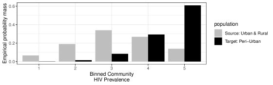
Figure 1: Empirical distribution of a covariate (binned community HIV prevalence with categories encoded by 1–6) in the two populations of the data concerning HIV risk prediction in a South African cohort.

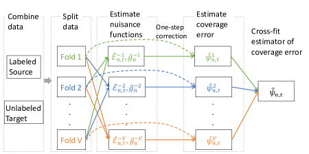
Figure 2: Overall procedure of the cross-fit one-step corrected estimator $\psi_{n,\tau}$ of the coverage error corresponding to the prediction set with threshold $\tau$, which forms the basis of our PredSet-1Step method.

In presence of covariate shift, prediction coverage guarantees may not hold if one assumes no covariate shift. Possible solutions have only recently formally been studied. Tibshirani et al. (2019) studied conformal prediction under covariate shift, assuming that the likelihood ratio is known a priori. Park et al. (2021) studied the PAC property of inductive conformal prediction (or, PAC prediction sets) under covariate shift. Their methods rely on knowing the covariate shift, i.e., the likelihood ratio of the covariate distribution in the target population to that in the source population, or on bounding its smoothness, which may not always be practical.

Cauchois et al. (2020) studied conformal prediction that is robust to a specified level of deviation of the target population from the source population. On the other hand, Lei and Candès (2021) studied conformal prediction under covariate shift without assuming that the likelihood ratio is known, and allowed estimation of this ratio instead. In this paper, we focus on the PAC property. In inductive conformal prediction under no covariate shift or known covariate shift, the PAC property can be obtained even though this method was developed to obtain marginal validity (see Vovk (2013) for the case without covariate shift and Park et al. (2021) for the case with known covariate shift). However, to our knowledge, PAC property results for inductive conformal prediction under completely unknown covariate shift have not yet been obtained.

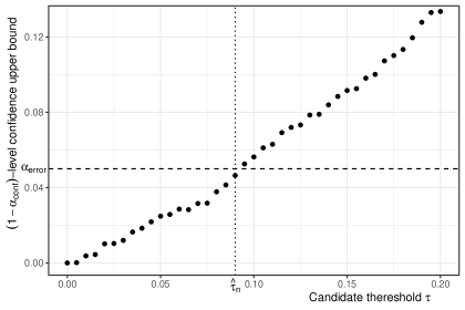
Figure S2: Illustration of threshold selection for prediction sets based on confidence upper bounds (CUBs). We first calculate approximate $(1-\alpha_{\mathrm{conf}})$-level confidence upper bounds for the coverage error of prediction sets corresponding to a set $\mathcal{T}_{n}$ of candidate thresholds. We then select the threshold $\hat{\tau}_{n}$ to be the maximum threshold in the candidate set $\mathcal{T}_{n}$ such that, for any threshold $\tau\in\mathcal{T}_{n}$ less than or equal to $\hat{\tau}_{n}$, the CUB corresponding to $\tau$ is less than $\alpha_{\mathrm{error}}$.

In this paper, we focus on achieving a PAC guarantee and show that PAC prediction sets under unknown covariate shift are uninformative. We next propose novel methods to construct prediction sets that are asymptotically PAC (APAC) as the sample size grows to infinity, with a convergence rate that we unravel. Our main method, PredSet-1Step, is based on asymptotically efficient one-step corrected estimators of the true coverage error and the associated Wald confidence intervals. The procedure to construct the estimator is illustrated in Figure 2, and the procedure to construct prediction sets afterwards is illustrated in Figure S2 in the Supplemental Material (see notations in the rest of this paper). PredSet-1Step heavily relies on semiparametric efficiency theory (see, e.g., Levit, 1974; Pfanzagl, 1985, 1990; Newey, 1990; Van Der Vaart, 1991; Bickel et al., 1993; van der Vaart and Wellner, 1996; Bickel et al., 1993; Chernozhukov et al., 2018; Kennedy, 2022) to obtain improved convergence rates. PredSet-1Step may also be used to construct asymptotically risk-controlling prediction sets (Bates et al., 2021).

This paper is organized as follows. We introduce the problem setup, present a negative result on PAC prediction sets, and present identification results under unknown covariate shift in Section 2. In Section 3, we provide an overview of our proposed methods. We describe our method to estimate the likelihood ratio, and present pathwise differentiability results of the miscoverage in the target population; akin to those of Hahn (1998). These form the basis of our proposed methods. We next describe our proposed PredSet-1Step method, which builds on cross-fitting/double machine learning (Schick, 1986; Chernozhukov et al., 2018), along with its theoretical properties, in Section 4. We show in Corollary 1 that PredSet-1Step yields APAC prediction sets with an error in the confidence level that is typically of order $n^{1/4}$ multiplied by the square root of the product of the convergence rates of estimators of two nuisance functions. These results are based on a novel bound on the difference between the realized and nominal coverage for Wald confidence intervals based on general asymptotically linear estimators (Theorem 4). We then present simulation studies in Section 5 and data analysis results in Section 6.

We present further results in the Supplemental Material. In Section S1, we propose an extension, PredSet-RS, of the rejection sampling method from Park et al. (2021). In Section S2, we present an alternative approach to PredSet-1Step, PredSet-TMLE, a targeted maximum likelihood estimation (TMLE) implementation of our efficient influence function based approach (Van der Laan and Rubin, 2006). We describe two methods to construct asymptotically risk-controlling prediction sets in Section S3. These methods are slightly modified versions of PredSet-1Step and PredSet-TMLE. The proofs of our theoretical results can be found in Section S7. We discuss the PAC property, comparing it with marginal validity, in Section S8. We finally clarify a connection between causal inference and covariate shift, based on which we may apply methods for covariate shift to obtain well-calibrated prediction sets for individual treatment effects (ITEs), in Section S9. Our proposed methods are implemented in an R package available at https://github.com/QIU-Hongxiang-David/APACpredset.

2 Problem setup and assumptions

2.1 Basic setting

Suppose one has observed labeled data from a source population, and unlabeled data from a target population. Denote a prototypical full (but unobserved) data point as $\bar{O}:=(A,X,Y)\sim\bar{P}^{0}$, where $A\in\{0,1\}$ is the indicator of the data point being drawn from the source population ($A=1$) or the target population ($A=0$), $X\in\mathcal{X}$ are the covariates, and $Y\in\mathcal{Y}$ is the outcome, label or dependent variable to be predicted. The observed data points are of the form $O:=(A,X,AY)\sim P^{0}$. In other words, in the observed data, outcomes (dependent variables) are observed only from the source population, and are missing from the target population (encoded as zero for notational convenience).

The observed data consists of $n$ independently and identically distributed (i.i.d.) observed data points $O_{i}\sim P^{0}$ ($i\in[n]:=\{1,2,\ldots,n\}$). Let $s:\mathcal{X}\times\mathcal{Y}\rightarrow\real$ be a given scoring function. For example, when $Y$ is a discrete variable, $s(x,y)$ may be an estimator of the probability of $Y=y$ given $X=x$ that has been trained from a held-out data set drawn from the source population. When $Y$ is a continuous variable, $s(x,y)$ may be an estimator of the conditional density of $Y$ at $y$ given $X=x$ or $-|y-\hat{y}(x)|$ for a given prediction model $\hat{y}$. The function $s$ can be arbitrary user-specified mapping. We treat $s$ as a fixed function throughout this paper; as shown in the above examples, in practice $s$ can be learned from a separate training set.

Let $\mathscr{B}\subseteq 2^{\mathcal{Y}}$ be the Borel $\sigma$-algebra of $\mathcal{Y}$, which is assumed to be a topological space. We refer to a map $C:\mathcal{X}\mapsto\mathscr{B}$ that assigns to each input $x\in\mathcal{X}$ a prediction set simply as a prediction set. Our goal is to construct a prediction set that is asymptotically probably approximately correct (APAC) in the target population. In other words, the prediction set should be asymptotically training-set-conditionally valid in the target population.

To be more precise, we first review a few related concepts. A prediction set $C$ is approximately correct in the target population if the true coverage error in the target population, ${\mathrm{Pr}}_{\bar{P}^{0}}(Y\notin C(X)\mid A=0)$, is less than or equal to a given target upper bound $\alpha_{\mathrm{error}}\in(0,1)$.

An estimated prediction set $\hat{C}$ constructed from the data is probably approximately correct (PAC) in the target population, with miscoverage level (also termed content) $\alpha_{\mathrm{error}}$ and confidence level $1-\alpha_{\mathrm{conf}}$ ($\alpha_{\mathrm{conf}}\in(0,1)$), if, for a $\hat{C}$-independent draw $(X,Y)$ from the target population,

$${\mathrm{Pr}}_{P^{0}}({\mathrm{Pr}}_{\bar{P}^{0}}(Y\notin\hat{C}(X)\mid A=0,\hat{C})\leq\alpha_{\mathrm{error}})\geq 1-\alpha_{\mathrm{conf}}.$$

In other words, $\hat{C}$ is PAC if we have confidence at least $1-\alpha_{\mathrm{conf}}$ that the true coverage error of the estimated prediction set $\hat{C}$ in the target population is below the desired level $\alpha_{\mathrm{error}}$.

Remark 1.

For conciseness in notations, in the rest of the paper, we may drop the distribution over which a probability is taken over when this distribution is clear (e.g., $\bar{P}^{0}$ or $P^{0}$) from the context. For example, we may write the above PAC guarantee as ${\mathrm{Pr}}({\mathrm{Pr}}(Y\notin\hat{C}(X)\mid A=0,\hat{C})\leq\alpha_{\mathrm{error}})\geq 1-\alpha_{\mathrm{conf}}$.

Methods to construct PAC prediction sets under covariate shift have been proposed when $Y$ is observed in data points drawn from the target population, or when the distribution shift from the source to the target population is known (Vovk, 2013; Park et al., 2020, 2021). RCPS have also been constructed, without considering covariate shift (Bates et al., 2021), while the problem with covariate shift has not been addressed, to our knowledge.

However, in our setting, neither the outcomes from the target population nor the distribution shift is known. Due to these unknown nuisance parameters, we have the following negative result on nontrivial prediction sets with a finite-sample marginal or PAC coverage guarantee.

Lemma 1.

Suppose that $\mathcal{X}$ and $\mathcal{Y}$ are Euclidean spaces. Let $\bar{{\mathcal{M}}}^{*}$ be the set of all distributions $\bar{P}^{0}$ on the full data point $\bar{O}$ such that unknown covariate shift is present (namely Conditions 1–3 in Section 2.2 hold), and the joint distribution of $(X,Y)$ is absolutely continuous with respect to the Lebesgue measure on $\mathcal{X}\times\mathcal{Y}$. Suppose that a (possibly randomized) prediction set $\hat{C}$ is PAC in the target population, that is,

$${\mathrm{Pr}}\left({\mathrm{Pr}}(Y\notin\hat{C}(X)\mid A=0,\hat{C})\leq\alpha_{\mathrm{error}}\right)\geq 1-\alpha_{\mathrm{conf}}$$

for all $\bar{P^{0}}\in\bar{{\mathcal{M}}}^{*}$. Then, for any $\bar{P^{0}}\in\bar{{\mathcal{M}}}^{*}$ and a.e. $y\in\mathcal{Y}$ with respect to the Lebesgue measure,

$${\mathrm{Pr}}(y\notin\hat{C}(X)\mid A=0)\leq\alpha_{\mathrm{error}}+\alpha_{\mathrm{conf}}.$$

If $\alpha_{\mathrm{error}}+\alpha_{\mathrm{conf}}<1$, Lemma 1 indicates that any PAC prediction set $\hat{C}$ in the target population under unknown covariate shift is essentially uninformative since it will contain almost any possible outcome with a nonzero probability for any data-generating mechanism. This lack of information can be clearly seen in the simple illustrative case where the support of $Y$ is and $Y\mathchoice{\mathrel{\hbox to0.0pt{$\displaystyle\perp$\hss}\mkern 2.0mu{\displaystyle\perp}}}{\mathrel{\hbox to0.0pt{$\textstyle\perp$\hss}\mkern 2.0mu{\textstyle\perp}}}{\mathrel{\hbox to0.0pt{$\scriptstyle\perp$\hss}\mkern 2.0mu{\scriptstyle\perp}}}{\mathrel{\hbox to0.0pt{$\scriptscriptstyle\perp$\hss}\mkern 2.0mu{\scriptscriptstyle\perp}}}X$. In this case, it would be desirable to obtain a PAC prediction set that outputs, for example, an estimated central or highest-density $1-\alpha_{\mathrm{error}}$ probability region of the distribution $Y\mid A=0$. However, Lemma 1 implies that such a PAC prediction set does not exist, and that a PAC prediction set would instead cover almost every $y\in\real$ with probability at least $1-(\alpha_{\mathrm{error}}+\alpha_{\mathrm{conf}})$ with respect to $X$. A similar negative result holds when $Y$ is discrete. We prove this lemma by (i) obtaining a similar negative result for prediction sets with finite-sample marginal coverage guarantees (Lemma S1 in the Supplemental Material), and (ii) using Theorem 2 and Remark 4 in Shah and Peters (2020). The proof can be found in Section S7.1 in the Supplemental Material.

Because of this negative result on finite-sample coverage guarantee, in this paper we choose to relax the validity criterion to an asymptotic one. It turns out that this way, we can account for unknown covariate shift. Recall that $n$ is the sample size used to estimate the prediction set.

Definition 1.

A sequence of estimated prediction sets $(\hat{C}_{n})_{n\geqslant 1}$ is asymptotically probably approximately correct (APAC) if

$${\mathrm{Pr}}({\mathrm{Pr}}(Y\notin\hat{C}_{n}(X)\mid A=0,\hat{C}_{n})\leq\alpha_{\mathrm{error}})\geq 1-\alpha_{\mathrm{conf}}+{\mathrm{o}}(1)$$ (1)

as $n\rightarrow\infty$, where the ${\mathrm{o}}(1)$ term tends to zero as $n\rightarrow\infty$.

In other words, a sequence of APAC prediction sets $\hat{C}_{n}$ is almost PAC for sufficiently large $n$. We will further quantify the magnitude of the $o(1)$ error in the confidence level. We use an estimated prediction set $\hat{C}_{n}$ and a sequence $(\hat{C}_{n})_{n\geqslant 1}$ interchangeably in this paper and may say that $\hat{C}_{n}$ is APAC. Further, we treat $\alpha_{\mathrm{error}}$ and $\alpha_{\mathrm{conf}}$ as fixed.

Remark 2.

Risk-controlling prediction set (RCPS) (Bates et al., 2021) is more general than but similar to PAC. Our proposed PredSet-1Step method can be readily applied to constructing asymptotic RCPS (ARCPS) with a slight modification. We introduce the concept of ARCPS and describe the modified method in Section S3 in the Supplemental Material.

Vovk (2013) derived the PAC property of inductive conformal predictors (Papadopoulos et al., 2002), and Park et al. (2020) presented a nested perspective (Vovk et al., 2005). While the formulations of Vovk (2013) and Park et al. (2020) are equivalent, we follow Park et al. (2020). For thresholds $\tau\in\bar{\real}$, where $\bar{\real}:=\real\cup\{\pm\infty\}$, we consider nested prediction sets (Vovk et al., 2005) of the form

$$C_{\tau}:x\mapsto\{y\in\mathcal{Y}:s(x,y)\geq\tau\}.$$

Since $C_{\tau_{1}}(x)\subseteqq C_{\tau_{2}}(x)$ for any $x$ and any $\tau_{1}\geqslant\tau_{2}$, typical measures of the size of $C_{\tau}$ (such as the cardinality or Lebesgue measure) are nonincreasing functions of $\tau$. Therefore, to obtain an APAC prediction set with a small size, given a finite set $\mathcal{T}_{n}\subseteqq\bar{\real}$ of candidate thresholds, we select a threshold $\hat{\tau}_{n}\in\mathcal{T}_{n}$ such that ${\mathrm{Pr}}({\mathrm{Pr}}(Y\notin C_{\hat{\tau}_{n}}(X)\mid A=0)\leq\alpha_{\mathrm{error}})\geq 1-\alpha_{\mathrm{conf}}+{\mathrm{o}}(1)$ and $\hat{\tau}_{n}$ is as large as possible. Our methods under this setting are our main contribution.

We summarize our main result informally. Formal results can be found in later sections. The algorithm to estimate the coverage error $\Psi_{\tau}(P^{0})={\mathrm{Pr}}(Y\notin C_{\tau}(X)\mid A=0)$ corresponding to the threshold $\tau$ used in PredSet-1Step is Algorithm 1. We will show in Corollary 1 that, under certain conditions, the prediction set $C_{\hat{\tau}^{\mathrm{1Step}}_{n}}$ with the threshold $\hat{\tau}^{\mathrm{1Step}}_{n}$ selected by PredSet-1Step is APAC:

$${\mathrm{Pr}}(\Psi_{\hat{\tau}^{\mathrm{1Step}}_{n}}(P^{0})\leq\alpha_{\mathrm{error}})\geq 1-\alpha_{\mathrm{conf}}-{\mathscr{C}}\Delta_{n,\varepsilon},$$

where ${\mathscr{C}}$ is an absolute positive constant and $\Delta_{n,\varepsilon}$ is typically of order $n^{1/4}$ multiplied by the square root of the product of the convergence rates of two nuisance function estimators. This corollary relies on a novel result on the convergence rate of Wald confidence interval coverage for general asymptotically linear estimators (Theorem 4). The result bounds the difference between the true and the nominal coverage by three error terms: (i) the difference between the estimator and a sample mean, (ii) the estimation error of the asymptotic variance, and (iii) the difference of the distribution of the sample mean from its limiting normal distribution.

Remark 3.

Beyond the APAC criterion, an alternative approach is to find a prediction set $C$ that approximately solves

$$\min\quad\mathrm{size}(C)\qquad\text{subject to}\quad\widehat{{\mathrm{Pr}}}(Y\notin C(X)\mid A=0)\leq\alpha_{\mathrm{error}},$$

where $\widehat{{\mathrm{Pr}}}(Y\notin C(X)\mid A=0)$ is an estimator of ${\mathrm{Pr}}(Y\notin C(X)\mid A=0)$ and $\mathrm{size}(C)$ is a measure of the size of the prediction set $C$. This approach has been considered in Yang et al. (2022), and generally results in smaller prediction sets than the APAC ones we consider in this paper. The reason is that the APAC guarantee requires approximately controlling the confidence level $1-\alpha_{\mathrm{conf}}$ to achieve the desired coverage error level $\alpha_{\mathrm{error}}$ over the data, which leads to some conservativeness. This difference can also been seen from the PAC guarantee in Yang et al. (2022) taking the form

$${\mathrm{Pr}}({\mathrm{Pr}}(Y\notin\hat{C}_{n}(X)\mid A=0,\hat{C}_{n})\leq\alpha_{\mathrm{error}}+{\mathrm{o}}_{p}(1))\geq 1-\alpha_{\mathrm{conf}}.$$ (2)

To distinguish from the APAC guarantee in (1), we call the guarantee in (2) a probably asymptotically approximately correct (PAAC) guarantee. The difference between APAC (1) and PAAC (2) is in the asymptotically vanishing approximation error: in APAC (1), the approximation is on the confidence level; in PAAC (2), the approximation is on the coverage error. This difference may seem subtle but has substantial impact on the performance of prediction sets satisfying these guarantees. We illustrate this difference by interpreting APAC (1) and PAAC (2) in words: APAC (1) states that, with confidence approaching the desired level $1-\alpha_{\mathrm{conf}}$, the true coverage error does not exceed the desired level $\alpha_{\mathrm{error}}$, but may frequently be a little conservative; PAAC (2) states that, with confidence at least $1-\alpha_{\mathrm{conf}}$, the true coverage error does not exceed the desired level $\alpha_{\mathrm{error}}$ by much, but may frequently exceed $\alpha_{\mathrm{error}}$ by a little. We also illustrate the difference in Figure 3. In some applications, having a high confidence guarantee on the desired level $\alpha_{\mathrm{error}}$ of true coverage error at a price of slight conservativeness may be desirable, for example, for safety purposes.

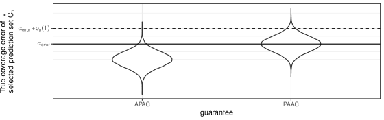
Figure 3: Exemplar sampling distributions of the true coverage error ${\mathrm{Pr}}(Y\notin\hat{C}_{n}(X)\mid A=0,\hat{C}_{n})$ of prediction sets $\hat{C}_{n}$ satisfying APAC and PAAC guarantees, respectively.

We conclude this section by introducing a few more notations. We use ${\mathscr{C}}$ to denote an absolute positive constant that may vary line by line. For two scalar sequences $(a_{n})_{n\geqslant 1}$ and $(b_{n})_{n\geqslant 1}$, we use $a_{n}\lesssim b_{n}$ to denote that for some constant ${\mathscr{C}}>0$ and all $n\geqslant 1$, $a_{n}\leq{\mathscr{C}}b_{n}$, and we define $\gtrsim$ similarly. We use $a_{n}\simeq b_{n}$ to denote that both $a_{n}\lesssim b_{n}$ and $a_{n}\gtrsim b_{n}$ hold. We also adopt the little-o and big-O notations. For a probability distribution $P$ and a scalar $p\geqslant 1$, we use $\|\cdot\|_{P,p}$ to denote the $L^{p}(P)$-norm of a function.

2.2 Identification

Without any further assumptions, it is impossible to estimate ${\mathrm{Pr}}(Y\notin C(X)\mid A=0)$ for an arbitrary prediction set $C$, since the joint distribution $(X,Y)\mid A=0$ of $(X,Y)$ in the target population cannot be identified due to $Y$ missing in the data. We make a few assumptions, following the standard setting in the covariate shift literature (see, e.g., Shimodaira, 2000; Quiñonero-Candela et al., 2009; Sugiyama and Kawanabe, 2012), so that ${\mathrm{Pr}}(Y\notin C(X)\mid A=0)$ can be identified as a functional of the true distribution $P^{0}$ on the observed data.

Let $P^{0}_{A}$ denote the marginal distribution of $A$ under $P^{0}$, $P^{0}_{X\mid a}$ denote the distribution of $X\mid A=a$ under $P^{0}$ for $a\in\{0,1\}$, $\bar{P}^{0}_{Y\mid x,a}$ the distribution of $Y\mid X=x,A=a$ under the full data distribution $\bar{P}^{0}$, and $P^{0}_{Y\mid x}:=\bar{P}^{0}_{Y\mid x,1}$. For any distribution $P$ of the observed data point $O$, we define these marginal and conditional distributions similarly and denote them with similar notations except that the superscript $0$ denoting $P^{0}$ is dropped. For example, $P_{X\mid a}$ stands for the distribution of $X\mid A=a$ under $P$. It will also be convenient to define the loss function

$$Z_{\tau}:(x,y)\mapsto{\mathbbm{1}}(y\notin C_{\tau}(x))$$

for any $\tau\in\bar{\real}$. Our first condition is:

Condition 1 (Data available from both populations).

$0<{\mathrm{Pr}}(A=1)<1$.

This condition ensures that data points from both source and target populations are collected in sufficient quantity, and that the conditional distributions introduced above are well defined. In practice, this condition requires that a reasonable amount of data from both populations is collected.

Next, we state the key covariate shift assumption (see, e.g., Shimodaira, 2000; Quiñonero-Candela et al., 2009; Sugiyama and Kawanabe, 2012), which is central to our paper.

Condition 2 (Covariate shift: Identical conditional outcome distribution).

The conditional distribution of $Y\mid X=x$ in the target population is identical to that in the source population for all $x\in\mathcal{X}$. Mathematically, $\bar{P}^{0}_{Y\mid x,1}=\bar{P}^{0}_{Y\mid x,0}=P^{0}_{Y\mid x}$.

Condition 2 is similar to the missing at random assumption in the missing data literature (see, e.g., Little and Rubin, 2019). It holds, for instance, if in the target we observe the same $Y$ (e.g., does a car face left or right), with $X$ from a different distribution (images from cities A vs B). Finally, we have an assumption to ensure that the target population overlaps with the source population.

Condition 3 (Dominance of covariate distributions).

The marginal distribution of $X$ in the target population, $P^{0}_{X\mid 0}$, is dominated by that in the source population, $P^{0}_{X\mid 1}$; that is, the Radon-Nikodym derivative $w_{0}:={\mathrm{d}}P^{0}_{X\mid 0}/{\mathrm{d}}P^{0}_{X\mid 1}$ is well defined.

We assume that Conditions 1–3 hold throughout this paper. For any distribution $P$ of the observed data point $O$ satisfying Condition 3 and any $\tau\in\bar{\real}$, we define the functionals

$$w_{P}:={\mathrm{d}}P_{X\mid 0}/{\mathrm{d}}P_{X\mid 1}\quad\text{and}\quad\mathcal{E}_{P,\tau}:x\mapsto{\mathrm{Pr}}_{P}(Y\notin C_{\tau}(X)\mid X=x,A=1).$$ (3)

We will also replace $P$ in the subscripts of these and other quantities with $0$ when referring to the functional components of $P^{0}$. Here, $w_{P}$ is the likelihood ratio between target and source covariate distributions under $P$, and $\mathcal{E}_{P,\tau}$ is the covariate-conditional coverage error of the prediction set $C_{\tau}$ in the source population. It is not hard to show that, under the distribution $\bar{P}$ of the complete but unobserved data, we can also express $\mathcal{E}_{P,\tau}$ in terms of the target population as $\mathcal{E}_{P,\tau}(x)={\mathrm{Pr}}_{\bar{P}}(Y\notin C_{\tau}(X)\mid X=x,A=0)$. Further, we define

$$\Psi^{\mathrm{Gcomp}}_{\tau}:P\mapsto{\mathbb{E}}_{P}[\mathcal{E}_{P,\tau}(X)\mid A=0]\quad\text{and}\quad\Psi^{\mathrm{weight}}_{\tau}:P\mapsto{\mathbb{E}}_{P}[w_{P}(X)Z_{\tau}(X,Y)\mid A=1].$$

One can verify that for $j\in\{{\mathrm{Gcomp}},{\mathrm{weight}}\}$,

$$\Psi^{j}_{\tau}(P^{0})={\mathrm{Pr}}_{\bar{P}^{0}}(Y\notin C_{\tau}(X)\mid A=0).$$ (4)

In other words, although $\Psi^{\mathrm{Gcomp}}_{\tau}(P^{0})$ and $\Psi^{\mathrm{weight}}_{\tau}(P^{0})$ take as inputs different components of $P^{0}$, both correspond to the same functional of $P^{0}$, the coverage error of the prediction set $C_{\tau}$ in the target population. We will use $\Psi_{\tau}$ to denote these two functionals when we need not distinguish their mathematical expressions. In other words, $\Psi_{\tau}(P^{0})$ equals the probability that $Y\notin C_{\tau}(X)$ in the “covariate shifted” population where $A=0$:

$$\Psi_{\tau}(P^{0})={\mathrm{Pr}}_{\bar{P}^{0}}(Y\notin C_{\tau}(X)\mid A=0).$$ (5)

Borrowing terminology from causal inference and missing data, we refer to $\Psi^{\mathrm{Gcomp}}_{\tau}(P^{0})$ and $\Psi^{\mathrm{weight}}_{\tau}(P^{0})$ as the G-computation formula and the weighted formula, respectively.

Remark 4.

Both $\Psi^{\mathrm{Gcomp}}_{\tau}$ and $\Psi^{\mathrm{weight}}_{\tau}$ take as inputs only certain components of the distribution rather than the entire distribution, and hence may be computed as long as the relevant components are defined. For example, $\Psi^{\mathrm{Gcomp}}_{\tau}(P)$ is defined if the distribution $P_{X\mid 0}$ and $\mathcal{E}_{P,\tau}$ are defined. We will specify only the required components when defining our estimators.

Remark 5.

There is a connection between counterfactuals in causal inference and covariate shift, as pointed out in Lei and Candès (2021). We discuss this connection in more detail in Section S9 in the Supplemental Material.

3 Overview and preliminaries of proposed method

In all methods we propose, we assume that a finite set $\mathcal{T}_{n}$ of candidate thresholds is given, with a cardinality that may grow to infinity with $n$. Since, as a function of $\tau$, there are at most $n+1$ versions of the observed miscoverage indicators $\{Z_{\tau}(X_{i},Y_{i})={\mathbbm{1}}(s(X_{i},Y_{i})<\tau),i\in[n]\}$ in any data set, each corresponding to a threshold in the set $\{s(X_{i},Y_{i}):i\in[n]\}\cup\infty$, this assumption is not stringent.

Our general strategy is to construct an asymptotically valid $(1-\alpha_{\mathrm{conf}})$-confidence upper bound (CUB) for $\Psi_{\tau}(P^{0})$ for each threshold $\tau\in\mathcal{T}_{n}$, and select the largest threshold $\hat{\tau}_{n}\in\mathcal{T}_{n}$ such that, for any candidate threshold less than or equal to $\hat{\tau}_{n}$, the corresponding CUB is less than $\alpha_{\mathrm{error}}$. This procedure is illustrated in Figure S2 in the Supplemental Material. To construct accurate approximate confidence intervals (CIs), we rely on semiparametric efficiency theory (Bickel, 1982; Pfanzagl, 1985, 1990; Newey, 1990; Van Der Vaart, 1991; Bickel et al., 1993; van der Vaart, 1998; Bickel et al., 1993; Kennedy, 2022).

3.1 Estimation of nuisance functions

For a given threshold $\tau$, we will see in Section 3.2 that it is helpful to estimate nuisance functions corresponding to the pointwise coverage error

$$\mathcal{E}_{0,\tau}=\mathcal{E}_{P^{0},\tau}:x\mapsto{\mathrm{Pr}}_{P^{0}}(Y\notin C_{\tau}(X)\mid X=x,A=1)$$ (6)

and the covariate shift likelihood ratio $w_{0}$ from Condition (3). An estimator $\mathcal{E}_{n,\tau}$ of $\mathcal{E}_{0,\tau}$ may be obtained with standard classification or regression algorithms in the subsample from the source population with dependent variable $Z_{\tau}(X,Y)$ and covariate $X$.

However, for the estimation of the likelihood ratio $w_{0}$, we opt for a re-parametrization to a classification problem. Inspired by Friedman (2004), Bickel et al. (2007), Sugiyama et al. (2008), and Menon and Ong (2016), we use the following observation from Bayes’ Theorem. For any distribution $P$ of the observed data point $O$ satisfying Condition 3, define $g_{P}:x\mapsto[0,1]$ and $\gamma_{P}\in(0,1)$ via

$$g_{P}(x):={\mathrm{Pr}}_{P}(A=1\mid X=x),\qquad\gamma_{P}:={\mathrm{Pr}}_{P}(A=1).$$ (7)

We define $g_{0}$ and $\gamma_{0}$ similarly for $P^{0}$:

$$g_{0}(x):={\mathrm{Pr}}_{P^{0}}(A=1\mid X=x),\qquad\gamma_{0}:={\mathrm{Pr}}_{P^{0}}(A=1).$$ (8)

Following terminology in causal inference, we call $g_{0}$ the propensity score function (Rosenbaum and Rubin, 1983). When referring to generic propensity score functions and probabilities, we will write $g$ and $\gamma$ instead of $g_{P}$ and $\gamma_{P}$. For any propensity score function $g$ and any probability $\gamma\in(0,1)$, we define $\mathscr{W}(g,\gamma):\mathcal{X}\to[0,\infty)$ as

$$\mathscr{W}(g,\gamma)(x):=\frac{1-g(x)}{g(x)}\frac{\gamma}{1-\gamma}.$$ (9)

Bayes’ theorem directly shows that

$$w_{0}(x)=\mathscr{W}(g_{0},\gamma_{0})(x).$$ (10)

We will use this reparameterization through the rest of this paper. We can estimate $\gamma_{0}$ by $\gamma_{n}$ obtained from the empirical distribution. Further, we may estimate $g_{0}$ by $g_{n}$ obtained with standard classification or regression algorithms with dependent variable $A$ and covariate $X$. In our experience, existing classification techniques are more flexible in our setting than density estimation methods. For instance, density estimation procedures might need adjustment according to the support of variables in $X$ (e.g., bounded continuous, unbounded continuous, discrete, a mixture, etc.), while most classification methods need not make this distinction.

3.2 Pathwise differentiability

We next present results on pathwise differentiability of the error rate parameter $\Psi_{\tau}$ with respect to ${\mathcal{M}}$, a model that is nonparametric at $P^{0}$, which are akin to those of Hahn (1998); see also (Levit, 1974; Bickel, 1982; Pfanzagl, 1985, 1990; Newey, 1990; Van Der Vaart, 1991; Bickel et al., 1993; van der Vaart, 1998; Bickel et al., 1993). We first briefly describe the intuition behind these terminologies. Consider a generic one-dimensional parametric submodel $(P^{\varepsilon}_{H})_{\varepsilon\in\real}$ satisfying ${\mathrm{d}}P^{\varepsilon}_{H}/{\mathrm{d}}P^{0}(o)\approx 1+\varepsilon H(o)$ for some function $H$ with ${\mathbb{E}}_{P^{0}}[H(O)]=0$ and finite variance. We only consider regular parametric submodels (see, e.g., Newey, 1990; Bickel et al., 1993, for more details). The function $H$ is called the score function of this submodel. We say that a model ${\mathcal{M}}$ is nonparametric at $P^{0}$ if, for any function $H$ with mean zero and finite variance, $P^{\varepsilon}_{H}\in{\mathcal{M}}$ for $\varepsilon$ sufficiently close to zero. Roughly speaking, $H$ encodes the direction of local perturbations of $P^{0}$ in the submodel, and a nonparametric model allows any perturbation of $P^{0}$.

We focus on nonparametric models in the main text, in which case no information about $P^{0}$ is known. In particular, the estimator $(\mathcal{E}_{n,\tau},w_{n})$ of $(\mathcal{E}_{0,\tau},w_{0})$ may converge in probability in an $L^{2}(P^{0})$ sense at a rate slower than or equal to $n^{-1/2}$. This rate is typically slower than the parametric rate $n^{-1/2}$ as long as the covariate $X$ has continuous components.

A parameter $\Psi:{\mathcal{M}}\rightarrow\real$ is pathwise differentiable if ${\mathrm{d}}\Psi(P^{\varepsilon}_{H})/{\mathrm{d}}\varepsilon|_{\varepsilon=0}={\mathbb{E}}_{P^{0}}[H(O)D(O)]$ for some function $D$ with ${\mathbb{E}}_{P^{0}}[D(O)]=0$ and finite variance. This function $D$ is called a gradient of the parameter $\Psi$ at $P^{0}$, since it characterizes the local change in the value of the parameter corresponding to a perturbation of $P^{0}$. We can then heuristically expand $\Psi(P^{\varepsilon}_{H})$ around $\Psi(P^{0})$:

$$\Psi(P^{\varepsilon}_{H})-\Psi(P^{0})\approx\varepsilon\int H(o)D(o)P^{0}({\mathrm{d}}o)$$

$$=\int(1+\varepsilon H(o))D(o)P^{0}({\mathrm{d}}o)-\int D(o)P^{0}({\mathrm{d}}o)\approx\int D(o)(P^{\varepsilon}_{H}-P^{0})({\mathrm{d}}o).$$ (11)

In nonparametric models, the gradient $D$ is unique and also called the canonical gradient. The above explanation is informal, and we refer the readers to Section S7.2 in the Supplemental Material and to Levit (1974); Pfanzagl (1985, 1990); Bickel et al. (1993) for more details. The pathwise differentiability of an estimator is closely related to efficiency, and is crucial for the construction of a root-$n$-consistent and asymptotically normal estimator.

An estimator is asymptotically efficient under a nonparametric model if it equals the estimand plus the sample mean of the canonical gradient, up to an error ${\mathrm{o}}_{p}(n^{-1/2})$. An asymptotically efficient estimator is root-$n$ consistent and has the smallest possible asymptotic variance among a large class of estimators called regular estimators (see, e.g., Section 8.5 in van der Vaart, 1998). Hence, the result on pathwise differentiability of $\Psi_{\tau}$ forms the basis of constructing efficient estimators of $\Psi_{\tau}(P^{0})$, based on which approximate CUBs can be constructed under a nonparametric model.

Now we return to our prediction set problem. Consider an arbitrary function $\mathcal{E}$ defined on $\mathcal{X}$ with range contained in $[0,1]$, any scalar $\gamma\in(0,1)$, and any positive scalar $\pi$. For each $\tau\in\bar{\real}$, with $o:=(a,x,y)$, we define the function

$$D_{\tau}(P,g,\gamma):o \mapsto\frac{a}{\gamma_{P}}\mathscr{W}(g,\gamma)(x)\left\{Z_{\tau}(x,y)-\mathcal{E}_{P,\tau}(x)\right\}+\frac{1-a}{1-\gamma_{P}}[\mathcal{E}_{P,\tau}(x)-\Psi^{\mathrm{Gcomp}}_{\tau}(P)].$$ (12)

For notational convenience, we suppress the dependence of this gradient function on the target parameter $\Psi_{\tau}(P)$; this dependence is implicit through the dependence on $P$.

We require an additional bounded likelihood ratio condition, which is standard in the literature on covariate shift (Shimodaira, 2000; Quiñonero-Candela et al., 2009; Sugiyama and Kawanabe, 2012).

Condition 4 (Bounded likelihood ratio).

There exists a constant $B<\infty$ such that $\sup_{x\in\mathcal{X}}w_{0}(x)<B$. Equivalently, there exists a constant $\delta\in(0,1)$ such that the propensity score is bounded away from zero, namely $\inf_{x\in\mathcal{X}}g_{0}(x)>\delta$. Here, $\delta$ may be taken as $\gamma_{0}/(B(1-\gamma_{0})+1)$.

Under Condition 4, it holds that $\sup_{\tau\in\bar{\real}}{\mathbb{E}}_{P^{0}}[D_{\tau}(P^{0},g_{0},\gamma_{0})(O)^{2}]<\infty$, because $Z_{\tau}$ is bounded. The pathwise differentiability of $\Psi$ is presented in the following theorem, which is a version of the results of Hahn (1998) in causal inference.

Theorem 2 (Pathwise differentiability of $\Psi_{\tau}$).

Under Conditions 1–4, for each $\tau\in\bar{\real}$, the functional $\Psi_{\tau}$ from (5), where $\Psi_{\tau}(P^{0})={\mathrm{Pr}}(Y\notin C_{\tau}(X)\mid A=0)$ is the coverage error in the target, “covariate shifted” population with $A=0$, is pathwise differentiable at $P^{0}$ relative to ${\mathcal{M}}$ with canonical gradient $D_{\tau}(P^{0},g_{0},\gamma_{0})$ from (12).

The proof of Theorem 2 is related to the proof of Theorem 1 in Hahn (1998): with $1-A$ being the treatment indicator $D$ in Hahn (1998), ${\mathbbm{1}}(Y\notin\hat{C}_{\tau}(X))$ being the counterfactual outcome $Y_{0}$ in Hahn (1998), $\Psi_{\tau}(P^{0})$ can be written as the mean counterfactual outcome ${\mathbb{E}}[Y_{0}\mid D=1]$ in the treated group in Hahn (1998). Estimating this is the main challenge in estimating the average treatment effect ${\mathbb{E}}[Y_{1}-Y_{0}\mid D=1]$ on the treated; the canonical gradient of ${\mathbb{E}}[{\mathbbm{1}}(Y\notin\hat{C}_{\tau}(X))\mid A=0]$ can be calculated using arguments similar to the proof of Theorem 1 in Hahn (1998). We provide the proof in Section S7.2 in the Supplemental Material. Since both nuisance functions $\mathcal{E}_{0,\tau}$ and $w_{0}$ appear in the canonical gradient, it is helpful to estimate both functions in order to construct asymptotically efficient estimators of $\Psi_{\tau}(P^{0})$ as well as asymptotically valid CUBs. As is known in the sieve estimation literature (see, e.g., Chen, 2007; Qiu et al., 2021; Shen, 1997) and other nonparametric inference literature (see, e.g., Bickel and Ritov, 2003; Newey et al., 1998, 2004), it is possible to only estimate—for example—$\mathcal{E}_{0,\tau}$, with specific nonparametric methods, and still obtain an asymptotically efficient estimator of $\Psi_{\tau}(P^{0})$. In this paper, we do not take these approaches and propose methods that require estimating both nuisance functions in our procedures to allow for the most generality and flexibility in choosing estimators of nuisance functions.

Remark 6.

The pathwise differentiability of $\Psi_{\tau}$ does not use that the loss function $Z_{\tau}(x,y)={\mathbbm{1}}(y\notin C_{\tau}(x))$ is binary. Therefore, our approach works for general loss functions, and we may construct asymptotically efficient estimators in that setting. Then we can construct asymptotically efficient estimators for the true risk that corresponds to a general loss function for a prediction set under covariate shift. In particular, PredSet-1Step may be used with slight modifications for the estimation of the conditional risk function $\mathcal{E}_{0,\tau}$ for general losses. We present the corresponding results for constructing ARCPS in Section S3 in the Supplemental Material.

4 PredSet-1Step

In this section, we describe the PredSet-1Step method, based on an asymptotically efficient one-step corrected estimator of $\Psi_{\tau}(P^{0})$, along with its main theoretical properties. For each candidate $\tau\in\mathcal{T}_{n}$, we first construct an asymptotically efficient estimator $\hat{\psi}_{n,\tau}$ of $\Psi_{\tau}(P^{0})$, and then obtain a consistent estimator $\hat{\sigma}_{n,\tau}^{2}$ of the asymptotic variance $\hat{\sigma}_{0,\tau}^{2}$ of $\hat{\psi}_{n,\tau}$. We finally construct a Wald CUB based on $\hat{\psi}_{n,\tau}$ and $\hat{\sigma}_{n,\tau}^{2}$. We select thresholds $\tau\in\mathcal{T}_{n}$ for prediction sets based on the CUBs. We next describe each step in more detail.

4.1 Cross-fit one-step corrected estimator

In this section, we describe a cross-fit one-step corrected estimator of $\Psi_{\tau}(P^{0})$ for a given $\tau$. After obtaining an estimator $\hat{\mathcal{E}}_{n,\tau}$ of $\mathcal{E}_{0,\tau}$ via parametric (e.g., logistic regression, neural nets) or nonparametric methods, it might be tempting to estimate $\Psi_{\tau}(P^{0})$ by the mean of $\hat{\mathcal{E}}_{n,\tau}(X)$ among observations from the target population. In other words, $\hat{\mathcal{E}}_{n,\tau}$ is plugged into $\Psi^{\mathrm{Gcomp}}$. However, in general, this plug-in estimator may not be rate-optimal and may invalidate subsequent CUB construction and APAC guarantees. The reason is a bias term that may dominate the convergence of this estimator.

Fortunately, this excessive bias can be reduced by a one-step correction on the standard plug-in estimator (see, e.g., Theorem 4 in Chapter 3 of Le Cam (1969) for early development of this idea for parametric models, and Pfanzagl (1985); Schick (1986) as well as Section 25.8 in van der Vaart (1998) for more modern generalizations to semi-/non-parametric models.) We further incorporate cross-fitting into the procedure to relax restrictions on the techniques used to estimate nuisance functions $\mathcal{E}_{0,\tau}$ and $g_{0}$. This technique improves performance in small to moderate samples; see e.g., Kennedy (2022) for a review. More generally, such sample splitting ideas date back at least to Hajek (1962).

Suppose that the data is split into $V$ folds of approximately equal size completely at random. We assume that $V\geq 2$ is fixed. Common choices of $V$ include five and ten. Let $I_{v}\subseteqq[n]$ denote the index set of observations in fold $v\in[V]$. We use $P^{n,v}$ to denote the empirical distribution of data in fold $v$. We also use $P_{A}^{n,v}$ and $P_{X\mid a}^{n,v}$ to denote the empirical distribution of $A$ and $X\mid A=a$ corresponding to data in fold $v$.

For each $\tau$, let $\hat{\mathcal{E}}_{n,\tau}^{-v}$ denote a flexible estimator of $\mathcal{E}_{0,\tau}$ obtained from data points out of fold $v$ via, for example, standard regression or supervised statistical learning tools. We also use $g_{n}^{-v}$ to denote a flexible estimator of $g_{0}$ obtained from data points out of fold $v$. We define

$$\hat{\gamma}_{n}^{v}:={\mathrm{Pr}}_{P^{n,v}}(A=1).$$ (13)

We construct a cross-fit one-step corrected estimator using Algorithm 1. Direct calculation shows that the one-step corrected estimator $\hat{\psi}_{n,\tau}^{v}$ for fold $v$ from (15) equals

$$\Psi^{\mathrm{Gcomp}}_{\tau}(\hat{P}_{\tau}^{n,v})+\frac{1}{|I_{v}|}\sum_{i\in I_{v}}D_{\tau}(\hat{P}_{\tau}^{n,v},\hat{g}_{n}^{-v},\hat{\gamma}_{n}^{v})(O_{i}).$$ (14)

The key one-step correction in (14) based on the canonical gradient is similar to a correction based on a linear approximation using the gradient in (12) at the estimated distribution $\hat{P}_{\tau}^{n,v}$. We roughly describe the intuition below in an informal manner, and refer the readers to Section S7.3 in the Supplemental Material for technical details. Following (11), we expand $\Psi(P^{0})$ around $\Psi(\hat{P}_{\tau}^{n,v})$:

$$\Psi(P^{0}) \approx\Psi(\hat{P}_{\tau}^{n,v})+\int D_{\tau}(\hat{P}_{\tau}^{n,v},\hat{g}_{n}^{-v},\hat{\gamma}_{n}^{v})(o)(P^{0}-\hat{P}_{\tau}^{n,v})({\mathrm{d}}o)$$

$$=\Psi(\hat{P}_{\tau}^{n,v})+{\mathbb{E}}_{P^{0}}[D_{\tau}(\hat{P}_{\tau}^{n,v},\hat{g}_{n}^{-v},\hat{\gamma}_{n}^{v})(O)],$$

where, in the expectation in the second line, we treat $(\hat{P}_{\tau}^{n,v},\hat{g}_{n}^{-v},\hat{\gamma}_{n}^{v})$ as fixed. The second equality follows because a gradient at $P$ has mean zero under $P$. Since the above correction term is unknown, we replace the expectation under $P^{0}$ with the empirical mean and thus find the one-step correction in (14). This idea is illustrated in Figure 4. This one-step correction is crucial to ensure root-$n$ consistency and asymptotic normality of the estimator, as we illustrate in a simulation shown in Figure S3 in the Supplemental Material.

Algorithm 1 Cross-fit one-step estimator of coverage error $\Psi_{\tau}(P^{0})$ used in PredSet-1Step

1:for $v\in[V]$ do Estimate $g_{0}$ by $\hat{g}_{n}^{-v}$ using data out of fold $v$.  

2:for $v\in[V]$ and $\tau\in\mathcal{T}_{n}$ do Estimate $\mathcal{E}_{0,\tau}$ by $\hat{\mathcal{E}}_{n,\tau}^{-v}$ using data out of fold $v$.  

3:for $v\in[V]$ and $\tau\in\mathcal{T}_{n}$ do $\triangleright$ (Obtain a one-step corrected estimator for fold $v$)

4:     Let $\hat{P}_{\tau}^{n,v}$ be a distribution with the following components: (i) marginal distribution of $A$ being $P_{A}^{n,v}$, (ii) conditional distribution of $X\mid A=0$ being $P_{X\mid 0}^{n,v}$, and (iii) distribution of $Z_{\tau}\mid X,A=1$ defined by $\hat{\mathcal{E}}_{n,\tau}^{-v}$

5:     Let $|I_{v}|$ be the cardinality of the index set $I_{v}$. Set

$$\hat{\psi}_{n,\tau}^{v}:=\frac{\sum_{i\in I_{v}}(1-A_{i})\hat{\mathcal{E}}_{n,\tau}^{-v}(X_{i})}{\sum_{i\in I_{v}}(1-A_{i})}+\frac{1}{|I_{v}|}\sum_{i\in I_{v}}\frac{A_{i}}{\hat{\gamma}_{n}^{v}}\mathscr{W}(\hat{g}_{n}^{-v},\hat{\gamma}_{n}^{v})[Z_{\tau}(X_{i},Y_{i})-\hat{\mathcal{E}}_{n,\tau}^{-v}(X_{i})].$$ (15)

6:for $\tau\in\mathcal{T}_{n}$ do Obtain the cross-fit one-step corrected estimator for threshold $\tau$:

$$\hat{\psi}_{n,\tau}:=\frac{1}{n}\sum_{v=1}^{V}|I_{v}|\hat{\psi}_{n,\tau}^{v}.$$ (16)

 

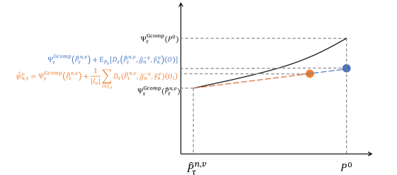
Figure 4: Illustration of the idea behind the one-step correction in (14). In this figure, $\Psi^{\mathrm{Gcomp}}_{\tau}(\hat{P}_{\tau}^{n,v})+{\mathbb{E}}_{P^{0}}[D_{\tau}(\hat{P}_{\tau}^{n,v},\hat{g}_{n}^{-v},\hat{\gamma}_{n}^{v})(O)]$ is the ideal/oracle first-order approximation to the estimand $\Psi^{\mathrm{Gcomp}}_{\tau}(P^{0})$ at the naïve plug-in estimator $\Psi^{\mathrm{Gcomp}}_{\tau}(\hat{P}_{\tau}^{n,v})$; $\hat{\psi}_{n,\tau}^{v}$ is the one-step corrected estimator.

We require two additional conditions on $\hat{g}_{n}^{-v}$ and $\hat{\mathcal{E}}_{n,\tau}^{-v}$ for $\hat{\psi}_{n,\tau}$ to be asymptotically efficient.

Condition 5 (Bounded propensity score estimator).

For some non-negative sequence $(q_{n})_{n\geq 0}$ tending to zero as $n\to\infty$, with probability $1-q_{n}$, $\inf_{v\in[V],x\in\mathcal{X}}\hat{g}_{n}^{-v}(x)>\delta$, where $\delta$ is the constant introduced in Condition 4.

Typically, with appropriate regularization to avoid overfitting, the estimator $\hat{g}_{n}^{-v}$ of the propensity score is bounded away from zero except in extremely ill-posed datasets. These occur with extremely small probability (for example, if the covariate $X$ is discrete and for some $x$, all observations with $X=x$ are from the target population). Moreover, the user can always truncate the estimator to be bounded away from zero, in which case $q_{n}=0$. Thus we often expect $q_{n}$ in Condition 5 to decrease to zero at a much faster rate than the convergence rates of the nuisance function estimators in Condition 6. This does not have an effect on the asymptotic efficiency of the cross-fit one-step estimator $\hat{\psi}_{n,\tau}$, but it will affect the Wald confidence interval coverage in the next subsection. Recall that $\|\cdot\|_{P,p}$ stands for the $L^{p}(P)$-norm of a function. Our condition for nuisance estimators is as follows.

Condition 6 (Sufficient rates for nuisance estimators).

The following conditions hold:

$${\mathbb{E}}_{P^{0}}\sup_{v\in[V],\tau\in\mathcal{T}_{n}}\|\hat{\mathcal{E}}_{n,\tau}^{-v}-\mathcal{E}_{0,\tau}\|_{P^{0}_{X\mid 0},2}={\mathrm{o}}(1),\quad{\mathbb{E}}_{P^{0}}\sup_{v\in[V]}\|(1-\hat{g}_{n}^{-v})/\hat{g}_{n}^{-v}-(1-g_{0})/g_{0}\|_{P^{0}_{X\mid 0},2}={\mathrm{o}}(1),$$

$${\mathbb{E}}_{P^{0}}\sup_{v\in[V],\tau\in\mathcal{T}_{n}}\int\left|\left\{\frac{1-\hat{g}_{n}^{-v}(x)}{\hat{g}_{n}^{-v}(x)}-\frac{1-g_{0}(x)}{g_{0}(x)}\right\}\left\{\hat{\mathcal{E}}_{n,\tau}^{-v}(x)-\hat{\mathcal{E}}_{0,\tau}(x)\right\}\right|P^{0}_{X\mid 1}({\mathrm{d}}x)={\mathrm{o}}(n^{-1/2}).$$

By the Cauchy-Schwarz inequality, a sufficient condition for the last equation in Condition 6 is the following:

$${\mathbb{E}}_{P^{0}}\sup_{v\in[V],\tau\in\mathcal{T}_{n}}\left\|\frac{1-\hat{g}_{n}^{-v}}{\hat{g}_{n}^{-v}}-\frac{1-g_{0}}{g_{0}}\right\|_{P^{0}_{X\mid 1},2}\left\|\hat{\mathcal{E}}_{n,\tau}^{-v}-\mathcal{E}_{0,\tau}\right\|_{P^{0}_{X\mid 1},2}={\mathrm{o}}(n^{-1/2}).$$

Therefore, a sufficient condition is that both nuisance estimators converge at a rate faster than $n^{-1/4}$. Thus we allow for much slower rates than the parametric root-$n$ rate. This ${\mathrm{o}}(n^{-1/4})$ rate requirement is only a sufficient condition and is by no means necessary. Condition 6 is satisfied even if one nuisance estimator converges very slowly, as long as the other nuisance estimator converges sufficiently fast to compensate for this slow convergence. We require convergence of the estimator $\mathcal{E}_{n,\tau}^{-v}$ uniformly over $\tau\in\mathcal{T}_{n}$ to establish uniform asymptotic efficiency in Theorem 3 below. Though this assumption on convergence is stronger than assumptions typically needed to obtain efficient estimators, it may not be stringent. We illustrate this with an example in Section S5 in the Supplemental Material.

Remark 7.

The aforementioned phenomenon that one convergence rate can compensate for the other is similar to the mixed bias property, which is frequently observed for semiparametrically or nonparametrically efficient estimators (Rotnitzky et al., 2021). The mixed bias property often leads to double robustness. An estimator is doubly robust if it is still consistent even when one nuisance function, but not the other, is estimated inconsistently (see, e.g., the rejoinder to discussions of Scharfstein et al. (1999), Robins (2000), and Bang and Robins (2005)). This double robustness property also holds for our estimator $\hat{\psi}_{n,\tau}$ of coverage error $\Psi_{\tau}(P^{0})$, similarly to the method in Yang et al. (2022). In other words, $\hat{\psi}_{n,\tau}$ is consistent for $\Psi_{\tau}(P^{0})$ even if either $\mathcal{E}_{0,\tau}$ or $g_{0}$ is estimated inconsistently, in which case Condition 6 fails. We do, however, generally require Condition 6 to hold for our proposed PredSet-1Step method except for special cases. The reason is that PredSet-1Step further relies on asymptotically valid CUBs, which rely on the asymptotic normality of $\hat{\psi}_{n,\tau}$. If a nuisance function is estimated inconsistently and thus Condition 6 fails, even though $\hat{\psi}_{n,\tau}$ is still consistent for $\Psi_{\tau}(P^{0})$, $\hat{\psi}_{n,\tau}$ is no longer asymptotically normal in general. In this case, it is challenging, if possible at all, to construct asymptotically valid CUB. We discuss special cases where PredSet-1Step is doubly robust under Condition S5 or S6 in Section S4 in the Supplemental Material. In particular, when one nuisance function is known, our proposed procedure remains valid with the known nuisance function plugged in.

This leads to our second result.

Theorem 3 (Asymptotic efficiency of cross-fit one-step corrected estimator).

Under Conditions 1–6, the one-step corrected cross-fit estimator $\hat{\psi}_{n,\tau}$ from (16) is an asymptotically nonparametrically efficient estimator of the coverage error $\Psi_{\tau}(P^{0})={\mathrm{Pr}}(Y\notin C_{\tau}(X)\mid A=0)$ from (5), in the target, “covariate shifted” population where $A=0$. Moreover, with the gradient $D_{\tau}$ from (12), the propensity score $g_{0}$ and the probability $\gamma_{0}$ of $A=1$ from (8), and the conditional coverage error rate $\mathcal{E}_{0,\tau}$ from (6),

$$\sup_{\tau\in\mathcal{T}_{n}}\left|\hat{\psi}_{n,\tau}-\Psi_{\tau}(P^{0})-\frac{1}{n}\sum_{i=1}^{n}D_{\tau}(P^{0},g_{0},\gamma_{0})(O_{i})\right|={\mathrm{o}}_{p}(n^{-1/2}).$$

Theorem 3 states the same asymptotic efficiency claim that is implied by the general result Theorem 3.1 and the more concrete result Theorem 5.1 in Chernozhukov et al. (2018). See also Proposition 2 in Kennedy (2022). One difference is that Theorem 3 concerns a uniform efficiency claim over $\tau\in\mathcal{T}_{n}$, which is implied by pointwise efficiency and the uniform rate condition 6; another difference arises in the proof due to the different estimation strategies for the nuisance parameter $\gamma_{0}$. The proof of Theorem 3 can be found in Section S7.3 in the Supplemental Material. As explained in Section 3.2, this result implies that the one-step corrected estimator enjoys a desirable optimality property: it has the smallest possible asymptotic variance, among all regular estimators, under the nonparametric model ${\mathcal{M}}$.

Remark 8.

Although $\hat{\psi}_{n,\tau}$ is consistent for $\Psi_{\tau}(P^{0})\in[0,1]$, this estimator itself may fall outside of the interval $[0,1]$. This possibility may harm the interpretation of $\hat{\psi}_{n,\tau}$ as an estimator of a probability. We may project $\hat{\psi}_{n,\tau}$ onto $[0,1]$, or instead use the targeted minimum-loss based estimator (TMLE) (Van der Laan and Rubin, 2006; Van der Laan and Rose, 2018). We present the method based on TMLE, PredSet-TMLE, in Section S2 in the Supplemental Material.

4.2 Wald CUB and selection of threshold

To construct Wald CUBs based on $\hat{\psi}_{n,\tau}$ using Theorem 3, we need to estimate the asymptotic variance $\sigma^{2}_{0,\tau}:={\mathbb{E}}_{P^{0}}[D_{\tau}(P^{0},g_{0},\gamma_{0})(O)^{2}]$. We propose to use a plug-in estimator based on sample splitting. Let

$$(\hat{\sigma}_{n,\tau}^{v})^{2}:=\frac{1}{|I_{v}|}\sum_{i\in I_{v}}D_{\tau}(\hat{P}_{\tau}^{n,v},\hat{g}_{n}^{-v},\hat{\gamma}_{n}^{v})(O_{i})^{2}\qquad\textnormal{ and }\qquad\hat{\sigma}_{n,\tau}:=\left[\frac{1}{n}\sum_{v=1}^{V}|I_{v}|(\hat{\sigma}_{n,\tau}^{v})^{2}\right]^{1/2}.$$ (17)

We propose to use $\hat{\sigma}_{n,\tau}/\sqrt{n}$ as the standard error when constructing a $(1-\alpha_{\mathrm{conf}})$-Wald CUB of $\Psi_{\tau}(P^{0})$. That is, we propose to use $\hat{\psi}_{n,\tau}+z_{\alpha_{\mathrm{conf}}}\hat{\sigma}_{n,\tau}/\sqrt{n}$ as an approximate $(1-\alpha_{\mathrm{conf}})$-CUB, where we use $z_{\alpha}$ to denote the $(1-\alpha)$-quantile of the standard normal distribution for any $\alpha\in(0,1)$.

Our theoretical guarantees on the APAC property of PredSet-1Step rely on the following general result on the confidence interval coverage of Wald CIs based on asymptotically linear estimators. Recall that an estimator $\hat{\phi}_{n}$ of $\phi_{0}$ is asymptotically linear with influence function ${\mathrm{IF}}$ if the expansion $\phi_{n}=\phi_{0}+\frac{1}{n}\sum_{i=1}^{n}{\mathrm{IF}}(O_{i})+{\mathrm{o}}_{p}(n^{-1/2})$ holds for $\phi_{n}$ (see, e.g., Chapter 25 in van der Vaart and Wellner, 1996). In this definition, it is implicitly assumed that ${\mathbb{E}}_{P^{0}}[{\mathrm{IF}}(O)]=0$ and ${\mathbb{E}}_{P^{0}}[{\mathrm{IF}}(O)^{2}]<\infty$.

Theorem 4 (Coverage of Wald CIs).

Suppose that $\hat{\phi}_{n}$ is an asymptotically linear estimator of $\phi_{0}$ with influence function ${\mathrm{IF}}$ such that $\sigma^{2}_{0}:={\mathbb{E}}_{P^{0}}[{\mathrm{IF}}(O)^{2}]>0$. Let $\hat{\sigma}^{2}_{n}$ be a consistent estimator of the asymptotic variance $\sigma^{2}_{0}$. Consider the corresponding Wald $(1-\alpha)$-CUB $\hat{\phi}_{n}+z_{\alpha}\hat{\sigma}_{n}/\sqrt{n}$ for $\phi_{0}$. Assume that ${\mathbb{E}}_{P^{0}}|{\mathrm{IF}}(O)|^{3}=\rho_{0}<\infty$. Then, for any fixed scalar $\eta>0$, there exists a universal constant ${\mathscr{C}}$ such that

$$\left|{\mathrm{Pr}}_{P^{0}}(\phi_{0}<\hat{\phi}_{n}+z_{\alpha}\hat{\sigma}_{n}/\sqrt{n})-(1-\alpha)\right|\leq{\mathscr{C}}\frac{n^{1/4}}{{\sigma_{0}^{1/2}}}\left\{{\mathbb{E}}_{P^{0}}\left|\hat{\phi}_{n}-\phi_{0}-\frac{1}{n}\sum_{i=1}^{n}{\mathrm{IF}}(O_{i})\right|\right\}^{1/2}$$

$$\qquad+\left\{{\mathscr{C}}\frac{{\mathbb{E}}_{P^{0}}[{\mathbbm{1}}(|\hat{\sigma}_{n}-\sigma_{0}|\leq\eta)|\hat{\sigma}_{n}-\sigma_{0}|]}{\sigma_{0}}+{\mathrm{Pr}}_{P^{0}}(|\hat{\sigma}_{n}-\sigma_{0}|>\eta)\right\}+{\mathscr{C}}\frac{\rho_{0}}{\sigma_{0}^{3}}n^{-1/2}.$$

The three terms on the right-hand side arise from three sources: (i) the deviation of $\hat{\phi}_{n}-\phi_{0}$ from the sample mean of the influence function, (ii) the estimation error of the asymptotic variance, and (iii) the deviation of a root-$n$-scaled centered sample mean from its limiting normal distribution. In nonparametric models, the above bound typically converges to zero slower than the root-$n$-rate that is standard for parametric models, which is a phenomenon observed in some semi/non-parametric problems (Han and Kato, 2019; Zhang and Liang, 2011). We review the related literature on this problem in more detail in Section S10 in the Supplemental Material. The above bound is likely to have room for improvement, but this result suffices to prove the desired APAC property of our procedure. The proof of Theorem 4 can be found in Section S7.4 in the Supplemental Material.

For our problem, Theorem 4 alone is insufficient for results on CUB coverage for all $\tau\in\mathcal{T}_{n}$. For extremely large or small $\tau$, it is possible that $\Psi_{\tau}(P^{0})=0$ or $1$ and $D_{\tau}(P^{0},g_{0},\gamma_{0})\equiv 0$. Therefore, we need to consider this special case separately. For any $\varepsilon\geq 0$, let

$$\mathcal{T}^{\varepsilon}:=\{\tau\in\bar{\real}:\sigma^{2}_{0,\tau}>\varepsilon\}\quad\textnormal{and}\quad\mathcal{T}^{-}:=\bar{\real}\setminus\mathcal{T}^{0}=\{\tau\in\bar{\real}:\sigma^{2}_{0,\tau}=0\},$$ (18)

where $\sigma^{2}_{0,\tau}$ is defined at the beginning of Section 4.2. These sets of candidate thresholds depend on the true data-generating mechanism $P^{0}$ only, and are deterministic. For all $\tau\in\mathcal{T}^{-}$, one of the following scenarios occurs: either (i) $\mathcal{E}_{0,\tau}\equiv 0$ and $\Psi_{\tau}(P^{0})=0$, or (ii) $\mathcal{E}_{0,\tau}\equiv 1$ and $\Psi_{\tau}(P^{0})=1$. We make the following assumption on $\hat{\mathcal{E}}_{n,\tau}^{-v}$.

Condition 7 (Deterministic conditional coverage error estimator for extreme thresholds).

For all $\tau\in\mathcal{T}^{-}$, it holds that $\hat{\mathcal{E}}_{n,\tau}^{-v}=\mathcal{E}_{0,\tau}$ for all $v\in[V]$ and all $n$.

Condition 7 is so mild that it is often automatically satisfied: for extremely small $\tau$ that lies in $\mathcal{T}^{-}$, the random variable $Z_{\tau}={\mathbbm{1}}(s(X,Y)>\tau)$ is a constant equal to one. Since one can only observe $Z_{\tau}(X_{i},Y_{i})=1$ in any sample, it is natural to estimate $\mathcal{E}_{0,\tau}$ with $\hat{\mathcal{E}}_{n,\tau}^{-v}\equiv 1$, which equals $\mathcal{E}_{0,\tau}$. On the other hand, for extremely large $\tau$ that lies in $\mathcal{T}^{-}$, the random variable $Z_{\tau}$ is a constant equal to zero and it is natural to estimate $\mathcal{E}_{0,\tau}$ with $\hat{\mathcal{E}}_{n,\tau}^{-v}\equiv 0$, which also equals $\mathcal{E}_{0,\tau}$.

We have the following convergence rate of the coverage to the nominal confidence $1-\alpha_{\mathrm{conf}}$.

Theorem 5 (Convergence rate of Wald-CUB coverage based on cross-fit one-step corrected estimator).

Consider the cross-fit one-step corrected estimator $\hat{\psi}_{n,\tau}$ from (16), for the standard error estimator $\hat{\sigma}_{n,\tau}$ from (17), and the coverage error $\Psi_{\tau}(P^{0})={\mathrm{Pr}}_{\bar{P}^{0}}(Y\notin C_{\tau}(X)\mid A=0)$ from (5), in the target, “covariate shifted” population where $A=0$. Under Conditions 1–6, for any fixed $\varepsilon>0$, with $\mathcal{T}^{\varepsilon}$ from (18), it holds that

$$\sup_{\tau\in\mathcal{T}^{\varepsilon}\cap\mathcal{T}_{n}}\left|{\mathrm{Pr}}(\Psi_{\tau}(P^{0})<\hat{\psi}_{n,\tau}+z_{\alpha_{\mathrm{conf}}}\hat{\sigma}_{n,\tau}/\sqrt{n})-(1-\alpha_{\mathrm{conf}})\right|\lesssim\Delta_{n,\varepsilon}$$

where, with $\hat{g}_{n}^{-v}$ from Line 2 of Algorithm 1, $\hat{\gamma}_{n}^{v}$ from (13), $g_{0},\gamma_{0}$ from (8), $\hat{\mathcal{E}}_{n,\tau}^{-v}$ from Line 4 of Algorithm 1, $\mathcal{E}_{0,\tau}$ from (6), the marginal distribution $P^{0}_{X\mid 1}$ of $X$ in the source population from Condition 3, and probability $1-q_{n}$ of having a bounded nuisance estimator from Condition 5,

$$\begin{split}\Delta_{n,\varepsilon}&:=n^{1/4}\varepsilon^{-1/4}\sup_{v\in[V],\tau\in\mathcal{T}_{n}}\left\{{\mathbb{E}}_{P^{0}}\left|\int\left(\frac{1-\hat{g}_{n}^{-v}(x)}{\hat{g}_{n}^{-v}(x)}-\frac{1-g_{0}(x)}{g_{0}(x)}\right)\cdot(\hat{\mathcal{E}}_{n,\tau}^{-v}(x)-\mathcal{E}_{0,\tau}(x))P^{0}_{X\mid 1}({\mathrm{d}}x)\right|\right\}^{1/2}+q_{n}\end{split}$$ (19)

converges to zero. In addition, with $\mathcal{T}^{-}$ from (18), under Condition 7, it holds that $\Pr(\Psi_{\tau}(P^{0})\leq\hat{\psi}_{n,\tau}+z_{\alpha_{\mathrm{conf}}}\hat{\sigma}_{n,\tau}/\sqrt{n})=1$ for all $\tau\in\mathcal{T}^{-}$.

Theorem 5 is a consequence of Theorem 4, and the proof can be found in Section S7.4 in the Supplemental Material. The uniform bound only holds for thresholds in $\mathcal{T}^{\varepsilon}$ for some $\varepsilon>0$ because, as $\sigma_{0,\tau}^{2}$ tends to zero, it becomes more difficult to estimate $\sigma_{0,\tau}^{2}$ with a small relative error. The error term $\Delta_{n,\varepsilon}$ in Theorem 5 is essentially the square root of the product bias of the two nuisance function estimators $\hat{g}^{-v}_{n}$ and $\hat{\mathcal{E}}^{-v}_{n}$, scaled by $n^{1/4}$. This product bias term is the dominating term in the bound in Theorem 4. This dominance suggests that, when using flexible nonparametric nuisance estimators, the main challenge in improving the coverage of the Wald CI based on our proposed estimator $\hat{\psi}_{n,\tau}$ might be the product bias; improved estimators of the asymptotic variance $\sigma_{0,\tau}^{2}$ alone might not substantially improve the CI coverage. We conjecture that this phenomenon might hold for a variety of efficient estimators that are constructed using semiparametric efficiency theory and involve nuisance function estimation.

Based on the Wald-CUB, we select a threshold $\hat{\tau}^{\mathrm{1Step}}_{n}$ to ensure that the size of prediction sets is small:

$$\hat{\tau}^{\mathrm{1Step}}_{n}:=\max\{\tau\in\mathcal{T}_{n}:\hat{\psi}_{n,\tau^{\prime}}+z_{\alpha_{\mathrm{conf}}}\hat{\sigma}_{n,\tau^{\prime}}/\sqrt{n}<\alpha_{\mathrm{error}}\text{ for all }\tau^{\prime}\in\mathcal{T}_{n}\text{ such that }\tau^{\prime}\leq\tau\}.$$ (20)

This step is illustrated in Figure S2 in the Supplemental Material. This procedure for choosing a threshold based on CUBs is justified by the following general result on APAC prediction set construction based on pointwise CUBs, which is similar to Theorem 1 in Bates et al. (2021) with adaptations to finite candidate threshold sets, general distributions of the score $s(X,Y)$, and asymptotic CUBs.

Theorem 6 (Grid search threshold based on CUB).

Given a finite set $\mathcal{T}_{n}$ of candidate thresholds and asymptotic $(1-\alpha_{\mathrm{conf}})$-level CUBs $\lambda_{n}(\tau)$ of $\Psi_{\tau}(P^{0})$ valid pointwise for each $\tau\in\mathcal{T}_{n}$, define the selected threshold

$$\hat{\tau}_{n}:=\max\{\tau\in\mathcal{T}_{n}:\lambda_{n}(\tau^{\prime})<\alpha_{\mathrm{error}}\text{ for all }\tau^{\prime}\in\mathcal{T}_{n}\text{ such that }\tau^{\prime}\leq\tau\}.$$ (21)

Then the prediction set with threshold $\hat{\tau}_{n}$ satisfies the following:

$${\mathrm{Pr}}_{P^{0}}(\Psi_{\hat{\tau}_{n}}(P^{0})\leq\alpha_{\mathrm{error}}) \geq\inf_{\tau\in\mathcal{T}_{n}}{\mathrm{Pr}}_{P^{0}}\left(\lambda_{n}(\tau)\geq\Psi_{\tau}(P^{0})\right)$$

$$\geq 1-\alpha_{\mathrm{conf}}-\sup_{\tau\in\mathcal{T}_{n}}\left|{\mathrm{Pr}}_{P^{0}}\left(\lambda_{n}(\tau)\geq\Psi_{\tau}(P^{0})\right)-(1-\alpha_{\mathrm{conf}})\right|.$$

Consequently, the prediction set with threshold $\hat{\tau}_{n}$ is APAC if the asymptotic validity of all $\lambda_{n}(\tau)$ ($\tau\in\mathcal{T}_{n}$) is uniform; that is,

$$\inf_{\tau\in\mathcal{T}_{n}}{\mathrm{Pr}}_{P^{0}}\left(\lambda_{n}(\tau)\geq\Psi_{\tau}(P^{0})\right)\geq 1-\alpha_{\mathrm{conf}}-{\mathrm{o}}(1),$$

which is implied by a uniform convergence of CUB coverage to the nominal level $1-\alpha_{\mathrm{conf}}$:

$$\sup_{\tau\in\mathcal{T}_{n}}\left|{\mathrm{Pr}}_{P^{0}}\left(\lambda_{n}(\tau)\geq\Psi_{\tau}(P^{0})\right)-(1-\alpha_{\mathrm{conf}})\right|={\mathrm{o}}(1).$$

If the coverage of the CUB $\lambda_{n}(\tau)$ is at least $1-\alpha_{\mathrm{conf}}$ for all $\tau\in\mathcal{T}_{n}$, then the prediction set with threshold $\hat{\tau}_{n}$ is PAC.

In Theorem 6, pointwise valid CUBs, rather than uniform CUBs or confidence bands, are used. More general results on using pointwise valid tests to control risk can be found in Angelopoulos et al. (2021).

We require an additional condition to derive the APAC guarantee of PredSet-1Step from CUB coverage results in Theorem 5 and APAC results in Theorem 6.

Condition 8 (Asymptotic variance equal to, or bounded away from, zero).

Define $\tau^{\dagger}_{n}:=\min\{\tau\in\mathcal{T}_{n}:\Psi_{\tau}(P^{0})>\alpha_{\mathrm{error}}\}$, where we define $\min\emptyset:=\infty$. For some fixed $\varepsilon>0$, it holds that $\tau^{\dagger}_{n}\in\mathcal{T}^{-}\cup\mathcal{T}^{\varepsilon}$.

We have dropped the dependence of $\tau^{\dagger}_{n}$ on $P^{0}$ from the notation for conciseness. Condition 8 is again often automatically satisfied as long as the set of candidate thresholds $\mathcal{T}_{n}$ is sufficiently dense. Indeed, we argue that this condition holds if the candidate set $\mathcal{T}_{n}$ increases with the sample size $n$. Since $\inf\{\Psi_{\tau^{\dagger}_{n}}(P^{0}):n=1,2,\ldots\}\geq\alpha_{\mathrm{error}}>0$ by definition, either $\inf\{\Psi_{\tau^{\dagger}_{n}}(P^{0}):n=1,2,\ldots\}=1$ or $\alpha_{\mathrm{error}}\leq\inf\{\Psi_{\tau^{\dagger}_{n}}(P^{0}):n=1,2,\ldots\}<1$. In the first case, $\Psi_{\tau^{\dagger}_{n}}(P^{0})$ is trivially equal to unity, and therefore $\tau^{\dagger}_{n}\in\mathcal{T}^{-}$, so Condition 8 holds. In the second case, since $\mathcal{T}_{n}$ is increasing with $n$, $\tau^{\dagger}_{n}$ is decreasing with $n$. Thus, for some $\delta>0$ and $N$, $\alpha_{\mathrm{error}}<\Psi_{\tau^{\dagger}_{n}}(P^{0})<1-\delta$ for all $n>N$ and thus $\tau^{\dagger}_{n}\in\mathcal{T}^{\varepsilon^{*}}$ for some $\varepsilon^{*}>0$. For each $n\leq N$, $\tau^{\dagger}_{n}\in\mathcal{T}^{\varepsilon_{n}}\cup\mathcal{T}^{-}$ for some $\varepsilon_{n}>0$. Condition 8 hence holds with $\varepsilon=\max\{\varepsilon^{*},\varepsilon_{1},\ldots,\varepsilon_{N}\}$. Condition 8 may only fail if $\Psi_{\tau^{\dagger}_{n}}(P^{0})$ can be arbitrarily close to—but not equal to—one. Even if $\mathcal{T}_{n}$ is not increasing, in all scenarios we can think of, Condition 8 only fails for extremely contrived sets $\mathcal{T}_{n}$.

We have the following corollary of Theorem 5, our final result showing the APAC property of PredSet-1Step.

Corollary 1 (Main result).

If Conditions 1–8 hold, then we have

$${\mathrm{Pr}}_{P^{0}}(\Psi_{\hat{\tau}^{\mathrm{1Step}}_{n}}(P^{0})\leq\alpha_{\mathrm{error}})\geq 1-\alpha_{\mathrm{conf}}-{\mathscr{C}}\Delta_{n,{\varepsilon}}$$ (22)

where $\Delta_{n,\varepsilon}$ is defined in (19). In other words, the prediction set with threshold $\hat{\tau}^{\mathrm{1Step}}_{n}$ is APAC.

Remark 9.

It might be preferable to use another CUB—rather than the Wald CUB we propose. For example, it is well known that carefully constructed bootstrap procedures can lead to better coverage for certain problems (Hall, 2013). Another possibility is to efficiently estimate the asymptotic variance $\sigma_{0,\tau}^{2}$. However, this does not appear to improve the overall convergence rate, because the estimation error in the asymptotic variance is not the only term that dominates our bound on the convergence rate. The other dominating term is the deviation of the estimator from the sample mean of the influence function.

The empirical performance of the above methods has sometimes been observed to be comparable to the ones without efficient estimation of the asymptotic variance or bootstrap (see, e.g., Chapter 28 in Van der Laan and Rose, 2018). To our knowledge, theory on the convergence rate of confidence interval coverage for general asymptotically linear estimators has not been developed in the literature. The bound we obtained in Theorem 4 requires the development of novel tools to propagate the difference between the estimator and the sample mean of the influence function to the difference between the true and the nominal coverage.

Remark 10.

PredSet-1Step relies on an efficient estimator based on the G-computation formula $\Psi^{\mathrm{Gcomp}}_{\tau}$. An alternative approach is to use estimators based on the weighted formula $\Psi^{\mathrm{weight}}_{\tau}$. In this approach, a one-step correction is also crucial to achieving the same asymptotic efficiency. Furthermore, for each fold $v$, we have used $\hat{\gamma}_{n}^{v}$ based on data in fold $v$ to estimate $\gamma_{0}$. Using the empirical estimator $\sum_{i\notin I_{v}}A_{i}/(n-|I_{v}|)$ based on data out of fold $v$—an approach that coincides with double/debiased machine learning (Chernozhukov et al., 2018)—also leads to efficient estimators and APAC prediction sets under the same conditions. The proof is similar, with minor modifications. We have chosen to estimate $\gamma_{0}$ in the same fold because it leads to a remainder that aligns with the conventional definition of the mixed bias property (Rotnitzky et al., 2021).

5 Simulations

We conduct three simulation studies to investigate the performance of our methods. In the first simulation, we consider a moderate-to-high dimensional sparse setting; in the second simulation, we consider a relatively low dimensional setting; in the third simulation, we consider a relatively low dimensional setting without covariate shift. In all settings, we consider $\alpha_{\mathrm{error}}=\alpha_{\mathrm{conf}}=0.05$ and the following methods: (i) PredSet-1Step; (ii) PredSet-TMLE, described in Remark 8 and Section S2 in the Supplemental Material; (iii) PredSet-RS, a method based on rejection sampling, described in Section S1 in the Supplemental Material; (iv) plug-in, a naïve variant of PredSet-1Step based on a naïve cross-fit plug-in estimator of the true coverage error $\Psi_{\tau}(P^{0})$; the same as PredSet-1Step except that the one-step correction in (14) is not included; (v) plug-in2, a method similar to PredSet-1Step based on a corss-fit estimator with the estimated likelihood ratio $w_{0}$ plugged into $\Psi^{\mathrm{weight}}_{\tau}$; (vi) weighted CP, weighted Conformal Prediction (Tibshirani et al., 2019) with an estimated likelihood ratio and a target marginal coverage error at most $\alpha_{\mathrm{error}}$; and (vii) inductive CP, inductive Conformal Prediction (Papadopoulos et al., 2002), tuned as in Vovk (2013); Park et al. (2021) to ensure training-set conditional validity (i.e., the PAC property), ignoring covariate shift. To our best knowledge, training-set conditional validity results are unknown for weighted Conformal Prediction. We still include this method for comparison and do not expect it to attain (approximate) training-set conditional validity. Whenever no threshold can be selected, that is, the CUB corresponding to $\tau=0$ is above $\alpha_{\mathrm{error}}$, we set the selected threshold to zero. We consider a setting without covariate shift in the third simulation, because in this case, inductive CP has a finite sample PAC guarantee while our proposed methods do not. In this case, we focus on comparing our proposed methods PredSet-1Step and PredSet-TMLE with inductive CP.

For all methods incorporating covariate shift, we split the data into two folds of equal sizes ($V=2$). When estimating the nuisance functions $\mathcal{E}_{0,\tau}$ and $g_{0}$, we use Super Learner (van der Laan et al., 2007) with the library consisting of logistic regression, generalized additive models (Hastie and Tibshirani, 1990), logistic LASSO regression (Hastie et al., 1995; Tibshirani, 1996) and gradient boosting (Mason et al., 1999, 2000; Friedman, 2001, 2002) with various combinations of tuning parameters (maximum number of boosting iterations being 100, 200, 400, 800 or 1000; minimum sum of instance weights needed in a child being 1, 5 or 10). Super Learner is an ensemble learner that outputs a weighted average of the algorithms in the library to minimize the cross-validated prediction error. In all above methods except inductive CP, the candidate threshold set $\mathcal{T}_{n}$ is a fixed grid on the interval $[0,0.3]$ with distance between adjacent grid points being 0.05. PredSet-RS requires additional tuning parameters, and we present them in the Supplemental Material.

We consider sample sizes $n$=500, 1000, 2000 and 4000. For each sample size, we run all methods on 200 randomly generated data sets. We approximately calculate the true optimal threshold $\tau_{0}$ by generating $10^{6}$ samples from the target population and taking the $\alpha_{\mathrm{error}}$-th quantile of $s(X,Y)$ in the sample. We next describe the data-generating mechanisms and the results of the three simulations.

5.1 Moderate-to-high dimensional sparse setting

To generate the data, we first generate the population indicator $A\sim\mathrm{Bernoulli}(0.5)$. Given $A=a$, the covariate $X:=(X_{1},\ldots,X_{20})^{\top}$ is a 20-dimensional random vector generated from exponential distributions as follows:

$$X_{1}\sim\mathrm{Exp}(2^{1-a}),\qquad X_{2}\sim\mathrm{Exp}(2^{1-a}),\qquad X_{k}\sim\mathrm{Exp}(1)\quad(k=3,\ldots,20),$$

where $X_{1},\ldots,X_{20}$ are mutually independent. The outcome $Y$ has three labels $\{0,1,2\}$ and is generated according to the distribution implied by the following two equations:

$$\frac{{\mathrm{Pr}}(Y=1\mid X=x)}{{\mathrm{Pr}}(Y=0\mid X=x)}=\exp(2+2x_{1}-1.1x_{2}),\quad\frac{{\mathrm{Pr}}(Y=2\mid X=x)}{{\mathrm{Pr}}(Y=0\mid X=x)}=\exp(-2.1-2x_{1}+1.2x_{3}).$$

Instead of the true conditional probability of $Y$ defined above, we set the scoring function $s$ to be the function satisfying the following three equations for all $x$: $s(x,0)+s(x,1)+s(x,2)=1$,

$$\frac{s(x,1)}{s(x,0)}=\exp(0.02+2.1x_{1}-0.91x_{2}+0.02x_{4}),\quad\textnormal{and}\quad\frac{s(x,2)}{s(x,0)}=\exp(-0.03-1.95x_{1}+1.25x_{3}+0.1x_{5}).$$

The empirical proportion that the true miscoverage is below $\alpha_{\mathrm{error}}$ is presented in Figure 5. Since weighted CP was developed to achieve marginal coverage rather than training-set conditional coverage, its proportion of having a miscoverage exceeding $\alpha_{\mathrm{error}}$ is much higher than the desired level $\alpha_{\mathrm{conf}}$. In this simulation, the optimal threshold for the source population is greater than the optimal threshold $\tau_{0}$ for the target population. Hence, inductive CP performs considerably worse than all other methods—that incorporate covariate shift—in the sense that its miscoverage exceeds $\alpha_{\mathrm{error}}$ much more often than the desired level $\alpha_{\mathrm{conf}}$, especially in large samples ($n$=4000). As the sample size grows, the performance of inductive CP becomes worse.

The two plug-in methods appear not to be APAC because the Monte-Carlo estimated actual confidence level is below 90% even in large samples ($n$=4000) and the 95% confidence interval does not cover the desired 95% level. PredSet-RS performs much worse than other methods, including the invalid inductive CP and plug-in methods, when the sample size is not large ($n\leq$ 2000). However, PredSet-RS might be APAC as its confidence level appears to approach 95% as the sample size grows. The other two methods, PredSet-1Step and PredSet-TMLE, appear to be APAC and have reasonable performance for moderate to large sample sizes ($n\geq 2000$).

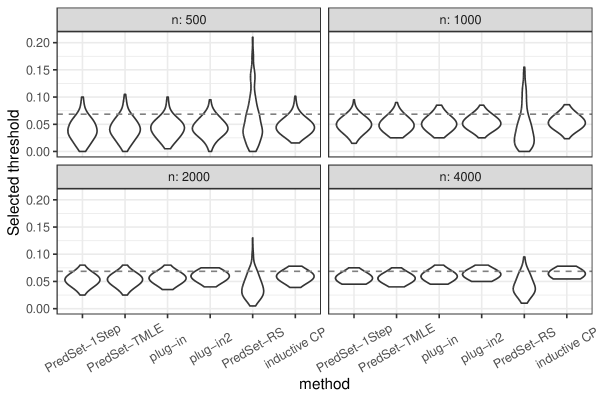
Figure S4: Violin plot of the sampling distribution of the selected threshold $\hat{\tau}_{n}$ in the moderate-to-high dimensional sparse setting. The gray horizontal dashed line is the true optimal threshold $\tau_{0}$.

As shown in Figure S4 in the Supplemental Material, the distribution of the threshold selected by PredSet-RS has a much wider spread than PredSet-1Step and PredSet-TMLE. We therefore recommend PredSet-1Step and PredSet-TMLE rather than PredSet-RS, although all these methods appear to produce APAC prediction sets.

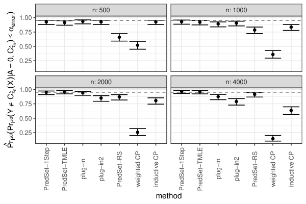
Figure 5: Empirical proportion of simulations where the estimated coverage error $\widehat{\mathrm{Pr}}_{P^{0}}(Y\notin C_{\hat{\tau}_{n}}(X)\mid A=0,C_{\hat{\tau}_{n}})$ does not exceed $\alpha_{\mathrm{error}}$, along with a 95% Wilson score confidence interval, in the moderate-to-high dimensional sparse setting. The gray horizontal dashed line is the desired confidence level $1-\alpha_{\mathrm{conf}}$.

5.2 Low dimensional setting

The data-generating mechanism is similar to the previous simulation. We still generate $A$ from a $\mathrm{Bernoulli}(0.5)$ random variable. We generate a three-dimensional covariate from a trivariate normal distribution:

$$X\mid A=a\sim\mathrm{N}\left(\begin{bmatrix}0\\ 0\\ 0\end{bmatrix},\begin{bmatrix}1&0.2&-0.2\\ 0.2&1&0.2\\ -0.2&0.2&1\end{bmatrix}\times\left(\frac{1}{2}\right)^{1-a}\right).$$

The outcome $Y$ also has three labels $\{0,1,2\}$ and is generated according to the distribution implied by the following two equations:

$$\frac{{\mathrm{Pr}}(Y=1\mid X=x)}{{\mathrm{Pr}}(Y=0\mid X=x)} =\exp(1.4x_{1}+1.5x_{2}-1.5x_{3}+0.3(1-x_{1})^{2}+0.015x_{2}x_{3}),$$

$$\frac{{\mathrm{Pr}}(Y=2\mid X=x)}{{\mathrm{Pr}}(Y=0\mid X=x)} =\exp(-0.1-1.3x_{1}-2.2x_{2}+0.5x_{3}+0.5(1-x_{2})^{2}+0.03x_{1}x_{3}).$$

The scoring function is determined by the following three equations, valid for all $x$: $s(x,0)+s(x,1)+s(x,2)=1$,

$$\frac{s(x,1)}{s(x,0)}=\exp(0.02+1.2x_{1}+1.91x_{2}-1.6x_{3}),\quad\text{and}\quad\frac{s(x,2)}{s(x,0)}=\exp(-0.03-1.5x_{1}-2.4x_{2}+0.3x_{3}).$$

Unlike in the previous simulation where $g_{0}$ follows a logistic regression model, here neither $g_{0}$ nor $\mathcal{E}_{0,\tau}$ follows a parametric model that is correctly specified by an algorithm in the library of Super Learner due to interaction terms in the distribution of $Y\mid X$ and quadratic terms in the logit of $w_{0}$. The only exceptions are that $\mathcal{E}_{0,\tau}$ follows a logistic regression model with an infinite slope for an extremely large or small threshold $\tau$. Thus, we do not expect our nuisance function estimators to generally converge at the parametric root-$n$ rate.

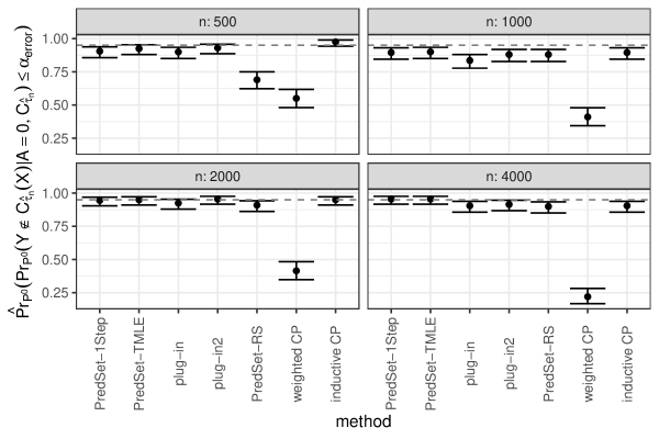
Figure S5: Empirical proportion of simulations where the estimated coverage error $\widehat{\mathrm{Pr}}_{P^{0}}(Y\notin C_{\hat{\tau}_{n}}(X)\mid A=0,C_{\hat{\tau}_{n}})$ does not exceed $\alpha_{\mathrm{error}}$, along with a 95% Wilson score confidence interval, in the low dimensional setting. The gray horizontal dashed line is the desired confidence level $1-\alpha_{\mathrm{conf}}$.

The simulation results are presented in Figures S5 and S6 in the Supplemental Material. The performance of the methods is similar to the moderate-to-high dimensional sparse setting.

5.3 Low dimensional setting without covariate shift

The data-generating mechanism is identical to the previous simulation, except that

$$X\mid A=a\sim\mathrm{N}\left(\begin{bmatrix}0\\ 0\\ 0\end{bmatrix},\begin{bmatrix}1&0.2&-0.2\\ 0.2&1&0.2\\ -0.2&0.2&1\end{bmatrix}\right).$$

In other words, covariate shift is not present.

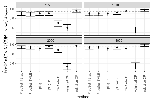
Figure S7: Empirical proportion of simulations where the estimated coverage error $\widehat{\mathrm{Pr}}_{P^{0}}(Y\notin C_{\hat{\tau}_{n}}(X)\mid A=0,C_{\hat{\tau}_{n}})$ does not exceed $\alpha_{\mathrm{error}}$, along with a 95% Wilson score confidence interval in the low dimensional setting without covariate shift. The gray horizontal dashed line is the desired confidence level $1-\alpha_{\mathrm{conf}}$.

The simulation results are presented in Figures S7 and S8 in the Supplemental Material. Inductive CP appears to perform the best for all sample sizes. This is not surprising, because inductive CP has a finite sample PAC guarantee in the no-covariate-shift setting. Our proposed methods PredSet-1Step and PredSet-TMLE also appear to be approximately PAC when the sample size is moderate to large ($n\geq 2000$). The performance of our proposed methods appears to be comparable to that of inductive CP, even under no covariate shift. The performance of the other two methods—plug-in and PredSet-RS—is similar to the previous simulation.

We therefore conclude from our simulations that, when the sample size is reasonably large, our proposed methods PredSet-1Step and PredSet-TMLE empirically output approximately PAC prediction sets regardless of whether covariate shift is present or not. Even when no covariate shift is present, in which case inductive CP has a finite sample PAC guarantee, the performance of our methods is empirically comparable with inductive CP. Our proposed methods can be applied as a default method if the user suspects—but may be unsure—that covariate shift is present, and does not know the likelihood ratio $w_{0}$ of the shift.

6 Analysis of HIV risk prediction data in South Africa

We illustrate our methods with a data set concerning HIV risk prediction in a South African cohort study. Specifically, we use data from a large population-based prospective cohort study in KwaZulu-Natal, South Africa which was collected and analyzed by Tanser et al. (2013) to evaluate the causal effect of community coverage of antiretroviral HIV treatment on community-level HIV incidence. The study followed a total of 16,667 individuals who were HIV-uninfected at baseline in order to observe individual HIV seroconversions over the period 2004 to 2011. In the present analysis, we aim to predict HIV seroconversion status over the follow-up period, for a target population of individuals living in a peri-urban community, using urban and rural communities as a source population.

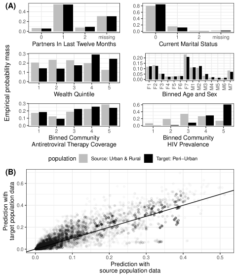
Figure S1: (A) Covariate distributions in the two populations of the data concerning HIV risk prediction in a South African cohort. A severe shift in community HIV prevalence and a moderate shift in wealth are present. (B) Outcome predictions for the entire data set with the predictors trained on the source population data and target population data, respectively, via Super Learner VanderLaan2007 with gradient boosting Friedman2001,Friedman2002,Mason1999,Mason2000 included in the library. The straight line $y=x$ represents identical predictions. Using data from the two populations, we obtain similar predictions for the entire data set, suggesting that the outcome distributions given covariates may be similar in the two populations.

Although the outcome is in fact available in both source and target samples, we deliberately treat the outcome in the target population as missing when constructing prediction sets, and then use the observed outcome in the target population to evaluate empirical coverage of prediction sets. There are 12385 and 5136 participants from source and target populations, respectively. All participants are treated as independent draws from their corresponding populations. The covariates used to predict the outcome are the followings: (i) binned number partners in the past 12 months, (ii) current marital status, (iii) wealth quintile, (iv) binned age and sex, (v) binned community antiretroviral therapy (ART) coverage, and (vi) binned community HIV prelevance. For covariates that are time-varying, we use the last observed value as the covariate. All covariates are treated as categorical variables in the analysis. Missing data for each covariate is treated as a separate category, which is equivalent to the missing-indicator method (Groenwold et al., 2012). Covariate distributions are presented in Figure S1 in the Supplemental Material. We also perform Fisher’s exact test via a Monte Carlo approximation with 2000 runs to test the equality of covariate distributions in the two populations, and we observe evidence of shift in covariate distribution with a p-value$<0.001$.

For illustration, in this analysis, we create a severe shift on a covariate that we believe to be strongly related to the outcome. In the target population, we only include individuals with community ART coverage below 15% (binned community ART coverage being 1 or 2 in Figure S1 in the Supplemental Material). In other words, we set the target population to be the population in the peri-urban communities with ART coverage below 15%, this sub-population maybe of particular public health policy interest as likely to carry most of the burden of incident HIV cases. We present the analysis results for the full data analysis (target population being peri-urban communities) in Section S6 in the Supplemental Material. In this subset of the data, there are 1418 participants from the target population.

We randomly select 10967 participants from the source population to train the scoring function $s$. We use Super Learner (van der Laan et al., 2007), with the same setup as in the simulations, to train a classifier of the outcome on this subsample, which is used as the scoring function $s$. We then construct prediction sets using the rest of the sample consisting of 1418 participants from each of the source and the target populations. The target PAC criterion has miscoverage level $\alpha_{\mathrm{error}}=0.05$ and confidence level $1-\alpha_{\mathrm{conf}}=0.95$. The methods we apply are a subset of the methods investigated in the simulations: PredSet-1Step, PredSet-TMLE, and inductive CP (Papadopoulos et al., 2002; Vovk, 2013; Park et al., 2021), which ignores covariate shift. The tuning parameters of these methods, such as the number of folds and the algorithm to estimate nuisance functions, are identical to those in the simulations.

The empirical coverage of the above methods in the sample from the target population is presented in Table 1. The empirical coverage of both PredSet-1Step and PredSet-TMLE is close to the target coverage level $1-\alpha_{\mathrm{error}}=95\%$, with the 95% confidence interval containing $1-\alpha_{\mathrm{error}}$. In constrast, the empirical coverage of inductive CP is lower than the target coverage level. Thus, properly accounting for covariate shift as in PredSet-1Step and PredSet-TMLE is crucial for achieving the PAC property in the “covariate shifted” target population in this subset of the data.

Table 1: Empirical coverage of prediction sets, 95% Wilson score confidence interval for coverage, and selected thresholds in the synthetic sample from the target population in the South Africa HIV trial data. The target coverage is at least $1-\alpha_{\mathrm{error}}=95\%$, with probability 95% over the training data.

Method	Empirical coverage	Coverage CI	Selected threshold $\hat{\tau}_{n}$
PredSet-1Step	95.98%	94.83%–96.89%	0.095
PredSet-TMLE	95.42%	94.20%–96.39%	0.100
Inductive Conformal Prediction	91.89%	90.35%–93.20%	0.195

7 Conclusion

There has been extensive literature on (i) constructing prediction sets based on fitted machine learning models, and (ii) supervised learning under covariate shift. In this work, we study the intersection of these two problems in the challenging setting where the covariate shift needs to be estimated. We propose a distribution-free method, PredSet-1Step, to construct asymptotically probably approximately correct (APAC) prediction sets under unknown covariate shift. PredSet-1Step may also be used to construct asymptotically risk controlling prediction sets (ARCPS) with a slight modification. Our method is flexible, taking as input an arbitrary given scoring function, produced by essentially any statistical or machine learning method.

We use semiparametric efficiency theory when constructing prediction sets to obtain root-$n$ convergence of the true miscoverage corresponding to the selected prediction sets, even if the estimators of the nuisance functions may converge slower than root-$n$. Our theoretical analysis of PredSet-1Step relies on a novel result on the convergence of Wald confidence intervals based on general asymptotically linear estimators, which is a technical tool of independent interest. We illustrate that our method has good coverage in a number of experiments and by analyzing a data set concerning HIV risk prediction in a South African cohort. In experiments without covariate shift, PredSet-1Step performs similarly to inductive CP, which has finite-sample PAC properties. Thus, PredSet-1Step may be used in the common scenario if the user suspects—but may not be certain—that covariate shift is present, and does not know the form of the shift.

One interesting open question is the asymptotic behavior of our selected threshold compared to the true optimal threshold. Our simulation results (Figures S4, S6 and S8 in the Supplemental Material) suggest that our selected threshold might converge in probability to the true optimal threshold. Our selected threshold also appears to have a vanishing negative bias that ensures the desired confidence level. Theoretical analysis is in need to confirm these conjectures.

Supplementary Material for “Prediction Sets
Adaptive to Unknown Covariate Shift”

This Supplementary Material is organized as follows. In Section S1, we describe another procedure, PredSet-RS, to construct APAC prediction sets, as well as its theoretical properties. We describe PredSet-TMLE and present its theoretical results in Section S2. We describe how to modify PredSet-1Step and PredSet-TMLE to construct asymptotically risk-controlling prediction sets in Section S3. We discuss double robustness of PredSet-1Step in Section S4. In Section S5, we illustrate that the convergence in supremum required by Condition 6 may be plausible with an example of nonparametric regression. In Section S6, we present analysis results of the full HIV risk prediction data in South Africa. We present proof of our theoretical results in Section S7. We finally discuss the difference between PAC guarantee (conditional validity) and marginal coverage guarantee (marginal validity), which is typically provided in conformal prediction methods, in Section S8. We discuss the connection between covariate shfit and causal inference in Section S9. We review the literature on confidence interval coverage based on efficient estimators involving nuisance function estimation in Section S10. We put supplemental figures at the end of this Supplemental Material.

We first introduce a few more functions for ease of presentation in the rest of this Supplemental Material. For each function $w:\mathcal{X}\mapsto[0,\infty)$, let $\Pi_{P}(w):={\mathbb{E}}_{P}[w(X)\mid A=1]=\int w(x)P_{X\mid 1}({\mathrm{d}}x)$. We note that $\Pi_{P}(w_{P})=\int 1{\mathrm{d}}P_{X\mid 0}=1$. For each $\tau\in\bar{\real}$, with $o:=(a,x,y)$, we define the following functions:

$$D^{\mathrm{Gcomp}}_{\tau}(P,\mathcal{E},g,\gamma,\pi):o \mapsto\frac{a}{\gamma_{P}}\mathscr{W}(g,\gamma)(x)\left\{Z_{\tau}(x,y)-\mathcal{E}_{P,\tau}(x)\right\}+\frac{1-a}{1-\gamma_{P}}[\mathcal{E}_{P,\tau}(x)-\Psi^{\mathrm{Gcomp}}_{\tau}(P)],$$ (S1)

$$\tilde{D}(\mathcal{E},g,\gamma,\pi):o \mapsto\mathcal{E}(x)\left\{-\frac{a}{\gamma}\frac{\mathscr{W}(g,\gamma)(x)}{\pi}+\frac{1-a}{1-\gamma}\right\}$$ (S2)

$$D^{\mathrm{weight}}_{\tau}(P,\mathcal{E},g,\gamma,\pi):o \mapsto\frac{a}{\gamma_{P}}\left\{\frac{\mathscr{W}(g,\gamma)(x)}{\Pi_{P}(\mathscr{W}(g,\gamma))}Z_{\tau}(x,y)-\Psi^{\mathrm{weight}}_{\tau}(P)\right\}$$

$$+\Psi^{\mathrm{weight}}_{\tau}(P)\frac{a-\gamma_{P}}{\gamma_{P}(1-\gamma_{P})}+\tilde{D}(\mathcal{E},g,\gamma,\pi).$$

Though seemingly different, $D^{\mathrm{Gcomp}}_{\tau}(P,\mathcal{E}_{P,\tau},g_{P},\gamma_{P},1)$ and $D^{\mathrm{weight}}_{\tau}(P,\mathcal{E}_{P,\tau},g_{P},\gamma_{P},1)$ are identical to $D_{\tau}(P,g_{P},\gamma_{P})$. In our definitions, the arguments $\mathcal{E}$ and $\pi$ of $D^{\mathrm{Gcomp}}_{\tau}$ are unused. We keep these unused arguments in our notation to keep the arguments of $D^{\mathrm{Gcomp}}_{\tau}$ and $D^{\mathrm{weight}}_{\tau}$ consistent. We also refer to $D^{\mathrm{Gcomp}}_{\tau}(P,\mathcal{E}_{P,\tau},g_{P},\gamma_{P},1)$ and $D^{\mathrm{weight}}_{\tau}(P,\mathcal{E}_{P,\tau},g_{P},\gamma_{P},1)$ as $D_{\tau}(P,\mathcal{E}_{P,\tau},g_{P},\gamma_{P},1)$ when we need not distinguish their mathematical expressions, where we have redefined

$$D_{\tau}(P,\mathcal{E}_{P,\tau},g_{P},\gamma_{P},1):o \mapsto\frac{a}{\gamma_{P}}\mathscr{W}(g_{P},\gamma_{P})(x)\left\{Z_{\tau}(x,y)-\mathcal{E}_{P,\tau}(x)\right\}+\frac{1-a}{1-\gamma_{P}}[\mathcal{E}_{P,\tau}(x)-\Psi_{\tau}(P)]$$ (S3)

with a slight abuse of notations. With these definitions, $D_{\tau}$ in (12) is essentially $D^{\mathrm{Gcomp}}_{\tau}$ in (S1).

We introduce two versions of gradient functions $D^{\mathrm{Gcomp}}_{\tau}$ and $D^{\mathrm{weight}}_{\tau}$ because they are used in estimation of $\Psi_{\tau}(P^{0})$ with the two identifying functionals $\Psi^{\mathrm{Gcomp}}_{\tau}$ and $\Psi^{\mathrm{weight}}_{\tau}$ respectively. For the main method we propose in Section 4.1, namely PredSet-1Step, $D^{\mathrm{Gcomp}}_{\tau}$ is used and thus we use a simplified notation in the main text for conciseness; for another method we propose in Section S1, namely PredSet-RS, $D^{\mathrm{weight}}_{\tau}$ is used.

S1 PredSet-RS

In this section, we describe another procedure, PredSet-RS, to construct APAC prediction sets based on rejection sampling along with its main theoretical properties. This procedure is an extension of the method in park2021pac. We first split the data into training and testing data with observation index sets $I_{\mathrm{train}}$ and $I_{\mathrm{test}}$, respectively. Throughout this paper, we assume that the training data set size is

$$|I_{\mathrm{train}}|=n\xi+{\mathrm{O}}(n^{-1})$$ (S4)

for a constant $\xi\in(0,1)$, which holds if the size of both training and testing data sets are approximately $n/2$. Since we treat the scoring rule $s$ as fixed, these data sets are independent of the original training data where $s$ was learned.

We first estimate the likelihood ratio $w_{0}$ based on $I_{\mathrm{train}}$. Then we generate a sample of independent $(X,Y)$-s, with a distribution close to the target population, by applying rejection sampling with the estimated likelihood ratio as the weight to the test data from the source population. Next, for each candidate $\tau\in\mathcal{T}_{n}$, we use the corresponding Bernoulli sample of $Z_{\tau}$ from the data obtained via rejection sampling to estimate $\Psi_{\tau}(P^{0})$. In particular, we apply a one-step correction to the sample proportion to account for the estimation of $w_{0}$ when estimating $\Psi_{\tau}(P^{0})$ and then calculate a Wald CUB. We finally use the approximate CUB to select thresholds similarly to Section 4. We next describe this procedure in more detail.

S1.1 Rejection sampling from an approximation to the target population

Let $\hat{g}_{n}^{\mathrm{train}}$, $\hat{\mathcal{E}}_{n,\tau}^{\mathrm{train}}$ and $\hat{\gamma}_{n}^{\mathrm{train}}$ be estimators of $g_{0}$, $\mathcal{E}_{0,\tau}$ and $\gamma_{0}$, respectively, obtained using the training data $I_{\mathrm{train}}$. Let $\breve{P}^{n}$ be an oracle distribution estimator (i.e., a distribution with some components that are not based on empirically observed quantities, but rather based on population quantities) with the following components:

1. marginal distribution of $A$ being $P^{0}_{A}$;

2. conditional distribution of $X\mid A=1$ being $P^{0}_{X\mid 1}$;

3. conditional distribution of $Y\mid X=x,A=1$ being $P^{0}_{Y\mid x}$;

4. likelihood ratio (with normalizing constant):

   $$\mathscr{W}(\hat{g}_{n}^{\mathrm{train}},\hat{\gamma}_{n}^{\mathrm{train}})/\Pi_{P^{0}}(\mathscr{W}(\hat{g}_{n}^{\mathrm{train}},\hat{\gamma}_{n}^{\mathrm{train}})).$$ (S5)

We aim at drawing i.i.d. samples from $\breve{P}^{n}$, based on which we may construct a CUB for $\Psi_{\tau}(\breve{P}^{n})$ as an approximate CUB for $\Psi_{\tau}(P^{0})$. We make the following assumption so that rejection sampling may be conducted.

Condition S1 (Known bound on likelihood ratio estimator).

There is a known constant $\hat{B}\in[1,\infty)$ such that, for some non-negative sequence $(\breve{q}_{n})_{n\geqslant 1}$ tending to zero, $\sup_{x\in\mathcal{X}}\mathscr{W}(\hat{g}_{n}^{\mathrm{train}},\hat{\gamma}_{n}^{\mathrm{train}})(x)\leq\hat{B}$ with probability $1-\breve{q}_{n}$.

The known constant $\hat{B}$ in Condition S1 may differ from the constant $B$ in Condition 4. Since $\sup_{x\in\mathcal{X}}w_{0}(x)\geq{\mathbb{E}}_{P^{0}}[w_{0}(X)\mid A=1]=1$, we have assumed without loss of generality that $\hat{B}\geq 1$. In practice, to specify $\hat{B}$, it is possible for the user to investigate all $g_{n}^{\mathrm{train}}(X_{i})$, for $i\in I_{\mathrm{test}}$, and choose $\hat{B}$ to be $\max_{i\in I_{\mathrm{test}}}\mathscr{W}(g_{n}^{\mathrm{train}},\gamma_{n}^{\mathrm{train}})(X_{i})$ or a number greater by, for example, 30%. Another possible option is to prespecify a lower bound $\hat{\delta}\in(0,1)$ for $g_{n}^{\mathrm{train}}$ and choose $\hat{B}$ to be $\frac{1-\hat{\delta}}{\hat{\delta}}\frac{\gamma_{n}^{\mathrm{train}}}{1-\gamma_{n}^{\mathrm{train}}}$ or a number greater by, for example, 30%. These are heuristic ad hoc approaches to specify $\hat{B}$ that lack strong theoretical support. As discussed after we introduced Condition 5 in Section 4.1, for suitably chosen $\hat{B}$, we can often expect $\breve{q}_{n}$ to vanish at an exponential rate.

We next describe the rejection sampling procedure vonNeumann1951. We generate exogenous random variables

$$\zeta_{i}\overset{i.i.d.}{\sim}\mathrm{Unif}(0,1),$$ (S6)

for $i\in I_{\mathrm{test}}$, and we output the sample

$$S_{n}:=\{O_{i}:A_{i}=1,\zeta_{i}\leq\mathscr{W}(\hat{g}_{n}^{\mathrm{train}},\hat{\gamma}_{n}^{\mathrm{train}})(X_{i})/\hat{B},i\in I_{\mathrm{test}}\}.$$

We use $J_{n}$ to denote the set of the indices of observations in $S_{n}$.

Since $\mathscr{W}(\hat{g}_{n}^{\mathrm{train}},\hat{\gamma}_{n}^{\mathrm{train}})$ might not be a valid likelihood ratio in the sense that $\Pi_{P^{0}}(\mathscr{W}(\hat{g}_{n}^{\mathrm{train}},\hat{\gamma}_{n}^{\mathrm{train}}))$ might not equal unity, our rejection sampling procedure is different from the ordinary one where a valid likelihood ratio is known. However, we still have the following result that is similar to the properties of the usual rejection sampling.

Theorem S1 (Properties of rejection sampling).

Conditional on the training data and the event $\sup_{x\in\mathcal{X}}\mathscr{W}(\hat{g}_{n}^{\mathrm{train}},\hat{\gamma}_{n}^{\mathrm{train}})(x)\leq\hat{B}$, where $\hat{g}_{n}^{\mathrm{train}}$ and $\hat{\gamma}_{n}^{\mathrm{train}}$ are estimators $g_{0}$ and $\gamma_{0}$ from the beginning of Section S1.1 respectively, $\mathscr{W}$ is defined in (9), and $\hat{B}$ is from (S1), the accepted covariate-outcome pairs $\{(X_{i},Y_{i}):i\in J_{n}\}$ are an i.i.d. sample drawn from $(X,Y)\mid A=0$ under the approximation $\breve{P}^{n}$ to the target population defined at the beginning of Section S1.1. In addition, for all $i\in I_{\mathrm{test}}$, the acceptance probability equals (with $\zeta_{i}$ defined in (S6), and the normalizing factor $\Pi_{P^{0}}(\mathscr{W}(\hat{g}_{n}^{\mathrm{train}},\hat{\gamma}_{n}^{\mathrm{train}}))$ from (S5))

$${\mathrm{Pr}}_{P^{0}}(A_{i}=1,\zeta_{i}\leq\mathscr{W}(\hat{g}_{n}^{\mathrm{train}},\hat{\gamma}_{n}^{\mathrm{train}})(X_{i})/\hat{B})=\gamma_{0}\Pi_{P^{0}}(\mathscr{W}(\hat{g}_{n}^{\mathrm{train}},\hat{\gamma}_{n}^{\mathrm{train}}))/\hat{B}.$$

The proof of Theorem S1 can be found in Section S7.5 in the Supplemental Material. As in ordinary rejection sampling, the acceptance probability is inversely proportional to the known bound $\hat{B}$ on the likelihood ratio. Therefore, if $\hat{B}$ is large, for example, due to severe covariate shift, rejection sampling might output a small sample, which may lead to significant inefficiency and inaccuracy in small to moderate samples for PredSet-RS. In contrast, PredSet-1Step might not suffer as much from a severe covariate shift. This heuristic is supported by our later simulation results.

S1.2 One-step correction and standard error

Since $\{(X_{i},Y_{i}):i\in J_{n}\}$ are an i.i.d. sample drawn from $(X,Y)\mid A=0$ under $\breve{P}^{n}$, it is not difficult to see that $\sum_{i\in J_{n}}Z_{\tau}(X_{i},Y_{i})$ is distributed as $\mathrm{Binom}(|J_{n}|,\Psi_{\tau}(\breve{P}^{n}))$ conditional on $\mathscr{W}(\hat{g}_{n}^{\mathrm{train}},\hat{\gamma}_{n}^{\mathrm{train}})$ and $|J_{n}|$. It might be tempting to use $\sum_{i\in J_{n}}Z_{\tau}(X_{i},Y_{i})/|J_{n}|$ as an estimator of $\Psi_{\tau}(P^{0})$, and subsequently to use existing methods to construct binomial proportion CUBs, such as the Clopper-Pearson (CP) CUB Clopper1934 or the Wilson score CUB Wilson1927, to construct a CUB for $\Psi_{\tau}(\breve{P}^{n})$, which serves as an approximate CUB for $\Psi_{\tau}(P^{0})$.

However, this naïve approach does not account for the estimation error of the likelihood ratio $w_{0}$ used in rejection sampling, typically of a rate slower than $n^{-1/2}$ under a nonparametric model. In addition, the standard error used in ordinary binomial proportion CUBs is also invalid with an estimated likelihood ratio, even if a correction is applied to obtain root-$n$-consistency. These issues may invalidate the APAC criterion.

We next describe a one-step correction to $\sum_{i\in J_{n}}Z_{\tau}(X_{i},Y_{i})/|J_{n}|$, and its asymptotic properties. Recall that $\hat{\mathcal{E}}_{n,\tau}^{\mathrm{train}}$ is an estimator of $\mathcal{E}_{0,\tau}$ obtained using training data $I_{\mathrm{train}}$. Let

$$\hat{\pi}_{n}:=\frac{\sum_{i\in I_{\mathrm{test}}}A_{i}\mathscr{W}(\hat{g}_{n}^{\mathrm{train}},\hat{\gamma}_{n}^{\mathrm{train}})(X_{i})}{\sum_{i\in I_{\mathrm{test}}}A_{i}}$$ (S7)

be an estimator of $\Pi_{P^{0}}(\mathscr{W}(\hat{g}_{n}^{\mathrm{train}},\hat{\gamma}_{n}^{\mathrm{train}}))$ and

$$\breve{\psi}_{n,\tau} :=\frac{\sum_{i\in J_{n}}Z_{\tau}(X_{i},Y_{i})}{|J_{n}|}+\frac{1}{|I_{\mathrm{test}}|}\sum_{i\in I_{\mathrm{test}}}\tilde{D}(\hat{\mathcal{E}}_{n,\tau}^{\mathrm{train}},\hat{g}_{n}^{\mathrm{train}},\hat{\gamma}_{n}^{\mathrm{train}},\hat{\pi}_{n})(O_{i})$$ (S8)

$$=\frac{\sum_{i\in J_{n}}Z_{\tau}(X_{i},Y_{i})}{|J_{n}|}+\frac{1}{|I_{\mathrm{test}}|}\sum_{i\in I_{\mathrm{test}}}\hat{\mathcal{E}}_{n,\tau}^{\mathrm{train}}(X_{i})\left[-\frac{A_{i}}{\hat{\gamma}_{n}^{\mathrm{train}}}\frac{\mathscr{W}(\hat{g}_{n}^{\mathrm{train}},\hat{\gamma}_{n}^{\mathrm{train}})(X_{i})}{\hat{\pi}_{n}}+\frac{1-A_{i}}{1-\hat{\gamma}_{n}^{\mathrm{train}}}\right].$$

We will show that this corrected estimator $\breve{\psi}_{n,\tau}$ based on the sample proportion $\sum_{i\in J_{n}}Z_{\tau}(X_{i},Y_{i})/|J_{n}|$ is asymptotically normal under certain conditions. We next present an additional condition that is similar to Condition 6, and a theorem on the theoretical properties of $\breve{\psi}_{n,\tau}$.

Condition S2 (Sufficient rates for nuisance estimators).

The following conditions hold.

$${\mathbb{E}}_{P^{0}}\sup_{\tau\in\mathcal{T}_{n}}\|\hat{\mathcal{E}}_{n,\tau}^{\mathrm{train}}-\mathcal{E}_{0,\tau}\|_{P^{0}_{X\mid 0},2}={\mathrm{o}}(1),\qquad{\mathbb{E}}_{P^{0}}\left\|\mathscr{W}(\hat{g}_{n}^{\mathrm{train}},\hat{\gamma}_{n}^{\mathrm{train}})-\mathscr{W}(g_{0},\gamma_{0})\right\|_{P^{0}_{X\mid 0},2}={\mathrm{o}}(1),$$

$${\mathbb{E}}_{P^{0}}\sup_{\tau\in\mathcal{T}_{n}}\int\left|\left\{\frac{\mathscr{W}(\hat{g}_{n}^{\mathrm{train}},\hat{\gamma}_{n}^{\mathrm{train}})(x)}{\Pi_{P^{0}}(\mathscr{W}(\hat{g}_{n}^{\mathrm{train}},\hat{\gamma}_{n}^{\mathrm{train}}))}-\mathscr{W}(g_{0},\gamma_{0})(x)\right\}\left\{\hat{\mathcal{E}}_{n,\tau}^{\mathrm{train}}(x)-\mathcal{E}_{0,\tau}(x)\right\}\right|P^{0}_{X\mid 1}({\mathrm{d}}x)={\mathrm{o}}(n^{-1/2}).$$

The difference between Condition 6 and Condition S2 is that Condition S2 mainly requires a convergence rate on the normalized likelihood ratio estimator in the product term while Condition 6 mainly requires a convergence rate on the odds ratio estimator. Since the likelihood ratio estimator and the odds ratio estimator differ by a factor that converges to the truth at root-$n$ rate (see Section 3.1), we do not expect these two conditions to be substantially different in practice. Strictly speaking, the required convergence of the unnormalized estimator $\mathscr{W}(\hat{g}_{n}^{\mathrm{train}},\hat{\gamma}_{n}^{\mathrm{train}})$ to $\mathscr{W}(g_{0},\gamma_{0})$ in Condition S2 may be relaxed to convergence to a constant multiple of $\mathscr{W}(g_{0},\gamma_{0})$. We do not take this route, since it is unclear how this relaxed condition may arise in practice.

Theorem S2 (Asymptotic normality of one-step corrected estimator $\breve{\psi}_{n,\tau}$).

Under Conditions 1–4, S1 and S2, with the coverage error $\Psi_{\tau}(P^{0})$, $\gamma_{0},g_{0}$ from (8), $\hat{B}$ from (S1), $\zeta_{i}$ from (S6), $w_{0}$ from Condition 3, $\mathcal{E}_{0,\tau}$ from (6), and $\tilde{D}$ from (S2), defining

$$\Gamma_{n,\tau} :=\frac{1}{|I_{\mathrm{train}}|}\sum_{i\in I_{\mathrm{train}}}\frac{A_{i}-\gamma_{0}}{\gamma_{0}(1-\gamma_{0})}\Psi_{\tau}(P^{0})$$

$$\qquad+\frac{1}{|I_{\mathrm{test}}|}\sum_{i\in I_{\mathrm{test}}}\Bigg{\{}\hat{B}\frac{A_{i}}{\gamma_{0}}{\mathbbm{1}}(\zeta_{i}\leq w_{0}(X_{i})/\hat{B})[Z_{\tau}(X_{i},Y_{i})-\Psi_{\tau}(P^{0})]$$

$$\qquad\qquad+\frac{A_{i}[w_{0}(X_{i})-1]}{\gamma_{0}}\Psi_{\tau}(P^{0})+\tilde{D}(\mathcal{E}_{0,\tau},g_{0},\gamma_{0},1)(O_{i})\Bigg{\}},$$

for the one-step corrected estimator $\breve{\psi}_{n,\tau}$ based on rejection sampling from (S8), it holds that

$$\sup_{\tau\in\mathcal{T}_{n}}\left|\breve{\psi}_{n,\tau}-\Psi_{\tau}(P^{0})-\Gamma_{n,\tau}\right|={\mathrm{o}}_{p}(n^{-1/2}).$$

The proof of Theorem S2 can be found in Section S7.6 in the Supplemental Material.

Since, for each $\tau\in\mathcal{T}_{n}$, $\Gamma_{n,\tau}$ is the sum of two independent sample means with mean zero, we have that both $\sqrt{n}\Gamma_{n,\tau}$ and $\sqrt{n}(\breve{\psi}_{n,\tau}-\Psi_{\tau}(P^{0}))$ converge in distribution to $\mathrm{N}(0,\varsigma_{0}^{2})$, where

$$\begin{split}\varsigma_{0,\tau}^{2}&:=\xi^{-1}{\mathbb{E}}_{P^{0}}\left[\frac{(A-\gamma_{0})^{2}}{\gamma_{0}^{2}(1-\gamma_{0})^{2}}\Psi_{\tau}(P^{0})^{2}\right]\\ &\quad+(1-\xi)^{-1}{\mathbb{E}}_{P^{0}}\Bigg{[}\Bigg{\{}\hat{B}\frac{A}{\gamma_{0}}{\mathbbm{1}}(\zeta\leq w_{0}(X)/\hat{B})[Z_{\tau}(X,Y)-\Psi_{\tau}(P^{0})]\\ &\qquad\qquad+\frac{A[w_{0}(X)-1]}{\gamma_{0}}\Psi_{\tau}(P^{0})+\tilde{D}(\mathcal{E}_{0,\tau},g_{0},\gamma_{0},1)(O)\Bigg{\}}^{2}\Bigg{]}.\end{split}$$ (S9)

A consistent estimator of the asymptotic variance of $\breve{\psi}_{n,\tau}$ is

$$\begin{split}\hat{\varsigma}_{n,\tau}^{2}&:=\frac{n}{|I_{\mathrm{train}}|}\frac{1}{|I_{\mathrm{train}}|}\sum_{i\in I_{\mathrm{train}}}\frac{(A_{i}-\hat{\gamma}_{n}^{\mathrm{train}})^{2}}{(\hat{\gamma}_{n}^{\mathrm{train}})^{2}(1-\hat{\gamma}_{n}^{\mathrm{train}})^{2}}\breve{\psi}_{n,\tau}^{2}\\ &\qquad+\frac{n}{|I_{\mathrm{test}}|}\frac{1}{|I_{\mathrm{test}}|}\sum_{i\in I_{\mathrm{test}}}\Bigg{\{}\hat{B}\frac{A_{i}}{\hat{\gamma}_{n}^{\mathrm{train}}}{\mathbbm{1}}(\zeta_{i}\leq\mathscr{W}(\hat{g}_{n}^{\mathrm{train}},\hat{\gamma}_{n}^{\mathrm{train}})(X_{i})/\hat{B})[Z_{\tau}(X_{i},Y_{i})-\breve{\psi}_{n,\tau}]\\ &\qquad\qquad+\frac{A_{i}[\mathcal{W}(\hat{g}_{n}^{\mathrm{train}},\hat{\gamma}_{n}^{\mathrm{train}})(X_{i})-1]}{\hat{\gamma}_{n}^{\mathrm{train}}}\breve{\psi}_{n,\tau}+\tilde{D}(\hat{\mathcal{E}}_{n,\tau}^{\mathrm{train}},\hat{g}_{n}^{\mathrm{train}},\hat{\gamma}_{n}^{\mathrm{train}},\hat{\pi}_{n})(O_{i})\Bigg{\}}^{2}.\end{split}$$ (S10)

We may then use the Wald CUB $\breve{\psi}_{n,\tau}+z_{\alpha_{\mathrm{conf}}}\hat{\varsigma}_{n,\tau}/\sqrt{n}$ as an asymptotically valid CUB for $\Psi_{\tau}(P^{0})$. Finally, similarly to PredSet-1Step, we let

$$\hat{\tau}^{\mathrm{RS}}_{n}:=\max\{\tau\in\mathcal{T}_{n}:\breve{\psi}_{n,\tau^{\prime}}+z_{\alpha_{\mathrm{conf}}}\hat{\varsigma}_{n,\tau^{\prime}}/\sqrt{n}<\alpha_{\mathrm{error}}\text{ for all }\tau^{\prime}\in\mathcal{T}_{n}\text{ such that }\tau^{\prime}\leq\tau\}.$$ (S11)

be the selected threshold based on rejection sampling. This step is also illustrated in Figure S2. We propose to use $C_{\hat{\tau}^{\mathrm{RS}}_{n}}$ as the prediction set.

We have the following result on the coverage of the Wald CUB and the APAC property of $C_{\hat{\tau}^{\mathrm{RS}}_{n}}$. Recall $\mathcal{T}^{\varepsilon}$ defined in Section 4.2.

Theorem S3.

Under Conditions 1–4, S1 and S2, for any fixed $\varepsilon>0$, with probability tending to one, for the one-step corrected estimator $\breve{\psi}_{n,\tau}$ of the coverage error $\Psi_{\tau}(P^{0})$ based on rejection sampling from (S8) and the variance estimator $\hat{\varsigma}_{n,\tau}^{2}$ from (S10), it holds that (with $\mathcal{T}^{\varepsilon}$ from (18)),

$$\sup_{\tau\in\mathcal{T}^{\varepsilon}}\left|{\mathrm{Pr}}_{P^{0}}(\Psi_{\tau}(P^{0})\leq\breve{\psi}_{n,\tau}+z_{\alpha_{\mathrm{conf}}}\hat{\varsigma}_{n,\tau}/\sqrt{n})-(1-\alpha_{\mathrm{conf}})\right|\lesssim\breve{\Delta}_{n,\varepsilon},$$

where with $\mathscr{W}$ from (9), $\hat{g}_{n}^{\mathrm{train}},\hat{\gamma}_{n}^{\mathrm{train}},\hat{\mathcal{E}}_{n,\tau}^{\mathrm{train}}$ from the beginning of Section S1.1, $g_{0},\gamma_{0}$ from (8), $\mathcal{E}_{0,\tau}$ from (6), the marginal distribution $P^{0}_{X\mid 1}$ of $X$ in the source population from Condition 3, probability $1-\breve{q}_{n}$ of $\hat{B}$ bounding the estimated likelihood ratio in Condition S1,

$$\begin{split}\breve{\Delta}_{n,\varepsilon}&:=n^{1/4}\varepsilon^{-1/4}\sup_{\tau\in\mathcal{T}_{n}}\left\{{\mathbb{E}}_{P^{0}}\left|\int\left(\frac{\mathscr{W}(\hat{g}_{n}^{\mathrm{train}},\hat{\gamma}_{n}^{\mathrm{train}})(x)}{\hat{\pi}_{n}}-\mathscr{W}(g_{0},\gamma_{0})(x)\right)\cdot(\hat{\mathcal{E}}_{n,\tau}^{\mathrm{train}}(x)-\mathcal{E}_{0,\tau}(x))P^{0}_{X\mid 1}({\mathrm{d}}x)\right|\right\}^{1/2}\\ &\quad+\breve{q}_{n}\end{split}$$ (S12)

converges to zero. In addition, under Condition 7, for all $\tau$ such that $\Psi_{\tau}(P^{0})=0$, it holds that ${\mathrm{Pr}}_{P^{0}}(\Psi_{\tau}(P^{0})\leq\breve{\psi}_{n,\tau}+z_{\alpha_{\mathrm{conf}}}\hat{\varsigma}_{n,\tau}/\sqrt{n})=1$ with probability tending to one.

Moreover, under Condition 8, it holds that

$${\mathrm{Pr}}_{P^{0}}(\Psi_{\hat{\tau}^{\mathrm{RS}}_{n}}(P^{0})\leq\alpha_{\mathrm{error}})\geq 1-\alpha_{\mathrm{conf}}-{\mathscr{C}}\breve{\Delta}_{n,\varepsilon}.$$ (S13)

In other words, the prediction set with threshold $\hat{\tau}^{\mathrm{RS}}_{n}$ is APAC.

The proof of Theorem S3 is similar to Theorem 5 and Corollary 1. A sketch can be found in Section S7.6 in the Supplemental Material.

A natural question is whether PredSet-1Step or PredSet-RS is preferred. Since $\hat{\pi}_{n}$ is consistent for unity, we expect the error of the confidence levels $\breve{\Delta}_{n,\varepsilon}$ and $\Delta_{n,\varepsilon}$ to be of comparable order. However, we have the following result on the superior accuracy of PredSet-1Step compared to PredSet-RS.

Theorem S4.

For any $\tau\in\mathcal{T}^{0}$, for the asymptotic variance $\sigma_{0,\tau}^{2}:={\mathbb{E}}_{P^{0}}[D_{\tau}(P^{0},\mathcal{E}_{0,\tau},g_{0},\gamma_{0},1)(O)^{2}]$ of the one-step corrected estimator $\hat{\psi}_{n,\tau}$ from (16) and the asymptotic variance $\varsigma_{0,\tau}^{2}$ from (S9) of the rejection sampling-based estimator $\breve{\psi}_{n,\tau}$ from (S8), it holds that $\sigma_{0,\tau}^{2}<\varsigma_{0,\tau}^{2}$.

This result shows that $\breve{\psi}_{n,\tau}$ is a less accurate estimator of $\Psi_{\tau}(P^{0})$ than $\hat{\psi}_{n,\tau}$, and thus has a wider two-sided Wald CI. Therefore, we expect the distribution of $\hat{\tau}^{\mathrm{RS}}_{n}$ to have a wider spread than that of $\hat{\tau}^{\mathrm{1Step}}_{n}$. Thus, PredSet-RS provides an overly conservative threshold more often than PredSet-1Step. The proof of Theorem S4 can be found in Section S7.6 in the Supplemental Material.

Remark 11.

In our procedure, it is possible to reverse the role of training and test data and obtain two approximate CUBs. In general, we may split the data into $V$ folds, split $\alpha_{\mathrm{conf}}$ into $\alpha_{\mathrm{conf}}=\sum_{v=1}^{V}\alpha_{\mathrm{conf}}^{v}$, treat the data in and out of each fold as testing and training data respectively, and obtain $V$ approximate $(1-\alpha_{\mathrm{conf}}^{v})$-level CUBs. We may then set the combined CUB to be the minimum of these CUBs, and the argument for Bonferroni correction Bonferroni1936,Dunn1961,Bland1995 implies that the confidence level of the combined CUB is at least $1-\alpha_{\mathrm{conf}}-{\mathscr{C}}\breve{\Delta}_{\varepsilon,n}$. However, it is well known that Bonferroni correction is conservative Bland1995,Bender1999,Moran2003, especially if $V$ is large, and hence we do not advocate for this approach. Other simple methods—for example, based on treating these $V$ CUBs as independent—might not apply, because the CUBs are constructed from the entire data and are thus dependent.

S1.3 Tuning parameters of PredSet-RS in simulations

In all simulations in Section 5, we split the data such that $|I_{\mathrm{train}}|=|I_{\mathrm{test}}|=n/2$. Nuisance functions $g_{0}$ and $\mathcal{E}_{0,\tau}$ are estimated with the identical method as in PredSet-1Step and PredSet-TMLE.

In the moderate-to-high dimensional setting, the maximum of the true likelihood ratio equals 4, and we set $\hat{B}$ in Condition S1 to be 8 for PredSet-RS. In the low dimensional settings (both with and without covariate shift), the true likelihood ratio is bounded by $2^{3/2}\approx 2.8$, and we set $\hat{B}$ to be a larger number 5.5. We chose these bounds to account for the estimation error in the likelihood ratio and the user’s a priori ignorance of a tight bound on the estimated likelihood ratio.

S2 Alternative to one-step correction: targeted minimum-loss based estimation (TMLE)

In this section, we present an alternative method PredSet-TMLE to PredSet-1Step as mentioned in Remark 8. When constructing asymptotically efficient estimators of $\Psi_{\tau}(P^{0})$, we may use cross-validated targeted minimum-loss based estimators (CV-TMLE) VanderLaan2006,VanderLaan2018. After splitting the data into $V$ folds as in Section 4, a CV-TMLE is constructed as in the following Algorithm S1.

Algorithm S1 CV-TMLE of coverage error $\Psi_{\tau}(P^{0})$ used in PredSet-TMLE

1:Obtain initial estimators $\hat{g}_{n}^{-v}$ and $\hat{\mathcal{E}}_{n,\tau}^{-v}$ of nuisance functions $g_{0}$ and $\mathcal{E}_{0,\tau}$ using the same procedure as Lines 1–4 in Algorithm 1.

2:for $\tau\in\mathcal{T}_{n}$ and $v\in[V]$ do $\triangleright$ (Obtain a TMLE for fold $v$ based on sample splitting)

3:     If $Z_{\tau}(X,Y)$ is not all zero or all one, perform logistic regression with outcome $Z_{\tau}(X,Y)$, offset $\operatorname{logit}\{\hat{\mathcal{E}}_{n,\tau}^{-v}(X)\}$, clever covariate $\mathscr{W}(\hat{g}_{n}^{-v},\hat{\gamma}_{n}^{v})(X)$, and no intercept; using data with $A=1$ in fold $v$. Set $\tilde{\mathcal{E}}_{n,\tau}^{v}$ to be the fitted mean model. Otherwise, when $\hat{\mathcal{E}}_{n,\tau}^{-v}$ is constant zero or one, we set $\tilde{\mathcal{E}}_{n,\tau}^{v}:=\mathcal{E}_{n,\tau}^{-v}$.

4:     Let $\tilde{P}_{\tau}^{n,v}$ be a distribution with the following components: (i) marginal distribution of $A$ being $P_{A}^{n,v}$, (ii) conditional distribution of $X\mid A=0$ being $P_{X\mid 0}^{n,v}$, (iii) distribution of $Z_{\tau}\mid X,A=1$ defined by $\tilde{\mathcal{E}}_{n,\tau}^{v}$, and (iv) likelihood ratio $\mathscr{W}(\hat{g}_{n}^{-v},\hat{\gamma}_{n}^{-v})$.

5:     Set

$$\tilde{\psi}_{n,\tau}^{v}:=\Psi^{\mathrm{Gcomp}}(\tilde{P}_{\tau}^{n,v})=\frac{\sum_{i\in I_{v}}(1-A_{i})\tilde{\mathcal{E}}_{n,\tau}^{v}(X_{i})}{\sum_{i\in I_{v}}(1-A_{i})}.$$

6:for $\tau\in\mathcal{T}_{n}$ do

7:     Obtain the CV-TMLE $\tilde{\psi}_{n,\tau}:=\frac{1}{n}\sum_{v=1}^{V}|I_{v}|\tilde{\psi}_{n,\tau}^{v}$.

We assume that Condition 7 holds for $\hat{\mathcal{E}}_{n,\tau}^{-v}$. It is then not hard to check that $\tilde{\psi}_{n,\tau}^{v}$ always lies in the interval $[0,1]$, the range known to contain $\Psi_{\tau}(P^{0})$, and thus so does $\tilde{\psi}_{n,\tau}$. This is different from the cross-fit one-step corrected estimator $\psi_{n,\tau}$ in (14), which may fall out of this known range, and hence $\tilde{\psi}_{n,\tau}$ may be preferable to $\hat{\psi}_{n,\tau}$.

However, the logistic regression procedure in Line 3 of Algorithm S1 may fail or be numerically unstable if, for some $i\in I_{v}$, $\hat{\mathcal{E}}_{n,\tau}^{-v}(X_{i})$ is equal or close to zero or one. This may happen when the threshold $\tau$ is too small or too large. In such cases, we may replace this logistic regression step with an ordinary least squares fit with the same setup, except that the offset is $\hat{\mathcal{E}}_{n,\tau}^{-v}(X)$ instead. The resulting targeted conditional coverage error estimator might fall out of the interval $[0,1]$, but the asymptotic behavior of the corresponding CV-TMLE remains the same. In our implementation, we use ordinary least-squares in Step 3 whenever a numerical issue, namely a warning or error, occurs in our implementation when running a logistic regression.

We estimate the asymptotic variance similarly to the way it is done in Section 4.2. Let

$$(\tilde{\sigma}_{n,\tau}^{v})^{2}:=\frac{1}{|I_{v}|}\sum_{i\in I_{v}}D^{\mathrm{Gcomp}}(\tilde{P}_{\tau}^{n,v},\tilde{\mathcal{E}}_{n,\tau}^{v},\hat{g}_{n}^{-v},\hat{\gamma}_{n}^{v})(O_{i})^{2}$$

and $\tilde{\sigma}_{n,\tau}^{2}:=\frac{1}{n}\sum_{v=1}^{V}|I_{v}|(\tilde{\sigma}_{n,\tau}^{v})^{2}$. We propose to use $\tilde{\sigma}_{n,\tau}/\sqrt{n}$ as the standard error when constructing Wald CUBs. The subsequent procedure to select a threshold is almost identical to that in Section 4.2. Similarly to (20), let $\hat{\tau}^{\mathrm{TMLE}}_{n}:=\max\{\tau\in\mathcal{T}_{n}:\tilde{\psi}_{n,\tau^{\prime}}+z_{\alpha_{\mathrm{conf}}}\tilde{\sigma}_{n,\tau^{\prime}}/\sqrt{n}<\alpha_{\mathrm{error}}\text{ for all }\tau^{\prime}\in\mathcal{T}_{n}\text{ such that }\tau^{\prime}\leq\tau\}$ be the selected threshold.

We next present theoretical results for the above alternative procedure, which are almost identical to those in Section 4. They can be proved similarly. We provide the proof in Section S7.

Theorem S5 (Asymptotic efficiency of CV-TMLE).

Theorem 3 holds with $\hat{\psi}_{n,\tau}$ replaced by $\tilde{\psi}_{n,\tau}$.

Theorem S6 (Convergence rate of Wald-CUB coverage based on CV-TMLE).

Theorem 5 holds with $(\hat{\psi}_{n,\tau},\hat{\sigma}_{n,\tau})$ replaced by $(\tilde{\psi}_{n,\tau},\tilde{\sigma}_{n,\tau})$.

Consequently, Corollary 1 also holds with $\hat{\tau}^{\mathrm{1Step}}_{n}$ replaced by $\hat{\tau}^{\mathrm{TMLE}}_{n}$.

S3 Procedures to construct asymptotically risk-controlling prediction sets (ARCPS), and their theoretical analyses

In this section, we present algorithms to construct ARCPS, and theoretical results that are similar to those in Sections 3.2 and 4 as well as Section S2. Since the results are strikingly similar, the presentation is abbreviated with the main differences highlighted.

We first review the definition of risk-controlling prediction set (RCPS) Bates2021, which is more general than PAC, as well as its asymptotic extension. Given a loss function $\ell$ taking an estimated prediction set and a new observation $(X,Y)$ as inputs, a prediction set $\hat{C}$ is an RCPS with confidence level $1-\alpha_{\mathrm{conf}}$, if, for a target upper bound $\alpha_{\mathrm{error}}$ on the risk of $\hat{C}$,

$${\mathrm{Pr}}_{P^{0}}({\mathbb{E}}_{\bar{P}^{0}}[\ell(\hat{C},X,Y)\mid A=0,\hat{C}]\leq\alpha_{\mathrm{error}})\geq 1-\alpha_{\mathrm{conf}}.$$

The RSPC criterion reduces to the PAC criterion when $\ell(C,X,Y)={\mathbbm{1}}(Y\notin C(X))$, where ${\mathbbm{1}}(\cdot)$ is the indicator function. Since PAC prediction sets are a special case of RCPS, Lemma 1 shows that RCPS in the target population under unknown covariate shift is not desirable. We thus consider asymptotic RCPS (ARCPS). We say that a prediction set $\hat{C}_{n}$ is an ARCPS if

$${\mathrm{Pr}}_{P^{0}}({\mathbb{E}}_{\bar{P}^{0}}[\ell(\hat{C},X,Y)\mid A=0,\hat{C}]\leq\alpha_{\mathrm{error}})\geq 1-\alpha_{\mathrm{conf}}-{\mathrm{o}}(1).$$

We next describe the modified procedure based on PredSet-1Step to construct ARCPS. To abbreviate the presentation, we use the following notational conventions. For a prediction set with threshold $\tau$, we use $Z_{\tau}:\mathcal{X}\times\mathcal{Y}\rightarrow\real$ to denote the associated loss function that defines the corresponding risk ${\mathbb{E}}_{P^{0}}[Z_{\tau}(X,Y)\mid A=0]$. For example, when classifying medical images, the user might take $Z_{\tau}(x,y)=c_{y}{\mathbbm{1}}(y\notin C_{\tau}(x))$, where $c_{y}$ is a label-specific miscoverage cost Bates2021 (e.g., $c_{y}$ may be large for the label corresponding to a severe condition and small for the label corresponding to no condition). For a distribution $P$, we use $\mathcal{E}_{P,\tau}$ to denote the conditional risk function under $P$, $\mathcal{E}_{P,\tau}:x\mapsto{\mathbb{E}}_{P}[Z_{\tau}(X,Y)\mid X=x,A=1]$. We assume the following additional condition.

Condition S3 (Finite second moment).

It holds that $\sup_{\tau\in\mathcal{T}_{n}}{\mathbb{E}}_{P^{0}}[D_{\tau}(P^{0},\mathcal{E}_{0,\tau},g_{0},\gamma_{0},1)(O)^{2}]<\infty$.

Under this additional condition, Theorem 2 holds. We do not need to make this assumption for APAC prediction sets because it is automatically satisfied for that problem due to using a binary loss.

With the above notations, the algorithm to construct cross-fit one-step corrected estimators is identical to Algorithm 1. To estimate conditional risk $\mathcal{E}_{0,\tau}$, we use estimators appropriate for its structure. For example, if $Z_{\tau}$ is unbounded, we may estimate $\mathcal{E}_{0,\tau}$ via regression techniques such as least-squares, rather than classification techniques. We also present the algorithm to construct CV-TMLE in Algorithm S2 below. Once an asymptotically efficient estimator of the risk $\Psi_{\tau}(P^{0})$ is available, we estimate the asymptotic variance, construct Wald CUB and select a threshold as described in Section 4.2 or S2.

Algorithm S2 CV-TMLE of risk $\Psi_{\tau}(P^{0})$ used in PredSet-TMLE for asymptotic risk contrlling prediction sets

1:Obtain initial estimators $\hat{g}_{n}^{-v}$ and $\hat{\mathcal{E}}_{n,\tau}^{-v}$ of nuisance functions $g_{0}$ and $\mathcal{E}_{0,\tau}$ using the same procedure as Lines 1–4 in Algorithm 1.

2:for $\tau\in\mathcal{T}_{n}$ and $v\in[V]$ do $\triangleright$ (Obtain a TMLE for fold $v$ based on sample splitting)

3:     Compute an ordinary least squares fit with outcome $Z_{\tau}(X,Y)$, offset $\hat{\mathcal{E}}_{n,\tau}^{-v}(X)$, clever covariate $\frac{1}{\hat{\gamma}_{n}^{v}}\mathscr{W}(\hat{g}_{n}^{-v},\hat{\gamma}_{n}^{v})(X)$, and no intercept; using data with $A=1$ in fold $v$. Set $\tilde{\mathcal{E}}_{n,\tau}^{v}$ to be the fitted mean model.

4:     Let $\tilde{P}_{\tau}^{n,v}$ be a distribution with the following components: (i) marginal distribution of $A$ being $P_{A}^{n,v}$, (ii) conditional distribution of $X\mid A=0$ being $P_{X\mid 0}^{n,v}$, (iii) distribution of $Z_{\tau}\mid X,A=1$ with mean given by $\tilde{\mathcal{E}}_{n,\tau}^{v}$, and (iv) likelihood ratio $\mathscr{W}(\hat{g}_{n}^{-v},\hat{\gamma}_{n}^{v})$.

5:     Set

$$\tilde{\psi}_{n,\tau}^{v}:=\Psi^{\mathrm{Gcomp}}(\tilde{P}_{\tau}^{n,v})=\frac{\sum_{i\in I_{v}}(1-A_{i})\tilde{\mathcal{E}}_{n,\tau}^{v}(X_{i})}{\sum_{i\in I_{v}}(1-A_{i})}.$$

6:for $\tau\in\mathcal{T}_{n}$ do

7:     Obtain the CV-TMLE $\tilde{\psi}_{n,\tau}:=\frac{1}{n}\sum_{v=1}^{V}|I_{v}|\tilde{\psi}_{n,\tau}^{v}$.

The theoretical results are also very similar to our previous ones. In particular, Theorems 3 and S5 hold for both above procedures. For other results, we will need to make the following additional assumption, which is slightly stronger than Condition S3.

Condition S4 (Finite third moment).

It holds that $\sup_{\tau\in\mathcal{T}_{n}}{\mathbb{E}}_{P^{0}}|D_{\tau}(P^{0},\mathcal{E}_{0,\tau},g_{0},\gamma_{0},1)(O)|^{3}<\infty$.

Again, we do not need to make this assumption for APAC prediction sets because it is automatically satisfied for that problem. Conditions S3 and S4 are satisfied if the loss function $Z_{\tau}$ is bounded for all $\tau\in\bar{\real}$. Under this additional condition, Theorems 5 and S6 hold. Consequently, Corollary 1 also holds. The proofs of these results are strikingly similar and thus omitted.

We do not study a method corresponding to PredSet-RS because it has worse performance than PredSet-1Step and PredSet-TMLE in the binary loss case, and we expect similar results to hold for general losses.

S4 Double robustness of PredSet-1Step in special cases

As we mentioned in Remark 7, PredSet-1Step is not doubly robust in general under nonparametric models. We present two special cases where PredSet-1Step is doubly robust in this section.

We assume that there exists functions $\mathcal{E}_{\infty,\tau}$ and $g_{\infty}$ such that Condition 6 holds with $(\mathcal{E}_{0,\tau},g_{0})$ replaced by $(\mathcal{E}_{\infty,\tau},g_{\infty})$. We consider the scenario in which $\mathcal{E}_{\infty,\tau}=\mathcal{E}_{0,\tau}$ or $g_{\infty}=g_{0}$, that is, one nuisance function is consistently estimated, but not necessarily both are. The key result that makes double robustness possible is that

$${\mathbb{E}}_{P^{0}}[D_{\tau}(P^{0},\mathcal{E}_{\infty,\tau},g_{\infty},\gamma_{0},1)]=0$$ (S14)

if $\mathcal{E}_{\infty,\tau}=\mathcal{E}_{0,\tau}$ or $g_{\infty}=g_{0}$. In other words, the gradient is doubly robust. This equality can be readily checked by using (4).

We next discuss the double robustness of PredSet-1Step, possibly with slight modifications, in the two special cases separately.

S4.1 Known propensity score or conditional coverage error

The first case is when $\mathcal{E}_{0,\tau}$ or $g_{0}$ is known exactly, namely the following condition.

Condition S5 (Known propensity score or conditional coverage error).

It holds that $\hat{\mathcal{E}}_{n,\tau}^{-v}=\mathcal{E}_{0,\tau}$ or $\hat{g}_{n}^{-v}=g_{0}$.

This case may occur in practice if the distinction of the two populations is determined by the study design, in which case $g_{0}$ is known exactly, or if a large, effectively infinite, amount of auxiliary unlabeled data from both populations are available, in which case the error in estimating $g_{0}$ is negligible. For example, it may be expensive to measure outcome $Y$ but inexpensive to measure the covariate $X$. We may adopt a two-stage design: in the first stage, we measure $X$ for all individuals in the study; in the second stage, we randomly select a subset for whom we measure $Y$; thus $g_{0}$ is known. The other case, when the conditional coverage error rate $\mathcal{E}_{0,\tau}$ known exactly, is rarer in practice; nevertheless, it may still be of theoretical interest.

Knowing the propensity score $g_{0}$ differs substantially from the conventional setting in the literature where the likelihood ratio $w_{0}$ is known exactly Tibshirani2019,Lei2021,park2021pac. By (10), to derive $g_{0}$ from $w_{0}$ or vice versa, the true proportion $\gamma_{0}$ of source population data must be known. This quantity might be determined by the study design, but might also be unknown. Thus, the special case we consider is distinct from the setting previously studied in the literature. The distinction between knowing $g_{0}$ and knowing $w_{0}$ is substantial for PredSet-1Step, which is based on semiparametric efficiency theory.

When one nuisance function is known, this function does not need to be estimated, and is used directly in Algorithm 1. In this case, PredSet-1Step enjoys similar properties as in Theorems 3, 5 and Corollary 8, even if the other nuisance function estimator is inconsistent. The only differences are the following.

1. $g_{0}$ is replaced by $g_{\infty}$ when $\mathcal{E}_{0,\tau}$ is known exactly;

2. $\mathcal{E}_{0,\tau}$ is replaced by $\mathcal{E}_{\infty,\tau}$ when $g_{0}$ is known exactly;

3. $\Delta_{n,\varepsilon}$ is replaced by the following term with a rate that is no slower than $\Delta_{n,\varepsilon}$:

   $$\varepsilon^{-1/2}{\mathrm{O}}\left(\sup_{v\in[V],\tau\in\mathcal{T}_{n}}\left\{{\mathbb{E}}_{P^{0}}\left\|\frac{1-\hat{g}_{n}^{-v}}{\hat{g}_{n}^{-v}}-\frac{1-g_{\infty}}{g_{\infty}}\right\|_{P^{0}_{X\mid 1},2}+{\mathbb{E}}_{P^{0}}\|\hat{\mathcal{E}}_{n,\tau}^{-v}-\mathcal{E}_{\infty,\tau}\|_{P^{0}_{X\mid 1},2}\right\}\right)+q_{n},$$

   where we recall $\varepsilon$ from (18) and Conditions 7–8.

These results can be proved using a similar argument as for Theorem 3 and Corollary 1.

S4.2 Hadamard differentiable nuisance functions

In the second special case, we assume that the following condition holds.

Condition S6 (Hadamard differentiable nuisance functions).

Both nuisance functions $\mathcal{E}_{\infty,\tau}$ and $g_{\infty}$ are Hadamard differentiable [see, e.g., Chapters 20 and 23 in][]vanderVaart1998.

In this case, we can often find estimators $\hat{g}_{n}$ of $g_{\infty}$ and $\hat{\mathcal{E}}_{n,\tau}$ of $\mathcal{E}_{\infty,\tau}$ that are both asymptotically linear, in the sense that, for a square-integrable function ${\mathrm{IF}}^{g}$ and a square-integrable collection of functions ${\mathrm{IF}}^{\mathcal{E}}_{\tau}$ ($\tau\in\bar{\real}$),

$$\hat{g}_{n}(x)-g_{0}(x) =\frac{1}{n}\sum_{i=1}^{n}{\mathrm{IF}}^{g}(O_{i},x)+{\mathrm{O}}_{p}(n^{-1}),$$

$$\hat{\mathcal{E}}_{n,\tau}(x)-\mathcal{E}_{\infty,\tau}(x) =\frac{1}{n}\sum_{i=1}^{n}{\mathrm{IF}}^{\mathcal{E}}_{\tau}(O_{i},x)+{\mathrm{O}}_{p}(n^{-1}),$$

for all $x\in\mathcal{X}$ and $\tau\in\bar{\real}$. We assume that both ${\mathrm{O}}_{p}(n^{-1})$ terms are uniform over $x\in\mathcal{X}$ and $\tau\in\bar{\real}$. This case often occurs when both functions are estimated in parametric models, in which case the estimators $\hat{\mathcal{E}}_{n,\tau}$ and $\hat{g}_{n}$ can often be obtained via M-estimation or Z-estimation. In other words, this condition holds if both $g_{\infty}$ and $\mathcal{E}_{\infty,\tau}$ fall in parametric models. Further, we require that at least one of $g_{0}$ and $\mathcal{E}_{0,\tau}$ is correctly specified. This set of assumptions might hold less commonly than Condition 6, which requires consistent estimation of both nuisance functions, but not necessarily in parametric models. Nevertheless, this scenario may be of theoretical interest.

In this case, cross-fitting is not required, because no flexible supervised machine learning method is needed to estimate the nuisance functions. Thus, in the above notations, we already implicitly assume no sample splitting. A method similar to PredSet-1Step would still provide APAC prediction sets. First, the estimator from Algorithm 1 can be simplified to

$$\hat{\psi}_{n,\tau}:=\frac{\sum_{i=1}^{n}(1-A_{i})\hat{\mathcal{E}}_{n,\tau}(X_{i})}{\sum_{i=1}^{n}(1-A_{i})}+\frac{1}{n}\sum_{i=1}^{n}\frac{A_{i}}{\gamma_{n}}\mathscr{W}(\hat{g}_{n},\hat{\gamma}_{n})[Z_{\tau}(X_{i},Y_{i})-\hat{\mathcal{E}}_{n,\tau}(X_{i})]$$

where $\gamma_{n}:={\mathrm{Pr}}_{P^{n,v}}(A=1)=\frac{1}{n}\sum_{i=1}^{n}A_{i}$. This estimator is still an asymptotically linear estimator of $\Psi_{\tau}(P^{0})$. The asymptotic variance of $\psi_{n,\tau}$, however, may differ from that implied by the gradient under nonparametric models because $\hat{\psi}_{n,\tau}$ may have a different influence function:

$$\begin{split}&\hat{\psi}_{n,\tau}-\Psi_{\tau}(P^{0})\\ &=\frac{1}{n}\sum_{i=1}^{n}\Bigg{\{}\frac{A_{i}}{1-\gamma_{0}}\frac{1-g_{\infty}(X_{i})}{g_{\infty}(X_{i})}[Z_{\tau}(X_{i},Y_{i})-\mathcal{E}_{\infty,\tau}(X_{i})]+\frac{1-A_{i}}{1-\gamma_{0}}[\mathcal{E}_{\infty,\tau}-\Psi_{\tau}(P^{0})]\\ &\qquad+\frac{\gamma_{0}}{1-\gamma_{0}}P^{0}_{X\mid 1}\left\{\frac{1}{g_{\infty}(\cdot)^{2}}[\mathcal{E}_{\infty,\tau}(\cdot)-\mathcal{E}_{0,\tau}(\cdot)]{\mathrm{IF}}^{g}(O_{i},\cdot)\right\}\\ &\qquad-\frac{\gamma_{0}}{1-\gamma_{0}}P^{0}_{X\mid 1}\left\{\left(\frac{1-g_{\infty}(\cdot)}{g_{\infty}(\cdot)}-\frac{1-g_{0}(\cdot)}{g_{0}(\cdot)}\right){\mathrm{IF}}^{\mathcal{E}}_{\tau}(O_{i},\cdot)\right\}\Bigg{\}}+{\mathrm{O}}_{p}(n^{-1}).\end{split}$$ (S15)

Because of Hadamard differentiability, we may estimate the standard error and construct CUB for $\Psi_{\tau}(P^{0})$ via the nonparametric bootstrap even if we do not know whether $\mathcal{E}_{\infty,\tau}=\mathcal{E}_{0,\tau}$ or $g_{\infty}=g_{0}$ [see, e.g.,][for more details on the nonparametric bootstrap]Efron1994,vandervaart1996,vanderVaart1998,Hall2013. With CUBs computed, a threshold can be selected similarly as described in Section 4.2. The convergence rate $\Delta_{n,\varepsilon}$ in the nonparametric case can be improved to $n^{-1/2}$ (first-order accuracy), and might be further improved to $n^{-1}$ (second-order accuracy) for advanced inferential techniques based on the nonparametric bootstrap Hall2013.

S5 Example of uniform convergence in Condition 6

In this section, we study a simple example to show that the convergence of $\mathcal{E}_{n,\tau}^{-v}$ uniformly over $\tau\in\mathcal{T}_{n}$ may be plausible and may be verified with existing techniques for nonparametric regression. In particular, we study kernel estimators Nadaraya1964,Watson1964.

Suppose that the covariate $X$ lies in a compact subset $\mathcal{X}$ of the real line and the outcome $Y$ is generated as $Y=f(X)+\varepsilon$ for an unknown function $f$ and exogenous continuous noise $\varepsilon$ with bounded Lebesgue density $\pi$. Consider the scoring function $s(x,y)=-|y-\tilde{f}(x)|$ where $\tilde{f}$ is an estimate of $f$ obtained from a held-out sample. Suppose that $\mathcal{E}_{0,\tau}(x)$ is estimated with a kernel estimator $\mathcal{E}_{n,\tau}^{-v}(x)=\sum_{i\notin I_{v},A_{i}=1}K_{h}(X_{i}-x){\mathbbm{1}}(|Y_{i}-\tilde{f}(X_{i})|>\tau)/\sum_{i\notin I_{v},A_{i}=1}K_{h}(X_{i}-x)$ for a kernel $K_{h}$ with bandwidth $h$. Letting $\Delta:=f-\tilde{f}$, we have

$$\mathcal{E}_{0,\tau}(x)={\mathrm{Pr}}_{P^{0}}(|\Delta(x)+\varepsilon|>-\tau)=\begin{cases}1-\int_{\tau-\Delta(x)}^{-\tau-\Delta(x)}\pi(\varepsilon){\mathrm{d}}\varepsilon&\text{ if }\tau\leq 0\\ 1&\text{ if }\tau>0\end{cases}$$

and, for some ${\mathscr{C}}$ that does not depend on $\tau,x_{1},x_{2}$,

$$|\mathcal{E}_{0,\tau}(x_{1})-\mathcal{E}_{0,\tau}(x_{2})| =\begin{cases}\left|\int_{\tau-\Delta(x_{1})}^{\tau-\Delta(x_{2})}\pi(\varepsilon){\mathrm{d}}\varepsilon-\int_{-\tau-\Delta(x_{1})}^{-\tau-\Delta(x_{2})}\pi(\varepsilon){\mathrm{d}}\varepsilon\right|&\text{ if }\tau\leq 0\\ 0&\text{ if }\tau>0\end{cases}$$

$$\leq{\mathscr{C}}|\Delta(x_{1})-\Delta(x_{2})|.$$

If $\Delta$ is Lipschitz continuous—which holds if both $f$ and $\tilde{f}$ are Lipschitz continuous in $\mathcal{X}$—then so is $\mathcal{E}_{0,\tau}$. Suppose that $K_{h}$ is taken to be the kernel $K_{h}(x)=h^{-1}{\mathbbm{1}}(|x|/h\leq 1)$. Then by the fact that $\mathcal{E}_{0,\tau}(x)\in[0,1]$, Condition 4, and Theorem 5.2 of Gyofi2002, we have that ${\mathbb{E}}_{P^{0}}\|\mathcal{E}_{n,\tau}^{-v}-\mathcal{E}_{0,\tau}\|_{P^{0}_{X\mid 0},2}\leq{\mathscr{C}}(h+(nh)^{-1/2})$ for a constant ${\mathscr{C}}$ independent of $\tau$. Therefore, choosing $h\propto n^{-1/3}$ yields that

$${\mathbb{E}}_{P^{0}}\sup_{v\in[V],\tau\in\bar{\real}}\|\hat{\mathcal{E}}_{n,\tau}^{-v}-\mathcal{E}_{0,\tau}\|_{P^{0}_{X\mid 0},2}={\mathrm{O}}(n^{-1/3})={\mathrm{o}}(n^{-1/4}).$$

We have thus established a convergence rate at ${\mathrm{o}}(n^{-1/4})$ of $\|\hat{\mathcal{E}}_{n,\tau}^{-v}-\mathcal{E}_{0,\tau}\|_{P^{0}_{X\mid 0},2}$ uniformly over $\tau\in\bar{\real}$.

The propensity score function can also be estimated at rate ${\mathrm{o}}(n^{-1/4})$ under appropriate smoothness conditions on $g_{0}$. Thus, in this example, Condition 6 holds.

The analysis of the above example is very similar to that of a kernel estimator $\mathcal{E}_{n,\tau}^{-v}$ at a single $\tau$. Thus, we expect that in similar cases, the uniformity over $\tau\in\mathcal{T}_{n}$ in Condition 6 may not stringent.

S6 Analysis results of full HIV risk prediction data in South Africa

The analysis method of the full data is almost identical to that described in Section 6. A major difference between these two analyses is that all participants in the target population are included in this full data analysis. The numbers of participants in the data splits also differ. In the full data analysis, we randomly select 7249 participants from the source population to train the scoring function $s$; the rest of the data consisting of 5136 participants from each population is used to select the threshold.

The empirical coverage of the prediction set construction methods in the sample from the target population is presented in Table S1. The coverage of all methods are below the target coverage level $1-\alpha_{\mathrm{error}}=95\%$, but the coverage of our methods PredSet-1Step and PredSet-TMLE is closer to 95%. The improvement in the full data is not as significant as in the subset analyzed in Section 6. One reason for this decrease in improvement could be that the two moderately and severely shifted covariates, namely wealth quintile and community HIV prevalence, are not strongly causally related to the outcome compared to other covariates without significant shift (for example, community ART coverage), and thus the optimal thresholds in the two populations do not differ by much. One reason for our methods not providing at least 95% coverage could be that the crucial covariate shift assumption (Condition 2) fails to hold exactly in this data set. Our methods are likely to provide better coverage if more covariates that are predictive of the outcome are available in the data.

Table S1: Empirical coverage of prediction sets, 95% Wilson score confidence interval for coverage, and selected thresholds in the full sample from the target population in the South Africa HIV trial data. The target coverage is at least $1-\alpha_{\mathrm{error}}=95\%$, with probability 95% over the training data.

Method	Empirical coverage	Coverage CI	Selected threshold $\hat{\tau}$
PredSet-1Step	94.08%	93.40%–94.69%	0.190
PredSet-TMLE	93.81%	93.12%–94.44%	0.200
Inductive Conformal Prediction	93.03%	92.30%–93.59%	0.227

S7 Proofs

S7.1 Negative result on prediction sets with finite-sample coverage

We first prove a negative result similar to Lemma 1 for prediction sets with a finite-sample marginal coverage guarantee.

Lemma S1.

Consider the same setting as in Lemma 1. Suppose that a (possibly randomized) prediction set $\hat{C}$ has finite-sample marginal coverage guarantee in the target population, that is,

$${\mathrm{Pr}}_{\bar{P^{0}}}(Y\notin\hat{C}(X)\mid A=0)\leq\alpha$$ (S16)

for some given $\alpha\in(0,1)$ and any $\bar{P}^{0}\in\bar{{\mathcal{M}}}^{*}$. Then, for any $\bar{P^{0}}\in\bar{{\mathcal{M}}}^{*}$ and a.e. $y\in\mathcal{Y}$ with respect to the Lebesgue measure,

$${\mathrm{Pr}}_{\bar{P}^{0}}(y\notin\hat{C}(X)\mid A=0)\leq\alpha.$$

Proof.

Let $\bar{{\mathcal{M}}}\supseteq\bar{{\mathcal{M}}}^{*}$ be the space of distributions for the full data point $\bar{O}$ with the distribution of $(X,Y)\mid A=a$ dominated by the Lebesgue measure for each $a\in\{0,1\}$. These distributions may or may not satisfy the covariate shift assumption (namely Conditions 1–3). For any $x\in\mathcal{X}$, we will sometimes write $\hat{C}(x)$ as $C(x;O_{1},\ldots,O_{n})$ where $C$ is the prediction set construction algorithm that takes the training data $(O_{1},\ldots,O_{n})$ and a future observed covariate $x$ as inputs and outputs a prediction set. This notation is helpful to clarify the dependence of $\hat{C}$ on the observed training data $(O_{1},\ldots,O_{n})$. We use $\bar{O}_{n+1}$ to denote the full data point from a future draw.

Define the randomized test $\eta(\bar{O}_{1},\ldots,\bar{O}_{n+1})$ as follows: if $A_{n+1}=0$, set $\eta(\bar{O}_{1},\ldots,\bar{O}_{n+1})={\mathbbm{1}}(Y_{n+1}\notin C(X_{n+1};O_{1},\ldots,O_{n}))$; if $A_{n+1}=1$, set $\eta(\bar{O}_{1},\ldots,\bar{O}_{n+1})$ to be one with probability $\alpha$ and zero otherwise. We note that although $\eta$ is a function of $n+1$ full data points $(\bar{O}_{1},\ldots,\bar{O}_{n+1})$, it only relies on $n$ observed training data points $(O_{1},\ldots,O_{n})$ and one future full data point $\bar{O}_{n+1}$. By (S16) and the definition of the test $\eta$, we have that

$${\mathrm{Pr}}_{\bar{P}^{0}}(\eta(\bar{O}_{1},\ldots,\bar{O}_{n+1})=1)\leq\alpha\qquad\text{for any distribution $\bar{P}^{0}\in\bar{{\mathcal{M}}}^{*}$.}$$

Therefore, $\eta$ can be viewed as a test with level $\alpha$ for the null hypothesis $Y\mathchoice{\mathrel{\hbox to0.0pt{$\displaystyle\perp$\hss}\mkern 2.0mu{\displaystyle\perp}}}{\mathrel{\hbox to0.0pt{$\textstyle\perp$\hss}\mkern 2.0mu{\textstyle\perp}}}{\mathrel{\hbox to0.0pt{$\scriptstyle\perp$\hss}\mkern 2.0mu{\scriptstyle\perp}}}{\mathrel{\hbox to0.0pt{$\scriptscriptstyle\perp$\hss}\mkern 2.0mu{\scriptscriptstyle\perp}}}A\mid X$. By Theorem 2 and Remark 4 in Shah2020, which essentially state that the power of $\eta$ against the alternative hypothesis is at most $\alpha$, we have that

$${\mathrm{Pr}}_{\bar{Q}}(\eta(\bar{O}_{1},\ldots,\bar{O}_{n+1})=1)\leq\alpha\qquad\text{for any distribution $\bar{Q}\in\bar{{\mathcal{M}}}$}.$$ (S17)

For any $x\in\mathcal{X}$, let $D_{x}\subseteq\mathcal{Y}$ be any Lebesgue measurable set with nonzero finite measure and $\mathscr{U}_{x}$ be the uniform distribution on $D_{x}$. We may take $\bar{Q}$ to be a distribution such that (i) the distribution of $A$ is an arbitrary Bernoulli distribution with success probability in $(0,1)$, (ii) the distribution of $X\mid A=a$ ($a\in\{0,1\}$) satisfies the dominance condition 3 and is arbitrary in all other aspects, and (iii) the distribution of $Y\mid X=x,A=1$ is arbitrary and the distribution of $Y\mid X=x,A=0$ is $\mathscr{U}_{x}$. We take $\bar{P}^{0}$ to be the distribution that is identical to $\bar{Q}$, except that the distribution of $Y\mid X=x,A=0$ is identical to $Y\mid X=x,A=1$ rather than $\mathscr{U}_{x}$ under $\bar{P}^{0}$. Note that $\bar{P}^{0}\in\bar{{\mathcal{M}}}^{*}$. Since $\hat{C}$ is trained only on observed data $(O_{1},\ldots,O_{n})$ and $\bar{P}^{0}$ and $\bar{Q}$ imply the same distribution of the observed data point $O=(A,X,AY)$, by (S17), we have that

$${\mathrm{Pr}}_{\bar{Q}}(Y_{n+1}\notin C(X_{n+1};O_{1},\ldots,O_{n})\mid A_{n+1}=0)$$

$$=\int_{\mathcal{Y}}{\mathrm{Pr}}_{\bar{P}^{0}}(y\notin C(X_{n+1};O_{1},\ldots,O_{n})\mid A_{n+1}=0)\mathscr{U}_{X_{n+1}}({\mathrm{d}}y)\leq\alpha,$$

where the probability is over training data and possible exogenous randomness in $C$. Since $D_{x}$ is arbitrary, it follows that the integrand is bounded by $\alpha$, namely

$${\mathrm{Pr}}_{\bar{P}^{0}}(y\notin C(X_{n+1};O_{1},\ldots,O_{n})\mid A_{n+1}=0)\leq\alpha$$

for a.e. $y\in\mathcal{Y}$. The desired result follows by replacing the notations $X_{n+1}$ and $A_{n+1}$ with $X$ and $A$, respectively, and noting that $C(x;O_{1},\ldots,O_{n})=\hat{C}(x)$ by definition. ∎

A similar result holds when $Y$ is discrete by Remark 4 in Shah2020. We note that the above argument does not apply to the case where the covariate shift is known, in which case finite-smaple coverage guarantee is known to be achievable [see, e.g.,][]Tibshirani2019,park2021pac,Lei2021. The reason is that a key result we rely on, Theorem 2 and Remark 4 in Shah2020, requires no restrictions on the joint distribution of $(A,X,Y)$ except for the common dominating measure, but knowledge about the likelihood ratio of the covariate shift restricts the set $\bar{{\mathcal{M}}}$ of possible joint distributions in a nontrivial way.

We now show that PAC guarantee implies a marginal coverage guarantee. A similar result holds when no covariate shift is present and the proof is almost identical.

Lemma S2.

Suppose that $\hat{C}$ is PAC:

$${\mathrm{Pr}}_{\bar{P^{0}}}\left({\mathrm{Pr}}_{\bar{P^{0}}}(Y\notin\hat{C}(X)\mid A=0,\hat{C})\leq\alpha_{\mathrm{error}}\right)\geq 1-\alpha_{\mathrm{conf}}.$$

Then, $\hat{C}$ satisfies a marginal coverage guarantee:

$${\mathrm{Pr}}_{\bar{P^{0}}}(Y\notin\hat{C}(X)\mid A=0)\leq\alpha_{\mathrm{error}}+\alpha_{\mathrm{conf}}.$$

Proof.

The proof is simple by considering the two cases where $\hat{C}$ is approximately correct or not. Since $(A,X,Y)$ is independent of $\hat{C}$,

$${\mathrm{Pr}}_{\bar{P^{0}}}(Y\notin\hat{C}(X)\mid A=0)$$

$$={\mathrm{Pr}}_{\bar{P^{0}}}\left(Y\notin\hat{C}(X)\mid A=0,{\mathrm{Pr}}_{\bar{P^{0}}}(Y\notin\hat{C}(X)\mid A=0,\hat{C})\leq\alpha_{\mathrm{error}}\right)$$

$$\qquad\times{\mathrm{Pr}}_{\bar{P}^{0}}\left({\mathrm{Pr}}_{\bar{P^{0}}}(Y\notin\hat{C}(X)\mid A=0,\hat{C})\leq\alpha_{\mathrm{error}}\right)\hskip 72.26999pt(\text{$\hat{C}$ is approximately correct})$$

$$\quad+{\mathrm{Pr}}_{\bar{P^{0}}}\left(Y\notin\hat{C}(X)\mid A=0,{\mathrm{Pr}}_{\bar{P^{0}}}(Y\notin\hat{C}(X)\mid A=0,\hat{C})>\alpha_{\mathrm{error}}\right)$$

$$\qquad\times{\mathrm{Pr}}_{\bar{P}^{0}}\left({\mathrm{Pr}}_{\bar{P^{0}}}(Y\notin\hat{C}(X)\mid A=0,\hat{C})>\alpha_{\mathrm{error}}\right)\hskip 72.26999pt(\text{$\hat{C}$ is not approximately correct})$$

$$\leq\alpha_{\mathrm{error}}\times 1+1\times\alpha_{\mathrm{conf}}=\alpha_{\mathrm{error}}+\alpha_{\mathrm{conf}}.$$

∎

Lemma 1 follows from Lemmas S1–S2.

S7.2 Pathwise differentiability (Theorem 2)

We first show that $D^{\mathrm{Gcomp}}_{\tau}(P,\mathcal{E}_{P,\tau},g_{P},\gamma_{P},1)$ and $D^{\mathrm{weight}}_{\tau}(P,\mathcal{E}_{P,\tau},g_{P},\gamma_{P},1)$ are identical. Using tedious but elementary algebra, we can show that

$$D^{\mathrm{weight}}_{\tau}(P,\mathcal{E},g,\gamma,\pi)(o) =\frac{a}{\gamma_{P}}\frac{\mathscr{W}(g,\gamma)(x)}{\Pi_{P}(\mathscr{W}(g,\gamma))}\left\{Z_{\tau}(x,y)-\mathcal{E}(x)\right\}+\frac{1-a}{1-\gamma_{P}}[\mathcal{E}(x)-\Psi^{\mathrm{weight}}_{\tau}(P)]$$

$$+\mathcal{E}(x)\left\{a\mathscr{W}(g,\gamma)\left(\frac{1}{\gamma_{P}\Pi_{P}(\mathscr{W}(g,\gamma))}-\frac{1}{\gamma\pi}\right)+(1-a)\left(\frac{1}{1-\gamma}-\frac{1}{1-\gamma_{P}}\right)\right\},$$

and it follows that $D^{\mathrm{Gcomp}}_{\tau}(P,\mathcal{E}_{P,\tau},g_{P},\gamma_{P},1)\equiv D^{\mathrm{weight}}_{\tau}(P,\mathcal{E}_{P,\tau},g_{P},\gamma_{P},1)$.

We next prove pathwise differentiability results. Throughout the rest of the Supplemental Material, for a distribution $P$ and a $P$-measurable function $f$, we define $Pf:=\int f(o)P({\mathrm{d}}o)={\mathbb{E}}_{P}[f(O)]$. We also use $P^{n}$, $n\geqslant 1$, to denote the empirical distribution.

To prove pathwise differentiability of the parameter $\Psi_{\tau}$, we consider the Hilbert space $L_{0}^{2}(P^{0}):=\{f:P^{0}f=0,P^{0}f^{2}<\infty\}$ with the covariance inner product $\langle f,g\rangle\mapsto P^{0}fg={\mathbb{E}}_{P^{0}}[f(O)g(O)]=\int f(o)g(o)P^{0}({\mathrm{d}}o)$. Here, we define $f(o)=f(y,x,a)$ to be $f(0,x,a)$ when $a=0$, since $Y$ is missing when $A=0$. The $L^{2}(P^{0})$-closure of the set of all bounded functions in $L_{0}^{2}(P^{0})$ is $L_{0}^{2}(P^{0})$, and thus it suffices to consider bounded functions to prove pathwise differentiability [see, e.g., pages 68–69 in][]Tsiatis2006.

Let $H$ be any bounded function in $L_{0}^{2}(P^{0})$. Define $H_{A}:a\mapsto{\mathbb{E}}_{P^{0}}[H(O)\mid A=a]$, $H_{X}:(x\mid a)\mapsto{\mathbb{E}}_{P^{0}}[H(O)\mid X=x,A=a]-H_{A}(a)$, and $H_{Y}:(y\mid x,a)\mapsto H(o)-H_{X}(x\mid a)-H_{A}(a)$. Since $Y$ is missing when $A=0$, we have that $H_{Y}(y\mid x,0)=0$. These functions are orthogonal projections of $H$ onto certain orthogonal subspaces of $L_{0}^{2}(P^{0})$, which aids calculation of expectations. Indeed, consider the following subspaces of $L_{0}^{2}(P^{0})$ and their corresponding uncentered versions:

• $L_{0}^{2}(\emptyset):=\{o\mapsto 0\}$, $L^{2}(\emptyset):=\{o\mapsto c:c\in\real\}$;

• $L_{0}^{2}(A):=\{f\in L_{0}^{2}(P^{0}):f\text{ only depends on }a\}$, $L^{2}(A):=\{f\in L^{2}(P^{0}):f\text{ only depends on }a\}$;

• $L_{0}^{2}(X\mid A):=\{f\in L_{0}^{2}(P^{0}):f\text{ only depends on }(x,a),\,{\mathbb{E}}_{P^{0}}[f(X,A)\mid A=a]=0,\,\forall\,a\in\{0,1\}\}$, $L^{2}(X,A):=\{f\in L^{2}(P^{0}):f\text{ only depends on }(x,a)\}$;

• $L_{0}^{2}(Y\mid X,A):=\{f\in L_{0}^{2}(P^{0}):{\mathbb{E}}_{P^{0}}[f(O)\mid X=x,A=a]=0,\,\text{ for }P^{0}-\text{a.s. }x\in\mathcal{X},\forall\,a\in\{0,1\}\}$. Here ${\mathbb{E}}_{P^{0}}[f(O)\mid X=x,A=a]$ takes different integral forms for $a=0$ and $a=1$:

  $${\mathbb{E}}_{P^{0}}[f(O)\mid X=x,A=a]=\begin{cases}\int f(y,x,a)P^{0}_{Y\mid x}({\mathrm{d}}y)&a=1,\\ f(0,x,a)&a=0.\end{cases}$$

It is not difficult to verify that $H_{A}\in L_{0}^{2}(A)$, $H_{X}\in L_{0}^{2}(X\mid A)$ and $H_{Y}\in L_{0}^{2}(Y\mid X,A)$. Moreover, the subspaces $L_{0}^{2}(\emptyset)$, $L_{0}^{2}(A)$, $L_{0}^{2}(X\mid A)$ and $L_{0}^{2}(Y\mid X,A)$ are mutually orthogonal. The following result summarizes some of these results, with some additional claims we will use. Since its proof is direct, we omit it.

Lemma S3 (Orthogonality properties).

We have that

1. $L_{0}^{2}(A)$ is orthogonal to $L^{2}(\emptyset)$;

2. For any $f\in L_{0}^{2}(X\mid A)$ and $g\in L^{2}(A)$, it holds that ${\mathbb{E}}_{P^{0}}[f(X,A)g(A)\mid A=a]=0,\,\forall\,a\in\{0,1\}$

3. For any $f\in L_{0}^{2}(Y\mid X,A)$ and $g\in L^{2}(X,A)$, it holds that ${\mathbb{E}}_{P^{0}}[f(O)g(X,A)\mid X=x,A=a]=0$, for $P^{0}$-a.s. $x\in\mathcal{X},a\in\{0,1\}$

For all $\varepsilon\in\mathbb{R}$ sufficiently close to zero, define $P^{\varepsilon}$ via its Radon-Nikodym derivative

$$\frac{{\mathrm{d}}P^{\varepsilon}}{{\mathrm{d}}P^{0}}:o\mapsto(1+\varepsilon H_{A}(a))(1+\varepsilon H_{X}(x\mid a))(1+\varepsilon H_{Y}(y\mid x,a)).$$

It is not difficult to verify that $H$ is the score function of $P^{\varepsilon}$ for $\varepsilon$ at $\varepsilon=0$ [see e.g., Definition 1.1.1, Equations 1.1.2 and 1.1.5 in Chapter 1,][]Pfanzagl1985. In addition, the following holds

$$\frac{{\mathrm{d}}P^{\varepsilon}_{Y\mid x}}{{\mathrm{d}}P^{0}_{Y\mid x}}(y)=1+\varepsilon H_{Y}(y\mid x,1),\quad\frac{{\mathrm{d}}P^{\varepsilon}_{X\mid a}}{{\mathrm{d}}P^{0}_{X\mid a}}(x)=1+\varepsilon H_{X}(x\mid a),\quad\frac{{\mathrm{d}}P^{\varepsilon}_{A}}{{\mathrm{d}}P^{0}_{A}}=1+\varepsilon H_{A}(a).$$

For a general functional $\Phi:P\mapsto\Phi(P)\in\real$, to prove that its canonical gradient at $P^{0}$ under a nonparametric model is ${\mathrm{IF}}\in L_{0}^{2}(P^{0})$, it suffices to show that [see e.g., Definition 4.1.1 and the associated discussions in Chapter 4,][]Pfanzagl1985

$$\left.\frac{{\mathrm{d}}\Phi(P^{\varepsilon})}{{\mathrm{d}}\varepsilon}\right|_{\varepsilon=0}=P^{0}({\mathrm{IF}}\cdot H)={\mathbb{E}}_{P^{0}}[{\mathrm{IF}}(O)H(O)].$$ (S18)

We refer, for example, to Pfanzagl1985 and Pfanzagl1990, for a more in-depth introduction to pathwise differentiability.

Proof of Theorem 2.

We focus on the pathwise differentiability of $\Psi^{\mathrm{Gcomp}}_{\tau}$ in this proof. Since $\Psi^{\mathrm{weight}}_{\tau}(P)=\Psi^{\mathrm{Gcomp}}_{\tau}(P)$ and $D^{\mathrm{weight}}_{\tau}(P,\mathcal{E}_{P,\tau},g_{P},\gamma_{P},1)=D^{\mathrm{Gcomp}}_{\tau}(P,\mathcal{E}_{P,\tau},g_{P},\gamma_{P},1)$ for any distribution $P$, the results follow immediately once we prove the result for $\Psi^{\mathrm{Gcomp}}_{\tau}$. Recalling from (3) that $\mathcal{E}_{0,\tau}(x)={\mathbb{E}}_{P^{0}}[Z_{\tau}\mid X=x,A=1]$ and $\Psi^{\mathrm{Gcomp}}_{\tau}(P^{0})={\mathbb{E}}_{P^{0}}[\mathcal{E}_{0,\tau}(X)\mid A=0]=\iint Z_{\tau}(x,y)P^{0}_{Y\mid x}({\mathrm{d}}y)P^{0}_{X\mid 0}({\mathrm{d}}x)$, it holds that

$$\Psi^{\mathrm{Gcomp}}_{\tau}(P^{\varepsilon})=\iint(1+\varepsilon H_{X}(x\mid 0))Z_{\tau}(x,y)(1+\varepsilon H_{Y}(y\mid x,1))P^{0}_{Y\mid x}({\mathrm{d}}y)P^{0}_{X\mid 0}({\mathrm{d}}x).$$

By the chain rule, we have that

$$\left.\frac{{\mathrm{d}}\Psi^{\mathrm{Gcomp}}_{\tau}(P^{\varepsilon})}{{\mathrm{d}}\varepsilon}\right|_{\varepsilon=0}=\iint Z_{\tau}(x,y)H_{Y}(y\mid x,1)P^{0}_{Y\mid x}({\mathrm{d}}y)P^{0}_{X\mid 0}({\mathrm{d}}x)$$

$$\quad+\iint H_{X}(x\mid 0)Z_{\tau}(x,y)P^{0}_{Y\mid x}({\mathrm{d}}y)P^{0}_{X\mid 0}({\mathrm{d}}x)$$

$$=\iint(Z_{\tau}(x,y)-\mathcal{E}_{0,\tau}(x))H_{Y}(y\mid x,1)P^{0}_{Y\mid x}({\mathrm{d}}y)P^{0}_{X\mid 0}({\mathrm{d}}x)$$

$$\quad+\int H_{X}(x\mid 0)[\mathcal{E}_{0,\tau}(x)-\Psi_{\tau}(P^{0})]P^{0}_{X\mid 0}({\mathrm{d}}x),$$

where we centered functions that are multiplied by the projections $H_{Y}$ and $H_{X}$ of $H$ onto orthogonal subspaces. In the first term, we subtracted $\mathcal{E}_{0,\tau}(x)$ from $Z_{\tau}(x,y)$, which does not change the value of the integral due to Part 3 of Lemma S3, because $\mathcal{E}_{0,\tau}\in L^{2}(X,A)$ and $H_{Y}\in L_{0}^{2}(Y\mid X,A)$. In the second term, we subtracted the constant $\Psi_{\tau}(P^{0})$ from $\mathcal{E}_{0,\tau}$ and this does not change the value of the integral due to Part 2 of Lemma S3, because the function $o\mapsto\Psi_{\tau}(P^{0})$ lies in $L^{2}(\emptyset)\subseteqq L^{2}(A)$ and $H_{X}$ lies in $L_{0}^{2}(X\mid A)$.

We next rewrite the above two terms as integrals with respect to the measure $P^{0}$ (rather than the specific components of $P^{0}$) by multiplying ${\mathbbm{1}}(a=1)$ or ${\mathbbm{1}}(a=0)$ with an inverse probability weight $1/P^{0}(A=1)$ or $1/P^{0}(A=0)$, respectively. Then, with $\gamma_{0}$ in (8) and $w_{0}$ in Condition 3, the above equals

$$\iiint\frac{{\mathbbm{1}}(a=1)}{\gamma_{0}}w_{0}(x)[Z_{\tau}(x,y)-\mathcal{E}_{0,\tau}(x)]H_{Y}(y\mid x,1)P^{0}_{Y\mid x}({\mathrm{d}}y)P^{0}_{X\mid a}({\mathrm{d}}x)P^{0}_{A}({\mathrm{d}}a)$$

$$\quad+\iint\frac{{\mathbbm{1}}(a=0)}{1-\gamma_{0}}[\mathcal{E}_{0,\tau}(x)-\Psi^{\mathrm{Gcomp}}_{\tau}(P^{0})]H_{X}(x\mid a)P^{0}_{X\mid a}({\mathrm{d}}x)P^{0}_{A}({\mathrm{d}}a)$$

$$=\int\frac{{\mathbbm{1}}(a=1)}{\gamma_{0}}w_{0}(x)[Z_{\tau}(x,y)-\mathcal{E}_{0,\tau}(x)]H_{Y}(y\mid x,1)P^{0}({\mathrm{d}}o)$$

$$\quad+\int\frac{{\mathbbm{1}}(a=0)}{1-\gamma_{0}}[\mathcal{E}_{0,\tau}(x)-\Psi^{\mathrm{Gcomp}}_{\tau}(P^{0})]H_{X}(x\mid a)P^{0}({\mathrm{d}}o).$$

We then use the binary nature of $A$, substitute $w_{0}$ with $g_{0}$ and $\gamma_{0}$ according to (10), and recall the definition of $D_{\tau}$ from (12) to show that the above equals

$$\int\frac{a}{\gamma_{0}}\mathscr{W}(g_{0},\gamma_{0})(x)[Z_{\tau}(x,y)-\mathcal{E}_{0,\tau}(x)]H_{Y}(y\mid x,a)P^{0}({\mathrm{d}}o)$$

$$\quad+\int\frac{1-a}{1-\gamma_{0}}[\mathcal{E}_{0,\tau}(x)-\Psi^{\mathrm{Gcomp}}_{\tau}(P^{0})]H_{X}(x\mid a)P^{0}({\mathrm{d}}o)$$

$$=\int\frac{a}{\gamma_{0}}\mathscr{W}(g_{0},\gamma_{0})(x)[Z_{\tau}(x,y)-\mathcal{E}_{0,\tau}(x)]H(o)P^{0}({\mathrm{d}}o)$$

$$\quad+\int\frac{1-a}{1-\gamma_{0}}[\mathcal{E}_{0,\tau}(x)-\Psi^{\mathrm{Gcomp}}_{\tau}(P^{0})]H(o)P^{0}({\mathrm{d}}o)$$

$$=P^{0}[D^{\mathrm{Gcomp}}_{\tau}(P^{0},\mathcal{E}_{0,\tau},g_{0},\gamma_{0},1)H].$$

Here, we used the orthogonality properties of $L_{0}^{2}(A)$, $L_{0}^{2}(X\mid A)$ and $L_{0}^{2}(Y\mid X,A)$ to replace $H_{Y}$ and $H_{X}$ by $H$. Indeed, the function $o\mapsto\frac{a}{\gamma_{0}}\mathscr{W}(g_{0},\gamma_{0})(x)[Z_{\tau}(x,y)-\mathcal{E}_{0,\tau}(x)]$ lies in $L_{0}^{2}(Y\mid X,A)$ and thus is orthogonal to $H_{X}$ and $H_{A}$; the function $o\mapsto\frac{1-a}{1-\gamma_{0}}[\mathcal{E}_{0,\tau}(x)-\Psi^{\mathrm{Gcomp}}_{\tau}(P^{0})]$ lies in $L_{0}^{2}(X\mid A)$, and is thus orthogonal to $H_{A}$ and $H_{Y}$. In conclusion, we have shown that

$$\left.\frac{{\mathrm{d}}\Psi^{\mathrm{Gcomp}}_{\tau}(P^{\varepsilon})}{{\mathrm{d}}\varepsilon}\right|_{\varepsilon=0}=P^{0}[D^{\mathrm{Gcomp}}_{\tau}(P^{0},\mathcal{E}_{0,\tau},g_{0},\gamma_{0},1)H].$$

It is not difficult to check that $P^{0}D^{\mathrm{Gcomp}}_{\tau}(P^{0},\mathcal{E}_{0,\tau},g_{0},\gamma_{0},1)=0$ and $P^{0}D^{\mathrm{Gcomp}}_{\tau}(P^{0},\mathcal{E}_{0,\tau},g_{0},\gamma_{0},1)^{2}<\infty$ and thus $D^{\mathrm{Gcomp}}_{\tau}(P^{0},\mathcal{E}_{0,\tau},g_{0},\gamma_{0},1)\in L_{0}^{2}(P^{0})$. The desired pathwise differentiability result follows. ∎

S7.3 Asymptotic efficiency of cross-fit one-step corrected estimators (Theorem 3)

We will rely on empirical process theory when proving properties of estimators and CUBs in this and the next few subsections. We refer the readers to, for example, vandervaart1996, Kosorok2008 and Gine2016 for in-depth introductions to this field. We list some useful results and specific references below:

• Suppose that a function class ${\mathcal{F}}$ has a $P$-square-integrable envelope function $F$ (i.e., $\sup_{f\in{\mathcal{F}}}|f(o)|$ $\leq F(o)$ for all $o$, and $P(F^{2})<\infty$). If ${\mathcal{F}}$ is a VC-subgraph class (also referred to as “${\mathcal{F}}$ is VC-subgraph”), i.e., the subgraphs of the functions in ${\mathcal{F}}$ are a family of sets with a finite VC dimension, then ${\mathcal{F}}$ has bounded uniform entropy integral [BUEI, see page 162, Section 9.1.2 of][]Kosorok2008 by Theorem 9.3 in Kosorok2008. This further implies that ${\mathcal{F}}$ is $P$-Donsker [see the definition on page 128 of][]Kosorok2008 by Theorem 8.19 in Kosorok2008. We will not concern ourselves with the measurability issues that can arise when taking suprema of stochastic processes over uncountable classes, and note that this issue can be resolved by replacing expectations with outer expectations. See, for example, Section 2.3 in vandervaart1996 or Section 2.2 in Kosorok2008, for more details.

• Examples of, and results on, preservation (also termed permanence) of VC-subgraph, BUEI, and Donkser classes can be found—for example—in Chapter 9 in Kosorok2008 and Chapter 2 in vandervaart1996. These tools make it convenient to show that many commonly encountered function classes—including those we use in the proofs—are VC-subgraph, or BUEI or $P^{0}$-Donsker.

• If a function class ${\mathcal{F}}$ is BUEI with envelope function $F$, then ${\mathbb{E}}_{P^{0}}\sqrt{n}\sup_{f\in{\mathcal{F}}}|(P^{n}-P^{0})f|\lesssim{\mathbb{E}}_{P^{0}}[(P^{n}F^{2})^{1/2}]\leq\|F\|_{P^{0},2}$, where the constant hidden in $\lesssim$ involves the uniform entropy integral. Here, the second inequality follows from Jensen’s inequality. The first inequality follows from a slight modification of, for example, the proof of Theorem 2.5.2 (particularly the fourth displayed equation on page 128) in vandervaart1996, or the proof of Theorem 8.19 (particularly the first displayed equation on page 151) in Kosorok2008. The modification is to replace ${\mathcal{F}}_{\delta_{n}}$ with ${\mathcal{F}}$. This modification is unessential because restricting the $L^{2}(P^{0})$-norm of the function class does not affect the arguments.

We will also rely on the following Delta-method for influence functions.

Lemma S4 (Delta-method for influence functions).

Suppose that $\phi_{n}=\phi_{0}+P^{n}{\mathrm{IF}}+{\mathrm{o}}_{p}(n^{-1/2})$ where $\phi_{0}$ is a fixed quantity, $\phi_{n}$ is a random variable, ${\mathrm{IF}}$ is a fixed square-integrable function with mean zero, and both $\phi_{0}$ and $\phi_{n}$ may be vectors. Let $f$ be a (possibly vector-valued) function that is continuously differentiable at $\phi_{0}$ with derivative $Df(\phi_{0})$. Then $f(\phi_{n})=f(\phi_{0})+P^{n}Df(\phi_{0}){\mathrm{IF}}+{\mathrm{o}}_{p}(n^{-1/2})$. If $f$ is twice differentiable at $\phi_{0}$ with Hessian $D^{2}f(\phi_{0})$, then $f(\phi_{n})=f(\phi_{0})+P^{n}Df(\phi_{0}){\mathrm{IF}}+{\mathrm{O}}_{p}(n^{-1})$.

Indeed, $f(\phi_{n})=f(\phi_{0})+Df(\phi_{0})(\phi_{n}-\phi_{0})+{\mathrm{o}}(\|\phi_{n}-\phi_{0}\|)=f(\phi_{0})+P^{n}Df(\phi_{0}){\mathrm{IF}}+{\mathrm{o}}_{p}(n^{-1/2})$ by a first-order Taylor expansion of $f(\phi_{n})$ around $\phi_{0}$ and because $P^{n}{\mathrm{IF}}={\mathrm{O}}_{p}(n^{-1/2})$. If $f$ is twice differentiable at $\phi_{0}$ with Hessian $D^{2}f(\phi_{0})$, then $f(\phi_{n})=f(\phi_{0})+Df(\phi_{0})(\phi_{n}-\phi_{0})+\frac{1}{2}(\phi_{n}-\phi_{0})^{\top}D^{2}f(\phi_{0})(\phi_{n}-\phi_{0})+{\mathrm{o}}(\|\phi_{n}-\phi_{0}\|^{2})=f(\phi_{0})+P^{n}Df(\phi_{0}){\mathrm{IF}}+{\mathrm{O}}_{p}(n^{-1})$ by a second-order Taylor expansion and because $P^{n}{\mathrm{IF}}={\mathrm{O}}_{p}(n^{-1/2})$. This proves the lemma.

For any $\tau\in\bar{\real}$, any distribution $P$, any $g:\mathcal{X}\mapsto(0,1]$ and $\mathcal{E}:\mathcal{X}\mapsto[0,1]$, we define the following remainder term, with $\Psi^{\mathrm{Gcomp}}_{\tau}(P),\mathcal{E}_{P,\tau}$ from (3), $\gamma_{P}$ from (7), $D_{\tau}$ from (12), $\gamma_{0},w_{0}$ from (8), $\mathscr{W}$ from (9), the marginal distributions of $X$ in the target population and source population—$P^{0}_{X\mid 0}$ and $P^{0}_{X\mid 1}$, respectively—and $\mathcal{E}_{0,\tau}$ from (6):

$$R^{\mathrm{Gcomp}}_{\tau}(P,P^{0},\mathcal{E},g,\pi) :=\Psi^{\mathrm{Gcomp}}_{\tau}(P)-\Psi^{\mathrm{Gcomp}}_{\tau}(P^{0})+P^{0}D^{\mathrm{Gcomp}}_{\tau}(P,\mathcal{E},g,\gamma_{P},\pi)$$ (S19)

$$\begin{split}&=-\frac{\gamma_{0}}{1-\gamma_{P}}P^{0}_{X\mid 1}\left\{\left(\frac{1-g}{g}-\frac{1-g_{0}}{g}\right)(\mathcal{E}-\mathcal{E}_{0})\right\}\\ &\quad-\frac{\gamma_{P}-\gamma_{0}}{1-\gamma_{P}}\{\Psi_{\tau}^{\mathrm{Gcomp}}(P)-\Psi_{\tau}^{\mathrm{Gcomp}}(P)\}.\end{split}$$

Intuitively, this is the remainder from the linear approximation of $\Psi^{\mathrm{Gcomp}}_{\tau}(P^{0})$ at $P$ (see (11) and Figure 4).

Proof of Theorem 3.

We first study the behavior of the estimator $\hat{\psi}_{n,\tau}^{v}$ (14) for a fixed fold $v\in[V]$.

For each fold $v$, we first prove a consistency result of the plug-in estimator $\Psi^{\mathrm{Gcomp}}_{\tau}(\hat{P}_{\tau}^{n,v})$. By the definition of $\Psi^{\mathrm{Gcomp}}_{\tau}(\hat{P}_{\tau}^{n,v})$ and consistency of $\hat{\mathcal{E}}_{n,\tau}^{-v}$ in Condition 6, it holds that

$$\Psi^{\mathrm{Gcomp}}_{\tau}(\hat{P}_{\tau}^{n,v})-\Psi^{\mathrm{Gcomp}}_{\tau}(P^{0}) =P^{n,v}_{X\mid 0}\hat{\mathcal{E}}_{n,\tau}^{-v}-P^{0}_{X\mid 0}\mathcal{E}_{0,\tau}$$

$$=(P^{n,v}_{X\mid 0}-P^{0}_{X\mid 0})\hat{\mathcal{E}}_{n,\tau}^{-v}+P^{0}_{X\mid 0}\hat{\mathcal{E}}_{n,\tau}^{-v}-\mathcal{E}_{0,\tau}\}$$

$$={\mathrm{O}}_{p}\left(n^{-1/2}+{\mathbb{E}}_{P^{0}}\sup_{v\in[V],\tau\in\mathcal{T}_{n}}\|\hat{\mathcal{E}}_{n,\tau}^{-v}-\mathcal{E}_{0,\tau}\|_{P^{0}_{X\mid 0},2}\right)$$

$$={\mathrm{O}}_{p}\left({\mathbb{E}}_{P^{0}}\sup_{v\in[V],\tau\in\mathcal{T}_{n}}\|\hat{\mathcal{E}}_{n,\tau}^{-v}-\mathcal{E}_{0,\tau}\|_{P^{0}_{X\mid 0},2}\right)={\mathrm{o}}_{p}(1),$$

where the last line follows from the fact that we focus on nonparametric models and the convergence rate of $\hat{\mathcal{E}}_{n,\tau}^{-v}$ cannot be faster than $n^{-1/2}$.

By the definition of $R^{\mathrm{Gcomp}}_{\tau}$ and $D^{\mathrm{Gcomp}}_{\tau}$, as well as the definition of $\hat{P}_{\tau}^{n,v}$ from Section 4.1, we have

$$\Psi^{\mathrm{Gcomp}}_{\tau}(\hat{P}_{\tau}^{n,v})-\Psi^{\mathrm{Gcomp}}_{\tau}(P^{0})$$

$$=-P^{0}D^{\mathrm{Gcomp}}_{\tau}(\hat{P}_{\tau}^{n,v},\hat{\mathcal{E}}_{n,\tau}^{-v},\hat{g}_{n}^{-v},\hat{\gamma}_{n}^{v},1)+R^{\mathrm{Gcomp}}_{\tau}(\hat{P}_{\tau}^{n,v},P^{0},\hat{\mathcal{E}}_{n,\tau}^{-v},\hat{g}_{n}^{-v},\hat{\gamma}_{n}^{v},1)$$

$$=(P^{n,v}-P^{0})D_{\tau}(P^{0},\mathcal{E}_{0,\tau},g_{0},\gamma_{0},1)-P^{n,v}D^{\mathrm{Gcomp}}_{\tau}(\hat{P}_{\tau}^{n,v},\hat{\mathcal{E}}_{n,\tau}^{-v},\hat{g}_{n}^{-v},\hat{\gamma}_{n}^{v},1)$$

$$\quad+(P^{n,v}-P^{0})[D^{\mathrm{Gcomp}}_{\tau}(\hat{P}_{\tau}^{n,v},\hat{\mathcal{E}}_{n,\tau}^{-v},\hat{g}_{n}^{-v},\hat{\gamma}_{n}^{v},1)-D_{\tau}(P^{0},\mathcal{E}_{0,\tau},g_{0},\gamma_{0},1)]$$

$$\quad+R^{\mathrm{Gcomp}}_{\tau}(\hat{P}_{\tau}^{n,v},P^{0},\hat{\mathcal{E}}_{n,\tau}^{-v},\hat{g}_{n}^{-v},\hat{\gamma}_{n}^{v},1).$$

Recall that $|I_{v}|\approx n/V$; thus $\hat{\gamma}_{n}^{v}$ is a root-$n$-consistent estimator of $\gamma_{0}$ and bounded away from zero (e.g., greater than $\gamma_{0}/2$) and from unity (e.g., smaller than $(1+\gamma_{0})/2$) with probability tending to one. Therefore, $R^{\mathrm{Gcomp}}_{\tau}(\hat{P}_{\tau}^{n,v},P^{0},\hat{\mathcal{E}}_{n,\tau}^{-v},\hat{g}_{n}^{-v},\hat{\gamma}_{n}^{v},1)={\mathrm{o}}_{p}(n^{-1/2})$ under Condition 6.

We next show that, under Condition 5 and 6,

$$(P^{n,v}-P^{0})\left[D^{\mathrm{Gcomp}}_{\tau}(\hat{P}_{\tau}^{n,v},\hat{\mathcal{E}}_{n,\tau}^{-v},\hat{g}_{n}^{-v},\hat{\gamma}_{n}^{v},1)-D_{\tau}(P^{0},\mathcal{E}_{0,\tau},g_{0},\gamma_{0},1)\right]={\mathrm{o}}_{p}(n^{-1/2}).$$ (S20)

Since $(\hat{\mathcal{E}}_{n,\tau}^{-v},\hat{g}_{n}^{-v})$ is independent of $P^{n,v}$, we first condition on $(\hat{\mathcal{E}}_{n,\tau}^{-v},\hat{g}_{n}^{-v})$. As mentioned above, with probability tending to one, $\hat{\gamma}_{n}^{v}$ is greater than $\gamma_{0}/2>0$ and smaller than $(1+\gamma_{0})/2<1$. Thus, as per definition (10), $\mathscr{W}(\hat{g}_{n}^{-v},\hat{\gamma}_{n}^{v})$ is bounded above by a constant. We will show at the end of this proof that, for any sequence $\{\delta_{n}\}_{n\geqslant 1}$ such that $\delta_{n}\rightarrow 0$ and $\sqrt{n}\delta_{n}\rightarrow\infty$ as $n\to\infty$, with probability tending to one, the function class

$${\mathcal{F}}_{\delta_{n}} :=\Big{\{}o\mapsto\frac{a}{\gamma}\mathscr{W}(\hat{g}_{n}^{-v},\gamma)(x)\{Z_{\tau}(x,y)-\hat{\mathcal{E}}_{n,\tau}^{-v}(x)\}+\frac{1-a}{1-\gamma}[\hat{\mathcal{E}}_{n,\tau}^{-v}(x)-\Psi^{\mathrm{Gcomp}}_{\tau}(\tilde{P}_{\tau}^{n,v})]$$

$$\hskip 36.135pt-D_{\tau}(P^{0},\mathcal{E}_{0,\tau},g_{0},\gamma_{0},1):\gamma\in[\gamma_{0}-\delta_{n},\gamma_{0}+\delta_{n}]\Big{\}}$$

$$=\Bigg{\{}o\mapsto\left[\frac{a}{1-\gamma}\frac{1-\hat{g}_{n}^{-v}(x)}{\hat{g}_{n}^{-v}(x)}-\frac{a}{1-\gamma_{0}}\frac{1-g_{0}(x)}{g_{0}(x)}\right]Z_{\tau}(x,y)$$

$$\hskip 36.135pt-\left[\frac{a}{1-\gamma}\frac{1-\hat{g}_{n}^{-v}(x)}{\hat{g}_{n}^{-v}(x)}\hat{\mathcal{E}}_{n,\tau}^{-v}(x)-\frac{a}{1-\gamma_{0}}\frac{1-g_{0}(x)}{g_{0}(x)}\mathcal{E}_{0,\tau}(x)\right]$$

$$\hskip 36.135pt+\left[\frac{1-a}{1-\gamma}\hat{\mathcal{E}}_{n,\tau}^{-v}(x)-\frac{1-a}{1-\gamma_{0}}\mathcal{E}_{0,\tau}(x)\right]$$

$$\hskip 36.135pt-\left[\frac{1-a}{1-\gamma}\Psi^{\mathrm{Gcomp}}_{\tau}(\hat{P}_{\tau}^{n,v})-\frac{1-a}{1-\gamma_{0}}\Psi_{\tau}(P^{0})\right]:\gamma\in[\gamma_{0}-\delta_{n},\gamma_{0}+\delta_{n}]\Bigg{\}}$$

is a BUEI class containing $D^{\mathrm{Gcomp}}_{\tau}(\tilde{P}_{\tau}^{n,v},\mathcal{E}_{n,\tau}^{-v},g_{n}^{-v},\gamma_{n}^{v},1)-D_{\tau}(P^{0},\mathcal{E}_{0,\tau},g_{0},\gamma_{0},1)$. With $B$ in Conditions 4 and 5, an envelope of ${\mathcal{F}}_{\delta_{n}}$ is

$$o \mapsto\frac{a}{1-\gamma_{0}-\delta_{n}}\left|\frac{1-\hat{g}_{n}^{-v}}{\hat{g}_{n}^{-v}}(x)-\frac{1-g_{0}(x)}{g_{0}(x)}\right|+B\left|\frac{a}{\gamma_{0}-\delta_{n}}-\frac{a}{\gamma_{0}}\right|$$

$$\quad+\frac{a}{1-\gamma_{0}-\delta_{n}}\left|\frac{1-\hat{g}_{n}^{-v}}{\hat{g}_{n}^{-v}}(x)-\frac{1-g_{0}(x)}{g_{0}(x)}\right|+\frac{a}{\gamma_{0}-\delta_{n}}B|\hat{\mathcal{E}}_{n,\tau}^{-v}(x)-\mathcal{E}_{0,\tau}(x)|+\left|\frac{a}{\gamma_{0}-\delta_{n}}-\frac{a}{\gamma_{0}}\right|B$$

$$\quad+\frac{1-a}{1-\gamma_{0}-\delta_{n}}|\hat{\mathcal{E}}_{n,\tau}^{-v}(x)-\mathcal{E}_{0,\tau}(x)|+\left|\frac{1-a}{1-\gamma_{0}-\delta_{n}}-\frac{1-a}{1-\gamma_{0}}\right|$$

$$\quad+\frac{1-a}{1-\gamma_{0}-\delta_{n}}|\Psi^{\mathrm{Gcomp}}_{\tau}(\hat{P}_{\tau}^{n,v})-\Psi_{\tau}(P^{0})|+\left|\frac{1-a}{1-\gamma_{0}-\delta_{n}}-\frac{1-a}{1-\gamma_{0}}\right|.$$

The $L^{2}(P^{0})$-norm of this envelope is of order

$$A_{n}:={\mathbb{E}}_{P^{0}}\left\{\|\hat{\mathcal{E}}_{n,\tau}^{-v}-\mathcal{E}_{0,\tau}\|_{P^{0}_{X\mid 1},2}+\left\|\frac{1-\hat{g}_{n}^{-v}}{\hat{g}_{n}^{-v}}-\frac{1-g_{0}}{g_{0}}\right\|_{P^{0}_{X\mid 1},2}\right\}+\delta_{n}.$$ (S21)

Therefore, by the proof of Theorem 2.5.2 in vandervaart1996 (specifically Line 17 on page 128, the fourth displayed equation on that page), conditionally on $(\hat{\mathcal{E}}_{n,\tau}^{-v},\hat{g}_{n}^{-v})$ and the event that $D^{\mathrm{Gcomp}}_{\tau}(\hat{P}_{\tau}^{n,v},\hat{\mathcal{E}}_{n,\tau}^{-v},\hat{g}_{n}^{-v},\hat{\gamma}_{n}^{v},1)-D_{\tau}(P^{0},\mathcal{E}_{0,\tau},g_{0},\gamma_{0},1)$ falls in ${\mathcal{F}}_{\delta_{n}}$, we have that

$${\mathbb{E}}_{P^{0}}\sqrt{n}\left|(P^{n,v}-P^{0})[D^{\mathrm{Gcomp}}_{\tau}(\hat{P}_{\tau}^{n,v},\hat{\mathcal{E}}_{n,\tau}^{-v},\hat{g}_{n}^{-v},\hat{\gamma}_{n}^{v},1)-D_{\tau}(P^{0},\mathcal{E}_{0,\tau},g_{0},\gamma_{0},1)]\right|$$

is upper bounded, up to a multiplicative constant, by the $L^{2}(P^{0})$-norm of an envelope of ${\mathcal{F}}_{\delta_{n}}$, because the first term in the expression in the cited bound, the uniform entropy integral, is bounded as ${\mathcal{F}}_{\delta_{n}}$ is of BUEI. By (S21),

$${\mathbb{E}}_{P^{0}}\sqrt{n}\left|(P^{n,v}-P^{0})[D^{\mathrm{Gcomp}}_{\tau}(\hat{P}_{\tau}^{n,v},\hat{\mathcal{E}}_{n,\tau}^{-v},\hat{g}_{n}^{-v},\hat{\gamma}_{n}^{v},1)-D_{\tau}(P^{0},\mathcal{E}_{0,\tau},g_{0},\gamma_{0},1)]\right|\lesssim A_{n},$$

where we recall the definition of $\lesssim$ in Section 2.2. Since $A_{n}$ tends to zero unconditionally under Condition 6 and $D^{\mathrm{Gcomp}}_{\tau}(\hat{P}_{\tau}^{n,v},\hat{\mathcal{E}}_{n,\tau}^{-v},\hat{g}_{n}^{-v},\hat{\gamma}_{n}^{v},1)-D_{\tau}(P^{0},\mathcal{E}_{0,\tau},g_{0},\gamma_{0},1)$ falls in ${\mathcal{F}}_{\delta_{n}}$ with probability tending to one, the claim (S20) holds by Lemma 6.1 in Chernozhukov et al. (2018).

By the definition of $\hat{\psi}_{n,\tau}^{v}$ in (14), the above results taken together imply that

$$\hat{\psi}_{n,\tau}^{v}-\Psi_{\tau}(P^{0})=(P^{n,v}-P^{0})D_{\tau}(P^{0},\mathcal{E}_{0,\tau},g_{0},\gamma_{0},1)+{\mathrm{o}}_{p}(n^{-1/2}).$$

By the definition of $\hat{\psi}_{n,\tau}$, taking a sum of the above equations over $v\in[V]$ weighted by fold sizes, it thus follows that

$$\hat{\psi}_{n,\tau}-\Psi_{\tau}(P^{0})=(P^{n}-P^{0})D_{\tau}(P^{0},\mathcal{E}_{0,\tau},g_{0},\gamma_{0},1)+{\mathrm{o}}_{p}(n^{-1/2}).$$

Therefore, $\hat{\psi}_{n,\tau}$ has the canonical gradient $D_{\tau}(P^{0},\mathcal{E}_{0,\tau},g_{0},\gamma_{0},1)$ as its influence function and thus is an asymptotically efficient estimator of $\Psi_{\tau}(P^{0})$ [see, e.g., Chapter 11 in][]Pfanzagl1990. The claimed uniform convergence follows because the above arguments apply uniformly over $\tau\in\mathcal{T}_{n}$ so that the ${\mathrm{o}}_{p}(n^{-1/2})$ term is also uniform over $\tau\in\mathcal{T}_{n}$ by Condition 6.

Now, as mentioned before, we prove the claim that ${\mathcal{F}}_{\delta_{n}}$ is VC-subgraph containing

$$D^{\mathrm{Gcomp}}_{\tau}(\hat{P}_{\tau}^{n,v},\hat{\mathcal{E}}_{n,\tau}^{-v},\hat{g}_{n}^{-v},\hat{\gamma}_{n}^{v},1)-D_{\tau}(P^{0},\mathcal{E}_{0,\tau},g_{0},\gamma_{0},1).$$

We condition on the event that $(1-\hat{g}_{n}^{-v})/\hat{g}_{n}^{-v}$ is upper bounded by a constant so that $\Psi^{\mathrm{Gcomp}}(\hat{P}_{\tau}^{n,v})$ is well defined, which has probability tending to one. By Lemma 9.6 in Kosorok2008, the function classes $\{o\mapsto\gamma:\gamma\in[\gamma_{0}/2,(1+\gamma_{0})/2]\}$ and $\{o\mapsto 1-\gamma:\gamma\in[\gamma_{0}/2,(1+\gamma_{0})/2]\}$ are VC-subgraph. By Part (viii) of Lemma 9.9 in Kosorok2008, taking the monotone function $\phi$ to be $x\mapsto 1/x$, the function classes $\{o\mapsto\gamma:1/\gamma\in[\gamma_{0}/2,(1+\gamma_{0})/2]\}$ and $\{o\mapsto 1/(1-\gamma):\gamma\in[\gamma_{0}/2,(1+\gamma_{0})/2]\}$ are VC-subgraph. Further, by Part (vi) of Lemma 9.9 in Kosorok2008, taking the fixed function $g$ to be $o\mapsto a\frac{1-\hat{g}_{n}^{-v}(x)}{\hat{g}_{n}^{-v}(x)}\{Z_{\tau}-\hat{\mathcal{E}}_{n,\tau}^{-v}(x)\}$ and $o\mapsto(1-a)[\hat{\mathcal{E}}_{n,\tau}^{-v}-\Psi^{\mathrm{Gcomp}}(\hat{P}_{\tau}^{n,v})]$ respectively, we can show that the function classes $\{o\mapsto\frac{a}{\gamma}\mathscr{W}(\hat{g}_{n}^{-v},\gamma)(x)[Z_{\tau}-\hat{\mathcal{E}}_{n,\tau}^{-v}(x)]:\gamma\in[\gamma_{0}/2,(1+\gamma_{0})/2]\}$ and $\{o\mapsto\frac{1-a}{1-\gamma}[\hat{\mathcal{E}}_{n,\tau}^{-v}-\Psi^{\mathrm{Gcomp}}(\hat{P}_{\tau}^{n,v})]:\gamma\in[\gamma_{0}/2,(1+\gamma_{0})/2]\}$ are VC-subgraph. The function class with a single element $\{-D_{\tau}(P^{0},\mathcal{E}_{0,\tau},g_{0},\gamma_{0},1)\}$ is also VC-subgraph. By Part (iii) of Lemma 9.14 in Kosorok2008, we have that the function class

$$\Big{\{}o \mapsto\frac{a}{\gamma}\mathscr{W}(\hat{g}_{n}^{-v},\gamma)(x)\{Z_{\tau}(x,y)-\hat{\mathcal{E}}_{n,\tau}^{-v}(x)\}+\frac{1-a}{1-\gamma}[\hat{\mathcal{E}}_{n,\tau}^{-v}(x)-\Psi^{\mathrm{Gcomp}}(\hat{P}_{\tau}^{n,v})]$$

$$\hskip 36.135pt-D_{\tau}(P^{0},\mathcal{E}_{0,\tau},g_{0},\gamma_{0},1):\gamma\in[\gamma_{0}/2,(1+\gamma_{0})/2]\Big{\}}$$

is VC-subgraph and thus BUEI. As $\delta_{n}$ tends to zero, ${\mathcal{F}}_{\delta_{n}}$ is eventually a subclass of the above function class and thus is eventually BUEI. Since $\hat{\gamma}_{n}^{v}=\gamma_{0}+{\mathrm{O}}_{p}(n^{-1/2})$, we conclude that, with probability tending to one, ${\mathcal{F}}_{\delta_{n}}$ contains $D^{\mathrm{Gcomp}}_{\tau}(\hat{P}_{\tau}^{n,v},\hat{\mathcal{E}}_{n,\tau}^{-v},\hat{g}_{n}^{-v},\hat{\gamma}_{n}^{v},1)-D_{\tau}(P^{0},\mathcal{E}_{0,\tau},g_{0},\gamma_{0},1)$, as claimed. ∎

S7.4 Coverage of Wald CUB based on cross-fit one-step estimator & APAC guarantee (Theorems 4–6)

The proof of Theorem 4 relies on the following lemma.

Lemma S5.

Let $A$ and $B$ be two random variables, $t$ be any scalar and $\eta$ be any positive number. It holds that $|{\mathrm{Pr}}(A>t)-{\mathrm{Pr}}(B>t)|\leq{\mathrm{Pr}}(B\in[t-\eta,t+\eta))+{\mathrm{Pr}}(|A-B|>\eta)$.

Proof of Lemma S5.

We have that

$${\mathrm{Pr}}(A>t) ={\mathrm{Pr}}(A>t,B\geq t-\eta)+{\mathrm{Pr}}(A>t,B<t-\eta)$$

$$\leq{\mathrm{Pr}}(B\geq t-\eta)+{\mathrm{Pr}}(A-B>t-B,t-B>\eta)$$

$$\leq{\mathrm{Pr}}(B\geq t-\eta)+{\mathrm{Pr}}(A-B>\eta)\leq{\mathrm{Pr}}(B\geq t-\eta)+{\mathrm{Pr}}(|A-B|>\eta).$$

Note that (i) $A$ and $B$ are arbitrary and their roles can be switched, and (ii) $t$ is arbitrary. If we switch the roles of $A$ and $B$ and replace $t$ by $t+\eta$ in the above inequality, we obtain that ${\mathrm{Pr}}(B>t+\eta)\leq{\mathrm{Pr}}(A\geq t)+{\mathrm{Pr}}(|A-B|>\eta)$. Therefore, both of the following inequalities hold:

$${\mathrm{Pr}}(A>t)-{\mathrm{Pr}}(B>t) \leq{\mathrm{Pr}}(B\in[t-\eta,t))+{\mathrm{Pr}}(|A-B|>\eta)$$

$$\leq{\mathrm{Pr}}(B\in[t-\eta,t+\eta))+{\mathrm{Pr}}(|A-B|>\eta),$$

$${\mathrm{Pr}}(A>t)-{\mathrm{Pr}}(B>t) \geq-{\mathrm{Pr}}(B\in[t,t+\eta))-{\mathrm{Pr}}(|A-B|\geq\eta)$$

$$\geq-{\mathrm{Pr}}(B\in[t-\eta,t+\eta))-{\mathrm{Pr}}(|A-B|>\eta).$$

The desired inequality follows. ∎

Proof of Theorem 4.

Let $\mathcal{Z}$ be a random variable distributed as $N(0,\sigma_{0}^{2})$. By the triangle inequality,

$$|{\mathrm{Pr}}_{P^{0}}(\phi_{0}<\hat{\phi}_{n}+z_{\alpha}\hat{\sigma}_{n}/\sqrt{n})-(1-\alpha)|=|{\mathrm{Pr}}_{P^{0}}(n^{1/2}(\hat{\phi}_{n}-\phi_{0})>-z_{\alpha}\hat{\sigma}_{n})-(1-\alpha)|$$

$$\leq|{\mathrm{Pr}}_{P^{0}}(n^{1/2}(\hat{\phi}_{n}-\phi_{0})>-z_{\alpha}\hat{\sigma}_{n})-{\mathrm{Pr}}_{P^{0}}(n^{1/2}P^{n}{\mathrm{IF}}>-z_{\alpha}\hat{\sigma}_{n})|$$

$$\quad+|{\mathrm{Pr}}_{P^{0}}(n^{1/2}P^{n}{\mathrm{IF}}>-z_{\alpha}\hat{\sigma}_{n})-{\mathrm{Pr}}_{P^{0}}(\mathcal{Z}>-z_{\alpha}\hat{\sigma}_{n})|+|{\mathrm{Pr}}_{P^{0}}(\mathcal{Z}>-z_{\alpha}\hat{\sigma}_{n})-(1-\alpha)|.$$

We refer to the last three terms above as Terms 1–3 and study them separately.

Term 2: By the Beery-Esseen Theorem, Term 2 is bounded by ${\mathscr{C}}\rho_{0}n^{-1/2}/\sigma_{0}^{3}$ for a universal constant ${\mathscr{C}}$.

Term 3: Let $\eta>0$ be any fixed number. Since $\mathcal{Z}\sim N(0,\sigma_{0}^{2})$, we have that

$$\sup_{\sigma\in[\sigma_{0}-\eta,\sigma_{0}+\eta],\sigma\neq\sigma_{0}}\frac{|{\mathrm{Pr}}_{P^{0}}(\mathcal{Z}>-z_{\alpha}\sigma)-{\mathrm{Pr}}_{P^{0}}(\mathcal{Z}>-z_{\alpha}\sigma_{0})|}{|\sigma-\sigma_{0}|}\leq{\mathscr{C}},$$

where the constant ${\mathscr{C}}$ can be taken as any number larger than the maximum density of the asymptotic normal distribution, namely $\exp\{-1/(2\sigma_{0}^{2})\}/(\sqrt{2\pi}\sigma_{0})$, which is further bounded by $1/(\sqrt{2\pi}\sigma_{0})$; and thus this constant ${\mathscr{C}}$ is decreasing in $\sigma_{0}$, of order $\sigma_{0}^{-1}$. Since $\hat{\sigma}^{2}_{n}$ is consistent for $\sigma^{2}_{0}>0$, $|\hat{\sigma}_{n}-\sigma_{0}|\leq\eta$ with probability tending to one. Hence, conditional on this event and on $\hat{\sigma}_{n}$, Term 2 is bounded by ${\mathscr{C}}|\hat{\sigma}_{n}-\sigma_{0}|/\sigma_{0}$ for a universal constant ${\mathscr{C}}$. (We have explicitly stated the order $\sigma_{0}^{-1}$ and thus the constant is universal.) We marginalize over $\hat{\sigma}_{n}$ and thus find that Term 3 is bounded by ${\mathscr{C}}{\mathbb{E}}_{P^{0}}[{\mathbbm{1}}(|\hat{\sigma}_{n}-\sigma_{0}|\leq\eta)|\hat{\sigma}_{n}-\sigma_{0}|]/\sigma_{0}+{\mathrm{Pr}}_{P^{0}}(|\hat{\sigma}_{n}-\sigma_{0}|>\eta)$.

Term 1: We apply Lemma S5 with $A=n^{1/2}(\hat{\phi}_{n}-\phi_{0})$, $B=n^{1/2}P^{n}{\mathrm{IF}}$ and $t=-z_{\alpha}\hat{\sigma}_{n}$ and see that Term 1 is bounded by

$${\mathrm{Pr}}_{P^{0}}\left(n^{1/2}P^{n}{\mathrm{IF}}\in[-z_{\alpha}\hat{\sigma}_{n}-\eta,-z_{\alpha}\hat{\sigma}_{n}+\eta)\right)+{\mathrm{Pr}}_{P^{0}}(n^{1/2}|\hat{\phi}_{n}-\phi_{0}-P^{n}{\mathrm{IF}}|>\eta).$$

Since $n^{1/2}P^{n}{\mathrm{IF}}$ converges in distribution to a nondegenerate normal distribution, and $\hat{\sigma}^{2}_{n}$ is consistent for $\sigma^{2}_{0}>0$, by the Berry-Esseen Theorem and a similar argument as for Term 3, we have that

$${\mathrm{Pr}}_{P^{0}}\left(n^{1/2}P^{n}{\mathrm{IF}}\in[-z_{\alpha}\hat{\sigma}_{n}-\eta,-z_{\alpha}\hat{\sigma}_{n}+\eta)\right)\leq\frac{{\mathscr{C}}}{\sigma_{0}}\eta+{\mathscr{C}}\frac{\rho_{0}}{\sigma_{0}^{3}}n^{-1/2}$$

for a universal constant ${\mathscr{C}}$. Thus Term 1 is bounded by

$$\frac{{\mathscr{C}}}{\sigma_{0}}\eta+{\mathscr{C}}\frac{\rho_{0}}{\sigma_{0}^{3}}n^{-1/2}+{\mathrm{Pr}}_{P^{0}}(n^{1/2}|\hat{\phi}_{n}-\phi_{0}-P^{n}{\mathrm{IF}}|>\eta)\leq\frac{{\mathscr{C}}}{\sigma_{0}}\eta+\frac{{\mathbb{E}}_{P^{0}}n^{1/2}|\hat{\phi}_{n}-\phi_{0}-P^{n}{\mathrm{IF}}|}{\eta}+{\mathscr{C}}\frac{\rho_{0}}{\sigma_{0}^{3}}n^{-1/2}.$$

We take $\eta$ to be ${\mathscr{C}}^{-1/2}\sigma_{0}^{1/2}n^{1/4}\left\{{\mathbb{E}}_{P^{0}}\left|\hat{\phi}_{n}-\phi_{0}-P^{n}{\mathrm{IF}}\right|\right\}^{1/2}$ and have that Term 1 is bounded by

$${\mathscr{C}}\frac{n^{1/4}}{\sigma_{0}^{1/2}}\left\{{\mathbb{E}}_{P^{0}}\left|\hat{\phi}_{n}-\phi_{0}-P^{n}{\mathrm{IF}}\right|\right\}^{1/2}+{\mathscr{C}}\frac{\rho_{0}}{\sigma_{0}^{3}}n^{-1/2}.$$

for a universal constant ${\mathscr{C}}$.

Summing up the three bounds for the three terms, we have proved Theorem 4. ∎

We next apply Theorem 4 to estimators $\hat{\psi}_{n,\tau}$ and $\hat{\sigma}_{n,\tau}$ to prove Theorem 5.

Lemma S6.

Under the conditions of Theorem 3, it holds that

$$\sqrt{n}{\mathbb{E}}_{P^{0}}\left|\hat{\psi}_{n,\tau}-\Psi_{\tau}(P^{0})-P^{n}D_{\tau}(P^{0},\mathcal{E}_{0,\tau},g_{0},\gamma_{0},1)\right|$$

$$\lesssim\max_{v\in[V]}\Big{\{}{\mathbb{E}}_{P^{0}}\|\hat{\mathcal{E}}_{n,\tau}^{-v}-\mathcal{E}_{0,\tau}\|_{P^{0}_{X\mid 1},2}+{\mathbb{E}}_{P^{0}}\left\|\frac{1-\hat{g}_{n}^{-v}}{\hat{g}_{n}^{-v}}-\frac{1-g_{0}}{g_{0}}\right\|_{P^{0}_{X\mid 1},2}$$

$$\quad+\sqrt{n}{\mathbb{E}}_{P^{0}}\left|P^{0}_{X\mid 1}\left\{\frac{1-\hat{g}_{n}^{-v}}{\hat{g}_{n}^{-v}}-\frac{1-g_{0}}{g_{0}}\right\}(\hat{\mathcal{E}}_{n,\tau}^{-v}-\mathcal{E}_{0,\tau})\right|\Big{\}}+{\mathrm{O}}(n^{-1/2}).$$

Proof of Lemma S6.

From the proof of Theorem 3, we see that

$$\hat{\psi}_{n,\tau}^{v}-\Psi_{\tau}(P^{0})-P^{n}D_{\tau}(P^{0},\mathcal{E}_{0,\tau},g_{0},\gamma_{0},1)$$

$$=(P^{n,v}-P^{0})[D^{\mathrm{Gcomp}}_{\tau}(\hat{P}_{\tau}^{n,v},\hat{\mathcal{E}}_{n,\tau}^{-v},\hat{g}_{n}^{-v},\hat{\gamma}_{n}^{v},1)-D_{\tau}(P^{0},\mathcal{E}_{0,\tau},g_{0},\gamma_{0},1)]$$

$$\quad+R^{\mathrm{Gcomp}}_{\tau}(\hat{P}_{\tau}^{n,v},P^{0},\hat{\mathcal{E}}_{n,\tau}^{-v},\hat{g}_{n}^{-v},\hat{\gamma}_{n}^{v},1).$$

For the first term on the right-hand side, since $\delta_{n}$ can converge to zero at any rate slower than $n^{-1/2}$ in equation (S21) in the proof of Theorem 3, we have that

$${\mathbb{E}}_{P^{0}}\sqrt{n}\left|(P^{n,v}-P^{0})[D^{\mathrm{Gcomp}}_{\tau}(\hat{P}_{\tau}^{n,v},\hat{\mathcal{E}}_{n,\tau}^{-v},\hat{g}_{n}^{-v}.\hat{\gamma}_{n}^{v},1)-D_{\tau}(P^{0},\mathcal{E}_{0,\tau},g_{0},\gamma_{0},1)]\right|$$

$$\lesssim{\mathbb{E}}_{P^{0}}\left\{\left\|\hat{\mathcal{E}}_{n,\tau}^{-v}-\mathcal{E}_{0,\tau}\right\|_{P^{0}_{X\mid 1},2}+\left\|\frac{1-\hat{g}_{n}^{-v}}{\hat{g}_{n}^{-v}}-\frac{1-g_{0}}{g_{0}}\right\|_{P^{0}_{X\mid 1},2}\right\}+{\mathrm{O}}(n^{-1/2}).$$

By the definition of $R^{\mathrm{Gcomp}}_{\tau}$ in (S19), we see that, under Condition 4,

$${\mathbb{E}}_{P^{0}}\left|R^{\mathrm{Gcomp}}_{\tau}(\hat{P}_{\tau}^{n,v},P^{0},\hat{\mathcal{E}}_{n,\tau}^{-v},\hat{g}_{n}^{-v},\hat{\gamma}_{n}^{v},1)\right|$$

$$\lesssim{\mathbb{E}}_{P^{0}}\left|P^{0}_{X\mid 1}\left\{\frac{1-\hat{g}_{n}^{-v}}{\hat{g}_{n}^{-v}}-\frac{1-g_{0}}{g_{0}}\right\}(\hat{\mathcal{E}}_{n,\tau}^{-v}-\mathcal{E}_{0,\tau})\right|.$$

The desired result follows from the above two bounds. ∎

Further, we bound the convergence rate of the estimator $\sigma_{n,\tau}$ of the standard error.

Lemma S7.

Recall the probability $q_{n}$ of having a bounded nuisance estimator in Condition 5. Under the conditions of Theorem 3, with probability $1-q_{n}-{\mathrm{O}}(\exp(-n))$ tending to one, it holds that $|\hat{\sigma}_{n,\tau}-\sigma_{0,\tau}|\lesssim\max_{v\in[V]}\{\|\hat{\mathcal{E}}_{n,\tau}^{-v}-\mathcal{E}_{0,\tau}\|_{P^{0}_{X\mid 1},2}+\|(1-\hat{g}_{n}^{-v})/\hat{g}_{n}^{-v}-(1-g_{0})/g_{0}\|_{P^{0}_{X\mid 1},2}\}+{\mathrm{O}}_{p}(n^{-1/2})$.

It follows that for any $\eta>0$,

$${\mathbb{E}}_{P^{0}}[{\mathbbm{1}}(|\hat{\sigma}_{n,\tau}-\sigma_{0,\tau}|\leq\eta)|\hat{\sigma}_{n,\tau}-\sigma_{0,\tau}|]$$

$$\lesssim{\mathbb{E}}_{P^{0}}\max_{v\in[V]}\{\|\hat{\mathcal{E}}_{n,\tau}^{-v}-\mathcal{E}_{0,\tau}\|_{P^{0}_{X\mid 1},2}+\|(1-\hat{g}_{n}^{-v})/\hat{g}_{n}^{-v}-(1-g_{0})/g_{0}\|_{P^{0}_{X\mid 1},2}\}+{\mathrm{O}}(n^{-1/2})$$

$$\leq{\mathbb{E}}_{P^{0}}\sum_{v\in[V]}\{\|\hat{\mathcal{E}}_{n,\tau}^{-v}-\mathcal{E}_{0,\tau}\|_{P^{0}_{X\mid 1},2}+\|(1-\hat{g}_{n}^{-v})/\hat{g}_{n}^{-v}-(1-g_{0})/g_{0}\|_{P^{0}_{X\mid 1},2}\}+{\mathrm{O}}(n^{-1/2})$$

$$\lesssim\max_{v\in[V]}\{{\mathbb{E}}_{P^{0}}\|\hat{\mathcal{E}}_{n,\tau}^{-v}-\mathcal{E}_{0,\tau}\|_{P^{0}_{X\mid 1},2}+{\mathbb{E}}_{P^{0}}\|(1-\hat{g}_{n}^{-v})/\hat{g}_{n}^{-v}-(1-g_{0})/g_{0}\|_{P^{0}_{X\mid 1},2}\}+{\mathrm{O}}(n^{-1/2}).$$

In addition, with $q_{n}$ in Condition 5

$${\mathrm{Pr}}_{P^{0}}(|\hat{\sigma}_{n,\tau}-\sigma_{0,\tau}|>\eta)$$

$$\leq{\mathrm{Pr}}_{P^{0}}\left({\mathscr{C}}\max_{v\in[V]}\{\|\hat{\mathcal{E}}_{n,\tau}^{-v}-\mathcal{E}_{0,\tau}\|_{P^{0}_{X\mid 1},2}+\|(1-\hat{g}_{n}^{-v})/\hat{g}_{n}^{-v}-(1-g_{0})/g_{0}\|_{P^{0}_{X\mid 1},2}\}+{\mathrm{O}}_{p}(n^{-1/2})>\eta\right)$$

$$\quad+q_{n}+{\mathrm{O}}(\exp(-n))$$

$$\leq{\mathrm{Pr}}_{P^{0}}\left({\mathscr{C}}\max_{v\in[V]}\{\|\hat{\mathcal{E}}_{n,\tau}^{-v}-\mathcal{E}_{0,\tau}\|_{P^{0}_{X\mid 1},2}+\|(1-\hat{g}_{n}^{-v})/\hat{g}_{n}^{-v}-(1-g_{0})/g_{0}\|_{P^{0}_{X\mid 1},2}\}>\eta/2\right)$$

$$\quad+{\mathrm{Pr}}_{P^{0}}\left({\mathrm{O}}_{p}(n^{-1/2})>\eta/2\right)+q_{n}+{\mathrm{O}}(\exp(-n))$$

$$\leq{\mathscr{C}}\max_{v\in[V]}\{{\mathbb{E}}_{P^{0}}\|\hat{\mathcal{E}}_{n,\tau}^{-v}-\mathcal{E}_{0,\tau}\|_{P^{0}_{X\mid 1},2}+{\mathbb{E}}_{P^{0}}\|(1-\hat{g}_{n}^{-v})/\hat{g}_{n}^{-v}-(1-g_{0})/g_{0}\|_{P^{0}_{X\mid 1},2}\}+q_{n}+{\mathrm{O}}(n^{-1/2}).$$

Proof of Lemma S7.

We can write

$$(\hat{\sigma}_{n,\tau}^{v})^{2}-\sigma_{0,\tau}^{2}=P^{n,v}D^{\mathrm{Gcomp}}_{\tau}(\hat{P}_{\tau}^{n,v},\hat{\mathcal{E}}_{n,\tau}^{-v},\hat{g}_{n}^{-v},\hat{\gamma}_{n}^{v},1)^{2}-P^{0}D_{\tau}(P^{0},\mathcal{E}_{0,\tau},g_{0},\gamma_{0},1)^{2}$$

$$=(P^{n,v}-P^{0})D^{\mathrm{Gcomp}}_{\tau}(\hat{P}_{\tau}^{n,v},\hat{\mathcal{E}}_{n,\tau}^{-v},\hat{g}_{n}^{-v},\hat{\gamma}_{n}^{v},1)^{2}$$

$$\quad+P^{0}\left\{D^{\mathrm{Gcomp}}_{\tau}(\hat{P}_{\tau}^{n,v},\hat{\mathcal{E}}_{n,\tau}^{-v},\hat{g}_{n}^{-v},\hat{\gamma}_{n}^{v},1)-D_{\tau}(P^{0},\mathcal{E}_{0,\tau},g_{0},\gamma_{0},1)\right\}$$

$$\quad\quad\times\left\{D^{\mathrm{Gcomp}}_{\tau}(\hat{P}_{\tau}^{n,v},\hat{\mathcal{E}}_{n,\tau}^{-v},\hat{g}_{n}^{-v},\hat{\gamma}_{n}^{v},1)+D_{\tau}(P^{0},\mathcal{E}_{0,\tau},g_{0},\gamma_{0},1)\right\}.$$

Since $(\hat{\mathcal{E}}_{n,\tau}^{-v},\hat{g}_{n}^{-v},\hat{\gamma}_{n}^{v})$ is independent of $P^{n,-v}$, we first condition on $(\hat{\mathcal{E}}_{n,\tau}^{-v},\hat{g}_{n}^{-v},\hat{\gamma}_{n}^{v})$. Further, we condition on the event that $\hat{g}_{n}^{-v}$ and $\hat{\gamma}_{n}^{v}$ are bounded away from zero. The first event has probability $1-q_{n}$ tending to one. In addition, since $|I_{v}|\hat{\gamma}_{n}^{v}$ is distributed as $\mathrm{Binom}(|I_{v}|,\gamma_{0})$, by Theorem 4 in Chung2006, we have that, for any fixed constant $C\in(0,\gamma_{0})$, ${\mathrm{Pr}}_{P^{0}}(\hat{\gamma}_{n}^{v}\leq C)={\mathrm{Pr}}_{P^{0}}(|I_{v}|\hat{\gamma}_{n}^{v}\leq|I_{v}|\gamma_{0}-|I_{v}|(\gamma_{0}-C))\leq\exp\{-|I_{v}|^{2}(\gamma_{0}-C)^{2}/(2|I_{v}|\gamma_{0})\}={\mathrm{O}}(\exp(-n))$. Therefore, the event that both $\hat{g}_{n}^{-v}$ and $\gamma_{n}^{v}$ are bounded away from zero has probability at least $1-q_{n}-{\mathrm{O}}(\exp(-n))$.

Conditional on this event, similarly to the proof of Theorem 3, we can show that

$$D^{\mathrm{Gcomp}}_{\tau}(\hat{P}_{\tau}^{n,v},\hat{\mathcal{E}}_{n,\tau}^{-v},\hat{g}_{n}^{-v},\hat{\gamma}_{n}^{v},1)^{2}$$

falls in a fixed BUEI (and thus $P^{0}$-Donsker) class and hence the first term on the right-hand side is ${\mathrm{O}}_{p}(n^{-1/2})$. Since $D^{\mathrm{Gcomp}}_{\tau}(\hat{P}_{\tau}^{n,v},\hat{\mathcal{E}}_{n,\tau}^{-v},\hat{g}_{n}^{-v},\hat{\gamma}_{n}^{v},1)+D_{\tau}(P^{0},\mathcal{E}_{0,\tau},g_{0},\gamma_{0},1)$ is bounded above by an absolute constant with probability tending to one, under Condition 4, we have that the second term on the right-hand side is bounded by

$${\mathscr{C}}\left\{\|\hat{\mathcal{E}}_{n,\tau}^{-v}-\mathcal{E}_{0,\tau}\|_{P^{0}_{X\mid 1},2}+\|(1-\hat{g}_{n}^{-v})/\hat{g}_{n}^{-v}-(1-g_{0})/g_{0}\|_{P^{0}_{X\mid 1},2}\right\}+{\mathrm{O}}_{p}(n^{-1/2}).$$

Therefore,

$$|(\hat{\sigma}_{n,\tau}^{v})^{2}-\sigma_{0,\tau}^{2}|\lesssim\|\hat{\mathcal{E}}_{n,\tau}^{-v}-\mathcal{E}_{0,\tau}\|_{P^{0}_{X\mid 1},2}+\|(1-\hat{g}_{n}^{-v})/\hat{g}_{n}^{-v}-(1-g_{0})/g_{0}\|_{P^{0}_{X\mid 1},2}+{\mathrm{O}}_{p}(n^{-1/2}).$$

By the definition of $\hat{\sigma}^{2}_{n,\tau}$, we have that

$$|\hat{\sigma}_{n,\tau}^{2}-\sigma_{0,\tau}^{2}|\lesssim\max_{v\in[V]}\left\{\|\hat{\mathcal{E}}_{n,\tau}^{-v}-\mathcal{E}_{0,\tau}\|_{P^{0}_{X\mid 1},2}+\|(1-\hat{g}_{n}^{-v})/\hat{g}_{n}^{-v}-(1-g_{0})/g_{0}\|_{P^{0}_{X\mid 1},2}\right\}+{\mathrm{O}}_{p}(n^{-1/2}).$$

The desired result follows by noting that, by a first-order Taylor expansion of the square-root function around $\sigma_{0,\tau}^{2}$,

$$\hat{\sigma}_{n,\tau}-\sigma_{0,\tau}=\frac{1}{\sigma_{0,\tau}}(\hat{\sigma}_{n,\tau}^{2}-\sigma_{0,\tau}^{2})+{\mathrm{o}}(|\hat{\sigma}_{n,\tau}^{2}-\sigma_{0,\tau}^{2}|).$$

∎

This leads to the proof of Theorem 5.

Proof of Theorem 5.

The result for $\tau\in\mathcal{T}^{\varepsilon}$ follows by applying the results of Lemmas S6–S7 to Theorem 4 with $\hat{\phi}_{n}=\hat{\psi}_{n,\tau}$, $\phi_{0}=\Psi_{\tau}(P^{0})$, $\hat{\sigma}_{n}=\hat{\sigma}_{n,\tau}$ and $\sigma_{0,\tau}={\mathbb{E}}_{P^{0}}[P^{0}D_{\tau}(P^{0},\mathcal{E}_{0,\tau},g_{0},\gamma_{0},1)^{2}]^{1/2}$. Indeed, the required third-moment condition

$$\sup_{\tau\in\bar{\real}}P^{0}|D_{\tau}(P^{0},\mathcal{E}_{0,\tau},g_{0},\gamma_{0},1)|^{3}<\infty$$

holds by Condition 4. All arguments hold uniformly for all $\tau\in\mathcal{T}^{\varepsilon}$. We note that the product bias term of order

$$n^{1/4}\sup_{v\in[V],\tau\in\mathcal{T}_{n}}\left\{{\mathbb{E}}_{P^{0}}\left|\int\left(\frac{1-\hat{g}_{n}^{-v}(x)}{\hat{g}_{n}^{-v}(x)}-\frac{1-g_{0}(x)}{g_{0}(x)}\right)\cdot(\hat{\mathcal{E}}_{n,\tau}^{-v}(x)-\mathcal{E}_{0,\tau}(x))P^{0}_{X\mid 1}({\mathrm{d}}x)\right|\right\}^{1/2}$$

dominates the other terms of order

$$\sup_{v\in[V],\tau\in\mathcal{T}_{n}}\left\{{\mathbb{E}}_{P^{0}}\left\|\frac{1-\hat{g}_{n}^{-v}}{\hat{g}_{n}^{-v}}-\frac{1-g_{0}}{g_{0}}\right\|_{P^{0}_{X\mid 1},2}+{\mathbb{E}}_{P^{0}}\|\hat{\mathcal{E}}_{n,\tau}^{-v}-\mathcal{E}_{\infty,\tau}\|_{P^{0}_{X\mid 1},2}\right\}$$

because the nuisance functions cannot converge at a rate faster than the parametric rate $n^{-1/2}$ under a nonparametric model.

For $\tau\in\mathcal{T}^{-}$, under Condition 7, it is not difficult to check that $\hat{\psi}_{n,\tau}=\Psi_{\tau}(P^{0})$ and $\hat{\sigma}_{n,\tau}=0$, and hence the desired result follows. ∎

We next prove Theorem 6, another building block of Corollary 1.

Proof of Theorem 6.

We use a similar argument to the proof of Theorem 1 in Bates2021. Recall the definition of $\tau^{\dagger}_{n}$ in Condition 8, which is well defined because $\mathcal{T}_{n}$ is finite. Suppose that the event $\Psi_{\hat{\tau}_{n}}(P^{0})>\alpha_{\mathrm{error}}$ occurs. This event implies that $\{\tau\in\mathcal{T}_{n}:\Psi_{\tau}(P^{0})>\alpha_{\mathrm{error}}\}\neq\emptyset$ and thus $\tau^{\dagger}_{n}<\infty$. By monotonicity of $\tau\mapsto\Psi_{\tau}(P^{0})$, we have that $\hat{\tau}_{n}\geq\tau^{\dagger}_{n}$. By the definition of $\hat{\tau}_{n}$ in (21),

$$\lambda_{n}(\tau^{\dagger}_{n})<\alpha_{\mathrm{error}}<\Psi_{\tau^{\dagger}_{n}}(P^{0}).$$

In other words, the CUB $\lambda_{n}(\tau^{\dagger}_{n})$ does not contain the true coverage error $\Psi_{\tau^{\dagger}_{n}}(P^{0})$. The probability of this event equals

$$1-{\mathrm{Pr}}_{P^{0}}\left(\lambda_{n}(\tau^{\dagger}_{n})\geq\Psi_{\tau^{\dagger}_{n}}(P^{0})\right)\leq 1-\inf_{\tau\in\mathcal{T}_{n}}{\mathrm{Pr}}_{P^{0}}\left(\lambda_{n}(\tau)\geq\Psi_{\tau}(P^{0})\right)$$

$$=\alpha_{\mathrm{conf}}+(1-\alpha_{\mathrm{conf}})-\inf_{\tau\in\mathcal{T}_{n}}{\mathrm{Pr}}_{P^{0}}\left(\lambda_{n}(\tau)\geq\Psi_{\tau}(P^{0})\right)$$

$$\leq\alpha_{\mathrm{conf}}+\sup_{\tau\in\mathcal{T}_{n}}\left|{\mathrm{Pr}}_{P^{0}}(\lambda_{n}(\tau)\geq\Psi_{\tau}(P^{0}))-(1-\alpha_{\mathrm{conf}})\right|.$$

We have thus shown that

$${\mathrm{Pr}}_{P^{0}}(\Psi_{\hat{\tau}_{n}}(P^{0})>\alpha_{\mathrm{error}}) \leq 1-\inf_{\tau\in\mathcal{T}_{n}}{\mathrm{Pr}}_{P^{0}}\left(\lambda_{n}(\tau)\geq\Psi_{\tau}(P^{0})\right)$$

$$\leq\alpha_{\mathrm{conf}}+\sup_{\tau\in\mathcal{T}_{n}}\left|{\mathrm{Pr}}_{P^{0}}(\lambda_{n}(\tau)\geq\Psi_{\tau}(P^{0}))-(1-\alpha_{\mathrm{conf}})\right|.$$

The desired result follows because the complement of the event that $\Psi_{\hat{\tau}_{n}}(P^{0})>\alpha_{\mathrm{error}}$ is the event that $\Psi_{\hat{\tau}_{n}}(P^{0})\leq\alpha_{\mathrm{error}}$, namely that $C_{\hat{\tau}_{n}}$ is approximately correct. ∎

Corollary 1 follows immediately from Theorems 5 and 6.

S7.5 Properties of rejection sampling with invalid likelihood ratio (Theorem S1)

Proof of Theorem S1.

Let $\hat{w}_{n}:=\mathscr{W}(\hat{g}_{n}^{\mathrm{train}},\hat{\gamma}_{n}^{\mathrm{train}})$ for short. Due to sample splitting, the test data is an i.i.d. sample from $P^{0}$ conditional on $\hat{w}_{n}$. Since $\zeta_{i}\sim\mathrm{Unif}(0,1)$, we have that the probability of accepting observation $i$ conditional on $X_{i}$ and $A_{i}=1$ is $\hat{w}_{n}(X_{i})/\hat{B}$. Therefore, the acceptance probability for an observation in the test data set from the source population is

$${\mathrm{Pr}}_{P^{0}}(\zeta_{i}\leq\hat{w}_{n}(X_{i})/\hat{B}\mid A_{i}=1) ={\mathbb{E}}_{P^{0}}[{\mathrm{Pr}}_{P^{0}}(\zeta_{i}\leq\hat{w}_{n}(X_{i})/\hat{B}\mid X_{i},A_{i}=1)\mid A_{i}=1]$$

$$=\frac{{\mathbb{E}}_{P^{0}}[\hat{w}_{n}(X_{i})\mid A_{i}=1]}{\hat{B}}=\frac{\Pi_{P^{0}}(\hat{w}_{n})}{\hat{B}}$$

and thus, the acceptance probability for an observation in the test data is

$${\mathrm{Pr}}_{P^{0}}(A_{i}=1,\zeta_{i}\leq\hat{w}_{n}(X_{i}))={\mathrm{Pr}}_{P^{0}}(A_{i}=1){\mathrm{Pr}}_{P^{0}}(\zeta_{i}\leq\hat{w}_{n}(X_{i})\mid A_{i}=1)=\frac{\gamma_{0}\Pi_{P^{0}}(\hat{w}_{n})}{\hat{B}}.$$

To show that $\{(X_{i},Y_{i}):i\in J_{n}\}$ is an i.i.d. sample drawn from $(X,Y)\mid A=0$ under $\breve{P}^{n}$, it suffices to show that $X_{i}$ is distributed as $X\mid A=0$ under $\breve{P}^{n}$ conditional on $i\in J_{n}$. Let $E$ be any measurable subset of $\mathcal{X}$. For all $i\in I_{\mathrm{test}}$, we have that

$${\mathrm{Pr}}_{P^{0}}(X_{i}\in E,\zeta_{i}\leq\hat{w}_{n}(X_{i})/\hat{B}\mid A_{i}=1)=\int_{E}{\mathrm{Pr}}_{P^{0}}(\zeta_{i}\leq\hat{w}_{n}(X_{i})/\hat{B}\mid X_{i}=x,A_{i}=1)P^{0}_{X\mid 1}({\mathrm{d}}x)$$

$$=\int_{E}\frac{\hat{w}_{n}(x)}{\hat{B}}P^{0}_{X\mid 1}({\mathrm{d}}x)=\frac{\Pi_{P^{0}}(\hat{w}_{n})}{\hat{B}}\int_{E}\frac{\hat{w}_{n}(x)}{\Pi_{P^{0}}(w_{n})}P^{0}_{X\mid 1}({\mathrm{d}}x)=\frac{\Pi_{P^{0}}(\hat{w}_{n})}{\hat{B}}{\mathrm{Pr}}_{\breve{P}^{n}}(X\in E\mid A=0).$$

Therefore,

$${\mathrm{Pr}}_{P^{0}}(X_{i}\in E\mid i\in J_{n})={\mathrm{Pr}}_{P^{0}}(X_{i}\in E\mid\zeta_{i}\leq\hat{w}_{n}(X_{i})/\hat{B},A_{i}=1)$$

$$=\frac{{\mathrm{Pr}}_{P^{0}}(X_{i}\in E,\zeta_{i}\leq\hat{w}_{n}(X_{i})/\hat{B}\mid A_{i}=1)}{{\mathrm{Pr}}_{P^{0}}(\zeta_{i}\leq\hat{w}_{n}(X_{i})/\hat{B}\mid A_{i}=1)}$$

$$=\left\{\frac{\Pi_{P^{0}}(\hat{w}_{n})}{\hat{B}}{\mathrm{Pr}}_{\breve{P}^{n}}(X\in E)\right\}\Bigg{/}\left\{\frac{\Pi_{P^{0}}(\hat{w}_{n})}{\hat{B}}\right\}={\mathrm{Pr}}_{\breve{P}^{n}}(X\in E\mid A=0).$$

In other words, $X_{i}\mid i\in J_{n}$ is distributed as $X\mid A=0$ under $\breve{P}^{n}$. The desired result follows. ∎

S7.6 One-step correction for rejection sampling (Theorems S2–S4)

Similarly to $R^{\mathrm{Gcomp}}_{\tau}$, we define the following remainder for the weighted formula $\Psi^{\mathrm{weight}}_{\tau}$:

$$\begin{split}&R^{\mathrm{weight}}_{\tau}(P,P^{0},\mathcal{E},g,\gamma,\pi):=\Psi^{\mathrm{weight}}_{\tau}(P)-\Psi^{\mathrm{weight}}_{\tau}(P^{0})+P^{0}D^{\mathrm{weight}}_{\tau}(P,\mathcal{E},g,\gamma,\pi)\\ &=-\frac{\gamma_{0}}{\gamma_{P}}P^{0}_{X\mid 1}\left[\frac{\mathscr{W}(g,\gamma)}{\Pi_{P}(\mathscr{W}(g,\gamma))}-\mathscr{W}(g_{0},\gamma_{0})\right](\mathcal{E}-\mathcal{E}_{0,\tau})\\ &\quad+\gamma_{0}\left(\frac{1}{\gamma_{P}}-\frac{\Pi_{P}(\mathscr{W}(g,\gamma))}{\gamma\pi}\right)P^{0}_{X\mid 1}\left[\frac{\mathscr{W}(g,\gamma)}{\Pi_{P}(\mathscr{W}(g,\gamma))}-\mathscr{W}(g_{0},\gamma_{0})\right]\mathcal{E}\\ &\quad-\frac{\gamma_{P}-\gamma_{0}}{1-\gamma_{P}}\Psi^{\mathrm{weight}}_{\tau}(P)-\frac{\gamma_{P}-\gamma_{0}}{\gamma_{P}}P^{0}_{X\mid 0}\mathcal{E}_{0,\tau}\\ &\quad+\frac{\gamma-\gamma_{0}}{\gamma_{0}(1-\gamma_{0})}P^{0}_{X\mid 0}\mathcal{E}_{0,\tau}+\frac{\gamma-\gamma_{0}}{\gamma_{0}(1-\gamma_{0})}P^{0}_{X\mid 0}(\mathcal{E}-\mathcal{E}_{0,\tau})\ (\gamma-\gamma_{0})\left(\frac{1}{\gamma(1-\gamma)}-\frac{1}{\gamma_{0}(1-\gamma_{0})}\right)P^{0}_{X\mid 0}\mathcal{E}\\ &\quad+\frac{\gamma_{0}}{\gamma}\left(1-\frac{\Pi_{P}(\mathscr{W}(g,\gamma))}{\pi}\right)P^{0}_{X\mid 0}\mathcal{E}_{0,\tau}+\frac{\gamma_{0}}{\gamma}\left(1-\frac{\Pi_{P}(\mathscr{W}(g,\gamma))}{\pi}\right)P^{0}_{X\mid 0}(\mathcal{E}-\mathcal{E}_{0,\tau}).\end{split}$$ (S22)

We first prove a lemma on the root-$n$-consistency of a one-step corrected oracle estimator $A_{n,\tau}:=\Psi^{\mathrm{weight}}_{\tau}(\breve{P}^{n})+\frac{1}{|I_{\mathrm{test}}|}\sum_{i\in I_{\mathrm{test}}}\tilde{D}(\hat{\mathcal{E}}_{n,\tau}^{\mathrm{train}},\hat{g}_{n}^{\mathrm{train}},\hat{\gamma}_{n}^{\mathrm{train}},\hat{\pi}_{n})(O_{i})$ of $\Psi_{\tau}(P^{0})$. We call $A_{n,\tau}$ an oracle estimator because $\breve{P}^{n}$ defined at the beginning of Section S1.1 involves unknown components of $P^{0}$ by definition, and thus so does $A_{n,\tau}$. We study this oracle estimator because the sample proportion $\sum_{i\in J_{n}}Z_{\tau}(X_{i},Y_{i})/|J_{n}|$ from rejection sampling is centered around $\Psi^{\mathrm{weight}}_{\tau}(\breve{P}^{n})$ conditional on $I_{\mathrm{train}}$, and thus $\breve{\psi}_{n,\tau}$ from (S8) is centered around $A_{n,\tau}$.

Lemma S8.

Under Conditions 1–4, S1 and S2, with $\Gamma_{n,\tau}$ from Theorem S2 and

$$\tilde{\Gamma}_{n,\tau}:=\Gamma_{n,\tau}-\frac{1}{|I_{\mathrm{test}}|}\sum_{i\in I_{\mathrm{test}}}\hat{B}\frac{A_{i}}{\gamma_{0}}{\mathbbm{1}}(\zeta_{i}\leq w_{0}(X_{i})/\hat{B})[Z_{\tau}(X_{i},Y_{i})-\Psi_{\tau}(P^{0})],$$

it holds that

$$\sup_{\tau\in\mathcal{T}_{n}}\left|A_{n,\tau}-\Psi_{\tau}(P^{0})-\tilde{\Gamma}_{n,\tau}\right|={\mathrm{o}}_{p}(n^{-1/2}).$$

Proof of Lemma S8.

Let $P^{n,{\mathrm{train}}}$ and $P^{n,{\mathrm{test}}}$ denote the empirical distribution in the training and test data, with index sets $I_{\mathrm{train}}$ and $I_{\mathrm{test}}$, respectively. Condition S2 implies that

$${\mathbb{E}}_{P^{0}}|\Pi_{P^{0}}(\hat{w}_{n})-1|={\mathbb{E}}_{P^{0}}|\Pi_{P^{0}}(\hat{w}_{n})-\Pi_{P^{0}}(\mathscr{W}(g_{0},\gamma_{0}))|\leq{\mathbb{E}}_{P^{0}}\left\|\mathscr{W}(\hat{g}_{n}^{\mathrm{train}},\hat{\gamma}_{n}^{\mathrm{train}})-\mathscr{W}(g_{0},\gamma_{0})\right\|_{P^{0}_{X\mid 0},2}={\mathrm{o}}(1)$$

and hence the normalized likelihood ratio estimator is also consistent:

$${\mathbb{E}}_{P^{0}}\left\|\frac{\hat{w}_{n}}{\Pi_{P^{0}}(\hat{w}_{n})}-\mathscr{W}(g_{0},\gamma_{0})\right\|_{P^{0}_{X\mid 0},2} \leq{\mathbb{E}}_{P^{0}}\|\hat{w}_{n}-\mathscr{W}(g_{0},\gamma_{0})\|_{P^{0}_{X\mid 0},2}+{\mathbb{E}}_{P^{0}}\left|\frac{1}{\Pi_{P^{0}}(\hat{w}_{n})}-1\right|\|\hat{w}_{n}\|_{P^{0}_{X\mid 0},2}$$

$$={\mathrm{o}}(1).$$

By the definition of $R^{\mathrm{weight}}_{\tau}$ in (S22) and by the definition of $\breve{P}^{n}$ from the beginning of Section S1.1, we have that

$$\Psi^{\mathrm{weight}}_{\tau}(\breve{P}^{n})-\Psi_{\tau}(P^{0}) =-P^{0}D^{\mathrm{weight}}_{\tau}(\breve{P}^{n},\hat{\mathcal{E}}_{n,\tau}^{\mathrm{train}},\hat{g}_{n}^{\mathrm{train}},\hat{\gamma}_{n}^{\mathrm{train}},\hat{\pi}_{n})+R^{\mathrm{weight}}_{\tau}(\breve{P}^{n},P^{0},\hat{\mathcal{E}}_{n,\tau}^{\mathrm{train}},\hat{g}_{n}^{\mathrm{train}},\hat{\gamma}_{n}^{\mathrm{train}},\hat{\pi}_{n})$$

$$=-P^{0}\tilde{D}(\hat{\mathcal{E}}_{n,\tau}^{\mathrm{train}},\hat{g}_{n}^{\mathrm{train}},\hat{\gamma}_{n}^{\mathrm{train}},\hat{\pi}_{n})+R^{\mathrm{weight}}_{\tau}(\breve{P}^{n},P^{0},\hat{\mathcal{E}}_{n,\tau}^{\mathrm{train}},\hat{g}_{n}^{\mathrm{train}},\hat{\gamma}_{n}^{\mathrm{train}},\hat{\pi}_{n})$$

$$\begin{split}&=(P^{n,{\mathrm{test}}}-P^{0})\tilde{D}(\mathcal{E}_{0,\tau},g_{0},\gamma_{0},1)-P^{n,{\mathrm{test}}}\tilde{D}(\hat{\mathcal{E}}_{n,\tau}^{\mathrm{train}},\hat{g}_{n}^{\mathrm{train}},\hat{\gamma}_{n}^{\mathrm{train}},\hat{\pi}_{n})\\ &\quad+(P^{n,{\mathrm{test}}}-P^{0})[\tilde{D}(\hat{\mathcal{E}}_{n,\tau}^{\mathrm{train}},\hat{g}_{n}^{\mathrm{train}},\hat{\gamma}_{n}^{\mathrm{train}},\hat{\pi}_{n})-\tilde{D}(\mathcal{E}_{0,\tau},g_{0},\gamma_{0},1)]\\ &\quad+R^{\mathrm{weight}}_{\tau}(\breve{P}^{n},P^{0},\hat{\mathcal{E}}_{n,\tau}^{\mathrm{train}},\hat{g}_{n}^{\mathrm{train}},\hat{\gamma}_{n}^{\mathrm{train}},\hat{\pi}_{n}).\end{split}$$ (S23)

We note that $(\hat{\mathcal{E}}_{n,\tau}^{\mathrm{train}},\hat{g}_{n}^{\mathrm{train}},\hat{\gamma}_{n}^{\mathrm{train}})$ is independent of $P^{n,{\mathrm{test}}}$ and is consistent for $(\mathcal{E}_{0,\tau},g_{0},\gamma_{0})$ under Condition S2. By a similar argument to that in the proof of Theorem 3, we have that $(P^{n,{\mathrm{test}}}-P^{0})[\tilde{D}(\hat{\mathcal{E}}_{n,\tau}^{\mathrm{train}},\hat{g}_{n}^{\mathrm{train}},\hat{\gamma}_{n}^{\mathrm{train}},\hat{\pi}_{n})-\tilde{D}(\mathcal{E}_{0,\tau},g_{0},\gamma_{0},1)]={\mathrm{o}}_{p}(n^{-1/2})$ since, conditional on the training data, $\tilde{D}(\hat{\mathcal{E}}_{n,\tau}^{\mathrm{train}},\hat{g}_{n}^{\mathrm{train}},\hat{\gamma}_{n}^{\mathrm{train}},\hat{\pi}_{n})-\tilde{D}(\mathcal{E}_{0,\tau},g_{0},\gamma_{0},1)$ falls into a BUEI class with a bounded envelope with probability tending to one. Next, $\hat{\gamma}_{n}^{\mathrm{train}}-\gamma_{0}$ and $\hat{\pi}_{n}-\Pi_{P^{0}}(\hat{w}_{n})$ are both of order ${\mathrm{O}}_{p}(n^{-1/2})$, and so, under Conditions 4 and S2, the following terms are all ${\mathrm{o}}_{p}(n^{-1/2})$:

$$P^{0}_{X\mid 1}\left[\frac{\mathscr{W}(\hat{g}_{n}^{\mathrm{train}},\hat{\gamma}_{n}^{\mathrm{train}})}{\Pi_{P}(\mathscr{W}(\hat{g}_{n}^{\mathrm{train}},\hat{\gamma}_{n}^{\mathrm{train}}))}-\mathscr{W}(g_{0},\gamma_{0})\right](\hat{\mathcal{E}}_{n,\tau}^{\mathrm{train}}-\mathcal{E}_{0,\tau}),$$

$$\gamma_{0}\left(\frac{1}{\gamma_{0}}-\frac{\Pi_{P}(\mathscr{W}(\hat{g}_{n}^{\mathrm{train}},\hat{\gamma}_{n}^{\mathrm{train}}))}{\hat{\gamma}_{n}^{\mathrm{train}}\hat{\pi}_{n}}\right)P^{0}_{X\mid 1}\left[\frac{\mathscr{W}(\hat{g}_{n}^{\mathrm{train}},\hat{\gamma}_{n}^{\mathrm{train}})}{\Pi_{P}(\mathscr{W}(\hat{g}_{n}^{\mathrm{train}},\hat{\gamma}_{n}^{\mathrm{train}}))}-\mathscr{W}(g_{0},\gamma_{0})\right]\hat{\mathcal{E}}_{n,\tau}^{\mathrm{train}},$$

$$\frac{\hat{\gamma}_{n}^{\mathrm{train}}-\gamma_{0}}{\gamma_{0}(1-\gamma_{0})}P^{0}_{X\mid 0}(\hat{\mathcal{E}}_{n,\tau}^{\mathrm{train}}-\mathcal{E}_{0,\tau})\ (\hat{\gamma}_{n}^{\mathrm{train}}-\gamma_{0})\left(\frac{1}{\hat{\gamma}_{n}^{\mathrm{train}}(1-\hat{\gamma}_{n}^{\mathrm{train}})}-\frac{1}{\gamma_{0}(1-\gamma_{0})}\right)P^{0}_{X\mid 0}\hat{\mathcal{E}}_{n,\tau}^{\mathrm{train}},$$

$$\frac{\gamma_{0}}{\hat{\gamma}_{n}^{\mathrm{train}}}\left(1-\frac{\Pi_{P}(\mathscr{W}(\hat{g}_{n}^{\mathrm{train}},\hat{\gamma}_{n}^{\mathrm{train}}))}{\hat{\pi}_{n}}\right)P^{0}_{X\mid 0}(\hat{\mathcal{E}}_{n,\tau}^{\mathrm{train}}-\mathcal{E}_{0,\tau}).$$

Further, by the definition of $\breve{P}^{n}$, $\gamma_{\breve{P}^{n}}=\gamma_{0}$. Plug these into the definition of $R^{\mathrm{weight}}$ in (S22) to find that

$$R^{\mathrm{weight}}_{\tau}(\breve{P}^{n},P^{0},\hat{\mathcal{E}}_{n,\tau}^{\mathrm{train}},\hat{g}_{n}^{\mathrm{train}},\hat{\gamma}_{n}^{\mathrm{train}},\hat{\pi}_{n})$$

$$=\frac{\hat{\gamma}_{n}^{\mathrm{train}}-\gamma_{0}}{\gamma_{0}(1-\gamma_{0})}P^{0}_{X\mid 0}\mathcal{E}_{0,\tau}+\frac{\gamma_{0}}{\hat{\gamma}_{n}^{\mathrm{train}}}\left(1-\frac{\Pi_{P^{0}}(\hat{w}_{n})}{\hat{\pi}_{n}}\right)P^{0}_{X\mid 0}\mathcal{E}_{0,\tau}+{\mathrm{o}}_{p}(n^{-1/2})$$

$$=\frac{1}{|I_{\mathrm{train}}|}\sum_{i\in I_{\mathrm{train}}}\frac{A_{i}-\gamma_{0}}{\gamma_{0}(1-\gamma_{0})}\Psi_{\tau}(P^{0})+\frac{1}{|I_{\mathrm{test}}|}\sum_{i\in I_{\mathrm{test}}}\frac{A_{i}[w_{0}(X_{i})-1]}{\gamma_{0}}\Psi_{\tau}(P^{0})+{\mathrm{o}}_{p}(n^{-1/2}),$$

where the last step follows because $\hat{\gamma}_{n}^{\mathrm{train}}=\frac{1}{|I_{\mathrm{train}}|}\sum_{i\in I_{\mathrm{train}}}A_{i}$ and from the definition of $\hat{\pi}_{n}$ in (S7), since $\hat{w}_{n}$ is consistent for $\mathscr{W}(g_{0},\gamma_{0})$, and from the Delta-method for influence functions, Lemma S4:

$$\frac{\gamma_{0}}{\hat{\gamma}_{n}^{\mathrm{train}}}\left(1-\frac{\Pi_{P^{0}}(\hat{w}_{n})}{\hat{\pi}_{n}}\right)P^{0}_{X\mid 0}\mathcal{E}_{0,\tau}$$

$$=\frac{\gamma_{0}\Psi_{\tau}(P^{0})}{\gamma_{0}+\frac{1}{|I_{\mathrm{train}}|}\sum_{i\in I_{\mathrm{train}}}(A_{i}-\gamma_{0})}\left(1-\Pi_{P^{0}}(\hat{w}_{n})\frac{\gamma_{0}+\frac{1}{|I_{\mathrm{test}}|}\sum_{i\in I_{\mathrm{test}}}(A_{i}-\gamma_{0})}{\gamma_{0}\Pi_{P^{0}}(\hat{w}_{n})+\frac{1}{|I_{\mathrm{test}}|}\sum_{i\in I_{\mathrm{test}}}[A_{i}\hat{w}_{n}(X_{i})-\gamma_{0}\Pi_{P^{0}}(\hat{w}_{n})]}\right)$$

$$=\Psi_{\tau}(P^{0})\left(1-\frac{1}{\gamma_{0}}\frac{1}{|I_{\mathrm{train}}|}\sum_{i\in I_{\mathrm{train}}}(A_{i}-\gamma_{0})+{\mathrm{o}}_{p}(n^{-1/2})\right)\Bigg{\{}1-\Pi_{P^{0}}(\hat{w}_{n})\Bigg{[}\left(\gamma_{0}+\frac{1}{|I_{\mathrm{test}}|}\sum_{i\in I_{\mathrm{test}}}(A_{i}-\gamma_{0})\right)$$

$$\quad\times\left(\frac{1}{\gamma_{0}\Pi_{P^{0}}(\hat{w}_{n})}-\frac{1}{\gamma_{0}^{2}\Pi_{P^{0}}(\hat{w}_{n})^{2}}\frac{1}{|I_{\mathrm{test}}|}\sum_{i\in I_{\mathrm{test}}}[A_{i}\hat{w}_{n}(X_{i})-\gamma_{0}\Pi_{P^{0}}(\hat{w}_{n})]+{\mathrm{o}}_{p}(n^{-1/2})\right)\Bigg{]}\Bigg{\}}$$

$$=\Psi_{\tau}(P^{0})\left(1-\frac{1}{\gamma_{0}}\frac{1}{|I_{\mathrm{train}}|}\sum_{i\in I_{\mathrm{train}}}(A_{i}-\gamma_{0})+{\mathrm{o}}_{p}(n^{-1/2})\right)$$

$$\quad\times\left\{1-\Pi_{P^{0}}(\hat{w}_{n})\left[\frac{1}{\Pi_{P^{0}}(\hat{w}_{n})}+\frac{1}{|I_{\mathrm{test}}|}\sum_{i\in I_{\mathrm{test}}}\frac{A_{i}[\Pi_{P^{0}}(\hat{w}_{n})-\hat{w}_{n}(X_{i})]}{\gamma_{0}\Pi_{P^{0}}(\hat{w}_{n})}+{\mathrm{o}}_{p}(n^{-1/2})\right]\right\}.$$

This further equals

$$\Psi_{\tau}(P^{0})\left(1-\frac{\sum_{i\in I_{\mathrm{train}}}(A_{i}-\gamma_{0})}{\gamma_{0}|I_{\mathrm{train}}|}+{\mathrm{o}}_{p}(n^{-1/2})\right)\left\{\frac{1}{|I_{\mathrm{test}}|}\sum_{i\in I_{\mathrm{test}}}\frac{A_{i}[\hat{w}_{n}(X_{i})-\Pi_{P^{0}}(\hat{w}_{n})]}{\gamma_{0}\Pi_{P^{0}}(\hat{w}_{n})}+{\mathrm{o}}_{p}(n^{-1/2})\right\}$$

$$=\frac{1}{|I_{\mathrm{test}}|}\sum_{i\in I_{\mathrm{test}}}\frac{A_{i}[\hat{w}_{n}(X_{i})-\Pi_{P^{0}}(\hat{w}_{n})]}{\gamma_{0}\Pi_{P^{0}}(\hat{w}_{n})}\Psi_{\tau}(P^{0})+{\mathrm{o}}_{p}(n^{-1/2})$$

$$=\frac{1}{|I_{\mathrm{test}}|}\sum_{i\in I_{\mathrm{test}}}\frac{A_{i}[\hat{w}_{n}(X_{i})-1]}{\gamma_{0}\Pi_{P^{0}}(\hat{w}_{n})}\Psi_{\tau}(P^{0})-\frac{\Pi_{P^{0}}(\hat{w}_{n})-1}{\Pi_{P^{0}}(\hat{w}_{n})}\frac{1}{|I_{\mathrm{test}}|}\sum_{i\in I_{\mathrm{test}}}\frac{A_{i}}{\gamma_{0}}\Psi_{\tau}(P^{0})+{\mathrm{o}}_{p}(n^{-1/2})$$

$$=\frac{1}{|I_{\mathrm{test}}|}\sum_{i\in I_{\mathrm{test}}}\frac{A_{i}[\hat{w}_{n}(X_{i})-1]}{\gamma_{0}\Pi_{P^{0}}(\hat{w}_{n})}\Psi_{\tau}(P^{0})+{\mathrm{o}}_{p}(n^{-1/2}).$$

In addition, by Condition 4, we have that the following three terms are ${\mathrm{O}}_{p}(n^{-1/2})$:

$$\sup_{\tau\in\mathcal{T}_{n}}\left|P^{n,{\mathrm{test}}}\tilde{D}(\hat{\mathcal{E}}_{n,\tau}^{\mathrm{train}},\hat{g}_{n}^{\mathrm{train}},\hat{\gamma}_{n}^{\mathrm{train}},\hat{\pi}_{n})\right|,\qquad\sup_{\tau\in\mathcal{T}_{n}}\left|\frac{1}{|I_{\mathrm{train}}|}\sum_{i\in I_{\mathrm{train}}}\frac{A_{i}-\gamma_{0}}{\gamma_{0}(1-\gamma_{0})}\Psi_{\tau}(P^{0})\right|,$$

$$\qquad\qquad\qquad\sup_{\tau\in\mathcal{T}_{n}}\left|\frac{1}{|I_{\mathrm{test}}|}\sum_{i\in I_{\mathrm{test}}}\frac{A_{i}[w_{0}(X_{i})-1]}{\gamma_{0}}\Psi_{\tau}(P^{0})\right|.$$

We plug all the above results in (S23) and have that

$$\Psi^{\mathrm{weight}}_{\tau}(\breve{P}^{n})-\Psi_{\tau}(P^{0})$$

$$=(P^{n,{\mathrm{test}}}-P^{0})\tilde{D}(\mathcal{E}_{0,\tau},g_{0},\gamma_{0},1)-P^{n,{\mathrm{test}}}\tilde{D}(\hat{\mathcal{E}}_{n,\tau}^{\mathrm{train}},\hat{g}_{n}^{\mathrm{train}},\hat{\gamma}_{n}^{\mathrm{train}},\hat{\pi}_{n})$$

$$\quad+{\mathrm{o}}_{p}(n^{-1/2})+\frac{1}{|I_{\mathrm{train}}|}\sum_{i\in I_{\mathrm{train}}}\frac{A_{i}-\gamma_{0}}{\gamma_{0}(1-\gamma_{0})}\Psi_{\tau}(P^{0})+\frac{1}{|I_{\mathrm{test}}|}\sum_{i\in I_{\mathrm{test}}}\frac{A_{i}[w_{0}(X_{i})-1]}{\gamma_{0}}\Psi_{\tau}(P^{0}).$$

Adding $P^{n,{\mathrm{test}}}\tilde{D}(\hat{\mathcal{E}}_{n,\tau}^{\mathrm{train}},\hat{g}_{n}^{\mathrm{train}},\hat{\gamma}_{n}^{\mathrm{train}},\hat{\pi}_{n})$ to both sides and we have that

$$A_{n,\tau}-\Psi_{\tau}(P^{0})=\tilde{\Gamma}_{n,\tau}+{\mathrm{o}}_{p}(n^{-1/2}).$$

The desired results follow by noting that the above arguments apply uniformly over $\tau\in\mathcal{T}_{n}$. ∎

Proof of Theorem S2.

We first study the sample proportion

$$\frac{\sum_{i\in J_{n}}Z_{\tau}(X_{i},Y_{i})}{|J_{n}|}=\frac{\frac{1}{|I_{\mathrm{test}}|}\sum_{i\in I_{\mathrm{test}}}{\mathbbm{1}}(A_{i}=1,\zeta_{i}\leq\hat{w}_{n}(X_{i})\leq\hat{B})Z_{\tau}(X_{i},Y_{i})}{\frac{1}{|I_{\mathrm{test}}|}\sum_{i\in I_{\mathrm{test}}}{\mathbbm{1}}(A_{i}=1,\zeta_{i}\leq\hat{w}_{n}(X_{i})\leq\hat{B})}.$$

We condition on the event $\hat{w}_{n}\leq\hat{B}$, which has probability tending to one, throughout this proof. We first condition on the training data and hence also on $\hat{w}_{n}$. The numerator and the denominator of the above expression are both asymptotically linear:

$$\frac{1}{|I_{\mathrm{test}}|}\sum_{i\in I_{\mathrm{test}}}{\mathbbm{1}}(A_{i}=1,\zeta_{i}\leq\hat{w}_{n}(X_{i})\leq\hat{B})Z_{\tau}(X_{i},Y_{i})=\frac{\Psi_{\tau}^{\mathrm{weight}}(\breve{P}^{n})\gamma_{0}\Pi_{P^{0}}(\hat{w}_{n})}{\hat{B}}$$

$$+\frac{1}{|I_{\mathrm{test}}|}\sum_{i\in I_{\mathrm{test}}}\left\{{\mathbbm{1}}(A_{i}=1,\zeta_{i}\leq\hat{w}_{n}(X_{i})\leq\hat{B})Z_{\tau}(X_{i},Y_{i})-\frac{\Psi_{\tau}^{\mathrm{weight}}(\breve{P}^{n})\gamma_{0}\Pi_{P^{0}}(\hat{w}_{n})}{\hat{B}}\right\},$$

$$\frac{1}{|I_{\mathrm{test}}|}\sum_{i\in I_{\mathrm{test}}}{\mathbbm{1}}(A_{i}=1,\zeta_{i}\leq\hat{w}_{n}(X_{i})\leq\hat{B})$$

$$=\frac{\gamma_{0}\Pi_{P^{0}}(\hat{w}_{n})}{\hat{B}}+\frac{1}{|I_{\mathrm{test}}|}\sum_{i\in I_{\mathrm{test}}}\left\{{\mathbbm{1}}(A_{i}=1,\zeta_{i}\leq\hat{w}_{n}(X_{i})\leq\hat{B})-\frac{\gamma_{0}\Pi_{P^{0}}(\hat{w}_{n})}{\hat{B}}\right\}.$$

We apply the Delta-method, Lemma S4, to $f:(a,b)\mapsto a/b$ with arguments

$$\left(\frac{1}{|I_{\mathrm{test}}|}\sum_{i\in I_{\mathrm{test}}}{\mathbbm{1}}(A_{i}=1,\zeta_{i}\leq\hat{w}_{n}(X_{i})\leq\hat{B})Z_{\tau}(X_{i},Y_{i}),\frac{1}{|I_{\mathrm{test}}|}\sum_{i\in I_{\mathrm{test}}}{\mathbbm{1}}(A_{i}=1,\zeta_{i}\leq\hat{w}_{n}(X_{i})\leq\hat{B})\right)$$

and obtain that $\sum_{i\in J_{n}}Z_{\tau}(X_{i},Y_{i})/|J_{n}|$ equals

$$\left(\frac{\Psi_{\tau}^{\mathrm{weight}}(\breve{P}^{n})\gamma_{0}\Pi_{P^{0}}(\hat{w}_{n})}{\hat{B}}\right)\Bigg{/}\left(\frac{\gamma_{0}\Pi_{P^{0}}(\hat{w}_{n})}{\hat{B}}\right)$$

$$\quad+\frac{\hat{B}}{\gamma_{0}\Pi_{P^{0}}(\hat{w}_{n})}\frac{1}{|I_{\mathrm{test}}|}\sum_{i\in I_{\mathrm{test}}}\left\{{\mathbbm{1}}(A_{i}=1,\zeta_{i}\leq\hat{w}_{n}(X_{i})\leq\hat{B})Z_{\tau}(X_{i},Y_{i})-\frac{\Psi_{\tau}^{\mathrm{weight}}(\breve{P}^{n})\gamma_{0}\Pi_{P^{0}}(\hat{w}_{n})}{\hat{B}}\right\}$$

$$\quad-\frac{\Psi_{\tau}^{\mathrm{weight}}(\breve{P}^{n})\gamma_{0}\Pi_{P^{0}}(\hat{w}_{n})}{\hat{B}}\left(\frac{\hat{B}}{\gamma_{0}\Pi_{P^{0}}(\hat{w}_{n})}\right)^{2}\frac{1}{|I_{\mathrm{test}}|}\sum_{i\in I_{\mathrm{test}}}\left\{{\mathbbm{1}}(A_{i}=1,\zeta_{i}\leq w_{n}(X_{i})\leq\hat{B})-\frac{\gamma_{0}\Pi_{P^{0}}(\hat{w}_{n})}{\hat{B}}\right\}$$

$$\quad+{\mathrm{o}}_{p}(n^{-1/2})$$

$$=\Psi^{\mathrm{weight}}_{\tau}(\breve{P}^{n})+\frac{1}{|I_{\mathrm{test}}|}\sum_{i\in I_{\mathrm{test}}}\hat{B}\frac{A_{i}}{\gamma_{0}\Pi_{P^{0}}(\hat{w}_{n})}{\mathbbm{1}}(\zeta_{i}\leq\hat{w}_{n}(X_{i})/\hat{B})[Z_{\tau}(X_{i},Y_{i})-\Psi^{\mathrm{weight}}_{\tau}(\breve{P}^{n})]+{\mathrm{o}}_{p}(n^{-1/2}).$$

The ${\mathrm{o}}_{p}(n^{-1/2})$ term is uniform over $\tau\in\mathcal{T}_{n}$. We next consider the randomness in the training data. Under Condition S2, $\hat{w}_{n}$ is consistent for $w_{0}=\mathscr{W}(g_{0},\gamma_{0})$, and so $\Pi_{P^{0}}(\hat{w}_{n})$ is consistent for unity, and $\Psi^{\mathrm{weight}}_{\tau}(\breve{P}^{n})$ is consistent for $\Psi_{\tau}(P^{0})$. Consequently,

$$\begin{split}&\frac{\sum_{i\in J_{n}}Z_{\tau}(X_{i},Y_{i})}{|J_{n}|}\\ &=\Psi^{\mathrm{weight}}_{\tau}(\breve{P}^{n})+\frac{1}{|I_{\mathrm{test}}|}\sum_{i\in I_{\mathrm{test}}}\hat{B}\frac{A_{i}}{\gamma_{0}}{\mathbbm{1}}(\zeta_{i}\leq w_{0}(X_{i})/\hat{B})[Z_{\tau}(X_{i},Y_{i})-\Psi_{\tau}(P^{0})]+{\mathrm{o}}_{p}(n^{-1/2}).\end{split}$$ (S24)

We add $P^{n,{\mathrm{test}}}\tilde{D}(\hat{\mathcal{E}}_{n,\tau}^{\mathrm{train}},\hat{g}_{n}^{\mathrm{train}},\hat{\gamma}_{n}^{\mathrm{train}},\hat{\pi}_{n})$ to both sides and apply Lemma S8 to obtain the desired result. ∎

The proof of Theorem S3 is very similar to that of Theorem 5 and Corollary 1. This proof is an application of Theorems 4 and 6. For $\breve{\psi}_{n,\tau}$ from (S8), we can obtain the following equality by (S23) and (S24):

$$\breve{\psi}_{n,\tau} =\Psi_{\tau}(P^{0})+\frac{1}{|I_{\mathrm{test}}|}\sum_{i\in I_{\mathrm{test}}}\hat{B}\frac{A_{i}}{\gamma_{0}\Pi_{P^{0}}(\hat{w}_{n})}{\mathbbm{1}}(\zeta_{i}\leq\hat{w}_{n}(X_{i})/\hat{B})[Z_{\tau}(X_{i},Y_{i})-\Psi^{\mathrm{weight}}_{\tau}(\breve{P}^{n})]$$

$$\quad+(P^{n,{\mathrm{test}}}-P^{0})\tilde{D}(\mathcal{E}_{0,\tau},g_{0},\gamma_{0},1)+(P^{n,{\mathrm{test}}}-P^{0})[\tilde{D}(\hat{\mathcal{E}}_{n,\tau}^{\mathrm{train}},\hat{g}_{n}^{\mathrm{train}},\hat{\gamma}_{n}^{\mathrm{train}},\hat{\pi}_{n})-\tilde{D}(\mathcal{E}_{0,\tau},g_{0},\gamma_{0},1)]$$

$$\quad+R^{\mathrm{weight}}_{\tau}(\breve{P}^{n},P^{0},\hat{\mathcal{E}}_{n,\tau}^{\mathrm{train}},\hat{g}_{n}^{\mathrm{train}},\hat{\gamma}_{n}^{\mathrm{train}},\hat{\pi}_{n}).$$

With $\Gamma_{n,\tau}$ in Theorem S2, by (S22) and since $\gamma_{\breve{P}^{n}}=\gamma_{0}$, this further equals

$$\Psi_{\tau}(P^{0})+\Gamma_{n,\tau}-P^{0}_{X\mid 1}\left[\frac{\mathscr{W}(\hat{g}_{n}^{\mathrm{train}},\hat{\gamma}_{n}^{\mathrm{train}})}{\Pi_{P}(\mathscr{W}(\hat{g}_{n}^{\mathrm{train}},\hat{\gamma}_{n}^{\mathrm{train}}))}-\mathscr{W}(g_{0},\gamma_{0})\right](\hat{\mathcal{E}}_{n,\tau}^{\mathrm{train}}-\mathcal{E}_{0,\tau})$$

$$\quad+\gamma_{0}\left(\frac{1}{\gamma_{0}}-\frac{\Pi_{P^{0}}(\mathscr{W}(\hat{g}_{n}^{\mathrm{train}},\hat{\gamma}_{n}^{\mathrm{train}}))}{\hat{\gamma}_{n}^{\mathrm{train}}\hat{\pi}_{n}}\right)P^{0}_{X\mid 1}\left[\frac{\mathscr{W}(\hat{g}_{n}^{\mathrm{train}},\hat{\gamma}_{n}^{\mathrm{train}})}{\Pi_{P^{0}}(\mathscr{W}(\hat{g}_{n}^{\mathrm{train}},\hat{\gamma}_{n}^{\mathrm{train}}))}-\mathscr{W}(g_{0},\gamma_{0})\right]\hat{\mathcal{E}}_{n,\tau}^{\mathrm{train}}$$

$$\quad+\frac{\hat{\gamma}_{n}^{\mathrm{train}}-\gamma_{0}}{\gamma_{0}(1-\gamma_{0})}P^{0}_{X\mid 0}(\hat{\mathcal{E}}_{n,\tau}^{\mathrm{train}}-\mathcal{E}_{0,\tau})\ (\hat{\gamma}_{n}^{\mathrm{train}}-\gamma_{0})\left(\frac{1}{\hat{\gamma}_{n}^{\mathrm{train}}(1-\hat{\gamma}_{n}^{\mathrm{train}})}-\frac{1}{\gamma_{0}(1-\gamma_{0})}\right)P^{0}_{X\mid 0}\hat{\mathcal{E}}_{n,\tau}^{\mathrm{train}}$$

$$\quad+\frac{\gamma_{0}}{\hat{\gamma}_{n}^{\mathrm{train}}}\left(1-\frac{\Pi_{P^{0}}(\mathscr{W}(\hat{g}_{n}^{\mathrm{train}},\hat{\gamma}_{n}^{\mathrm{train}}))}{\hat{\pi}_{n}}\right)P^{0}_{X\mid 0}(\hat{\mathcal{E}}_{n,\tau}^{\mathrm{train}}-\mathcal{E}_{0,\tau})$$

$$\quad+(P^{n,{\mathrm{test}}}-P^{0})[\tilde{D}(\hat{\mathcal{E}}_{n,\tau}^{\mathrm{train}},\hat{g}_{n}^{\mathrm{train}},\hat{\gamma}_{n}^{\mathrm{train}},\hat{\pi}_{n})-\tilde{D}(\mathcal{E}_{0,\tau},g_{0},\gamma_{0},1)].$$

One key condition on the positivity of asymptotic variance $\varsigma_{0,\tau}^{2}$ required by Theorem 4 follows from Theorem S4, which shows that $\tau\in\mathcal{T}^{\varepsilon}$ implies $\varsigma_{0,\tau}^{2}>\varepsilon$. The result for the case in which $\Psi_{\tau}(P^{0})=0$ can be proved by directly showing that $\breve{\psi}_{n,\tau}=\varsigma_{n,\tau}=0$ with probability tending to one under Condition 7. Therefore, we omit this proof.

Proof of Theorem S4.

We directly calculate $\varsigma_{0,\tau}^{2}$ from (S10). We have the following equalities for the two components of $\varsigma_{0,\tau}^{2}$ in (S10)

$${\mathbb{E}}_{P^{0}}\left[\frac{(A-\gamma_{0})^{2}}{\gamma_{0}^{2}(1-\gamma_{0})^{2}}\Psi_{\tau}(P^{0})^{2}\right]=\frac{\gamma_{0}(1-\gamma_{0})}{\gamma_{0}^{2}(1-\gamma_{0})^{2}}\Psi_{\tau}(P^{0})^{2}=\frac{\Psi_{\tau}(P^{0})^{2}}{\gamma_{0}(1-\gamma_{0})},$$

and

$${\mathbb{E}}_{P^{0}}\Bigg{[}\Bigg{\{}\hat{B}\frac{A}{\gamma_{0}}{\mathbbm{1}}(\zeta\leq w_{0}(X)/\hat{B})[Z_{\tau}(X,Y)-\Psi_{\tau}(P^{0})]$$

$$\quad+\frac{A[w_{0}(X)-1]}{\gamma_{0}}\Psi_{\tau}(P^{0})+\tilde{D}(\mathcal{E}_{0,\tau},g_{0},\gamma_{0},1)(O)\Bigg{\}}^{2}\Bigg{]}$$

$$=\frac{(\hat{B})^{2}}{\gamma_{0}^{2}}{\mathbb{E}}_{P^{0}}[A{\mathbbm{1}}(\zeta\leq w_{0}(X)/\hat{B})]\mathrm{Var}_{P^{0}}(Z_{\tau}(X,Y)\mid A=0)$$

$$\quad+{\mathbb{E}}_{P^{0}}[A(w_{0}(X)-1)^{2}]\frac{\Psi_{\tau}(P^{0})^{2}}{\gamma_{0}^{2}}+{\mathbb{E}}_{P^{0}}[\tilde{D}(\mathcal{E}_{0,\tau},g_{0},\gamma_{0},1)(O)^{2}]$$

$$\quad+2\frac{\hat{B}\Psi_{\tau}(P^{0})}{\gamma_{0}^{2}}{\mathbb{E}}_{P^{0}}[A{\mathbbm{1}}(\zeta\leq w_{0}(X)/\hat{B})(Z_{\tau}(X,Y)-\Psi_{\tau}(P^{0}))(w_{0}(X)-1)]$$

$$\quad+2\frac{\hat{B}}{\gamma_{0}}{\mathbb{E}}_{P^{0}}[A{\mathbbm{1}}(\zeta\leq w_{0}(X)/\hat{B})(Z_{\tau}(X,Y)-\Psi_{\tau}(P^{0}))\tilde{D}(\mathcal{E}_{0,\tau},g_{0},\gamma_{0},1)(O)]$$

$$\quad+2\frac{\Psi_{\tau}(P^{0})}{\gamma_{0}}{\mathbb{E}}_{P^{0}}[A(w_{0}(X)-1)\tilde{D}(\mathcal{E}_{0,\tau},g_{0},\gamma_{0},1)(O)].$$

This further equals

$$\frac{\hat{B}\{\mathrm{Var}_{P^{0}}({\mathbb{E}}_{P^{0}}[Z_{\tau}(X,Y)\mid A=0,X])+{\mathbb{E}}_{P^{0}}[\mathrm{Var}_{P^{0}}(Z_{\tau}(X,Y)\mid A=0,X)]\}}{\gamma_{0}}$$

$$\quad+\frac{\Psi_{\tau}(P^{0})^{2}\mathrm{Var}_{P^{0}}(w_{0}(X)-1\mid A=1)}{\gamma_{0}}$$

$$\quad+\frac{{\mathbb{E}}_{P^{0}}[\mathcal{E}_{0,\tau}(X)^{2}w_{0}(X)^{2}\mid A=1]}{\gamma_{0}}+\frac{{\mathbb{E}}_{P^{0}}[\mathcal{E}_{0,\tau}^{2}\mid A=0]}{1-\gamma_{0}}$$

$$\quad+\frac{2\Psi_{\tau}(P^{0}){\mathbb{E}}_{P^{0}}[({\mathbb{E}}_{P^{0}}[Z_{\tau}(X,Y)\mid X,A=0]-\Psi_{\tau}(P^{0}))(w_{0}(X)-1)\mid A=0]}{\gamma_{0}}$$

$$\quad-2\frac{\Psi_{\tau}(P^{0})}{\gamma_{0}}{\mathbb{E}}_{P^{0}}[({\mathbb{E}}_{P^{0}}[Z_{\tau}(X,Y)\mid X,A=0]-\Psi_{\tau}(P^{0}))\mathcal{E}_{0,\tau}(X)w_{0}(X)\mid A=0]$$

$$\quad-2\frac{\Psi_{\tau}(P^{0})}{\gamma_{0}}{\mathbb{E}}_{P^{0}}[(w_{0}(X)-1)\mathcal{E}_{0,\tau}(X)w_{0}(X)\mid A=1]$$

$$=\frac{\hat{B}P^{0}_{X\mid 0}\mathcal{E}_{0,\tau_{0}}(1-\mathcal{E}_{0,\tau_{0}})+\hat{B}P^{0}_{X\mid 0}(\mathcal{E}_{0,\tau_{0}}-\Psi_{\tau}(P^{0}))^{2}}{\gamma_{0}}$$

$$\quad+\frac{\Psi_{\tau}(P^{0})^{2}(P^{0}_{X\mid 0}w_{0}-1)}{\gamma_{0}}+\frac{P^{0}_{X\mid 0}w_{0}\mathcal{E}_{0,\tau_{0}}^{2}}{\gamma_{0}}+\frac{P^{0}_{X\mid 0}\mathcal{E}_{0,\tau_{0}}^{2}}{1-\gamma_{0}}$$

$$\quad+\frac{2\Psi_{\tau}(P^{0})P^{0}_{X\mid 0}(\mathcal{E}_{0,\tau_{0}}-\Psi_{\tau}(P^{0}))(w_{0}-1)}{\gamma_{0}}$$

$$\quad-\frac{2P^{0}_{X\mid 0}w_{0}\mathcal{E}_{0,\tau}(\mathcal{E}_{0,\tau}-\Psi_{\tau}(P^{0}))}{\gamma_{0}}-\frac{2\Psi_{\tau}(P^{0})P^{0}_{X\mid 0}(w_{0}-1)\mathcal{E}_{0,\tau}}{\gamma_{0}}.$$

Therefore, with $\xi$ from (S4), $\varsigma_{0,\tau}^{2}$ equals

$$\frac{1}{\xi}\frac{\Psi_{\tau}(P^{0})^{2}}{\gamma_{0}(1-\gamma_{0})}+\frac{1}{1-\xi}\Bigg{\{}\frac{\hat{B}P^{0}_{X\mid 0}\mathcal{E}_{0,\tau_{0}}(1-\mathcal{E}_{0,\tau_{0}})+\hat{B}P^{0}_{X\mid 0}(\mathcal{E}_{0,\tau_{0}}-\Psi_{\tau}(P^{0}))^{2}}{\gamma_{0}}$$

$$\quad+\frac{\Psi_{\tau}(P^{0})^{2}-P^{0}_{X\mid 0}w_{0}(\mathcal{E}_{0,\tau_{0}}-\Psi_{\tau}(P^{0}))^{2}}{\gamma_{0}}+\frac{P^{0}_{X\mid 0}\mathcal{E}_{0,\tau_{0}}^{2}}{1-\gamma_{0}}\Bigg{\}}.$$

Since $\hat{B}\geq 1$, $0<\xi<1$, $\frac{1}{\xi}\frac{\Psi_{\tau}(P^{0})^{2}}{\gamma_{0}(1-\gamma_{0})}>0$ whenever $\sigma_{0,\tau}^{2}>0$, and $P^{0}_{X\mid 0}\mathcal{E}_{0,\tau_{0}}^{2}=\Psi_{\tau}(P^{0})^{2}+P^{0}_{X\mid 0}(\mathcal{E}_{0,\tau_{0}}-\Psi_{\tau}(P^{0}))^{2}$, the above expression is greater than

$$\frac{P^{0}_{X\mid 0}\mathcal{E}_{0,\tau_{0}}(1-\mathcal{E}_{0,\tau_{0}})+P^{0}_{X\mid 0}(\mathcal{E}_{0,\tau_{0}}-\Psi_{\tau}(P^{0}))^{2}+\Psi_{\tau}(P^{0})^{2}-P^{0}_{X\mid 0}(\mathcal{E}_{0,\tau_{0}}-\Psi_{\tau}(P^{0}))^{2}}{\gamma_{0}}+\frac{P^{0}_{X\mid 0}\mathcal{E}_{0,\tau_{0}}^{2}}{1-\gamma_{0}}$$

$$>\frac{P^{0}_{X\mid 0}w_{0}\mathcal{E}_{0,\tau_{0}}(1-\mathcal{E}_{0,\tau_{0}})}{\gamma_{0}}+\frac{P^{0}_{X\mid 0}(\mathcal{E}_{0,\tau_{0}}-\Psi_{\tau}(P^{0}))^{2}}{1-\gamma_{0}},$$

which equals $\sigma_{0,\tau}^{2}$. We have thus proved that $\sigma_{0,\tau}^{2}<\varsigma_{0,\tau}^{2}$ whenever $\sigma_{0,\tau}^{2}>0$. ∎

S7.7 Theoretical results for CV-TMLE

We first prove a general bound for targeted nuisance estimators based on sample splitting, which is used in general CV-TMLE. This result shows that the targeted nuisance estimator converges at about the same rate as the initial nuisance estimator, so that convergence rates of the initial nuisance estimator are inherited by the targeted nuisance estimator. This is useful for showing that the second-order remainder of CV-TMLE is negligible. We reuse some notations—with a slight abuse—for this general setting when presenting the result.

Let $(X_{i},Y_{i})\in\mathcal{X}\times\real$ ($i\in[n]$) be an i.i.d. sample from $P^{0}$, and $f^{*}:\mathcal{X}\mapsto\real$ be a fixed function in a function class ${\mathcal{F}}$. In the context of CV-TMLE, we may treat $f^{*}$ as the initial nuisance estimator obtained from an independent sample. Let $H_{1},\ldots,H_{K}:\mathcal{X}\mapsto\real$ be $K$ fixed functions. Consider a generalized linear model (GLM) to fit $F:x\mapsto{\mathbb{E}}_{P^{0}}[Y\mid X=x]$. Let $I\subseteq\mathbb{R}$ be an interval containing the range of $Y$, and let $g$ be the canonical link function for the model, an invertible map $g:I\rightarrow\mathbb{R}$. For example, $g$ may be the identity function for ordinary least squares and unbounded $Y$, and may be the expit function for logistic regression and binary $Y$.

For each function $f:\mathcal{X}\mapsto\real$, let $\ell(f):\mathcal{X}\times\real\rightarrow\real$ be the corresponding loss used for fitting the GLM, which is typically a negative log (working) likelihood. Suppose that for any square-integrable function $f:\mathcal{X}\mapsto\real$, $P^{0}\ell(F)\leq P^{0}\ell(f)$ and $P^{0}\ell(f)-P^{0}\ell(F)\simeq\|f-F\|_{P^{0},2}^{2}$. For each $\beta\in{}^{K}$, let $f_{\beta}:x\mapsto g^{-1}\left(g(f^{*}(x))+\sum_{k=1}^{K}\beta_{k}H_{k}(x)\right)$ be the parametric GLM to be fitted and define $\ell(\beta):=\ell(f_{\beta})$. Let $\dot{\ell}(\beta)$ and $\ddot{\ell}(\beta)$ denote the partial derivative and Hessian matrix, respectively, of $\ell(\beta)$ with respect to $\beta$.

Let $\beta_{n}\in{}^{K}$ be the MLE, which is a solution in $\beta$ to $P^{n}\dot{\ell}(\beta)=0$. In the context of CV-TMLE, we may treat $f_{\beta_{n}}$ as the targeted nuisance estimator. Let $\beta_{0}\in{}^{K}$ be the true (population) risk minimizer in the parametric GLM, the solution in $\beta$ to $P^{0}\dot{\ell}(\beta)=0$. Suppose that $\beta\mapsto\ell(\beta)$ is strictly convex, so that $\beta_{0}$ is unique and $P^{0}\ddot{\ell}(\beta_{0})$ is invertible. Suppose that for all $f^{*}\in{\mathcal{F}}$, $\beta_{n}-\beta_{0}={\mathrm{o}}_{p}(1)$ and $(P^{n}-P^{0})\dot{\ell}(\beta_{n})={\mathrm{O}}_{p}(n^{-1/2})$. Further, suppose that $\|f_{\beta_{1}}-f_{\beta_{2}}\|_{P^{0},2}\lesssim\|\beta_{1}-\beta_{2}\|$ where $\|\cdot\|$ denotes the Euclidean norm, and that $P^{0}\dot{\ell}(\beta_{0})^{2}<\infty$.

Theorem S7 (Bound for targeted nuisance estimators).

Under the conditions of the above three paragraphs, it holds that

$$\|f_{\beta_{n}}-F\|_{P^{0},2}\lesssim\|f^{*}-F\|_{P^{0},2}+{\mathrm{O}}_{p}(n^{-1/2}).$$

This result formally shows that, in CV-TMLE, the convergence rate of the targeted nuisance estimator ($f_{\beta_{n}}$ above) is essentially the same as that of the initial nuisance estimator ($f^{*}$ above) under no Donsker conditions. Hence, the rate of convergence of nuisance estimators is typically inherited from the initial nuisance estimators. For example, if the second order remainder is an inner product or a quadratic form of two nuisance functions, and it is known that the initial nuisance estimators both converge at an ${\mathrm{o}}_{p}(n^{-1/4})$-rate (for example, obtained via the highly-adaptive lasso VanderLaan2017,Benkeser2016), then, by Theorem S7, the targeted nuisance estimators also converge at an ${\mathrm{o}}_{p}(n^{-1/4})$-rate and thus the remainder is ${\mathrm{o}}_{p}(n^{-1/2})$, as desired.

In CV-TMLE, typical GLMs used include ordinary least-squares and logistic regression, and they usually both satisfy the assumptions that $F$ minimizes $f\mapsto P^{0}\ell(f)$, $P^{0}\ell(f)-P^{0}\ell(F)\simeq\|f-F\|_{P^{0},2}^{2}$ and $\beta\mapsto\ell(\beta)$ is strictly convex (as long as $H_{1},\ldots,H_{K}$ are linearly independent, which often holds in CV-TMLE) Benkeser2016,Qiu2021,VanderLaan2017. Moreover, it also often holds that $\beta_{n}-\beta_{0}={\mathrm{o}}_{p}(1)$ since the working log likelihood is strictly concave on ^K.

Theorem S7 also implies that, if the initial nuisance estimator is consistent, then both the initial and the targeted nuisance estimators converge to $F$ in probability in an $L^{2}(P^{0})$-sense, and hence the amount $\beta_{n}$ of adjustment for targeting converges to zero in probability.

Proof of Theorem S7.

The proof is an application of Z-estimation theory [see e.g., Chapter 3 in][]vandervaart1996. We have that

$$0 =P^{n}\dot{\ell}(\beta_{n})-P^{0}\dot{\ell}(\beta_{0})=P^{0}(\dot{\ell}(\beta_{n})-\dot{\ell}(\beta_{0}))+(P^{n}-P^{0})\dot{\ell}(\beta_{n})$$

$$=P^{0}\ddot{\ell}(\beta_{0})\cdot(\beta_{n}-\beta_{0})+{\mathrm{o}}(\|\beta_{n}-\beta_{0}\|)+(P^{n}-P^{0})\dot{\ell}(\beta_{n}).$$

Rearrange the terms to see that

$$\beta_{n}-\beta_{0}=-(P^{0}\ddot{\ell}(\beta_{0}))^{-1}(P^{n}-P^{0})\dot{\ell}(\beta_{n})+{\mathrm{o}}(\|\beta_{n}-\beta_{0}\|).$$

The right-hand side is ${\mathrm{O}}_{p}(n^{-1/2})+{\mathrm{o}}(\|\beta_{n}-\beta_{0}\|)$ by assumption, and hence $\beta_{n}-\beta_{0}={\mathrm{O}}_{p}(n^{-1/2})$. Noting that $P^{0}\ell(F)\leq P^{0}\ell(\beta_{0})\leq P^{0}\ell(0)$ since $F$ minimizes $f\mapsto P^{0}\ell(f)$ among all square-integrable functions and $\beta_{0}$ minimizes $\beta\mapsto P^{0}\ell(f_{\beta})$, we have that $\|f_{\beta_{0}}-F\|_{P^{0},2}^{2}\lesssim P^{0}\ell(\beta_{0})-P^{0}\ell(F)\leq P^{0}\ell(0)-P^{0}\ell(F)=P^{0}\ell(f^{*})-P^{0}\ell(F)\lesssim\|f^{*}-F\|_{P^{0},2}^{2}$. Therefore,

$$\|f_{\beta_{n}}-F\|_{P^{0},2}\leq\|f_{\beta_{n}}-f_{\beta_{0}}\|_{P^{0},2}+\|f_{\beta_{0}}-F\|_{P^{0},2}$$

$$\lesssim\|\beta_{n}-\beta_{0}\|+\|f^{*}-F\|_{P^{0},2}=\|f^{*}-F\|_{P^{0},2}+{\mathrm{O}}_{p}(n^{-1/2})$$

for all $f^{*}\in{\mathcal{F}}$. We have shown the desired inequality. ∎

The procedure to obtain the targeted nuisance estimator $\tilde{\mathcal{E}}_{n,\tau}^{v}$ in Section S2 satisfies the conditions of Theorem S7 with $F$ being $\mathcal{E}_{0,\tau}$, $f^{*}$ being $\hat{\mathcal{E}}_{n,\tau}^{-v}$ and $f_{\beta_{n}}$ being $\tilde{\mathcal{E}}_{n,\tau}^{v}$, because ordinary least squares or logistic regression is used with one fixed function $H_{1}=\mathscr{W}(\hat{g}_{n}^{-v},\hat{\gamma}_{n}^{v})$ as the covariate. Hence $\|\hat{\mathcal{E}}_{n,\tau}^{v}-\mathcal{E}_{0,\tau}\|_{P^{0}_{X\mid 1},2}\lesssim\|\hat{\mathcal{E}}_{n,\tau}^{-v}-\mathcal{E}_{0,\tau}\|_{P^{0}_{X\mid 1},2}+{\mathrm{O}}_{p}(n^{-1/2})$ for all $v\in[V]$.

Proof of Theorem S5.

The proof is similar to the proof of Theorem 3 and hence the arguments are abbreviated. We have that $\Psi^{\mathrm{Gcomp}}(\tilde{P}_{\tau}^{n,v})$ is consistent for $\Psi_{\tau}(P^{0})$ by Theorem S7 and Condition 6. We then have that

$$\Psi^{\mathrm{Gcomp}}(\tilde{P}_{\tau}^{n,v})-\Psi_{\tau}(P^{0})=(P^{n,v}-P^{0})D_{\tau}(P^{0},\mathcal{E}_{0,\tau},g_{0},\gamma_{0},1)-P^{n,v}D^{\mathrm{Gcomp}}_{\tau}(\tilde{P}_{\tau}^{n,v},\tilde{\mathcal{E}}_{n,\tau}^{v},\hat{g}_{n}^{-v},\hat{\gamma}_{n}^{v},1)$$

$$+(P^{n,v}-P^{0})[D^{\mathrm{Gcomp}}_{\tau}(\tilde{P}_{\tau}^{n,v},\tilde{\mathcal{E}}_{n,\tau}^{v},\hat{g}_{n}^{-v},\hat{\gamma}_{n}^{v},1)-D_{\tau}(P^{0},\mathcal{E}_{0,\tau},g_{0},\gamma_{0},1)]$$

$$+R^{\mathrm{Gcomp}}_{\tau}(\tilde{P}_{\tau}^{n,v},P^{0},\tilde{\mathcal{E}}_{n,\tau}^{v},\hat{g}_{n}^{-v},\hat{\gamma}_{n}^{v},1).$$ (S25)

Under Condition 6, by Theorem S7, recalling the form of $R^{\mathrm{Gcomp}}_{\tau}$ from (S19), we have $R^{\mathrm{Gcomp}}_{\tau}$ $(\tilde{P}_{\tau}^{n,v},P^{0},\tilde{\mathcal{E}}_{n,\tau}^{v},\hat{g}_{n}^{-v},\hat{\gamma}_{n}^{v},1)$ = ${\mathrm{o}}_{p}(n^{-1/2})$.

We first condition on $(\hat{\mathcal{E}}_{n,\tau}^{-v},\hat{g}_{n}^{-v})$. For a sequence $(\delta_{n})_{n\geqslant 1}$, such that $\delta_{n}>0$ for all $n\geqslant 1$, converging to zero at an appropriate rate discussed below, consider the function class

$${\mathcal{F}}_{\delta_{n}} :=\{o\mapsto\frac{a}{\gamma}\mathscr{W}(\hat{g}_{n}^{-v},\gamma)(x)\left\{Z_{\tau}(x,y)-\operatorname{expit}\left\{\operatorname{logit}\hat{\mathcal{E}}_{n,\tau}^{-v}(x)+\beta\frac{a}{\gamma}\mathscr{W}(\hat{g}_{n}^{-v},\hat{\gamma})(x)\right\}\right\}$$

$$+\frac{1-a}{1-\gamma}\Bigg{[}\operatorname{expit}\left\{\operatorname{logit}\hat{\mathcal{E}}_{n,\tau}^{-v}(x)+\beta\frac{a}{\gamma}\mathscr{W}(\hat{g}_{n}^{-v},\gamma)(x)\right\}-\Psi^{\mathrm{Gcomp}}(\tilde{P}_{\tau}^{n,v},\mathscr{W}(\hat{g}_{n}^{-v},\gamma))\Bigg{]}$$

$$-D_{\tau}(P^{0},\mathcal{E}_{0,\tau},g_{0},\gamma_{0},1):\gamma\in[\gamma_{0}-\delta_{n},\gamma_{0}+\delta_{n}],\beta\in[-\delta_{n},\delta_{n}]\}.$$

Let $\{\delta_{n}\}_{n\geq 1}$ be a sequence converging to zero at a sufficiently slow rate such that, with probability tending to one, the fitted coefficient in Step 3 of the Algorithm in Section S2 lies in $[-\delta_{n},\delta_{n}]$ and $\hat{\gamma}_{n}^{v}$ lies in $[\gamma_{0}-\delta_{n},\gamma_{0}+\delta_{n}]$. By an argument similar to that in the proof of Theorem 3, we can show that the function class ${\mathcal{F}}_{\delta_{n}}$ is a BUEI class containing $D^{\mathrm{Gcomp}}_{\tau}(\tilde{P}_{\tau}^{n,v},\tilde{\mathcal{E}}_{n,\tau}^{v},\hat{g}_{n}^{-v},\hat{\gamma}_{n}^{v},1)-D_{\tau}(P^{0},\mathcal{E}_{0,\tau},g_{0},\gamma_{0},1)$ with probability tending to one. Therefore,

$${\mathbb{E}}_{P^{0}}\sqrt{n}\left[(P^{n,v}-P^{0})[D^{\mathrm{Gcomp}}_{\tau}(\tilde{P}_{\tau}^{n,v},\hat{\mathcal{E}}_{n,\tau}^{-v},\hat{g}_{n}^{-v},\hat{\gamma}_{n}^{v},1)-D_{\tau}(P^{0},\mathcal{E}_{0,\tau},g_{0},\gamma_{0},1)]\right]={\mathrm{o}}(1)$$

under Condition 6, and hence $(P^{n,v}-P^{0})[D^{\mathrm{Gcomp}}_{\tau}(\tilde{P}_{\tau}^{n,v},\tilde{\mathcal{E}}_{n,\tau}^{v},\hat{g}_{n}^{-v},\hat{\gamma}_{n}^{v},1)-D_{\tau}(P^{0},\mathcal{E}_{0,\tau},g_{0},\gamma_{0},1)]={\mathrm{o}}_{p}(n^{-1/2})$.

By the construction of $\tilde{\mathcal{E}}_{n,\tau}^{v}$, which is obtained by solving the estimating equation corresponding to logistic regression or ordinary least squares [see e.g., Line 6 on page 261, Section 6.5.1 in][]Wakefield2013 in Step 3 in the algorithm in Section S2, we have that

$$\frac{1}{|I_{v}|}\sum_{i\in I_{v}}A_{i}\mathscr{W}(\hat{g}_{n}^{-v},\hat{\gamma}_{n}^{v})(X_{i})(Z_{\tau}(X_{i},Y_{i})-\tilde{\mathcal{E}}_{n,\tau}^{v}(X_{i}))=0$$

and thus

$$P^{n,v}D^{\mathrm{Gcomp}}_{\tau}(\tilde{P}_{\tau}^{n,v},\tilde{\mathcal{E}}_{n,\tau}^{v},\hat{g}_{n}^{-v},\hat{\gamma}_{n}^{v},1)=0.$$

Plugging all the above results into (S25), we have that

$$\Psi^{\mathrm{Gcomp}}(\tilde{P}_{\tau}^{n,v})-\Psi_{\tau}(P^{0})=(P^{n,v}-P^{0})D_{\tau}(P^{0},\mathcal{E}_{0,\tau},g_{0},\gamma_{0},1)+{\mathrm{o}}_{p}(n^{-1/2})$$

and hence $\tilde{\psi}_{n,\tau}-\Psi_{\tau}(P^{0})=(P^{n}-P^{0})D_{\tau}(P^{0},\mathcal{E}_{0,\tau},g_{0},\gamma_{0},1)+{\mathrm{o}}_{p}(n^{-1/2})$. The claimed uniform convergence follows by noting that the above arguments apply uniformly to $\tau\in\mathcal{T}_{n}$. ∎

Proof of Theorem S6.

Similar arguments to those used to analyze the cross-fit one-step corrected estimator show that Lemmas S6–S7 hold with $(\hat{\psi}_{n,\tau},\hat{\sigma}_{n,\tau})$ replaced by $(\tilde{\psi}_{n,\tau},\tilde{\sigma}_{n,\tau})$. Therefore, we can apply Theorem 4, and the desired result for $\mathcal{T}^{\varepsilon}$ follows. For $\tau\in\mathcal{T}^{-}$, it is not hard to check that $\tilde{\psi}_{n,\tau}=\Psi_{\tau}(P^{0})$ and $\tilde{\sigma}_{n,\tau}=0$, and hence the desired result follows. ∎

The proof of the corresponding version of Corollary 1 is strikingly similar to that for the cross-fit one-step corrected estimator, and is thus omitted.

S7.8 Double robustness of PredSet-1Step in special cases (Section S4)

We first show our claims about PredSet-1Step under Condition S5 from Section S4.1. For conciseness of the proof, when the conditional coverage error rate $\mathcal{E}_{0,\tau}$ is known, we still use $\hat{\mathcal{E}}_{n,\tau}^{-v}$ to denote the coverage error being used to compute the estimator $\hat{\psi}_{n,\tau}$, and similarly for the propensity score estimator $\hat{g}_{n}^{-v}$ when $g_{0}$ is known.

We first note that, by the definition of $\hat{\psi}_{n,\tau}^{v}$ in (14), we have that

$$P^{n,v}\left\{A\frac{1-\hat{g}_{n}^{-v}}{\hat{g}_{n}^{-v}}[Z_{\tau}-\hat{\mathcal{E}}_{n,\tau}^{-v}]+(1-A)[\hat{\mathcal{E}}_{n,\tau}^{-v}-\hat{\psi}_{n,\tau}^{v}]\right\}=0.$$

Subtract (S14) from this equality and rearrange terms to obtain that

$$0 =P^{n,v}\left\{A\frac{1-\hat{g}_{n}^{-v}}{\hat{g}_{n}^{-v}}[Z_{\tau}-\hat{\mathcal{E}}_{n,\tau}^{-v}]+(1-A)[\hat{\mathcal{E}}_{n,\tau}^{-v}-\hat{\psi}_{n,\tau}^{v}]\right\}$$

$$\quad-P^{0}\left\{A\frac{1-g_{\infty}}{g_{\infty}}[Z_{\tau}-\mathcal{E}_{\infty,\tau}]+(1-A)[\mathcal{E}_{\infty,\tau}-\Psi_{\tau}(P^{0})]\right\}$$

$$=(P^{n,v}-P^{0})\left\{A\frac{1-g_{\infty}}{g_{\infty}}[Z_{\tau}-\mathcal{E}_{\infty,\tau}]+(1-A)[\mathcal{E}_{\infty,\tau}-\Psi_{\tau}(P^{0})]\right\}$$

$$\quad+(P^{n,v}-P^{0})\Bigg{\{}\left\{A\frac{1-\hat{g}_{n}^{-v}}{\hat{g}_{n}^{-v}}[Z_{\tau}-\hat{\mathcal{E}}_{n,\tau}^{-v}]+(1-A)[\hat{\mathcal{E}}_{n,\tau}^{-v}-\hat{\psi}_{n,\tau}^{v}]\right\}$$

$$\qquad-\left\{A\frac{1-g_{\infty}}{g_{\infty}}[Z_{\tau}-\mathcal{E}_{\infty,\tau}]+(1-A)[\mathcal{E}_{\infty,\tau}-\Psi_{\tau}(P^{0})]\right\}\Bigg{\}}$$

$$\quad+P^{0}\Bigg{\{}\left\{A\frac{1-\hat{g}_{n}^{-v}}{\hat{g}_{n}^{-v}}[Z_{\tau}-\hat{\mathcal{E}}_{n,\tau}^{-v}]+(1-A)[\hat{\mathcal{E}}_{n,\tau}^{-v}-\hat{\psi}_{n,\tau}^{v}]\right\}$$

$$\qquad-\left\{A\frac{1-g_{\infty}}{g_{\infty}}[Z_{\tau}-\mathcal{E}_{\infty,\tau}]+(1-A)[\mathcal{E}_{\infty,\tau}-\Psi_{\tau}(P^{0})]\right\}\Bigg{\}}.$$

This further equals

$$(P^{n,v}-P^{0})\left\{A\frac{1-g_{\infty}}{g_{\infty}}[Z_{\tau}-\mathcal{E}_{\infty,\tau}]+(1-A)[\mathcal{E}_{\infty,\tau}-\Psi_{\tau}(P^{0})]\right\}$$

$$\quad+(P^{n,v}-P^{0})\Bigg{\{}\left\{A\frac{1-\hat{g}_{n}^{-v}}{\hat{g}_{n}^{-v}}[Z_{\tau}-\hat{\mathcal{E}}_{n,\tau}^{-v}]+(1-A)[\hat{\mathcal{E}}_{n,\tau}^{-v}-\hat{\psi}_{n,\tau}^{v}]\right\}$$

$$\qquad-\left\{A\frac{1-g_{\infty}}{g_{\infty}}[Z_{\tau}-\mathcal{E}_{\infty,\tau}]+(1-A)[\mathcal{E}_{\infty,\tau}-\Psi_{\tau}(P^{0})]\right\}\Bigg{\}}$$

$$\quad-(1-\gamma_{0})(\hat{\psi}_{n,\tau}^{v}-\Psi_{\tau}(P^{0}))-\gamma_{0}P^{0}_{X\mid 1}\left\{\left(\frac{1-\hat{g}_{n}^{-v}}{\hat{g}_{n}^{-v}}-\frac{1-g_{\infty}}{g_{\infty}}\right)(\hat{\mathcal{E}}_{n,\tau}-\mathcal{E}_{0,\tau})\right\}$$

$$\quad-\gamma_{0}P^{0}_{X\mid 1}\left\{\left(\frac{1-g_{\infty}}{g_{\infty}}-\frac{1-g_{0}}{g_{0}}\right)(\hat{\mathcal{E}}_{n,\tau}^{-v}-\mathcal{E}_{\infty,\tau})\right\}.$$

Thus,

$$\begin{split}\hat{\psi}_{n,\tau}^{v}-\Psi_{\tau}(P^{0})&=\frac{1}{1-\gamma_{0}}(P^{n,v}-P^{0})\left\{A\frac{1-g_{\infty}}{g_{\infty}}[Z_{\tau}-\mathcal{E}_{\infty,\tau}]+(1-A)[\mathcal{E}_{\infty,\tau}-\Psi_{\tau}(P^{0})]\right\}\\ &\quad+\frac{1}{1-\gamma_{0}}(P^{n,v}-P^{0})\Bigg{\{}\left\{A\frac{1-\hat{g}_{n}^{-v}}{\hat{g}_{n}^{-v}}[Z_{\tau}-\hat{\mathcal{E}}_{n,\tau}^{-v}]+(1-A)[\hat{\mathcal{E}}_{n,\tau}^{-v}-\hat{\psi}_{n,\tau}^{v}]\right\}\\ &\qquad-\left\{A\frac{1-g_{\infty}}{g_{\infty}}[Z_{\tau}-\mathcal{E}_{\infty,\tau}]+(1-A)[\mathcal{E}_{\infty,\tau}-\Psi_{\tau}(P^{0})]\right\}\Bigg{\}}\\ &\quad-\frac{\gamma_{0}}{1-\gamma_{0}}P^{0}_{X\mid 1}\left\{\left(\frac{1-\hat{g}_{n}^{-v}}{\hat{g}_{n}^{-v}}-\frac{1-g_{\infty}}{g_{\infty}}\right)(\hat{\mathcal{E}}_{n,\tau}^{-v}-\mathcal{E}_{0,\tau})\right\}\\ &\quad-\frac{\gamma_{0}}{1-\gamma_{0}}P^{0}_{X\mid 1}\left\{\left(\frac{1-g_{\infty}}{g_{\infty}}-\frac{1-g_{0}}{g_{0}}\right)(\hat{\mathcal{E}}_{n,\tau}^{-v}-\mathcal{E}_{\infty,\tau})\right\}.\end{split}$$ (S26)

Since $\hat{\mathcal{E}}_{n,\tau}^{-v}=\mathcal{E}_{\infty,\tau}=\mathcal{E}_{0,\tau}$ or $\hat{g}_{n}^{-v}=g_{\infty}=g_{\infty}$, we have that both terms below are zero.

$$\frac{\gamma_{0}}{1-\gamma_{0}}P^{0}_{X\mid 1}\left\{\left(\frac{1-\hat{g}_{n}^{-v}}{\hat{g}_{n}^{-v}}-\frac{1-g_{\infty}}{g_{\infty}}\right)(\hat{\mathcal{E}}_{n,\tau}^{-v}-\mathcal{E}_{0,\tau})\right\},$$

$$\frac{\gamma_{0}}{1-\gamma_{0}}P^{0}_{X\mid 1}\left\{\left(\frac{1-g_{\infty}}{g_{\infty}}-\frac{1-g_{0}}{g_{0}}\right)(\hat{\mathcal{E}}_{n,\tau}^{-v}-\mathcal{E}_{\infty,\tau})\right\}.$$

Therefore,

$$\hat{\psi}_{n,\tau}^{v}-\Psi_{\tau}(P^{0}) =\frac{1}{1-\gamma_{0}}(P^{n,v}-P^{0})\left\{A\frac{1-g_{\infty}}{g_{\infty}}[Z_{\tau}-\mathcal{E}_{\infty,\tau}]+(1-A)[\mathcal{E}_{\infty,\tau}-\Psi_{\tau}(P^{0})]\right\}$$

$$\quad+\frac{1}{1-\gamma_{0}}(P^{n,v}-P^{0})\Bigg{\{}\left\{A\frac{1-\hat{g}_{n}^{-v}}{\hat{g}_{n}^{-v}}[Z_{\tau}-\hat{\mathcal{E}}_{n,\tau}^{-v}]+(1-A)[\hat{\mathcal{E}}_{n,\tau}^{-v}-\hat{\psi}_{n,\tau}^{v}]\right\}$$

$$\qquad-\left\{A\frac{1-g_{\infty}}{g_{\infty}}[Z_{\tau}-\mathcal{E}_{\infty,\tau}]+(1-A)[\mathcal{E}_{\infty,\tau}-\Psi_{\tau}(P^{0})]\right\}\Bigg{\}}.$$

The rest of the proof is strikingly similar to the proof for the nonparametric case after replacing $(\mathcal{E}_{0,\tau},g_{0})$ by $(\mathcal{E}_{\infty,\tau},g_{\infty})$, and thus omitted. The difference in the convergence rate of CUB coverage is due to the fact that the mixed bias term now equals zero and thus the other terms that are dominated by the mixed bias term in the nonparametric case.

We next prove our claim about PredSet-1Step under Condition S6 in Section S4.2. By a similar argument as above, we have that

$$\hat{\psi}_{n,\tau}-\Psi_{\tau}(P^{0}) =\frac{1}{1-\gamma_{0}}(P^{n}-P^{0})\left\{A\frac{1-g_{\infty}}{g_{\infty}}[Z_{\tau}-\mathcal{E}_{\infty,\tau}]+(1-A)[\mathcal{E}_{\infty,\tau}-\Psi_{\tau}(P^{0})]\right\}$$

$$\quad+\frac{1}{1-\gamma_{0}}(P^{n}-P^{0})\Bigg{\{}\left\{A\frac{1-\hat{g}_{n}}{\hat{g}_{n}}[Z_{\tau}-\hat{\mathcal{E}}_{n,\tau}]+(1-A)[\hat{\mathcal{E}}_{n,\tau}-\hat{\psi}_{n,\tau}]\right\}$$

$$\qquad-\left\{A\frac{1-g_{\infty}}{g_{\infty}}[Z_{\tau}-\mathcal{E}_{\infty,\tau}]+(1-A)[\mathcal{E}_{\infty,\tau}-\Psi_{\tau}(P^{0})]\right\}\Bigg{\}}$$

$$\quad-\frac{\gamma_{0}}{1-\gamma_{0}}P^{0}_{X\mid 1}\left\{\left(\frac{1-\hat{g}_{n}}{\hat{g}_{n}}-\frac{1-g_{\infty}}{g_{\infty}}\right)(\hat{\mathcal{E}}_{n,\tau}-\mathcal{E}_{0,\tau})\right\}$$

$$\quad-\frac{\gamma_{0}}{1-\gamma_{0}}P^{0}_{X\mid 1}\left\{\left(\frac{1-g_{\infty}}{g_{\infty}}-\frac{1-g_{0}}{g_{0}}\right)(\hat{\mathcal{E}}_{n,\tau}-\mathcal{E}_{\infty,\tau})\right\}.$$

This further equals

$$\begin{split}&=\frac{1}{1-\gamma_{0}}(P^{n}-P^{0})\left\{A\frac{1-g_{\infty}}{g_{\infty}}[Z_{\tau}-\mathcal{E}_{\infty,\tau}]+(1-A)[\mathcal{E}_{\infty,\tau}-\Psi_{\tau}(P^{0})]\right\}\\ &\quad+\frac{1}{1-\gamma_{0}}(P^{n}-P^{0})\Bigg{\{}\left\{A\frac{1-\hat{g}_{n}}{\hat{g}_{n}}[Z_{\tau}-\hat{\mathcal{E}}_{n,\tau}]+(1-A)[\hat{\mathcal{E}}_{n,\tau}-\hat{\psi}_{n,\tau}]\right\}\\ &\qquad-\left\{A\frac{1-g_{\infty}}{g_{\infty}}[Z_{\tau}-\mathcal{E}_{\infty,\tau}]+(1-A)[\mathcal{E}_{\infty,\tau}-\Psi_{\tau}(P^{0})]\right\}\Bigg{\}}\\ &\quad-\frac{\gamma_{0}}{1-\gamma_{0}}P^{0}_{X\mid 1}\left\{\left(\frac{1-\hat{g}_{n}}{\hat{g}_{n}}-\frac{1-g_{\infty}}{g_{\infty}}\right)(\hat{\mathcal{E}}_{n,\tau}-\mathcal{E}_{\infty,\tau})\right\}\\ &\quad-\frac{\gamma_{0}}{1-\gamma_{0}}P^{0}_{X\mid 1}\left\{\left(\frac{1-\hat{g}_{n}}{\hat{g}_{n}}-\frac{1-g_{\infty}}{g_{\infty}}\right)(\mathcal{E}_{\infty,\tau}-\mathcal{E}_{0,\tau})\right\}\\ &\quad-\frac{\gamma_{0}}{1-\gamma_{0}}P^{0}_{X\mid 1}\left\{\left(\frac{1-g_{\infty}}{g_{\infty}}-\frac{1-g_{0}}{g_{0}}\right)(\hat{\mathcal{E}}_{n,\tau}-\mathcal{E}_{\infty,\tau})\right\}.\end{split}$$ (S27)

We apply Lemma S7.3 to $(1-\hat{g}_{n})/\hat{g}_{n}-(1-g_{\infty})/g_{\infty}$ with function $f:x\mapsto(1-x)/x$ to obtain that

$$\frac{1-\hat{g}_{n}(x)}{\hat{g}_{n}(x)}-\frac{1-g_{\infty}(x)}{g_{\infty}(x)}=-\frac{1}{g_{\infty}(x)^{2}}P^{n}{\mathrm{IF}}^{g}(\cdot,x)+{\mathrm{O}}_{p}(n^{-1}).$$

Thus,

$$\frac{\gamma_{0}}{1-\gamma_{0}}P^{0}_{X\mid 1}\left\{\left(\frac{1-\hat{g}_{n}}{\hat{g}_{n}}-\frac{1-g_{\infty}}{g_{\infty}}\right)(\hat{\mathcal{E}}_{n,\tau}-\mathcal{E}_{\infty,\tau})\right\}={\mathrm{O}}_{p}(n^{-1}),$$

$$\frac{\gamma_{0}}{1-\gamma_{0}}P^{0}_{X\mid 1}\left\{\left(\frac{1-\hat{g}_{n}}{\hat{g}_{n}}-\frac{1-g_{\infty}}{g_{\infty}}\right)(\mathcal{E}_{\infty,\tau}-\mathcal{E}_{0,\tau})\right\}$$

$$=-\frac{\gamma_{0}}{1-\gamma_{0}}\frac{1}{n}\sum_{i=1}^{n}P^{0}_{X\mid 1}\left\{\frac{1}{g_{\infty}(\cdot)^{2}}[\mathcal{E}_{\infty,\tau}(\cdot)-\mathcal{E}_{0,\tau}(\cdot)]{\mathrm{IF}}^{g}(O_{i},\cdot)\right\}+{\mathrm{O}}_{p}(n^{-1}),$$

$$\frac{\gamma_{0}}{1-\gamma_{0}}P^{0}_{X\mid 1}\left\{\left(\frac{1-g_{\infty}}{g_{\infty}}-\frac{1-g_{0}}{g_{0}}\right)(\hat{\mathcal{E}}_{n,\tau}-\mathcal{E}_{\infty,\tau})\right\}$$

$$=\frac{\gamma_{0}}{1-\gamma_{0}}\frac{1}{n}\sum_{i=1}^{n}P^{0}_{X\mid 1}\left\{\left(\frac{1-g_{\infty}(\cdot)}{g_{\infty}(\cdot)}-\frac{1-g_{0}(\cdot)}{g_{0}(\cdot)}\right){\mathrm{IF}}^{\mathcal{E}}_{\tau}(O_{i},\cdot)\right\}+{\mathrm{O}}_{p}(n^{-1}).$$

Plugging the above expansions into (S27) yields the claimed asymptotic linearity of $\hat{\psi}_{n,\tau}$ in (S15).

S8 Discussion of the PAC property and marginal validity

In the context of supervised learning, marginal validity of a prediction set $\hat{C}$—learned on training data—refers to a guarantee of the form

$${\mathrm{Pr}}(Y\notin\hat{C}(X))\leq\alpha,$$

where $(X,Y)$ is a new independent observation, and $1-\alpha$ is the confidence level specified by the user. In this guarantee, the probability statement marginalizes over both randomness in data and randomness in the new observation. We interpret this statement in the frequentist sense below. Define a statistical experiment as the following steps:

1. collect training data $(X_{i},Y_{i})$ ($i=1,\ldots,n$);

2. collect a new observation $(X_{n+1},Y_{n+1})$ with $Y_{n+1}$ unobserved;

3. construct a prediction set $\hat{C}(X_{n+1})$ based on training data;

4. observe $Y_{n+1}$ and check miscoverage ${\mathbbm{1}}(Y_{n+1}\notin\hat{C}(X_{n+1})$.

Marginal validity means that, if we run this statistical experiment many times, then the proportion of runs where we observe miscoverage is approximately below $\alpha$.

In contrast, the PAC guarantee (i.e. training-set conditional validity) takes the form

$${\mathrm{Pr}}({\mathrm{Pr}}(Y\notin\hat{C}(X)\mid\hat{C})\leq\alpha_{\mathrm{error}})\geq 1-\alpha_{\mathrm{conf}}.$$

Thus the randomness in the training data and the new observation is decoupled, and we condition on the training data that outputs $\hat{C}$ in the inner probability. We interpret this statement in the frequentist sense below. Define a statistical experiment as the following steps:

1. collect training data $(X_{i},Y_{i})$ ($i=1,\ldots,n$);

2. construct a prediction set $\hat{C}$ that assigns a set $\hat{C}(x)$ for each given covariate $x$;

3. collect many new observations $(X_{n+j},Y_{n+j})$ ($j=1,\ldots,N$) with all $Y_{n+j}$ unobserved, and calculate a prediction set $\hat{C}(X_{n+j})$ for each $X_{n+j}$;

4. observe $Y_{n+j}$ ($j=1,\ldots,N$) and calculate the proportion of miscoverage $\frac{1}{N}\sum_{j=1}^{N}{\mathbbm{1}}(Y_{n+j}\notin\hat{C}(X_{n+j}))$.

The PAC guarantee means that, if we run this statistical experiment many times, as $N\rightarrow\infty$, the proportion of runs where we observe miscoverage proportion below $\alpha_{\mathrm{error}}$ is approximately above $1-\alpha_{\mathrm{conf}}$.

Comparing these two statistical experiments, it is evident that marginal validity is about prediction of one instance given the data at hand, while PAC guarantee is about prediction of (potentially inifinitely) many new instances given the data at hand. In many applications, we wish to use the given data to train one model and predict many new instances, and thus PAC guarantee might be be more desirable and meaningful than marginal validity.

As mentioned in Section 1, PAC property results are known for inductive conformal prediction under no covariate shift Vovk2013 or known covariate shift park2021pac. Inductive conformal prediction methods under unknown covariate shift have also been proposed Tibshirani2019, but, to our best knowledge, conditional validity results are unknown for these methods. One possible challenge is that, under covariate shift, the distribution of the nonconformity scores that is used to obtain a quantile is no longer uniform and involves the likelihood ratio in (3).

In particular, this distribution involves the likelihood ratio evaluated at the new observed covariate, and it appears necessary to calculate the quantile for every new observation. Under known covariate shift, park2021pac resolved this issue by obtaining a sample from the target population via rejection sampling and thus reducing the prediction set problem under covariate shift to the ordinary prediction set problem without covariate shift. However, under unknown covariate shift, as shown in Section S1, we only obtain a sample from an approximation to the target population via rejection sampling, which leads to further complications. Our proposed methods to construct prediction sets are the first to achieve asymptotic PAC guarantee under unknown covariate shift.

S9 Connection between causal inference and covariate shift

There is a connection between counterfactuals in causal inference and covariate shift, as pointed out in Lei2021. Here we provide some additional details. This connection allows us to apply our methods to problems in causal inference. In causal inference, with covariates $X$, we use $A\in\{0,1\}$ to denote a binary treatment, and $\tilde{Y}$ to denote the observed outcome. The counterfactual outcomes are $\tilde{Y}(0)$ and $\tilde{Y}(1)$, corresponding to setting the treatment $A$ to $0$ and $1$, respectively. In other words, $\tilde{Y}(a)$ is the outcome that would be observed if the treatment $A$ were set to $a$ ($a\in\{0,1\}$). In the observed data, the outcome is $\tilde{Y}=A\tilde{Y}(1)+(1-A)\tilde{Y}(0)$; only the counterfactual outcome corresponding to the treatment taken is observed, while the other is missing. An important problem is then to predict the individual treatment effect $\tilde{Y}(1)-\tilde{Y}(0)$—or equivalently $\tilde{Y}(1)$—for an individual with treatment $A=0$.

If the treatment is not randomized (e.g., in observational data), it is well known that the distribution of $\tilde{Y}\mid A=a$ might not be identical to that of $\tilde{Y}(a)$ due to potential confounders that affect both the treatment assignment and the counterfactual outcomes. For example, suppose that treatment 1 is believed to be more risky but in fact has a higher chance to be effective than treatment 0. Then, healthier patients might tend to choose treatment 0 while sicker patients might tend to choose treatment 1. In this case, with higher $\tilde{Y}$ denoting better outcomes, it is likely that ${\mathbb{E}}[\tilde{Y}\mid A=0]$ is higher than ${\mathbb{E}}[\tilde{Y}(0)]$ while ${\mathbb{E}}[\tilde{Y}\mid A=1]$ is lower than ${\mathbb{E}}[\tilde{Y}(1)]$. If all confounders are included in the covariate $X$, such a bias can be eliminated with techniques developed in causal inference. We make this no-unmeasured-confounding assumption throughout the rest of this section.

In traditional causal inference, the distribution of $(X,A,\tilde{Y})$ is decomposed into (i) the marginal distribution of $X$, (ii) the conditional distribution of $A$ given $X$, encoded by the propensity score function $g:x\mapsto{\mathrm{Pr}}(A=1\mid X=x)$ Rosenbaum1983, and (iii) the conditional distribution of $\tilde{Y}$ given $(A,X)$. In particular, for the purpose of predicting $\tilde{Y}(0)$, it suffices to consider the distribution of $\tilde{Y}$ given $A=0$ and $X$. The propensity score function $g$ is important because it contains the information on the treatment assignment mechanism and therefore the difference between the populations with $A=1$ and $A=0$.

We now describe how to view this problem of predicting $\tilde{Y}(1)$ for an individual with $A=0$ as a prediction problem under covariate shift, particularly Conditions 1–3. We may view $A=1$ as the source population and $A=0$ as the target population. Condition 1 typically holds. Define $Y:=\tilde{Y}(1)$, which is observed in the population with $A=1$ but unobserved in the population with $A=0$. Under the no-unmeasured-confounding assumption, the distribution of $Y\mid A=1,X=x$ is identical to $Y\mid A=0,X=x$ for all $x\in\mathcal{X}$. In other words, Condition 2 holds. By Bayes’ theorem, with $P_{X,a}$ denoting the distribution of $X\mid A=a$, we have that

$$\frac{{\mathrm{d}}P_{X\mid 0}}{{\mathrm{d}}P_{X\mid 1}}(x)=\frac{1-g(x)}{g(x)}\frac{{\mathrm{Pr}}(A=1)}{{\mathrm{Pr}}(A=0)}.$$

Condition 3 is then equivalent to requiring that $g(X)>0$ a.s., which is a positivity assumption that is standard in the causal inference literature [see, e.g.,][]VanderLaan2018,Yang2018. Thus, under the above standard causal assumptions, our methods can be applied to construct a PAC prediction set $\hat{C}_{n}$ for $\tilde{Y}(1)$ among the untreated group, which satisfies

$${\mathrm{Pr}}_{P^{0}}({\mathrm{Pr}}_{\bar{P}^{0}}(\tilde{Y}(1)\notin\hat{C}_{n}(X)\mid A=0,\hat{C}_{n})\leq\alpha_{\mathrm{error}})\geq 1-\alpha_{\mathrm{conf}}+{\mathrm{o}}(1).$$

S10 Literature on confidence interval coverage based on efficient estimators involving nuisance function estimation

A few recent works concern confidence interval (CI) coverage based on efficient and multiply robust estimators in causal inference or missing data applications, but they lack theoretical results showing that their proposed methods improve CI coverage. For example, in Chapter 28 of Van der Laan and Rose (2018), the authors presented several approaches to constructing CIs based on an efficient average treatment effect estimator and theoretically showed that they all attain the nominal coverage level asymptotically. However, they provided no further statements about the convergence rates of CI coverage to nominal coverage, but only a simulation study. As another example, Tran et al. (2018) proposed a few alternative CIs for the average treatment effect. Although they theoretically showed that these approaches are based on asymptotically efficient estimators of the asymptotic variance, they did not theoretically show that this would lead to improved CI coverage; instead, they also presented evidence from simulations. Further, Bindele et al. (2018) proposed confidence intervals with asymptotic coverage guarantees, but only provided numerical evidence of improved coverage.

There are also some more distantly related works. Rothe (2017) proposed CIs with improved coverage for the average treatment effect under limited overlap. The authors relied on an additional Gaussian assumption, which is not applicable in applications with binary outcomes such as the prediction sets in our current paper. (Matsouaka et al., 2023) studied CI coverage for a variety of average treatment effect estimation methods when nuisance function models are parametric; the authors provided evidence from empirical simulations only.

In conclusion, theoretical guidance on how to improve CI coverage for efficient estimators involving nuisance function estimation is lacking.

chicago ref

Figure S3: Violin plot of sampling distribution of the coverage error estimators with and without one-step correction (termed PredSet-1Step and plug-in respectively) for a given threshold, for a sample size of $n=4000$. The horizontal dashed line is the true coverage error corresponding to the given threshold. PredSet-1Step has significantly smaller bias than the plug-in estimator.

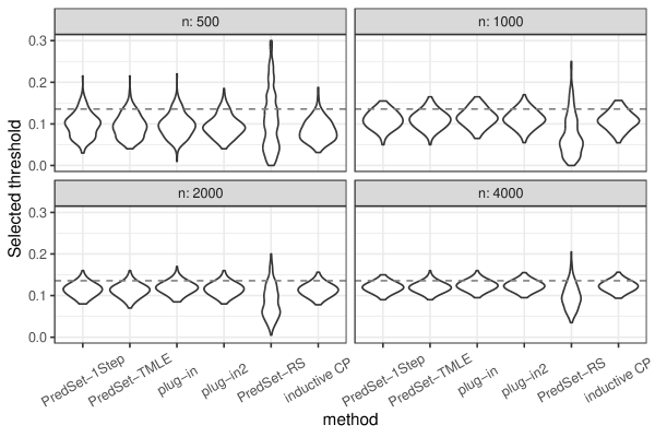
Figure S6: Violin plot of the sampling distribution of the selected threshold $\hat{\tau}_{n}$ in the low dimensional setting. The gray horizontal dashed line is the true optimal threshold $\tau_{0}$.

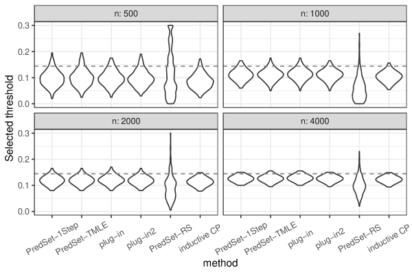
Figure S8: Violin plot of the sampling distribution of the selected threshold $\hat{\tau}_{n}$ in the low dimensional setting without covariate shift. The gray horizontal dashed line is the true optimal threshold $\tau_{0}$.

References

- Angelopoulos et al. (2021) Angelopoulos, A. N., S. Bates, E. J. Candès, M. I. Jordan, and L. Lei (2021). Learn then Test: Calibrating Predictive Algorithms to Achieve Risk Control. arXiv preprint arXiv:2110.01052v5.
- Bang and Robins (2005) Bang, H. and J. M. Robins (2005). Doubly robust estimation in missing data and causal inference models. Biometrics 61(4), 962–973.
- Bates et al. (2021) Bates, S., A. Angelopoulos, L. Lei, J. Malik, and M. I. Jordan (2021). Distribution-free, risk-controlling prediction sets. arXiv preprint arXiv:2101.02703.
- Berkenkamp et al. (2017) Berkenkamp, F., M. Turchetta, A. P. Schoellig, and A. Krause (2017). Safe model-based reinforcement learning with stability guarantees. Advances in Neural Information Processing Systems 2017-Decem, 909–919.
- Bickel et al. (1993) Bickel, P., C. A. Klaassen, Y. Ritov, and J. A. Wellner (1993). Efficient and adaptive estimation for semiparametric models. Johns Hopkins University Press.
- Bickel (1982) Bickel, P. J. (1982). On adaptive estimation. The Annals of Statistics, 647–671.
- Bickel and Ritov (2003) Bickel, P. J. and Y. Ritov (2003). Nonparametric estimators which can be “plugged-in”. Annals of Statistics 31(4), 1033–1053.
- Bickel et al. (2007) Bickel, S., M. Brückner, and T. Scheffer (2007). Discriminative learning for differing training and test distributions. ACM International Conference Proceeding Series 227, 81–88.
- Bindele et al. (2018) Bindele, H. F., A. Abebe, and N. K. Meyer (2018). Robust confidence regions for the semi-parametric regression model with responses missing at random. Statistics 52(4), 885–900.
- Bojarski et al. (2016) Bojarski, M., D. Del Testa, D. Dworakowski, B. Firner, B. Flepp, P. Goyal, L. D. Jackel, M. Monfort, U. Muller, J. Zhang, X. Zhang, J. Zhao, and K. Zieba (2016). End to End Learning for Self-Driving Cars. arXiv preprint arXiv:1604.07316v1.
- Cauchois et al. (2020) Cauchois, M., S. Gupta, A. Ali, and J. C. Duchi (2020). Robust Validation: Confident Predictions Even When Distributions Shift. arXiv preprint arXiv:2008.04267v1.
- Chen (2007) Chen, X. (2007). Chapter 76: Large Sample Sieve Estimation of Semi-Nonparametric Models. Handbook of Econometrics 6(SUPPL. PART B), 5549–5632.
- Chernozhukov et al. (2018) Chernozhukov, V., D. Chetverikov, M. Demirer, E. Duflo, C. Hansen, W. Newey, and J. Robins (2018). Double/debiased machine learning for treatment and structural parameters. Econometrics Journal 21(1), C1–C68.
- Chernozhukov et al. (2018) Chernozhukov, V., K. Wuthrich, and Y. Zhu (2018). Exact and Robust Conformal Inference Methods for Predictive Machine Learning With Dependent Data. In Proceedings of the 31st Conference On Learning Theory, PMLR, Volume 75, pp. 732–749. PMLR.
- Dunn et al. (2018) Dunn, R., L. Wasserman, and A. Ramdas (2018). Distribution-free prediction sets with random effects. arXiv preprint arXiv:1809.07441.
- Friedman (2004) Friedman, J. (2004). On multivariate goodness-of-fit and two-sample testing. Technical report, Citeseer.
- Friedman (2001) Friedman, J. H. (2001). Greedy function approximation: A gradient boosting machine. Technical Report 5.
- Friedman (2002) Friedman, J. H. (2002). Stochastic gradient boosting. Computational Statistics and Data Analysis 38(4), 367–378.
- Gal et al. (2017) Gal, Y., R. Islam, and Z. Ghahramani (2017). Deep Bayesian active learning with image data. In 34th International Conference on Machine Learning, ICML 2017, Volume 3, pp. 1923–1932. PMLR.
- Groenwold et al. (2012) Groenwold, R. H., I. R. White, A. R. T. Donders, J. R. Carpenter, D. G. Altman, and K. G. Moons (2012). Missing covariate data in clinical research: When and when not to use the missing-indicator method for analysis. Cmaj 184(11), 1265–1269.
- Hahn (1998) Hahn, J. (1998). On the Role of the Propensity Score in Efficient Semiparametric Estimation of Average Treatment Effects. Econometrica 66(2), 315.
- Hajek (1962) Hajek, J. (1962). Asymptotically Most Powerful Rank-Order Tests. The Annals of Mathematical Statistics 33(3), 1124–1147.
- Hall (2013) Hall, P. (2013). The bootstrap and Edgeworth expansion. Springer Science & Business Media.
- Han and Kato (2019) Han, Q. and K. Kato (2019). Berry-Esseen bounds for Chernoff-type non-standard asymptotics in isotonic regression. arXiv preprint arXiv:1910.09662v2.
- Hastie et al. (1995) Hastie, T., A. Buja, and R. Tibshirani (1995). Penalized discriminant analysis. Ann. Statist. 23(1), 73–102.
- Hastie and Tibshirani (1990) Hastie, T. J. and R. J. Tibshirani (1990). Generalized Additive Models. Chapman and Hall/CRC.
- Hendrycks and Dietterich (2019) Hendrycks, D. and T. Dietterich (2019). Benchmarking neural network robustness to common corruptions and perturbations. 7th International Conference on Learning Representations, ICLR 2019.
- Kennedy (2022) Kennedy, E. H. (2022). Semiparametric doubly robust targeted double machine learning: a review. arXiv preprint arXiv:2203.06469.
- Kitani et al. (2012) Kitani, K. M., B. D. Ziebart, J. A. Bagnell, and M. Hebert (2012). Activity forecasting. Lecture Notes in Computer Science (including subseries Lecture Notes in Artificial Intelligence and Lecture Notes in Bioinformatics) 7575 LNCS(PART 4), 201–214.
- Le Cam (1969) Le Cam, L. M. (1969). Théorie asymptotique de la décision statistique, Volume 33. Presses de l’Université de Montréal.
- Lei et al. (2018) Lei, J., M. G’Sell, A. Rinaldo, R. J. Tibshirani, and L. Wasserman (2018). Distribution-Free Predictive Inference for Regression. Journal of the American Statistical Association 113(523), 1094–1111.
- Lei et al. (2015) Lei, J., A. Rinaldo, and L. Wasserman (2015). A conformal prediction approach to explore functional data. Annals of Mathematics and Artificial Intelligence 74(1), 29–43.
- Lei et al. (2013) Lei, J., J. Robins, and L. Wasserman (2013). Distribution-free prediction sets. Journal of the American Statistical Association 108(501), 278–287.
- Lei and Wasserman (2014) Lei, J. and L. Wasserman (2014). Distribution-free prediction bands for non-parametric regression. Journal of the Royal Statistical Society. Series B: Statistical Methodology 76(1), 71–96.
- Lei and Candès (2021) Lei, L. and E. J. Candès (2021). Conformal inference of counterfactuals and individual treatment effects. Journal of the Royal Statistical Society. Series B: Statistical Methodology 83(5), 911–938.
- Levit (1974) Levit, B. Y. (1974). On optimality of some statistical estimates. In Proceedings of the Prague symposium on asymptotic statistics, Volume 2, pp. 215–238. Charles University Prague.
- Little and Rubin (2019) Little, R. J. and D. B. Rubin (2019). Statistical analysis with missing data. John Wiley & Sons, Ltd.
- Malik et al. (2019) Malik, A., V. Kuleshov, J. Song, D. Nemer, H. Seymour, and S. Ermon (2019). Calibrated Model-Based Deep Reinforcement Learning. In 36th International Conference on Machine Learning, ICML 2019, pp. 4314–4323. PMLR.
- Mason et al. (1999) Mason, L., J. Baxter, P. Bartlett, and M. Frean (1999). Boosting Algorithms as Gradient Descent in Function Space. Technical report.
- Mason et al. (2000) Mason, L., J. Baxter, P. L. Bartlett, and M. Frean (2000). Boosting Algorithms as Gradient Descent. Technical report.
- Matsouaka et al. (2023) Matsouaka, R. A., Y. Liu, and Y. Zhou (2023). Variance estimation for the average treatment effects on the treated and on the controls. Statistical Methods in Medical Research 32(2), 389–403.
- Menon and Ong (2016) Menon, A. K. and C. S. Ong (2016). Linking losses for density ratio and class-probability estimation. In 33rd International Conference on Machine Learning, ICML 2016, Volume 1, pp. 484–504. PMLR.
- Moja et al. (2014) Moja, L., K. H. Kwag, T. Lytras, L. Bertizzolo, L. Brandt, V. Pecoraro, G. Rigon, A. Vaona, F. Ruggiero, M. Mangia, A. Iorio, I. Kunnamo, and S. Bonovas (2014). Effectiveness of computerized decision support systems linked to electronic health records: A systematic review and meta-analysis. American Journal of Public Health 104(12), e12–e22.
- Newey et al. (1998) Newey, W., F. Hsieh, and J. Robins (1998). Undersmoothing and Bias Corrected Functional Estimation.
- Newey (1990) Newey, W. K. (1990). Semiparametric efficiency bounds. Journal of Applied Econometrics 5(2), 99–135.
- Newey et al. (2004) Newey, W. K., F. Hsieh, and J. M. Robins (2004). Twicing Kernels and a Small Bias Property of Semiparametric Estimators. Econometrica 72(3), 947–962.
- Papadopoulos et al. (2002) Papadopoulos, H., K. Proedrou, V. Vovk, and A. Gammerman (2002). Inductive confidence machines for regression. In European Conference on Machine Learning, pp. 345–356. Springer.
- Park et al. (2021) Park, S., E. Dobriban, I. Lee, and O. Bastani (2021). Pac prediction sets under covariate shift.
- Park et al. (2020) Park, S., S. Li, I. Lee, and O. Bastani (2020). Pac confidence predictions for deep neural network classifiers. arXiv preprint arXiv:2011.00716.
- Pfanzagl (1985) Pfanzagl, J. (1985). Contributions to a general asymptotic statistical theory, Volume 3 of Lecture Notes in Statistics. New York, NY: Springer New York.
- Pfanzagl (1990) Pfanzagl, J. (1990). Estimation in semiparametric models, Volume 63 of Lecture Notes in Statistics. Springer, New York, NY.
- Qiu et al. (2021) Qiu, H., A. Luedtke, and M. Carone (2021). Universal sieve-based strategies for efficient estimation using machine learning tools. Bernoulli 27(4), 2300–2336.
- Quiñonero-Candela et al. (2009) Quiñonero-Candela, J., M. Sugiyama, N. D. Lawrence, and A. Schwaighofer (2009). Dataset shift in machine learning. Mit Press.
- Ren et al. (2017) Ren, S., K. He, R. Girshick, and J. Sun (2017). Faster R-CNN: Towards Real-Time Object Detection with Region Proposal Networks. IEEE Transactions on Pattern Analysis and Machine Intelligence 39(6), 1137–1149.
- Robins (2000) Robins, J. M. (2000). Robust estimation in sequentially ignorable missing data and causal inference models. In Proceedings of the American Statistical Association, Volume 1999, pp. 6–10.
- Rosenbaum and Rubin (1983) Rosenbaum, P. R. and D. B. Rubin (1983). The central role of the propensity score in observational studies for causal effects. Biometrika 70(1), 41–55.
- Rothe (2017) Rothe, C. (2017). Robust Confidence Intervals for Average Treatment Effects Under Limited Overlap. Econometrica 85(2), 645–660.
- Rotnitzky et al. (2021) Rotnitzky, A., E. Smucler, and J. M. Robins (2021). Characterization of parameters with a mixed bias property. Biometrika 108(1), 231–238.
- Sadinle et al. (2019) Sadinle, M., J. Lei, and L. Wasserman (2019). Least Ambiguous Set-Valued Classifiers With Bounded Error Levels. Journal of the American Statistical Association 114(525), 223–234.
- Saunders et al. (1999) Saunders, C., A. Gammerman, and V. Vovk (1999). Transduction with confidence and credibility. In IJCAI.
- Scharfstein et al. (1999) Scharfstein, D. O., A. Rotnitzky, and J. M. Robins (1999). Adjusting for Nonignorable Drop-Out Using Semiparametric Nonresponse Models. Journal of the American Statistical Association 94(448), 1096–1120.
- Scheffe and Tukey (1945) Scheffe, H. and J. W. Tukey (1945). Non-parametric estimation. i. validation of order statistics. The Annals of Mathematical Statistics 16(2), 187–192.
- Schick (1986) Schick, A. (1986). On asymptotically efficient estimation in semiparametric models. The Annals of Statistics, 1139–1151.
- Shah and Peters (2020) Shah, R. D. and J. Peters (2020). The hardness of conditional independence testing and the generalised covariance measure. Annals of Statistics 48(3), 1514–1538.
- Shen (1997) Shen, X. (1997). On methods of sieves and penalization. Annals of Statistics 25(6), 2555–2591.
- Shimodaira (2000) Shimodaira, H. (2000). Improving predictive inference under covariate shift by weighting the log-likelihood function. Journal of statistical planning and inference 90(2), 227–244.
- Sugiyama and Kawanabe (2012) Sugiyama, M. and M. Kawanabe (2012). Machine learning in non-stationary environments : introduction to covariate shift adaptation. MIT Press.
- Sugiyama et al. (2008) Sugiyama, M., T. Suzuki, S. Nakajima, H. Kashima, P. Von Bünau, and M. Kawanabe (2008). Direct importance estimation for covariate shift adaptation. Annals of the Institute of Statistical Mathematics 60(4), 699–746.
- Szegedy et al. (2014) Szegedy, C., W. Zaremba, I. Sutskever, J. Bruna, D. Erhan, I. Goodfellow, and R. Fergus (2014). Intriguing properties of neural networks. 2nd International Conference on Learning Representations, ICLR 2014 - Conference Track Proceedings.
- Tanser et al. (2013) Tanser, F., T. Bärnighausen, E. Grapsa, J. Zaidi, and M. L. Newell (2013). High coverage of ART associated with decline in risk of HIV acquisition in rural KwaZulu-Natal, South Africa. Science 339(6122), 966–971.
- Tibshirani (1996) Tibshirani, R. (1996). Regression shrinkage and selection via the lasso. J. R. Stat. Soc. Ser. B. Stat. Methodol. 58(1), 267–288.
- Tibshirani et al. (2019) Tibshirani, R. J., R. F. Barber, E. J. Candès, and A. Ramdas (2019). Conformal prediction under covariate shift. Advances in Neural Information Processing Systems 32.
- Tran et al. (2018) Tran, L., M. Petersen, J. Schwab, and M. J. van der Laan (2018). Robust variance estimation and inference for causal effect estimation. arXiv preprint arXiv:1810.03030.
- Tukey (1947) Tukey, J. W. (1947). Non-parametric estimation ii. statistically equivalent blocks and tolerance regions–the continuous case. The Annals of Mathematical Statistics, 529–539.
- Tukey (1948) Tukey, J. W. (1948). Nonparametric estimation, iii. statistically equivalent blocks and multivariate tolerance regions–the discontinuous case. The Annals of Mathematical Statistics, 30–39.
- van der Laan et al. (2007) van der Laan, M. J., E. C. Polley, and A. E. Hubbard (2007). Super Learner. Statistical Applications in Genetics and Molecular Biology 6(1).
- Van der Laan and Rose (2018) Van der Laan, M. J. and S. Rose (2018). Targeted learning in data science: causal inference for complex longitudinal studies. Springer.
- Van der Laan and Rubin (2006) Van der Laan, M. J. and D. Rubin (2006). Targeted maximum likelihood learning. The international journal of biostatistics 2(1).
- Van Der Vaart (1991) Van Der Vaart, A. (1991). On Differentiable Functionals. The Annals of Statistics 19(1), 178—-204.
- van der Vaart (1998) van der Vaart, A. W. (1998). Asymptotic Statistics. Cambridge University Press.
- van der Vaart and Wellner (1996) van der Vaart, A. W. and J. Wellner (1996). Weak convergence and empirical processes: with applications to statistics. Springer Science & Business Media.
- Vovk (2013) Vovk, V. (2013). Conditional validity of inductive conformal predictors. In Asian conference on machine learning, Volume 25, pp. 475–490. PMLR.
- Vovk et al. (1999) Vovk, V., A. Gammerman, and C. Saunders (1999). Machine-learning applications of algorithmic randomness. In International Conference on Machine Learning.
- Vovk et al. (2005) Vovk, V., A. Gammerman, and G. Shafer (2005). Algorithmic learning in a random world. Springer Science & Business Media.
- Wald (1943) Wald, A. (1943). An Extension of Wilks’ Method for Setting Tolerance Limits. The Annals of Mathematical Statistics 14(1), 45–55.
- Wilks (1941) Wilks, S. S. (1941). Determination of Sample Sizes for Setting Tolerance Limits. The Annals of Mathematical Statistics 12(1), 91–96.
- Yang et al. (2022) Yang, Y., A. K. Kuchibhotla, and E. T. Tchetgen (2022). Doubly Robust Calibration of Prediction Sets under Covariate Shift. arXiv preprint arXiv:2203.01761.
- Zhang and Liang (2011) Zhang, J. J. and H. Y. Liang (2011). Berry-Esseen type bounds in heteroscedastic semi-parametric model. Journal of Statistical Planning and Inference 141(11), 3447–3462.