Stochastic Learning in Kolkata Paise Restaurant Problem: Classical & Quantum Strategies

Abstract

We will review the results for stochastic learning strategies, both classical (one-shot and iterative) and quantum (one-shot only), for optimizing the available many-choice resources among a large number of competing agents, developed over the last decade in the context of the Kolkata Paise Restaurant Problem. Apart from a few rigorous and approximate analytical results, both for classical and quantum strategies, most of the interesting results on the phase transition behavior (obtained so far for the classical model) using classical Monte Carlo simulations. All these, including the applications to computer science (job or resource allotments in Internet-of-Things), transport engineering (on-line vehicle hire problems), operation research (optimizing efforts for delegated search problem, efficient solution of Travelling Salesman problem), etc will be discussed.

1 Introduction

Game theory was initially evolved to investigate different strategic situations with competing players [1]. Of late, the concept of game theory is being applied to different statistical events to measure the success rate when one’s success depends on the choice of the other agents. The game of Prisoners’ dilemma (see e.g., [2]) is a popular example where two non-communicating (or non-interacting) agents choose their actions from two possible choices. It is a two-person, two-choice, one-shot (one time decision) game. The Nash equilibrium (see e.g., [3]) solution employs the strategy, where the other player can not gain from any of the choices, and both the players necessarily defect. However, this is not a Pareto optimal solution (see e.g., [4]), where no change in the decision can lead to a gain for one player without any loss of the other. This problem has been used to model many real life problems like auction bidding, arms races, oligopoly pricing, political bargaining, salesman effort etc.

The minority game theory (see e.g., [5]) generalizes this idea of a very large number of non-communicating players with with two choices for each of them. As the name suggests, the players who make the minority group choice (at any time) receive a payoff. This game is not an one-shot game and the players learn from their previous mistakes (loss of payoffs) and continuously try upgrade their respective respective strategies to gain the payoffs and they (the society as a whole) learn collectively to reach a level of maximum efficiency, where no one can improve their payoff any further. A phase transition (see e.g., [5]) occurs at a critical value the memory size (number of distinct strategies individually remembered; assumed to be the same for all the players [6]) and the number of players and the socially optimal learning tome diverges at this critical point. The game has many important application of social dilemmas, including a decision of making investment in a stock market; over-crowding of the agents any day due to decision either buying or selling a particular stock in a financial market can lead to loss for the majority players!

The minority game is further generalized for many choices in addition to many players (as the minority game) in the Kolkata Paise Restaurant (KPR) game theory, introduced by Chakrabarti [7] and Chakrabarti et al. [8] (for a recent review see e.g., Chakrabarti et al. [9]). The KPR game is also an iterative game, played by the agents or players without any interaction or communication between each other.

In Kolkata, long back, there were very cheap and fixed price “Paise Restaurants” (also called “Paise Hotels”; Paise was the smallest Indian coin) which were very popular among the daily laborers in the city. During lunch hours, these laborers used to walk down (to save the transport costs) from their place of work to one of these restaurants. These Paise Restaurants would prepare every day a fixed (small) number of such dishes, and if several groups of laborers would arrive any day to the same restaurant, only one group perhaps would get their lunch and the rest would miss lunch that day. There were no cheap communication means (mobile phones) for mutual interactions, in order to decide about the respective restaurants of the day. Walking down to the next restaurant would mean failing to report back to work on time! To complicate this collective learning and decision making problem, there were indeed some well-known rankings of these restaurants, as some of them would offer tastier items compared to the others (at thesame cost, paisa, of course) and people would prefer to choose the higher rank of the restaurant, if not crowded! This “mismatch” of the choice and the consequent decision not only creates inconvenience for the prospective customer (going without lunch), would also mean “social wastage” (excess unconsumed food, services or supplies somewhere).

A similar problem arises when the public administration plans and provides hospitals (beds) in different localities, but the local patients prefer “better” perceived hospitals elsewhere. These “outsider” patients then compete with the local patients and have to choose other suitable hospitals elsewhere. Unavailability of the hospital beds in the over-crowded hospitals may be considered as insufficient service provided by the administration, and consequently the unattended potential services will be considered as social wastage. This kind of games, anticipating the possible strategies of the other players and acting accordingly, is very common in society. Here, the number of choices need not be very limited (as in the standard binary-choice formulations of most of the games) and the number of players can be truly large! Also, these are not necessarily one shot games, rather the players can learn from past mistakes and improve on the selection of their strategies for the next move. These features make the games extremely intriguing and also versatile, with major collective or social emerging structures.

The KPR problem seems to have a trivial solution: suppose that somebody, say a dictator (who is not a player), assigns a restaurant to each person and asks them to shift to the next restaurant cyclically, on successive evenings. The fairest and most efficient solution: each customer gets food on each evening (if the number of plates or choices is the same as that of the customers or players) with the same share of the rankings as others, and that too from the first evening (minimum evolution time). This, however, is not a true solution of the KPR problem, where each customer or agent decides on his or her own every evening, based on complete information about past events. Several recent applications of the classical KPR strategies to Vehicle for Online Hire problem [10, 11], resource allocation problem in the context of Internet-of-Things [12], developing a different strategy for solving the the Traveling Salesman Problem [13], etc have been made.

For the last few decades, quantum game theory has been developed, promising more success over classical strategies  [14, 15, 16, 17, 18, 19, 20, 21]. This is an interdisciplinary approach that connects three different fields: quantum mechanics, information theory and game theory in a concrete way. Quantum game theory offers different protocols that are based on the uses of quantum mechanical phenomena like entanglement, quantum superposition, and interference arising due to wave mechanical aspects of such systems. In context of game theory, quantum strategies are first introduced in two papers by Meyer [14] and by Eisert et al. [15] where they showed that a player performing a quantum move wins against a player performing a classical move regardless of their classical choices. The advantage of a quantum strategy over classical one has been specifically investigated in [15] for the case of Prisoners’ dilemma. This idea is generalized for multiple players by Benjamin and Hayden [16] with a specific solution for four players. The authors here introduced quantum minority game where they showed that an entanglement shared between the players promises better performance of quantum strategy over the classical one. Chen et al. [22] further extends this result of quantum minority game for $N$-players.

Since then, different aspects of multi-player minority games are being studied extensively. As already mentioned, the KPR problem is a minority game with a large number of choices for each of the players, who are also equally large in number. In 2011, Sharif and Heydari [23] introduced the quantum version of the KPR game, with a solution for three agents and three choices. This study was later extended by Sharif and Haydari [24] in 2012, Ramzan [25] and Sharif and Haydari [26] in 2013 for the three and multi-player quantum minority games, including the quantum KPR games (essentially one-shot solutions). For a detailed discussion see Chakrabarti et al. [9].

We review here the statistics of the KPR problem employing both classical and quantum strategies. The article is organized as follows. In Sec. 2, we describe the classical strategies of KPR game and show that there exists a phase transition when the number of customers is less than the number of restaurants. We also discuss there the possible ways by which we can minimize the social wastage fraction. In Sec. 3, we first discuss about the general setting of quantum games and then provides a flavour of two game theoretical problems, such as, Prisoners’ dilemma and minority game in the context of both classical and quantum strategies. In Sec. 4, we introduce quantum version of KPR problem. We review here the results of one shoot quantum KPR problem with three players and three choices by Sharif and Haydari [23, 24, 27], and Ramzan [25]. We show that using quantum strategies one can gain in payoff by $50\%$ compared to the classical strategies for one shoot KPR game with three players and three choices. We also discuss about the effect of entanglement and decoherence (or loss of phase coherence) in finding the expected payoff of a player for the mentioned game problem.

2 Statistics of KPR game: Classical strategies

Let us consider the KPR game with $N$ restaurants and $\lambda N$ non-communicating players (agents or customers). We assume that every day or evening or time ($t$), each restaurant prepares only one dish (generalization to a larger number would not affect the statistics of the game). As discussed, every time $t$, the objective of each of the player is to choose one among $N$ restaurant such that she will be alone there in order to get the only dish. If some restaurant is visited by more than one customer, then the restaurant selects one of them randomly and serve the dish to her; thus rest of the visitors there would remain unhappy by starving that evening.

Let us consider first the random choice (no learning) case where each player chooses randomly any of the restaurants. Then the probability $P$ of choosing one restaurant by $n~{}(\leq N)$ players is

$$P(n)=\binom{\lambda N}{n}{p}^{n}{(1-p)}^{\lambda N-n};~{}p=\frac{1}{N}.$$ (1)

In the case $N$ goes to infinity, we get

$$P(n)=\frac{\lambda^{n}}{n!}exp(-\lambda).$$ (2)

Hence, the fraction $P(n=0)$ of restaurants not chosen by any customer is $exp(-\lambda)$. The fraction of restaurants chosen by at least one customer on any evening is therefore gives the utilization fraction [8]

$$f=1-exp(-\lambda).$$ (3)

If $N$ agents (where $\lambda=1$) randomly choose and visit any one among $N$ restaurants then utilization fraction $f$ becomes $1-exp(-1)\simeq 0.63$. Since there is no iterative learning for this case, every time the utilization fraction will be about $63\%$ starting from the first day (convergence time $\tau$ = 0).

It may be noted that a dictated solution to the KPR problem is simple and very efficient from the first day. The Dictator is not a player in the game and asks the players to form a queue (with periodic boundary condition), visit a restaurant according to her respective positions in that queue and continue shifting by one step every day. Every player gets a dish and hence the steady state ($t$-independent) social utilization fraction $f$ becomes maximum (unity) from the first day ($\tau=1$). This dictated solution is applicable even when the restaurants have ranks (agreed by all the customers) i.e. agents have their preferences over the restaurants. Thus the dictated solution is very efficient in achieving maximum utility from the first day $(f=1,\tau=1)$. However no choice of the individual is considered here and in a democratic set-up no such a dictatorial strategy is acceptable.

We now consider the case where the players try to learn and update their strategies of choosing a restaurant to avoid overcrowding the chosen restaurant. As already discussed, we measure the social utilization fraction $f(t)$ on any day $t$ as

$$f(t)=\sum_{i=1}^{N}[\delta(n_{i}(t))/\lambda N],$$ (4)

where $\delta(n)=1$ for $n\geq 1$ and $\delta(n)=0$ for $n=0$; $n_{i}(t)$ denotes the number of customers arriving at the $i$th (rank if customer choice is considered) restaurant on $t$ th evening. The goal is to learn collectively towards achieving $f(t)$ = 1 preferably in finite convergence time $\tau$, i.e., $f(t)$ = 1 for $t\geq\tau$, where $\tau$ is finite.

Earlier studies (see e.g., [8, 9, 28, 29, 30, 31]) had proposed several learning strategies for KPR game. In references [29, 30, 31, 32], the authors had studied several stochastic crowd avoidance learning strategies leading to increased utilization fraction (compared to the random choice case Eq. (3)). In some of the cases this is achieved ($f=1$) at a critical point [6] where $\tau$ goes to infinity due to critical slowing down.

Here we discuss numerical (Monte Carlo) results for the statistics of KPR game where $\lambda N$ ($\lambda>0$) customers choose one among $N$ restaurants following a strategy discussed next. On day $t$, an agent goes back to her last day’s visited restaurant $k$ with probability

$$p_{k}(t)={[n_{k}(t-1)]}^{-\alpha};~{}\alpha>0$$ (5a)

and chooses a different restaurant $$(k^{{}^{\prime}}\neq k) N-1$$ among any of the () neighboring restaurants, with probability

$$p_{k^{{}^{\prime}}}(t)=(1-p_{k}(t))/(N-1).$$ (5b)

These “learning” strategies employed by the players, for the choice of restaurants placed on different dimensional ($d$) lattices. In infinite dimension (mean field case) the restaurant indices $k$ and $k^{{}^{\prime}}$ in Eq. (5a, 5b) run from $1$ to $N$ of the lattice. For finite dimensions $k$ runs from $1$ to $N$ while $k^{{}^{\prime}}$ corresponds to the nearest neighbour of the $k$ th restaurant on the lattice.

Authors in [30] had studied crowd dynamics with $\alpha=1,\lambda=1$ in infinite, $2d$, $1d$ lattice structure of restaurants. KPR dynamics for $\alpha\leq 1,\lambda=1$ had been studied in [31] for infinite, $3d,2d,1d$ lattice structure of restaurants. Phase transition behaviours are observed for $\alpha$ near $\alpha_{c}=0_{+}$ for infinite, $3d$ and $2d$ lattice structure of the restaurants. The steady state statistics are studied when the utilization fraction $f(t)$ remains the same (within a predefined margin) for further iterations. The steady state wastage fraction $(1-f)$ and the convergence time $\tau$ for reaching the steady state are found to vary with $\Delta\alpha\equiv|\alpha-\alpha_{c}|$ as $(1-f)\sim\Delta\alpha^{\beta}$ and $\tau\sim\Delta\alpha^{-\gamma}$ with $\beta\simeq 0.8,0.87,1.0$ and $\gamma\simeq 1.18,1.11,1.05$ in infinite-dimension, $3d$ and $2d$ lattice structures respectively. Results of $1d$ lattice structure is found to be trivial unlike other dimensions and no phase transition ($f$ reaches unity with no divergence in $\tau$) is seen for any $\alpha>0$.

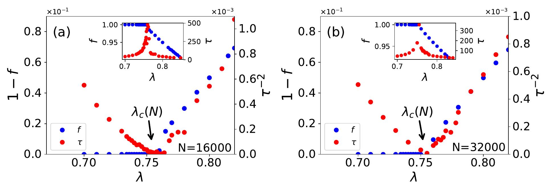
Figure 1: Plots of steady state convergence behaviour in infinite dimensional lattice; Social wastage fraction $(1-f)$ and convergence time $\tau$ against customer fraction $\lambda$. Observed power laws are $(1-f)\sim\Delta\lambda^{\beta}$ where $\beta=1.0\pm 0.02$ and $\tau\sim\Delta\lambda^{-\gamma}$ where $\gamma=0.5\pm 0.02$. Here $\Delta\lambda\equiv|\lambda-\lambda_{c}(N)|$. The insets show the variation of $f$ and $\tau$ against $\lambda$, showing the diverging behaviour of $\tau$ where $f$ reaches unity at $\lambda=\lambda_{c}(N)$. (a) for $N=16000$ and (b) for $N=32000$.

Here we discuss the numerical results for the Monte Carlo studies on steady state statistics of the KPR game dynamics for general $\alpha$ and $\lambda$ cases. In the case where $\alpha=1$ and $\lambda$ is $<1$, we find power law fits for social wastage fraction $(1-f)\sim\Delta\lambda^{\beta}$ and convergence time $\tau\sim\Delta\lambda^{-\gamma}$ with $\beta=1.0\pm 0.02$ and $\gamma=0.5\pm 0.02$ in infinite dimension with $\Delta\lambda\equiv|\lambda-\lambda_{c}|$, where $\lambda_{c}=0.74\pm 0.01$ (see Figs 1, 2). For finite size $N$, we observe the effective critical point $\lambda_{c}(N)$ for which the finite size scaling (see Fig. 2) gives best fit for $d\nu=2.0$ and $\lambda_{c}=0.74\pm 0.01$.

A crude estimate of the mean field value of $\lambda_{c}$ can be obtained as follows. Here $\lambda N$ agents choose every day among the $N$ restaurants. Hence the probability of any restaurant to be chosen by a player is $\frac{\lambda N}{N}=\lambda$ and the fraction of restaurants not visited by any player will be $(1-\lambda)$. In the steady state, the number of players $n$ choosing any restaurant can be 0, 1, 2, 3,… . If we assume the maximum crowd size at any restaurant on any day to be 2, then the probability of those restaurants to go vacant next day will be $(\frac{1}{2})^{2}$. Hence the critical value $\lambda_{c}$ of $\lambda$ in the steady state will be given by

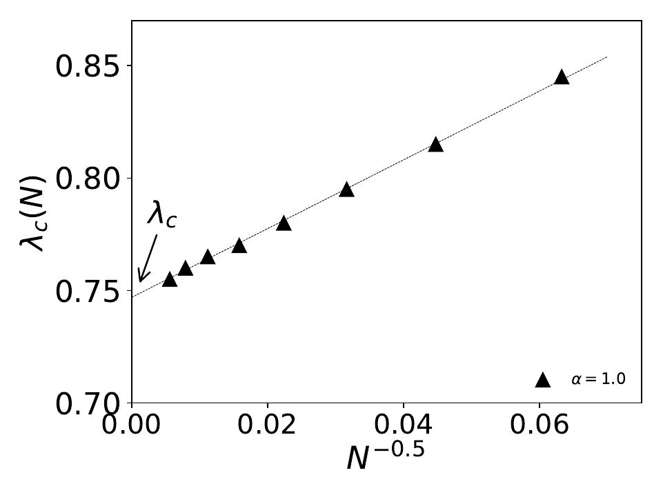
Figure 2: Extrapolation study of the effective finite size dependent critical density of customers $\lambda_{c}(N)$. The system size dependence is fitted to $\frac{1}{\sqrt{N}}$ and we get $\lambda_{c}=0.74\pm 0.01$ for $\lambda_{c}\equiv\lambda_{c}(N\to\infty)$.

$$1-\lambda_{c}=\frac{1}{4},$$ (6)

giving $\lambda_{c}\simeq 0.75$ . For more details see [30].

3 Quantum Games

In the setting of quantum games, the $N$ different choices of any arbitrary player or agent are encoded in the basis states of a $N$-level quantum system that acts as a subsystem with $N$-dimensional Hilbert space. The total system for $M$ ($=\lambda N$ as defined in Sec. 2) players or agents can be represented by a state vector in a $\prod_{i=1}^{M}{\rm dim}(\mathcal{H}_{\mathcal{L}_{i}})$ dimensional Hilbert space $\mathcal{H}_{\mathcal{L}}=\mathcal{H}_{\mathcal{L}_{M}}\otimes\mathcal{H}_{\mathcal{L}_{n-1}}\cdots\otimes\mathcal{H}_{\mathcal{L}_{1}}$, where $\mathcal{H}_{\mathcal{L}_{i}}$ is the Hilbert space of the $i$-th subsystem. The different subsystems are distributed among the players and the initial state of the total system is chosen so that the subsystems become entangled. The players do not communicate among each other before choosing a strategy. A strategy move in quantum games is executed by the application of local operators associated to each player on the quantum state. The players do not have access any other parts of the system except their own subsystems. In addition, no information is shared between the players exploiting the quantum nature of the game. The quantum strategies are indeed the generalized form of classical strategies with $s_{i}\in S_{i}\;\Rightarrow\;U_{i}\in\textrm{S}(N_{i})$, where the set of permitted local quantum operations $\textrm{S}(N_{i})$ is some subset of the special unitary group $\textrm{SU}(N_{i})$.

We will now describe different steps of the quantum game protocol [27]. The game starts with an initial entangled state $|\psi_{n}\rangle$ shared by different players. We have considered the subsystems of the same dimension $N$ that indeed denotes the number of pure strategies available to each player. The number of subsystems is equal to the number of players. It can be thought that $|\psi_{n}\rangle$ has been prepared by a referee who distributes the subsystems among the players. By choosing a unitary operator $U$ from a subset of SU($N$), the players apply that on their subsystems and, the final state is given by

$$\rho_{\rm fin}=U\otimes U\otimes\cdots\otimes U\rho_{\rm in}U^{\dagger}\otimes U^{\dagger}\otimes\cdots\otimes U^{\dagger},$$ (7)

where $\rho_{\rm in}$ and $\rho_{\rm fin}$ are the initial and final density matrix of the system, respectively. Due to the symmetry of the games and, since the players do not communicate among themselves, they are supposed to do the same operation. The advantage of quantum game over classical one is that it reduces the probability of collapsing the final state $\rho_{\rm fin}$ to the basis states that have lower or zero payoff $\$$. Since quantum mechanics is a fundamentally probabilistic theory, the only notion of payoff after a strategic move is the expected payoff. To evaluate the expected payoffs, the first step is to define a payoff operator $P_{i}$ for an arbitrary player $i$ and that can be written as

$$P_{i}=\sum_{j}\$^{j}_{i}|\alpha^{j}_{i}\rangle\langle\alpha^{j}_{i}|,$$ (8)

where $\$_{i}^{j}$ are the associated payoffs to the states $|\alpha^{j}_{i}\rangle$ for $i$-th player. The expected payoff $E_{i}(\$)$ of player $i$ is then calculated by considering the trace of the product of the final state $\rho_{\rm fin}$ and the payoff-operator $P_{i}$,

$$E_{i}(\$)=\mathrm{Tr\left(\mathit{P}_{i}\rho_{\rm fin}\right)}.$$ (9)

The Prisoners’ dilemma is a game with two players and both of them have two independent choices. In this game, two players, Alice and Bob choose to cooperate or defect without sharing any prior information about their actions. Depending on their combination of strategies, each player receives a particular payoff. Once Bob decides to cooperate, Alice receives payoff $\$_{A}=3$ if she also decides to cooperate, and she receives $\$_{A}=5$ if she decides to defect. On the other hand, if Bob sets his mind to defect, Alice receives $\$_{A}=1$ by following Bob and, $\$_{A}=0$ by making the other choice. It reflects that whatever Bob decides to choose, Alice will always gain if she decides to defect. Since there is no possibility of communications between the players, the same is true for Bob. This leads to a dominant strategy when both the players defect and they both have payoff $\$_{\rm A/B}=1$. In terms of game theory, this strategy of mutual defection is a Nash equilibrium, because none of the players can do better by changing their choices independently. However, it can be noted that this is not an efficient solution. Because there exists a Pareto optimal strategy when both the players cooperate, and they both receive $\$_{\rm A/B}=1$. This gives rise to a dilemma in this game. After a few decades, the quantum version of this game is introduced by J. Eisert, M. Wilkens, and M. Lewenstein in $1999$ [15]. In the quantum formulation, the possible outcomes of classical strategies (cooperate and defect) are represented by two basis vectors of a two-state system, i.e., a qubit. For this game, the initial state is considered as a maximally entangled Bell-type state, and the strategic moves for both the players are performed by the unitary operators from the subset of SU(2) group. In this scenario, a new Nash equilibrium is emerged in addition to the classical one, i.e., when both the players choose to defect. For the new case, the expected payoffs for both the players are found to be $E(\$_{A})=E(\$_{B})=3$. This is exactly the Pareto optimal solution for the classical pure strategy case. In the quantum domain, this also becomes a Nash equilibrium. Thus considering a particular quantum strategy one can always get a advantage over a classical strategy.

The above game is generalized for multiple players with two choices in the minority game theory. In this game, $n$ non-communicating agents independently make their actions from two available choices, and the main target of the players is to avoid the crowd. The choices are then compared and the players who belong to the smaller group are rewarded with payoff $\$=1$. If two choices are evenly distributed, or all the players make the same choice, no player will get any reward. To get the Nash equilibrium solution, the palyers must choose their moves randomly, since the deterministic strategy will lead to an undesired outcome where all the players go for the same choice. In this game, the expected payoff $E(\$)$ for a player can be calculated by the ratio of the number of outcomes that the player is in the minority group and the number of different possible outcomes. For a four-player game, the expected payoff of a player is found to be $1/8$, since each player has two minority outcomes out of sixteen possible outcomes. A quantum version of this game for four players was first introduces by Benjamin and Hayden in $2000$ [16]. They have shown that the quantum strategy provides a better performance than the classical one for this game. The application of quantum strategy reduces the probability of even distribution of the players between two choices, and this fact is indeed responsible for the outerperformance of quantum strategy over classical one. The quantum strategy provides an expected payoff $E(\$)=1/4$ for four-player game which is twice of the classical payoff.

4 Quantum KPR problem

As already mentioned, the Kolkata restaurant problem is a generalization of the minority game, where $\lambda N$ non-communicating agents or players generally have $N$ choices. The classical version of the KPR problem has been discussed in Sec. 2. This problem is also studied in quantum mechanical scenario, where the players are represented by different subsystems, and the basis states of the subsystems are different choices. To remind, for the KPR game, each of $\lambda N$ customers chooses a restaurant for getting the lunch from $N$ different choices in parallel decision mode. The players (customers) receive a payoff if their choice is not too crowded, i.e., the number of customers with the same choices is under some threshold limit. For this problem, this limit is considered as one. If more than one customer arrives at any restaurant for their lunch, then one of them is randomly chosen to provide the service, and the others will not get lunch on that day.

Let us consider a simple case of three players, say, Alice, Bob and Charlie who have three possible choices: restaurant $1$, restaurant $2$ and restaurant $3$. They receive a payoff $\$=1$ if they make a unique choice, otherwise they receive a payoff $\$=0$. Therefore, it is a one shoot game, i.e., non-iterative, and the players do not have any knowledge from previous rounds to decide their actions. Since the players can not communicate, there is no other way except randomizing between the choices. In this case, there are a total $27$ different combinations of choices and $12$ of that provide a payoff $\$=1$ to each of the players. Therefore, randomization between the choices leads to an expected payoff $E_{c}(\$)=4/9$ for each of the players using the classical strategy.

The quantum version of the KPR problem with three players ($M=3$; $\lambda=1$) and three choices ($N=3$) is first introduced by Sharif and Heydari [23]. In this case, Alice, Bob and Charlie share a quantum resource. Each of these players has a part in a multipartite quantum state. Whereas the classical players are allowed to randomize between their discrete set of choices, for the quantum version, each subsystem is allowed to be transformed by local quantum operations. Therefore, choosing a strategy or choice is equivalent to choose an unitary operator $U$. In absence of the entanglement in the initial state, it has been found that quantum games yield the same payoffs as its classical counterpart. On the other hand, it has been shown that sometimes a combination of unitary operators and entanglement outperform the classical randomization strategy.

In this particular KPR problem, the players have three choices, therefore, we need to deal with qutrits instead of qubits that are used for two choices to apply quantum protocols [27]. The local quantum operations on qutrits are performed by a complicated group of matrices from ${\rm SU}(3)$ group, unlike to the case of qubits where the local operators belong to ${\rm SU}(2)$ group. A qutrit is a three-level quantum system on three-dimensional Hilbert space $\mathcal{H_{\mathcal{L}}}=\textbf{C}^{3}$. The most general form of quantum state of a qutrit in the computational basis is given by

$$|\psi\rangle=c_{0}|0\rangle+c_{1}|1\rangle+c_{2}|2\rangle,$$ (10)

where $c_{0}$, $c_{1}$ and $c_{2}$ are three complex numbers satisfying the relation $|c_{0}|^{2}+|c_{1}|^{2}+|c_{2}|^{2}=1$. The basis states follow the orthonormal condition $\langle i|j\rangle=\delta_{i,j}$, where $i,j=0,1,2$. Then, the general state of a $n$-qutrit system can be written as a linear combination of $3^{n}$ orthonormal basis vectors:

$$\left|\Psi\right\rangle=\sum_{y_{n},..,y_{1}=0}^{2}c_{y_{n}...y_{1}}\left|y_{n}\cdots y_{1}\right\rangle,$$ (11)

where the basis vectors are the tensor product of individual qutrit states, defined as,

$$\left|y_{n}\cdots y_{1}\right\rangle=\left|y_{n}\right\rangle\otimes\left|y_{n-1}\right\rangle\otimes\cdots\otimes\left|y_{1}\right\rangle\in\mathcal{H_{\mathcal{L}}}=\overbrace{\textbf{C}^{3}\otimes...\otimes\textbf{C}^{3}}^{\textrm{$n$-times}},$$ (12)

with $y_{i}\in\{0,1,2\}$. The complex coefficients satisfy the normalization condition $\sum|c_{y_{n}...y_{1}}|^{2}=1$.

A single qutrit can be transformed by an unitary operator $U$ that belongs to special unitary group of degree $3$, denoted by SU($3$). In a system of $n$ qutrits, when an operation is performed only on a single qutrit, it is said to be local. The corresponding operation changes the state of that particular qutrit only. Under local operations, the state vector of a muti-qutrit system is transformed by the tensor products of individual operators, and the final state is given by

$$\left|\Psi_{\rm fin}\right\rangle=U_{n}\otimes U_{n-1}\otimes\cdots\otimes U_{1}\left|\Psi_{\rm in}\right\rangle,$$ (13)

where $|\Psi_{\rm in}\rangle$ is the initial state of the system.

The SU($3$) matrices, i.e., $3\times 3$ unitary matrices are parameterized by defining three orthogonal complex unit vectors $\bar{u},\bar{v},\bar{w}$, such that $\bar{u}\cdot\bar{v}=0$ and $\bar{u}^{*}\times\bar{v}=\bar{w}$ [33]. A general complex vector with unit norm is given by

$$\bar{u}=\left(\begin{array}[]{c}\sin\theta\cos\phi e^{i\alpha_{1}}\\ \sin\theta\sin\phi e^{i\alpha_{2}}\\ \cos\theta e^{i\alpha_{3}}\end{array}\right),$$ (14)

where $0\leq\phi,\theta\leq\pi/2$ and $0\leq\alpha_{1},\alpha_{2},\alpha_{3}\leq 2\pi$. An another complex unit vector satisfying $\bar{u}\cdot\bar{v}=0$ is given by

$$\bar{v}=\left(\begin{array}[]{c}\cos\chi\cos\theta\cos\phi e^{i(\beta_{1}-\alpha_{1})}+\sin\chi\sin\phi e^{i(\beta_{2}-\alpha_{1})}\\ \cos\chi\cos\theta\sin\phi e^{i(\beta_{1}-\alpha_{2})}-\sin\chi\cos\phi e^{i(\beta_{2}-\alpha_{2})}\\ -\cos\chi\sin\theta e^{i(\beta_{1}-\alpha_{3})}\end{array}\right),$$ (15)

where $0\leq\chi\leq\pi/2$ and $0\leq\beta_{1},\beta_{2}\leq 2\pi$. The third complex unit vector $\bar{w}$ is determined from the orthogonality condition of the complex vectors. Then, a general SU($3$) matrix is constructed by placing $\bar{u},\bar{v}^{*}$ and $\bar{w}$ as its columns [33], and it can be written as

$$U=\left(\begin{array}[]{ccc}u_{1}&v_{1}^{*}&u_{2}^{*}v_{3}-v_{3}^{*}u_{2}\\ u_{2}&v_{2}^{*}&u_{3}^{*}v_{1}-v_{1}^{*}u_{3}\\ u_{3}&v_{3}^{*}&u_{1}^{*}v_{2}-v_{2}^{*}u_{1}\end{array}\right).$$ (16)

Therefore, this $3\times 3$ matrix is defined by eight real parameters $\phi,\theta,\chi,\alpha_{1},\alpha_{2},\alpha_{3},\beta_{1},\beta_{2}$.

To start the game, we need to choose an initial state that is shared by the players. It can be assumed that an unbiased referee prepares the initial state and distributes the subsystems among the players. Thenceforth, no communication or interaction is allowed between the players and the referee. To choose an initial state, we need to fulfill three criteria: (a) The state should be entangled so that it can accommodate correlated randomization between the players. (b) The state must be symmetric and unbiased with respect to the positions of the players, since the game follows these properties. (c) It must have the property of accessing the classical game through the restrictions on the strategy sets. A state that fulfills these criteria is given by

$$\mid\psi_{in}\rangle=\frac{1}{\sqrt{3}}\left(|000\rangle+|111\rangle+|222\rangle\right).$$ (17)

This is also a maximally entangled GHZ-type state that is defined on $\mathcal{H_{\mathcal{L}}}=\mathbb{C}^{3}\otimes\mathbb{C}^{3}\otimes\mathbb{C}^{3}$. We consider this as the initial state to start the game.

To show that the assumed initial state satisfies the above criterion (c), we consider a set of operators representing the classical pure strategies that leads to deterministic payoffs when those are applied to the initial state $|\psi_{\rm in}\rangle$. This set of operators is given by the cyclic group of order $3$, $C_{3}$, generated by the $3\times 3$ matrix

$$s=\ \left(\begin{array}[]{ccc}0&0&1\\ 1&0&0\\ 0&1&0\end{array}\right),\$$ (18)

with the following properties: $s^{0}=s^{3}=I$ and $s^{2}=s^{-1}=s^{T}$. Then the players choose their classical strategies from a set of operators $S=\{s^{0},s^{1},s^{2}\}$ with $s^{a}\otimes s^{b}\otimes s^{c}|000\rangle=|a\,b\,c\rangle$, where $a,b,c\in\{0,1,2\}$. By acting the set of classical strategies on the initial state $|\psi_{\rm in}\rangle$, we get the final state as

$$s^{a}\otimes s^{b}\otimes s^{c}\frac{1}{\sqrt{3}}\left(|000\rangle+|111\rangle+|222\rangle\right)=\\ =\frac{1}{\sqrt{3}}\left(|0+a\;0+b\;0+c\rangle+|1+a\;1+b\;1+c\rangle+|2+a\;2+b\;2+c\rangle\right).$$ (19)

It is important to note here, that the superscripts indicate the powers of the generator matrix and the addition is modulo $3$.

To proceed with the quantum game, an initial density matrix is constructed by using the initial state $|\psi_{\rm in}\rangle$ and adding a noise term, controlled by the parameter $f$ [34]. The density matrix can be written as

$$\rho_{in}=f\mid\psi_{in}\rangle\langle\psi_{in}\mid+\frac{1-f}{27}I_{27},$$ (20)

where the parameter $f\in[0,1]$ and $I_{27}$ is the $27\times 27$ identity matrix. The parameter $f$ is a measure of the fidelity of production of the initial state [27, 35]. For $f=0$, the initial state is fully random, since the corresponding density matrix has zero off-diagonal elements, and non-zero diagonal elements are of equal strength. On the other hand, for $f=1$, the initial state is entangled one with zero noise. For the values of $f$ between $0$ and $1$, the initial state is entangled with non-zero noise measured by $f$. Alice, Bob and Charlie will now choose their strategies by considering an unitary operator $U(\phi,\theta,\chi,\alpha_{1},\alpha_{2},\alpha_{3},\beta_{1},\beta_{2})$, and after their actions, the initial state $\rho_{in}$ transforms into the final state

$$\rho_{fin}=U\otimes U\otimes U\rho_{in}U^{\dagger}\otimes U^{\dagger}\otimes U^{\dagger}.$$ (21)

We assume here the same unitary operator $U$ for all three players, since there is no scope of communications among them. Therefore, it is practically impossible to coordinate which operator to be applied by whom. The next step is to construct a payoff operator $P_{i}$ for each of the $i$-th player. This is defined as a sum of outer products of the basis states for which $i$-th player receives a payoff $\$=1$. For example, the payoff operator of Alice is given by

$$P_{A}=\left(\sum_{y_{3},y_{2},y_{1}=0}^{2}|y_{3}y_{2}y_{1}\rangle\langle y_{3}y_{2}y_{1}|,\,y_{3}\neq y_{2},y_{3}\neq y_{1},y_{2}\neq y_{1}\right)+\\ +\left(\sum_{y_{3},y_{2},y_{1}=0}^{2}|y_{3}y_{2}y_{1}\rangle\langle y_{3}y_{2}y_{1}|,\,y_{3}=y_{2}\neq y_{1}\right).$$ (22)

Note that the terms inside the first bracket of the operator represent the scenario when all three players have different choices, whereas the second bracket leads to the fact that Alice’s choice is different from Bob and Charlie who have same choices. In the same way, one can find the payoff matrices for Bob and Charlie. As defined in Eq. (9), the expected payoff of player $i$ can be calculated as

$$E_{i}(\$)=\mathrm{Tr\left(\mathit{P}_{i}\rho_{fin}\right)},$$ (23)

where $i\in\{A,B,C\}$.

Parameter	$\phi$	$\theta$	$\chi$	$\alpha_{1}$	$\alpha_{2}$	$\alpha_{3}$	$\beta_{1}$	$\beta_{2}$
Value	$\frac{\pi}{4}$	$\cos^{-1}\left(\frac{1}{\sqrt{3}}\right)$	$\frac{\pi}{4}$	$\frac{5\pi}{18}$	$\frac{5\pi}{18}$	$\frac{5\pi}{18}$	$\frac{\pi}{3}$	$\frac{11\pi}{6}$

Table 1: Paramater values for an optimal unitary operator $U^{\rm opt}$.

The problem now is to find an optimal strategy, i.e., to determine a general unitary operator $U(\phi,\theta,\chi,\alpha_{1},\alpha_{2},\alpha_{3},\beta_{1},\beta_{2})$ that maximizes the expected payoff. In this game, all the players will have same expected payoff for a particular strategy operator, since they do not communicate between each other during the process. Therefore the optimization of expected payoff can be done with respect to any of the three players. It has been shown in Ref. [23], that there exists an optimal unitary operator $U^{\rm opt}$ with the parameter values listed in table $1$, for which one finds a maximum expected payoff of $E(\$)=6/9$, assuming a pure initial state ($f=1$; see Eq. (20)). Thus, the quantum strategy outperforms classical randomization, and the expected payoff can be increased by $50\%$ compared to the classical case where the expected payoff was found to be $E_{c}(\$)=4/9$. It also has been shown that $U^{\rm opt}$ is a Nash equilibrium, because no players can increase their payoff by changing their individual strategy from $U^{\rm opt}$ to any other strategy $U$ (for details, see Ref. [23]).

By applying $U^{\rm opt}$ on the initial state (see Eq. (17)), the final state is given by

$$\mid\psi_{fin}\rangle=\frac{1}{3}\left(|000\rangle+|111\rangle+|222\rangle+|012\rangle+|021\rangle+|102\rangle+|120\rangle\right.+\\ \left.|201\rangle+|210\rangle\right).$$ (24)

Note that this is a collection of all the basis states that leads to providing a payoff either to all three players or none of them. We see that the optimal strategy profile $U^{\rm opt}\otimes U^{\rm opt}\otimes U^{\rm opt}$ becomes unable to get rid of the most undesired basis states $|000\rangle,|111\rangle,|222\rangle$ (i.e., no players will receive any payoff) from the final state. This failure is indeed responsible for getting expected payoff $E(\$)=6/9$ instead of unity. For a general noise term $f$ and optimal strategy, the expected payoff can be calculated as $E(\$(U^{\rm opt},f))=\frac{2}{9}(f+2)$ [23]. This general result is compatible with the case of $f=1$, and it also reproduces the classical value as $f\rightarrow 0$.

4.1 Effect of entanglement

We now investigate whether the level of entanglement of the initial state affects the payoffs of the players in quantum KPR problem with three players and three choices. To show this effect, one can start the game with a general entangled state

$$\mid\psi_{in}\rangle=\sin\vartheta\cos\varphi|000\rangle+\sin\vartheta\sin\varphi|111\rangle+\cos\vartheta|222\rangle,$$ (25)

where $0\leq\vartheta\leq\pi$ and $0\leq\varphi\leq 2\pi$. Using the given optimal strategy $U^{\rm opt}$ and the above general initial state, the expected payoff can be found as

$$E(\$(U^{opt},\vartheta,\varphi))=\frac{1}{9}\left(\sin(\varphi)\sin(2\vartheta)+\cos(\varphi)\left(2\sin(\varphi)\sin^{2}(\vartheta)+\sin(2\vartheta)\right)+4\right).$$ (26)

This relation is used to find the values of $\vartheta$ and $\varphi$ for which the expected payoff becomes maximum. In Refs. [23, 24], it has been shown that the maximum expected payoff occurs for $\varphi=\frac{\pi}{4},\frac{3\pi}{4}$ and $\vartheta=\pm\cos^{-1}(1/\sqrt{3})$, i.e., when the initial state is maximally entangled that we have considered in Eq. (17). A small deviation from maximal entangled state reduces the expected payoff from its maximum value (see Fig. 3). It can be noted here that the expected payoff has a strong dependence on the level of entanglement of the initial state.

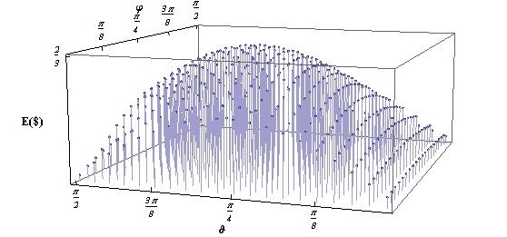
Figure 3: Expected payoff $E(\$(U^{\rm opt},\vartheta,\varphi))$ as a function of $\vartheta$ and $\varphi$, for a quantum KPR game with three players and three choices with the optimal strategy operator $U^{\rm opt}$. Each pair of $\vartheta$ and $\varphi$ indicates a different initial state according to Eq. (25). The peak in $E(\$)$ occurs for a maximally entangled initial state, i.e., for $\vartheta=\cos^{-1}(1/\sqrt{3})$ and $\varphi=\pi/4$ (taken from [36]).

4.2 Effect of decoherence

It is practically impossible to completely isolate a quantum system from the effects of the environment. Therefore, the studies that account for such effects have practical implications. In this context, the study of decoherence (or loss of phase information) is essential to understand the dynamics of a system in presence of system-environment interactions. Quantum games are recently being explored to implement quantum information processing in physical systems [37] and can be used to study the effect of decoherence in such systems [38, 39, 40, 41, 42]. In this connection, different damping channels can be used as a theoretical framework to study the influence of decoherence in quantum game problems.

We here study the effect of decoherence in three-player and three-choice quantum KPR problem by assuming different noise models, such as, amplitude damping, phase damping, depolarizing, phase flip and trit-phase flip channels, parameterized by a decoherence parameter $p$, where $p\in[0,1]$ [25]. The lower limit of decoherence parameter represents a completely coherent system, whereas the upper limit represents the zero coherence or fully decohered case.

In a noisy environment, the Kraus operator representation can be used to describe the evolution of a quantum state by considering the super-operator $\Phi$ [43]. Using density matrix representation, the evolution of the state is given by

$$\tilde{\rho}_{f}=\Phi(\rho_{f})=\sum_{k}E_{k}\rho_{f}E_{k}^{{\dagger}},$$ (27)

where the Kraus operators $E_{k}$ follow the completeness relation,

$$\sum_{k}E_{k}^{{\dagger}}E_{k}=I.$$ (28)

The Kraus operators for the game are constructed using the single qutrit Kraus operators as provided in Eqs. (30,31,32,33,34) by taking their tensor product over all $n^{3}$ combination of $\pi\left(i\right)$ indices

$$E_{k}=\underset{\pi}{\otimes}e_{\pi\left(i\right)},$$ (29)

with $n$ being the number of Kraus operators for a single qutrit channel. For the amplitude damping channel, the single qutrit Kraus operators are given by [44]

$$E_{0}=\left(\begin{array}[]{ccc}1&0&0\\ 0&\sqrt{1-p}&0\\ 0&0&\sqrt{1-p}\end{array}\right),\ \ E_{1}=\left(\begin{array}[]{ccc}0&\sqrt{p}&0\\ 0&0&0\\ 0&0&0\end{array}\right),\ \ E_{2}=\left(\begin{array}[]{ccc}0&0&\sqrt{p}\\ 0&0&0\\ 0&0&0\end{array}\right).$$ (30)

In a similar way, the single qutrit Kraus operators for the phase damping channel can be found as [35]

$$E_{0}=\sqrt{1-p}\left(\begin{array}[]{ccc}1&0&0\\ 0&1&0\\ 0&0&1\end{array}\right),\ \ E_{1}=\sqrt{p}\left(\begin{array}[]{ccc}1&0&0\\ 0&\omega&0\\ 0&0&\omega^{2}\end{array}\right),$$ (31)

where $\omega=e^{\frac{2\pi i}{3}}.$ For the depolarizing channel, the single qutrit Kraus operators take the forms as [20]

$$E_{0}=\sqrt{1-p}I,\ E_{1}=\sqrt{\frac{p}{8}}Y,\ E_{2}=\sqrt{\frac{p}{8}}Z,\ E_{3}=\sqrt{\frac{p}{8}}Y^{2},\ E_{4}=\sqrt{\frac{p}{8}}YZ,$$ (32)

$$E_{5}=\sqrt{\frac{p}{8}}Y^{2}Z,\ E_{6}=\sqrt{\frac{p}{8}}YZ^{2},\ \ E_{7}=\sqrt{\frac{p}{8}}Y^{2}Z^{2},\ \ E_{8}=\sqrt{\frac{p}{8}}Z^{2},$$ (33)

where

$$Y=\left(\begin{array}[]{ccc}0&1&0\\ 0&0&1\\ 1&0&0\end{array}\right),\ \ Z=\left(\begin{array}[]{ccc}1&0&0\\ 0&\omega&0\\ 0&0&\omega^{2}\end{array}\right).$$ (34)

The single qutrit Kraus operators, associated with the phase flip channel are given by

$$E_{0}=\left(\begin{array}[]{ccc}1&0&0\\ 0&\sqrt{1-p}&0\\ 0&0&\sqrt{1-p}\end{array}\right),\ \ E_{1}=\left(\begin{array}[]{ccc}0&\sqrt{p}&0\\ 0&0&0\\ 0&0&0\end{array}\right),\ \ E_{2}=\left(\begin{array}[]{ccc}0&0&\sqrt{p}\\ 0&0&0\\ 0&0&0\end{array}\right).$$ (35)

Similarly, the single qutrit Kraus operators for the trit-phase flip channel can be found as

$$E_{0} = \sqrt{1-\frac{2p}{3}}\left(\begin{array}[]{ccc}1&0&0\\ 0&1&0\\ 0&0&1\end{array}\right),\ \ E_{1}=\sqrt{\frac{p}{3}}\left(\begin{array}[]{ccc}0&0&e^{\frac{2\pi i}{3}}\\ 1&0&0\\ 0&e^{\frac{-2\pi i}{3}}&0\end{array}\right),$$ (42)

$$E_{2} = \sqrt{\frac{p}{3}}\left(\begin{array}[]{ccc}0&e^{\frac{-2\pi i}{3}}&0\\ 0&0&e^{\frac{2\pi i}{3}}\\ 1&0&0\end{array}\right),\ \ E_{3}=\sqrt{\frac{p}{3}}\left(\begin{array}[]{ccc}0&e^{\frac{2\pi i}{3}}&0\\ 0&0&e^{\frac{-2\pi i}{3}}\\ 1&0&0\end{array}\right),$$ (49)

where the term $p=1-e^{-\Gamma t}$ determines the strength of quantum noise which is usually called as decoherence parameter. This relation describes the bounds $[0,1]$ of $p$ by two extreme time limits $t=0$, $\infty$ respectively. The final density matrix representing the state after the action of the channel is given by

$$\tilde{\rho_{f}}=\Phi_{p}(\rho_{f})$$ (50)

where $\Phi_{p}$ is the super-operator for realizing a quantum channel parametrized by the decoherence parameter $p$. The payoff operator for $i^{\text{th}}$ player (say Alice) is given by Eq. (22).The expected payoff of $i^{\text{th}}$ player can be calculated as

$$E_{i}(\$)=\text{Tr}\{P_{A}\tilde{\rho}_{f}\}$$ (51)

where Tr represents the trace of the matrix. We have already studied the zero noise case ($p=0$) in Sec. 4 considering the fidelity $f=1$. It has been found that there exists an optimal unitary operator $U_{\rm opt}$ for which the expected payoff of a player becomes maximum. We here consider how a non-zero noise term $p$ and the fidelity, $f\neq 1$ affects the expected payoff.

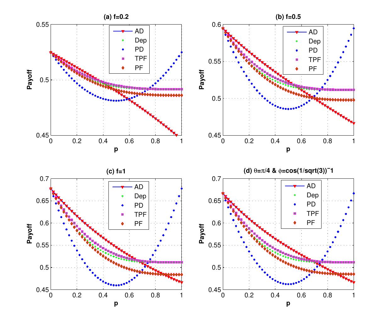
Figure 4: (Color online) Variation of Alice’s expected payoff as a function of the decoherence parameter $p$ for (a) $f=0.2,$ (b) $f=0.5,$ (c) $f=1$ and $\theta=\frac{\pi}{4},$ $\phi=\cos^{-1}(1/\sqrt{3})$ for amplitude damping, depolarizing, phase damping, trit-phase flip and phase flip channels (taken from [45]).

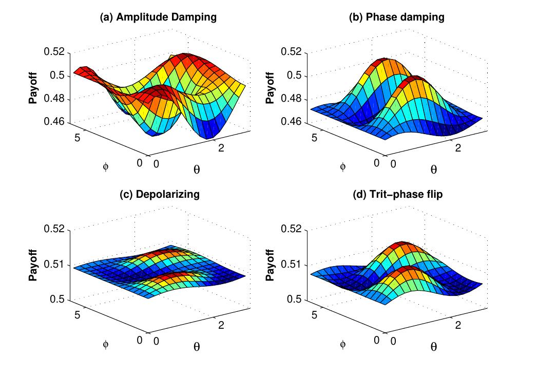
Figure 5: (Color online) Alice’s expected payoff as a function of $\theta$ and $\phi$ (determined by Eq. (25)) for (a) amplitude damping, (b) phase damping, (c) depolarizing and (d) trit-phase flip channels with decoherence parameter $p=0.7$ (taken from [45]).

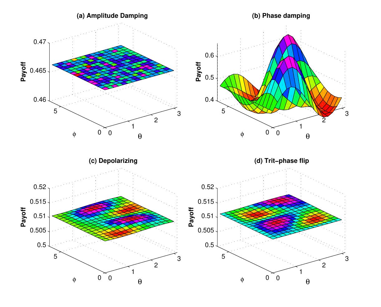
Figure 6: (Color online) Plot of Alice’s expected payoff as a function of $\theta$ and $\phi$ (determined by Eq. (25)) for (a) amplitude damping, (b) phase damping, (c) depolarizing and (d) trit-phase flip channels with decoherence parameter $p=1$ (from [45]).

In order to explain the effect of decoherence on the quantum KPR game, we investigate expected payoff by varying the decoherence parameter $p$ for different damping channels. Due to the symmetry of the problem, we have considered expected payoff of one of the three players (say Alice) for further investigations. In Fig. 4, the expected payoff of Alice is plotted as a function of decoherence parameter $p$ for different values of fidelity $f$ and different damping channels, such as, amplitude damping, depolarizing, phase damping, trit-phase flip and phase flip channels. It is observed that Alice’s payoff is strongly affected by the amplitude driving channel as compared to the flipping and depolarizing channels. The effect of entanglement of initial state is further investigated by plotting Alice’s expected payoff as a function of $\theta$ and $\phi$ in presence of noisy environment with decoherence parameter $p=0.7$ for different damping cases: (a) amplitude damping, (b) phase damping, (c) depolarizing and (d) trit-phase flip channels (see Fig. 5). In this scenario, one can see that Alice’s payoff is heavily affected by depolarizing noise compared to the other noise cases. This plot is also repeated for the highest level of decoherence, i.e., $p=1$ (see Fig. 6). It is seen that there is a considerable amount of reduction in Alice’s payoff for amplitude damping, deploarizing and trit-phase flip cases, whereas phase damping channel almost does not affect the payoff of Alice. Interestingly, the problem becomes noiseless for the maximum decoherence in the case of phase damping channel. Finally, the maximum payoff is achieved for the case of highest initial entanglement and zero noise, and it starts decreasing when the degree of entanglement deviates from maxima or introduces a non-zero decoherence term. Moreover, it has also been checked that the introduction of decoherence does not change the Nash equilibrium of the problem.

5 Summary and discussions

In the Kolkata Paise Restaurant or KPR game $\lambda N$ players choose every day independently but based on past experience or learning one of the $N~{}(\rightarrow~{}\infty)$ restaurants in the city. As mentioned, the game becomes trivial if a non-playing dictator prescribes the moves to each player. Because of iterative learning, the KPR game is not necessarily one-shot one, though for random choice (no memory or learning from the past) by the players.

For random choices of restaurants by the players, the game effectively becomes one-shot with convergence time $\tau=1$ and steady utilization fraction $f=1-exp(-\lambda)\simeq 0.63$ [8], as shown through Eqs. 1, 2, 3 of section 2. With iterative learning following Eq. 5a, 5b for $\lambda=1$, it was shown numerically, as well as with a crude approximation in [29], that the utilization fraction $f$ becomes of order $0.8$ within a couple of iterations ($\tau$ of the order of 10). In [31] the authors demonstrated numerically that for $\lambda=1$, $f$ can approach unity when $\alpha$ becomes $0_{+}$ from above. However the convergence time $\tau$ at this critical point diverges due to critical slowing down (see e.g., [6]), rendering such critically slow leaning of full utilization is hard to employ for practical purposes [46]. The cases of $\lambda<1$ (and $\alpha=1$) were considered earlier in [30]and [31], and has also been studied here in section 2, using Monte Carlo technique. A mean field-like transition (see e.g., [6]) is observed here giving full utilization ($f=1$) for $\lambda$ less than $\lambda_{c}$ about 0.75 where $\tau$ also remains finite. As shown in Fig. 1, $\tau$ diverges at the critical point $\lambda_{c}$ (a crude mean field derivation of it is given in Eq. 6).

For the quantum version of the KPR problem, we have discussed the one-shot game with three players and three choices that was first introduced in [23]; see also [27]. For this particular KPR game with three players and three choices, the classical randomization provides a total $27$ possible configurations, and $12$ out of them gives a payoff $\$=1$ to each of the players, thus leading to an expected payoff $E_{c}(\$)=4/9$. On the other hand, for the quantum case, it has been shown that when the players share a maximally entangled initial state, there exists a local unitary operation (same for all the players due to the symmetry of the problem) for which the players receive a maximum expected payoff $E_{q}(\$)=6/9$, i.e., the quantum players can increase their expected payoff by $50\%$ compared to their classical counterpart. To show the effect of entanglement, the expected payoff is calculated for a general GHZ-type initial state with different levels of entanglement (see Fig. 3). It appears that the maximally entangled initial state provides maximum payoff $E_{q}(\$)=6/9$ to each of the players. The expected payoff decreases from its maximum value for any deviation from the maximum entanglement of the initial state (see Fig. 3). This is the highest expected payoff that is attained so far for one-shot quantum KPR game with three players and three choices (see [24]). Until now, the study of the quantum KPR problem is limited to one shot with three players and three choices, and no attempt is found yet to make it iterative, and also to increase the number of players and choices. Therefore, it is yet to be understood whether one can increase the expected payoff by making the quantum KPR game iterative with learning from previous rounds as happened in the case of classical strategies studied here.

Decoherence is an unavoidable phenomenon for quantum systems, since it is not possible to completely isolate a system from the effects of the environment. Therefore, it is important to investigate the influence of decoherence on the payoffs of the players in the context of quantum games. The effect of decoherence in a three-player and three-choice quantum KPR problem is studied in [25] using different noise models like amplitude damping, phase damping, depolarizing, phase flip and trit-phase flip channels, parametrized by a decoherence parameter. The lower and upper limits of decoherence parameter represent the fully coherent and fully decohered system, respectively. Expected payoff is reported to be strongly affected by amplitude damping channel as compared to the flipping and depolarizing channels for lower level of decoherence, whereas it is heavily influenced by depolarizing noise in case of higher level of decoherence. However, for the case of highest level of decoherence, amplitude damping channel dominates over the depolarizing and flipping channels, and the phase damping channel has nearly no effect on the payoff. Importantly, the Nash equilibrium of the problem is shown not to be changed under decoherence.

There have been several applications of KPR game strategies to various social optimization cases. KPR game has been extended to Vehicle for Hire Problem in [10, 11]. Authors have built several model variants such as Individual Preferences, Mixed Preferences, Individual Preferences with Multiple Customers per District, Mixed Preferences and Multiple Customers per District, etc.. Using these variants, authors have studied various strategies for the KPR problem that led to a foundation of incentive scheme for dynamic matching in mobility markets. Also in [11], a modest level of randomization in choice along with mixed strategies is shown to achieve around 80% of efficiency in vehicle for hire markets. A time-varying location specific resource allocation crowdsourced transportation is studied using the methodology of mean field equilibrium [47]. This study provides a detailed mean field analysis of the KPR game and also considers the implications of an additional reward function. In [12], a resource allocation problem for large Internet-of-Things (IoT) system, consisting of IoT devices with imperfect knowledge, is formulated using the KPR game strategies. The solution, where those IoT devices autonomously learn equilibrium strategies to optimize their transmission, is shown to coincides with the Nash equilibrium. Also, several ‘emergent properties’ of the KPR game, such as the utilization fraction or the occupation density in the steady or stable states, phase transition behavior, etc., have been numerically studied in [48]. A search problem often arises as a time-limited business opportunity by business firms, and is studied like an one-shot delegated search in [49]. Authors here had discussed and investigated the searchers’ incentives following different strategies, including KPR, that can maximize the search success. Authors in [13] have discussed KPR problem as Traveling Salesman Problem (TSP) assuming restaurants are uniformly distributed on a two-dimensional plane and this topological layout of the restaurants can help provide each agent a second chance for choosing a better or less crowded restaurant. And they have proposed a meta-heuristics, producing near-optimal solutions in finite time (as exact solutions of the TSP are prohibitively expensive). Thus agents are shown to learn fast, even incorporating their own preferences, and achieves maximum social utilization in lesser time with multiple chances.

References

- [1] O. Morgenstern and J. Von Neumann. Theory of games and economic behavior. Princeton university press (1953).
- [2] Prisoner’s Dilemma. The Stanford encyclopedia of philosophy. https://plato.stanford.edu/entries/prisoner-dilemma/ (2019).
- [3] M. J. Osborne and A. Rubinstein. A course in Game theory. MIT press (1994).
- [4] B. Lockwood. Pareto Efficiency, The New Palgrave Dictionary of Economics (2nd ed.). Palgram Macmillan, pages 292-294 (2008).
- [5] D. Challet, M. Marsili, and Y.-C. Zhang. Minority Games: Interacting agents in financial markets. Oxford University Press (2005).
- [6] H. E. Stanley. Introduction to Phase Transitions and Critical Phenomena. Oxford University Press (1987).
- [7] B. K. Chakrabarti. Kolkata restaurant problem as a generalised el farol bar problem. In Econophysics of Markets and Business Networks, pages 239–246. Springer (2007).
- [8] A. S. Chakrabarti, B. K. Chakrabarti, A. Chatterjee, et al. The Kolkata Paise Restaurant problem and resource utilization. Physica A: Statistical Mechanics and its Applications, 388, 2420 (2009).
- [9] B. K. Chakrabarti, A. Chatterjee, A. Ghosh, et al. Econophysics of the Kolkata Restaurant Problem and Related Games: Classical and Quantum Strategies for Multi-agent, Multi-choice Repetitive Games. New Economic Windows, Springer (2017).
- [10] L. Martin. Extending Kolkata Paise Restaurant problem to dynamic matching in mobility markets. Junior Management Science, 4, 1 (2017). https://jums.ub.uni-muenchen.de/JMS/article/view/5032/3210.
- [11] L. Martin and P. Karaenke. The vehicle for hire problem: A generalized Kolkata Paise Restaurant problem. In Workshop on Information Technology and Systems (2017). https://mediatum.ub.tum.de/doc/1437330/1437330.pdf.
- [12] T. Park and W. Saad. Kolkata paise restaurant game for resource allocation in the Internet of Things. In 2017 51st Asilomar Conference on Signals, Systems, and Computers, pages 1774–1778. IEEE (2017). https://ieeexplore.ieee.org/document/8335666.
- [13] K. Kastampolidou, C. Papalitsas, and T. Andronikos. DKPRG or how to succeed in the kolkata paise restaurant game via TSP (2021). https://arxiv.org/pdf/2101.07760.pdf.
- [14] D. A. Meyer. Quantum strategies. Physical Review Letters, 82, 1052 (1999).
- [15] J. Eisert, M. Wilkens, and M. Lewenstein. Quantum games and quantum strategies. Physical Review Letters, 83, 3077 (1999).
- [16] S. C. Benjamin and P. M. Hayden. Multiplayer quantum games. Physical Review A, 64, 030301 (2001).
- [17] L. Marinatto and T. Weber. A quantum approach to static games of complete information. Physics Letters A, 272, 291 (2000).
- [18] E. W. Piotrowski and J. Sładkowski. An invitation to quantum game theory. International Journal of Theoretical Physics, 42, 1089 (2003).
- [19] S. A. Bleiler. A formalism for quantum games and an application (2008). https://arxiv.org/pdf/0808.1389.pdf.
- [20] S. Salimi and M. Soltanzadeh. Investigation of quantum roulette. International Journal of Quantum Information, 7, 615 (2009).
- [21] S. E. Landsburg. arXiv, 1110.6237 (2011). https://arxiv.org/pdf/1110.6237v1.pdf.
- [22] Q. Chen, Y. Wang, J.-T. Liu, et al. N-player quantum minority game. Physics Letters A, 327, 98 (2004).
- [23] P. Sharif and H. Heydari. Quantum solution to a three player Kolkata restaurant problem using entangled qutrits (2011). https://arxiv.org/pdf/1111.1962.pdf.
- [24] P. Sharif and H. Heydari. Strategies in a symmetric quantum Kolkata restaurant problem. In AIP Conference Proceedings, volume 1508, pages 492–496. American Institute of Physics (2012). http://citeseerx.ist.psu.edu/viewdoc/download?doi=10.1.1.752.7777&rep=rep1&type=pdf.
- [25] M. Ramzan. Three-player quantum Kolkata restaurant problem under decoherence. Quantum information processing, 12, 577 (2013).
- [26] P. Sharif and H. Heydari. An introduction to multi-player, multi-choice quantum games: Quantum minority games & kolkata restaurant problems. In Econophysics of Systemic Risk and Network Dynamics, pages 217–236. Springer (2013).
- [27] P. Sharif and H. Heydari. An introduction to multi-player, multi-choice quantum games (2012). https://arxiv.org/pdf/1204.0661.pdf.
- [28] A. Ghosh, A. S. Chakrabarti, and B. K. Chakrabarti. Kolkata Paise Restaurant problem in some uniform learning strategy limits. In Econophysics and Economics of Games, Social Choices and Quantitative Techniques, pages 3–9. Springer (2010).
- [29] A. Ghosh, A. Chatterjee, M. Mitra, et al. Statistics of the kolkata paise restaurant problem. New Journal of Physics, 12, 075033 (2010).
- [30] A. Ghosh, D. De Martino, A. Chatterjee, et al. Phase transitions in crowd dynamics of resource allocation. Physical Review E, 85, 021116 (2012).
- [31] A. Sinha and B. K. Chakrabarti. Phase transition in the Kolkata Paise Restaurant problem. Chaos: An Interdisciplinary Journal of Nonlinear Science, 30, 083116 (2020).
- [32] B. K. Chakrabarti and A. Sinha. Development of Econophysics: A Biased Account and Perspective from Kolkata. Entropy, 23, 254 (2021).
- [33] M. Mathur and D. Sen. Coherent states for SU (3). Journal of Mathematical Physics, 42, 4181 (2001).
- [34] C. Schmid, A. P. Flitney, W. Wieczorek, et al. Experimental implementation of a four-player quantum game. New Journal of Physics, 12, 063031 (2010).
- [35] M. Ramzan and M. Khan. Decoherence and entanglement degradation of a qubit-qutrit system in non-inertial frames. Quantum Information Processing, 11, 443 (2012).
- [36] P. Sharif and H. Heydari. arXiv, 1212.6727 (2012). https://arxiv.org/pdf/:1212.6727.
- [37] I. Pakuła. Quantum gambling using mesoscopic ring qubits. physica status solidi (b), 244, 2513 (2007).
- [38] A. P. Flitney and D. Abbott. Quantum games with decoherence. Journal of Physics A: Mathematical and General, 38, 449 (2004).
- [39] N. F. Johnson. Playing a quantum game with a corrupted source. Physical Review A, 63, 020302 (2001).
- [40] M. Ramzan and M. Khan. Noise effects in a three-player prisoner’s dilemma quantum game. Journal of Physics A: Mathematical and Theoretical, 41, 435302 (2008).
- [41] L. Chen, H. Ang, D. Kiang, et al. Quantum prisoner dilemma under decoherence. Physics Letters A, 316, 317 (2003).
- [42] M. Ramzan and M. Khan. Distinguishing quantum channels via magic squares game. Quantum Information Processing, 9, 667 (2010).
- [43] M. A. Nielsen and I. L. Chuang. Quantum computation and quantum information. Physics Today, 54, 60 (2001).
- [44] K. Ann and G. Jaeger. Finite-time destruction of entanglement and non-locality by environmental influences. Foundations of Physics, 39, 790 (2009).
- [45] M. Ramzan. arXiv, 1111.3913 (2011). https://arxiv.org/pdf/1111.3913.pdf.
- [46] M. San Miguel and R. Toral. Introduction to the chaos focus issue on the dynamics of social systems (2020).
- [47] P. Yang, K. Iyer, and P. Frazier. Mean field equilibria for resource competition in spatial settings. Stochastic Systems, 8, 307 (2018).
- [48] B. Tamir. Econophysics and the Kolkata Paise Restaurant Problem: More is different. Science & Culture, 84, 37 (2018). https://www.scienceandculture-isna.org/jan-feb-2018/05%20Art_Econophysics_and_the_Kolkata_Paise...by_Boaz%20Tamir_Pg.37.pdf.
- [49] R. Hassin. Equilibrium and optimal one-shot delegated search. IISE Transactions, 53, 928 (2021). DOI:10.1080/24725854.2019.1663085.