Sparse Subspace Clustering for Concept Discovery (SSCCD)

Abstract

Concepts are key building blocks of higher level human understanding. Explainable AI (XAI) methods have shown tremendous progress in recent years, however, local attribution methods do not allow to identify coherent model behavior across samples and therefore miss this essential component. In this work, we study concept-based explanations and put forward a new definition of concepts as low-dimensional subspaces of hidden feature layers. We novelly apply sparse subspace clustering to discover these concept subspaces. Moving forward, we derive insights from concept subspaces in terms of localized input (concept) maps, show how to quantify concept relevances and lastly, evaluate similarities and transferability between concepts. We empirically demonstrate the soundness of the proposed Sparse Subspace Clustering for Concept Discovery (SSCCD) method for a variety of different image classification tasks. This approach allows for deeper insights into the actual model behavior that would remain hidden from conventional input-level heatmaps.

1 Introduction

In neuroscience, concepts are defined as flexible, distributed representations comprised of modality-specific conceptual features and are important building blocks of human cognition [1]. Like neuroscience sheds light on human mental processes, the subfield of Explainable AI in machine learning develops methods that provide insights into the decision processes in particular inside deep neural networks, see [2, 3, 4, 5] for reviews.

Here, we are concerned with local interpretability methods that provide attributions for individual samples, which is desirable for most applications. However, to acquire a higher-level understanding of the model, the user needs to aggregate numerous samples into a common explanation. Not only is the human ability for this limited, but the summarization is also prone to human confirmation bias [6]. Even leaving these issues aside, the resulting insights do not reflect the actual reasoning structure hidden for example in the feature layers of a model. This urges for novel local and concept-based interpretability methods, that explore shared structures in the decision process of the neural network across several examples. We stress already at this point that our primary motivation is to reveal coherent, discriminative structures exploited by the model rather than achieving best accordance with concepts identified by humans.

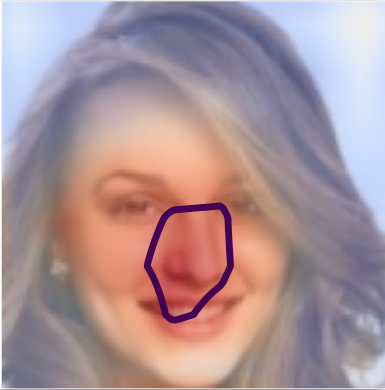
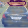
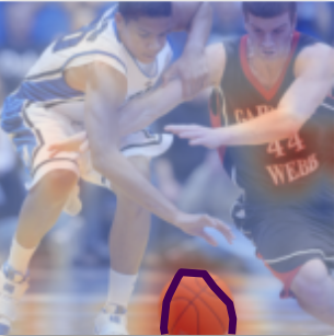
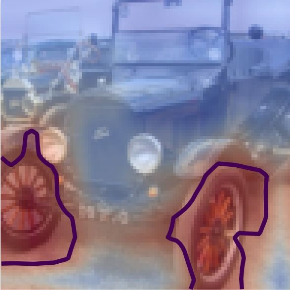
ResNet50	ResNet50	VGG16	VGG16
CelebA	ImageNet	ImageNet	ImageNet

Figure 1: SSCCD successfully discovers concepts for a variety of datasets and models.

The common aspect of exisiting concept-based interpretability methods, such as [7, 6, 8], is the fact that they understand concepts as single vectors in the space of intermediate hidden feature layers and are in this sense meaningful to the model. It lies in the nature of a concept as an abstract representation that its expressions can be diverse. Therefore, it is surprising that the definition of concepts as one-dimensional feature subspaces has so far not been challenged. We novelly argue for concepts as low-dimensional subspaces. Multiple feature dimensions enable to fully capture the intra-concept diversity described above (benefit 1). To discover these low-dimensional concept subspaces in feature space we build on the successful application of sparse subspace clustering in input space [9]. The approach stands out from many of its competitors as it does not require reinforcing the interpretability of concepts (e.g. through prior superpixel segmentation, regularizer to enforce the dissimilarity of concepts etc. ) and thus reflects the inner workings of the model as faithfully as possible (benefit 2). Additionally, we characterize the identified concept subspaces by a basis and propose similarity measures between them. In contrast to generic, untargeted concepts for the whole classifier, our approach allows extracting class-specific concepts, as well as concepts based on specific combinations of classes. Altogether, this enables a quantitative comparison of concepts, the transferability to different classes, and thus a comprehensive model understanding.

Every concept interpretability method comes with a number of sub-components: (a) concept discovery (b) mapping from feature space to input space (c) relevance quantification. We stress at this point that any concept interpretability method has to decide on these sub components either explicitly or implicitly. As mentioned above, we see an appropriately modified sparse subspace clustering as an ideal fit for the identification of concept subspaces (a). For (b), we follow [10] and translate feature level concept maps to the input level by simple bilinear interpolation. In our view, alternative mappings, which are usually based on receptive fields, often overestimate the area of impact. Finally, concerning (c), we put forward a framework that allows inferring the concept relevance with any interpretability method either anchored in input or feature space. This leads to a robust method that works across different datasets and model architectures, see Figure 1. To summarize, our main contributions are the following:

• Novel concept definition as low-dimensional feature subspaces

• Sparse subspace clustering for concept discovery

• Relevance quantification for concepts via user-defined attribution method

• Insights from a quantitative similarity measure between concept subspaces

2 Sparse Subspace Clustering for Concept Discovery (SSCCD)

We start by motivating our definition of concepts which form the building blocks of a deep neural network’s reasoning process. For definiteness, we focus on convolutional neural networks (CNN) in this section and comment on extensions to other architectures below. Our approach is based on the following principles, which align with the aspects put forward in the introduction:

(1) Concepts should be meaningful to the model, i.e. should be inherently tied to hidden feature layers to ensure that the concepts correspond to intermediate processing steps within the network. (2) Concepts should allow to capture the intra-concept diversity that is inherent to the typically abstract nature of concepts. In this work, we argue that the until now uncontested definition [7, 6, 8] of concepts as single directions, i.e. one-dimensional feature subspaces is generally not enough and postulate to define concepts as linear subspaces in feature space. For practical considerations, we require these subspaces to be robust against noise and outliers.

In addition, we believe that there are further desirable properties that a concept discovery framework (CDF) should satisfy:

(3) A CDF should allow to spatially localize the concept in feature or input space, see the discussion on concept maps below, whereas the definition of the concept itself should not explicitly make reference to the spatial location within the feature layer. (4) A CDF should provide a relevance quantification of a concept in terms of its impact on the classification decision. (5) A CDF should allow to assess the similarity between different concepts, both within and across different classes. Given a sensible concept definition, concepts should be transferable between samples from semantically similar classes.

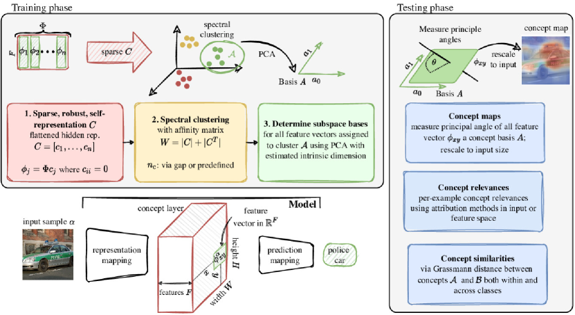
Figure 2: Schematic illustration of the SSCCD-approach for concept discovery.

Concept definition

As a first step, we select a set of samples $S$, for which we aim to discover concepts. We pose no restrictions on the samples in $S$, i.e. the user can decide for class-specific samples/concepts or up to all training samples to obtain completely class-unspecific concepts. Our definition is then based on the hidden representations $h(\alpha\in\mathbb{R}^{H\times W\times F})$ of input samples $\alpha\in S$ with width (of the feature layer) $H$, height $W$ and number of features $F$. We spatially deconstruct the feature maps $h(\alpha)$ and obtain a feature vector $\phi^{\alpha}_{xy}\in\mathbb{R}^{F}$ for each location $(x,y)\in\{1,\ldots,H\}\times\{1,\ldots,W\}$. We define a concept as a robust subspace of the $F$-dimensional feature space.

Note that this definition does not include any constraints on the spatial coherence of concepts nor does it include additional constraints such as penalizing similar clusters as in [8]. In this way, the concept discovery process does not obfuscate the structures the model is exploiting. Concepts are as true to the model as possible (benefit 2). To identify concept subspaces we draw on the rich body of literature on sparse subspace clustering (SSC) [9, 11, 12, 13]. As nicely laid out in [9], SSC is ideally suited to identify clusters of linear subspaces and provides a number of advantages over standard clustering algorithms, which are directly applied to the data: SSC does not take advantage of the spatial proximity of the data e.g. to characterize clusters via a centroid, it can be implemented robustly against noise and outliers and does not require to specify the different cluster dimensionalities in advance. In the following, we describe our method, which we split into training and test phase.

2.1 Training: Concept discovery

During training, concepts are discovered through the Sparse Subspace Clustering for Concepts Discovery (SSCCD) procedure, see also Figure 2 for a schematic representation:

1. Concept-determining self-representation

We compute sparse self-representations $C$ for a random sub-collection of $n\leq N\cdot H\cdot W$ feature vectors $\{\phi^{\alpha}_{xy}\}$ sampled from $S$. Here, the term self-representation refers to a coefficient matrix that expresses each sample as a linear combination of all other samples. More specifically, using the notation from [9], given the feature vectors $\Phi=[\phi_{1},\ldots,\phi_{n}]\in\mathbb{R}^{F\times n}$, we identify a sparse coefficient matrix $C=[c_{1},\ldots,c_{n}]\in\mathbb{R}^{n\times n}$ such that

$$\phi_{j}=\Phi c_{j}\,\,\text{where}\,\,c_{ii}=0.$$ (1)

The particular kind of sparsity constraints that are imposed on Equation 1 and how it is optimized depends on the chosen SSC algorithm. Here, we use elastic net subspace clustering [13], which is robust against noise and scales well for large sample sizes. In all our experiments, we fix the hyperparameter $\gamma$, which balances sparsity vs. robustness, to $\gamma=10$.

We remove outliers based on the $\ell_{1}$-norm as in [11], where we empirically fix the percentile threshold to 0.75 and re-fit the sparse self-representation for the remaining elements. Another scalable alternative to the elastic net clustering is orthogonal matching pursuit (OMP)[12], which is, however, not robust against noise and does not allow for outlier removal via thresholding. Finally, the original sparse subspace clustering method from [9] is robust against noise and outliers but does not scale to large datasets. The particular robustness and scalability properties make elastic net subspace (with thresholding) an ideal choice for the first step of our concept discovery method.

2. Spectral clustering

We perform spectral clustering with the affinity matrix $W=|C|+|C^{T}|$, which encodes the similarity of two feature vectors according to their self-representations. We determine the number of clusters $n_{c}$ either via the largest gap in the spectrum of the Laplacian [14] or use a predetermined value. This step assigns every input feature $\phi_{i}$ to a particular cluster $\mathcal{C}_{1},\ldots,\mathcal{C}_{n_{c}}$ or to the set of outliers.

3. Identifying subspace basis elements

Next, we turn to the identified concepts, which are defined via the corresponding cluster members, and construct a low-dimensional basis as we aim to characterize concepts via subspaces rather than cluster members. Concretely, for a given cluster $\mathcal{A}$, we aim to identify a basis $A$ that robustly covers $\mathcal{A}$. To this end, we apply principal component analysis (PCA) and determine the intrinsic dimension of the subspace using a heuristic proposed by [15] as implemented in [16]. The PCA components up to the intrinsic dimension then serve as a basis for the subspace $A$.

We stress that the overall methodology is applicable beyond CNNs. In particular, one can decompose feature representations of any model based on SSCCD. However, human identification of the identified concept subspaces requires the ability to connect spatial locations in the feature layer with spatial locations in the input space. Due to the local nature of convolutions, this can be achieved by upsampling the spatial dimensions, as described for concept maps below. Clearly localized attention maps [17] show that locality is induced via skip-connections in transformer architectures.

2.2 Test: Insights from concept subspaces

To test the discovered concepts, we evaluate how the model employs them to classify (new and unseen) samples. We visualize where the model identified a concept in input space by concept (expression) maps and quantify its relevance towards the prediction. Additionally, we quantify the relation between concept subspaces based on a measure for concept similarities. The central tool here are principal angles $\theta_{i}^{AB}$ [18] ($i=1,\ldots,\min(\text{dim}\,A,\text{dim}\,B)$) between two linear subspaces, which are defined recursively via

$$\cos\theta_{i}^{AB}=\underset{a\in A,b\in B}{\max}\tfrac{a^{T}b}{\left\lVert a\right\rVert_{\ell_{2}}\left\lVert b\right\rVert_{\ell_{2}}}=:\tfrac{a_{i}^{T}b_{i}}{\left\lVert a_{i}\right\rVert_{\ell_{2}}\left\lVert b_{i}\right\rVert_{\ell_{2}}}\,,$$ (2)

where the maximum is taken subject to the orthogonality constraints $a^{T}a_{j}=0$ and $b^{T}b_{j}=0$ for $j=1,\ldots,i-1$.

Concept (expression) maps

We can use the principal angle $\theta_{1}^{\phi^{\alpha}_{xy}A}$ to characterize the relation between a feature vector $\phi^{\alpha}_{xy}$ (i.e. a one-dimensional subspace) of the $\alpha$-sample and a concept $\mathcal{A}$. If we apply this across all spatial dimensions $(x,y)$, we can define a concept map that spatially resolves the similarity of the feature layer $\phi^{\alpha}_{xy}$ to the concept, i.e. $\theta^{\alpha A}_{xy}:=\theta^{\phi^{\alpha}_{xy}A}_{1}$. Here, high similarity (i.e. highly activated concepts) corresponds to a small principal angle $\theta^{\alpha A}_{xy}$. Due to the local nature of convolutional layers, we next leverage bilinear upsampling to resize the concept map to the input image size. This enables to represent the meaning of concepts in input space and allows to overlay images with color-coded concept maps. To guide the eye, we include contour lines that are defined via the median of all principal angles belonging to a particular concept, i.e. we define a concept-specific threshold angle via $\delta^{A}=\text{Median}(\{\theta_{1}^{\phi A}|\phi\in\mathcal{A}\})$. More precisely, the median is taken with respect to all features vectors which belong to a particular cluster $\mathcal{A}$ during the concept discovery step 1. This provides a way of obtaining hard concept assignments in input or feature space without the necessity of introducing an additional hyperparameter. Finally, we can define a sample-concept proximity measure $\delta^{\alpha A}=\text{min}_{xy}(\theta^{\alpha A}_{xy})$ as the minimal principle angle between a concept subspace $A$ and all feature vectors of the $\alpha$-sample.

Concept relevances

Finally, we are not only interested in the discovery of concepts as specific structures in the model’s feature space, but moreover, we also desire to quantify the concept’s relevance for the classification decision on a per-example basis. For SSCCD this can be achieved by an attribution method either based in input or feature space.

To this end, we use the threshold angles defined above to convert concept maps into binary masks to identify regions in input/feature space that are associated with a particular concept. Then the relevance of these concept masks can be quantified using an established attribution methods. As an advantage, our novel SSCCD-approach can be combined with any attribution method in input space or alternatively directly in the feature space. For definiteness, we consider PredDiff [19, 20] and Integrated Gradients [21] in this work. In the case of Integrated Gradients, we sum up the individual pixel relevances, in contrast for PredDiff, we directly obtain superpixels attributions. Like [22] we first evaluate instance-wise relevance scores and later aggregate these to class-wise concept relevance.

Concept similarities

To quantitatively characterize the similarity between two concepts $\mathcal{A}$ and $\mathcal{B}$, we use their Grassmann distance [23], which is defined as $d^{AB}=\sqrt{(\theta_{1}^{AB})^{2}+\ldots+(\theta_{\text{min}(\text{dim}\,A,\text{dim}\,B)}^{AB})^{2}}$. This allows comparing the similarity of concepts within a given class or across classes regardless of the concept subspaces’ dimensionality.

3 Related Work

ACE [7] uses a superpixel segmentation algorithm and $k$-means clustering to identify class-specific concept candidates for TCAV [6].

The concept discovery scheme of ACE has several shortcomings: The segmentation, i.e. the candidate concept patches, is model-independent and thus segments are not necessarily meaningful as perceived by the model.

To enable clustering of intermediate CNN activations, segments are resized and mean padded to the original input shape. This leads to artificial, off-manifold samples with potentially distorted aspect ratios and discards the overall scale information.

Finally, ACE relies on multiple heuristics to discard segments/clusters both before and after $k$-means clustering. In contrast, spectral clustering in SSCCD is coherently based on hidden model representations without relying on additional pre- or postprocessing. Similar limitations apply to methods that rely on ACE-discovered labeled concepts, like [22], which uses Shapley values for concept importance, and [24], which occludes particular neurons for neuron-wise relevances and transforms them into concept importances via concept classification.

ICE [25] defines concepts as directions in feature space. Technically, this is achieved via dimensionality reduction techniques applied to concatenated flattened feature maps. ICE measures the importance of its class-wise concepts using TCAV. Other methods learn concept vectors and a mapping to feature space either for all classes simultaneously (ConceptSHAP [8]) or for each class separate (MACE [26], PACE [27]). Importantly, each method defines a custom measure for concept importance which is only applicable within the respective framework. All these concept importance measures are based on approximations of the original model. In contrast, SSCCD can build on any (established) attribution method both in input or feature space. Our results indicate that concepts are multi-dimensional in feature space. ConceptShap, MACE and PACE need to account for this via additional regularizers enforcing dissimilarity. SSCCD in comparison can identify diverse concept subspaces in a fully unsupervised way.

There is a complementary line of work where one tries to analyze CNN hidden representations in combination with special concept-annotated datasets. Network Dissection [28] investigates the alignment of human-understandable concepts and particular single hidden features (neurons). [29] extended this by allowing concepts to be represented by combinations of neurons. Alternatively, [30] projects model representations onto an interpretable basis, which is learned from a pixel-level segmented and annotated dataset.

4 Results

We limit our experiments to natural images and CNNs and defer extensions to other datasets and architectures to future work. We use two popular, large-scale image recognition datasets, ImageNet[31] and the CelebFaces Attributes Dataset (CelebA) [32]. As for ImageNet, we use pretrained VGG16 [33] and ResNet50 [34] model as provided by torchvision. On CelebA, we train a ResNet50 model from scratch on the full set of 40 attributes using a binary crossentropy loss. The model reaches a macro AUC of 0.92 on the CelebA test set.

In the following, we showcase the abilities of SSCCD for the different datasets and model architectures and derive a number of new insights from them. We stress already at this point that all presented results are strictly based on test set samples whereas the concepts itself are discovered on the training dataset.

Our main analysis tool for qualitative assessment of the discovered concepts are concept maps. In the following, the rows of all concept maps, e.g. Figure 3, are sorted according to their average concept relevances. Here, we used Integrated Gradients to obtain attributions and calculate the per-sample concept relevances via summing all attributions over the thresholded (red) regions of the concept maps in input space. We further assessed the effect of this relevance quantification method. Firstly, we replaced Integrated Gradients with PredDiff and secondly, measure attributions in feature space directly (for both methods), see supplementary material for details. It reassuring that, despite differences in the numerical values, the concept ranking based on these importances is largely consistent across all methods. Lastly, we used a predefined number of five concepts for all of the following experiments.

4.1 Impact of multi-dimensionality

First, we investigate the advantage of multidimensional concept subspaces as given by SSCCD’s concept definition (benefit 1) over concept vectors, i.e. one-dimensional subspaces, used in the literature. If one restricts to one-dimensional concept vectors only, a different concept discovery method is appropriate. Straightforward candidates are dimensionality reduction methods such as PCA or NNMF, which are directly applied in feature space.

high intra-class variance			low intra-class variance
SSCCD	PCA/ICE-baseline		SSCCD	PCA/ICE-baseline

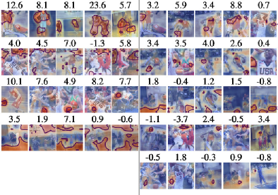
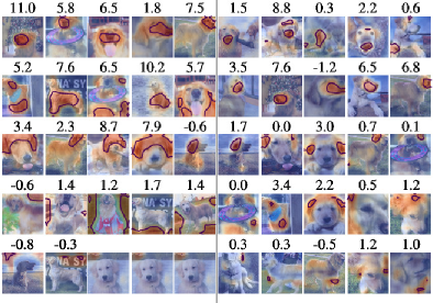
Figure 3: Concept maps for basketball class (left) and golden retriever class (right) and a VGG16 model (final convolutional layer). For concept maps, red regions denote high concept proximity and lines indicate the concept-dependent thresholds $\delta^{A}$. We compare multi-dimensional SSCCD concepts to one-dimensional concepts obtained via direct application of PCA in feature space as used by ICE [25]. The fifth SSCCD concept of the basketball class was not activated (below threshold) on the whole test set and was therefore omitted. Subtitles indicate the per-sample concept relevances (via Integrated Gradients in input space). Rows are sorted by average concept relevance and the closest proximity samples are shown.

In Figure 3, we compare SSCCD concept maps to those obtained from applying PCA directly in feature space, which corresponds to one of the concept discovery methods used by ICE [25]. Different from ICE, we choose a threshold relative to the maximum sample-concept proximity per concept across all training samples, using a factor of $1.2$, for the PCA approach. This corresponds to $\delta^{A}$ for SSCCD. We focus on the basketball class and the golden retriever class as examples with high and low intra-class variance, respectively, see the supplementary material for further class examples. Samples from a class with high intra-class variance are more diverse than samples from a class with low intra-class variance. The resulting basketball concepts demonstrate the shortcomings of the one-dimensional PCA approach. SSCCD concepts are clearly localized and identifiable (shirt, heads, ball, gym floor/wall). In contrast, PCA basketball concepts are less localized and often incoherent. In particular, the ball itself is not even recognized as a concept. For diverse (but coherent) concepts such as colorful shirts or backgrounds, the PCA approach is forced to create separate concept vectors. SSCCD, however, can account for this via a common multidimensional concept subspace, which demonstrates benefit 1. In accordance with expectations, the PCA approach tends to show most satisfying results for the simpler golden retriever class where samples and hence concept expressions are more uniform than for the basketball class. Still, the PCA approach identifies two separate directions for the nose concept.

4.2 Dependence on model architecture

VGG16                         ResNet50

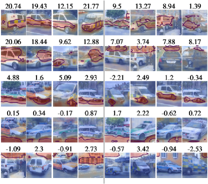
Figure 4: SSCCD concept maps with per-sample concept relevances (via Integrated Gradients in input space) for the police van class from ImageNet. Each row corresponds to a different concept sorted by average concept relevance. For easier concept identification, we show samples with the smallest sample-concept proximity. Random selections are presented in the supplementary material. VGG16: last feature layer in the last block. ResNet50: last feature layer in the second-last block.

To demonstrate that the approach is applicable irrespective of the particular model architecture, we show concepts for a VGG16 and a ResNet50 model in Figure 4, where we specialize to the police car class. We defer the reader to the supplementary material for alternative ImageNet classes. For comparability, both feature layers in Figure 4 were chosen such that they have the equal spatial size $14\times 14$. Alternative feature layer choices are presented in the supplementary material.

For VGG16, SSCCD identifies livery (8.0), windows (7.8), tires/underbody (3.7), street (0.5), buildings (0.3) as most important concepts. Here, values in brackets denote the average concept relevance as measured on all test samples. For a ResNet50 model we obtain livery/windows (5.4), emergency lights (3.1), tires/ underbody (1.2), street (0.3), sky/background (0.02) as most relevant concepts. Interestingly, both models identify similar concepts and also their ranking, based on concept relevances, agrees. For ResNet50, the secondly ranked concept of emergency lights stands out, as it was not identified among the VGG concepts. This provides a hint towards different strategies followed by the two networks. Importantly, such insights are hard to obtain via raw attribution-based explanation strategies. Note further, that in both cases also typical background structures were identified as coherent concepts. However, these concepts are not informative for the classification task and consequently assigned a comparable low average concept relevance.

4.3 Insights: class vs. anti-class concepts

The CelebA dataset with its 40 binary attributes represents an ideal test bed to investigate the behavior of concepts for (anti-)class (where a particular attribute is either present or absent) samples. For definiteness, we demonstrate this behavior for the “male” attribute and refer the reader to the supplementary material for further attributes. This experiment provides a perfect example for unique insights that can solely be gained from concept-based methods, which for example reveal the subtle difference between female and male nose concepts (see below). Importantly, these insights would remain hidden for standard local attribution methods (which would only highlight the nose region in both cases).

The left panel of Figure 5 shows the most important male concepts exploited by the model. These can be tagged as chin (1.1), nose (1.0), hair(line) (0.5) as well as two (irrelevant) background concepts ($-$0.3, $-$0.8), where values in brackets denote the average concept relevance. This, in combination with similar findings for further attributes presented in the supplementary material, entails that the number of discriminative concepts is rather small, which seems plausible given the homogeneity of the dataset and the rather simple binary classification tasks. Not surprisingly, the male concepts mostly activate for the corresponding regions in the female face, when evaluated on female samples. However, for the non-background concepts, concept proximities barely reach values below the respective concept activation threshold. We quantify this statement by measuring their average normalized sample-concept proximity scores across the whole dataset, $\delta^{\alpha A}/\delta^{A}$, where $\delta^{A}$ is the activation threshold. Values larger than one indicate that the concept is on average not activated. We find (0.95, 0.99, 0.98) for male and (0.99, 1.05, 1.01) for female samples. Thus, only the male chin concept is activated on the female samples by a small margin whereas both nose and hair concepts remain unactivated. In the right panel of Figure 5, we visualize female concepts, which interestingly show a slightly differently localized chin/hair concept as most important concept. To summarize, the identified concepts are highly specific both in terms of localization (c.f. chin for “male” vs. neck/hair for “female”) and in terms of underlying features. The latter can be inferred from the fact that similarly localized concepts (e.g. nose for “male”/“female”, hair for “young”/“old”, see the supplementary material) are found for class and anti-class but evaluating a particular concept only weakly activates the corresponding region with the anti-concept. As a final remark, we envision that SSCCD can be used as a detection tool for model biases (e.g. gender or race-related). This would entail comparing concepts discovered from a biased selection of samples to a balanced selection of samples.

male concepts			female concepts
male samples	female samples		female samples	male samples

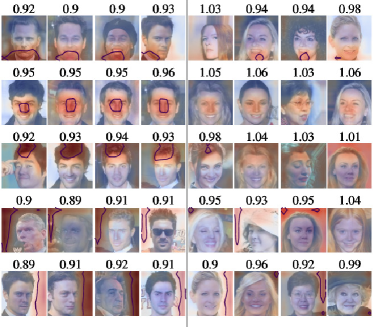
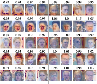
Figure 5: SSCCD concepts on CelebA for a ResNet50 model for samples with the “male” (left) and “female” (right) attribute. Concepts are ordered according to average concept relevance showing samples with smallest sample-concept proximity. We apply the same male concept on a random selection of female samples and vice-versa. Subtitles indicate the normalized sample-concept proximity $\delta^{iA}/\delta^{A}$, i.e. samples with values $<1$ are (highly) activated. The “male” concepts can be roughly identified as chin, nose, hair(line), background, background and neck/hair, nose, background, hair, background for “female”.

4.4 Insights: Concept similarities

To demonstrate the soundness of the concept definition and distance measure along with the transferability of concepts across different classes, we examine concepts for a handpicked selection of four vehicle classes from ImageNet (“beach wagon”, “pickup”, “tow truck”, “trailer truck”). We use a VGG16 model in this experiment. Next, we extract four concepts for each of the classes with SSCCD as well as for a vehicle super class, which is formed by the union of samples from all four classes. This results in a total of 20 concepts, which we tagged based on visual inspection. Within this setup, we can then systematically investigate concept commonalities and differences.

We start with Grassmann distances between all concepts and show the resulting similarity matrix in Figure 6. Its rows/columns are sorted according to the trailer truck (0, wheel) concept similarity. Clearly, semantically similar concepts are closely related and form a block-diagonal structure. Most prominently tire and background concepts are blocked together. Importantly, both high-level concepts are separated and not connected. We stress that the manually tagged labels have been sorted solely based on a single Grassmann distance. This further validates our approach based on principle angles between concept subspaces.

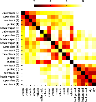
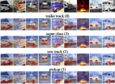
Figure 6: Left: Concept similarities (based on the Grassmann distance) between selected ImageNet vehicle concepts. Rows and columns are sorted correspondingly (“trailer truck (0)”). Rows are labeled according to class name and concept number whereas columns show manually tagged labels. High concept similarities correspond to small Grassmann distances. Note that background and object concepts are disentangled. Right: Transferring and comparing the “wheel” concept from different vehicle classes on random test samples from different classes (first row). The rows below show concept maps obtained from applying the four most similar “wheel” concepts from Figure 6.

Next, we perform a two-fold experiment. Firstly, akin to the previous analysis, we compare the four most similar concepts compared to the trailer truck (0)/’wheel’ concept. Secondly, we test concept transferability by applying all concepts onto random test samples originating from different classes. This is non-trivial and usually not possible with simple one-dimensional concept spaces. Results are shown in Figure 6. All four-wheel concepts are visually nearly indistinguishable. Additionally, all concepts transfer to samples from different classes. Again, this is fundamentally tied to the robust subspaces found by SSCCD. These findings further hint towards actual regions in feature space, which are activated if a certain pattern/concept is present in the input. In particular, these regions are found independent whether trained on single- or on superclass training samples. Similar results for the “window” and “street” concepts are presented in the supplementary material and further support our arguments. Overall, our experiment strengthens the notion of robustness, transferability and consistency associated with SSCCD.

4.5 Concept flipping

To provide a quantitative comparison to previous concept discovery methods, we invoke the Smallest Destroying Concepts (SDC) benchmark as proposed in [7] and [24]. To evaluate SDC, we subsequently remove concepts, i.e. the corresponding segments, in the order of their sample-wise relevance starting from high to low. We use images from ten ImageNet classes, which roughly align with CIFAR10 classes, and measure the (maximum) model accuracy on the selected subset of classes. We use a ResNet50 model and extract concepts from the penultimate ResNet block for ACE [7], the PCA/ICE-baseline described in Section 4.1 and SSCCD. ACE does not provide a measure of per-sample concept relevance. Therefore, we revert to the order of their TCAV scores after discarding concepts where statistical testing in comparison to random input samples fails to stay below $p=0.05$. We remove segments based on a classical imputation algorithm [35]. This results in more realistic imputed images. Thus, the model is evaluated on-manifold in contrast to imputing with gray patches as often done in the literature. For similar reasons, we avoid the Smallest Sufficient Concepts (SSC) benchmark, which would require high-quality imputation algorithms to avoid evaluating the model far from the data manifold. For SSCCD and the PCA/ICE-baseline, we compute concept relevance by employing PredDiffwith the same imputation method in input space. It is worth stressing again that SSCCD is indifferent to attribution methods. In particular, the concept ranking is not sensitive to this choice.

SSCCD	PCA	ACE	SDC experiment

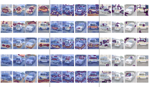
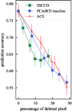
Figure 7: Left: Qualitative comparison between SSCCD, PCA/ICE-baseline and ACE based on random validation set samples from the ImageNet police van class. Right: Concept flipping (Smallest Destroying Concepts) benchmark comparing SSCCD and ACE[7]. Concepts are flipped once at a time in descending order of concept relevance/TCAV score, respectively. We measure the decline in model accuracy. Meaningful concept discovery and quantification methods are supposed to show a sharp decline in this figure. The importance of the attribution method is assessed by also flipping discovered concept segments in random order.

In the left panel of Figure 7, we qualitatively compare concepts identified by ACE, ICE/PCA and SSCCD. The ACE concepts are expressed only in a fraction of the images and, opposed to SCCDD, it is difficult to identify coherent, meaningful structures. This is in contrast to the much more coherent impression of the same ACE concepts visualized on training set samples, see supplementary material. Therefore, we suspect that generalization of concepts identified on training set samples to the test set is difficult for ACE. As observed in Section 4.1, the PCA concepts in Figure 7 are less coherent and localized than SSCCD concepts.

In the right panel of Figure 7, we show the results of the SDC experiment. In contrast to previous studies [7, 24], we report the model performance depending on the fraction of occluded pixels, which is essential for comparability since the segment size varies between different approaches. SSCCD shows the sharpest decline and is hence considered the superior approach for concept-based explanations. The slight increase in accuracy after flipping the last SSCCD concept is likely due to flipping i.e. removing slightly negatively attributed features from the background while parts of the relevant region are still visible (as previous concepts are localized). While SDC as a benchmark for concept explanations shows a favorable outcome for the proposed method, it entails several shortcomings: The quantitative results, albeit in most cases not the method ranking, may strongly depend on the imputation algorithm. Model scores for heavily occluded images are potentially unreliable due to off-manifold evaluation. Lastly, one needs to disentangle concept attribution and discovery. This ideally allows to change only a single component and therefore enable for more consistent comparisons.

5 Summary and Discussion

In this work, we provide a new definition of concepts as linear subspaces in feature space and present a constructive way of discovering them by means of sparse subspace clustering. Our experiments demonstrate a number of insights from SSCCD that are infeasible to obtain from standard pixel-wise attributions or existing concept-based interpretability methods. These range from a similarity measure for concept subspaces, over to concept maps that spatially resolve the concept expression for a specific sample, to the ability to quantify a concept’s relevance on a per-example basis via a user-specified local attribution method.

Appendix A One-dimensional SSCCD concepts (Section 4.1)

In Figure 8 to Figure 13, we revisit the discussion on the multidimensional nature of concepts. We use the “basketball”, “mobile home” and “electric locomotive” class as representatives for a class with a high intra-class variance and the “golden retriever”, “african grey” and “indian elphant” class as representatives for a class with small intra-class variance. As discussed in the main text, the PCA concepts come out more consistent in the latter case. We go beyond the discussion in the main text by also showing concept maps, where we reduce the subspaces identified via SSCCD to their first PCA component i.e. one-dimensional subspaces. This can be used to identify the dominant aspect underlying a specific concept subspace, it avoids the issues of double-counting closely related directions in feature space that would have appeared as separate concepts in the PCA approach. These results indicate that also one-dimensional concepts can entail a certain value but only if they are determined in an appropriate way. In this case, they are based on the already identified multidimensional SSCCD concepts, which could in this case be used directly instead.

SSCCD	SSCCD 1D	PCA

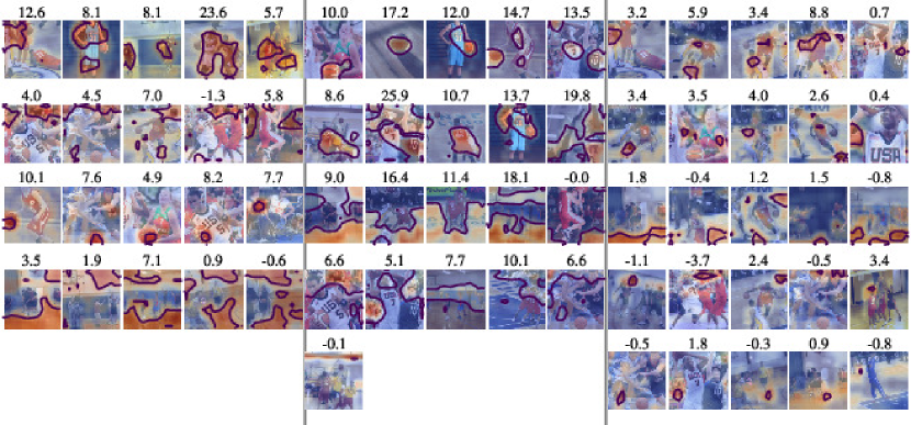
Figure 8: Concept maps for a VGG16 model (final convolutional layer) and the “basketball” class with high intra-class diversity. We compare multi-dimensional SSCCD concepts (left) to SSCCD concepts with a one-dimensional basis (middle) and one-dimensional concepts (right) obtained via direct application of PCA in feature space. In all three cases rows are ordered according to average concept relevance.

SSCCD	SSCCD 1D	PCA

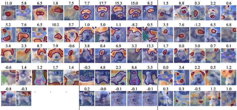
Figure 9: Concept maps for a VGG16 model (final convolutional layer) and the “golden retriever” with low intra-class diversity. We compare multi-dimensional SSCCD concepts (left) to SSCCD concepts with a one-dimensional basis (middle) and one-dimensional concepts (right) obtained via direct application of PCA in feature space. In all three cases rows are ordered according to average concept relevance.

SSCCD	SSCCD 1D	PCA

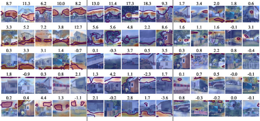
Figure 10: Concept maps for a VGG16 model (final convolutional layer) and the “mobile home” class with high intra-class diversity. We compare multi-dimensional SSCCD concepts (left) to SSCCD concepts with a one-dimensional basis (middle) and one-dimensional concepts (right) obtained via direct application of PCA in feature space. In all three cases rows are ordered according to average concept relevance.

SSCCD	SSCCD 1D	PCA

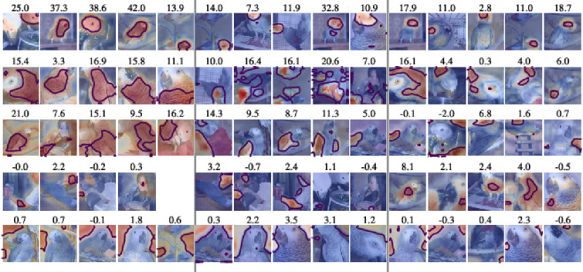
Figure 11: Concept maps for a VGG16 model (final convolutional layer) and the “african grey” class with low intra-class diversity. We compare multi-dimensional SSCCD concepts (left) to SSCCD concepts with a one-dimensional basis (middle) and one-dimensional concepts (right) obtained via direct application of PCA in feature space. In all three cases rows are ordered according to average concept relevance.

SSCCD	SSCCD 1D	PCA

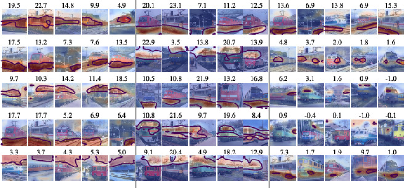
Figure 12: Concept maps for a VGG16 model (final convolutional layer) and the “electric locomotive” class with high intra-class diversity. We compare multi-dimensional SSCCD concepts (left) to SSCCD concepts with a one-dimensional basis (middle) and one-dimensional concepts (right) obtained via direct application of PCA in feature space. In all three cases rows are ordered according to average concept relevance.

SSCCD	SSCCD 1D	PCA

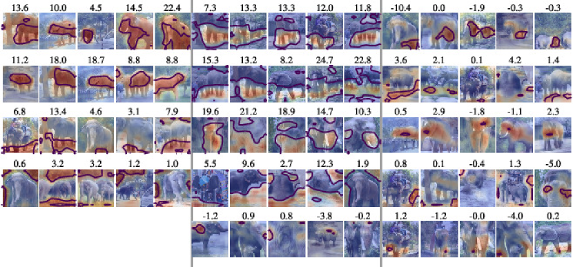
Figure 13: Concept maps for a VGG16 model (final convolutional layer) and the “indian elephant” class with low intra-class diversity. We compare multi-dimensional SSCCD concepts (left) to SSCCD concepts with a one-dimensional basis (middle) and one-dimensional concepts (right) obtained via direct application of PCA in feature space. In all three cases rows are ordered according to average concept relevance.

Appendix B More ImageNet classes for VGG16/ResNet50 (Section 4.2)

In Figure 14 to Figure 17, we present further concept maps for four randomly selected ImageNet classes comparing VGG16 (last convolutional layer) to ResNet50 (penultimate ResNet block) concepts. All four figures are structured identically: Each row corresponds to a particular concept identified by SSCCD. The rows are sorted according to mean concept relevance (for every architecture separately) assessed via Integrated Gradients in the input space. The eight leftmost pictures show VGG16 concept maps, the eight rightmost pictures correspond to ResNet50. Among these groups of eight pictures the four leftmost pictures show the pictures that were activated most by the concept (in terms of sample-concept proximity), which gives in most cases the best overall impression what the concept signifies. The remaining four pictures show concept maps for four randomly selected pictures from the corresponding test dataset. These give an impression how consistently a concept is expressed in the dataset in terms of a selection with no selection bias. On top of each picture we also indicate the per-example concept relevance (again assessed via Integrated Gradients in input space) for samples where the sample-concept proximity reached a value below the concept-specific threshold angle.

In most cases, one finds consistent human-identifiable concepts (with the exception of a few concepts that are not activated in the test set at all and a few elongated structures in the case of ResNet50 both of which we mark as “empty”) which we also indicate in the figure captions. These reveal interesting differences between the model architectures that are supposed to be investigated in future studies.

VGG16		ResNet50
highly activated	randomly selected	highly activated	randomly selected

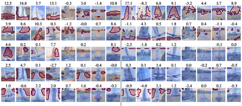
Figure 14: Concept maps for the ImageNet class “trimaran”. For VGG16 the concepts can be roughly identified with hull, mast/sail, rigging, water, sky and for ResNet50 with rigging, water, empty/sky, empty/sky, sky.

VGG16		ResNet50
highly activated	randomly selected	highly activated	randomly selected

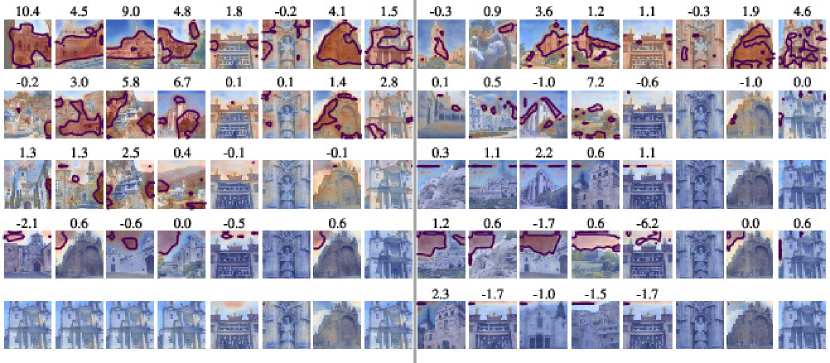
Figure 15: Concept maps for the ImageNet class “monastery”. For VGG16 the the concepts can be roughly identified with fancy facade, simple facade, trees, sky, empty and for ResNet50 with facade, roof, empty/sky, sky, empty/sky.

VGG16		ResNet50
highly activated	randomly selected	highly activated	randomly selected

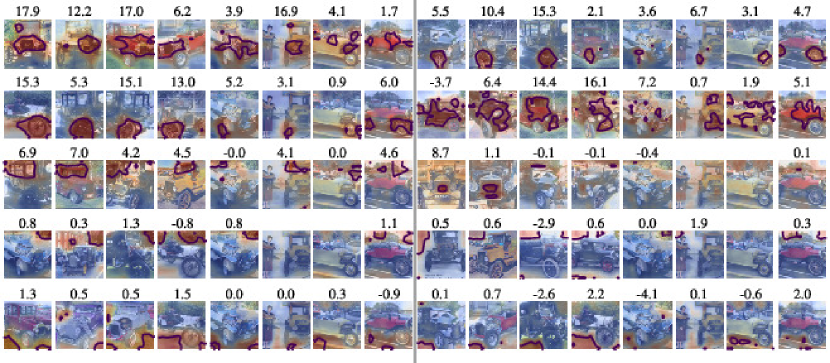
Figure 16: Concept maps for the ImageNet class “Model T”. For VGG16 the concepts can be roughly identified as lights, wheels, windows, trees, street and for ResNet50 as wheels, hood, radiator grill, sky, ground.

VGG16		ResNet50
highly activated	randomly selected	highly activated	randomly selected

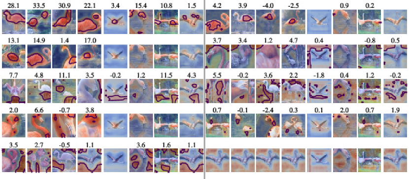
Figure 17: Concept maps for the ImageNet class “flamingo”. For VGG16 the concepts can be roughly identified as body, wing feathers, legs, head/neck, water and for ResNet50 as feather wings, background, water, legs/neck, empty.

Appendix C Layer-dependence (Section 4.2)

We compare concepts of the penultimate ResNet50 block with concepts of the final block in Figure 18 to assess the dependency of SSCCD concepts on the model layer. Concepts from the final block are broader than concepts at the penultimate block in the sense that they cover multiple components of the object, e.g. the first concept relates to the entire upper part of the police van including part of the car body, windows and buildings in the background. In contrast, concepts at the penultimate block can be identified with specific parts of the police van, like car body, emergency lights or tires. While this finding might be partially explained by the resizing factor between concept maps in feature and input space which is two times larger for the final block, it aligns with the common observation that the abstraction level increases for higher convolutional layers.

ResNet50 block
penultimate                        final

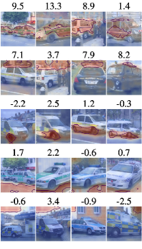
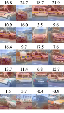
Figure 18: Concept maps for the ImageNet “police van” class at the penultimate ResNet50 block (left) and at the final block of a ResNet50 model.

Appendix D Varying the number of concepts (Section 4.2)

In Figure 19, we demonstrate the impact of varying the number of concepts (for fixed, precomputed self-representation) at the example of the ImageNet class “police van”. It shows how new concepts emerge and how existing concepts subdivide to form more finegrained concepts. For more than 5 concepts, also VGG16 also shows the “emergency lights” concept that was only observed for ResNet50 at a fixed number of 5 clusters.

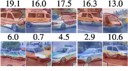
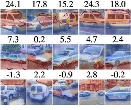
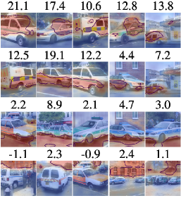
$n_{\text{concepts}}=2$	$n_{\text{concepts}}=3$	$n_{\text{concepts}}=4$
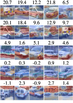
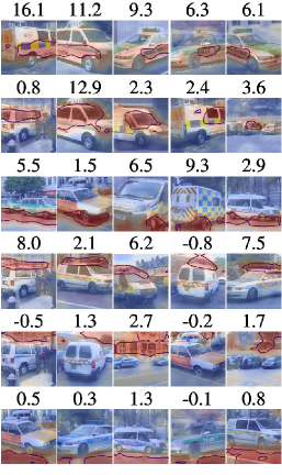
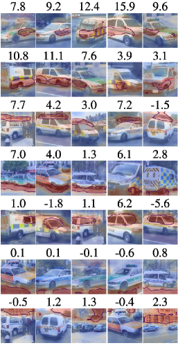
$n_{\text{concepts}}=5$	$n_{\text{concepts}}=6$	$n_{\text{concepts}}=7$

Figure 19: Concept maps for police van class and a VGG16 model (final convolutional layer) varying the number of concepts from 2 to 7, where we show the most activated examples (in the sense of sample-concept proximity). Determining the number of concepts via the largest gap in the spectrum yields only yields a value of 2 in this case.

Appendix E More CelebA (anti-)class concepts (Section 4.3)

To support the findings in Section 4.3, we show concepts for more attributes of the CelebA dataset in Figure 20 to Figure 22. Additionally, we show concepts for the respective inverse attribute. These support the findings discussed in the main text, which we reiterate here for completeness: The identified concepts are highly specific both in terms of localization (c.f. chin for “male” vs. neck/hair for “female”) and in terms of underlying features. The latter can be inferred from the fact that similarly localized concepts (e.g. nose for “male”/“female”, hair for “young/old”) are found for class and anti-class but evaluating a particular concept only weakly activates the corresponding region with the anti-concept.

male concepts			female concepts
male samples	female samples		female samples	male samples

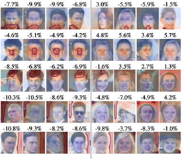
Figure 20: SSCCD concepts on CelebA for a ResNet50 model for samples with the “male” (left) and “female” (right) attribute. Concepts are ordered according to average concept relevance showing samples with smallest sample-concept proximity. We apply the same male concept on a random selection of female samples and vice-versa. Subtitles indicate the sample-concept proximity of samples relative to the normalized sample-concept proximity $\delta^{iA}/\delta^{A}$, i.e. samples with values $<1$ are (highly) activated. The “male” concepts can be roughly identified as chin, nose, hair(line), background, background and neck/hair, nose, background, hair, background for “female”.

young concepts			old concepts
young samples	old samples		old samples	young samples

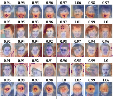
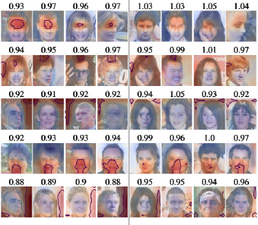
Figure 21: SSCCD concepts on CelebA for a ResNet50 model for samples with the “young” (left) and “old” (right) attributes. Concepts are ordered according to average concept relevance showing samples with smallest sample-concept proximity. We apply the same young concept on a random selection of old samples and vice-versa. Subtitles indicate the sample-concept proximity of samples relative to the normalized sample-concept proximity $\delta^{iA}/\delta^{A}$, i.e. samples with values $<1$ are (highly) activated. The “young” concepts can be roughly identified with mouth, hair, background, background, between eyes and forehead, hair, background, mouth/nose, background for “old”.

smiling concepts			not smiling concepts
smiling samples	not smiling samples		not smiling samples	smiling samples

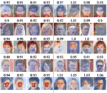
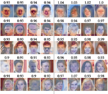
Figure 22: SSCCD concepts on CelebA for a ResNet50 model for samples with the “smiling” (left) and “not smiling” (right) attributes. Concepts are ordered according to average concept relevance showing samples with smallest sample-concept proximity. We apply the same smiling concept on a random selection of not smiling samples and vice-versa. Subtitles indicate the normalized sample-concept proximity $\delta^{iA}/\delta^{A}$, i.e. samples with values $<1$ are (highly) activated. The “smiling” concepts can be roughly identified with chin/mouth, background, hair(line), background, nose and nose, background, hair, background, background in the case of “not smiling”.

Appendix F More concepts transfer experiments (Section 4.4)

To further support the findings in Figure 6, we additionally show the transferability for two more concepts in Figure 23. Again, we find that all similar concepts are visually closely related and transfer in a sensible manner on all test samples.

street concept	window concept

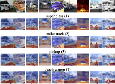
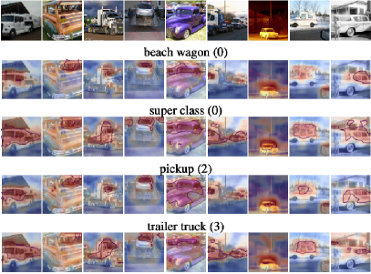
Figure 23: Transferring and comparing the street/window concept from different vehicles classes on random test samples. Four most similar concepts according Figure 6.

Appendix G ACE concepts visualized on training set samples (Section 4.5)

Due to the difficulty of identifying coherent, meaningful structures in the ACE concepts visualized on validation set samples in Figure 7 we show the same concepts on training set samples in Figure 24. Here, we can roughly identify background structures, police van body, windows, street and greenery. We suspect that generalization of concepts identified on training set samples to the test set is difficult for ACE.

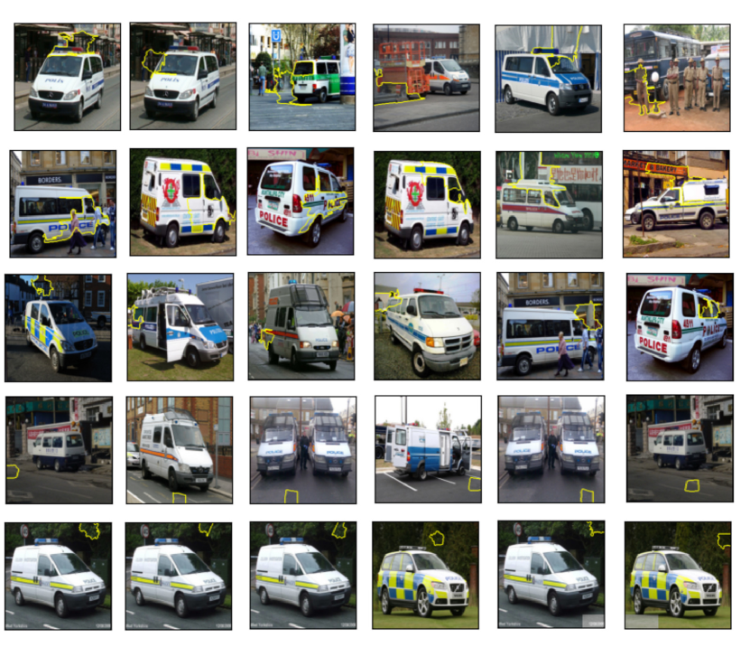
Figure 24: ACE concepts as shown in Figure 7 visualized on training set samples. Each row corresponds to one concept. Like in Figure 7, we show the five most important concepts ordered by their TCAV scores from top row to bottom row. We can roughly identify background structures, police van body, windows, street and greenery.

Appendix H Rank-consistency of attribution methods for concept relevance

The concept importance scores presented in this work are based on Integrated Gradients attributions. We obtain per-sample concept relevances by summing over these attributions in the thresholded regions of the concept maps in input space. For class-wise concept relevance scores, we average over all per-sample scores in the class. Here, we assess the effect of this relevance quantification method. Firstly, we replaced Integrated Gradients with PredDiff and secondly, measure attributions in feature space directly (for both methods). For Integrated Gradients, we use 200 steps and the dataset mean as a baseline. For PredDiff, we occlude each concept region using a train set imputer and 100 imputations. In Table 1, we show the median Spearman rank correlation between class-wise concept importance scores across 42 random classes from the ImageNet dataset. The concepts stem from the last convolutional layer of VGG16. While there are differences in the numerical values, the high median correlation coefficients in Table 1 demonstrates that the concept ranking is consistent across all methods.

	IG FS	IG IS	PredDiff  FS	PredDiff  IS
IG  FS	1.0	1.0	0.9	0.9
IG  IS	1.0	1.0	0.9	0.9
PredDiff FS	0.9	0.9	1.0	0.9
PredDiff  IS	0.9	0.9	0.9	1.0

Table 1: Median Spearman rank correlation coefficient between concept importance scores from Integrated Gradients (IG) and PredDiff in input space (IS) and feature space (FS) for concepts across 42 random classes from the ImageNetdataset and VGG16 (last convolutional layer).

Appendix I Source code and hyperparameter choices

As part of this supplementary material, we provide source code to train custom models on CelebA data, to compute self-representations for a given dataset and pretrained model, to identify clusters via spectral clusters and to determine the corresponding bases for concept subspaces. Here, we provide basic usage information.

I.1 Training a custom model on CelebA

Listing 1: CelebA training call

⬇

#!/bin/bash

python imagenet_e2e.py –data path_to_celeba_data –dataset celeba

I.2 Computing self-representation, clustering and concept subspaces

In all our experiments, we fix the noise-controlling hyperparameter to $\gamma=10$. We choose $\tau=1.0$ for the hyperparameter corresponding to the elastic net penalty term. Lastly, we use two batches of 64 samples each and subsample features at a rate of $0.8$. Only for the final ResNet50 block, we use eight batches to account for the spatially smaller feature maps. Below, we provide an example for computing the self-representation, spectral clustering and subspace bases for the last convolutional layer (penultimate block) of VGG16 (ResNet50) and the ImageNet police van class.

Listing 2: SSCCD usage

⬇

import concept_ssc

# SSCCD for the imagenet police van class

# and the last convolutional layer (penultimate block) of VGG16 (ResNet50)

# (pretrained model from torchvision)

model_choice = ’vgg16’ # ’resnet50’

featurelayer_choice = 30 # 7

cssc = concept_ssc.ConceptSSC(ssc_method=’elasticnet’, n_concepts=5, gamma=10, tau=1.0, n_batches=2, batch_size=64, feature_subsample_ratio=0.8, featurelayer=featurelayer_choice, model_arch=model_choice, dataset=’imagenet’, datapath=’./’, selected_classes=["police van",])

# compute self-representation and spectral clustering

cssc.fit(out_dir=’./’)

# determine bases for concept subspaces

bases = cssc.conceptspace_bases()

References

- Kiefer and Pulvermüller [2012] Markus Kiefer and Friedemann Pulvermüller. Conceptual representations in mind and brain: Theoretical developments, current evidence and future directions. Cortex, 48(7):805–825, July 2012. doi: 10.1016/j.cortex.2011.04.006. URL https://doi.org/10.1016/j.cortex.2011.04.006.
- Covert et al. [2021] Ian Covert, Scott Lundberg, and Su-In Lee. Explaining by removing: A unified framework for model explanation. Journal of Machine Learning Research, 22(209):1–90, 2021.
- Lundberg and Lee [2017] Scott M Lundberg and Su-In Lee. A unified approach to interpreting model predictions. In Advances in neural information processing systems, pages 4765–4774, 2017.
- Montavon et al. [2018] Grégoire Montavon, Wojciech Samek, and Klaus-Robert Müller. Methods for interpreting and understanding deep neural networks. Digital Signal Processing, 73:1–15, 2018.
- Samek et al. [2021] Wojciech Samek, Grégoire Montavon, Sebastian Lapuschkin, Christopher J. Anders, and Klaus-Robert Müller. Explaining deep neural networks and beyond: A review of methods and applications. Proceedings of the IEEE, 109(3):247–278, 2021. doi: 10.1109/JPROC.2021.3060483.
- Kim et al. [2018] Been Kim, Martin Wattenberg, Justin Gilmer, Carrie Cai, James Wexler, Fernanda Viegas, et al. Interpretability beyond feature attribution: Quantitative testing with concept activation vectors (tcav). In International conference on machine learning, pages 2668–2677. PMLR, 2018.
- Ghorbani et al. [2019] Amirata Ghorbani, James Wexler, James Y Zou, and Been Kim. Towards automatic concept-based explanations. Advances in Neural Information Processing Systems, 32:9277–9286, 2019.
- Yeh et al. [2020] Chih-Kuan Yeh, Been Kim, Sercan Arik, Chun-Liang Li, Tomas Pfister, and Pradeep Ravikumar. On completeness-aware concept-based explanations in deep neural networks. In H. Larochelle, M. Ranzato, R. Hadsell, M. F. Balcan, and H. Lin, editors, Advances in Neural Information Processing Systems, volume 33, pages 20554–20565. Curran Associates, Inc., 2020. URL https://proceedings.neurips.cc/paper/2020/file/ecb287ff763c169694f682af52c1f309-Paper.pdf.
- Elhamifar and Vidal [2013] Ehsan Elhamifar and René Vidal. Sparse subspace clustering: Algorithm, theory, and applications. IEEE transactions on pattern analysis and machine intelligence, 35(11):2765–2781, 2013.
- Selvaraju et al. [2020] Ramprasaath R Selvaraju, Michael Cogswell, Abhishek Das, Ramakrishna Vedantam, Devi Parikh, and Dhruv Batra. Grad-cam: Visual explanations from deep networks via gradient-based localization. International Journal of Computer Vision, 128(2):336–359, 2020.
- Soltanolkotabi and Candes [2012] Mahdi Soltanolkotabi and Emmanuel J Candes. A geometric analysis of subspace clustering with outliers. The Annals of Statistics, 40(4):2195–2238, 2012.
- You et al. [2016a] Chong You, Daniel Robinson, and René Vidal. Scalable sparse subspace clustering by orthogonal matching pursuit. In Proceedings of the IEEE conference on computer vision and pattern recognition, pages 3918–3927, 2016a.
- You et al. [2016b] Chong You, Chun-Guang Li, Daniel P Robinson, and René Vidal. Oracle based active set algorithm for scalable elastic net subspace clustering. In Proceedings of the IEEE conference on computer vision and pattern recognition, pages 3928–3937, 2016b.
- Von Luxburg [2007] Ulrike Von Luxburg. A tutorial on spectral clustering. Statistics and computing, 17(4):395–416, 2007.
- Fukunaga and Olsen [1971] Keinosuke Fukunaga and David R Olsen. An algorithm for finding intrinsic dimensionality of data. IEEE Transactions on Computers, 100(2):176–183, 1971.
- Bac et al. [2021] Jonathan Bac, Evgeny M. Mirkes, Alexander N. Gorban, Ivan Tyukin, and Andrei Zinovyev. Scikit-dimension: a python package for intrinsic dimension estimation. arXiv preprint 2109.02596, 2021.
- Caron et al. [2021] Mathilde Caron, Hugo Touvron, Ishan Misra, Hervé Jégou, Julien Mairal, Piotr Bojanowski, and Armand Joulin. Emerging properties in self-supervised vision transformers. In International Conference on Computer Vision, 2021.
- Jordan [1875] Camille Jordan. Essai sur la géométrie à dimensions. Bulletin de la Société Mathématique de France, 3:103–174, 1875. doi: 10.24033/bsmf.90.
- Blücher et al. [2021] Stefan Blücher, Johanna Vielhaben, and Nils Strodthoff. Preddiff: Explanations and interactions from conditional expectations. arXiv preprint 2102.13519, 2021.
- Robnik-Sikonja and Kononenko [2008] M. Robnik-Sikonja and I. Kononenko. Explaining classifications for individual instances. IEEE Transactions on Knowledge and Data Engineering, 20(5):589–600, May 2008. doi: 10.1109/tkde.2007.190734.
- Sundararajan et al. [2017] Mukund Sundararajan, Ankur Taly, and Qiqi Yan. Axiomatic attribution for deep networks. In International Conference on Machine Learning, volume 70, pages 3319–3328. JMLR, 2017.
- Li et al. [2021] Jiahui Li, Kun Kuang, Lin Li, Long Chen, Songyang Zhang, Jian Shao, and Jun Xiao. Instance-wise or class-wise? a tale of neighbor shapley for concept-based explanation. In Proceedings of the 29th ACM International Conference on Multimedia, MM ’21, page 3664–3672, New York, NY, USA, 2021. Association for Computing Machinery. ISBN 9781450386517. doi: 10.1145/3474085.3475337. URL https://doi.org/10.1145/3474085.3475337.
- Hamm [2008] Jihun Hamm. Subspace-based learning with Grassmann kernels. PhD thesis, University of Pennsylvania, 2008.
- Wu et al. [2020] Weibin Wu, Yuxin Su, Xixian Chen, Shenglin Zhao, Irwin King, Michael R. Lyu, and Yu-Wing Tai. Towards global explanations of convolutional neural networks with concept attribution. In Proceedings of the IEEE/CVF Conference on Computer Vision and Pattern Recognition (CVPR), June 2020.
- Zhang et al. [2021] Ruihan Zhang, Prashan Madumal, Tim Miller, Krista A Ehinger, and Benjamin IP Rubinstein. Invertible concept-based explanations for cnn models with non-negative concept activation vectors. In Proceedings of the AAAI Conference on Artificial Intelligence, volume 35, pages 11682–11690, 2021.
- Kumar et al. [2021] Ashish Kumar, Karan Sehgal, Prerna Garg, Vidhya Kamakshi, and Narayanan Chatapuramkrishnan. Mace: Model agnostic concept extractor for explaining image classification networks. IEEE Transactions on Artificial Intelligence, pages 1–1, 2021. doi: 10.1109/TAI.2021.3111138.
- Kamakshi et al. [2021] Vidhya Kamakshi, Uday Gupta, and Narayanan C Krishnan. Pace: Posthoc architecture-agnostic concept extractor for explaining cnns. In 2021 International Joint Conference on Neural Networks (IJCNN), pages 1–8, 2021. doi: 10.1109/IJCNN52387.2021.9534369.
- Bau et al. [2017] David Bau, Bolei Zhou, Aditya Khosla, Aude Oliva, and Antonio Torralba. Network dissection: Quantifying interpretability of deep visual representations. In Proceedings of the IEEE conference on computer vision and pattern recognition, pages 6541–6549, 2017.
- Fong and Vedaldi [2018] Ruth Fong and Andrea Vedaldi. Net2vec: Quantifying and explaining how concepts are encoded by filters in deep neural networks. In Proceedings of the IEEE conference on computer vision and pattern recognition, pages 8730–8738, 2018.
- Zhou et al. [2018] Bolei Zhou, Yiyou Sun, David Bau, and Antonio Torralba. Interpretable basis decomposition for visual explanation. In Proceedings of the European Conference on Computer Vision (ECCV), September 2018.
- Deng et al. [2009] Jia Deng, Wei Dong, Richard Socher, Li-Jia Li, Kai Li, and Li Fei-Fei. Imagenet: A large-scale hierarchical image database. In 2009 IEEE conference on computer vision and pattern recognition, pages 248–255. Ieee, 2009.
- Liu et al. [2015] Ziwei Liu, Ping Luo, Xiaogang Wang, and Xiaoou Tang. Deep learning face attributes in the wild. In Proceedings of International Conference on Computer Vision (ICCV), December 2015.
- Simonyan and Zisserman [2014] Karen Simonyan and Andrew Zisserman. Very deep convolutional networks for large-scale image recognition. In International Conference on Learning Representations, 2014.
- He et al. [2016] Kaiming He, Xiangyu Zhang, Shaoqing Ren, and Jian Sun. Deep residual learning for image recognition. In Proceedings of the IEEE conference on computer vision and pattern recognition, pages 770–778, 2016.
- Bertalmio et al. [2001] Marcelo Bertalmio, Andrea L Bertozzi, and Guillermo Sapiro. Navier-stokes, fluid dynamics, and image and video inpainting. In Proceedings of the 2001 IEEE Computer Society Conference on Computer Vision and Pattern Recognition. CVPR 2001, volume 1, pages I–I. IEEE, 2001.