Embedding Earth: Self-supervised contrastive pre-training for dense land cover classification

Abstract

In training machine learning models for land cover semantic segmentation there is a stark contrast between the availability of satellite imagery to be used as inputs and ground truth data to enable supervised learning. While thousands of new satellite images become freely available on a daily basis, getting ground truth data is still very challenging, time consuming and costly. In this paper we present Embedding Earth a self-supervised contrastive pre-training method for leveraging the large availability of satellite imagery to improve performance on downstream dense land cover classification tasks. Performing an extensive experimental evaluation spanning four countries and two continents we use models pre-trained with our proposed method as initialization points for supervised land cover semantic segmentation and observe significant improvements up to $25\%$ absolute mIoU. In every case tested we outperform random initialization, especially so when ground truth data are scarse. Through a series of ablation studies we explore the qualities of the proposed approach and find that learnt features can generalize between disparate regions opening up the possibility of using the proposed pre-training scheme as a replacement to random initialization for Earth observation tasks. Code will be uploaded soon at https://github.com/michaeltrs/DeepSatModels.

I Introduction

In recent years an increasing number of organizations have placed emphasis on the use of Earth observation (EO) data and machine learning technologies as a means to partially automate or enchance their capacity in setting, monitoring and reporting the progress made on their associated goals and targets. Such technologies could be applied for projects ranging from global scale to benefiting targeted communities in need [1]. The United Nations (UN) aim at using remote sensing data for monitoring sustainable development goals [2]. In the European Union (EU) part of the Common Agricultural Policy (CAP) objectives is the use of remote sensing tools for the automation and monitoring of CAP allocations and sustainability targets . In Africa the use of satellite imagery for crop yield prediction and early detection of pests and plant diseases could lead to almost real time monitoring of food supplies and the prevention of potential shortages [3].

At the same time driven by potential benefits an increasing number of EO satellites are getting launched collecting data for Earth systems and monitoring the variability in natural and built environments. For Sentinel-1/2 satellite missions alone the total amount of data available to download has already reached the Petabyte scale. This plethora of input data is in stark contrast to the difficulty of obtaining ground truth annotations, especially at the scale required to make the most out of supervised deep learning alghorithms which have revolutionized computer vision [4, 5, 6]. Compiling ground truth datasets for EO tasks involves the collection of data either through the deployment of field missions or the development of platforms for crowd sourcing data [7]. Both solutions are time consuming and costly especially so for remote and difficult to access regions.

This imbalance necessitates the development of techniques for learning without annotations that can leverage the large amounts of readily available available EO data. In this paper, we propose such a method for self-supervised learning of dense representations. Our key contributions are the following:

1. we design a system for end-to-end self-supervised visual pre-training at the pixel level. Finetuning the pre-trained models on land cover semantic segmentation we observe significant improvements up to $25\%$ absolute mIoU compared to our baselines. Benefits are particularly pronounced for datasets containing relatively few annotations.

2. through a series of ablation studies we explore the method hyperparameter space and derive conclusions about how the size and qualitative characteristics of the pre-training set affect downstream segmentation performance. We find that increasing the size of the pre-training set, either by extending the Period of Interest (POI) or the Area of Interest (AOI), generally improves downstream segmentation performance.

3. we find no performance deterioration when initializing from a model pre-trained in a different region than the AOI of the downstream segmentation task, e.g. pre-training a model on a different country compared to pre-training using at the same AOI as the annotated dataset. This observation opens the possibility for the general use of such pre-trained models as initialization points for land cover segmentation tasks. We make the pre-trained models used in this study publicly available together with code for replicating the experiments presented here.

II Related work

II-A Beyond random initialization of model parameters

When training DNNs an unfavourable initialization of model parameters can lead to several problems such as parameter saturation and very slow convergence to a good solution [8]. Several works have proposed techniques for stabilizing the training dynamics making it possible to train deeper architectures that lead to improved DNN performance overall [8, 9, 10, 11]. Beyond these insights regarding parameter initialization it has been found that rather than randomly initializing network parameters for every new task, using the weights of a model previously trained on a different domain can in many cases improve performance. Transfer Learning revolves around this idea: how to transfer knowledge which has been learnt into one source domain to another downstream target domain. A common practice for training DNNs for vision related tasks has been to use models trained on large scale image classification datasets, e.g. ImageNet [12] as an initialization point for downstream tasks [13]. For this setting to work knowledge learnt during pre-training needs to be general enough to find some application in the target domain. In that spirit it is convenient if there is some overlap between the semantic objects found in the pre-training and target domain datasets. Another approach following similar principles is to use un/self-supervised training prior to fine-tuning a network into the target domain. This approach has also been shown to improve performance [14] and has two distinct advantages compared to supervised transfer learning. First, unlabelled data are inexpensive to obtain making it easier to compile large scale datasets which contain significant variation and can be used to train models that generalize well to unseen data.Secondly, it makes it possible to compile a dataset and derive a pre-training methodology that is specifically tailored to the target domain and task. For dense classification tasks with remote sensing imagery our proposed method follows the latter approach of self-supervised pre-training. The main reason for this choice is the difficulty of obtaining annotations at high resolution over very large AOI and the inability of land cover classification models to generalize from one region to another as has been empirically shown in previous studies [15, 16].

II-B Metric learning

The main goal of metric learning is to express the similarity between different inputs by use of a distance metric over their encoded representations. For training DNNs the most commonly encountered framework for applying metric learning is to use Siamese Networks trained with a Contrastive loss function. Siamese Networks employ two copies of the same network used to process two inputs of known semantic similarity and obtain their respective encodings. Popular applications involve signature [17] and face [18] verification and one-shot image recognition [19]. A contrastive loss function is designed for reducing the distance between encodings of inputs characterized by similar semantics (positive pairs) and increasing the distance between pairs with different semantics (negative pairs). Originally introduced for face verification [18] there has recently been a resurgence of Contrastive learning methods in computer vision as a means for learning a useful embedding space and to enchance the discriminatory capacity of DNNs on downstream tasks. The method can be applied in either a fully supervised manner [20, 21, 22, 23, 24] or, by choice of a suitable pretext task, as a self-supervised learning task [25, 26, 27].

II-C Self-supervised learning for vision tasks

Before computer vision self-supervised learning approaches have driven a revolution in natural language processing (NLP). Models pre-trained on a large corpus of text significantly outperform their counterparts trained only using annotated data [28, 29, 30]. These methods typically employ autoencoders [31, 32, 33, 34] and in particular the masked autoencoder framework [35] in which part of the input is hidden and the learning task is to predict that in the output. For successfully doing so the model is expected to learn some underlying structure of the data and thus learn about the data space without requiring annotations. Several works in computer vision have used the same framework. Applying the BERT criterion [28] on natural images [36] hide and subsequently predict a fixed ratio of pixels in an autoregressive manner. Contrastive Predictive Coding (CPC) [26, 37] uses autoregressive modelling to predict the future in latent rather than input space. While this framework naturally suits problems involving sequential data a variety of problems can be formulated using this framework, e.g. for image classification an image can be seen as a series of patches extracted from a predefined grid.
A recently popularized framework for self-supervised learning in vision involves using instance discrimination [25] as a pretext task. Instance discrimination assumes that each sample in a training set belongs to a class of each own and the training task involves learning to discriminate each sample from all other samples. In a contrastive learning setting two different views of the same sample, obtained by data augmentation, should be mapped nearby in embedding space while all other inputs should be contrasted. We note how this framework does not require any annotations, the identities of the training samples alone are used to define a set of classes. In that spirit [25, 27, 38, 39, 40] use the instance discrimination task and variants of Noise Contrastive Estimation (NCE) loss [41]. They manage to learn high quality embedding spaces judged by the capacity of a linear classifier to separate produced embeddings into classes when trained on annotated data. These methods have contributed to closing the gap in the discriminative power between models trained in a fully supervised and self-supervised manner. It is generally agreed that comparing with a large number of negative pairs is required for a successful implementation. In [27, 38] this is achieved by use of a very large batch size. However, this imposes a requirement for large accelerator memory. To decouple the number of negative samples from the mini-batch size, allowing it to be large, [25] keep encodings for every sample in the training set in a memory bank which is updated when the same sample is encountered during each epoch. In the same spirit [39, 40] maintain a dynamic dictionary of encodings as a fixed size data queue. Our method uses the latter approach which is found to improve performance without the need of large batch sizes. Also, strong data augmentation and the addition of a separate 2-layer predictor network for obtaining final embeddings were both shown to improve performance in [27, 40]. In our proposed approach which is designed for use with satellite imagery data augmentation is driven by the characteristics of input domain. Additionally in preliminary experiments the use of a predictor network was not found to improve performance and is avoided in favour of simplicity.

All the above works were developed to learn global image representations suitable for image classification. More recently self-supervised instance discrimination was extended to a dense context in [42, 43]. Both works employ data queues and input augmentation to create two different views of a sample image. Positive pairs are obtained by sampling from a set of pixels in correspondence between the two views. While [42] keep track of augmentation parameters to derive pixel correspondences [43] opt to learn correspondences as a separate process during training. Additionally, [43] add a loss component on global features which they show to stabilize the learning process. Our work is more similar to [42] in that we only use local features and calculate explicit pixel correspondences. In contrast to both works we formulate our loss function to include pixels from the same sample into the set of negative pairs and extend the data augmentation module for use with image time-series.

II-D Land cover semantic segmentation using satellite imagery

Land cover semantic segmentation aims at classifying each location found in a satellite image, or a set of images, as one out of a predefined number of land cover types. The same techniques for training DNNs that have lead to significant advances in computer vision community have been consistently shown to outperform previous remote sensing based approaches either using single images [44, 45] or image time series of [46, 47, 48, 49]. However, the domain of satellite images is fundamentally different from that of natural images requiring special treatment for successful model training. For example while it is possible to compile large scale datasets of natural images from a variety of image sensors this is not possible with remote sensing data as satellite sensors are expensive to set in orbit and exhibit more variation between one another than RGB sensors do, e.g. in terms of resolution and image bands. As such most trained models tend to be sensor dependent. Moreover, regional variations in atmospheric conditions, land geometry and land cover types hinder the generalization capability of models trained with full supervision [15, 16] and obtaining large scale ground truth annotations at a scale that would make generalization possible has not been achieved thus far.
Tackling semantic segmentation of crop types from time series of satellite images [47] exploit the spatial temporal nature of the inputs and propose the use of CRNN framework [50] in which fully connected RNN layers are replaced by 2D convolutional layers. Improving their results [48] first process each image individually by a 2D CNN before applying a CRNN backend and also test a fully convolutional 3D-UNET [51]. Both models achieve similar performance. Exploring the use of pre-training methods [24] use a fully supervised contrastive criterion to model the relationship between each pixel and its local spatial context. Their work shows improvements over the aforementioned studies [47, 48] while exhibiting significant performance gains along parcel boundaries. Using [52] use the BDL framework [53] for semantic segmentation adversarial domain adaptation to improve the performance between static RGB images obtained from different satellites. In the self-supervised space [54] use the BERT criterion on time series of satellite images improving the performance of randomly initialized baselines. Their approach only uses individual pixels and thus does not perform joint spatio-temporal modelling which is a goal of this study. For static images [55] use semantic inpainting [56] for overhead scene parsing, road network extraction, and land cover estimation.

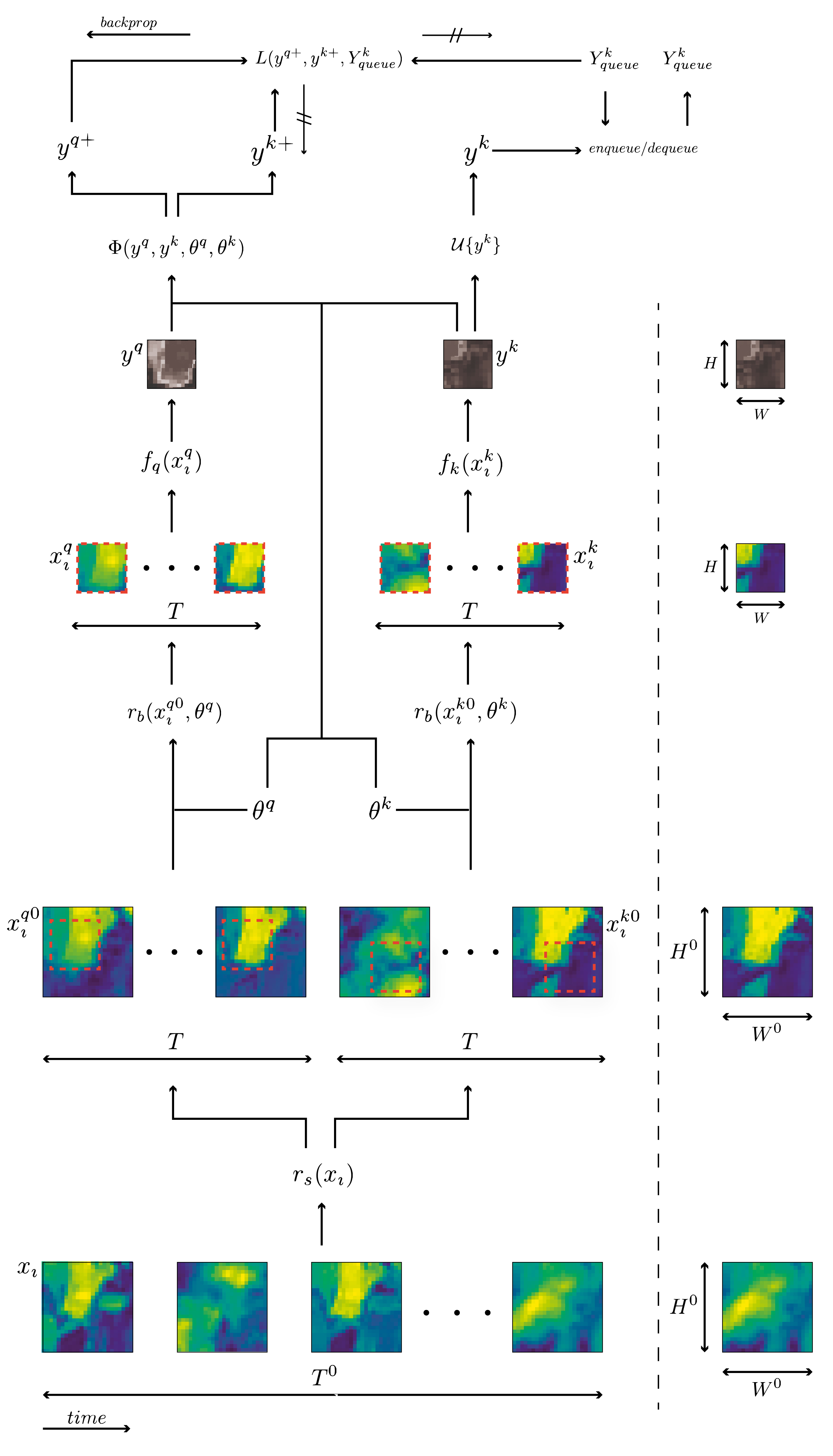
Figure 1: Overview of the proposed pre-training framework. Bottom to top: An input time series is processed by the sample ($r_{s}$) and batch ($r_{b}$) level augmentation modules to produce the inputs for the queries ($f_{q}$) and keys ($f_{k}$) encoders. The correspondence module $\Phi$ retrieves pixels in correspondence $y^{q+}$ and $y^{k+}$ from extracted embeddings $y^{q}$ and $y^{k}$ which are used to form positive and in-sample negative pairs. These features, together with the data queue $Y^{k}_{queue}$ are used to derive the current loss. Backpropagation is applied only for the queries encoder. After parameter update the earliest encodings are dequeued and $N_{queue}$ randomly sampled embeddings $y^{k}$ are enqueued.

III Proposed approach

Our proposed method can be categorized as a dense instance discrimination pretext task. In particular we make the assumption that pixels corresponding to the same location over the span of a POI correspond to the same land cover type. Thus, we force extracted features corresponding to the same location under different views in space and time to be similar. At the same time we assume that no two locations have the exact same characteristics, thus, we optimize our feature extractor such that features extracted at different locations are dissimilar irrespective of view. Overall our training pipeline includes the following components:

1. a stochastic data augmentation module $r(\cdot)$ is used to extract two different views for every sample in a mini-batch of image time series.

2. queries and keys encoder functions $f_{q}(\cdot),f_{k}(\cdot)$ extract pixel level encodings for each respective view.

3. a dense correspondence module $\Phi(\cdot)$ is used to find pairs of pixels corresponding to the same location from the two views (positive pairs). All other pairs are considered to be negative pairs,

4. a data queue $K$ in which key encodings from the current mini-batch are enqueued while these from the oldest one are dequeued.

5. a contrastive loss function $L(\cdot)$ is used to encourage extracted encodings from positive pairs to be close in embedding space and far for all negative pairs.

All model components are presented schematically in Fig.1 and in Python pseudocode in Listing 2. In the following sections we describe each component individually.

III-A Extracting different views

To ensure an efficient implementation our data augmentation module is decomposed into two separate modules $r=r_{b}\circ r_{s}$ at the sample and batch levels. Separately for each sample $x_{i}\in\mathbb{R}^{T_{i}\times H\times W\times C}$ in a mini-batch $X=\{x_{i}\},i\in\{1,...,N\}$ the sample level module extracts two views $x_{i}^{qs},x_{i}^{ks}=r_{s}(x_{i})\in\mathbb{R}^{T\times H\times W\times C},T<T_{i}$ sampling randomly in time. Outputs are concatenated into two separate mini-batches. For each of the two mini-batches the batch level module $r_{b}$ uses random augmentation parameters $\phi^{q},\phi^{k}$ to extract two random crops $x_{i}^{q}=r_{b}(x_{i}^{qs},\phi^{k}),x_{i}^{k}=r_{b}(x_{i}^{ks},\phi^{k})\in\mathbb{R}^{T\times H_{cr}\times W_{cr}\times C}$ while at the same time performs random horizontal and vertical flipping. In practice the augmentation parameters include the top-left coordinates of the crop, the crop size and whether the image was flipped in either dimension. The probability of flipping is set to $0.5$ in each dimension. The choice of crop size $H_{cr}\times W_{cr}$ w.r.t. the initial size of the images $H\times W$ is made such that there is a minimum overlap area $A_{min}$ between the two crops to facilitate the extraction of positive pairs for training as described next.

III-B Feature extraction

For a backbone $g:\mathbb{R}^{T\times H_{cr}\times W_{cr}\times C}\rightarrow\mathbb{R}^{H_{cr}\times W_{cr}\times D}$ extracted dense features are further processed by a projection head $h:\mathbb{R}^{H_{cr}\times W_{cr}\times D}\rightarrow\mathbb{R}^{H_{cr}\times W_{cr}\times D}$ which consists of a $1\times 1$ convolutional layer followed by a ReLu activation followed by a final $1\times 1$ convolutional layer. The complete network $f=h\circ g$ is initialized as queries encoder $f_{q}$ and its parameters are copied to produce the initialization point for the keys encoder $f_{k}$. Both are used to obtain final dense embeddings $y^{q}_{i}=f_{q}(x_{i}^{q}),y^{k}_{i}=f_{k}(x_{i}^{k})\in\mathbb{R}^{H_{cr}\times W_{cr}\times D}$. After pre-training the projection head is discarded and a linear layer is added to project the final embedding to a space with the appropriate dimensionality.

III-C Positive and negative pair matching

Positive pairs from the queries and keys encoders are pixels in correspondence between the two views. To find them we keep track of applied data augmentation parameters $\phi^{q},\phi^{k}$ during each training step which we feed to a correspondence module $\Phi$ to get $N^{+}$ randomly sampled positive pairs $q_{i},k_{i}=\Phi(y^{q},y^{k},\phi^{q},\phi^{k},N^{+})\in\mathbb{R}^{N^{+}\times D}$ from the total number of pixels in correspondence. $N^{+}$ is a hyperparameter which defines the number of positive pairs per training sample. Furthermore, we randomly sample another $N^{queue}$ locations from the encoded keys to obtain the negative pairs $k_{i}^{queue}\in\mathbb{R}^{N^{queue}\times D}$ which are enqueued in our keys data queue $K\in\mathbb{R}^{M\times d}$. Enqueing and dequeuing $K$ takes place after weights are updated during each training step to avoid to possibility to to include positive pairs into the data queue.

III-D Loss function

To learn an instance discriminative feature space we need a loss function that encourages the each encoded query $q_{j}$ to be similar with its corresponding key $k_{j}$ and dissimilar with all other in in-sample keys $k_{i},i\neq j$ and queue keys $K_{i}$. For this purpose we use the loss function from [25, 26] which takes the following form for our pretext task.

$$L=-\sum_{j=1}^{N}\log\frac{\exp(q_{j}k_{j}/\tau)}{\sum_{i=1}^{N}\exp(q_{j}k_{i}/\tau)+\sum_{i=1}^{M}\exp(q_{j}K_{i}/\tau)}$$ (1)

where $\tau$ is a temperature hyperparameter that controls the concentration of the probability distribution imposed by the SoftMax layer [57, 58] and $M$ is the size of our data queue. The similarity between encodings is measured by their dot-product. We note that all elements of $q,k,K$ are normalized by their $L2$-norm prior to application of eq.1. It is interesting to view eq.1 as a non-parametric version of the Cross-Entropy Loss function with a SoftMax classifier in which $k_{j}$ is the true class of $q_{j}$.

III-E Parameter update

While the MoCo mechanism proposed in [39] effectively decouples the number of negative samples from mini-batch size it also makes it impossible to update the parameters of the keys encoder via back-propagation as the hidden layer features are discarded to reduce memory requirements. An obvious choice would be to only use a single encoder network and use it for getting both queries, keys and to update the queue values. However, in [39] it was noted that this approach yields poor performance in practice. This is attributed to the fact that a fast parameter update of the encoder practically renders earlier queue elements inconsistent with the current mini-batch for similarity training. To counter both problems they propose the following methodology which we also employ in this paper. Both queries and keys encoders are initialized with the same parameters. At each training step only the parameters of the queries encoder are updated by back-propagation while the parameters of the keys encoder are updated as an exponential moving average of the queries encoder.

$$\theta_{q}\xleftarrow{}\theta_{q}-\alpha\nabla_{\theta_{q}}L$$ (2)

$$\theta_{k}\xleftarrow{}m\theta_{k}+(1-m)\theta_{q}$$ (3)

Where $\theta_{q},\theta_{k}$ are the parameters of the queries and keys encoders, $\alpha$ is the learning rate and $m\in[0,1)$ is the momentum coefficient. This way it is possible to differentiate $f_{q}$ from $f_{k}$ while at the same time $f_{k}$ evolves much slower allowing earlier batches maintain their contribution to the loss function.

Figure 2: Pseudocode of proposed pre-train task in a PyTorch-like style.

IV Experiments

In all experiments presented our aim is to test the benefit of the proposed pre-training method as an alternative to random initialization for dense land cover classification. All experiments take the following form:

1. a baseline performance for a model of choice and dataset is obtained by randomly initializing the network parameters and training with full supervision

2. the same network architecture is trained with the methodology presented in section III starting from random initialization using a large amount of unlabelled data ($N_{pretrain}\geq N_{train}$). The pre-trained model is then used as the initialization point for fully supervised end-to-end training using the same protocol as in step 1.

For each experiment we denote both the pre-training and training datasets. The names of the training sets include a country code and a number indicating the logarithm of the subsampling ratio w.r.t. the total number of samples available for each respective country. For example dataset DEU0 includes all training samples in Germany (subsampled at a ratio of $2^{-0}=1$) while dataset GHA5 includes $2^{-5}=\frac{1}{32}$ of the number of data available in Ghana. For all datasets we perform an ablation study by varying the amount of available annotations during training. The evaluation set is always kept constant between runs for the same country. As such there are numerous cases in which the number of evaluation data is much larger than the number of data used in training. In this section we present mIoU plots for a quick visual interpretation of results. Detailed performance metrics can be found in Appendix C.

Name	$N_{t}$	$N_{y}$	$N_{s}$	$D_{sample}$	$D_{crop}$
FRA-base	1	1	51,984	48X48	32X32
DEU-base	1	1	117,649	32X32	24X24
GHA-base	1	1	11,733	100X100	64X64
SSU-base	1	1	11,881	100X100	64X64
FRA-space	3	1	150,232	48X48	32X32
FRA-time	1	3	152,438	48X48	32X32
DEU-time	1	3	351,947	32X32	24X24
SSU-time	1	3	35,643	100X100	64X64

Table I: Pretraining datasets. $N_{t}$: number of Sentinel-2 tiles, $N_{y}$: number of years, $N_{s}$: number of samples, $D_{sample}$: resolution of images before data augmentation, $D_{crop}$: resolution of training images after data augmentation

Name	$N_{y}$	$N_{s}$	$N_{cl}$	$D_{sample}$
FRA-train	1	26,106	13	48X48
FRA-eval	1	4,098	13	48X48
DEU-train	1	27,053	17	24X24
DEU-eval	1	8,391	17	24X24
GHA-train	1	2,423	5	64X64
GHA-eval	1	1,616	5	64X64
SSU-train	1	3,510	6	64X64
SSU-eval	1	2,344	6	64X64

Table II: Training datasets. $N_{y}$: number of years, $N_{s}$: number of samples, $N_{cl}$: number of classes, $D_{sample}$: resolution of images before data augmentation

IV-A Datasets

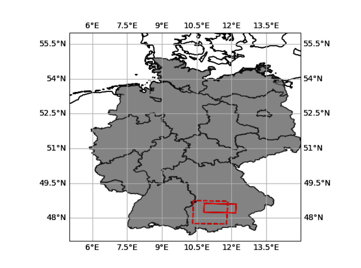
Figure 3: AOI in Germany. Solid lines denote the annotated AOI while dashed lines denote the area covered by DEU-base and DEU-time pre-training data.

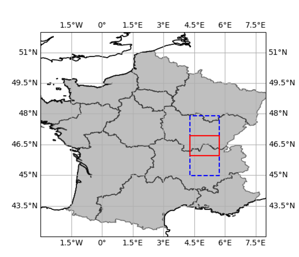
Figure 4: AOI in France. Solid lines denote the annotated AOI while dashed blue lines denote the area covered by FRA-space pre-training data. FRA-base and FRA-time datasets cover the same AOI as the annotated dataset.

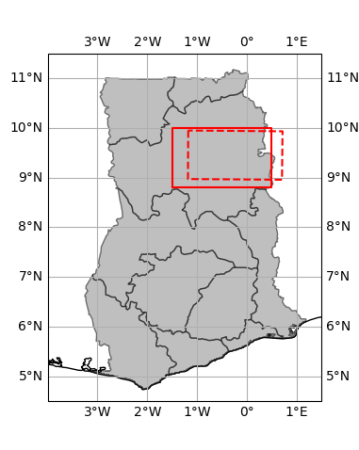
Figure 5: AOI in Ghana. Solid lines denote the annotated AOI while dashed lines denote the area covered by GHA-base pre-training data.

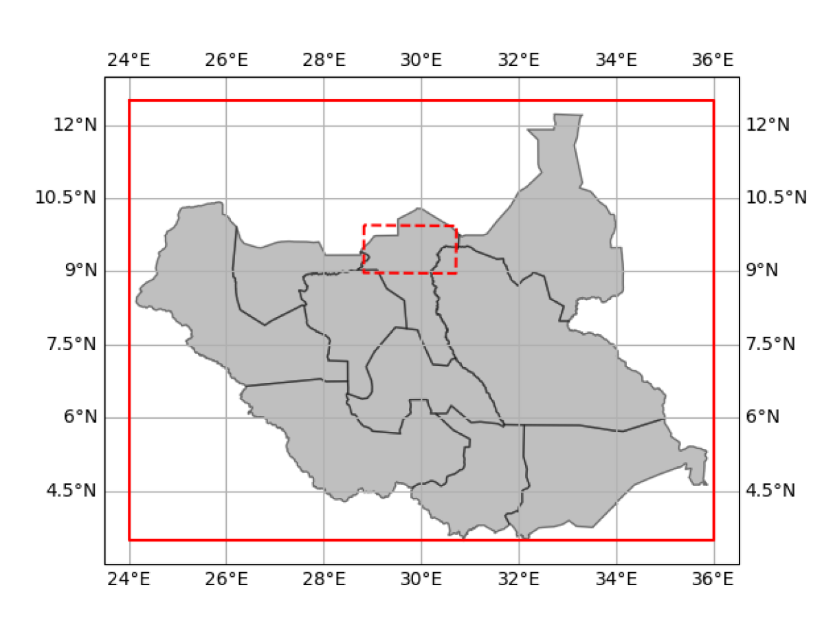
Figure 6: AOI in S.Sudan. Solid lines denote the annotated AOI while dashed lines denote the area covered by SSU-base and SSU-time pre-training data.

Experiments are performed with publicly available data from four different AOI in Germany (DEU), France (FRA), Ghana (GHA) and S.Sudan (SSU). Annotated data were obtained from the original studies. For downloading and extracting data without annotations for self-supervised training we use the DeepSatData pipeline [59]. The choice of sample dimensions for the pre-training datasets (Table I) was motivated by the sample size of the segmentation datasets (Table II). It was desired that random crops during pre-training match the size of the respective segmentation datasets while maintaining balance between two desired properties: the need for enough ovelap between crops to obtain positive pairs and enough stochasticity when extracting different views. Samples for all datasets are square images.

In France we use the same training data as [24] but keep only 13 out of the 166 available land cover types (PPH, J6S, SNE, ORH, PRL, PTC, MH7, RDF, BOP, MLG, RVI, MIS, TRE) and only for year 2018. This choice was made on the basis of retaining the most numerous and best performing classes. This dataset is completely covered by S2 tile T31TFM. The FRA-base dataset consists of S2 tile T31TFM for year 2018, while the FRA-time dataset extends that for years 2016 and 2017. The FRA-space dataset consists of tiles T31TFN, T31TFM and T31TFL for year 2018. In Germany we use the data from [47] for year 2016 keeping all 17 crop type groupings (maize, wheat, meadow, winter barley, potato, rapeseed, summer barley, hop, triticale, oat, rye, sugar beet, spelt, aparagus, beans, peas, soybeans) from the original study. The DEU-base dataset consists of tile T32UPU for year 2016 while the DEU-time dataset extends that with images from years 2017 and 2020.
Both datasets in Europe contain all 13 Sentinel-2 bands plus an additional day of year (doy) parameter indicating the day of the year normalized in $(0,1]$. Subsampling was performed uniformly in space such that even the smallest datasets cover the entire AOI. The locations of data for Germany and France are shown in Figs.4, 4.

For experiments in Africa we used the Ghana and South Sudan datasets from [48] shared by the Radiant Earth Foundation. For Ghana we selected the 4 most popular crop types found in the AOI (ground nut, maize, rice and soy bean). The training and evaluation data span the 2016 growing season. The GHA-base dataset consists of tile T31PZR for year 2016. In South Sudan we selected 6 land cover types out of the most populated land cover types found in the data (bush, bare soil, forest, shrubland, grasslands and meadows, wetland) for the 2017 growing season. The SSU-base dataset consists of tile T35PMK for 2017 while the SSU-time dataset extends that to years 2018 and 2020. Data in Ghana cover a relatively small AOI while data in South Sudan cover a very large AOI which spans the entire country. Both datasets are quite sparse both in terms of parcel locations (the average distance between parcels is large) but also in terms of ratio of foreground to total number of pixels (few foreground pixels w.r.t. total). The locations of data for Ghana and South Sudan are shown in Figs.6, 6. Both African datasets contain 10 Sentinel-2 bands plus an additional doy parameter. We note that in order to protect privacy both datasets do not include information on the location of agricultural parcels. As such splitting the data into train and evaluation sets was performed randomly in space while ensuring that all datasets maintain an equal ratio from every class. We also note that for privacy preservation purposes the input satellite images in both datasets include some random noise component making them sub-optimal for image classification purposes.

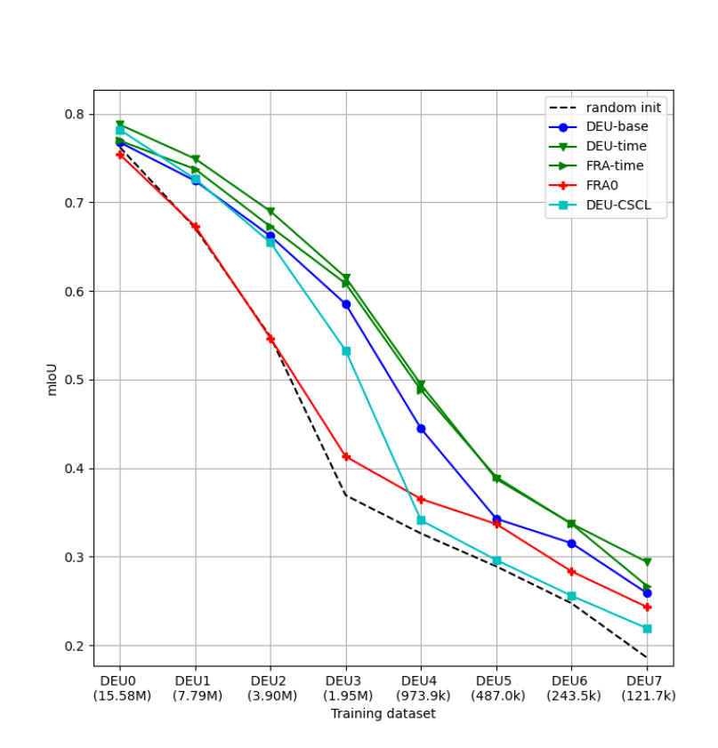
Figure 7: Germany - mIoU at evaluation set.

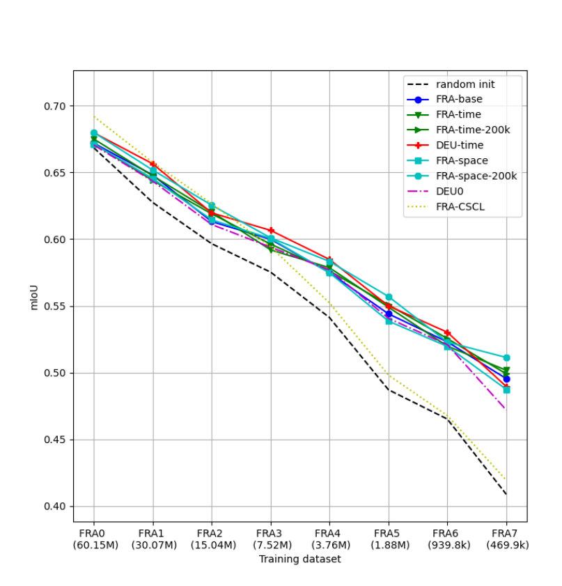
Figure 8: France - mIoU at evaluation set.

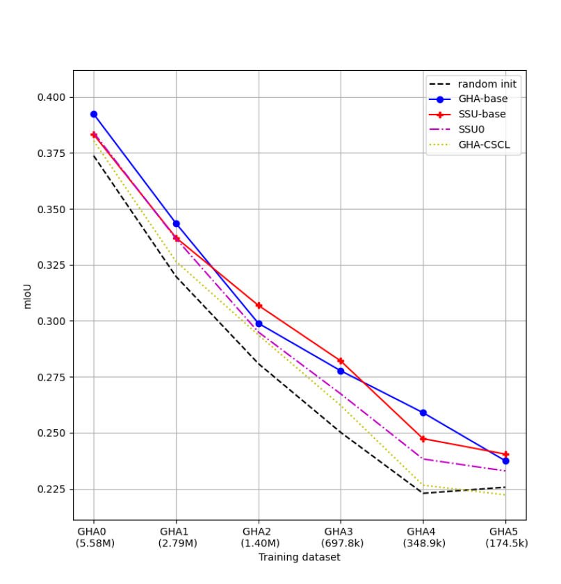
Figure 9: Ghana - mIoU at evaluation set.

Figure 10: S.Sudan - mIoU at evaluation set.

IV-B Training implementation details

For all experiments we used the UNet3Df models from [24]. This model is a variation of UNet3D [51] - previously used for land cover semantic segmentation in [48, 24] - better suited for metric style learning. We refer the reader to [24] for further details. This model was preferred to Conv-RNN alternatives because it is faster to train thus, more suitable for use in multiple experiments. All models were trained using commodity Nvidia TITAN Xp and RTX 2080 gpus. A single card was used for training the final segmentation models. For pre-training two gpus were used in a data parallel fashion, however, the model can be pre-trained using a single gpu and this choice was employed to increase training speed rather than to overcome limitations imposed by accelerator memory. Further details can be found in Appendix B.

IV-C Comparison with random initialization

We present a comparison between models starting with random parameter initialization and those pre-trained using the base datasets. Results are presented in Figs.8, 8, 10, 10 respectively for Germany, France, Ghana and S.Sudan. Overall, as expected, we observe evaluation performance to drop with decreasing number of samples in the training datasets. Additionally, pre-trained models are shown to outperform their counterparts in every case tested with no exception. From the horizontal distances between the pre-trained and random initialization curves it appears that pre-training has an equivalent effect with doubling the amount of training data. There is a general trend for pre-training to have a more significant benefit in the smaller annotation space. However, that is not always the case. For example in Germany performance seems to improve more on medium size (DEU3, DEU4) rather than the smallest datasets. We also note that pre-training performance gains are smaller on the African datasets. Potential reasons could be the inclusion of noise in the training datasets which introduces a gap between pre-training and training data or the large cloud cover which affects both pre-training and final segmentation training.

IV-D Comparison with state-of-the-art pre-training

We compare EmbeddingEarth with the recently proposed CSCL method [24] for supervised visual pre-training. While our method does not require ground truths for the pre-train task CSCL depends on provided annotations. As such, to ensure a fair comparison, CSCL pre-trained models only use the amount of annotations available in each training set, e.g. FRA2 segmentation model is initialized by a model pre-trained on FRA2. Results are presented in Figs.8, 8, 10, 10 respectively for Germany, France, Ghana and S.Sudan. We observe decreasing performance gains for CSCL in smaller size datasets which is expected given that the size of the pre-training set matches the training set size. Our method exhibits a much gentler performance degardation w.r.t. the dataset size and outperforms CSCL in every case apart from the largest datasets for France (FRA0-FRA2).

IV-E Analysis of results

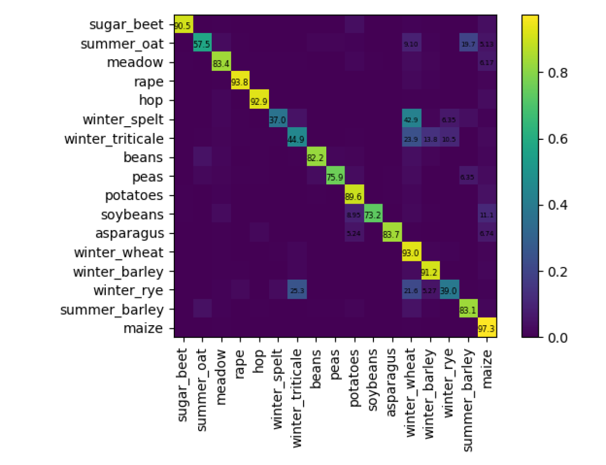
(a) DEU1-random

(b) DEU1-pretrain

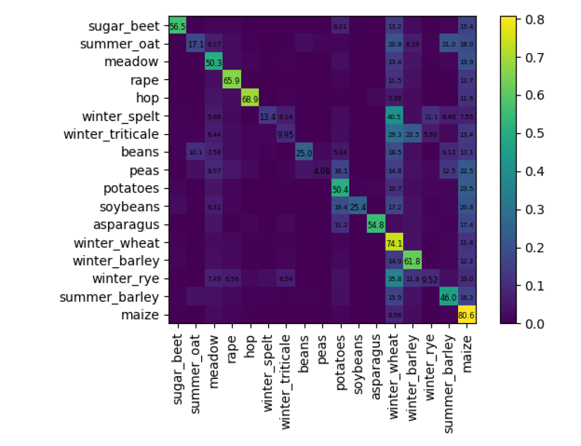
(c) DEU4-random

(d) DEU4-pretrain

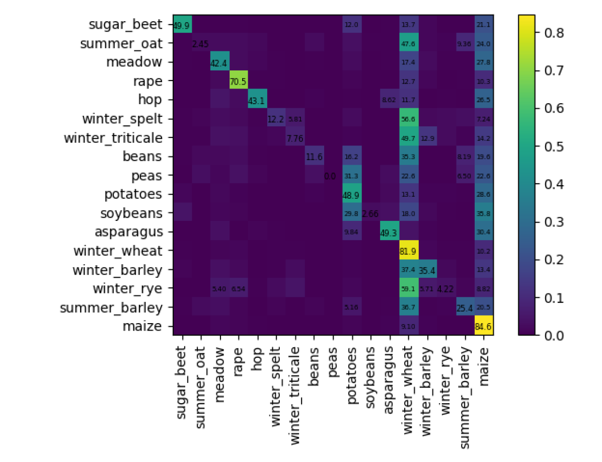
(e) DEU6-random

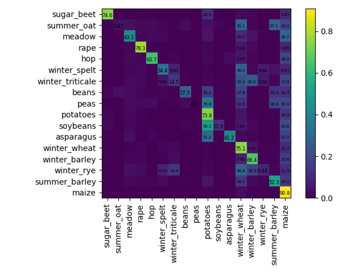
(f) DEU6-pretrain

Figure 17: Germany - Confusion matrices at evaluation set. From top to bottom: DEU1, DEU4, DEU6 training datasets, left to right: random and pre-trained initialization. Better viewed in color and zoomed in.

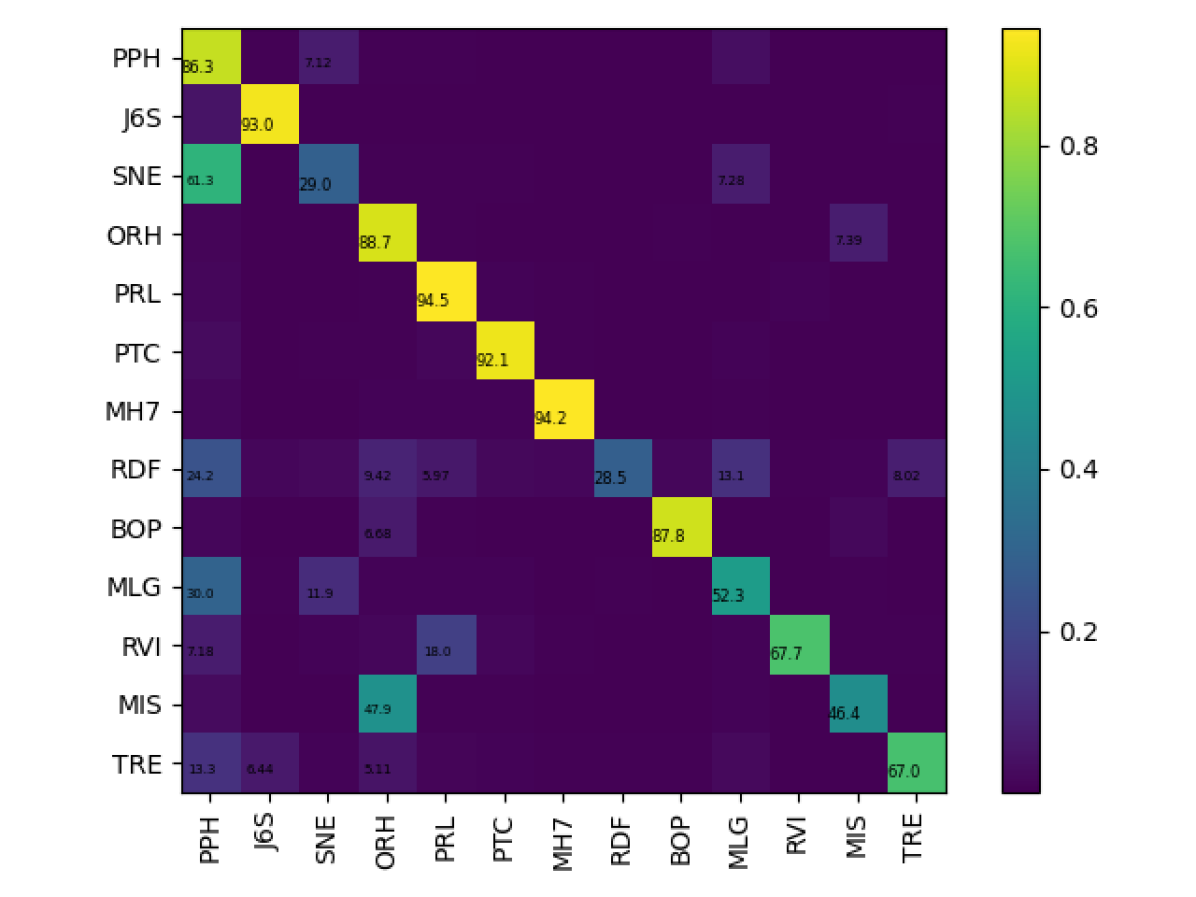
(a) FRA1-random

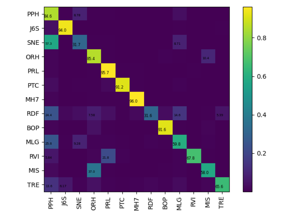
(b) FRA1-pretrain

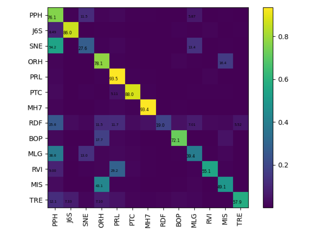
(c) FRA4-random

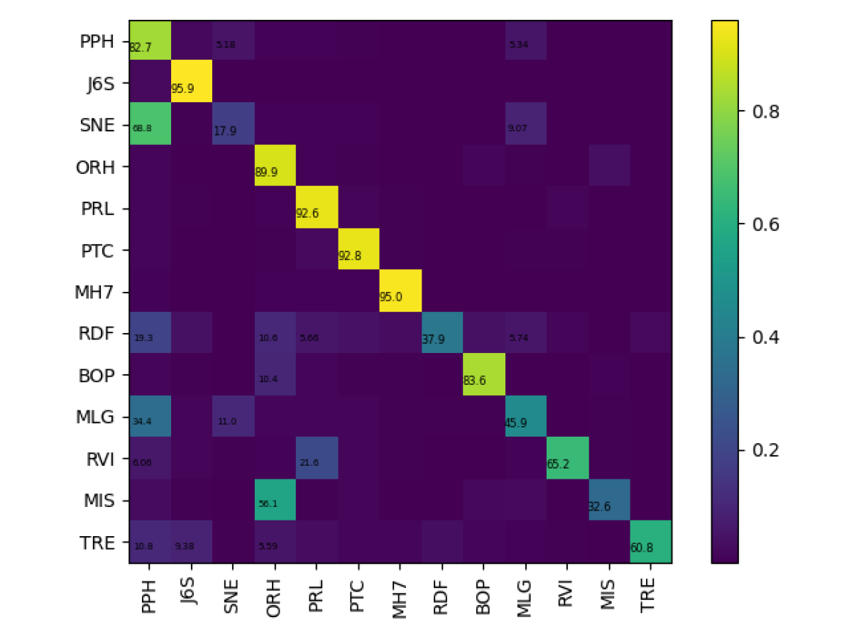
(d) FRA4-pretrain

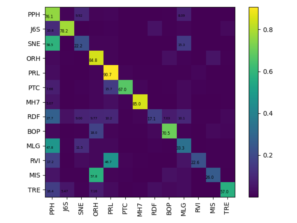
(e) FRA6-random

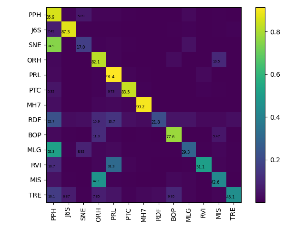
(f) FRA6-pretrain

Figure 18: France - Confusion matrices at evaluation set. From top to bottom: FRA1, FRA4, FRA6 training datasets, left to right: random and pre-trained initialization. Better viewed in color and zoomed in.

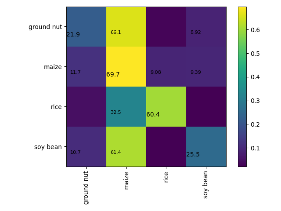
(a) GHA1-random

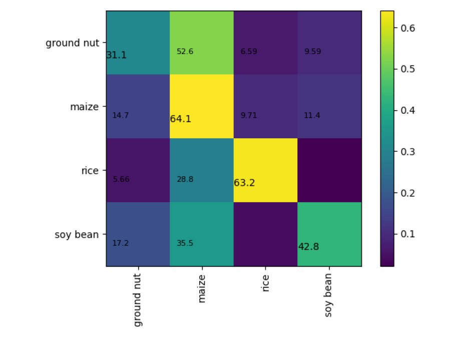
(b) GHA1-pretrain

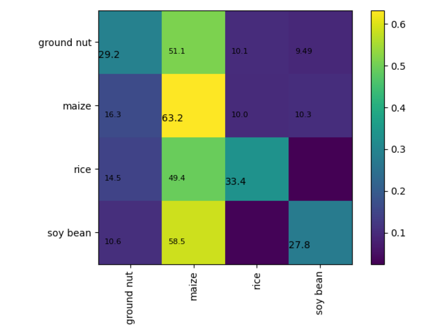
(c) GHA3-random

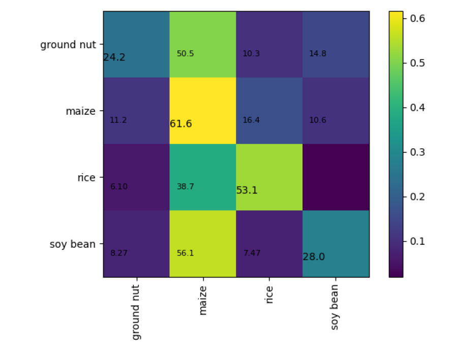
(d) GHA3-pretrain

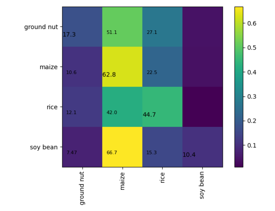
(e) GHA5-random

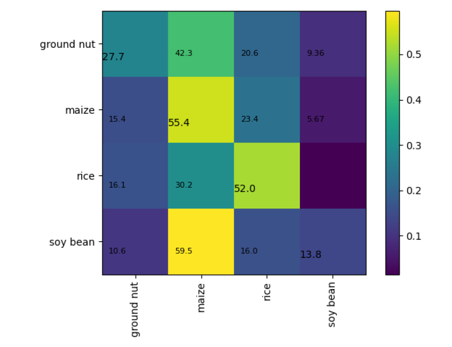
(f) GHA5-pretrain

Figure 19: Ghana - Confusion matrices at evaluation set. From top to bottom: GHA1, GHA3, GHA5 training datasets, left to right: random and pre-trained initialization. Better viewed in color and zoomed in.

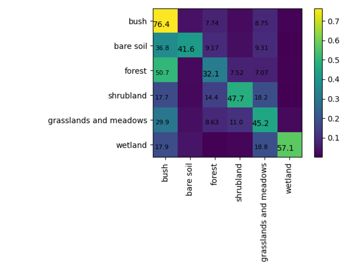
(a) SSU1-random

(b) SSU1-pretrain

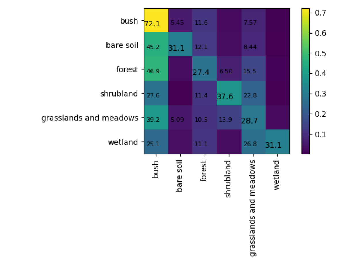
(c) SSU3-random

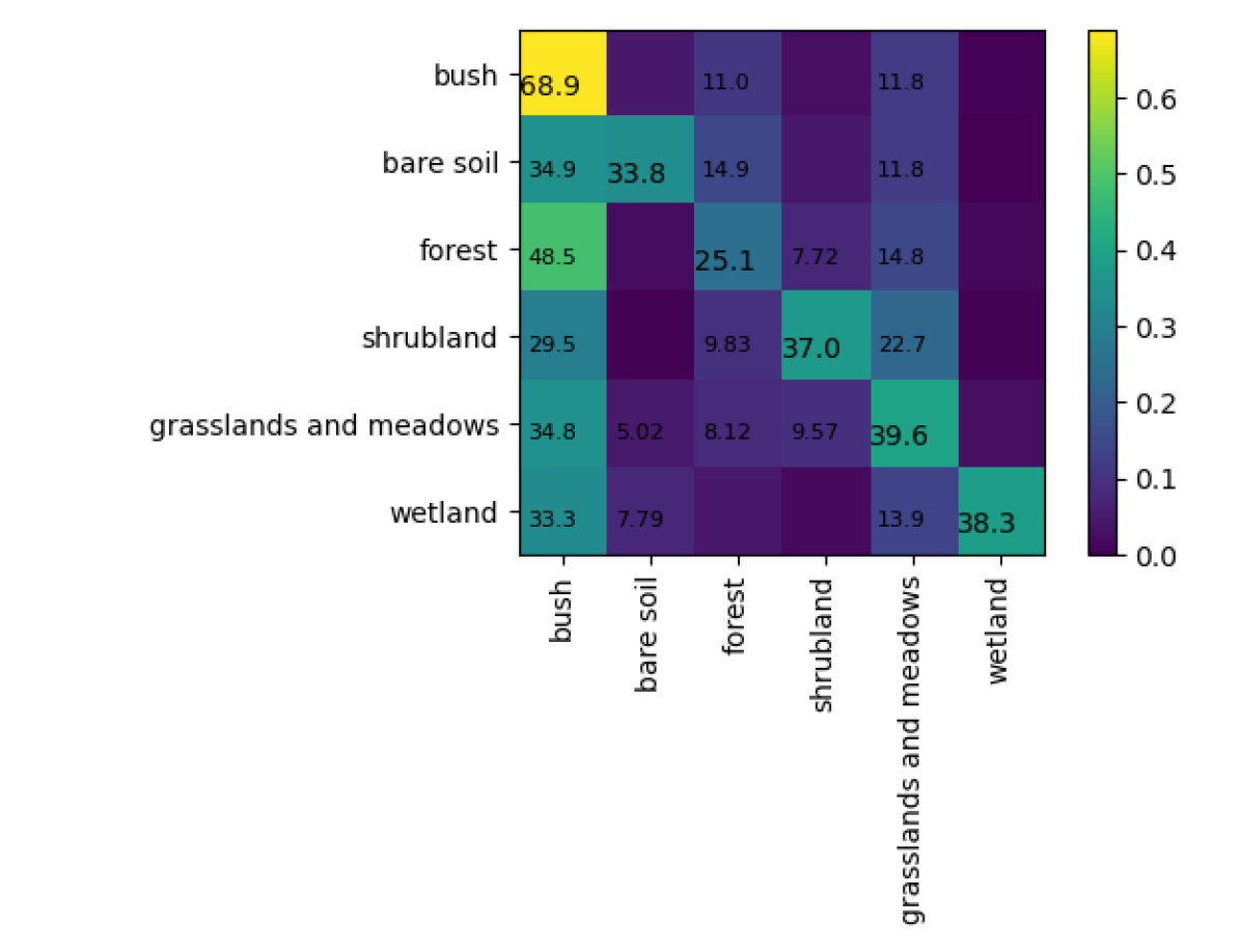
(d) SSU3-pretrain

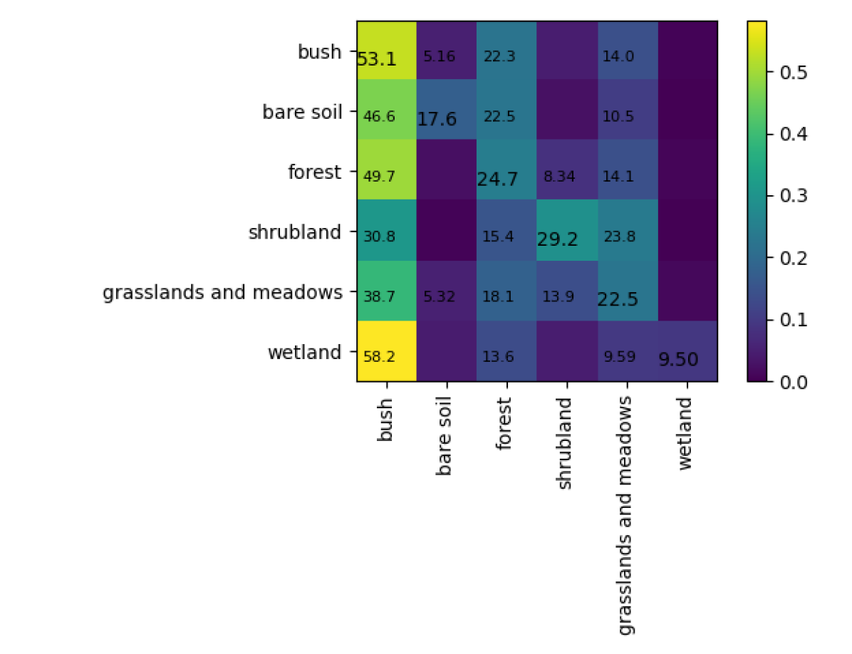
(e) SSU5-random

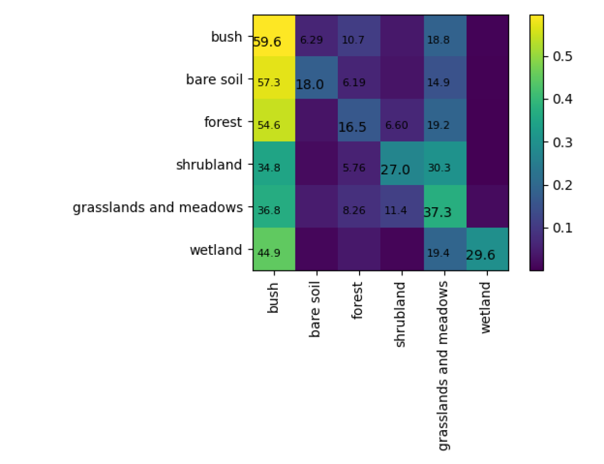
(f) SSU5-pretrain

Figure 20: S.Sudan - Confusion matrices at evaluation set. From top to bottom: SSU1, SSU3, SSU5 training datasets, left to right: random and pre-trained initialization. Better viewed in color and zoomed in.

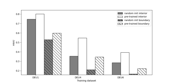
Figure 21: Germany - mIoU at evaluation set. Comparison between random initialization and pre-training for interior and boundary pixels.

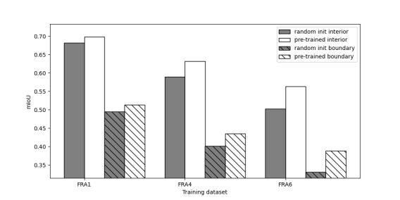
Figure 22: France - mIoU at evaluation set. Comparison between random initialization and pre-training for interior and boundary pixels.

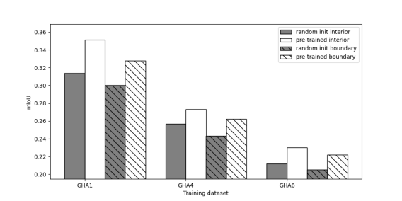
Figure 23: Ghana - mIoU at evaluation set. Comparison between random initialization and pre-training for interior and boundary pixels.

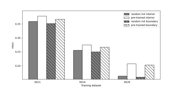
Figure 24: S.Sudan - mIoU at evaluation set. Comparison between random initialization and pre-training for interior and boundary pixels.

We find that improvements are generally evenly distributed among classes and pixel location within a parcel. In Fig.11 we show confusion matrices for the DEU4 dataset and compare per class performance for random initialization of parameters and DEU-base pre-training. Similar confusion matrices for all countries can be found in Figs.17, 18, 19, 20 in Appendix C. We observe improvements for all classes in Germany and the majority of classes elsewhere. In France Ghana and S.Sudan there are few classes for which random initialization performs better, however, overall improvement is always higher for the pre-trained models. We also distinguish between performance improvement at parcel interior vs boundary locations. For this purpose a boundary location is assumed to be any location which does not share the same class as all of its $3\times 3$ local neighbourhood. Results are plotted in Fig.12 for Germany. Additional plots for all countries can be found in Figs.21, 22, 23, 24 in Appendix C. We observe similar improvement at both interior and boundary locations which is different from the findings of [24] whose pre-training task lead to greater performance gains at the boundaries.

(a) random init

(b) DEU-base pre-train

Figure 11: Germany - Confusion matrices at evaluation set for (a) random and (b) pre-trained initializations. Models trained using the DEU4 dataset.

Figure 12: Germany - mIoU at evaluation set. Comparison between random initialization and pre-training for interior and boundary pixels.

IV-F Ablation studies

In this section we present results from a series of ablation studies to asses how various qualities of the pre-training affect final segmentation performance.

Figure 13: Ablation on $\tau$ parameter (eq. 1) in France. All models were pretrained using the FRA-base dataset.

For deciding on a value for the temperature scaling parameter $\tau$ (eq. 1) we explore how various $\tau$ values affect performance. We test typically used values close to $0.07$ used in the original implementation of MoCo [39]. Results are shown in Fig.13. Overall most temperature parameter values appear to lead to similar performance on semantic segmentation apart from $\tau=0.03$ which seems to significantly lag on smaller size datasets. The choice of $\tau=0.10$ for the remaining experiments was made because this parameter was found to be a good performer in most cases and is close to the values typically used in MoCo.

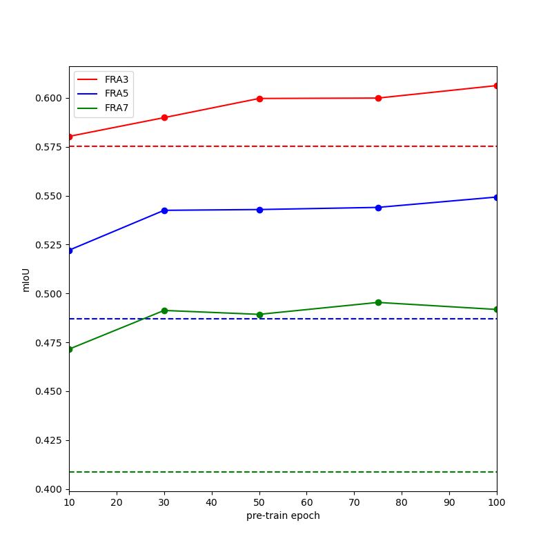
Figure 14: France - mIoU at evaluation set. Segmentation performance by sampling initialization points during pre-training. Dashed lines indicate random initialization baselines.

It is of interest to find what is the optimum number of pre-training steps. To find out we are sampling initialization values at various stages during pre-training and compare downstream segmentation performance. Results are presented in Fig.14. Overall we observe that even minimal pre-training for $10$ epochs improves over random initialization in every case and performance continues to improve with more pre-training. This suggests that the selected number of $100$ epochs might be sub-optimal and more steps could lead to better performance in practice.

Next we want to assess the generality of pretrained features. By mixing pre-training and finetuning regions we assess the importance of pre-training at a different location than that of the downstream task. More specifically we swap the initializations between each set of countries in Europe and Africa. Results using the swaped datasets for Germany, France, Ghana and S.Sudan can be seen in Figs.8, 8 and Figs.10, 10. We find that swapping locations has little to no effect over downstream segmentation performance and in numerous cases we obtain improved performance using an initialization point from a different country. This suggests that the reason our pre-training scheme improves performance is not just because the network learns the instance discrimination task for a particular region. This is also in contrast with the tendency of fully supervised land cover segmentation models not to generalize to completely new regions. To our knowledge this is the first method exhibiting that quality. More importantly it opens the possibility to pre-train and collect a set of initialization values for popular land cover identification models and use these instead of random initialization for downstream tasks. This method has been very successfully applied to other computer vision problems such as object detection and semantic segmentation using ImageNet [12] pre-trained initializations for faster training and improved performance.

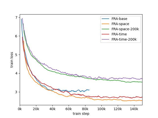
Figure 15: France. Train loss during pre-training.

So far we have seen that we get stronger improvements compared to the randomly initialized baselines for small size training datasets. In a similar spirit, here we assess the significance of the size of pre-training datasets in segmentation performance. We compare the results obtained using the base datasets with the time and space datasets from Table I. Additionally, we want to asses the relative importance of using more locations for a given period of time compared to a longer period for a given set of locations. Results are presented in Figs.8, 8. We note a general trend for time pre-trained models to outperform both base and space pre-trained ones when using the default 67k data queue. Using a larger pre-training AOI does not appear to offer any benefits and models pre-trained with FRA-space are in most cases outperformed by FRA-base models. This indicates that pre-training over a larger AOI than that of the training set (Fig.4) can hinder downstream model performance. However, it was previously shown that pre-training at a different location does not affect performance which raises the question why using a pre-train dataset covering larger regions does not offer any improvement. One reason could be that the size of the examined datasets is already large enough to achieve most of the benefits of pre-training. Another possibility is that the larger the area covered by a pre-training dataset the easier the objective function becomes to optimize as queue encodings correspond to increasingly disparate locations and are easier to distinguish from the query vectors. We present some empirical evidence towards the latter reason in Fig.15 where we plot the train loss for pre-training in France and observe lower values for the FRA-space dataset consistently during training indicating an easier optimization objective. Furthermore, we perform pre-training by tripling the size of the data queue to size 201k. Increasing the size of the queue introduces a tradeoff between including more diversity in the negative samples and increasing the duration (in training steps) an encoding spends in the queue. More diversity is achieved simply because encodings from more locations are included in the queue and thus as negative pairs in the loss function (eq.1). The number of negative pairs has been previously shown to improve the quality of learnt features is contrastive learning [39, 27]. However, increasing the duration an encoding spends in the data queue means that currently encoded queries are being compared with encodings from earlier instantiations of the keys encoder which might not be as relevant during the current training step. In our case training with a 201k data queue is found to be a more difficult pre-training optimization objective (Fig.15). From Fig.8 we observe an improvement in performance for the space dataset but not for the time dataset.

We have shown the benefits of the proposed pre-training scheme w.r.t. random initialization. Another option is to use a previously trained supervised land cover segmentation model as an initialization point for a new region. To recreate a realistic scenario in which we have a large labelled dataset in a source country and we want to train for a target country we use the best model trained with the largest dataset in each respective country, i.e. DEU0, FRA0, GHA0, SSU0, as the initialization for another country in the same continent. Results are shown in Figs.8, 8, 10, 10. In all cases self-supervised initializations outperform the fully supervised ones. In terms of the observed differences the results are mixed. For Germany and S.Sudan the differences with self-supervision are significant, the fully supervised initializations are closer to the random rather than the self-supervised ones. For France and Ghana the differences are not as significant.

In most cases, we observe a smaller benefit of supervised pre-training over random initialization for the larger training datasets and some benefit for the smaller datasets. An exception to pattern is Ghana in which the benefit is almost constant for all dataset sizes.

V Conclusion

In this paper we presented a self-supervised pre-training methodology for land cover semantic segmentation tasks using time series of satellite images. To assess the merits of our approach we performed a large scale study using Sentinel-2 images from four countries in Europe and Africa. In every case tested we found significant improvements up to $+25\%$ absolute mIoU over random initialization and showed improvements over fully supervised pre-training. Additionally we have shown that the learnt features generalize equally well to unseen regions significantly improving downstream segmentation performance in different countries than the ones used during pre-training. Because of this we see our work opening a new direction in land cover segmentation making it possible to use a set of pre-trained model weights for high performing segmentation models as initialization points for EO related downstream tasks similar to how pre-trained models have been used in computer vision tasks. The Embedding Earth pretext task does not use any annotations, thus, it is not in any way restricted to learning a particular type or land cover but is a system for extracting features characteristic of the spatiotemporal patterns of the input image time series. As a result, although not tested in tasks other than land cover segmentation, we expect pre-trained initialization points to be beneficial for other EO tasks including but not limited to dense classification such as object detection and dense regression. We leave these possibilities as a topic for future research.

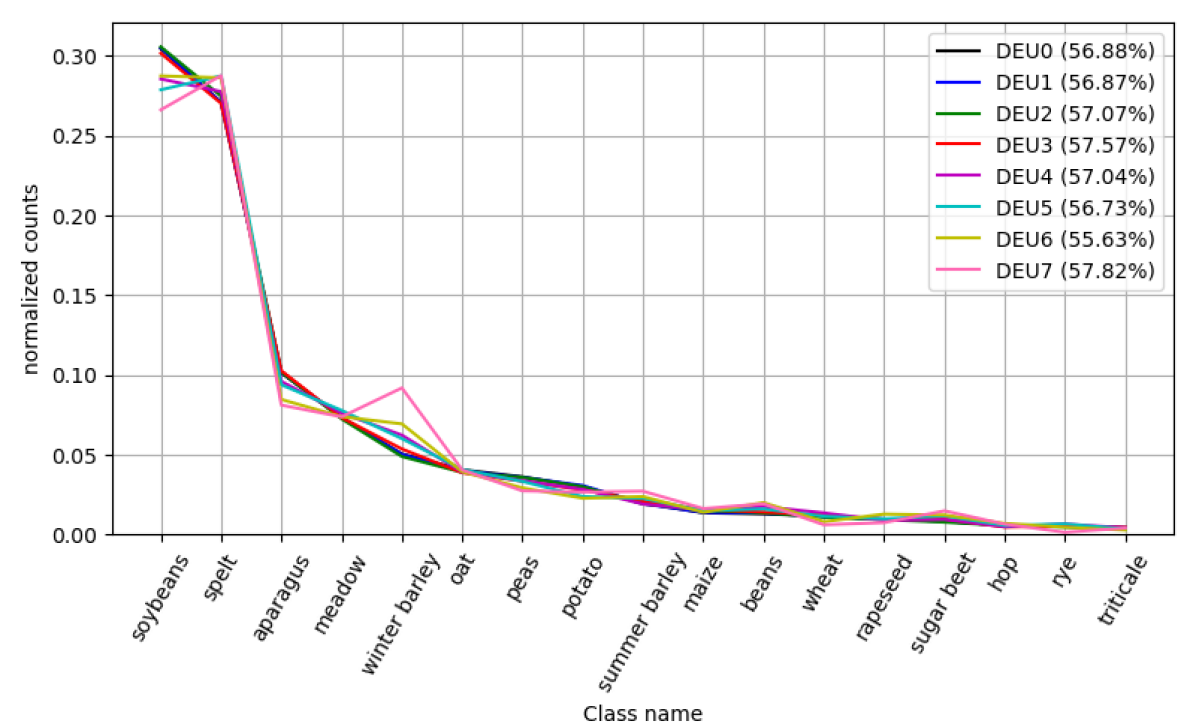
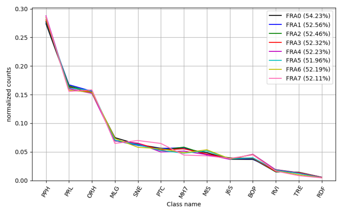
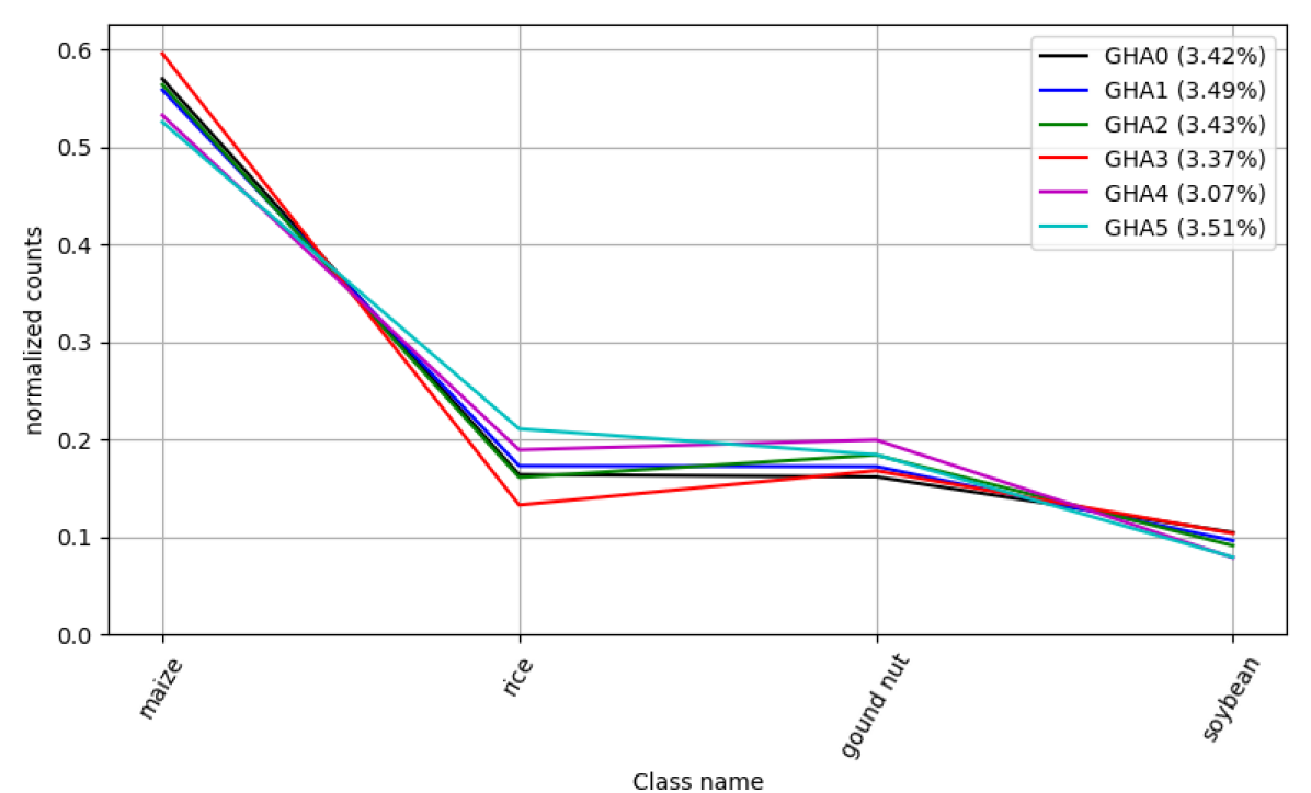
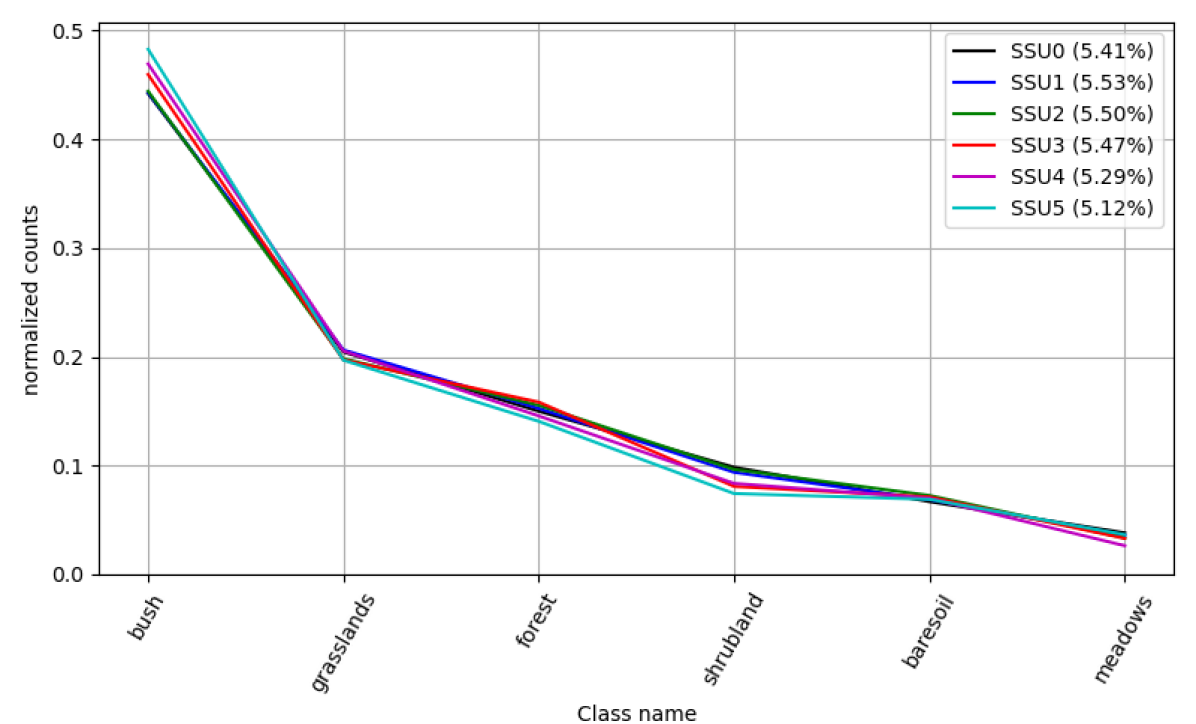
Figure 16: Class distribution among the training datasets. (top-left) Germany, (top-right) France, (bottom-left) Ghana, (bottom-right) S.Sudan. $\%$ in legend parentheses is the ratio of foreground to overall pixels for each dataset.

Appendix A Dataset class distributions

In Fig.16 we present normalized pixel counts (pixel count for each class divided by total) for all training datasets in the four countries tested. By design we maintain a similar distribution of pixel counts is maintained for all datasets in each country. Only smaller size datasets exhibit some limited variation from the average distribution which can be attributed to their limited size, i.e. winter barley in DEU7. In the legend we also show the ratio of foreground to overall pixels for each dataset. Note how this value is significantly lower for the Arican compared to the European datasets as a result of the data sparsity in Ghana and S.SUdan.

Appendix B Training implementation details

Pre-training details. All models were pre-trained using the SGD optimizer with momentum $0.9$ and a learning rate $0.0001$ reduced by $\times 10$ at epochs $40$ and $60$. Unless otherwise indicated the temperature parameter for eq.1 is set to $0.10$, the size of the keys queue is set to $67,200$ and we always sampled $32$ pixels in correspondence between views to use as positive pairs. The batch size was set to $60$ for datasets in Europe and $30$ for datasets in Africa. All models were pre-trained for $100$ epochs in Europe and $200$ epochs in Africa. We chose to train for more epochs in Africa because the number of samples in the pre-training set was reduced as a consequence of the larger sample size ($100$ pixels compared to $48$ for France and $32$ for Germany). The crop size during pre-training was selected such that it matched the sample size of the respective segmentation dataset. France is an exception to this rule as models there were pre-trained with crop size $32$ while the dataset from [24] contains samples of size $48$. We have empirically found this not to be significant for final segmentation performance as there are cases where models pre-trained in Germany with much smaller crop size outperform models pre-trained in France. Segmentation training details. All models were trained using the Adam optimizer [60] with default hyperparameters $\beta_{1}=0.9,\beta_{2}=0.999$ and a learning rate $0.0001$ reduced exponentialy at a rate of $0.975$ every two epochs. Details on the total number of epochs and batch sizes used can be found in Table III. In all cases training hyperparameters were kept constant between runs using the same dataset, e.g. all models trained with the FRA1 dataset use the same training protocol.

train set	N epochs	batch size
DEU0-3	150	32
DEU4-5	225	16
DEU6-7	225	8
FRA0-3	150	32
FRA4-5	225	16
FRA6-7	225	8
GHA0	400	16
GHA1-5	400	8
SSU0-1	300	16
SSU2-5	400	8

Table III: Segmentation training. Number of epochs and batch size.

Appendix C Detailed evaluation metrics

Tables IV, VI, V, VII show detailed evaluation metrics for all runs in Germany, Ghana, France and S.Sudan. We present macro (averaged over classes) accuracy, mIoU and F1 scores and micro (averaged over pixels) accuracy and mIoU. Figs.17, 18, 19, 20 show confusion matrices for Germany, France, Ghana and S.Sudan respectively. All values of the diagonal are displayed. To avoid cluttering non diagonal values are only displayed if they are greater than $0.05$. Figs. 21, 22, 23 24 present a performance comparison between random and pre-trained initialization for object interior and boundary pixels for Germany, France, Ghana and S.SUdan.

datasets		macro			micro
pre-train	train	acc	iou	F1	acc	iou
-	DEU0	0.8377	0.7623	0.8524	0.9261	0.8624
DEU-base	DEU0	0.8435	0.7677	0.8566	0.9233	0.868
DEU-time	DEU0	0.8625	0.7877	0.8717	0.9341	0.8763
FRA-time	DEU0	0.8537	0.7696	0.8597	0.9291	0.8676
$FRA0^{*}$	DEU0	0.8289	0.7540	0.8463	0.9218	0.8549
DEU0†	DEU0	0.8588	0.7819	0.8667	0.9334	0.8755
-	DEU1	0.7535	0.6710	0.7810	0.8956	0.8105
DEU-base	DEU1	0.8058	0.7243	0.8225	0.9160	0.8449
DEU-time	DEU1	0.8286	0.7492	0.8422	0.9228	0.8567
FRA-time	DEU1	0.8184	0.7375	0.8349	0.9176	0.8477
FRA0	DEU1	0.7719	0.6731	0.7867	0.8925	0.8058
DEU1†	DEU1	0.811	0.7264	0.8249	0.9173	0.8472
-	DEU2	0.6740	0.5482	0.6819	0.8341	0.7154
DEU-base	DEU2	0.7476	0.6620	0.7745	0.8952	0.8103
DEU-time	DEU2	0.7848	0.6900	0.7948	0.9043	0.8254
FRA-time	DEU2	0.7616	0.6726	0.7816	0.8978	0.8146
FRA0	DEU2	0.6546	0.5467	0.6851	0.8278	0.7062
DEU2†	DEU2	0.751	0.6546	0.767	0.8935	0.8075
-	DEU3	0.4904	0.3692	0.5137	0.6977	0.5358
DEU-base	DEU3	0.6910	0.5851	0.7100	0.8631	0.7592
DEU-time	DEU3	0.7050	0.6152	0.7320	0.8766	0.7804
FRA-time	DEU3	0.7028	0.6083	0.7312	0.8691	0.7685
FRA0	DEU3	0.5305	0.4130	0.5609	0.7309	0.5796
DEU3†	DEU3	0.6416	0.5326	0.6621	0.8422	0.7274
-	DEU4	0.4292	0.3261	0.4611	0.6730	0.5072
DEU-base	DEU4	0.5440	0.4446	0.5733	0.7578	0.6516
DEU-time	DEU4	0.5920	0.4943	0.6198	0.8206	0.6957
FRA-time	DEU4	0.5904	0.4880	0.6201	0.8056	0.6745
FRA0	DEU4	0.4673	0.3651	0.5016	0.7132	0.5542
DEU4†	DEU4	0.4372	0.341	0.4729	0.7068	0.5466
-	DEU5	0.4042	0.289	0.4150	0.6377	0.4682
DEU-base	DEU5	0.4403	0.3428	0.4774	0.6969	0.5358
DEU-time	DEU5	0.4961	0.3877	0.5217	0.7350	0.5711
FRA-time	DEU5	0.4849	0.3898	0.5243	0.7269	0.5710
FRA0	DEU5	0.4208	0.3368	0.4678	0.6991	0.5374
DEU5†	DEU5	0.3889	0.2962	0.4481	0.6546	0.4866
-	DEU6	0.3369	0.2473	0.3853	0.6254	0.4528
DEU-base	DEU6	0.4171	0.3152	0.4419	0.6781	0.5129
DEU-time	DEU6	0.4441	0.3372	0.4888	0.7057	0.5453
FRA-time	DEU6	0.4315	0.3370	0.4732	0.7108	0.5514
FRA0	DEU6	0.364	0.2833	0.4250	0.6727	0.5068
DEU6†	DEU6	0.3493	0.2558	0.3899	0.6513	0.4829
-	DEU7	0.2818	0.1861	0.3361	0.5779	0.4063
DEU-base	DEU7	0.3514	0.2589	0.3694	0.6553	0.4873
DEU-time	DEU7	0.3820	0.2940	0.4230	0.6540	0.4854
FRA-time	DEU7	0.3517	0.2670	0.4012	0.6502	0.4817
FRA0	DEU7	0.3331	0.2432	0.3687	0.6471	0.4783
DEU7†	DEU7	0.3007	0.2192	0.3831	0.6228	0.4522

Table IV: Results in Germany. * supervised pre-training, $\dagger$ CSCL pre-training [24]

datasets		macro			micro
pre-train	train	acc	iou	F1	acc	iou
-	FRA0	0.7592	0.6685	0.7733	0.8333	0.7142
FRA-base	FRA0	0.7647	0.6720	0.7766	0.8345	0.7158
FRA-time	FRA0	0.7633	0.6751	0.7769	0.8352	0.7230
FRA-time*	FRA0	0.7668	0.6716	0.7777	0.8307	0.7104
FRA-space	FRA0	0.7652	0.6714	0.7763	0.8344	0.7159
FRA-space*	FRA0	0.7620	0.6800	0.7848	0.8373	72.01
DEU-time	FRA0	0.7646	0.6798	0.7810	0.8349	0.7241
DEU0	FRA0	0.7540	0.6706	0.7719	0.8312	0.7236
FRA0†	FRA0	0.773	0.692	0.7913	0.8421	0.7273
-	FRA1	0.7292	0.6275	0.7394	0.8069	0.6773
FRA-base	FRA1	0.7498	0.6481	0.7585	0.8158	0.6889
FRA-time	FRA1	0.7452	0.6475	0.7552	0.823	0.6992
FRA-time*	FRA1	0.7482	0.644	0.756	0.7116	0.683
FRA-space	FRA1	0.7327	0.6454	0.7561	0.8172	0.6909
FRA-space*	FRA1	0.754	0.6518	0.7619	0.8173	0.691
DEU-time	FRA1	0.7487	0.6565	0.7639	0.8265	0.7043
DEU0	FRA1	0.7373	0.6435	0.7514	0.8106	0.6837
FRA1†	FRA1	0.7515	0.6575	0.7611	0.8221	0.698
-	FRA2	0.7008	0.5966	0.7089	0.7826	0.6469
FRA-base	FRA2	0.6878	0.581	0.6999	0.7811	0.6408
FRA-time	FRA2	0.7294	0.6205	0.7363	0.7997	0.6630
FRA-time*	FRA2	0.7301	0.619	0.7289	0.7858	0.6502
FRA-space	FRA2	0.718	0.6145	0.7303	0.7930	0.6570
FRA-space*	FRA2	0.7338	0.6255	0.739	0.7941	0.6582
DEU-time	FRA2	0.7212	0.6197	0.7349	0.7977	0.6619
DEU0	FRA2	0.7127	0.6110	0.7232	0.7840	0.6483
FRA2†	FRA2	0.7229	0.6266	0.7369	0.8066	0.6759
-	FRA3	0.6713	0.5753	0.6941	0.7760	0.6339
FRA-base	FRA3	0.6931	0.5999	0.7167	0.7948	0.6595
FRA-time	FRA3	0.6873	0.5920	0.7092	0.7899	0.6528
FRA-time*	FRA3	0.703	0.5963	0.7159	0.7758	0.6337
FRA-space	FRA3	0.7000	0.6005	0.7201	0.7852	0.6463
FRA-space*	FRA3	0.7004	0.601	0.718	0.7888	0.6499
DEU-time	FRA3	0.7093	0.6066	0.7224	0.7823	0.6425
DEU0	FRA3	0.6951	0.5940	0.7104	0.7750	0.6343
FRA3†	FRA3	0.6862	0.5943	0.7091	0.7877	0.6498
-	FRA4	0.6426	0.5412	0.6632	0.7560	0.6077
FRA-base	FRA4	0.6767	0.5749	0.6973	0.7760	0.6340
FRA-time	FRA4	0.6835	0.5786	0.6992	0.7796	0.6388
FRA-time*	FRA4	0.6837	0.5762	0.698	0.7738	0.6311
FRA-space	FRA4	0.6868	0.5748	0.6956	0.7748	0.6324
FRA-space*	FRA4	0.6874	0.5833	0.6994	0.7872	0.6505
DEU-time	FRA4	0.6986	0.5848	0.7053	0.7778	0.6364
DEU0	FRA4	0.6792	0.577	0.693	0.7783	0.6388
FRA4†	FRA4	0.6591	0.5522	0.675	0.7566	0.6086
-	FRA5	0.6027	0.4871	0.6055	0.7194	0.5611
FRA-base	FRA5	0.6457	0.5440	0.6692	0.7574	0.6096
FRA-time	FRA5	0.6540	0.5490	0.6694	0.7916	0.6154
FRA-time*	FRA5	0.6584	0.5508	0.6747	0.7645	0.6188
FRA-space	FRA5	0.6456	0.5386	0.6617	0.7582	0.6101
FRA-space*	FRA5	0.6511	0.557	0.682	0.7602	0.615
DEU-time	FRA5	0.6512	0.5500	0.6726	0.7600	0.6230
DEU0	FRA5	0.6458	0.5407	0.6604	0.7561	0.6094
FRA5†	FRA5	0.6232	0.4981	0.6214	0.732	0.5799
-	FRA6	0.5701	0.4651	0.5924	0.7098	0.5501
FRA-base	FRA6	0.6402	0.5230	0.6497	0.7507	0.6009
FRA-time	FRA6	0.6269	0.5198	0.6439	0.7591	0.6117
FRA-time*	FRA6	0.6296	0.5255	0.6554	0.7408	0.5882
FRA-space	FRA6	0.6311	0.5196	0.6460	0.7311	0.5762
FRA-space*	FRA6	0.6278	0.5228	0.647	0.7233	0.6005
DEU-time	FRA6	0.6283	0.5302	0.6540	0.7545	0.6058
DEU0	FRA6	0.6218	0.5209	0.6406	0.7444	0.5942
FRA6†	FRA6	0.5646	0.4677	0.5921	0.7121	0.5577
-	FRA7	0.5360	0.4087	0.5354	0.6704	0.5227
FRA-base	FRA7	0.6038	0.4954	0.6253	0.7226	0.5656
FRA-time	FRA7	0.6061	0.5017	0.6280	0.7406	0.5881
FRA-time**	FRA7	0.6150	0.4990	0.6265	0.7351	0.5779
FRA-space	FRA7	0.5966	0.4874	0.6144	0.7210	0.5637
FRA-space**	FRA7	0.6268	0.5113	0.6393	0.7367	0.5831
DEU-time	FRA7	0.6036	0.4895	0.6138	0.7255	0.5693
DEU0	FRA7	0.5658	0.4719	0.5868	0.7269	0.5721
FRA7†	FRA7	0.5249	0.4193	0.5411	0.6936	0.531

Table V: Results in France. FRA-time** and FRA-space** pre-train datasets denote training with $201$k size queue. * supervised pre-training, $\dagger$ CSCL pre-training [24]

datasets		macro			micro
pre-train	train	acc	iou	F1	acc	iou
-	GHA0	0.5232	0.3737	0.5313	0.5977	0.4262
GHA-base	GHA0	0.5429	0.3923	0.5509	0.6441	0.4431
SSU-base	GHA0	0.5305	0.3832	0.5427	0.6152	0.4380
SSU0	GHA0	0.5373	0.3840	0.5466	0.6381	0.4401
GHA0†	GHA0	0.5228	0.3804	0.5363	0.6026	0.4312
-	GHA1	0.4554	0.3198	0.4663	0.5506	0.3799
GHA-base	GHA1	0.4960	0.3435	0.4958	0.5652	0.3939
SSU-base	GHA1	0.4765	0.3371	0.4881	0.5620	0.3919
SSU0	GHA1	0.4932	0.3367	0.4862	0.5596	0.3882
GHA1†	GHA1	0.4558	0.3265	0.4674	0.5542	0.3883
-	GHA2	0.4208	0.2809	0.4260	0.5065	0.3391
GHA-base	GHA2	0.4383	0.2989	0.4469	0.5362	0.3663
SSU-base	GHA2	0.4422	0.3069	0.4514	0.5437	0.3733
SSU0	GHA2	0.4357	0.2950	0.4406	0.5246	0.3556
GHA2†	GHA2	0.4367	0.2937	0.4388	0.525	0.3559
-	GHA3	0.3845	0.2502	0.3917	0.4795	0.3153
GHA-base	GHA3	0.4338	0.2777	0.4277	0.4908	0.3365
SSU-base	GHA3	0.4398	0.2821	0.4273	0.5126	0.3446
SSU0	GHA3	0.4008	0.2674	0.4105	0.5003	0.3336
GHA3†	GHA3	0.3978	0.2622	0.4074	0.4742	0.3108
-	GHA4	0.3517	0.2230	0.3514	0.4482	0.2880
GHA-base	GHA4	0.3917	0.2590	0.3985	0.4976	0.3312
SSU-base	GHA4	0.3880	0.2474	0.3887	0.4930	0.3252
SSU0	GHA4	0.3780	0.2383	0.3736	0.4536	0.2933
GHA4†	GHA4	0.353	0.2266	0.3560	0.4513	0.2914
-	GHA5	0.3594	0.2257	0.3577	0.4402	0.2822
GHA-base	GHA5	0.3784	0.2375	0.3646	0.4606	0.2992
SSU-base	GHA5	0.3836	0.2405	0.3673	0.4674	0.3005
SSU0	GHA5	0.3611	0.2330	0.3622	0.4733	0.3100
GHA5†	GHA5	0.3522	0.2223	0.3512	0.4420	0.2855

Table VI: Results in Ghana. * supervised pre-training, $\dagger$ CSCL pre-training [24]

datasets		macro			micro
pre-train	train	acc	iou	F1	acc	iou
-	SSU0	0.5767	0.4333	0.5979	0.6289	0.4587
SSU-base	SSU0	0.621	0.4764	0.6395	0.6719	0.5059
SSU-time	SSU0	0.6338	0.4881	0.6502	0.6775	0.5180
GHA-base	SSU0	0.6296	0.4863	0.6493	0.6785	0.5139
SSU0†	SSU0	0.6056	0.4542	0.6197	0.6573	0.4895
-	SSU1	0.5009	0.3593	0.5199	0.5728	0.4013
SSU-base	SSU1	0.5348	0.3923	0.5585	0.5992	0.4305
SSU-time	SSU1	0.5467	0.4016	0.5656	0.6109	0.4398
GHA-base	SSU1	0.5401	0.4000	0.5627	0.6064	0.4352
GHA0	SSU1	0.4947	0.3527	0.5140	0.5657	0.3963
SSU1†	SSU1	0.5290	0.3837	0.5463	0.5881	0.4166
-	SSU2	0.4232	0.2898	0.4403	0.5271	0.3579
SSU-base	SSU2	0.4478	0.311	0.4663	0.5420	0.3718
SSU-time	SSU2	0.4629	0.3308	0.4883	0.5500	0.3793
GHA-base	SSU2	0.4675	0.3290	0.4871	0.5529	0.3821
GHA0	SSU2	0.4225	0.2897	0.4401	0.5244	0.3554
SSU2†	SSU2	0.4454	0.3083	0.4620	0.5406	0.3704
-	SSU3	0.3914	0.2573	0.3984	0.4984	0.3319
SSU-base	SSU3	0.4176	0.2841	0.4338	0.5023	0.3354
SSU-time	SSU3	0.4265	0.2901	0.4389	0.5285	0.3592
GHA-base	SSU3	0.4008	0.2793	0.4269	0.5140	0.3459
GHA0	SSU3	0.3806	0.2544	0.3957	0.4793	0.3152
SSU3†	SSU3	0.3904	0.2607	0.4035	0.4910	0.3254
-	SSU4	0.3317	0.2108	0.3334	0.4536	0.2933
SSU-base	SSU4	0.3855	0.2601	0.4021	0.4952	0.3303
SSU-time	SSU4	0.3855	0.2601	0.4021	0.4972	0.3318
GHA-base	SSU4	0.3803	0.2518	0.3915	0.4939	0.3280
GHA0	SSU4	0.3278	0.2104	0.3297	0.4490	0.2895
SSU4†	SSU4	0.3467	0.2232	0.3534	0.4525	0.2959
-	SSU5	0.2625	0.1649	0.2719	0.3802	0.2347
SSU-base	SSU5	0.3052	0.1986	0.3216	0.4255	0.2702
SSU-time	SSU5	0.3258	0.2133	0.3432	0.4255	0.2702
GHA-base	SSU5	0.3180	0.2059	0.3314	0.4240	0.2690
GHA0	SSU5	0.2798	0.1819	0.3007	0.3831	0.2369
SSU5†	SSU5	0.2847	0.1804	0.2949	0.3879	0.2406

Table VII: Results in S.Sudan. * supervised pre-training, $\dagger$ CSCL pre-training [24]

References

- [1] P. Kansakar and F. Hossain, “A review of applications of satellite earth observation data for global societal benefit and stewardship of planet earth,” Space Policy, vol. 36, pp. 46–54, 2016. [Online]. Available: https://www.sciencedirect.com/science/article/pii/S0265964616300133
- [2] S. R. Ferreira B., Iten M., “Monitoring sustainable development by means of earth observation data and machine learning: a review,” 2020.
- [3] O. Mutanga, T. Dube, and O. Galal, “Remote sensing of crop health for food security in africa: Potentials and constraints,” Remote Sensing Applications: Society and Environment, vol. 8, pp. 231–239, 2017. [Online]. Available: https://www.sciencedirect.com/science/article/pii/S2352938517301465
- [4] Y. Lecun, L. Bottou, Y. Bengio, and P. Haffner, “Gradient-based learning applied to document recognition,” Proceedings of the IEEE, vol. 86, no. 11, pp. 2278–2324, 1998.
- [5] A. Krizhevsky, I. Sutskever, and G. E. Hinton, “Imagenet classification with deep convolutional neural networks,” in Advances in Neural Information Processing Systems, F. Pereira, C. J. C. Burges, L. Bottou, and K. Q. Weinberger, Eds., vol. 25. Curran Associates, Inc., 2012.
- [6] K. He, X. Zhang, S. Ren, and J. Sun, “Deep residual learning for image recognition,” in 2016 IEEE Conference on Computer Vision and Pattern Recognition (CVPR), 2016, pp. 770–778.
- [7] J. Minet, Y. Curnel, A. Gobin, J. Goffart, F. Mélard, B. Tychon, J. Wellens, and P. Defourny, “Crowdsourcing for agricultural applications: A review of uses and opportunities for a farmsourcing approach,” Computers and Electronics in Agriculture, vol. 142, Part A, pp. 126 – 138, 11 2017.
- [8] X. Glorot and Y. Bengio, “Understanding the difficulty of training deep feedforward neural networks,” in Proceedings of the Thirteenth International Conference on Artificial Intelligence and Statistics, ser. Proceedings of Machine Learning Research, Y. W. Teh and M. Titterington, Eds., vol. 9. Chia Laguna Resort, Sardinia, Italy: PMLR, 13–15 May 2010, pp. 249–256. [Online]. Available: http://proceedings.mlr.press/v9/glorot10a.html
- [9] K. He, X. Zhang, S. Ren, and J. Sun, “Delving deep into rectifiers: Surpassing human-level performance on imagenet classification,” IEEE International Conference on Computer Vision (ICCV 2015), vol. 1502, 02 2015.
- [10] A. Saxe, J. Mcclelland, and S. Ganguli, “Exact solutions to the nonlinear dynamics of learning in deep linear neural networks,” 01 2014, pp. 1–22.
- [11] J. Martens, “Deep learning via hessian-free optimization,” 08 2010, pp. 735–742.
- [12] J. Deng, W. Dong, R. Socher, L. Li, Kai Li, and Li Fei-Fei, “Imagenet: A large-scale hierarchical image database,” in 2009 IEEE Conference on Computer Vision and Pattern Recognition, 2009, pp. 248–255.
- [13] M. Huh, P. Agrawal, and A. A. Efros, “What makes imagenet good for transfer learning?” CoRR, vol. abs/1608.08614, 2016. [Online]. Available: http://arxiv.org/abs/1608.08614
- [14] D. Erhan, P.-A. Manzagol, Y. Bengio, S. Bengio, and P. Vincent, “The difficulty of training deep architectures and the effect of unsupervised pre-training,” in Proceedings of the Twelth International Conference on Artificial Intelligence and Statistics, ser. Proceedings of Machine Learning Research, D. van Dyk and M. Welling, Eds., vol. 5. Hilton Clearwater Beach Resort, Clearwater Beach, Florida USA: PMLR, 16–18 Apr 2009, pp. 153–160. [Online]. Available: http://proceedings.mlr.press/v5/erhan09a.html
- [15] M. Krinitskiy, M. Aleksandrova, P. Verezemskaya, S. Gulev, A. Sinitsyn, N. Kovaleva, and A. Gavrikov, “On the generalization ability of data-driven models in the problem of total cloud cover retrieval,” Remote Sensing, vol. 13, no. 2, 2021. [Online]. Available: https://www.mdpi.com/2072-4292/13/2/326
- [16] M. Rußwurm, C. Pelletier, M. Zollner, S. Lefèvre, and M. Körner, “Breizhcrops: A time series dataset for crop type mapping,” International Archives of the Photogrammetry, Remote Sensing and Spatial Information Sciences ISPRS (2020), 2020.
- [17] J. Bromley, I. Guyon, Y. LeCun, E. Säckinger, and R. Shah, “Signature verification using a ”siamese” time delay neural network,” in Proceedings of the 6th International Conference on Neural Information Processing Systems, ser. NIPS’93. San Francisco, CA, USA: Morgan Kaufmann Publishers Inc., 1993, p. 737–744.
- [18] S. Chopra, R. Hadsell, and Y. LeCun, “Learning a similarity metric discriminatively, with application to face verification,” in 2005 IEEE Computer Society Conference on Computer Vision and Pattern Recognition (CVPR’05), vol. 1, 2005, pp. 539–546 vol. 1.
- [19] G. Koch, R. Zemel, and R. Salakhutdinov, “Siamese neural networks for one-shot image recognition,” in ICML deep learning workshop, vol. 2. Lille, 2015.
- [20] P. Khosla, P. Teterwak, C. Wang, A. Sarna, Y. Tian, P. Isola, A. Maschinot, C. Liu, and D. Krishnan, “Supervised contrastive learning,” 2020.
- [21] R. Salakhutdinov and G. Hinton, “Learning a nonlinear embedding by preserving class neighbourhood structure,” in Proceedings of the Eleventh International Conference on Artificial Intelligence and Statistics, ser. Proceedings of Machine Learning Research, M. Meila and X. Shen, Eds., vol. 2. San Juan, Puerto Rico: PMLR, 21–24 Mar 2007, pp. 412–419. [Online]. Available: http://proceedings.mlr.press/v2/salakhutdinov07a.html
- [22] J. S. Chung and A. Zisserman, “Out of time: automated lip sync in the wild,” in Workshop on Multi-view Lip-reading, ACCV, 2016.
- [23] F. Schroff, D. Kalenichenko, and J. Philbin, “Facenet: A unified embedding for face recognition and clustering,” 2015 IEEE Conference on Computer Vision and Pattern Recognition (CVPR), Jun 2015. [Online]. Available: http://dx.doi.org/10.1109/CVPR.2015.7298682
- [24] M. Tarasiou, R. A. Güler, and S. Zafeiriou, “Context-self contrastive pretraining for crop type semantic segmentation,” CoRR, vol. abs/2104.04310, 2021. [Online]. Available: https://arxiv.org/abs/2104.04310
- [25] Z. Wu, Y. Xiong, S. X. Yu, and D. Lin, “Unsupervised feature learning via non-parametric instance discrimination,” in 2018 IEEE/CVF Conference on Computer Vision and Pattern Recognition, 2018, pp. 3733–3742.
- [26] A. van den Oord, Y. Li, and O. Vinyals, “Representation learning with contrastive predictive coding,” CoRR, vol. abs/1807.03748, 2018. [Online]. Available: http://arxiv.org/abs/1807.03748
- [27] T. Chen, S. Kornblith, M. Norouzi, and G. Hinton, “A simple framework for contrastive learning of visual representations,” 2020.
- [28] J. Devlin, M.-W. Chang, K. Lee, and K. Toutanova, “BERT: Pre-training of deep bidirectional transformers for language understanding,” in Proceedings of the 2019 Conference of the North American Chapter of the Association for Computational Linguistics: Human Language Technologies, Volume 1 (Long and Short Papers). Minneapolis, Minnesota: Association for Computational Linguistics, Jun. 2019, pp. 4171–4186. [Online]. Available: https://www.aclweb.org/anthology/N19-1423
- [29] Y. Liu, M. Ott, N. Goyal, J. Du, M. Joshi, D. Chen, O. Levy, M. Lewis, L. Zettlemoyer, and V. Stoyanov, “Ro{bert}a: A robustly optimized {bert} pretraining approach,” 2020. [Online]. Available: https://openreview.net/forum?id=SyxS0T4tvS
- [30] M. Zaheer, G. Guruganesh, K. A. Dubey, J. Ainslie, C. Alberti, S. Ontanon, P. Pham, A. Ravula, Q. Wang, L. Yang, and A. Ahmed, “Big bird: Transformers for longer sequences,” in Advances in Neural Information Processing Systems, H. Larochelle, M. Ranzato, R. Hadsell, M. F. Balcan, and H. Lin, Eds., vol. 33. Curran Associates, Inc., 2020, pp. 17 283–17 297.
- [31] G. E. Hinton and R. S. Zemel, “Autoencoders, minimum description length and helmholtz free energy,” in Proceedings of the 6th International Conference on Neural Information Processing Systems, ser. NIPS’93. San Francisco, CA, USA: Morgan Kaufmann Publishers Inc., 1993, p. 3–10.
- [32] P. Vincent, H. Larochelle, I. Lajoie, Y. Bengio, and P.-A. Manzagol, “Stacked denoising autoencoders: Learning useful representations in a deep network with a local denoising criterion,” Journal of Machine Learning Research, vol. 11, no. 110, pp. 3371–3408, 2010. [Online]. Available: http://jmlr.org/papers/v11/vincent10a.html
- [33] P. Vincent, H. Larochelle, Y. Bengio, and P.-A. Manzagol, “Extracting and composing robust features with denoising autoencoders,” in Proceedings of the 25th International Conference on Machine Learning, ser. ICML ’08. New York, NY, USA: Association for Computing Machinery, 2008, p. 1096–1103. [Online]. Available: https://doi.org/10.1145/1390156.1390294
- [34] S. Rifai, P. Vincent, X. Muller, X. Glorot, and Y. Bengio, “Contractive auto-encoders: Explicit invariance during feature extraction,” in Proceedings of the 28th International Conference on International Conference on Machine Learning, ser. ICML’11. Madison, WI, USA: Omnipress, 2011, p. 833–840.
- [35] M. Germain, K. Gregor, I. Murray, and H. Larochelle, “Made: Masked autoencoder for distribution estimation,” in Proceedings of the 32nd International Conference on Machine Learning, ser. Proceedings of Machine Learning Research, F. Bach and D. Blei, Eds., vol. 37. Lille, France: PMLR, 07–09 Jul 2015, pp. 881–889. [Online]. Available: http://proceedings.mlr.press/v37/germain15.html
- [36] M. Chen, A. Radford, R. Child, J. Wu, H. Jun, D. Luan, and I. Sutskever, “Generative pretraining from pixels,” in Proceedings of the 37th International Conference on Machine Learning, ser. Proceedings of Machine Learning Research, H. D. III and A. Singh, Eds., vol. 119. PMLR, 13–18 Jul 2020, pp. 1691–1703. [Online]. Available: http://proceedings.mlr.press/v119/chen20s.html
- [37] O. J. Hénaff, A. Srinivas, J. D. Fauw, A. Razavi, C. Doersch, S. M. A. Eslami, and A. van den Oord, “Data-efficient image recognition with contrastive predictive coding,” CoRR, vol. abs/1905.09272, 2019. [Online]. Available: http://arxiv.org/abs/1905.09272
- [38] T. Chen, S. Kornblith, K. Swersky, M. Norouzi, and G. Hinton, “Big self-supervised models are strong semi-supervised learners,” 2020.
- [39] K. He, H. Fan, Y. Wu, S. Xie, and R. Girshick, “Momentum contrast for unsupervised visual representation learning,” in Proceedings of the IEEE/CVF Conference on Computer Vision and Pattern Recognition (CVPR), June 2020.
- [40] X. Chen, H. Fan, R. Girshick, and K. He, “Improved baselines with momentum contrastive learning,” 2020.
- [41] M. Gutmann and A. Hyvärinen, “Noise-contrastive estimation: A new estimation principle for unnormalized statistical models,” in Proceedings of the Thirteenth International Conference on Artificial Intelligence and Statistics, ser. Proceedings of Machine Learning Research, Y. W. Teh and M. Titterington, Eds., vol. 9. Chia Laguna Resort, Sardinia, Italy: JMLR Workshop and Conference Proceedings, 13–15 May 2010, pp. 297–304. [Online]. Available: http://proceedings.mlr.press/v9/gutmann10a.html
- [42] P. O. Pinheiro, A. Almahairi, R. Y. Benmalek, F. Golemo, and A. Courville, “Unsupervised learning of dense visual representations,” 2020.
- [43] X. Wang, R. Zhang, C. Shen, T. Kong, and L. Li, “Dense contrastive learning for self-supervised visual pre-training,” 2020.
- [44] M. T. Chiu, X. Xu, Y. Wei, Z. Huang, A. G. Schwing, R. Brunner, H. Khachatrian, H. Karapetyan, I. Dozier, G. Rose, D. Wilson, A. Tudor, N. Hovakimyan, T. S. Huang, and H. Shi, “Agriculture-vision: A large aerial image database for agricultural pattern analysis,” in Proceedings of the IEEE/CVF Conference on Computer Vision and Pattern Recognition (CVPR), June 2020.
- [45] M. T. Chiu, X. Xu, K. Wang, J. Hobbs, N. Hovakimyan, T. S. Huang, and H. Shi, “The 1st agriculture-vision challenge: Methods and results,” in Proceedings of the IEEE/CVF Conference on Computer Vision and Pattern Recognition (CVPR) Workshops, June 2020.
- [46] M. Rußwurm and M. Körner, “Temporal vegetation modelling using long short-term memory networks for crop identification from medium-resolution multi-spectral satellite images,” in 2017 IEEE Conference on Computer Vision and Pattern Recognition Workshops (CVPRW), 2017, pp. 1496–1504.
- [47] M. Rußwurm and M. Körner, “Multi-temporal land cover classification with sequential recurrent encoders,” ISPRS International Journal of Geo-Information, vol. 7, no. 4, p. 129, Mar 2018. [Online]. Available: http://dx.doi.org/10.3390/ijgi7040129
- [48] R. Rustowicz, R. Cheong, L. Wang, S. Ermon, M. Burke, and D. B. Lobell, “Semantic segmentation of crop type in africa: A novel dataset and analysis of deep learning methods,” in CVPR Workshops, 2019.
- [49] V. S. F. Garnot, L. Landrieu, S. Giordano, and N. Chehata, “Satellite image time series classification with pixel-set encoders and temporal self-attention,” in Proceedings of the IEEE/CVF Conference on Computer Vision and Pattern Recognition (CVPR), June 2020.
- [50] X. Shi, Z. Chen, H. Wang, D.-Y. Yeung, W.-k. Wong, and W.-c. WOO, “Convolutional lstm network: A machine learning approach for precipitation nowcasting,” in Advances in Neural Information Processing Systems, C. Cortes, N. Lawrence, D. Lee, M. Sugiyama, and R. Garnett, Eds., vol. 28. Curran Associates, Inc., 2015, pp. 802–810.
- [51] Ö. Çiçek, A. Abdulkadir, S. S. Lienkamp, T. Brox, and O. Ronneberger, “3d u-net: Learning dense volumetric segmentation from sparse annotation,” CoRR, vol. abs/1606.06650, 2016. [Online]. Available: http://arxiv.org/abs/1606.06650
- [52] N. Bengana and J. Heikkilä, “Improving land cover segmentation across satellites using domain adaptation,” IEEE Journal of Selected Topics in Applied Earth Observations and Remote Sensing, vol. 14, pp. 1399–1410, 2021.
- [53] Y. Li, L. Yuan, and N. Vasconcelos, “Bidirectional learning for domain adaptation of semantic segmentation,” in 2019 IEEE/CVF Conference on Computer Vision and Pattern Recognition (CVPR), 2019, pp. 6929–6938.
- [54] Y. Yuan and L. Lin, “Self-supervised pretraining of transformers for satellite image time series classification,” IEEE Journal of Selected Topics in Applied Earth Observations and Remote Sensing, vol. 14, pp. 474–487, 2021.
- [55] S. Singh, A. Batra, G. Pang, L. Torresani, S. Basu, M. Paluri, and C. Jawahar, “Self-supervised feature learning for semantic segmentation of overhead imagery,” 09 2018.
- [56] D. Pathak, P. Krähenbühl, J. Donahue, T. Darrell, and A. Efros, “Context encoders: Feature learning by inpainting,” in Computer Vision and Pattern Recognition (CVPR), 2016.
- [57] G. Hinton, O. Vinyals, and J. Dean, “Distilling the knowledge in a neural network,” in NIPS Deep Learning and Representation Learning Workshop, 2015. [Online]. Available: http://arxiv.org/abs/1503.02531
- [58] F. Wang and H. Liu, “Understanding the behaviour of contrastive loss,” CoRR, vol. abs/2012.09740, 2020. [Online]. Available: https://arxiv.org/abs/2012.09740
- [59] M. Tarasiou and S. Zafeiriou, “Deepsatdata: Building large scale datasets of satellite images for training machine learning models,” CoRR, vol. abs/2104.13824, 2021. [Online]. Available: https://arxiv.org/abs/2104.13824
- [60] D. P. Kingma and J. Ba, “Adam: A method for stochastic optimization,” 2014, cite arxiv:1412.6980Comment: Published as a conference paper at the 3rd International Conference for Learning Representations, San Diego, 2015. [Online]. Available: http://arxiv.org/abs/1412.6980