Self-similar solutions for Fuzzy Dark Matter

Abstract

Fuzzy Dark Matter (FDM) models admit self-similar solutions which are very different from the standard Cold Dark Matter (CDM) self-similar solutions and do not converge to the latter in the semiclassical limit. In contrast with the familiar CDM hierarchical collapse, they correspond to an inverse-hierarchy blow-up. Constant-mass shells start in the nonlinear regime, at early times, with small radii and high densities, and expand to reach at late times the Hubble flow, up to small linear perturbations. Thus, larger masses become linear first. This blow-up approximately follows the Hubble expansion, so that the central density contrast remains constant with time, although the width of the self-similar profile shrinks in comoving coordinates. As in a gravitational cooling process, matter is ejected from the central peaks through successive clumps. As in wave systems, the velocities of the geometrical structures and of the matter do not coincide, and matter slowly moves from one clump to the next, with intermittent velocity bursts at the transitions. These features are best observed using the density-velocity representation of the nonrelativistic scalar field, or the mass-shell trajectories, than with the Husimi phase-space distribution, where an analogue of the Heisenberg uncertainty principle blurs the resolution in the position or velocity direction. These behaviours are due to the quantum pressure and the wavelike properties of the Schrödinger equation. Although the latter has been used as an alternative to N-body simulations for CDM, these self-similar solutions show that the semiclassical limit needs to be handled with care.

I Introduction

The lack of experimental evidence in favor of traditional particle-physics explanations for the existence of dark matter (DM), such as the usual WIMP scenario (Strigari, 2013; Schumann, 2019), has led to a resurgence of alternative models. Amongst those, scalar-field models are strong contenders thanks to the host of additional phenomena they could explain or reproduce. One of the most striking is the existence of smooth soliton-like structures of large sizes that could describe the core structure of galactic halos (Schive et al., 2014). They could provide a natural explanation for cold-dark-matter (CDM) puzzles such as the core problem, where the small-scale distribution of matter in the CDM scenario appears too peaked compared to observations (Burkert, 1995; de Blok, 2009). In this large class of models, whose forefather is certainly the axion originally proposed in relation with the QCD -$\theta$-problem (Peccei and Quinn, 1977; Wilczek, 1978; Weinberg, 1978), fuzzy dark matter (FDM) (Hu et al., 2000; Hui et al., 2017) is the scalar-field dark-matter model (SFDM) with the simplest possibility. Indeed in this scenario, the dark matter density at the background level is simply due to a fast-oscillating scalar field in a parabolic potential. On average and therefore on timescales much larger than the fast scalar oscillations, the pressure of the scalar field vanishes. Other scenarios include additional terms to the potential, such as quartic terms $V_{I}(\phi)\propto\lambda\phi^{4}$ to describe dark matter self-interactions Brax et al. (2019). When gravity and self-interactions are present, the phenomenology of these dark matter models is very rich. Indeed, most of these models admit soliton-like structures whose origin can be easily grasped by comparing the pressure responsible for the various equilibrium configurations (Goodman, 2000; Chavanis, 2011; Chavanis and Delfini, 2011; Luu et al., 2020). In the self-interaction case, a positive quartic interaction gives rise to a pressure that can lead to equilibria when balancing the gravitational attraction. Similarly in the absence of self-interactions, gravity and the quantum pressure originating from the gradients of the scalar field can also lead to large-scale equilibria.

Whereas the CDM dynamics are governed by the Vlasov equation, the SFDM dynamics are governed by the Schrödinger equation in the nonrelativistic limit. This leads to wavelike effects, such as interferences and the Heisenberg principle. Through the Madelung transformation Madelung and Frankfurt (1926), the Schrödinger equation can be mapped to hydrodynamics in certain regimes (Wallstrom, 1994) (i.e. outside of regions where the density vanishes where the mapping becomes ill defined) and these wavelike effects give rise to a so-called quantum pressure in the Euler equation. As recalled above, the latter can balance gravity and allows the formation of stable equilibria with flat density cores, on a size set by the de Broglie wavelength where wavelike effects are important. On larger scales, wavelike effects are negligible and one recovers the CDM dynamics. For instance, FDM numerical simulations find virialized halos that consist of a solitonic flat core embedded in an NFW-like halo (Schive et al., 2014; Schwabe et al., 2016; Mocz et al., 2017; Veltmaat et al., 2018). This allows one to recover the success of the CDM scenario on cosmological scales while having significant deviations on small scales, which can be of the order of galactic sizes for a scalar-field mass $m\sim 10^{-22}{\rm eV}$ (Schive et al., 2014).

From a different perspective, because wave effects are expected to be negligible on scales much larger than the de Broglie wavelength $\lambda_{\rm dB}$, the Schrödinger equation has been used as an alternative to N-body simulations to compute the CDM dynamics (Widrow and Kaiser, 1993; Uhlemann et al., 2014; Mocz et al., 2018; Garny et al., 2020). Here, one does not wish to investigate FDM but rather the standard CDM, representing particle dark matter candidates such as WIMPs, and the Schrödinger equation is only considered as a mathematical device to approximate the Vlasov equation. The idea is that by moving from the six-dimensional phase-space distribution function $f(\vec{r},\vec{v})$ to the three-dimensional complex field $\psi(\vec{r})$, one may gain a significant computer time when simulating the evolution of CDM structures. As a result $\lambda_{\rm dB}$ sets a small-scale resolution cutoff, which is not physical and simply needs to be taken much smaller than the scale $L$ of interest, like the smoothing scale of a standard N-body simulation. In other words, one is interested in the semiclassical limit $\epsilon\to 0$, where $\epsilon\sim\lambda_{\rm dB}/L\propto 1/m$.

Both from the points of view of FDM scenarios and of the Schrödinger equation as a proxy for the Vlasov equation, it is interesting to compare the CDM and FDM dynamics. As recalled above, numerical simulations have shown that the cosmic webs are similar while virialized halos show a flat solitonic core inside an NFW envelope. In this paper, we extend the analytical description of FDM solutions beyond the realm of static solitons by investigating self-similar solutions. This allows us to obtain dynamical configurations embedded in the expanding cosmological background and to compare them with the well-known CDM self-similar solutions.

In the CDM scenario, the self-similar solutions display a well-known hierarchical collapse Fillmore and Goldreich (1984); Bertschinger (1985); Teyssier et al. (1997). Starting at early times with small linear density perturbations on top of the homogeneous background, with an amplitude that decays as a power law at large radii, larger mass shells turn around and collapse as time goes on. For sufficiently steep initial profiles (or stiff equation of state in the case of a collisional gas), the inner core stabilizes in physical coordinate $r$. This leads to the building of a virialized halo, with a power-law density profile in the inner nonlinear region, that grows in mass and radius with time as more distant shells separate from the Hubble flow and collapse. We will find that the FDM self-similar solutions are completely different and display instead an inverse-hierarchy blow-up. The system is now nonlinear at early times and becomes linear at late times, although it does not converge to the usual linear theory; larger masses become linear earlier. The ejection of matter, due to the wavelike effects associated to the quantum pressure, is reminiscent of gravitational cooling (Seidel and Suen, 1994; Guzman and Urena‐Lopez, 2006), where energy is evacuated from the inner core even in the absence of dissipation. This also implies that the well-known CDM self-similar solutions are not the semiclassical limit of these FDM self-similar solutions.

The paper is arranged as follows. In Sec. II, we describe the dynamics of fuzzy dark matter, its equations of motion and the semiclassical limit. In Sec. III, we present the static solitons and we derive the critical exponents that characterize self-similar solutions. In Sec. IV, we study spherical cosmological self-similar solutions, which converge to the background universe at large radii. We obtain their large-density asymptotic shape in Sec. V. Finally, in Sec. VI we compare with the CDM self-similar solutions, we discuss the semiclassical limit and conclude.

II Equations of motion

II.1 Fuzzy dark matter action

The action of Fuzzy Dark Matter is that of a classical scalar field $\phi$ with minimal coupling to gravity and no self-interactions (Hui et al., 2017),

$$S=\int d^{4}x\sqrt{-g}\left[-\frac{1}{2}g^{\mu\nu}\partial_{\mu}\phi\partial_{\nu}\phi-\frac{m^{2}}{2}\phi^{2}\right].$$ (1)

In this section and the next one, we focus on astrophysical or galactic scales where the expansion of the Universe can be neglected and metric fluctuations are small, so that Newtonian gravity applies. We shall include the Hubble expansion in Sec. IV. It will turn out that the self-similar exponents are identical for the Minkowski background and the expanding Eisntein-de Sitter background. In the nonrelativistic regime, relevant for astrophysical and large-scale structures, it is useful to introduce a complex scalar field $\psi$ by (Hu et al., 2000; Hui et al., 2017),

$$\phi=\frac{1}{\sqrt{2m}}\left(\psi\exp^{-imt}+\psi^{*}\exp^{imt}\right).$$ (2)

This allows us to separate the fast oscillations at frequency $m$ from the slower dynamics described by $\psi$ that follow the evolution of the density field and of the gravitational potential. Using $\dot{\psi}\ll m\psi$ and $\nabla\psi\ll m\psi$ and neglecting the expansion of the universe, the Klein-Gordon equation for $\phi$ leads to the Schrödinger equation for $\psi$,

$$i\frac{\partial\psi}{\partial t}=-\frac{1}{2m}\nabla^{2}\psi+m\Phi_{\rm N}\,\psi,$$ (3)

where $\Phi_{\rm N}$ is the gravitational potential, given by the Poisson equation

$$\nabla^{2}\Phi_{\rm N}=4\pi{\cal G}_{\rm N}\rho,\;\;\;\rho=m\psi\psi^{*},$$ (4)

where $\rho$ is the FDM density.

An interesting feature of this Schrödinger-Poisson (SP) system is that it is invariant under the scaling law (Guzman and Urena-Lopez, 2003)

$$\left\{t,\vec{r},\Phi_{\rm N},\psi,\rho\right\}\rightarrow\left\{\lambda^{-2}t,\lambda^{-1}\vec{r},\lambda^{2}\Phi_{\rm N},\lambda^{2}\psi,\lambda^{4}\rho\right\}.$$ (5)

This means that once we have obtained an equilibrium or a dynamical solution, a complete family of solutions can be derived through this scaling transformation.

II.2 Semiclassical limit

It is often convenient to use dimensionless coordinates suited to the system under study. Having in mind galactic cores or astrophysical objects, such as FDM halos, let us consider a system of typical length $L$, timescale $T$ and velocity $V=L/T$. For systems dominated by gravity and not far from equilibrium, the virial theorem implies that the gravitational potential is of the order of $V^{2}$. Then, using the rescalings

$$t=T\,\tilde{t},\;\;\vec{r}=L\,\tilde{\vec{r}},\;\;\rho=\frac{\tilde{\rho}}{{\cal G}_{\rm N}T^{2}},\;\;\Phi_{\rm N}=(L/T)^{2}\,\tilde{\Phi}_{\rm N},$$

$$\psi=\frac{\tilde{\psi}}{\sqrt{{\cal G}_{\rm N}m}T},$$ (6)

we obtain for the dimensionless variables denoted with a tilde sign the Schrödinger-Poisson (SP) system

$$i\epsilon\frac{\partial\tilde{\psi}}{\partial\tilde{t}}=-\frac{\epsilon^{2}}{2}\tilde{\nabla}^{2}\tilde{\psi}+\tilde{\Phi}_{\rm N}\,\tilde{\psi},$$ (7)

$$\tilde{\nabla}^{2}\tilde{\Phi}_{\rm N}=4\pi\tilde{\rho},\;\;\;\tilde{\rho}=\tilde{\psi}\tilde{\psi}^{*},$$ (8)

where $\epsilon$ is given by

$$\epsilon=\frac{T}{mL^{2}}.$$ (9)

Comparing with the de Broglie wavelength $\lambda_{\rm dB}=2\pi/(mV)$, we have

$$\epsilon\sim\frac{\lambda_{\rm dB}}{L}.$$ (10)

Thus, $\epsilon$, which appears in the dimensionless Schrödinger equation (7) as $\hbar$ in quantum mechanics, corresponds to the ratio between the de Broglie wavelength $\lambda_{\rm dB}$ and the size of the system. FDM can alleviate tensions of the $\Lambda$CDM scenario with observations on galactic scales by building DM cores (solitons) of radius $\lambda_{\rm dB}$, where the wavelike behavior is important. On larger scales the system behaves like a collection of particles and numerical simulations show that the core is embedded in an NFW-like halo, as in the standard CDM scenario (Schive et al., 2014; Schwabe et al., 2016; Mocz et al., 2017; Veltmaat et al., 2018). Requiring that $\lambda_{\rm dB}$ should be of the order of the galactic scales sets the scalar field mass to be of the order of $10^{-22}\,{\rm eV}$ (Schive et al., 2014). This corresponds to $\epsilon\sim 1$, as the wavelike effects are important on the scales of interest.

In the following, we work with the dimensionless variables (6) and we remove the tildes for simplicity of notation.

The “semiclassical” limit $\epsilon\to 0$ corresponds to the case where FDM behaves like DM on all relevant scales. In this regime, the SP system (7)-(8) has been advocated as an alternative framework for cosmological simulations of CDM, instead of the standard N-body simulations that aim at reproducing the Vlasov equation (Widrow and Kaiser, 1993; Uhlemann et al., 2014; Mocz et al., 2018; Garny et al., 2020). Indeed, in the semiclassical limit $\epsilon\to 0$ we expect mean quantities, such as the density averaged over the fast oscillations at frequency $m$, to converge to those that would be obtained from the Vlasov equation. More precisely, defining the Wigner distribution (Wigner, 1932) by

$$f_{\rm W}(\vec{r},\vec{v})=\int\frac{d\vec{r}\,^{\prime}}{(2\pi)^{3}}\,e^{i\vec{v}\cdot\vec{r}\,^{\prime}}\psi\left(\vec{r}-\frac{\epsilon}{2}\vec{r}\,^{\prime}\right)\psi^{*}\left(\vec{r}+\frac{\epsilon}{2}\vec{r}\,^{\prime}\right),$$ (11)

and its coarse-grained average, the Husimi distribution (HUSIMI, 1940), by

$$f_{\rm H}(\vec{r},\vec{v}) = \int\frac{d\vec{r}\,^{\prime}d\vec{v}\,^{\prime}}{(2\pi\epsilon)^{3}\sigma_{r}^{3}\sigma_{v}^{3}}\,e^{-(\vec{r}-\vec{r}\,^{\prime})^{2}/(2\epsilon\sigma_{r}^{2})-(\vec{v}-\vec{v}\,^{\prime})^{2}/(2\epsilon\sigma_{v}^{2})}$$ (12)

$$\times f_{\rm W}(\vec{r}\,^{\prime},\vec{v}\,^{\prime}),$$

one can check that both distributions obey an equation of motion that differs from the Vlasov equation by terms of order $\epsilon$ and higher (Skodje et al., 1989; Widrow and Kaiser, 1993; Uhlemann et al., 2014). For $\sigma_{r}\to 0$ and $\sigma_{v}\to 0$ the Husimi distribution converges to the Wigner distribution, which can take negative values and display fast oscillations, in contrast with classical phase-space distributions. However, for $\sigma_{r}\sigma_{v}\geq 1/2$ the Husimi distribution is positive (Cartwright, 1976), which provides a better comparison with classical physics. The lower bound $\sigma_{r}\sigma_{v}\geq 1/2$ is related to the Heisenberg uncertainty principle. It implies that we cannot obtain a classical description with arbitrarily high accuracy simultaneously on both space and momentum coordinates. In the following, we shall take $\sigma_{r}\sigma_{v}=1/2$ for numerical computations, as this is the best available choice. Then, as will be seen in Figs. 6 and 7 below, a smaller $\sigma_{r}$ will give a better spatial accuracy but a worse velocity resolution. For $\sigma_{r}\sigma_{v}=1/2$, the Husimi distribution (12) also reads as

$$f_{\rm H}(\vec{r},\vec{v})=\left|\int\frac{d\vec{r}\,^{\prime}}{(2\pi\epsilon)^{9/4}\sigma_{r}^{3/2}}\,e^{-(\vec{r}-\vec{r}\,^{\prime})^{2}/(4\epsilon\sigma_{r}^{2})-i\vec{v}\cdot\vec{r}\,^{\prime}/\epsilon}\psi(\vec{r}\,^{\prime})\right|^{2}$$ (13)

which shows that it is always positive, like classical phase-space distributions. This is why the semiclassical limit is better analysed in terms of the Husimi distribution than in terms of the Wigner distribution, which is not definite positive and typically shows fast oscillations. However, the semiclassical limit remains a subtle problem (Jin et al., 2011) and only coarse-grained quantities, averaged over the fast oscillations, are expected to converge to their classical counterparts, while the wave function $\psi$ keeps strong oscillations on the increasingly small wavelength $\lambda_{\rm dB}\sim\epsilon L$ as $\epsilon\to 0$, at fixed macroscopic scale $L$.

II.3 Hydrodynamical picture

Taking the Madelung transformation (Madelung and Frankfurt, 1926), $\psi\to\{\rho,S,\vec{v}\}$,

$$\psi=\sqrt{\rho}\,e^{iS/\epsilon},\;\;\;\vec{v}=\nabla S,$$ (14)

where the amplitude $\rho$ plays the role of the scalar density and $\vec{v}$ that of the scalar velocity, the real and imaginary parts of the Schrödinger equation lead to the continuity and Hamilton-Jacobi equations,

$$\frac{\partial\rho}{\partial t}+\nabla\cdot(\rho\nabla S)=0,$$ (15)

$$\frac{\partial S}{\partial t}+\frac{1}{2}(\nabla S)^{2}=-(\Phi_{\rm N}+\Phi_{\rm Q}),$$ (16)

where we have introduced the so-called “quantum pressure” (Spiegel, 1980; Chavanis, 2011; Marsh, 2015) $\Phi_{\rm Q}$, given by

$$\Phi_{\rm Q}=-\frac{\epsilon^{2}}{2}\frac{\nabla^{2}\sqrt{\rho}}{\sqrt{\rho}}.$$ (17)

In terms of the curl-free velocity field $\vec{v}$, this gives the hydrodynamical continuity and Euler equations,

$$\frac{\partial\rho}{\partial t}+\nabla\cdot(\rho\vec{v})=0,$$ (18)

$$\frac{\partial\vec{v}}{\partial t}+(\vec{v}\cdot\nabla)\vec{v}=-\nabla\left(\Phi_{\rm N}+\Phi_{\rm Q}\right).$$ (19)

The Poisson equation still reads

$$\nabla^{2}\Phi_{\rm N}=4\pi\rho.$$ (20)

We can see that the parameter $\epsilon$, which sets the relevance of wavelike effects, only appears as the prefactor of the quantum pressure (17). Thus, in the limit $\epsilon\to 0$, we recover the usual continuity and Euler equations, which also describe CDM on large scales where shell crossing can be neglected. This is another manifestation of the fact that in the semiclassical limit, $\epsilon\to 0$, or on large scales where the quantum pressure is suppressed by the Laplacian $\nabla^{2}$, SFDM behaves like CDM. However, the limit $\epsilon\to 0$ is not uniform and can break down on small scales: as $\epsilon\to 0$ the fields can show gradients that become increasingly steep, i.e. they vary on increasingly small scales or order $\epsilon$. This counterbalances the $\epsilon^{2}$ prefactor in Eq.(17) and the quantum pressure cannot be neglected everywhere in space.

As pointed out in Wallstrom (1994) for instance, the hydrodynamical equations (18)-(19) are not strictly equivalent to the Schrödinger equation (7), because the mapping $\psi\leftrightarrow\{\rho,S,\vec{v}\}$ becomes ill-defined when the density vanishes (the phase is no longer unique). This can lead to the generation of vorticity along the lines $\rho=0$, whereas the velocity field $\vec{v}$ defined in Eq.(14) is always curl-free, being the gradient of a scalar. In such cases, one can no longer work with the hydrodynamical variables $\{\rho,\vec{v}\}$ and one must go back to the wave function $\psi$. Nevertheless, in regimes where the density does not vanish (or when such discrepancies can be neglected) the hydrodynamical picture remains useful, as it is simpler to interpret and provides a more direct comparison with the density and velocity fields used to describe the cosmological distribution of DM. In this paper, we shall focus on spherically symmetric solutions, where the equivalence is exact. Indeed, this makes the problem one-dimensional in space and any radial velocity $v_{r}$ can be written as the gradient of a phase $S$, so that one can go back from the hydrodynamical picture to the Schrödinger picture with $S=\int dr\,v_{r}$. Besides, we shall find that for our self-similar solutions the density never vanishes if $\epsilon>0$.

II.4 Convergence to the classical distribution and multistreaming

As FDM has been used as an alternative tool from N-body simulations to study CDM, and because we shall find that the properties of FDM self-similar solutions are quite different from those of CDM self-similar solutions, we discuss here in more details the semiclassical limit. In particular, we present the link between the wave function $\psi$, the Husimi phase space distribution and its semiclassical limit, and the hydrodynamical picture. From Eqs.(13) and (14), we write

$$f_{\rm H}(\vec{r},\vec{v})=\left|\int\!\!\frac{d\vec{r}\,^{\prime}}{(2\pi\epsilon)^{9/4}\sigma_{r}^{3/2}}\sqrt{\rho(\vec{r}\,^{\prime})}\,e^{-\frac{(\vec{r}\,^{\prime}-\vec{r})^{2}}{4\sigma^{2}_{r}\epsilon}-\frac{i}{\epsilon}\vec{v}\cdot\vec{r}\,^{\prime}+\frac{i}{\epsilon}S(\vec{r}\,^{\prime})}\right|^{2}$$ (21)

Making the change of variables $\vec{r}\,^{\prime}=\vec{r}+\sqrt{\epsilon}\vec{r}\,^{\prime\prime}$ and expanding $\rho(\vec{r}\,^{\prime})$ and $S(\vec{r}\,^{\prime})$, we obtain at leading order over $\epsilon$

$$f_{\rm H}\simeq\rho(\vec{r})\left|\int\!\!\frac{d\vec{r}\,^{\prime\prime}}{(2\pi)^{9/4}\epsilon^{3/4}\sigma_{r}^{3/2}}e^{\frac{i}{\sqrt{\epsilon}}(S_{,j}-v_{j})r_{j}^{\prime\prime}-\frac{r^{\prime\prime 2}}{4\sigma_{r}^{2}}+\frac{i}{2}S_{,jk}r_{j}^{\prime\prime}r_{k}^{\prime\prime}}\right|^{2}$$ (22)

where we sum over the spatial indices $j,k$ and we denoted the spatial derivatives $S_{,j}=\partial_{j}S$ and $S_{,jk}=\partial_{j}\partial_{k}S$. Being real symmetric, the matrix $S_{,jk}$ is diagonalizable with real eigenvalues $s_{j}$. Then, the complex matrix $M$ defined by

$$M_{jk}=\delta_{jk}-i2\sigma_{r}^{2}S_{,jk}$$ (23)

is also diagonalizable with eigenvalues $m_{j}=1-i2\sigma_{r}^{2}s_{j}$, with strictly positive real parts. Therefore, we can perform the Gaussian integral,

$$f_{\rm H}(\vec{r},\vec{v}) \simeq \rho(\vec{r})\left(\frac{2\sigma_{r}^{2}}{\pi\epsilon}\right)^{3/2}\left(\det(M)\det(M^{*})\right)^{-1/2}$$ (24)

$$\times e^{-\frac{\sigma_{r}^{2}}{\epsilon}(M^{-1}+M^{*-1})_{jk}(S_{,j}-v_{j})(S_{,k}-v_{k})}.$$

Using (23) we also have

$$M^{-1}+M^{*-1}=M^{-1}(M+M^{*})M^{*-1}=2M^{-1}M^{*-1}.$$ (25)

This is then a diagonalizable matrix with strictly positive real eigenvalues. Therefore, in the limit $\epsilon\to 0$ the Gaussian velocity factor gives a Dirac term with a normalization that cancels the determinant prefactor,

$$\epsilon\to 0:\;\;\;f_{\rm H}(\vec{r},\vec{v})=\rho(\vec{r})\,\delta_{D}(\vec{v}-\nabla S).$$ (26)

This is the classical distribution in phase space for a single-stream flow with density $\rho$ and velocity $\vec{v}=\nabla S$. Of course, this result only holds if the wave function only varies on the macroscopic scale of interest $L$ and does not show structures at scale $\sqrt{\epsilon}L$, so that we can use a Taylor expansion for the density and the phase. This is violated if the dynamics generate structures on increasingly small scales as $\epsilon\to 0$. This is why the semiclassical limit can be a delicate matter.

In the multistreaming regime, the wave function reads as (Jin et al., 2011)

$$\psi=\sum_{{\rm stream}\;j}\sqrt{\rho_{j}(\vec{r})}\,e^{iS_{j}(\vec{r})/\epsilon},$$ (27)

where we sum over the streams, and we obtain

$$\epsilon\to 0:\;\;\;f_{\rm H}(\vec{r},\vec{v})=\sum_{j}\rho_{j}(\vec{r})\,\delta_{D}(\vec{v}-\nabla S_{j}).$$ (28)

Indeed, the cross-terms that arise from the modulus squared show two Gaussian velocity factors with well separated peaks and are therefore negligible in the limit $\epsilon\to 0$. At least locally we can always write $\psi$ in the form (14). It is interesting to see why the derivation (26) fails in this case. Let us choose for simplicity two streams in a one-dimensional system, with constant densities $\rho_{1}$ and $\rho_{2}$, constant velocities $v_{1}=0$ and $v_{2}$, and hence $S_{1}=0$ and $S_{2}=v_{2}x$,

$$\psi=\sqrt{\rho_{1}}+\sqrt{\rho_{2}}e^{iv_{2}x/\epsilon}=\sqrt{\rho}\,e^{iS/\epsilon}.$$ (29)

This gives for the total density $\rho$ and phase $S$ the expressions

$$\rho=\rho_{1}+\rho_{2}+\sqrt{\rho_{1}\rho_{2}}2\cos(v_{2}x/\epsilon),$$

$$S=\epsilon\arccos\left[\frac{1}{\sqrt{\rho}}\left(\sqrt{\rho_{1}}+\sqrt{\rho_{2}}\cos(v_{2}x/\epsilon)\right)\right].\;\;\;$$ (30)

We can see that the total density $\rho$ and phase $S$ now show fast oscillations at scale $\epsilon$. Therefore, the Gaussian approximation used above no longer applies if $\psi$ is written as $\sqrt{\rho}e^{iS/\epsilon}$. It however applies on each of the two terms of the expression $\sqrt{\rho_{1}}+\sqrt{\rho_{2}}e^{iv_{2}x/\epsilon}$, as their densities $\rho_{j}$ and phases $S_{j}$ do not show fast oscillations.

This illustrates that, while by going from the 6D phase space of the classical distribution $f(\vec{r},\vec{v})$ to the 3D configuration space of the wave function $\psi(\vec{r})$, we can hope to obtain a competitive tool to simulate CDM as compared with usual N-body simulations, the difficulties associated with shell crossings reappear as small-scale oscillations. Thus, one needs a high accuracy to resolve the different streams and this also sets a practical lower bound on the semiclassical parameter $\epsilon$ to avoid too large computer times.

In the self-similar solutions studied in this paper, we do not have multistreaming but the width of the solutions shrinks with $\epsilon$, as shown by the scaling (62) below. This again implies that the semiclassical limit is not given by a Gaussian approximation as above and it is not trivial. This is why we shall not recover the CDM self-similar solutions in the limit $\epsilon\to 0$. Instead, these solutions vanish as their width becomes infinitesimal, while never reaching a classical regime.

III Equilibrium and self-similar solutions

III.1 Static equilibria: solitons

Static equilibrium profiles, called solitons, have a zero velocity $\vec{v}$. This leads through the Euler equation (19) to the hydrostatic equilibrium condition Chavanis (2011)

$$\Phi_{\rm N}+\Phi_{\rm Q}=\alpha,$$ (31)

where $\alpha$ is a constant. Thus, the soliton arises from the balance between the repulsive quantum pressure and the attractive force of gravity. Then, the Hamilton-Jacobi equation (16) leads to

$$S=-\alpha t,\;\;\mbox{hence}\;\;\psi=e^{-i\alpha t/\epsilon}\psi_{\rm sol}(r),\;\;\rho_{\rm sol}=\psi_{\rm sol}^{2},$$ (32)

where we look for spherically symmetric solutions. Substituting into the Schrödinger equation (7) gives

$$\epsilon^{2}\nabla^{2}\psi_{\rm sol}=2(\Phi_{\rm N}-\alpha)\psi_{\rm sol}.$$ (33)

Coupled with the Poisson equation, $\nabla^{2}\Phi_{\rm N}=4\pi\psi_{\rm sol}^{2}$, this nonlinear system determines the soliton profile, with the boundary conditions $\psi_{\rm sol}^{\prime}=0$ at $r=0$ and $\psi_{\rm sol}\to 0$ for $r\to\infty$. Different values of $\alpha$ correspond to different values of the soliton mass and central density. These different profiles are related through the scaling law (5).

III.2 Self-similar exponents

As for CDM, in order to go beyond static equilibrium profiles, an interesting approach is to look for self-similar solutions. This provides time-dependent solutions that can be well understood with semi-analytical tools.

III.2.1 Field picture

In terms of the complex field $\psi$, and of the gravitational potential $\Phi_{\rm N}$, we look for solutions of the form

$$\psi=t^{-\alpha}f\left(\frac{r}{t^{\beta}}\right),\qquad\Phi_{\rm N}=t^{-\mu}h\left(\frac{r}{t^{\beta}}\right),$$ (34)

where $f$ and $h$ are unknown functions to be determined, as well as the scaling exponents $\alpha$, $\beta$ and $\mu$. Substituting into the SP system (7)-(8), we obtain

$$-i\epsilon t^{-\alpha-1}(\alpha f+\beta\eta f^{\prime}) = -\frac{\epsilon^{2}}{2}t^{-\alpha-2\beta}\left(f^{\prime\prime}+\frac{2}{\eta}f^{\prime}\right)$$ (35)

$$+t^{-\mu-\alpha}hf,$$

$$t^{-\mu-2\beta}\left(h^{\prime\prime}+\frac{2}{\eta}h^{\prime}\right)=4\pi t^{-\alpha-\alpha^{*}}ff^{*},$$ (36)

where the prime denotes the derivative with respect to the new variable $\eta=r/t^{\beta}$. The compatibility conditions for these equations to be expressed in terms of $\eta$ only give the values of the scaling exponents,

$$\beta=1/2,\;\;\mu=1,\;\;\alpha=1+i\,b$$ (37)

where $b$ is a real undetermined parameter. Thus, the fields take the form

$$\psi=t^{-1-ib}f\left(\frac{r}{\sqrt{t}}\right),\qquad\Phi_{\rm N}=t^{-1}h\left(\frac{r}{\sqrt{t}}\right).$$ (38)

We recognize the diffusive scaling $\sqrt{t}$ due to the Laplacian in the Schrödinger equation. The functions $f$ and $h$ must then be determined by solving the ordinary differential equations (35)-(36).

III.2.2 Fluid picture

We can check that we recover the same self-similar exponents by working in the hydrodynamical picture. Looking for solutions of the form

$$\rho=t^{-\alpha}f\left(\frac{r}{t^{\beta}}\right),\hskip 5.0ptv=t^{-\delta}g\left(\frac{r}{t^{\beta}}\right),\hskip 5.0pt\Phi_{\rm N}=t^{-\mu}h\left(\frac{r}{t^{\beta}}\right),$$ (39)

and substituting into the continuity, Euler and Poisson equations (18)-(20), we obtain

$$-t^{-\alpha-1}\left(\alpha f+\beta\eta f^{\prime}\right)+t^{-\alpha-\beta-\delta}\left(\frac{2}{\eta}fg+f^{\prime}g+fg^{\prime}\right)=0,$$ (40)

$$-t^{-\delta-1}\left(\delta g+\beta\eta g^{\prime}\right)+t^{-2\delta-\beta}gg^{\prime}=-t^{-\mu-\delta}h^{\prime}$$

$$+\frac{\epsilon^{2}}{4}t^{-3\beta}\frac{d}{d\eta}\left(\frac{f^{\prime\prime}}{f}+\frac{2}{\eta}\frac{f^{\prime}}{f}-\frac{1}{2}\left(\frac{f^{\prime}}{f}\right)^{2}\right),$$ (41)

$$t^{-\mu-2\beta}\left(h^{\prime\prime}+\frac{2}{\eta}h^{\prime}\right)=4\pi t^{-\alpha}f.$$ (42)

The compatibility conditions now give

$$\beta=1/2,\;\;\mu=1,\;\;\alpha=2,\;\;\delta=1/2,$$ (43)

and the fields take the form

$$\rho=t^{-2}f\left(\frac{r}{\sqrt{t}}\right),\;\;v=t^{-1/2}g\left(\frac{r}{\sqrt{t}}\right),\;\;\Phi_{\rm N}=t^{-1}h\left(\frac{r}{\sqrt{t}}\right).$$ (44)

Using the relation $\vec{v}=\vec{\nabla}S$ and the Hamilton-Jacobi equation (16), we obtain the phase $S$ from the velocity $\vec{v}$ as

$$S=s\left(\frac{r}{\sqrt{t}}\right)+c_{0}\ln t+c_{1},\;\;\;\mbox{with}\;\;\;s^{\prime}=g$$ (45)

and $c_{0}$ and $c_{1}$ are undetermined real constants. This gives for the complex field $\psi$, using the Madelung transformation (14),

$$\psi=t^{-1}\sqrt{f\left(\frac{r}{\sqrt{t}}\right)}e^{i[s(r/\sqrt{t})+c_{0}\ln t+c_{1}]/\epsilon},$$ (46)

which takes the same scaling form as the previous result (38) (with different meanings for the function $f$ and the parameters $b,c_{0}$ and $c_{1}$).

IV Cosmological self-similar solutions

IV.1 Cosmological background

As we are interested in SFDM in the cosmological context, we now focus on self-similar solutions within a cosmological framework. As for CDM, such solutions can only be found in cosmological eras where the scale factor is a power law of time, so that no specific time or length scale is introduced by the cosmological background, which would break the self-similarity. Therefore, as for CDM, we focus on the case of the Einstein-de Sitter universe, which applies to the matter era when most large-scale structures are formed, until $z\sim 1$. On scales much smaller than the horizon, the dynamics can be described by Newtonian gravity. The scale factor grows as $a\propto t^{2/3}$ and the Hubble expansion reads as

$$H=\frac{2}{3t},\;\;a=t^{2/3},$$ (47)

in dimensionless units. Then, the background density $\bar{\rho}$, the Hubble-flow radial velocity $\bar{v}$ and the background Newtonian potential $\bar{\Phi}_{\rm N}$ read

$$\bar{\rho}=\frac{1}{6\pi t^{2}},\;\;\bar{v}=\frac{2r}{3t},\;\;\bar{\Phi}_{\rm N}=\frac{r^{2}}{9t^{2}}.$$ (48)

We can check that these expressions are solutions of the continuity, Euler and Poisson equations (18)-(20). These background expressions also take the self-similar forms (44). This means that we can also look for self-similar solutions associated with perturbations around this expanding background.

IV.2 Comoving coordinates

For convenience, we work in the hydrodynamical picture as it facilitates the comparison with the standard CDM scenario. As usual, we introduce the comoving spatial coordinates $\vec{x}=\vec{r}/a$, and we write the density and velocity fields and the gravitational potential as

$$\rho=\bar{\rho}(1+\delta),\;\;\vec{v}=\bar{\vec{v}}+\vec{u},\;\;\Phi_{\rm N}=\bar{\Phi}_{\rm N}+\varphi_{\rm N},$$ (49)

where $\delta$ is the density contrast and $\vec{u}$ the peculiar velocity.

Substituting into the continuity, Euler and Poisson equations (18)-(20), we obtain the usual comoving fluid equations

$$\frac{\partial\delta}{\partial t}+\frac{1}{a}\nabla_{x}\cdot\left[(1+\delta)\vec{u}\right]=0,$$ (50)

$$\frac{\partial\vec{u}}{\partial t}+\frac{1}{a}(\vec{u}\cdot{\nabla}_{x})\vec{u}+H\vec{u}=-\frac{1}{a}{\nabla}_{x}(\varphi_{\rm N}+\Phi_{\rm Q}),\;\;\;$$ (51)

$$\nabla^{2}_{x}\varphi_{\rm N}=\frac{2}{3}\frac{\delta}{a},$$ (52)

except for the additional quantum pressure on the right-hand side of the Euler equation, which is given by

$$\Phi_{\rm Q}=-\frac{\epsilon^{2}}{2a^{2}}\frac{\nabla_{x}^{2}\sqrt{\rho}}{\sqrt{\rho}}.$$ (53)

These hydrodynamical equations can also be obtained more rigorously from the action of the scalar field $\phi$, written in the expanding metric with linear-gravity perturbations around the FLRW metric (Brax et al., 2019). In the nonrelativistic limit, the comoving Schrödinger equation then becomes

$$i\epsilon\frac{\partial\psi}{\partial t}=-\frac{\epsilon^{2}}{2a^{2}}\nabla_{x}^{2}\psi+\varphi_{\rm N}\psi,$$ (54)

where we have factored out the term $1/(\sqrt{6\pi}t)$ from the amplitude of $\psi$, associated with the decrease of the background density (Widrow and Kaiser, 1993).

This comoving Schrödinger-Poisson system describes the dynamics of large-scale structures well inside the Hubble radius, where relativistic corrections can be neglected. This is a standard approximation in studies of the formation of large-scale structures in the matter era (Peebles, 1980; Peacock, 1998; Mo et al., 2010), both in analytical works and N-body simulations. This is because the scale where the density field becomes nonlinear ($\lesssim 10$ Mpc) is much smaller than the Hubble horizon. As usual, these Newtonian equations of motion are then extended to infinite space (e.g. continuous Fourier transforms involve an integral over all space; alternatively, N-body simulations take a finite box with periodic boundary conditions.) This procedure is valid as long as one focuses on scales much smaller than the Hubble radius.

Writing the comoving Madelung transformation as

$$\psi=\sqrt{1+\delta}\;e^{iS/\epsilon},\;\;\;\vec{p}=a\vec{u}=\vec{\nabla}_{x}S,$$ (55)

where $\vec{p}$ is the comoving momentum and $\vec{u}$ the peculiar velocity, we recover the continuity and Euler equations (50)-(51), while the comoving Hamilton-Jacobi equation for the phase $S$ reads

$$\frac{\partial S}{\partial t}+\frac{(\vec{\nabla}_{x}S)^{2}}{2a^{2}}=-\varphi_{\rm N}-\Phi_{\rm Q}.$$ (56)

The comoving Wigner distribution now becomes

$$f_{\rm W}(\vec{x},\vec{p})=\int\frac{d\vec{x}\,^{\prime}}{(2\pi)^{3}}\,e^{i\vec{p}\cdot\vec{x}\,^{\prime}}\psi\left(\vec{x}-\frac{\epsilon}{2}\vec{x}\,^{\prime}\right)\psi^{*}\left(\vec{x}+\frac{\epsilon}{2}\vec{x}\,^{\prime}\right).$$ (57)

Up to corrections of order $\epsilon$, it satisfies the comoving Vlasov equation,

$$\frac{\partial f_{\rm W}}{\partial t}+\frac{\vec{p}}{a^{2}}\cdot\frac{\partial f_{\rm W}}{\partial\vec{x}}-\vec{\nabla}_{x}\varphi_{\rm N}\cdot\frac{\partial f_{\rm W}}{\partial\vec{p}}+{\cal O}(\epsilon)=0.$$ (58)

The background comoving field $\bar{\psi}$ and distribution $\bar{f}_{\rm W}$ are

$$\bar{\psi}=1,\;\;\;\bar{S}=0,\;\;\;\bar{f}_{\rm W}=\delta_{D}(\vec{p}),$$ (59)

which coincides with the phase-space distribution of the CDM background.

IV.3 Self-similar coordinates

In agreement with (44), we can check that spherical self-similar solutions will be of the form

$$\delta(x,t)=\hat{\delta}(\eta),\;\;u(x,t)=\epsilon^{1/2}t^{-1/2}\,\hat{u}(\eta),$$

$$\varphi_{\rm N}(x,t)=\epsilon t^{-1}\,\hat{\varphi}_{\rm N}(\eta),\;\;\Phi_{\rm Q}(x,t)=\epsilon t^{-1}\,\hat{\Phi}_{\rm Q}(\eta),$$

$$\delta M(x,t)=\epsilon^{3/2}t^{-1/2}\,\delta\hat{M}(\eta),$$ (60)

where we defined the perturbed mass $\delta M$ by

$$\delta M(r)=4\pi\int_{0}^{r}dr\,r^{2}\delta\rho(r)=\frac{2}{3}\int_{0}^{x}dx\,x^{2}\delta(x),$$ (61)

and we introduced the scaling variable

$$\eta=\frac{t^{1/6}x}{\epsilon^{1/2}}=\frac{r}{\sqrt{\epsilon t}}.$$ (62)

This scaling is consistent with the self-similar exponents obtained in Sec. III.2 and we included in addition the scaling in $\epsilon$. Therefore, the self-similar exponents are identical for the Minkowski and Einstein-de Sitter backgrounds.

Thus, the characteristic length scale grows as $\sqrt{t}$ in physical units but decreases as $t^{-1/6}$ in comoving units. The associated mass decreases as $M\propto 1/\sqrt{t}$. Therefore, these self-similar solutions will be very different from the ones obtained for CDM. Their size grows in physical units but more slowly than the scale factor, so that they actually shrink in comoving units. Thus, their mass also decreases with time, whereas CDM self-similar solutions grow both in comoving size and in mass (Fillmore and Goldreich, 1984; Bertschinger, 1985). This is due to the diffusive scaling $r\sim\sqrt{t}$, which does not depend on the shape of the self-similar solution nor on the Einstein-de Sitter expansion.

In terms of the scaling variable $\eta$, the Euler equation reads

$$\frac{1}{6}(\hat{u}+\eta\hat{u}^{\prime})+\hat{u}\hat{u}^{\prime}+\hat{\varphi}_{\rm N}^{\prime}+\hat{\Phi}_{\rm Q}^{\prime}=0,$$ (63)

which can be integrated as

$$\frac{1}{6}\eta\hat{u}+\frac{1}{2}\hat{u}^{2}+\hat{\varphi}_{\rm N}+\hat{\Phi}_{\rm Q}=0,$$ (64)

where we used the boundary condition that all fields vanish at infinity, where there is convergence to the cosmological background. The fact that the Euler equation can be integrated to give this Bernoulli-like equation is related to the fact that the Euler equation itself actually derived from the Hamilton-Jacobi equation (16). As compared with the hydrostatic equilibrium (31), which determined the soliton profiles from the balance between gravity and quantum pressure, the Bernoulli equation (64) includes the impact of the kinetic energy, as we consider dynamical solutions.

In terms of the $\psi$ field, we obtain the self-similar scalings

$$S=\epsilon\hat{S}(\eta),\;\;\;\psi=\hat{\psi}(\eta)=\sqrt{1+\hat{\delta}}\;e^{i\hat{S}}.$$ (65)

Comparing the self-similar form of the Hamilton-Jacobi equation (56) with the Bernoulli equation (64) gives

$$\hat{S}^{\prime}=\hat{u}.$$ (66)

Defining as in (62) and (60) the rescaled position $\vec{\eta}$ and momentum $\vec{\nu}$,

$$\vec{x}=\epsilon^{1/2}t^{-1/6}\vec{\eta},\;\;\;\vec{p}=\epsilon^{1/2}t^{1/6}\vec{\nu},$$ (67)

the Wigner distribution takes the self-similar form

$$f_{\rm W}=\epsilon^{-3/2}t^{-1/2}\int\frac{d\vec{\eta}\,^{\prime}}{\pi^{3}}\,e^{2i\vec{\eta}\,^{\prime}\cdot\vec{\nu}}\hat{\psi}(\vec{\eta}-\vec{\eta}^{\prime})\hat{\psi}^{*}(\vec{\eta}+\vec{\eta}^{\prime}).$$ (68)

To take a self-similar form, the Husimi distribution must be derived from the Wigner distribution by a smoothing that also follows the self-similar scaling $t^{-1/6}$ of spatial coordinates, as in (62). Choosing

$$\sigma_{x}=2^{-1/2}t^{-1/6}\sigma,\;\;\;\sigma_{p}=1/(2\sigma_{x}),$$ (69)

where as discussed for Eq.(13) we take $\sigma_{x}\sigma_{p}=1/2$ to obtain the Husimi distribution with the best possible resolution while remaining positive, the self-similar Husimi distribution reads

$$f_{\rm H}(\vec{x},\vec{p})=\epsilon^{-3/2}t^{-1/2}\hat{f}_{\rm H}(\vec{\eta},\vec{\nu}),$$ (70)

with

$$\hat{f}_{\rm H}=\left|\int\frac{d\vec{\eta}\,^{\prime}}{2^{3/2}\pi^{9/4}\sigma^{3/2}}\,e^{-(\vec{\eta}-\vec{\eta}\,^{\prime})^{2}/(2\sigma^{2})-i\vec{\nu}\cdot\vec{\eta}\,^{\prime}}\hat{\psi}(\vec{\eta}\,^{\prime})\right|^{2}.$$ (71)

The parameter $\sigma$ sets the spatial resolution of this Husimi distribution. At the background level, this gives

$$\bar{\hat{f}}_{\rm H}(\vec{\eta},\vec{\nu})=\sigma^{3}\pi^{-3/2}\,e^{-\sigma^{2}\nu^{2}}.$$ (72)

The time dependence of the smoothing $\sigma_{x}$ gives rise to additional corrections to the equation of motion followed by the Husimi distribution, as compared with the classical Vlasov equation. However, this does not really matter, if we consider that the fundamental distribution is the Wigner distribution, which satisfies equation (58) that only deviates from the Vlasov equation by terms of order $\epsilon$ and higher. Then, we are free to choose any smoothing for the Husimi distribution. This simply sets the resolution that we choose and it can as well depend on time, following the growth or the shrinking of the underlying dynamics. Besides, these corrections are again of higher order over $\epsilon$, so that for $\epsilon\to 0$ we can expect to recover the classical dynamics on scales that are always much larger than $\sigma_{x}$, unless small scales keep having a non-vanishing impact on large scales.

IV.4 Linear regime

As for CDM, it is useful to study first small linear perturbations around the background, which allows us to derive explicit analytical expressions. It also provides an interesting comparison with the CDM case. Linearizing the equations of motion (50)-(52) in the density and velocity fields and combining as usual the continuity and Euler equations, we obtain a closed equation for the linear density contrast $\delta_{L}$,

$$\ddot{\delta}_{L}+\frac{4}{3t}\dot{\delta}_{L}-\frac{2}{3t^{2}}\delta_{L}+\frac{\epsilon^{2}}{4t^{8/3}}{\nabla^{4}_{x}}\delta_{L}=0,$$ (73)

where the dot denotes the derivative with respect to the cosmic time $t$. We recover the standard second-order equation in time also obtained for CDM, except for the new last term associated with the quantum pressure, which comes with an $\epsilon$ prefactor as expected. This term is negligible on large scales but damps short-scale modes because of its Laplacian squared.

IV.4.1 Fourier space

For comparison with the usual CDM scenario, it is useful to study first the equation (73) in Fourier space, as this is the approach usually followed for CDM. Then, Eq.(73) reads

$$\ddot{\delta}_{L}+\frac{4}{3t}\dot{\delta}_{L}-\frac{2}{3t^{2}}\delta_{L}+\frac{\epsilon^{2}k^{4}}{4t^{8/3}}\delta_{L}=0.$$ (74)

As for CDM, different wavenumbers are decoupled and this second-order differential equation has two independent solutions, $D_{\pm}(k,t)$, associated with the growing and decaying modes

$$D_{+}(k,t)=t^{-1/6}J_{-5/2}\left(\frac{3}{2}\epsilon k^{2}t^{-1/3}\right),$$

$$D_{-}(k,t)=t^{-1/6}J_{5/2}\left(\frac{3}{2}\epsilon k^{2}t^{-1/3}\right).$$ (75)

In the semiclassical limit, $\epsilon\to 0$, or on large scales, $k\to 0$, we recover the time dependence of the CDM linear growing modes, $D_{+}(k,t)\propto t^{2/3}\propto a$ and $D_{-}(k,t)\propto t^{-1}$. However, in contrast with the CDM modes, for nonzero $\epsilon$ the modes $D_{\pm}(k,t)$ depend on the wavenumber $k$ and differ from power laws. At high $k$ or at small time, we have $D_{+}(k,t)\sim\cos(3\epsilon k^{2}t^{-1/3}/2)$ and $D_{-}(k,t)\sim\sin(3\epsilon k^{2}t^{-1/3}/2)$. Thus, we obtain acoustic waves when the quantum pressure is dominant (but with a higher power of $k$ because of the $k^{4}$ factor in (74)). At late times we always recover the CDM behavior. This is due to the damping of the quantum-pressure term in Eq.(74) by the factor $t^{-8/3}$. This is also related to the scalings $r\propto\sqrt{t}$ and $x\propto t^{-1/6}$ found in (60): the scale where wavelike effects, or the quantum pressure, are important decreases in time, in comoving coordinates. Thus, deviations from CDM become confined to increasingly small scales.

Then, the linear density contrast takes the form

$$\delta_{L}(\vec{k},t)=D_{+}(k,t)\delta_{L+}(\vec{k})+D_{-}(k,t)\delta_{L-}(\vec{k}),$$ (76)

where the functions $\delta_{L\pm}(\vec{k})$ are determined by the initial conditions for $\delta$ and $\dot{\delta}$ at some initial time. From Eq.(60) we find that spherically symmetric and self-similar solutions are of the form

$$\delta(\vec{k},t)=t^{-1/2}\,\delta(t^{-1/6}k).$$ (77)

Comparing with Eqs.(75) and (76), we obtain $\delta_{L\pm}(\vec{k})\propto k^{-2}$. We require $\delta_{L}(k)\to 0$ for $k\to 0$, as we wish to recover the background density on large scales. This rules out the mode $D_{+}(k,t)$ and we obtain

$$\delta_{L}(\vec{k},t)\propto t^{-1/6}k^{-2}J_{5/2}\left(\frac{3}{2}\epsilon k^{2}t^{-1/3}\right).$$ (78)

Note that in the FDM regime, where the quantum pressure is important, the two modes $D_{\pm}$ oscillate with a constant amplitude and no longer correspond to growing and decaying modes. Therefore, it is not unphysical to keep only the mode $D_{-}$, as a small perturbation by a mode $D_{+}$ will remain small as long as we remain in the FDM regime.Going back to real space by taking the inverse Fourier transform, we obtain

$$\delta_{L}(x,t)=1+\frac{\eta^{4}}{45}-\frac{8\eta^{2}}{9\pi}\,_{2}F_{3}\left(-\frac{1}{2},2;\frac{3}{2},\frac{5}{4},\frac{7}{4};-\frac{\eta^{4}}{144}\right),$$ (79)

where $\,{}_{2}F_{3}$ is a hypergeometric function, $\eta$ is the scaling variable defined in (62), and we normalized the linear mode to unity at the center.

As already explained below (60), this self-similar solution expands in physical coordinates $\vec{r}$ but shrinks in comoving coordinates $\vec{x}$. Another difference with the CDM self-similar solutions is that the amplitude of the linear density contrast near the center does not grow with time and remains constant. Thus, it is not unstable and does not reach the nonlinear regime at late times: a small-amplitude perturbation $\delta_{L}$ will always keep a small amplitude and to reach the nonlinear regime we must start with a large nonlinear perturbation.

IV.4.2 Real space

Because we look for spherically-symmetric self-similar solutions of the form (60), we can actually solve the equation of motion (73) in real space. Looking for a solution $\delta(\eta)$, in terms of the self-similar scaling variable (62), the partial differential equation (73) becomes the ordinary differential equation

$$\delta_{L}^{(4)}+\frac{4}{\eta}\delta_{L}^{(3)}+\frac{\eta^{2}}{9}\delta_{L}^{\prime\prime}+\frac{\eta}{3}\delta_{L}^{\prime}-\frac{8}{3}\delta_{L}=0,$$ (80)

where the prime denotes the derivative with respect to $\eta$.

The fourth and third derivatives come from the quantum pressure term, which changes the order of the equation from two to four, as compared with the usual CDM case. Therefore, we now have four independent linear modes instead of two, which read

$$\delta_{L1}=45+\eta^{4},\;\;\delta_{L2}=\frac{1}{\eta}\,_{2}F_{3}\left(-\frac{5}{4},\frac{5}{4};\frac{1}{4},\frac{1}{2},\frac{3}{4};-\frac{\eta^{4}}{144}\right),$$

$$\delta_{L3}=\eta\;_{2}F_{3}\left(-\frac{3}{4},\frac{7}{4};\frac{3}{4},\frac{5}{4},\frac{3}{2};-\frac{\eta^{4}}{144}\right),$$

$$\delta_{L4}=\eta^{2}\;_{2}F_{3}\left(-\frac{1}{2},2;\frac{5}{4},\frac{3}{2},\frac{7}{4};-\frac{\eta^{4}}{144}\right).$$ (81)

Their asymptotic behaviors at the center read

$$\eta\to 0:\;\;\delta_{L2}=\frac{1}{\eta}+\dots,\;\;\delta_{L3}=\eta+\dots,\;\;\delta_{L4}=\eta^{2}+\dots$$ (82)

where the dots stand for higher-order terms. This rules out $\delta_{L2}$ and $\delta_{L3}$ if we look for a smooth solution with an even Taylor expansion in the radius $x$ at the center. The asymptotic behavior of $\delta_{L4}$ at large distance reads

$$\eta\to\infty:\;\;\delta_{L4}=\frac{\pi\eta^{4}}{40}+\frac{9\pi}{8}-\frac{243}{5\eta^{6}}+\dots+\cos(\eta^{2}/6)$$

$$\times\left[\frac{27\sqrt{3\pi}}{2\eta^{3}}+\dots\right]+\sin(\eta^{2}/6)\left[\frac{27\sqrt{3\pi}}{2\eta^{3}}+\dots\right]$$ (83)

where the dots stand for higher order terms in $1/\eta$. Therefore, the only combination of the four modes that satisfies the boundary conditions at the center and at infinity is

$$\delta_{L}=-\frac{8}{9\pi}\left(\delta_{L4}-\frac{\pi}{40}\delta_{L1}\right),$$ (84)

where we chose the normalization $\delta_{L}(0)=1$, and we recover Eq.(79), as expected. From the density contrast $\delta_{L}$ we can derive the velocity $u_{L}$ and the perturbed mass $\delta M_{L}$, which can also be expressed in terms of hypergeometric functions.

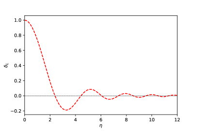
Figure 1: From top to bottom: linear density contrast $\hat{\delta}_{L}$ from Eq.(79), linear velocity perturbation $\hat{u}_{L}$ and linear mass perturbation $\delta\hat{M}_{L}$, for $\hat{\delta}_{L}(0)=1$.

IV.4.3 Numerical results

We show in Fig. 1 the linear density contrast, velocity and mass perturbations, normalized to $\hat{\delta}_{L}(0)=1$. In contrast with CDM self-similar solutions, which show a power-law falloff at large distance without oscillations, the fields oscillate around zero at the same frequency. In particular, we can see that these self-similar solutions correspond to compensated profiles, as the mass perturbation goes to zero at infinity and actually changes sign an infinite number of times. Positive density peaks approximately correspond to minima of the radial velocity perturbation and to zero-crossings of the mass perturbation. Of course, these oscillatory features are due to the quantum pressure (absent for CDM) which generates acoustic waves (but with a different dispersion relation than usual sound waves). We can see that the central density peak is much higher than the next peaks, which decrease as $1/\eta^{3}$ at large distance. This is due to the dimension three of space (i.e. the volume factor $\eta^{3}$) as the velocity and mass oscillations appear more regular.

As time grows, the profiles shrink in comoving coordinates as $x\propto t^{-1/6}$ from Eq.(62). The central peak becomes confined to an increasingly narrow region in comoving coordinates, with a decreasing mass. However, it is actually expanding in physical coordinates as $r\propto\sqrt{t}$.

In contrast with CDM solutions, the amplitude of the linear density-contrast profile does not evolve with time. However, the velocity and mass perturbations decay as $1/\sqrt{t}$, see the scaling laws (60).

IV.4.4 Balance of kinetic, gravitational and quantum-pressure terms

While the static solitons (33) are governed by the balance between gravity and the quantum pressure in (31), the self-similar solutions are dynamical and involve in addition kinetic effects, associated with the nonzero velocity, see (64). In fact, at large distance we obtain for $\eta\to\infty$

$$\hat{u}_{L}\sim\eta^{-5}+\eta^{-2}[\cos(\eta^{2})/6+\sin(\eta^{2})/6)],$$

$$\hat{\varphi}_{{\rm N}L}\sim\eta^{-4}+\eta^{-5}[\cos(\eta^{2})/6+\sin(\eta^{2})/6)],$$

$$\hat{\Phi}_{{\rm Q}L}\sim\eta^{-8}+\eta^{-1}[\cos(\eta^{2})/6+\sin(\eta^{2})/6)],$$ (85)

where we only wrote the leading smooth and oscillatory terms, omitting the numerical factors. Thus, we find that at large distance the Bernoulli equation (64) is governed by the balance between the kinetic energy and the quantum pressure, while gravity becomes negligible. This is possible thanks to the oscillations of the perturbed mass $\delta\hat{M}$ around zero, somewhat like a compensated density profile. This entails a screening of the central density peak and of its gravitational attraction, which makes gravity negligible at large radius. This is not totally surprising. Gravity is a long-range force, as shown by the inverse Laplacian in the Poisson equation (20), whereas the quantum pressure is a short-range force, as shown by the Laplacian in Eq.(17). This implies that the quantum pressure cannot balance gravity at large distance. Therefore, either gravity is balanced by the kinetic energy (as for the Hubble flow in the Einstein-de Sitter background), or it is screened by the compensated density profile. In the latter case, the small residual gravity can be balanced by the quantum pressure, but in our solution (85) the screening is so efficient that at large distance we simply have free waves, with a balance between the quantum pressure and kinetic terms, on top of the cosmological background. Of course, at the center where the velocity vanishes by symmetry we have instead a balance between gravity and the quantum pressure. Therefore, we have a change of the nature of the dynamics with the radius. It is set by gravity vs quantum pressure at the center and by kinetic terms vs quantum pressure at large distance.

IV.5 Comparison with CDM

Already at the linear level, we can see that the FDM self-similar solutions are very different from the CDM ones. First, the CDM linear modes $D_{\pm}(t)$ are scale-independent with $D_{+}(t)\propto t^{2/3}$ and $D_{-}(t)\propto t^{-1}$. We recover these power laws in the small-$\epsilon$ limit of Eq.(75). Since for CDM the space and time dependences factorize in Eq.(76), requirements on the shape of the density profile at an initial time do not rule out the growing nor the decaying mode. Then, one usually only keeps the growing mode, assuming that the decaying mode has had time to become negligible. In contrast, in Eq.(78) we only kept the mode $D_{-}$ because of the requirement to converge to the cosmological background on large scales. However, as we noticed below Eq.(78), for FDM the linear modes $D_{\pm}$ are no longer growing and decaying modes but acoustic oscillations of similar amplitude. Therefore, the self-similar solution associated with the mode $D_{-}$ is physical, as a small perturbation associated with the mode $D_{+}$ will remain small as long as we remain in the FDM regime where the quantum pressure is important. As seen in Eq.(85), this is valid at large radii in the linear regime. In fact, as seen in the lower panels in Figs. 2 and 3 below, this is valid at all radii at the nonlinear level for the self-similar solutions studied in this paper.

As the Newtonian equations of motion (50)-(52) only apply to sub-Hubble scales, one may consider introducing a large-scale cutoff at the Hubble radius, so that the FDM mode $D_{+}(k,t)$ does not lead to divergent quantities. Then, one may wonder whether one could recover the CDM self-similar solutions by first taking the semiclassical limit $\epsilon\to 0$ and next $c/H_{0}\to\infty$. This is better discussed in real space, as we detail below.

First, let us recall the main properties of the CDM self-similar solutions for the Einstein-de Sitter cosmology (Fillmore and Goldreich, 1984), associated with overdensities and the formation of spherical virialized halos. For an initial overdense power-law profile

$$0<\gamma<3:\;\;\;\delta_{L}(r)\propto r^{-\gamma}$$ (86)

of the linear density contrast, one obtains nonlinear self-similar solutions, with a turnaround radius that grows with time as

$$r_{\rm ta}(t)\propto t^{2/3+2/(3\gamma)}$$ (87)

and a nonlinear density profile in the inner virialized regions, for $r\ll r_{\rm ta}$, that shows a different power law,

$$\gamma\leq 2:\;\;\rho\propto r^{-2},\;\;\;\gamma\geq 2:\;\ \rho\propto r^{-3\gamma/(1+\gamma)}.$$ (88)

For shallow initial profiles, $\gamma<2$, the mass within a small radius $R$ is dominated by the particles that have just collapsed, whereas for steep initial profiles, $\gamma>2$, the mass within $R$ is dominated by the particles that have collapsed long ago, when the turnaround radius was of the order of $R$ (Fillmore and Goldreich, 1984). These solutions, which exhibit gravitational instability and collapse of increasingly massive and distant shells, originate from the growing mode $D_{+}(t)$ in the linear regime, with the power-law radial profile (86).

For FDM, the mode $D_{+}$ in (76) would correspond to a $k^{-7}$ profile in the semiclassical limit, which we discarded because of the low-$k$ divergence. By power counting, this corresponds to an $x^{4}$ profile in real space. This is indeed recovered in the real-space analysis of Sec. IV.4.2, in the linear mode $\delta_{L1}$ of Eq.(81), which grows as $\eta^{4}$ at large $\eta$ [from Eq.(62) we can check that the semiclassical limit $\epsilon\to 0$ corresponds to $\eta\to\infty$]. Comparing with Eq.(86), this corresponds at the formal level to $\gamma=-4$ and Eq.(87) gives for the characteristic scale at time $t$ the power law $r_{\rm ta}\propto\sqrt{t}$. Thus, we recover the square-root growth in physical coordinates obtained in Eq.(62).

Thus, for CDM the self-similar exponents, such as the growth of the characteristic scale in Eq.(87), span a continuous range, indexed on the slope $\gamma$ of the initial profile of the density contrast. In FDM, in addition to gravity we have the new quantum pressure in the hydrodynamical equations of motion. As can be expected, this new term restricts the possibility of self-similar solutions. Because it takes a power-law form, it still permits the existence of self-similar solutions but with a unique exponent, associated with the square-root growth of the physical scale in Eq.(62). As such, it selects among the CDM solutions (86)-(88) the one obtained for $\gamma=-4$, as this is the only exponent compatible with the quantum pressure term. However, this only holds at a formal level, because this value of the exponent $\gamma$ is beyond the allowed range in Eq.(86). In this sense, the semiclassical limit would make this FDM self-similar solution converge to a specific CDM self-similar solution (the one with the same exponent $\gamma$), but this is not possible or relevant in practice, because this specific solution is actually badly behaved (for both CDM and FDM) because it does not converge to the background on large scales.

Therefore, the allowed FDM self-similar solution, which we study in more details in this paper, does not correspond to a standard CDM self-similar solution. In fact, it would correspond to a different CDM self-similar solution associated with a decaying mode. For CDM, such a solution is not of great practical interest, as one expects to be dominated by growing modes. In contrast, as we noticed above, for FDM the linear modes $D_{\pm}$ are no longer growing and decaying modes but acoustic oscillations of similar amplitude. Therefore, the self-similar solution associated with the mode $D_{-}$ is physical, as a small perturbation associated with the mode $D_{+}$ remains small. In fact, we shall see in Sec. IV.6 that nonlinearities remain important at all scales, in the sense that the self-similar solution does not converge to the linear-theory prediction (84) at large radii, because it includes additional contributions associated with the modes $\delta_{L2}$ and $\delta_{L3}$.

Even though it does not have a standard CDM counterpart, it is still interesting to study this FDM self-similar solution for its own sake. It permits an analytical or semi-analytical treatment beyond static solitons and it provides an explicit example of gravitational cooling. Thus, it can help understand the dynamics generated by the competition between the quantum pressure, gravity and kinetic effects.

IV.6 Nonlinear regime

IV.6.1 Closed equation over $\delta M$

We now turn to the nonlinear regime and look for exact self-similar solutions of the equations of motion (50)-(52) of the form (60). In terms of the self-similar coordinate $\eta$, the Poisson equation reads

$$\frac{1}{\eta^{2}}\frac{d}{d\eta}\left(\eta^{2}\frac{d\hat{\varphi}_{\rm N}}{d\eta}\right)=\frac{2}{3}\hat{\delta},$$ (89)

while the quantum pressure reads

$$\hat{\Phi}_{\rm Q}=-\frac{1}{2\eta^{2}\sqrt{1+\hat{\delta}}}\frac{d}{d\eta}\left(\eta^{2}\frac{d}{d\eta}\sqrt{1+\hat{\delta}}\right).$$ (90)

The density contrast is given by the first derivative of the mass perturbation,

$$\hat{\delta}=\frac{3}{2\eta^{2}}\delta\hat{M}^{\prime}.$$ (91)

Integrating the continuity equation once over the radial coordinate gives the expression of the radial velocity in terms of the perturbed mass as

$$\hat{u}=\frac{3\delta\hat{M}-\eta\delta\hat{M}^{\prime}}{4\eta^{2}+6\delta\hat{M}^{\prime}}.$$ (92)

Substituting these expressions into the Euler equation (63), we obtain a closed nonlinear equation for the perturbed mass $\delta\hat{M}$,

$$9(2\eta^{3}+3\eta\delta\hat{M}^{\prime})^{2}\delta\hat{M}^{(4)}-(144\eta^{5}+216\eta^{3}\delta\hat{M}^{\prime}+108\eta^{4}\delta\hat{M}^{\prime\prime}$$

$$+162\eta^{2}\delta\hat{M}^{\prime}\delta\hat{M}^{\prime\prime})\delta\hat{M}^{(3)}+(4\eta^{8}+288\eta^{4}+36\eta^{5}\delta\hat{M}$$

$$-216\eta^{2}\delta\hat{M}^{\prime}+324\eta^{3}\delta\hat{M}^{\prime\prime}+81\eta^{2}\delta\hat{M}^{2}+81\eta^{2}\delta\hat{M}^{\prime\prime 2})\delta\hat{M}^{\prime\prime}$$

$$-3(4\eta^{7}+96\eta^{3}+180\eta^{4}\delta\hat{M}+243\eta^{2}\delta\hat{M}\delta\hat{M}^{\prime}-3\eta^{3}\delta\hat{M}^{\prime 2}$$

$$+108\delta\hat{M}\delta\hat{M}^{\prime 2})\delta\hat{M}^{\prime}-12\eta^{3}(7\eta^{3}-9\delta\hat{M})\delta\hat{M}=0.$$ (93)

IV.6.2 Comparison with the linear equation

If we linearize Eq.(93) we obtain the fourth-order linear equation

$$\mbox{(L1)}: 9\eta^{3}\delta\hat{M}^{(4)}-36\eta^{2}\delta\hat{M}^{(3)}+(72\eta+\eta^{5})\delta\hat{M}^{\prime\prime}$$ (94)

$$-3(24+\eta^{4})\delta\hat{M}^{\prime}-21\eta^{3}\delta\hat{M}=0,$$

whereas from the linear equation (80), using (91) we obtain the fifth-order linear equation

$$\mbox{(L2)}: 9\eta^{4}\delta\hat{M}_{L}^{(5)}-36\eta^{3}\delta\hat{M}_{L}^{(4)}+(108\eta^{2}+\eta^{6})\delta\hat{M}_{L}^{(3)}$$ (95)

$$-(216\eta+\eta^{5})\delta\hat{M}_{L}^{\prime\prime}+24(9-\eta^{4})\delta\hat{M}_{L}^{\prime}=0.$$

As it should, we can check that these two equations are related,

$$\mbox{(L2)}=\eta^{4}\frac{d}{d\eta}\left[\eta^{-3}\mbox{(L1)}\right].$$ (96)

Thus, the solutions of (L1) are also solutions of (L2). The latter being of order five instead of four, it includes the additional solution $\mbox{(L1)}\propto\eta^{3}$, corresponding to $\delta M_{L}={\rm constant}$, and hence to $\delta_{L}=0$. Therefore, the linearized equation (94) is fully consistent with the linear theory studied in Sec. IV.4.

IV.6.3 Numerical procedure

We solve the nonlinear equation (93) with a shooting method (Press et al., 1992), subdividing the spatial domain $\eta\geq 0$ in three regions: a central region $\eta\lesssim 0.1$, an intermediate region $0.1\lesssim\eta\lesssim 10$, and a large-distance region $\eta\gtrsim 10$. This allows for a convenient implementation of the boundary conditions.

We look for solutions that converge to the cosmological background at large distance, so that the density contrast and the perturbed mass go to zero. Therefore, at large distances we can use the linearized equation (94). This gives the four independent linear modes,

$$\begin{split}&\delta\hat{M}_{L1}=\eta^{3}\left(105+\eta^{4}\right),\\ &\delta\hat{M}_{L2}=\,_{2}F_{3}\left(-\frac{7}{4},\frac{3}{4};-\frac{1}{4},\frac{1}{4},\frac{1}{2};-\frac{\eta^{4}}{144}\right)+\frac{\sqrt{\pi}}{180\sqrt{3}}\delta\hat{M}_{L1},\\ &\delta\hat{M}_{L3}=\eta^{2}\,_{2}F_{3}\left(-\frac{5}{4},\frac{5}{4};\frac{1}{4},\frac{3}{4},\frac{3}{2};-\frac{\eta^{4}}{144}\right)-\frac{\sqrt{\pi}}{126\sqrt{3}}\delta\hat{M}_{L1},\\ &\delta\hat{M}_{L4}=\eta^{5}\,_{2}F_{3}\left(-\frac{1}{2},2;\frac{3}{2},\frac{7}{4},\frac{9}{4};-\frac{\eta^{4}}{144}\right)-\frac{\pi}{56}\delta\hat{M}_{L1}.\end{split}$$ (97)

Therefore, at large distance the perturbed mass is a combination of these four modes,

$$\eta\to\infty:\;\;\delta\hat{M}=\sum_{i=1}^{4}c_{i}\,\delta\hat{M}_{Li},$$ (98)

whith coefficients $c_{i}$ to be determined. For $\eta\to\infty$ the linear modes show the large-distance behaviors

$$\delta\hat{M}_{L2}=\cos(\eta^{2}/6)\left[\frac{2079}{\eta^{4}}+\dots\right]-\sin(\eta^{2}/6)\left[\frac{63}{\eta^{2}}+\dots\right],$$

$$\delta\hat{M}_{L3}=-\cos(\eta^{2}/6)\left[\frac{90}{\eta^{2}}+\dots\right]-\sin(\eta^{2}/6)\left[\frac{2970}{\eta^{4}}+\dots\right],$$

$$\delta\hat{M}_{L4}=-\cos(\eta^{2}/6)\left[\frac{405\sqrt{3\pi}}{2\eta^{2}}+\dots\right]$$

$$\hskip 22.76228pt+\sin(\eta^{2}/6)\left[\frac{405\sqrt{3\pi}}{2\eta^{2}}+\dots\right].$$ (99)

Therefore, we can see that the three modes $\delta\hat{M}_{L2}$, $\delta\hat{M}_{L3}$ and $\delta\hat{M}_{L4}$ obey the boundary condition $\delta\hat{M}\to 0$, while the divergent contribution from the mode $\delta\hat{M}_{L1}$ is ruled out. This gives the large-distance boundary condition

$$c_{1}=0.$$ (100)

To implement the boundary condition at the center, we write the Taylor expansion

$$\eta\to 0:\;\;\;\delta\hat{M}=a_{3}\eta^{3}+a_{5}\eta^{5}+a_{7}\eta^{7}+\dots,$$ (101)

corresponding to a density contrast with is finite and smooth at the center, with an expansion in even powers of $x$. In particular, the density contrast at the origin is

$$\hat{\delta}(0)=9a_{3}/2.$$ (102)

Thus, the central density contrast $\hat{\delta}(0)$ specifies the value of $a_{3}$. Next, substituting the expansion (101) into the differential equation (93) gives a hierarchy of equations that determines all higher-order coefficients $\{a_{7},a_{9},...\}$ in terms of $\{a_{3},a_{5}\}$. Thus, we are left with only one free parameter $a_{5}$, which is set by the boundary condition (100) at infinity.

In practice, we first choose the value of $\hat{\delta}(0)$, hence of $a_{3}$, of the profile we aim to compute. Then, for a trial value of $a_{5}$, we compute the profile $\delta\hat{M}(\eta)$ up to $\eta_{-}\sim 0.1$ with the Taylor expansion (101), all higher-order coefficients being known from the substitution into the differential equation (93). Next, we advance up to $\eta_{+}\sim 10$ by solving the nonlinear differential equation (93) with a Runge-Kutta algorithm. Then, at $\eta_{+}$, far enough in the linear regime, we match to the linear expansion (98). For a random initial guess $a_{5}$ at the center, this will give a nonzero coefficient $c_{1}$. Therefore, we use an iterative scheme over $a_{5}$ until the matching coefficient $c_{1}$ at the outer boundary $\eta_{+}$ vanishes. This sets the value of $a_{5}$.

In general, all three coefficients $c_{2},c_{3}$ and $c_{4}$ in the linear expansion (98) are nonzero. In contrast, the linear-theory solution (84) actually corresponds to the linear mode $\delta\hat{M}_{L4}$ only, with $c_{2}=c_{3}=0$. This corresponds to the fact that the linear modes $\delta\hat{M}_{L2}$ and $\delta\hat{M}_{L3}$ do not satisfy the appropriate boundary conditions at the center, $\eta\to 0$, which only leaves $\delta\hat{M}_{L4}$ as the unique solution (up to a normalization) for a linear solution valid over the full range $0\leq\eta<\infty$. This agrees with the fact that we obtained only one linear solution in Sec. IV.4.

Once we consider the exact nonlinear differential equation (93), matters are different and the modes $\delta\hat{M}_{L2}$ and $\delta\hat{M}_{L3}$ show nonzero contributions at large distances. This is because at the center the perturbations do not asymptotically vanish (contrary to what happens at $\eta\to\infty$) but remain finite, so that nonlinear contributions cannot be fully neglected. This changes the mapping between the boundary conditions at the center and at infinity and the large-distance modes $\delta\hat{M}_{L2}$ and $\delta\hat{M}_{L3}$ are no longer excluded because the behavior at the center of the linear modes is no longer relevant, as this central region is beyond strict linear theory. However, for $\hat{\delta}(0)\to 0$ the contributions from the modes $\delta\hat{M}_{L2}$ and $\delta\hat{M}_{L3}$ become small as compared with that from $\delta\hat{M}_{L4}$, as the solution converges to the linear theory.

Therefore, in contrast with the CDM self-similar solutions, for a finite central density there is never convergence to the linear theory at large distance, in the sense that $\delta\hat{M}(\eta)$ does not converge to $\delta\hat{M}_{L}(\eta)\propto\delta\hat{M}_{L4}(\eta)$. Indeed, the additional modes $\delta\hat{M}_{L2}$ and $\delta\hat{M}_{L3}$ also decrease as $1/\eta^{2}$, with oscillatory prefactors. This is due to a strong coupling between the behaviors at the center and at infinity. This arises from the self-similarity of the solution and from the quantum pressure (absent for CDM) which propagates information from the center to infinity and vice versa (by looking for a self-similar solution we have implicitly provided an infinite amount of time to acoustic waves to propagate over all space). Physically, the blow-up character of the solutions means that the scalar matter starts in the nonlinear regime at small radii, and ends in the linear regime (i.e. converges to the Hubble flow) at late times and large radii, as explicitly seen in Sec. IV.10. This is the opposite of the usual CDM collapsing solutions, where matter shells start in the linear regime and finally collapse and virialize in the nonlinear inner regions. This couples the final linear era to the initial nonlinear era.

IV.7 Overdensities

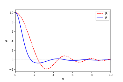
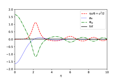
Figure 2: Upper panel: nonlinear density contrast $\hat{\delta}$ (blue solid line) and linear density contrast $\hat{\delta}_{L}$ (red dashed line), for $\hat{\delta}(0)=10$. Middle panel: nonlinear and linear velocity fields. Lower panel: comparison of the terms in the Bernoulli equation (64). We show the kinetic part (red dashed line), the Newtonian gravitational potential (blue dotted line), the quantum pressure (green dot-dashed line), and their sum which must be zero (black solid line).

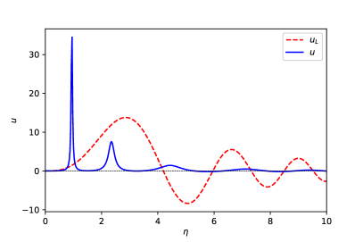
Figure 3: Nonlinear and linear solutions as in Fig. 2, but for $\hat{\delta}(0)=100$.

We compare in Figs. 2 and 3 the nonlinear and linear densities and the velocity perturbations, for the cases $\hat{\delta}(0)=10$ and $100$. We can see that as the height of the central density peak grows, the nonlinear corrections make the peak narrower and all the higher-order peaks move closer to the center. The oscillations of the velocity field also grow and become much sharper. They are no longer symmetric and the velocity shows high and narrow positive spikes at the density minima, where $\hat{\delta}\simeq-1$ and $\rho\simeq 0$. This can be understood from the scalar matter flux. As we have explained in Sec. IV.4.3, the profile shrinks in comoving coordinates and loses mass as time grows. Then, for the scalar mass to escape from the central peak across the radius $R_{1}(t)$, associated with the first minimum of the density, the velocity must be large to ensure a large flux despite the small local density. This also holds for the next few peaks where the density minima are also much below the background density.

This ejection of scalar matter, through successive clumps that escape from the central density peak and move to infinity, is also seen in numerical simulations and often called “gravitational cooling” (Seidel and Suen, 1994; Guzman and Urena‐Lopez, 2006). This allows the system to relax towards equilibrium configurations, in spite of the absence of dissipative processes, by ejecting extra matter and energy to infinity. Of course, in simulations that follow for instance the collisions of DM halos, this transient process is somewhat chaotic, whereas in our self-similar solutions it is well ordered and takes place at all times, up to a rescaling of length and mass scales. However, it is interesting to recover this process in the simple and semi-analytic self-similar solutions studied in this paper. We shall come back to this ejection of matter in Sec. IV.10 below, where we compute the trajectories of constant-mass shells.

As explained in Sec. IV.4.3 from the linear solution, these dynamics involve a changing interplay between gravity, quantum pressure and kinetic effects. This phenomenon remains valid in the nonlinear regime, as seen in the lower panels that show the various terms in the Bernoulli equation (64). Near the center, gravity and the quantum pressure play the major roles, as the velocity vanishes at the center by symmetry. Gravity ensures that the central overdensity does not decay too fast and actually follows the cosmological background density, whereas the quantum pressure resists the gravitational pull and ejects some matter outside of the central peak. As the central density becomes very large (see Fig. 3), this dominance of gravity and quantum pressure extends over several density peaks, with sharp transitions at the density minima associated with the spikes of the velocity field, and hence of the kinetic terms, balanced by spikes of the quantum pressure. Indeed, being an integral of the matter density, the gravitational potential $\varphi_{\rm N}$ is very smooth and cannot follow the sharp changes of the velocity. In contrast, the quantum pressure (53) being the second derivative of the density, it is a local quantity that responds to local changes of the system. At larger distances, where we recover the linear regime, the gravitational potential becomes negligible as the mass perturbation is screened, like for a compensated profile. There, the quantum pressure and kinetic terms play the dominant roles and scalar fluctuations travel afar in a wavelike fashion. Thus, we can see how the gravitational cooling is related to the wavelike features of the FDM dynamics, thanks the relevance of the quantum pressure.

The numerical computation shows that the density contrast always remains above $-1$, and hence the density never vanishes and remains strictly positive. This can be shown analytically as follows. Let us look for a regular solution with a vanishing density at the point $\eta_{0}$,

$$\delta\hat{M}(\eta)=a_{0}+a_{1}(\eta-\eta_{0})+a_{2}(\eta-\eta_{0})^{2}+\dots,$$ (103)

with the zero-density constraint

$$\hat{\delta}(\eta_{0})=-1:\;\;\;a_{1}=-\frac{2}{3}\eta_{0}^{2}.$$ (104)

Substituting into the equation of motion (93) determines the coefficients $a_{2},a_{3},....$, and gives the solution

$$\delta\hat{M}(\eta)=a_{0}-\frac{2}{9}(\eta^{3}-\eta_{0}^{3}),$$ (105)

where $a_{0}$ remains undetermined. We can check that this is indeed a solution of Eq.(93) and it yields $\hat{\delta}(\eta)=-1$, that is, the constant zero-density solution $\rho=0$. Thus, the only regular self-similar solution where the density vanishes at a point is actually the homogeneous vacuum. This implies that the nonlinear density profiles shown in Figs. 2 and 3 can never touch the zero-density threshold. The fact that the density always remains strictly positive means that the Madelung transformation (14) is always well defined and the $\psi$-field and $\{\rho,\vec{v}\}$-hydrodynamical pictures are equivalent. Therefore, the self-similar solutions obtained from (93) in terms of $\{\rho,\vec{v}\}$ give at once the self-similar solutions in terms of $\psi$ and we do not miss any by working in the hydrodynamical framework. In fact, because our solutions are spherically symmetric the spatial dimensionnality is reduced to one and the radial velocity can always be written as the gradient of a phase $S=\int dr\,v_{r}$, so that the Schrödinger and hydrodynamical pictures are equivalent.

IV.8 Underdensities

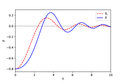
Figure 4: Nonlinear and linear solutions as in Fig. 2, but for $\hat{\delta}(0)=-0.8$.

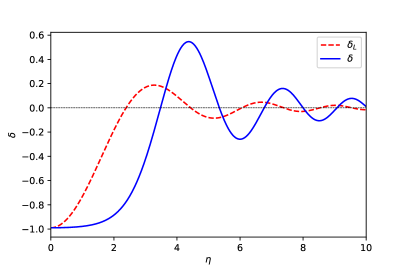
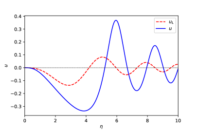
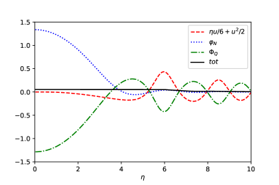
Figure 5: Nonlinear and linear solutions as in Fig. 2, but for $\hat{\delta}(0)=-0.99$.

We show in Figs. 4 and 5 the case of underdense central regions, $\hat{\delta}(0)=-0.8$ and $-0.99$. As compared with the linear profiles, we find that nonlinear corrections now move the density peaks to larger distance and widen the central void, in contrast with the overdense case. Again, by symmetry the velocity vanishes at the center so that the gravitational and quantum pressure terms dominate in the Bernoulli equation (64), while the kinetic and quantum pressure terms dominate at large distance in the linear regime, where the mass perturbation is screened as for a compensated profile.

Again, the density contrast always remains above $-1$, that is, the density $\rho$ is always strictly positive, and the equivalence of the $\psi$-field and $\{\rho,\vec{v}\}$-hydrodynamical pictures is valid.

IV.9 Husimi distribution

IV.9.1 Overdensities

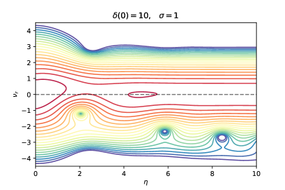
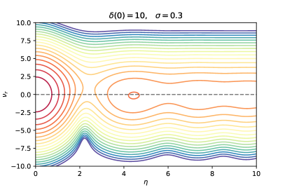
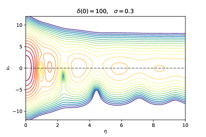
Figure 6: Isodensity contours for the radial Husimi distribution function $\hat{f}_{\rm H}(\eta,\nu_{r})$ for $\sigma=1$ (upper row, $\delta(0)=10$ and $100$) and for $\sigma=0.3$ (lower row, $\delta(0)=10$ and $100$).

We show in Figs. 6 the radial Husimi distributions $\hat{f}_{\rm H}(\eta,\nu_{r})$, where $\nu_{r}$ is the radial velocity. As seen in Figs. 2 and 3, as the central density increases successive density peaks are more clearly defined and separated by almost void regions. This is also seen in the Husimi distribution, with the number of well-defined peaks increasing with $\delta(0)$. At large distance, where the profile converges to the cosmological background, the finite smoothing $\sigma$ involved in the definition of the Husimi distribution smears out the density and velocity perturbations and the Husimi distribution converges to the background result (72).

As the spatial coarsening $\sigma_{x}\propto\sigma$ decreases, the velocity coarsening $\sigma_{p}\propto 1/\sigma$ increases, following the Heisenberg uncertainty principle (69). Thus, for the case $\delta(0)=10$ with $\sigma=1$, we can see the velocity asymmetry inside the central peak (the radial velocity is positive as seen in Fig. 2) but the spatial profile is somewhat smoothed out. Decreasing $\sigma$ to $0.3$ gives a better separation between the first two peaks and preserves signs of the density fluctuations at larger radii, but this comes at the price of a significant smoothing along the velocity axis and the asymmetry of the velocity distribution in the central peak can no longer be distinguished. Note that the scale of the vertical velocity axis is larger for the lower panels with $\sigma=0.3$. In fact, in the limit $\sigma\to 0$ we have $\hat{f}_{\rm H}\sim\sigma^{3}\pi^{-3/2}\hat{\rho}(\eta)$ at fixed $\vec{\nu}$.

For $\delta(0)=100$ the spatial width of the central and few subsequent peaks shrinks, as seen in Fig. 3. This implies that the coarsening $\sigma=1$ is no longer sufficient to separate the first few peaks. This leads to artificial interferences between these peaks and to a Husimi distribution that is difficult to interpret and far from the semiclassical expectations. Decreasing $\sigma$ to $0.3$ gives a more faithful representation of the system, as we can clearly see the sequence of scalar-field clumps. However, this erases most of the information about the velocity field.

This shows that it is not always straightforward to use the Schrödinger equation (54) and the Husimi distribution as an alternative to N-body simulations to compute the classical phase-space distribution that obeys the Vlasov equation. Different choices of the smoothing $\sigma$ can lead to rather different pictures that can be difficult to relate to the underlying dynamics. This may become a problem for systems that exhibit a large range of scales, as for the hierarchical gravitational clustering displayed by cosmological structures. For the self-similar solutions that we study in this paper, where the density is everywhere strictly positive and the hydrodynamical mapping (14) well defined, the density and velocity fields provide a clearer picture of the dynamics than the phase-space Husimi distribution.

IV.9.2 Underdensities

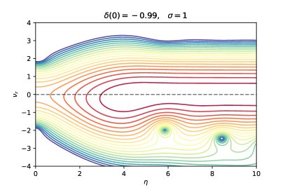
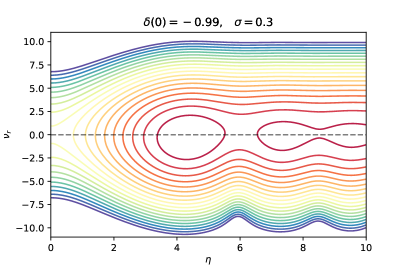
Figure 7: Isodensity contours for the radial Husimi distribution function $\hat{f}_{\rm H}(\eta,\nu_{r})$, for $\sigma=1$ (upper panel) and $\sigma=0.3$ (lower panel) with $\delta(0)=-0.99$.

We show in Fig. 7 the case of the central underdensity $\delta(0)=-0.99$. Again, we find that the smaller value of $\sigma$ enables a better separation of the successive density peaks but erases the velocity asymmetries.

IV.10 Trajectories associated to the self-similar solutions

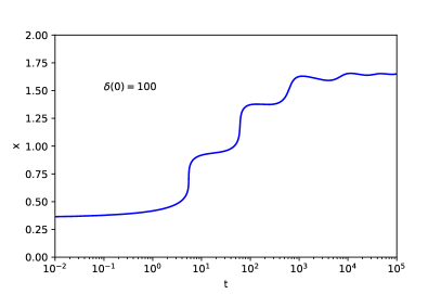
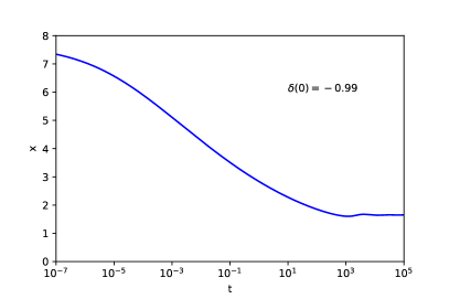
Figure 8: Trajectory $x(t)$ of the comoving radius associated with a fixed mass, as a function of cosmic time $t$. We show the case of the self-similar solutions defined by the central density contrasts $\delta(0)=100$ (upper panel) and $\delta(0)=-0.99$ (lower panel).

The density and velocity fields, as well as the Husimi distribution, provide an Eulerian point of view on the self-similar solutions. To understand better the dynamics it is useful to consider a complementary Lagrangian point of view. Thanks to the spherical symmetry, in the hydrodynamical picture the analogue of a particle trajectory is the motion of the radius $r(t)$ that encloses a fixed mass $M(<r)=M$. From Eq.(60), the mass $M(<r)=\bar{M}+\delta M$ reads

$$M=\bar{M}+\delta M=\epsilon^{3/2}t^{-1/2}\left[\frac{2}{9}\eta^{3}+\delta\hat{M}(\eta)\right].$$ (106)

This implicitly gives the trajectory $\eta(t)$ as a function of time for a given mass. In fact, from Eq.(106) we obtain at once the scaling law

$$\eta(t|M,\epsilon)=\eta(\epsilon^{-3}M^{2}t),$$ (107)

that is, $\eta$ only depends on the combination $\epsilon^{-3}M^{2}t$. Therefore, trajectories associated with different masses or different values of $\epsilon$ can be obtained from a single trajectory by a rescaling of time,

$$t\propto\epsilon^{3}M^{-2}.$$ (108)

However, the shape of the trajectory depends on the self-similar profile, defined for instance by the central density contrast $\delta(0)$. The result (108) shows that large masses correspond to small times, in contrast with the self-similar CDM solutions that describe a hierarchical collapse where large masses collapse later Fillmore and Goldreich (1984); Bertschinger (1985). This is because the FDM self-similar solutions describe instead a slow blow-up, that roughly follows the Hubble expansion. Indeed, as the total overdensity $1+\delta$ is always positive, at fixed time $M(\eta)$ and $\eta(M)$ are monotonic increasing functions. The scaling law (107) then implies that $\eta(t)$ is also a monotonic increasing function of $t$ at fixed $M$. Therefore, at $t\to 0$ we have $\eta\to 0$ and at $t\to\infty$ we have $\eta\to\infty$. Thus, in terms of the rescaled radius $\eta$, at early time the mass shell starts close to origin, inside the central peak or void, far in the nonlinear regime if the self-similar solution is nonlinear at the center, whereas at late time the mass shell moves increasingly far in the linear regime, at large distance. Thus, whereas the trajectories found in the CDM self-similar solutions describe a spherical collapse that runs from the linear to the nonlinear regime, the trajectories found in the FDM self-similar solutions describe an expansion that runs from the nonlinear to the linear regime, independently of whether the central region is overdense or underdense.

We show in Fig. 8 the trajectories obtained inside the self-similar solutions defined by $\delta(0)=100$ and $-0.99$. We plot the trajectories $x(t)$ in terms of the comoving coordinate, using Eq.(62), which gives $x(t)=\epsilon^{1/2}t^{-1/6}\eta(t)$. For the numerical computations we take $\epsilon=1$, $M=1$; as explained in Eq.(108) other values of $\epsilon$ or $M$ only correspond to a rescaling of time and radius. We can see that in all cases the trajectories roughly follow the Hubble expansion, as the comoving radius $x(t)$ goes to nonzero finite values at both small and large times. This agrees with the scaling $\delta=\hat{\delta}(\eta)$ in (60), which means that the typical density $\rho$ follows the decrease of the background density $\bar{\rho}\propto t^{-2}$. Indeed, this clearly implies that mass shells cannot expand much more slowly or faster than the Hubble flow. At late times, which correspond to large $\eta$, the background term $2\eta^{3}/9$ dominates in the bracket in Eq.(106). This means that, independently of $\delta(0)$, we recover the Hubble flow with $x(t)\simeq\bar{x}$, where $\bar{x}=(9/2)^{1/3}M^{1/3}$ is the background comoving radius associated with the mass $M$. On top of this asymptotic value we have subdominant oscillations associated with the linear regime. This also corresponds to the limit of large masses, as they are at larger radii further into the linear regime.

For the overdense case, we can see that the comoving radius $x(t)$ increases from its initial to its final value. This is because the mass shell is initially inside the central density peak, close to the origin. This overdense configuration implies an initial radius $x_{i}$ that is smaller than its counterpart $\bar{x}$ in the background universe, for the same mass $M$ (as $\rho\propto M/x^{3}$). At late time, as we recover the Hubble flow with increasingly small perturbations, the trajectory converges to $\bar{x}>x_{i}$. Conversely, for the underdense case, the comoving radius $x(t)$ decreases from its initial to its final value. In the case of the high central overdensity $\delta(0)=100$, where there are three well marked density peaks separated by velocity spikes, see Fig. 3, the trajectory has an intermittent character with well-distinguishable steps in the nonlinear regime. The comoving radius grows very slowly when the shell is inside the density peaks, or clumps, and shows fast accelerations as it moves from one clump to the next, because of the velocity spikes found in Fig. 3, associated with the voids that separate the clumps. For the underdense case $\delta(0)=-0.99$ the secondary peaks and their velocity spikes are weak, see Fig. 5, and we cannot distinguish well-marked steps in the trajectory.

Although the self-similar profile shrinks in comoving coordinates, as $x\propto t^{-1/6}$ at fixed $\eta$ from Eq.(62), the mass-shell trajectories remain roughly constant, with a global finite increase for overdense cases and a global finite decrease for underdense cases. Thus, as for wave packets where one needs to distinguish the group and phase velocities, we can distinguish two velocities or trajectories in the self-similar solutions. We have a “geometric” trajectory, $x\propto t^{-1/6}$, that describes the shrinking of the self-similar profile, and a “matter” trajectory, $x\sim{\rm constant}$, that describes the flow of matter. They correspond to $r\propto t^{1/2}$ and $r\sim t^{2/3}$ in physical coordinates. In particular, as explained above, matter flows “through” the self-similar profile towards the large-distance linear regime. It escapes from the nonlinear central region, going through a series of clumps and velocity bursts, until it converges to the Hubble flow at large distance. This ejection of matter is reminiscent of the gravitational cooling found in numerical simulations.

Therefore, the matter content of a given clump does not remain fixed with time, as matter slowly flows through it (and reaches large velocities at its boundaries, where the density is very small). Again, this is reminiscent of the behaviors of system governed by wave equations. Here this is due to the quantum pressure, which originates from the Schrödinger equation that exhibits well-known wavelike and interference behaviors.

V High-density asymptotic limit

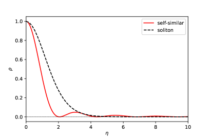
Figure 9: Asymptotic self-similar (red solid line) and soliton (black dashed line) density profiles, normalized to $\rho(0)=1$.

We recalled in Sec. II that the SP system (3)-(4) is invariant under the scaling law (5). In the case of the cosmological self-similar solutions, this symmetry is broken by the Einstein-de Sitter background that sets the boundary condition at large distance. In contrast with the family of solitonic solutions (33) in vacuum, we can no longer obtain a family of self-similar solutions by the rescaling (5), as this would also change the density at infinity (and hence correspond to a different boundary condition). However, in the limit of large density contrasts, the background density becomes negligible as compared with the central density and we can expect the inner profile to converge to a limiting shape that obeys the scaling law (5), which reads here

$$\left\{\eta,\psi,\rho,M\right\}\rightarrow\left\{\lambda^{-1}\eta,\lambda^{2}\psi,\lambda^{4}\rho,\lambda M\right\}.$$ (109)

We can obtain the equation satisfied by this limiting profile by substituting these scalings into Eq.(93) and keeping only the leading terms in the limit $\lambda\to\infty$. This gives

$$M^{\prime 2}M^{(4)}-2M^{\prime}M^{\prime\prime}M^{(3)}+M^{\prime\prime 3}=\frac{4}{\eta^{2}}MM^{\prime 3}\;.$$ (110)

In this limit we identified $M\simeq\delta\hat{M}$ and $\rho\simeq\hat{\delta}$, so that the density is given by $\rho=3M^{\prime}/(2\eta^{2})$. This nonlinear equation is then invariant under the symmetry (109). This means that a complete family of solutions can be obtained from one solution, normalized for instance by $\rho(0)=1$, by the rescaling (109). Solving Eq.(110) is actually more difficult than finding solutions of Eq.(93), as the density minima between the successive peaks now touch the vacuum value $\rho=0$. These points, where $M^{\prime}=M^{\prime\prime}=0$, are singular points of the differential equation (110). In practice, we compute the finite-$\lambda$ profile defined by Eq.(93) and check that for large $\delta(0)$ the curves collapse to a unique profile normalized to $\rho(0)=1$ after applying the scaling (109). We also checked that this profile approximately satisfies Eq.(110).

We compare in Fig. 9 this asymptotic self-similar profile with the soliton profile obtained from Eq.(33), which reads in terms of the dimensionless variables

$$\nabla^{2}_{\eta}\psi_{\rm sol}=2(\varphi_{\rm N}-\alpha)\psi_{\rm sol},\;\;\;\nabla^{2}_{\eta}\varphi_{\rm N}=\frac{2}{3}\psi_{\rm sol}^{2}.$$ (111)

We can see that the two profiles do not coincide. Thus, even as the central density increases the shape of the central peak of the self-similar profile does not converge to the soliton equilibrium. This is due to the importance of kinetic effects, which dominate near the boundary of the central peak as seen in the lower panel in Fig. 3. Besides, beyond the kinetic terms, the soliton balance equation (31) differs from the self-similar Bernoulli equation (64) by the $\alpha$ parameter on the right-hand side. Thus, the two profiles are different and the central peak of the self-similar solution is narrower than the soliton peak. Therefore, even though at large densities the local timescale inside the central peak becomes much smaller than the Hubble time, the profile does not relax towards the static soliton profile. This shows that the convergence towards the soliton core is not guaranteed in all configurations.

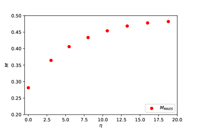
Figure 10: Mass of the density peaks for the asymptotic self-similar density profile normalized to $\rho(0)=1$

At large radius, we can neglect the right-hand side in Eq.(110). This gives a homogeneous equation that can be solved as

$$\eta\to\infty:\;\;\;\rho\simeq\frac{3b}{2\eta^{2}}\cos^{2}\left[\frac{a(\eta-\eta_{0})}{\sqrt{2}}\right],$$

$$M\simeq M_{0}+b\left[\frac{\eta-\eta_{0}}{2}+\frac{\sin[\sqrt{2}a(\eta-\eta_{0})]}{2\sqrt{2}a}\right],$$ (112)

where the parameters $M_{0},\eta_{0},a$ and $b$ are undetermined (one needs to solve the complete equation (110) to derive their value). We can check that the density is always positive but now vanishes on an almost periodic set of radii. Thus, the oscillations of the asymptotic profile have equal length in the radius $\eta$, while the linear-profile oscillations had equal lengths in $\eta^{2}$, as seen in Eq.(83). The nonlinear effects both move the density peaks towards the center and change their scaling with distance. The enveloppe of the density oscillations decreases like $1/\eta^{2}$, while the soliton density shows an exponential falloff. This also implies that the mass grows linearly with the radius, so that each peak (or more precisely each shell in the 3D space) contains the same mass. Thus, the outer shells are not as negligible as appears in the density plots. This is also shown in Fig. 10, where we plot the mass associated with the first few density peaks (i.e. the mass in each spherical shell delimited by minima of the density).

VI CDM comparison, semiclassical limit and conclusion

As we recalled in Eqs.(86)-(88), self-similar solutions for collisionless matter in a perturbed Einstein-de Sitter universe have been obtained by Fillmore and Goldreich (1984). Using a different method, these results were recovered and extended to collisional gas by Bertschinger (1985). These solutions describe the gravitational collapse of spherical overdense regions or the expansion of voids. Thus, starting at early times with a small linear perturbation $\delta_{L}(r,t_{i})$, which follows the power-law profile (86), the density contrast grows as $t^{2/3}$, according to the linear growing mode, until it reaches the nonlinear regime. Then, nonlinear effects modify the shape of the profile in the inner regions. At small radii it takes again a power-law form, as in Eq.(88), but with a different exponent that depends on the slope of the linear seed. Thus, one obtains a family of solutions, characterized by the slope $\gamma$ of the density perturbation at large distance. For the collisional case, the profile also depends on the adiabatic index $\gamma_{\rm ad}$. In the case of overdense regions, these self-similar solutions display a gravitational instability and increasingly distant shells collapse. They typically stabilize at a fixed fraction of their turnaround radius, as gravity is balanced either by the radial velocity dispersion or by the thermal pressure (in the collisional case). This leads to a virial equilibrium in the inner nonlinear core, with a mass and a radius that grow with time, both in physical and comoving coordinates.

The self-similar solutions we have obtained in this paper for FDM are very different. They do not follow power-law shapes and their amplitude does not grow with time. Thus, the density contrast at the center, $\delta(0)$, remains constant. This implies that the gravitational instability is balanced by the quantum pressure and there is no transition from the linear to the nonlinear regime for the profile as time increases. The profile remains linear on all scales and at all times or remains nonlinear in the center.

In contrast with the CDM case, the large-distance and linear-theory limits no longer coincide. Although at large radii the density perturbation becomes small and a linear treatment is valid, the profile does not converge to the linear-theory profile. This is because at large distance we have nonzero contributions from the three linear modes that are well behaved at infinity, while the linear theory selects only one of them, which satisfies in addition the boundary condition at the center.

The constant amplitude with time also means that these solutions do not exhibit a gravitational collapse. In fact, both for underdense and overdense central regions, the mass contained in the central peak or “void” decreases with time as $M\propto t^{-1/2}$. The associated radius increases as $t^{1/2}$ in physical coordinates but decreases as $t^{-1/6}$ in comoving coordinates. Thus, instead of accreting mass, the central region continuously expels matter. In the nonlinear regime, this occurs through well-separated clumps that travel outward in physical coordinates, in a fashion similar to the expulsion of matter in gravitational cooling. However, in these self-similar solutions matter does not remain trapped inside each clump and moves outward faster, leaking from one clump to the next one through a low-density but high-velocity narrow region. At large radii, in the linear regime, we have acoustic waves around the cosmological background as the central overdensity is screened as for a compensated profile, so that the gravitational force is negligible as compared with kinetic and quantum-pressure terms.

The characteristic exponents $M\propto t^{-1/2}$, $r\propto t^{1/2}$, are universal, in contrast with the continuous range of exponents obtained in the CDM case, which depend on the slope $\gamma$ of the linear seed. As explained in Sec. IV.5, this is due to the new force associated with the quantum pressure, in addition to gravity. This new term in the equations of motion is only compatible with the exponent $\gamma=-4$. However, this value is beyond the allowed range Eq. (86) for the standard CDM self-similar solutions. In fact, the self-similar FDM solutions studied in this paper are instead associated with a non-standard CDM solution, which would correspond to a decaying mode in the linear regime and as such is unphysical. However, the separation between growing and decaying modes disappears in the FDM regime, where the quantum pressure turns both modes into acoustic oscillations of constant amplitude. Thus, the FDM case shows strong qualitative differences with the CDM case. Because of self-similarity, these differences remain important in the solutions studied in this paper at all times and scales. They do not disappear either in the limit $\epsilon\to 0$ because $\epsilon$ is fully absorbed by the change to the self-similar coordinate $\eta$ in Eq.(62).

As explained above, the profile at large distance, although within the linear regime of small perturbations, differs from the linear-theory profile by two additional linear modes, with coefficients that depend on the central density. Thus, in contrast with the CDM case, we have a strong coupling from the small inner radii onto the large outer radii. Indeed, in the CDM non-collisional case Fillmore and Goldreich (1984); Bertschinger (1985), outer shells are decoupled and follow the spherical collapse, which only depends on the inner mass from Gauss theorem and not on the density profile. This means that they collapse as in free fall (with an initial outward velocity close to the Hubble flow) until shell crossing occurs at nonlinear radii (which implies the mass within each shell is no longer constant and the dynamics become more complex). Similarly, in the collisional collapse of a polytropic gas, the pressure at large radii beyond the shock (located around the virial radius) is zero (because one starts from cold initial conditions), so that free-fall spherical collapse also applies. The pressure becomes nonzero at the shock, associated with a jump of the temperature and of the entropy, and balances gravity at smaller radii Bertschinger (1985); Teyssier et al. (1997). In contrast, for the self-similar solutions of FDM, outer shells do not follow a spherical free fall. This is because the effective “pressure”, associated with the quantum pressure, is not zero. Instead, together with kinetic terms, it dominates over gravity. This leads to acoustic-like oscillations, or waves, that transport information from small to large scales and build this coupling between small and large scales.

As the Schrödinger equation (54) was also proposed (Widrow and Kaiser, 1993; Uhlemann et al., 2014; Mocz et al., 2018; Garny et al., 2020) as an alternative to N-body simulations to compute the evolution of CDM in the semiclassical limit, $\epsilon\to 0$, one can be surprised by this large difference between the self-similar solutions. Indeed, in the semiclassical limit one expects to recover the CDM dynamics. The point is that this is a weak limit that is not so straightforward. As shown by the scalings (60) and (62), what happens is that these FDM self-similar solutions “disappear” in the semiclassical limit, as their size and their mass decrease as $\epsilon^{1/2}$ and $\epsilon^{3/2}$ for $\epsilon\to 0$. Thus, in the semiclassical limit, they become confined to an increasingly small radius. This counterbalances the $\epsilon^{2}$ factor in front of the Laplacian in the Schrödinger equation (54), so that for any finite $\epsilon$ we have a self-similar solution where the quantum pressure remains able to balance gravity near the center. However, from a macroscopic point of view, this configuration becomes irrelevant as it becomes infinitesimal. The standard CDM self-similar solutions are only exactly recovered at $\epsilon=0$, or as approximate solutions at small $\epsilon$ with a small breaking of the self-similarity. In other words, the standard CDM self-similar solutions are not the limit at $\epsilon\to 0$ of the FDM self-similar solutions. This also shows that the semiclassical limit needs to be considered with care. If in the limit $\epsilon\to 0$ gradients become steep enough, they can sustain dynamics quite different from the CDM Vlasov case and the limit can become nontrivial.