Stability analysis of anisotropic Bianchi type-I cosmological model in teleparallel gravity

Abstract

Abstract:In this work, we study a cosmological model of Bianchi type-I Universe in teleparallel gravity for a perfect fluid. To obtain the cosmological solution of the model, we assume that the deceleration parameter is a linear function of the Hubble parameter $H$ i.e. $q=-1+\beta H$ (where $\beta$ as a positive constant). Consequently, we get a model of our Universe, where it goes from the initial phase of deceleration to the current phase of acceleration. We have discussed some physical and geometric properties such as Hubble parameter, deceleration parameter, energy density, pressure, and equation of state (EoS) parameter and study their behavior graphically in terms of redshift and compare it with observational data such as Type Ia supernovae (SNIa). We also discussed the behavior of other parameters such as the Jerk parameter, Statefinder parameters and we tested the validity of the model by studying the stability analysis and energy conditions.

Keywords: Bianchi type-I Universe, $f\left(T\right)$ gravity, Dark energy, Stability analysis, Observational data.

I Introduction

Since Einstein ref1 published his theory of General Relativity (GR) in 1916 until the end of the previous century, cosmologists believed that the Universe was in a decelerated phase of expansion, due to Friedmann’s equations in the standard model of cosmology ref2 . But recently, a group of theoretical and observational studies appeared in cosmology which showed the opposite, that is to say, that our current Universe is in a phase of accelerated expansion ref3 ; ref4 ; ref5 ; ref6 ; ref7 . This contradiction between theories and observational data has led many researchers to suggest other alternatives that agree between the two ref8 . The most famous is the idea that there is a new form of energy called dark energy (DE) which is causing the accelerating expansion of the Universe. According to the observational data, DE is characterized by negative pressure or in some other way a negative EoS parameter $\omega$, where $\omega=\frac{p}{\rho}$ with $\rho$ represents the energy density of the Universe and $p$ represents the pressure. Many researchers recommend another idea, namely that the accelerating expansion of the Universe could be the result of modifications of gravity, and they called this class the Modified Gravity Theories (MGT), see ref9 ; ref10 ; ref11 ; ref12 ; ref13 ; ref14 . Another class combines the holographic principle with DE, such as ref15 . Many researchers around the world are striving to uncover the causes of cosmic acceleration, but despite this, the question of cosmic acceleration or DE remains a mystery in the scientific arena. Another simple idea about the nature of DE in the context of GR was to add the cosmological constant $\Lambda$ that Einstein had introduced into his equations in another context, but soon many problems arose, for example, it was a difficulty on the theoretically predicted order of magnitude compared to that of the observed vacuum energy ref16 ; ref17 .

Recently, a new type of study has appeared, which attempts to explain the accelerated expansion of the Universe by assuming cosmological models in various gravitational theories that contain the deceleration parameter or in another way the scale factor which varies over time ref18 ; ref19 ; ref20 . Indeed, this hypothesis is supported by observational data which shows that the Universe has passed from the stage of early deceleration $(q>0)$ to the stage of current acceleration $(q<0)$.

Among all these modified gravity theories found in the literature, in this work, we will focus on another approach to examine alternatives to GR which is Teleparallel Gravity (TG) which uses the Weitzenbock connection in place of the Levi–Civita connection and therefore does not have curvature but has a torsion which is responsible for the acceleration of the Universe. Some studies on this subject have gone so far as to replace scalar torsion $T$ with a generalized function $f(T)$ for the latter ref21 . For example, Bhoyar et al. study Bianchi type-I space-time for the linear and quadratic form of $f(T)$ gravity with a hybrid expansion law for scale factor ref22 . Holographic DE has also been discussed in this context by Shaikh et al. using the power and exponential laws ref23 . In another work, Shaikh studies DE in a teleparallel gravity framework using the hybrid expansion law for scale factor with the thermodynamic aspects of the model ref24 . See also other works in this context ref25 ; ref26 ; ref27 ; ref28 ; ref29 .
Several studies support the idea that the geometry of the Universe at the end of the inflationary era is homogeneous and isotropic ref30 , so that FLRW models play an important role in this period. However, defects in the cosmic microwave background (CMB) due to quantum fluctuations of the inflation period confirm the existence of an anisotropic phase which then transformed into an isotropic phase. Recently, with the advent of Planck observational data ref31 , Bianchi cosmological models describing the anisotropic Universe have attracted the attention of many authors. In the literature, there are several types of anisotropic and inhomogeneous Bianchi space-times. The Bianchi type-I space-time is the mathematically simplest case that describes an anisotropic and homogeneous Universe. Also defined as a direct generalization of the FLRW Universe with a different scale factor in each spatial direction. Several Bianchi type-I cosmological models have been studied in various contexts by many researchers. Recently, Hossienkhani et al. studied the spatially homogeneous and anisotropic Bianchi type-I Universe with the interacting holographic and new agegraphic scalar fields models of DE ref32 . The dynamical evolution of an $f(R)$ model of gravity in a viscous and anisotropic background given by Bianchi type-I space-time is discussed by Saaidi et al. ref33 . Also, the anisotropy effects on Baryogenesis in $f(R)$ gravity are examined in Ref. ref34 .

In this paper, motivated by the above works we study a Bianchi type-I cosmological model under teleparallel gravity $f\left(T\right)=T$ with the perfect fluid-like matter. We assume that the deceleration parameter varies with time as a linear function of the Hubble parameter i.e. $q=-1+\beta H$ (with $\beta$ as a positive constant and $H$ as Hubble parameter). Next, we find solutions to the field equations and discuss some of the geometric and physical properties of the model and compare them with the observational data. The article is organized as follows: In Sect. 2, we gave a brief description of the mathematical formalism of $f(T)$ gravity and its field equation. In Sect. 3, we describe the metric of the Universe and the basic equations of our model. We find solutions to the field equations by assuming that the deceleration parameter is a linear function of the Hubble parameter, and we discuss the behavior of each of the last two parameters and compare them to the current values of the observational data in Sect. 4. Sect. 5 is devoted to the physical and geometric properties of the model. In the last section, the main results of the model are discussed.

II $f(T)$ gravity formalism

As usual, in this section, we will give a brief description of the $f(T)$ gravity and its field equations. The action of $f(T)$ gravity as a generalization of teleparallel gravity is given by the following relation

$$S=\int\left[T+f(T)+L_{matter}\right]ed^{4}x,$$ (1)

where $T$ is the torsion scalar, $f(T)$ is a general differentiable function of torsion, $L_{matter}$ is the matter Lagrangian density and $e=\sqrt{-g}=\det\left[e_{\mu}^{i}\right]$. The torsion scalar is defined as

$$T=T_{\mu\nu}^{\alpha}S_{\alpha}^{\mu\nu},$$ (2)

where $S_{\alpha}^{\mu\nu}$ and torsion tensor $T_{\mu\nu}^{\alpha}$ are given as follows

$$S_{\alpha}^{\mu\nu}=\frac{1}{2}\left(K_{\alpha}^{\mu\nu}+\delta_{\alpha}^{\mu}T_{\beta}^{\beta\nu}-\delta_{\alpha}^{\nu}T_{\beta}^{\beta\mu}\right),$$ (3)

$$T_{\mu\nu}^{\alpha}=\Gamma_{\mu\nu}^{\alpha}-\Gamma_{\nu\mu}^{\alpha}=e_{i}^{\alpha}\left(\partial_{\mu}e_{\nu}^{i}-\partial_{\nu}e_{\mu}^{i}\right).$$ (4)

In the previous equation, $e_{\mu}^{i}$ represents the components of the non-trivial tetrad field $e_{i}$ in the coordinate base. One chooses at random the tetrad field related to the metric tensor $g_{\mu\nu}$ by the following relation

$$g_{\mu\nu}=\eta_{ij}e_{\mu}^{i}e_{\nu}^{j},$$ (5)

where $\eta_{ij}=diag\left(1,-1,-1,-1\right)$ is the Minkowski space-time metric and $e_{\mu}^{i}e_{j}^{\mu}=\delta_{j}^{i}$ or $e_{\mu}^{i}e_{i}^{\nu}=\delta_{\mu}^{\nu}$. The process for evaluating the tetrad field has been provided in ref35 ; ref36 ; ref37 . Note that the Latin alphabets $(i,j,...=1,2,3)$ will be used to denote the indices of the tetrad field and the Greek alphabets $(\mu,\nu,...=0,1,2,3)$ to denote the space-time indices.

The contortion tensor $K_{\alpha}^{\mu\nu}$ is defined as the difference between the Levi-Civita and Weitzenböck connections, it is given as follows

$$K_{\alpha}^{\mu\nu}=-\frac{1}{2}\left(T_{\alpha}^{\mu\nu}-T_{\alpha}^{\nu\mu}-T_{\alpha}^{\mu\nu}\right).$$ (6)

The functional variation of the action in Eq. (1) with respect to tetrads leads to the following field equations

$$S_{\mu}^{\nu\rho}\partial_{\rho}Tf_{TT}+\left[e^{-1}e_{\mu}^{i}\partial_{\rho}\left(ee_{i}^{\alpha}S_{\alpha}^{\nu\rho}\right)+T_{\lambda\mu}^{\alpha}S_{\alpha}^{\nu\lambda}\right]\left(1+f_{T}\right)+\frac{1}{4}\delta_{\mu}^{\nu}\left(T+f\right)=k^{2}T_{\mu}^{\nu}.$$ (7)

Here, $f_{T}=\frac{df\left(T\right)}{dT}$, $f_{TT}=\frac{d^{2}f\left(T\right)}{dT^{2}}$, $k^{2}=8\pi G=1$ and $T_{\mu}^{\nu}$ is the energy-momentum tensor of matter. The field equation (7) for $f(T)$ gravity is written in terms of tetrad and partial derivatives and appears very different from Einstein’s equations in GR. If we consider the function $f(T)=constant$ this leads to Einstein’s ordinary field equations.

III Metric and field equations

There are eleven types of Bianchi metrics (I-IX). In this article, we will study the Bianchi type-I (B-I) metric, which is one of the simplest models of the spatially homogeneous and anisotropic Universe. This metric is a direct generalization of the spatially homogeneous and isotropic FRW metric with a scale factor in each direction and is given as follows

$$ds^{2}=dt^{2}-A^{2}\left(t\right)dx^{2}-B\left(t\right)^{2}\left[dy^{2}+dz^{2}\right],$$ (8)

where $A$ and $B$ are functions of cosmic time $t$ only. The corresponding torsion scalar is given by

$$T=-2\left(2\frac{\overset{.}{A}}{A}\frac{\overset{.}{B}}{B}+\frac{\overset{.}{B}^{2}}{B^{2}}\right).$$ (9)

The energy-momentum tensor $T_{\mu}^{\nu}$ for the perfect fluid distribution can be represented as

$$T_{\mu}^{\nu}=\left(p+\rho\right)u^{\nu}u_{\mu}-pg_{\mu}^{\nu},$$ (10)

where $p$ and $\rho$ are the pressure and energy density of the cosmic fluid respectively and $u^{\nu}=\left(0,0,0,1\right)$ is the four-velocity vector satisfying $u^{\nu}u_{\nu}=1$.

Now, using the field equation (7) for the Bianchi type-I metric (8) and perfect fluid distribution in Eq. (10), the modified Friedmann field equations are given by

$$\left(T+f\right)+4\left(1+f_{T}\right)\left\{\frac{\overset{..}{B}}{B}+\frac{\overset{.}{B}^{2}}{B^{2}}+\frac{\overset{.}{A}}{A}\frac{\overset{.}{B}}{B}\right\}+4\frac{\overset{.}{B}}{B}\overset{.}{T}f_{TT}=-p\left(t\right),$$ (11)

$$\left(T+f\right)+2\left(1+f_{T}\right)\left\{\frac{\overset{..}{A}}{A}+\frac{\overset{..}{B}}{B}+\frac{\overset{.}{B}^{2}}{B^{2}}+3\frac{\overset{.}{A}}{A}\frac{\overset{.}{B}}{B}\right\}+2\left\{\frac{\overset{.}{A}}{A}+\frac{\overset{.}{B}}{B}\right\}\overset{.}{T}f_{TT}=-p\left(t\right),$$ (12)

$$\left(T+f\right)+4\left(1+f_{T}\right)\left\{\frac{\overset{.}{B}^{2}}{B^{2}}+2\frac{\overset{.}{A}}{A}\frac{\overset{.}{B}}{B}\right\}=\rho\left(t\right).$$ (13)

where the dot $\left(.\right)$ denotes the derivative with respect to time $t$.

The field equations (11)-(13) are a set of three differential equations that contain five unknowns $A$, $B$, $f\left(T\right)$, $p\left(t\right)$, $\rho\left(t\right)$. In order to solve the field equations explicitly, we need two additional constraints which we will assume in the next section. Now we will know some of the physical and geometric quantities that we will need later.

The mean scale factor $a$ of the Bianchi type-I Universe is given by

$$a=\left(AB^{2}\right)^{\frac{1}{3}}.$$ (14)

The spatial volume $V$ of the Universe is defined as

$$V=a^{3}=AB^{2}.$$ (15)

Now, the directional Hubble parameters $H_{i}\left(i=1,2,3\right)$ are respectively

$$H_{1}=\frac{\overset{.}{A}}{A},\text{ \ \ \ \ }H_{2}=\frac{\overset{.}{B}}{B}\text{ \ \ and \ \ }H_{2}=H_{3}.$$ (16)

The mean Hubble’s parameter is defined as

$$H=\frac{1}{3}\left(H_{1}+2H_{2}\right).$$ (17)

Using Eqs. (14)-(17), we find

$$H=\frac{1}{3}\frac{\overset{.}{V}}{V}=\frac{1}{3}\left(\frac{\overset{.}{A}}{A}+2\frac{\overset{.}{B}}{B}\right).$$ (18)

Other physical parameters, the expansion scalar $\theta$, the mean anisotropic parameter $A_{m}$ and the shear scalar $\sigma^{2}$, are defined for the Bianchi type-I Universe, as

$$\theta=\frac{\overset{.}{A}}{A}+2\frac{\overset{.}{B}}{B}=3H,$$ (19)

$$A_{m}=\frac{2}{3}\frac{\sigma^{2}}{H^{2}}=\frac{1}{3}{\sum}\left(\frac{\Delta H_{i}}{H}\right)^{2},$$ (20)

$$\sigma^{2}=\frac{1}{2}\left[\left(\frac{\overset{.}{A}}{A}\right)^{2}+2\left(\frac{\overset{.}{B}}{B}\right)^{2}\right]-\frac{\theta^{2}}{6},$$ (21)

where $\Delta H_{i}=H_{i}-H$ and $H_{i}\left(i=1,2,3\right)$ represent the directional Hubble parameters.

IV Solutions of the field equations

In this section, we find exact solutions of field equations using the linear form of $f(T)$ gravity, i.e.

$$f(T)=T.$$ (22)

Using Eqs. (11) and (12) yields

$$\frac{d}{dt}\left(\frac{\overset{.}{A}}{A}-\frac{\overset{.}{B}}{B}\right)+\left(\frac{\overset{.}{A}}{A}-\frac{\overset{.}{B}}{B}\right)\frac{\overset{.}{V}}{V}=0.$$ (23)

By integrating the previous equation, we get

$$\frac{A}{B}=k_{2}\exp\left[k_{1}\int\frac{dt}{V}\right],$$ (24)

where $k_{1}$ and $k_{2}$ are constants of integration.

Using Eq. (15), we get the metric potentials as follows

$$A=D_{1}V^{\frac{1}{3}}\exp\left(\chi_{1}\int\frac{1}{V}dt\right),$$ (25)

$$B=D_{2}V^{\frac{1}{3}}\exp\left(\chi_{2}\int\frac{1}{V}dt\right),$$ (26)

where $D_{i}\left(i=1,2\right)$ and $\chi_{i}\left(i=1,2\right)$ satisfy the relation $D_{1}D_{2}^{2}=1$ and $\chi_{1}+2\chi_{2}=0$. To complete the additional constraints to find the exact solutions to the field equations, we reduce the second constraint on the scale factor or in some other way the deceleration parameter (DP).

The DP is given by

$$q=-\frac{a\overset{..}{a}}{\overset{.}{a}^{2}}=\frac{d}{dt}\left(\frac{1}{H}\right)-1.$$ (27)

The DP is an important tool to describe the evolution of the Universe. If $q>0$ indicates the cosmic deceleration while $q<0$ shows the cosmic acceleration. According to recent observational data of the SNIa, our Universe goes from the initial deceleration phase to the current acceleration phase, that is, it goes from a positive value of the DP $\left(q>0\right)$ to a negative value $\left(q<0\right)$, indicating that the DP is a function that varies with cosmic time $t$. Therefore, in this article, we assume that the DP varies with cosmic time as a linear function of the Hubble parameter $H$ ref38

$$q=\alpha+\beta H.$$ (28)

Here $\alpha$ and $\beta$ are arbitrary constants. We solve Eq. (28) for $\alpha=-1$, we find the scale factor as follows

$$a\left(t\right)=\exp\left(\frac{1}{\beta}\sqrt{2\beta t+c}\right),$$ (29)

where $c$ is an integrating constant, and for the rest of the article, we’ll use that $F=\frac{1}{\beta}\sqrt{2\beta t+c}$.

Similarly, the Hubble parameter $H$ and DP $q$ in terms of cosmic time $t$ are obtained as

$$H=\frac{1}{\beta F},$$ (30)

$$q=-1+\frac{1}{F}.$$ (31)

The choice $\alpha=-1$ is appropriate to obtain a Hubble parameter which depends on cosmic time instead of being constant ref39 ; ref40 ; ref41 ; ref42 ; ref43 . Also, we use $\alpha=-1$ to get the time-dependent DP, but if we choose $\alpha\neq-1$, we will find that the DP takes a constant value $q=-1$. By Eqs. (30) and (31), we show that $H\rightarrow 0$ and $q\rightarrow-1$ as $t\rightarrow\infty$. Moreover, $q\geq 0$ for $t\leq\frac{\beta}{2}-\frac{c}{2\beta}$ and $q<0$ for $t>\frac{\beta}{2}-\frac{c}{2\beta}$. To study the behavior of certain cosmological parameters in terms of redshift $z$, we must first give the relation between the redshift $z$ and the scale factor $a\left(t\right)$, which is written as follows

$$z=\frac{a\left(t_{0}\right)}{a\left(t\right)}-1,$$ (32)

where $a\left(t_{0}\right)$ is the current value of scale factor.

Using Eqs. (29) and (32), we find the cosmic time $t$ in terms of redshift $z$ as

$$t\left(z\right)=\frac{\beta}{2}\left[\left\{F_{0}-\log\left(1+z\right)\right\}^{2}-\frac{c}{\beta^{2}}\right],$$ (33)

where, $F_{0}=\frac{1}{\beta}\sqrt{2\beta t_{0}+c}$ and $t_{0}$ denotes the present time.

With a simple calculation, we find the Hubble parameter $H$ and the DP $q$ in terms of redshift $z$ as follows

$$H\left(z\right)=\frac{1}{\beta\left(F_{0}-\log\left(1+z\right)\right)},$$ (34)

$$q\left(z\right)=-1+\frac{1}{F_{0}-\log\left(1+z\right)}.$$ (35)

From Eqs. (34) and (35), it is clear that $H\rightarrow 0$ and $q\rightarrow-1$ as $z\rightarrow-1$. In Tab. 1, we summarize the dynamics of the Universe for $a\left(t\right)=\exp\left(F\right)$. Now, in Fig. 1, we plot the behavior of the Hubble parameter $H$ and the deceleration parameter $q$ in terms of redshift $z$ for the value of the pair $\left(\beta,c\right)$ as $\left(3,2.85\right)$, respectively. Our model is transforming from $q>0$ (deceleration) to $q<0$ (acceleration) phases. According to observational data, the DP $q$ value lies between the range $-1<q<0$ and the expansion of the current Universe is accelerating. Therefore, the current value of the deceleration parameter is consistent with recent observations i.e. $q_{0}=-0.68$. In the following, we have given the values of the deceleration parameter and the Hubble parameter for the current time according to some observational data:

• Case I Based on SNIa union data ref44 : Based on these observational data, $q_{0}=-0.73$ and $H_{0}=73.8$.

• Case II Based on SNIa data in combination with BAO and CMB observations ref45 : In that case, $q_{0}=-0.54$ and $H_{0}=73.8$.

• Case III Based on current data in combination with OHD and JLA observations ref46 : In that case, $q_{0}=-0.52$ and $H_{0}=69.2$.

Time $\left(t\right)$	Redshift $\left(z\right)$	$a$	$q$	$H$
$t\rightarrow 0$	$z\rightarrow\exp\left[\frac{1}{\beta}\left(\sqrt{2\beta t_{0}+c}-\sqrt{c}\right)\right]$	$\exp\left(\frac{\sqrt{c}}{\beta}\right)$	$-1+\frac{\beta}{\sqrt{c}}$	$\frac{1}{\sqrt{c}}$
$t\rightarrow\infty$	$z\rightarrow-1$	$\infty$	$-1$	$0$

Table 1: Dynamics of the Universe for $a\left(t\right)=\exp\left(\frac{1}{\beta}\sqrt{2\beta t+c}\right)$.

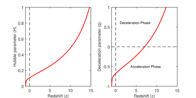
Figure 1: (left) The plot of $H$ versus $z$, (right) The plot of $q$ versus $z$.

Using Eqs. (29) in (25) and (26), we obtain the metric potentials as follows

$$A\left(t\right)=D_{1}\exp\left(F\right)\exp\left[-\frac{\chi_{1}}{9}\beta\left(3F+1\right)\exp\left(-3F\right)\right],$$ (36)

and

$$B\left(t\right)=D_{2}\exp\left(F\right)\exp\left[-\frac{\chi_{2}}{9}\beta\left(3F+1\right)\exp\left(-3F\right)\right].$$ (37)

Using Eqs. (32) and (33), the metric in Eq. (8) becomes as follows

$$ds^{2} = dt^{2}-D_{1}^{2}\exp\left(2F\right)\exp\left[-\frac{2\chi_{1}}{9}\beta\left(3F+1\right)\exp\left(-3F\right)\right]dx^{2}$$

$$-D_{2}^{2}\exp\left(2F\right)\exp\left[-\frac{2\chi_{2}}{9}\beta\left(3F+1\right)\exp\left(-3F\right)\right]\left[dy^{2}+dz^{2}\right].$$

The torsion scalar $T$ for the model becomes

$$T=\frac{-6}{\beta^{2}F^{2}}-2\chi_{2}\left(2\chi_{1}+\chi_{2}\right)\exp\left(-6F\right).$$ (39)

V Physical and geometrical properties of the model

The directional Hubble parameters, which determine the expansion rate of the Universe, are given by

$$H_{1}=\chi_{1}\exp\left(-3F\right)+\frac{1}{\beta F},$$ (40)

$$H_{2}=H_{3}=\chi_{2}\exp\left(-3F\right)+\frac{1}{\beta F}.$$ (41)

The expansion scalar $\theta$ and the shear $\sigma^{2}$ are obtained as

$$\theta=3H=\frac{3}{\beta F},$$ (42)

$$\sigma^{2}=\frac{1}{2}\left(\frac{\chi_{1}^{2}+2\chi_{2}^{2}}{a^{6}}\right)=\frac{1}{2}\left(\chi_{1}^{2}+2\chi_{2}^{2}\right)\exp\left(-6F\right).$$ (43)

Using Eq. (29) into Eq. (15) we get the spatial volume as

$$V=\exp\left(3F\right).$$ (44)

The average anisotropy parameter $A_{m}$ is given as

$$A_{m}=\frac{1}{3}\left(\chi_{1}^{2}+2\chi_{2}^{2}\right)\beta^{2}F^{2}\exp\left(-6F\right).$$ (45)

From Eq. (44), it is clear that the spatial volume of the model is finite at the initial singularity (i.e. at $t=0$) and approaches infinity as $t\rightarrow\infty$. Moreover, the average scale factor $a\left(t\right)$ in Eq. (29) is also finite at the early epoch of the Universe. It shows that the obtained model of the Universe is expanding continuously with cosmic time $t$. Eqs. (40)-(43) show the directional Hubble parameters $H_{i}$, the scalar expansion $\theta$ and the scalar shear $\sigma^{2}\rightarrow 0$ as $t\rightarrow\infty$ and they approach finite value as $t\rightarrow 0$. Finally, from Eq. (45), we observe that the average anisotropy parameter $A_{m}\rightarrow 0$ as $t\rightarrow\infty$. This indicates that our model contains a transition from the early anisotropic Universe to the current isotropic Universe as shown by observational data.

Using Eqs. (36) and (37) in the field equations (11)-(13), with simple math, the physical parameters such as energy density $\rho\left(t\right)$, cosmic pressure $p\left(t\right)$ are obtained as

$$\rho\left(t\right)=\frac{12}{\beta^{2}F^{2}}+4\chi_{2}\left(2\chi_{1}+\chi_{2}\right)\exp\left(-6F\right)$$ (46)

$$p\left(t\right)=\frac{8}{\beta^{2}F^{3}}+\frac{24\chi_{2}}{\beta F}\exp\left(-3F\right)-12\left\{\chi_{2}\exp\left(-3F\right)+\frac{1}{\beta F}\right\}^{2}$$ (47)

Using the relationship between cosmic time $t\left(z\right)$ and redshift $z$ in Eq. (33) and Eqs. (46) and (47), we plot the behavior of the energy density $\rho\left(z\right)$ and pressure $p\left(z\right)$ of the Universe versus redshift $z$ in Fig. 2, respectively. First of all, note that $\rho\left(z\right)$ and $p\left(z\right)$ $\rightarrow 0$ as $z\rightarrow-1$ (or $t\rightarrow\infty$), which is similar behavior to the big-bang model. From Fig. 2 (left), we can observe that the energy density remains positive throughout the evolution of the Universe and is a decreasing function of redshift $z$. The pressure in Fig. 2 (right), evolves from early positive values to present negative ones. As per the observation, the negative pressure is due to DE in the context of accelerated expansion of the Universe. Hence, the behavior of pressure in our model is consistent with this observation.

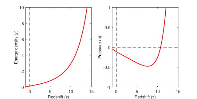
Figure 2: (left) The plot of $\rho$ versus $z$, (right) The plot of $p$ versus $z$.

Using the equation of state for a perfect fluid $\left(\omega=\frac{p}{\rho}\right)$, and using Eqs. (46) and (47), we find the EoS parameter as follows

$$\omega\left(t\right)=\frac{\frac{2}{\beta^{2}F^{3}}+\frac{6\chi_{2}}{\beta F}\exp\left(-3F\right)-3\left\{\chi_{2}\exp\left(-3F\right)+\frac{1}{\beta F}\right\}^{2}}{\frac{3}{\beta^{2}F^{2}}+\chi_{2}\left(2\chi_{1}+\chi_{2}\right)\exp\left(-6F\right)}$$ (48)

The EoS parameter is among the basic tools for studying the different phases of the Universe as well as the history of the Universe. If $\omega=-1$, it represents $\Lambda CDM$ model, $-1<\omega<-\frac{1}{3}$, represents quintessence model and $\omega<-1$, indicates phantom behavior of the model. We have plotted the EoS parameter $\omega\left(z\right)$ for redshift $z$ in Fig. 3 (left) for a fixed value of the pair $\left(\beta,c\right)$, the EoS parameter $\omega\in$ quintessence region for high redshift $z$ and over time, $\omega\rightarrow-1$ in infinite future (i.e. $z\rightarrow-1$). The present value of the EoS parameter of our model is consistent with the observational data on $\omega$ from Planck data ref47 :

• $\omega=-1.56_{-0.84}^{+0.60}$ (Planck + TT + lowE),

• $\omega=-1.58_{-0.41}^{+0.52}$ (Planck + TT, EE + lowE),

• $\omega=-1.57_{-0.40}^{+0.50}$ (Planck + TT, TE, EE + lowE + lensing),

• $\omega=-1.04_{-0.10}^{+0.10}$ (Planck + TT, TE, EE + lowE + lensing + BAO).

From Fig. 3 (left), it is clear that the EoS parameter of our model is within the range of the above observational data. Accordingly, our results are in agreement with previous observational data.

Figure 3: (left) The plot of $\omega$ versus $z$, (right) The plot of energy conditions versus $z$.

V.1 Energy Conditions

Energy conditions are a set of conditions that describe matter in the Universe and are used in many approaches to understanding the evolution of the Universe. The role of energy conditions is to verify the acceleration of the expansion of the Universe. There are many forms of energy conditions such as null energy condition (NEC), weak energy condition (WEC), dominant energy condition (DEC), and strong energy condition (SEC). Here ref48 ; ref49 ; ref50 ; ref51 ; ref52 , a group of authors who have done work on energy conditions. In $f(T)$ gravity with known energy density and pressure, these energy conditions are given as follows

• WEC: $\rho\geq 0$

• NEC: $\rho+p\geq 0$

• DEC: $\rho-p\geq 0$

• SEC: $\rho+3p\geq 0$

Fig. 3 (right) represents the energy conditions as a function of time for our model under study, i.e. the Bianchi type-I Universe with the DP varies with cosmic time as a linear function of the Hubble parameter $H$. From the figure below, we notice that the WEC, NEC, and DEC are well satisfied throughout the cosmic evolution, while there is a clear violation of the SEC. Thus, the violation of the SEC gives us the acceleration of the Universe.

V.2 Perturbation and stability of the obtained solution

To study the stability of our solutions, we will follow the same approach found in this work ref53 ; ref54 . We will use the perturbation approach to check the obtained expanding background solution stability against perturbation of scale factors or the metric field. Now, we will consider the existence of a perturbation for the three scale factors $a_{i}\left(i=1,2,3\right)$ as

$$a_{i}\longrightarrow a_{B_{i}}+\delta a_{i}=a_{B_{i}}\left(1+\frac{\delta a_{i}}{a_{B_{i}}}\right)=a_{B_{i}}\left(1+\delta b_{i}\right),$$ (49)

where $\delta b_{i}=\frac{\delta a_{i}}{a_{B_{i}}}$.

In the same way, we write the perturbation in the spatial volume $V=\prod\nolimits_{i=1}^{3}a_{i}$, directional Hubble parameters $H_{i}=\frac{\overset{.}{a_{i}}}{a_{i}}$ and mean Hubble parameter $H=\frac{1}{3}\sum_{i=1}^{3}H_{i}$ as follows

$$V\longrightarrow V_{B}+V_{B}\underset{i}{\sum}\delta b_{{}_{i}},$$ (50)

$$H_{i}\longrightarrow H_{B_{i}}\underset{i}{+\sum}\delta b_{{}_{i}},$$ (51)

$$H\longrightarrow H_{B}+\frac{1}{3}\underset{i}{\sum}\delta b_{{}_{i}}.$$ (52)

Here, $V_{B}$, $H_{B_{i}}$ and $H_{B}$ are the background spatial volume, directional Hubble parameters, and mean Hubble parameter respectively. Now, it can be shown that the metric linear order perturbations $\delta b_{{}_{i}}$ satisfy the following differential equations

$$\underset{i}{\sum}\delta\overset{..}{b}_{i}+2\underset{i}{\sum}H_{B_{i}}\delta\overset{.}{b}_{i}=0,$$ (53)

$$\delta\overset{..}{b}_{i}+\frac{\overset{.}{V}_{B}}{V_{B}}\delta\overset{.}{b}_{i}+\underset{j}{\sum}\delta\overset{.}{b}_{j}H_{B_{i}}=0,$$ (54)

$$\underset{i}{\sum}\delta\overset{.}{b}_{i}=0.$$ (55)

With a little math, we can easily find through Eqs. (53)-(55) the following relation

$$\delta\overset{..}{b}_{i}+\frac{\overset{.}{V}_{B}}{V_{B}}\delta\overset{.}{b}_{i}=0.$$ (56)

For our model, $V_{B}$ is given by

$$V_{B}=\exp\left(\frac{3}{\beta}\sqrt{2\beta t+c}\right).$$ (57)

Using the above condition in Eq. (56) and after integration, we find

$$\delta b_{i}=-c_{i}\left[\frac{\left(\beta+3\sqrt{2\beta t+c}\right)}{9\exp\left(\frac{3\sqrt{2\beta t+c}}{\beta}\right)}\right],$$ (58)

where $c_{i}$ is an integrating constant. Thus, for each scale factor $a_{i}$, the actual fluctuations are given by

$$\delta a_{i}=-c_{i}\left[\frac{\left(\beta+3\sqrt{2\beta t+c}\right)}{9\exp\left(\frac{3\sqrt{2\beta t+c}}{\beta}\right)}\right].$$ (59)

From the above equation, it is clear that $\delta a_{i}$ approaches zero as $t\rightarrow\infty$. The same behavior is illustrated by Fig. 4 (left) which represents the variation of $\delta a_{i}$ in terms of the redshift $z$, i.e. $\delta a_{i}\rightarrow 0$ as $z\rightarrow-1$. Thus, the background solution is stable against the perturbation of the metric.

V.3 Jerk parameter

As it is known in the literature, the jerk parameter is one of the fundamental physical quantities to describe the dynamics of the Universe. The Jerk parameter is a dimensionless third derivative of the scale factor $a\left(t\right)$ for cosmic time $t$ and is defined as

$$j=\frac{\overset{...}{a}}{aH^{3}}.$$ (60)

Eq. (60) can be written in terms of a DP as

$$j=q+2q^{2}-\frac{\overset{.}{q}}{H}.$$ (61)

Using Eqs. (30) and (31), the jerk parameter for our model is

$$j=\frac{3\beta^{2}}{2\beta t+c}-\frac{3\beta}{\sqrt{2\beta t+c}}+1.$$ (62)

To study the behavior of the jerk parameter $j\left(z\right)$, it is better to express it in terms of redshift $z$

$$j\left(z\right)=\frac{3}{\left(F_{0}-\log\left(1+z\right)\right)^{2}}-\frac{3}{F_{0}-\log\left(1+z\right)}+1.$$ (63)

For the $\Lambda CDM$ model, the value of the jerk parameter is $j=1$. The Universe shifts from the early deceleration phase to the current acceleration phase with a positive jerk parameter $j_{0}>0$ and a negative DP $q_{0}<0$ according to the $\Lambda CDM$ model. Fig. 4 (right) represents the variation of jerk parameter $j$ versus redshift $z$. It is very clear from this figure, that the jerk parameter remains positive throughout the cosmic evolution. The current jerk parameter value $j_{0}\left(z=0\right)$ is positive. As a result, at present $z=0$, our model can be expected to adopt the behavior of another DE model instead of the $\Lambda CDM$ model $j\neq 1$, but in the future $z\rightarrow-1$, our model is similar to the $\Lambda CDM$ model $j=1$. For comparison with observation data, the value of the jerk parameter of our model is within the range of values observed by the SNIa data $\left(j=1.32_{-1.21}^{+1.37}\right)$ ref55 , and the combined results of the SNLS project and the X-ray galaxy cluster distance measurements $\left(j=0.51_{-2.00}^{+2.55}\right)$ ref56 .

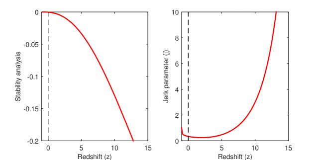
Figure 4: (left) The plot of $\delta a_{i}$ versus $z$, (right) The plot of $j$ versus $z$.

V.4 Statefinder diagnostic

The statefinder pair is a very important geometrical diagnostic tool used to distinguish different DE models such as $\Lambda CDM$, $HDE$, $CG$, $SCDM$, and $Quintessence$. The state-finder pair $\left\{r,s\right\}$ is defined as ref57

$$r=\frac{\overset{...}{a}}{aH^{3}},\text{ \ \ \ \ }s=\frac{r-1}{3\left(q-\frac{1}{2}\right)}$$ (64)

We can find different models of DE according to the values of the couple $r$ and $s$. In particular,

• $\Lambda CDM$ corresponds to $\left(r=1,s=0\right),$

• $SCDM$ corresponds to $\left(r=1,s=1\right),$

• $HDE$ corresponds to $\left(r=1,s=\frac{2}{3}\right),$

• $CG$ corresponds to $\left(r>1,s<0\right),$

• $Quintessence$ corresponds to $\left(r<1,s>0\right)$

Using Eqs. (29), (30) and (31), the values of the state-finder parameters in terms of redshift $z$ for our model are

$$r\left(z\right)=\frac{3}{\left(F_{0}-\log\left(1+z\right)\right)^{2}}-\frac{3}{F_{0}-\log\left(1+z\right)}+1$$ (65)

$$s\left(z\right)=\frac{2\left(F_{0}-\log\left(1+z\right)\right)-2}{\left[3\left(F_{0}-\log\left(1+z\right)\right)-2\right]\left(F_{0}-\log\left(1+z\right)\right)}$$ (66)

From Fig. 5, we notice that the statefinder parameters $\left\{r,s\right\}$ evolve from the CG (Chaplygin Gas) region $\left(r>1,s<0\right)$ to the quintessence region $\left(r<1,s>0\right)$ at present, and later time to $\Lambda CDM$ point $\left(r=1,s=0\right)$. As a result, our model current behaves like a quintessence model for DE.

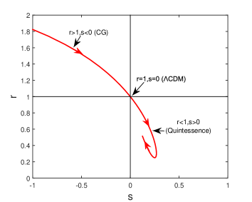
Figure 5: The plot of $(s,r)$ trajectories.

VI Discussions and conclusions

In this paper, we have studied a cosmological model with a variable deceleration parameter in a Bianchi type-I Universe in $f(T)$ gravity by assuming a particular form of the deceleration parameter as a linear function of the Hubble parameter i.e. $q=-1+\beta H$, $\beta>0$. We consider $f(T)=T$ and find the field equations for our model and graphically represent the different physical and geometric parameters as a function of the redshift. The important results of our model are:

• The DP of our model gives us two phases of the Universe, the early deceleration phase, and the current acceleration phase, as indicated by the observational data. The Hubble parameter of our model is a decreasing function of redshift $z$. Also, $H\rightarrow 0$ as $z\rightarrow-1$ (i.e. $t\rightarrow\infty$).

• Thus, our model contains a transition from the early anisotropic Universe $\left(A_{m}\neq 0\right)$ to the current isotropic Universe $\left(A_{m}=0\right)$.

• The energy density of the Universe decreases over time and remains positive throughout cosmic evolution, while the pressure starts with positive values then changes to negative values for the current time, the negative pressure is caused by cosmic acceleration.

• The EoS parameter $\omega$ of our model evolves from the quintessence region to the $\Lambda CDM$ model region in the future $\omega\rightarrow-1$.

• All the energy conditions are satisfied throughout cosmic evolution, except the SEC condition is violated, and the reason is due to cosmic acceleration.

• For the stability analysis, the background solution is stable against the perturbation of the metric.

• The jerk parameter is positive throughout the evolution of the Universe. Thus, our model can be expected to adopt the behavior of another DE model instead of the $\Lambda CDM$ model $j\neq 1$ at present $z=0$, but our model is similar to the $\Lambda CDM$ model $j=1$ in the future $z\rightarrow-1$.

• The statefinder parameters $\left\{r,s\right\}$ evolve from the CG region to the quintessence region at present, and later time to $\Lambda CDM$ point. As a result, our model behaves like the $\Lambda CDM$ model in the future.

The obtained results are similar to several works that discuss the issue of dark energy and cosmic acceleration in different contexts: $f\left(R,T\right)$ gravity, $f\left(G\right)$ gravity, $f\left(T\right)$ gravity, etc. The only difference is the choice of a different background for the study. In this reference ref58 Sharma et al. obtained similar results for our model by studying the simplest non minimal matter-geometry coupling in the framework of the $f\left(R,T\right)$ gravity with power law expansion of the scale factor. It is noticeable that such forms of the scale factor produce a constant deceleration parameter ref59 ; ref60 ; ref61 , while in the present work we chose the deceleration parameter as a linear function of the Hubble parameter which leads to the production of the deceleration parameter varies with cosmic time, such as ref41 ; ref62 .

References

- (1) Einstein, Albert. ”The general theory of relativity.” The Meaning of Relativity. Springer, Dordrecht, 1922. 54-75.
- (2) Friedman, Alexander. ”Über die krümmung des raumes.” Zeitschrift für Physik 10.1 (1922): 377-386.
- (3) Perlmutter, Saul, et al. ”Measurements* of the Cosmological Parameters and from the First Seven Supernovae at .” The astrophysical journal 483.2 (1997): 565.
- (4) Perlmutter, Saul, et al. ”Discovery of a supernova explosion at half the age of the Universe.” Nature 391.6662 (1998): 51-54.
- (5) Riess, Adam G., et al. ”Observational evidence from supernovae for an accelerating Universe and a cosmological constant.” The Astronomical Journal 116.3 (1998): 1009.
- (6) Tegmark, Max, et al. ”Cosmological parameters from SDSS and WMAP.” Physical review D 69.10 (2004): 103501.
- (7) Allen, S. W., et al. ”Constraints on DE from Chandra observations of the largest relaxed galaxy clusters.” Monthly Notices of the Royal Astronomical Society 353.2 (2004): 457-467.
- (8) Nojiri, Shin’Ichi, and Sergei D. Odintsov. ”Introduction to modified gravity and gravitational alternative for DE.” International Journal of Geometric Methods in Modern Physics 4.01 (2007): 115-145.
- (9) Nojiri, Shin’ichi, and Sergei D. Odintsov. ”Unified cosmic history in modified gravity: from theory to Lorentz non-invariant models.” Physics Reports 505.2-4 (2011): 59-144.
- (10) Nojiri, Sh, S. D. Odintsov, and VK3683913 Oikonomou. ”Modified gravity theories on a nutshell: inflation, bounce and late-time evolution.” Physics Reports 692 (2017): 1-104.
- (11) De Felice, Antonio, and Shinji Tsujikawa. ”Construction of cosmologically viable gravity models.” Physics Letters B 675.1 (2009): 1-8.
- (12) Harko, Tiberiu, et al. ” gravity.” Physical Review D 84.2 (2011): 024020.
- (13) Bamba, Kazuharu, et al. ”Finite-time future singularities in modified Gauss–Bonnet and gravity and singularity avoidance.” The European Physical Journal C 67.1 (2010): 295-310.
- (14) Myrzakulov, R., L. Sebastiani, and Sunny Vagnozzi. ”Inflation in -theories and mimetic gravity scenario.” The European Physical Journal C 75.9 (2015): 1-11.
- (15) Koussour, M., et al. ”Holographic DE in Gauss-Bonnet gravity with Granda-Oliveros cut-off.” arXiv preprint arXiv:2202.06737 (2022).
- (16) Weinberg, Steven. ”Gravitation and cosmology John Wiley & Sons Inc.” New York (1972).
- (17) Weinberg, Steven. ”The cosmological constant problem.” Reviews of modern physics 61.1 (1989): 1.
- (18) Koussour, M., and M. Bennai. ”On a Bianchi type-I space-time with bulk viscosity in gravity.” International Journal of Geometric Methods in Modern Physics (2021): 2250038.
- (19) Koussour, M., and M. Bennai. ”Interacting Tsallis holographic dark energy and tachyon scalar field dark energy model in Bianchi type-II Universe.” International Journal of Modern Physics A (2022): 2250027.
- (20) Koussour, M., and M. Bennai. ”Cosmological models with cubically varying deceleration parameter in gravity.” Afrika Matematika 33.1 (2022): 1-16.
- (21) Sharif, M., and Shamaila Rani. ” models within bianchi type-i Universe.” Modern Physics Letters A 26.22 (2011): 1657-1671.
- (22) Bhoyar, S. R., V. R. Chirde, and S. H. Shekh. ”Stability of accelerating Universe with linear equation of state in gravity using hybrid expansion law.” Astrophysics 60.2 (2017): 259-272.
- (23) Shaikh, A. Y., S. V. Gore, and S. D. Katore. ”Cosmic acceleration and stability of cosmological models in extended teleparallel gravity.” Pramana 95.1 (2021): 1-10.
- (24) Shaikh, A. Y., A. S. Shaikh, and K. S. Wankhade. ”Transist DE and thermodynamical aspects of the cosmological model in teleparallel gravity.” Pramana 95.1 (2021): 1-11.
- (25) Sharif, M., and Shamaila Rani. ”The k-essence models and cosmic acceleration in generalized teleparallel gravity.” Physica Scripta 84.5 (2011): 055005.
- (26) Shekh, S. H., and V. R. Chirde. ”Accelerating Bianchi type DE cosmological model with cosmic string in gravity.” Astrophysics and Space Science 365.3 (2020): 1-10.
- (27) Chirde, V. R., and S. H. Shekh. ”Dynamic minimally interacting holographic DE cosmological model in gravity.” Indian Journal of Physics 92.11 (2018): 1485-1494.
- (28) Boehmer, Christian G., Atifah Mussa, and Nicola Tamanini. ”Existence of relativistic stars in gravity.” Classical and Quantum Gravity 28.24 (2011): 245020.
- (29) Chirde, V. R., and S. H. Shekh. ”Barotropic bulk viscous FRW cosmological model in teleparallel gravity.” Bulgarian Journal of Physics 41.4 (2014): 258-273.
- (30) Linde, Andrei. ”Inflationary cosmology.” Inflationary Cosmology. Springer, Berlin, Heidelberg, 2008. 1-54.
- (31) Ade, Peter AR, et al. ”Planck 2013 results. XII. Diffuse component separation.” Astronomy & Astrophysics 571 (2014): A12.
- (32) Hossienkhani, Hossien, et al. ”Effects of low anisotropy on interacting holographic and new agegraphic scalar fields models of dark energy.” Physics of the dark universe 18 (2017): 17-29.
- (33) Saaidi, Kh, A. Aghamohammadi, and H. Hossienkhani. ”Modified gravity in a viscous and non-isotropic background.” Astrophysics and Space Science 341.2 (2012): 657-662.
- (34) Aghamohammadi, Ali, Hossien Hossienkhani, and Kh Saaidi. ”Anisotropy effects on baryogenesis in theories of gravity.” Modern Physics Letters A 33.13 (2018): 1850072.
- (35) Sharif, M., and M. Jamil Amir. ”Teleparallel versions of Friedmann and Lewis–Papapetrou spacetimes.” General Relativity and Gravitation 38.12 (2006): 1735-1745.
- (36) Sharif, M., and M. Jamil Amir. ”Teleparallel version of the stationary axisymmetric solutions and their energy contents.” General Relativity and Gravitation 39.7 (2007): 989-1002.
- (37) Hayashi, Kenji, and Takeshi Shirafuji. ”New general relativity.” Physical Review D 19.12 (1979): 3524.
- (38) Tiwari, R. K., A. Beesham, and B. K. Shukla. ”Cosmological models with viscous fluid and variable deceleration parameter.” The European Physical Journal Plus 132.1 (2017): 1-9.
- (39) Garg, Pryanka, Rashid Zia, and Anirudh Pradhan. ”Transit cosmological models in FRW Universe under the two-fluid scenario.” International Journal of Geometric Methods in Modern Physics 16.01 (2019): 1950007.
- (40) TIWARY, RK, Rameshwar Singh, and B. K. Shukla. ”A cosmological model with variable deceleration parameter.” The African Review of Physics 10 (2016).
- (41) Sharma, Umesh Kumar, et al. ”Stability of LRS Bianchi type-I cosmological models in gravity.” Research in Astronomy and Astrophysics 19.4 (2019): 055.
- (42) Tiwari, Rishi Kumar, Aroonkumar Beesham, and Bhupendra Kumar Shukla. ”Scenario of two-fluid DE models in Bianchi type-III Universe.” International Journal of Geometric Methods in Modern Physics 15.11 (2018): 1850189.
- (43) Garg, Priyanka, Archana Dixit, and Anirudh Pradhan. ”Cosmological models of generalized ghost pilgrim DE (GGPDE) in the gravitation theory of Saez–Ballester.” International Journal of Geometric Methods in Modern Physics (2021): 2150221.
- (44) Cunha, Joao Vital. ”Kinematic constraints to the transition redshift from supernovae type Ia union data.” Physical Review D 79.4 (2009): 047301.
- (45) Giostri, R., et al. ”From cosmic deceleration to acceleration: new constraints from SN Ia and BAO/CMB.” Journal of Cosmology and Astroparticle Physics 2012.03 (2012): 027.
- (46) Amirhashchi, Hassan, and Soroush Amirhashchi. ”Constraining Bianchi type I Universe with type Ia supernova and H (z) data.” Physics of the Dark Universe 29 (2020): 100557.
- (47) Aghanim, Nabila, et al. ”Planck 2018 results-VI. Cosmological parameters.” Astronomy & Astrophysics 641 (2020): A6.
- (48) Liu, D., & Reboucas, M. J. (2012). Energy conditions bounds on gravity. Physical Review D, 86(8), 083515.
- (49) Sadeghi, J., Banijamali, A., & Vaez, H. (2012). Constraining Gravity Models Using Energy Conditions. International Journal of Theoretical Physics, 51(9), 2888-2899.
- (50) Barcelo, C., & Visser, M. (2002). Twilight for the energy conditions?. International Journal of Modern Physics D, 11(10), 1553-1560.
- (51) Jawad, A., Pasqua, A., & Chattopadhyay, S. (2013). Correspondence between gravity and holographic DE via power-law solution. Astrophysics and Space Science, 344(2), 489-494.
- (52) Santos, C. S., Santos, J., Capozziello, S., & Alcaniz, J. S. (2017). Strong energy condition and the repulsive character of gravity. General Relativity and Gravitation, 49(4), 50.
- (53) Chen, Chiang-Mei, and Win-Fun Kao. ”Stability analysis of anisotropic inflationary cosmology.” Physical Review D 64.12 (2001): 124019.
- (54) Kao, Win-Fun. ”Bianchi type-I space and the stability of the inflationary Friedmann-Robertson-Walker solution.” Physical Review D 64.10 (2001): 107301.
- (55) Astier, Pierre, et al. ”The Supernova Legacy Survey: measurement of, and w from the first year data set.” Astronomy & Astrophysics 447.1 (2006): 31-48.
- (56) Rapetti, David, et al. ”A kinematical approach to DE studies.” Monthly Notices of the Royal Astronomical Society 375.4 (2007): 1510-1520.
- (57) Sahni, Varun, et al. ”Statefinder—a new geometrical diagnostic of DE.” Journal of Experimental and Theoretical Physics Letters 77.5 (2003): 201-206.
- (58) Sharma, Lokesh Kumar, et al. ”Non-minimal matter-geometry coupling in Bianchi I space-time.” Results in Physics 10 (2018): 738-742.
- (59) Bishi, Binaya K., et al. ”LRS Bianchi type-I cosmological model with constant deceleration parameter in gravity.” International Journal of Geometric Methods in Modern Physics 14.11 (2017): 1750158.
- (60) V. R. Chirde, S. H. Shekh. Transition between general relativity and quantum gravity using quark and strange quark matter with some kinematical test, J. Astrophys. Astr. (2018) 39:56
- (61) Shekh, S. H., and V. R. Chirde. ”Analysis of general relativistic hydrodynamic cosmological models with stability factor in theories of gravitation.” General Relativity and Gravitation 51.7 (2019): 1-22.
- (62) Hossienkhani, H., H. Yousefi, and N. Azimi. ”The effects of anisotropy on the simplest non-minimal coupling between curvature and matter in gravity.” Canadian Journal of Physics 97.9 (2019): 966-973.