Label-efficient Hybrid-supervised Learning for Medical Image Segmentation

Abstract

Due to the lack of expertise for medical image annotation, the investigation of label-efficient methodology for medical image segmentation becomes a heated topic. Recent progresses focus on the efficient utilization of weak annotations together with few strongly-annotated labels so as to achieve comparable segmentation performance in many unprofessional scenarios. However, these approaches only concentrate on the supervision inconsistency between strongly- and weakly-annotated instances but ignore the instance inconsistency inside the weakly-annotated instances, which inevitably leads to performance degradation. To address this problem, we propose a novel label-efficient hybrid-supervised framework, which considers each weakly-annotated instance individually and learns its weight guided by the gradient direction of the strongly-annotated instances, so that the high-quality prior in the strongly-annotated instances is better exploited and the weakly-annotated instances are depicted more precisely. Specially, our designed dynamic instance indicator (DII) realizes the above objectives, and is adapted to our dynamic co-regularization (DCR) framework further to alleviate the erroneous accumulation from distortions of weak annotations. Extensive experiments on two hybrid-supervised medical segmentation datasets demonstrate that with only 10$\%$ strong labels, the proposed framework can leverage the weak labels efficiently and achieve competitive performance against the 100$\%$ strong-label supervised scenario.

Introduction

Figure 1: Top: Strongly and weakly-annotated instances of endoscopic images and polyp annotations. There are varied distortion levels in the weak annotations, e.g., fairly good (col. 2), slightly distorted (col. 3-4), and completely incorrect (col. 5). Bottom: Test instances and probability maps produced by self-correcting network (Ibrahim et al. 2020), strong-weak network (Luo and Yang 2020) and our method.

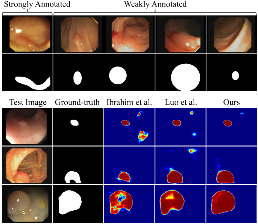
Medical image segmentation has always been a fundamental task in various biomedical applications, aiming at identifying critical anatomic or pathological structures for further statistical analysis. Although significant improvements have been made in recent works (Ronneberger, Fische, and Brox 2015), the performance of the deep learning models is strongly impacted by the extensive high-quality annotations, which are expertise-demanding, labor-intensive, and time-consuming, thus hindering deep learning technology from the real-world clinical usages.

Recent studies (Bearman et al. 2016; Lin et al. 2016) on weakly supervised semantic segmentation demonstrate that weak annotations (e.g., image-level labels, bounding boxes, scribbles) also have the competence of extracting the generalized features compared with strong annotations. Thus, a flurry of techniques (Wei et al. 2018; Lee et al. 2019) have been explored to utilize only a few pixel-wise strong labels as guidance to learn fine-grained representations for segmentation. However, as all the strongly- and weakly-annotated instances are treated equally in such solutions, a large number of pseudo labels with less precise depiction capability inevitably dominate the training process, leading to an inferior and less reliable performance (Luo and Yang 2020).

The key issue responsible for the poor performance of these solutions is the inherent inconsistency between weak and strong annotations. Specifically, the weakly-annotated instances contain a large number of low-quality semantic cues, while the strongly-annotated instances provide scarce yet fine-grained priors. To tackle this issue and utilize both annotations more efficiently, some efforts proposed multi-branch networks (Luo and Yang 2020) or dual networks (Ibrahim et al. 2020; Ning et al. 2020), which handle two types of supervision separately. Specifically, they designed specific approach to interact across strongly and weakly supervised branches, such as self-correction module (Ibrahim et al. 2020), shared backbone (Luo and Yang 2020), and exponential moving average (Ning et al. 2020), which can alleviate the problem of supervision inconsistency to some extent.

However, the mutual information is still hard to compromise across two parallel branches learned from weakly- and strongly-annotated instances, and thus the over-guiding problem raised by a single type of supervision often exists. On the other hand, as these multi-branch frameworks holistically tackle the supervision inconsistency, the instance inconsistency within the weakly-annotated subset is completely ignored. In fact, weakly-annotated instances usually contain varying degrees of imaging and annotation distortion (see Fig. 1), which can sometimes mislead the representation learning process and thus low down the model’s generalization capability. For example, a completely incorrect annotation from weakly-annotated subset undoubtedly hurts the overall performance, while a slightly distorted one can provide fairly valuable guidance to the model learning. In this case, concentrating on supervision inconsistency while ignoring the instance inconsistency makes the overall trade-off between strongly and weakly supervised branches more intractable, leading to undesirable results (see Fig. 1 (bottom)).

To address above issues, we propose a novel label-efficient hybrid-supervised framework regarding the medical semantic segmentation task, which learns a series of dynamic instance indicators (DII) to reweight each weakly-annotated instance individually under the guidance from strongly-annotated instances. The learned DII estimates the instance importance, e.g., instances with slight distortions should be granted more attention, while instances with severe annotation distortions will be down-weighted. In this way, rich and valuable semantic cues contained in massive weakly-annotated instances can be efficiently exploited, while the negative impact is mitigated. The main contributions of this study can be summarized as follows:

• To the best of our knowledge, we are the first to reveal the inconsistency among weakly-annotated instances that obstructs the exploitation of weak annotations in a hybrid-supervised semantic setting.

• To tackle the obstacle of instance inconsistency, we introduce the DII, which learns a separate weight for each of weakly-annotated instances guided by the gradient direction of strongly-annotated instances.

• To further exploiting the fruitful semantic clues from noisy weakly-annotated instances, we design a dynamic co-regularized (DCR) architecture with the aid of DII. DCR provides a powerful regularization effect and consequently helps avoid erroneous accumulation from the distortion within weak annotations.

• Extensive experiments and analysis on the CVC-EndoSceneStill and AS-OCT datasets demonstrate that when only a few strongly-annotated instances are given, our framework has the competence to learn from extensive weakly-annotated instances and achieves the performance close to that of the corresponding fully supervised version.

Related Work

Weakly Supervised Semantic Segmentation.

Weakly supervised semantic segmentation aims to reduce the annotation efforts by leverage low-cost labels (Lin et al. 2016; Dai, He, and Sun 2015; Bearman et al. 2016). These approaches are generally optimized the network and the graphical model alternatively and customized to the specific dataset. For instance, region growing (Huang et al. 2018), CRF (Krähenbühl and Koltun 2011) and GrabCut (Rother, Kolmogorov, and Blake 2004) were employed to constrain the segmentation to coincide with object boundaries. However, since the graphical model requires definite boundaries between objects, the efficacy of such schemes are doubtful when applying to the medical image dataset.

Hybrid-supervised Semantic Segmentation.

Hybrid-supervised semantic segmentation introduces few strong annotations combined with weak ones, aiming at provide fine-grained guidance and thus improving the segmentation performance (Papandreou et al. 2015). For example, generative adversarial network based approaches (Souly, Spampinato, and Shah 2017) fused pixel-level labeled data and image-level labeled data through adversarial objectives. Multi-stage approaches bundled the strong supervision and the proxy supervision estimated from weakly supervised models to learn a single network in the last stage (Wei et al. 2018; Lee et al. 2019). However, the equal treatment of inconsistent annotated data may allow weakly-annotated instances overwhelm the strongly-annotated ones limited in sample numbers, which in turn produces worse results (Luo and Yang 2020).

To separately use weak annotations and strong ones, a self-correcting network was proposed (Ibrahim et al. 2020). It trained a primary and an ancillary network and fused features from these two networks via a self-correcting module. More recently , a strong-weak network  (Luo and Yang 2020) was proposed to use a shared backbone to exploit the joint information. Marco-micro framework (Ning et al. 2020) leveraged the uncertainty-aware consistency and the mean-teacher to provide reliable guidance for both marco and micro branches. Indeed, these subtle dual-branch approaches accompanied by dedicated mutual interactions that avoided overwhelming the handful yet vital minority and consequently led to compelling performance to some extent. However, as discussed in the previous section, these interactions only address holistic inconsistency between datasets while ignoring instance inconsistency.

Figure 2: Overview of our proposed label-efficient hybrid-supervised learning framework, which alternatively updates the upper-level DIIs ($\Gamma$) and the lower-level DCR networks (${\theta}$). Left: Upper-level computation graph, which estimates the upper-level gradient $\frac{\partial\mathcal{L}(\mathcal{D}_{S},\theta^{*}(\Gamma))}{\partial\gamma_{k}}$ w.r.t. DII $\gamma_{k}$ guided by the strongly-annotated instances ${X}_{S}$ (refer to Eq. 3) and updates $\gamma_{k}$ using gradient descent. Right: Lower-level dual-network DCR framework, where each network is supervised by a designed tutorial and estimates a pseudo segmentation map to supervise the other network.

Method

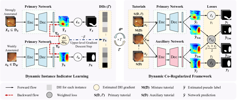
Fig. 2 illustrates our proposed hybrid-supervised segmentation framework, which iteratively alternates between upper-level DII and lower-level DCR learning steps. The upper-level DII learns an individual weight for each weakly-annotated instance via the gradient-based method. The lower-level DCR framework, on the other hand, employs the dual network structure and is trained in a co-regularized manner, where each network is not only supervised by the corresponding annotation but also by the pseudo mask generated from the other branch.

Problem Formulation

In our hybrid-supervised medical image segmentation, the training set $\mathcal{D}$ consists of a strongly-annotated subset $\mathcal{D}_{S}=\{(\mathbf{x}_{k},\mathbf{y}_{k})|1\leq k\leq N\}$ with manual pixel-wise delineations and a weakly-annotated subset $\mathcal{D}_{W}=\{(\mathbf{x}_{k},\mathbf{y}_{k})|1\leq k\leq M\}$ including coarse and noisy masks, where $\mathbf{x}\in\mathbb{R}^{H\times W\times 3}$ is an input image with size $H\times W\times 3$, $\mathbf{y}\in\{0,1\}^{H\times W\times C}$ is a corresponding mask with $C$ categories, and $N\ll M$. The core concept of our method is to build a segmentation framework parameterized by $\theta$ and achieves decent performance when learning from massive weakly-annotated instances and minimum strongly-annotated instances. We denote the overall objective function of a set of instances $X$ as $\mathcal{L}(X,\theta)$ and the loss of the $i$-th instance as $\ell(\mathbf{x}_{i},\mathbf{y}_{i},\theta)$.

Dynamic Instance Indicator Learning

As mentioned before, the distortion of weak annotations introduces the supervision inconsistency and instance inconsistency, posing a major challenge to the efficient and reasonable utilization of weakly- and strongly-annotated data. To this end, our dynamic instance indicator (DII) is proposed to consider each weakly-annotated instance individually instead of making a global trade-off between weak and strong supervision information like existing methods (Luo and Yang 2020; Ning et al. 2020). Intuitively, DII indicates the importance of each weakly-annotated instance and reflects the degree of distortion in a weak annotation.

Specifically, DII comprises a series of learnable indicators $\Gamma=\{\gamma_{k}|\gamma_{k}\in[0,1],k\in[1,M]\}$ tailored to $M$ weakly-annotated instances. Note that here we assign a constant value $\mathbf{1}_{N}$ for $N$ strongly-annotated instances.

To learn such large-scale hyperparameters, we formulate this problem as a bi-level optimization (Dempe 2020) objective, presented as:

$$\min_{\Gamma}\mathcal{L}(\mathcal{D}_{S},\theta^{*}(\Gamma)),\;s.t.\;\theta^{*}(\Gamma)=\arg\min_{\theta}\mathcal{L}(\mathcal{D},\theta,\Gamma),$$ (1)

where $\mathcal{D}=\mathcal{D}_{W}\cup\mathcal{D}_{S}$ denotes the entire dataset, and thus the lower-level loss could be expanded as $\mathcal{L}(\mathcal{D},\theta,\Gamma)=\frac{1}{N}\sum_{i=1}^{N}\ell(\mathbf{x}_{i},\mathbf{y}_{i},\theta)+\frac{1}{M}\sum_{k=1}^{M}\gamma_{k}\ell(\mathbf{x}_{k},\mathbf{y}_{k},\theta)$. Intuitively, the lower-level objective optimizes the network parameters $\theta$ to minimize the weighted loss over the entire dataset, while the upper-level objective tries to find the optimal indicators $\Gamma$ based on the performance of strongly-annotated subset $\mathcal{D}_{S}$.

To solve the above bi-level objectives, we utilize the adaptive gradient descent method (Kingma and Ba 2015) to tune both upper-level DIIs $\Gamma$ and lower-level parameters $\theta$. Gradient descent methods have been widely adopted for deep network and hyperparameter learning (Bengio 2000; Kingma and Ba 2015) and have shown promising performance. Here, as summarized in Algorithm 1, our method iteratively alternates between lower-level network training and upper-level DII updating steps. At every training iteration, the lower-level step trains the network parameters $\theta$ by gradient descent while fixing the indicators $\Gamma$ (line 4). After having trained the lower-level network $\tau$ steps, we perform a gradient descent step on the upper-level DIIs $\Gamma$ (line 15). These two steps are iterated $T$ times and the loss $\mathcal{L}(\mathcal{D}_{S},\theta^{*}(\Gamma))$ on strongly-annotated subset is expected to reach convergence by adjusting DIIs of weakly-annotated instances.

DII Gradient Estimation.

The crux of the above algorithm is how to compute upper-level gradient $\frac{\partial\mathcal{L}(\mathcal{D}_{S},\theta^{*}(\Gamma))}{\partial\gamma_{k}}$ for DII $\gamma_{k}$ to apply gradient descent updating. We first decompose the upper-level gradient as:

$$\frac{\partial\mathcal{L}(\mathcal{D}_{S},\theta^{*}(\Gamma))}{\partial\gamma_{k}}=\nabla_{\theta}\mathcal{L}\left(\mathcal{D}_{S},\theta^{*}(\Gamma)\right)^{\top}\cdot\ \frac{\partial\theta^{*}(\Gamma)}{\partial\gamma_{k}}.$$ (2)

Since $\theta$ is a function resulting from the previous optimization with dependencies on $\Gamma$, the calculation of upper-level gradient w.r.t. $\gamma_{k}$ requires differentiating the lower-level optimization procedure (i.e., $\arg\min_{\theta}\mathcal{L}(\mathcal{D},\theta,\Gamma)$), which turns to be intractable in practice.

To tackle the above problem, we then estimate the gradient with the established approximation method (Koh and Liang 2017). Assume that $\mathcal{L}$ is second-order differentiable and strictly convex w.r.t. $\theta$, then Eq. 2 can be estimated as:

$$\frac{\partial\mathcal{L}(\mathcal{D}_{S},\theta^{*}(\Gamma))}{\partial\gamma_{k}}=-\nabla_{\theta}\mathcal{L}\left(\mathcal{D}_{S},\theta^{*}\right)^{\top}H_{\theta}^{-1}\nabla_{\theta}\ell(\mathbf{x}_{k},\mathbf{y}_{k},\theta^{*}),$$ (3)

where $H_{\theta}=\nabla^{2}_{\theta}\mathcal{L}(\mathcal{D},\theta^{*},\Gamma)$ is the Hessian.

However, it is still impractical to compute Eq. 3 directly for existing segmentation networks as: 1) computing the Hessian involves second-order gradients, and the complexity of its inverse is far worse than the quadratic one; 2) the update of indicators $\Gamma$ requires the per-instance gradient of the loss function $\mathcal{L}$ w.r.t. huge network parameters $\theta$.

To this end, we utilize several policies to alleviate the computational burden. First of all, we use identity matrix $I$ to approximate the Hessian, as it is positive definite by assumption (Cook and Weisberg 1982). Then, we choose a subset of the network parameters (e.g., parameters from the final layer (Ren, Yeh, and Schwing 2020)) $\theta^{\prime}\subset\theta$ for gradient computation. According to the linearity of gradients, the gradient graph of the batch data can be unrolled (Ren et al. 2018), and thus batch acceleration can also be employed.

On the basis of the above approximation, the estimated upper-level gradient $\frac{\partial\mathcal{L}(\mathcal{D}_{S},\theta^{*}(\Gamma))}{\partial\gamma_{k}}$ actually reflects the “dissimilarity” of the network gradients between $k$-th weakly-annotated instance and the strongly-annotated instances. To be more specific, if the gradient direction from $k$-th weakly-annotated instance is consistent with the strongly-annotated instances, then this instance is beneficial for semantic representation learning and $\gamma_{k}$ will be larger after performing the gradient descent step.

Algorithm 1 DII Learning

0:  strongly-annotated dataset $\mathcal{D}_{S}$, weakly-annotated dataset $\mathcal{D}_{W}$, DIIs $\Gamma=\{\gamma_{k}|\gamma_{k}\in[0,1],k\in[1,M]\}$, network parameters $\theta$, DII update interval $\tau$, iteration steps $T$, and learning rates $\alpha,\beta$.

1:  for $t\leftarrow 1...T$ do

2:     $X_{batch}\leftarrow\text{BatchSample}(\mathcal{D}_{S}\cup\mathcal{D}_{W})$

3:     // Lower-level (DCR) gradient descent step

4:     $\theta\leftarrow\theta-\alpha\cdot\nabla_{\theta}\mathcal{L}(X_{batch},\theta,\Gamma)$

5:     if  $(t\mod\tau)\neq 0$ then

6:        continue

7:     end if

8:     $\theta^{*}\leftarrow\theta$

9:     $X_{S}\leftarrow\text{BatchSample}(\mathcal{D}_{S})$

10:     // Estimate mean gradients on $\mathcal{D}_{S}$

11:     $\mathbf{g}_{S}\leftarrow\nabla_{\theta}\mathcal{L}(X_{S},\theta^{*})$

12:     // Calculate per-instance gradients on $\mathcal{D}_{W}$

13:     $\mathbf{g}_{k}\leftarrow\nabla_{\theta}\ell(\mathbf{x}_{k},\mathbf{y}_{k},\theta^{*}),\;\forall k\in\{1,...,M\}$

14:     // Estimate inverse Hessian matrix

15:     $H^{-1}_{\theta}\leftarrow I$

16:     // Estimate upper-level gradients w.r.t. DIIs

17:     $\frac{\partial\mathcal{L}(X_{S},\theta^{*}{(\Gamma)})}{\partial\gamma_{k}}\leftarrow-\mathbf{g}_{S}^{\top}H^{-1}_{\theta}\cdot\mathbf{g}_{k},\;\forall k\in\{1,...,M\}$

18:     // Upper-level gradient descent step

19:     $\gamma_{k}\leftarrow\gamma_{k}-\beta\cdot\frac{\partial\mathcal{L}(X_{S},\theta^{*}{(\Gamma)})}{\partial\gamma_{k}},\;\forall k\in\{1,...,M\}$

20:  end for

Dynamic Co-Regularized Framework

Although DII reweights the instances with different degree of distortions, non-zero weights are assigned to most of weakly-annotated instances. The distortions in weak annotations can be easily imitated and accumulated with the back-propagation of gradient flows from the deeper to the lower layers (Araslanov and Roth 2020). Co-teaching (Han 2018; Wei et al. 2020) and disagreement-based learning (Yu and et al. 2019) has been utilized to alleviate the noise accumulation from the data label. Inspired by the similar concept, we propose a dynamic co-regularized (DCR) framework aided by DII to avoid the erroneous accumulation.

As shown in Fig. 2 (right), DCR is a dual-network architecture, where the primary network has the same architecture as it is in DII. For the auxiliary network, we employ the identical architecture of the primary network but with different initialization. DCR enforces the consistency on the predictions of two networks, where pseudo labels inferred from one network are used to supervise the other network. The strength of consistency regularization depends on the disagreement or diversity of two networks (Yu and et al. 2019). To prevent two networks from converging close to each other too quickly, we construct two sampling-based tutorials and a mixture tutorial as our collaborative scheme.

In specific, both the primary and auxiliary tutorials contain training pairs drawn from the hybrid dataset $\mathcal{D}$. The primary tutorial samples instances from the multinomial probability distribution corresponding to the DII weights, denoted as $S(\mathcal{D},\Gamma)$. In contrast, the auxiliary tutorial uses uniform random sampling. The collaborative training scheme demands an extra input from mixture tutorial (a.k.a, $\mathbf{x}_{m}$) for the consistency regulation. Here, cutmix (Yun et al. 2019) is the optimal option to form the mixture tutorial in our study. We create the mixture tutorial by pasting the foreground regions specified by the given ground truth mask from the image of primary tutorial to the image of auxiliary tutorial. The same operation will be performed consistently to the corresponding pseudo mask as well. More details are described as follows.

Given an image $\mathbf{x}_{i}$ with annotation $\mathbf{y}_{i}$ from the primary tutorial, we randomly select a class $c$ in $\mathbf{y}_{i}$ and extract its binary mask $B^{c}_{i}$. The mixed image can be defined as:

$$\mathbf{x}_{m}=B^{c}_{i}\odot\mathbf{x}_{i}+(1-B^{c}_{i})\odot\mathbf{x}_{j},$$ (4)

where $\mathbf{x}_{j}$ is an image from the auxiliary tutorial and $\odot$ denotes element-wise multiplication. The image from mixture tutorial $\mathbf{x}_{m}$ is fed into two networks. The consistency regulation in DCR constrains two network outputs through the regularization loss:

$$r_{i,j}=\ell(\mathbf{x}_{m},\tilde{\mathbf{y}}_{2m},\theta_{1})+\ell(\mathbf{x}_{m},\tilde{\mathbf{y}}_{1m},\theta_{2}),$$ (5)

where $\theta_{1}$ and $\theta_{2}$ denote parameters of two networks, and $\tilde{\mathbf{y}}_{1m}$ and $\tilde{\mathbf{y}}_{2m}$ are the pseudo masks generated from two networks. Taking $\tilde{\mathbf{y}}_{1m}$ as an example, we feed $\mathbf{x}_{i}$ and $\mathbf{x}_{j}$ into the primary network and then mix the predictions:

$$\tilde{\mathbf{y}}_{1m}=B^{c}_{i}\odot\hat{\mathbf{y}}_{1i}+(1-B^{c}_{i})\odot\hat{\mathbf{y}}_{1j},$$ (6)

where $\hat{\mathbf{y}}_{1i}$ and $\hat{\mathbf{y}}_{1j}$ are network predictions for images $\mathbf{x}_{i}$ and $\mathbf{x}_{j}$, respectively. This pseudo mask is utilized as the supervision for auxiliary network. Similarly, we can obtain the $\tilde{\mathbf{y}}_{2m}$ following the same step. Eventually, the lower-level loss can be written as:

$$\mathcal{L}(\mathcal{D},\theta,\Gamma)=\sum_{i,j}\gamma_{i}\ell_{i}+\gamma_{j}\ell_{j}+\lambda\cdot\frac{\gamma_{i}+\gamma_{j}}{2}r_{i,j},$$ (7)

where $\ell_{i}$ and $\ell_{j}$ are losses for primary and auxiliary networks respectively, and $\lambda$ is a hyperparameter to balance the supervised loss and the regularization loss. All losses are implemented with the vanilla pixel-wise cross-entropy loss.

Experiments

We conduct extensive experiments to verify the effectiveness of our proposed method on different types of medical segmentation tasks with varied types of weak annotations.

Datasets and Evaluation Metrics

Polyp Segmentation.

The hybrid-supervised polyp segmentation dataset has been built from two public available colonoscopic polyp datasets. The CVC-EndoSceneStill (Vázquez et al. 2017) includes 912 images with elaborately annotated pixel-level labels. We take 10% sample pairs ($55$ images) from its training set ($547$ images) as our strong priors and use its test set ($182$ images) for evaluation. Meanwhile, more than $11k$ frames across $18$ sequences are acquired from the polyp detection dataset CVC-VideoClinicDB (Angermann et al. 2017) to provide ellipse masks as weak annotations (refer to Fig. 1). Although the given weak annotations are trying to approximate the polyp shapes, the inaccurate approximation undoubtedly causes varying degrees of distortions. We also introduce artifact of the weak annotation by replacing $40\%$ polyps foreground with the background class so as to simulate unrecognized target during the human annotation.

AS-OCT Segmentation.

The hybrid-supervised AS-OCT segmentation dataset is modified from the training set of the Angle closure Glaucoma Evaluation (AGE) Challenge (Fu et al. 2019), which contains over 3200 AS-OCT images with annotations of the closure classification and the coordinates of scleral spurs. Same configurations of previous work (Ning et al. 2020) are adopted in this dataset, where two versions of annotation are entailed. The strong annotation provides the pixel-wise masks of iris and cornea, while the weak annotation is re-annotated with line strokes inside these tissues by experienced ophthalmologists. Then, we follow the same partition protocol in which $60\%$ of the data is used for training, $20\%$ for validation, and the rest $20\%$ for test. It is worth mentioning that only $1\%$ of the training instances utilize strong annotations.

Evaluation Metrics.

Dice coefficient and average symmetric surface distance (ASSD)  (Heimann et al. 2009) are utilized to measure the segmentation performance. For the polyp segmentation task, the prediction performance is reported on pathological regions. For the AS-OCT segmentation task, we report above quantitative evaluation metrics regarding the iris and cornea prediction.

Implementation Details.

We implement our algorithm based on the PyTorch framework (Paszke, Gross, and et al. 2019). The DeepLabv3+ structure (Chen et al. 2018) with a ResNet50 backbone pre-trained on ImageNet (Deng et al. 2009) is chosen as the primary branch and auxiliary branch in the proposed framework. Random initialization is applied to the parameters of decoders in two branches. In addition, $\gamma_{1},...,\gamma_{M}$ is initialized with $0.5$ and clipped to the range of $[0,1]$. We adopt vanilla Adam optimizer (Kingma and Ba 2015) to tune DIIs with default betas set to 0.9 and 0.999 respectively. Network parameters are updated iteratively via mini-batch SGD with momentum=0.9, batch size=16 and weight decay=0.00005. The upper-level and lower-level learning rates are initially set to $0.1$ and $0.002$ by default, respectively.

Model	DII	DCR	DII Sampling	Dice	ASSD
Baseline				69.77	11.29
Our Variants				72.52	10.46
				76.32	9.68
				81.15	8.14
				82.56	8.37

Table 1: Ablation studies on the polyp segmentation dataset.

DCR Variants	Dice	ASSD
Foreground Paste $\rightarrow$ CutMix	81.37	8.58
Pseudo Regularization $\rightarrow$ KL Div.	76.83	8.47
Full DCR	82.56	8.37

Table 2: Impact of foreground paste and pseudo regularization strategy on DCR performance.

(a)

(b)

(c)

Figure 3: (a): Demonstration of DIIs for randomly selected instances, where the green ellipses are weak annotations, the red box indicates missing annotation, and the numbers show the optimal DII values. DII successfully reflects “importance” of weakly-annotated instance. (b): DII distribution on weakly-annotated polyp segmentation dataset. (c): Training curves w/ and w/o DII.

Ablation Studies and Analysis

To verify the effectiveness of the proposed strategies individually, we conduct ablation studies on the polyp segmentation dataset. Firstly, as performed in Table 1, we roughly merge two types of annotations under the same supervision to train the deep model as our baseline. Four variants of strategy ablations are designed, including DII, DCR, and DII tutorial. Notable performance gains have been observed when utilizing the proposed DII or DCR individually. Furthermore, we achieve 1.41% extra improvement by applying the DII sampling tutorial additionally, suggesting that our method can effectively utilize both vital strong priors and massive weak semantic cues. After that, module ablations are constructed to verify the module effectiveness of DCR. From Table 1, we substitute cutmix for foreground paste strategy causing a 1.19% Dice drop. In addition, using the Kullback-Leibler divergence as the regularization loss results in a 5.73% performance decrease, demonstrating that the proposed module can effectively exploit noisy semantic cues from weakly-annotated instances.

Understanding DIIs.

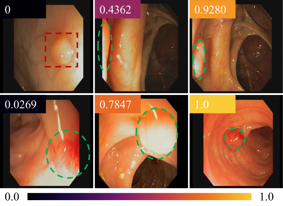
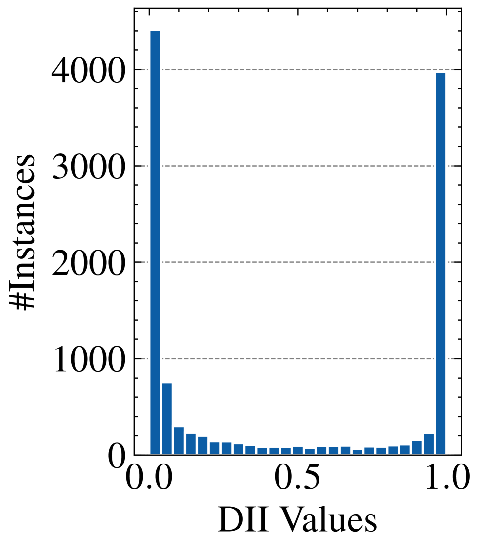
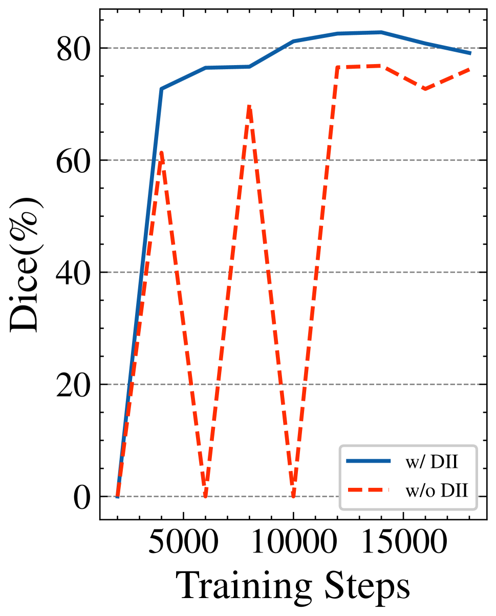
To understand what DII has learned and how it contributes to learning from weak annotations, we conduct experiment on polyp segmentation dataset and investigate its behavior. We collect learned DII values over all instances from the weakly-annotated set and then visualize several typical instances. Qualitative results are shown in Fig. 3(a). DII tries to decrease the importance of instances that contain incorrect annotations and low-quality images, and boost the importance of samples whose weak annotation is close to the ground-truth mask. We also visualize the histogram in Fig. 3(b) to reveal the relationship of the DII values and number of instances. As can be seen, most instances are pushed toward zero or one value, suggesting that DII tries to make clear useful semantic clues in weak annotations. Furthermore, Fig. 3(c) demonstrates that DII can stabilize the training procedure, since the negative effect raised from noisy annotation has been degraded along with the iterations.

(a) Performance with varied combinations of $\beta$ and $\tau$.

(b) Performance with varied regularization strength $\lambda$.

Figure 4: Experiments on different hyperparameters DII (a) and DCR (b) learning.

#Strong Annotations	28	55	110	220	546⋆
Dice	80.36	82.56	82.97	82.99	82.91
ASSD	8.42	8.37	7.76	7.32	6.52

Table 3: Experiments on different size of strongly-annotated subset. The asterisk symbol indicates fully supervised baseline (DeepLabv3+) w/o $11k$ weak annotations.

Methods	CVC-EndoSceneStill		AS-OCT
			Cornea		Iris		Mean
	Dice	ASSD	Dice	ASSD	Dice	ASSD	Dice	ASSD
Baselines
Weakly Supervised	67.43	12.66	55.14	9.30	35.03	13.62	45.09	11.46
Few Strong Supervised	67.67	12.45	78.83	5.79	68.64	6.29	73.73	6.04
Fully Supervised	82.91	6.52	95.71	0.13	91.59	0.21	93.65	0.17
Hybrid-supervised methods
FickleNet (Lee et al. 2019)	69.77	11.29	83.71	2.58	80.55	3.11	82.13	2.85
Self-Correcting (Ibrahim et al. 2020)	67.68	12.73	94.16	1.52	90.36	1.43	92.26	1.47
Marco-Micro (Ning et al. 2020)	72.33	10.74	93.93	1.58	89.79	1.61	91.86	1.60
StrongWeak (Luo and Yang 2020)	73.53	14.63	–	–	–	–	–	–
$\dagger$StrongWeak (Luo and Yang 2020)	76.41	11.42	92.15	1.85	81.68	2.62	86.91	2.24
Ours	82.56	8.37	94.39	1.35	91.81	1.19	93.10	1.27

Table 4: Quantitative comparisons with the state-of-the-art methods on the hybrid-supervised polyp segmentation dataset and AS-OCT segmentation dataset. “$\dagger$” indicates our re-implemented version with strong data augmentation for a fairer comparison.

Impact of Hyperparameters of DII and DCR.

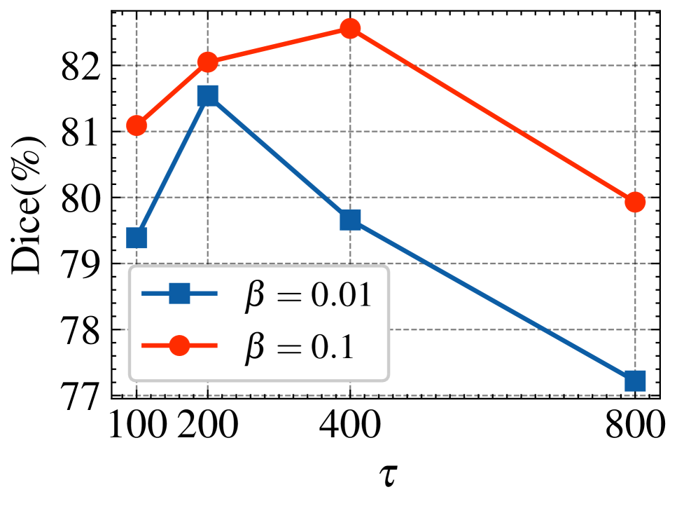
The selection of the hyper-parameters in DII and DCR can influence the learning process. Initially, we investigate the effect of update interval $\tau$ and learning rate $\beta$ in Algorithm 1 which balance the learning pace of upper-level DII and lower-level network. The result is plotted in Fig. 4(a). Unsurprisingly, we can observe that either too small or large $\tau$ will negatively affect the model performance. We finally chose the optimal configuration with $\tau=400$ and $\beta=0.1$ in our whole study.

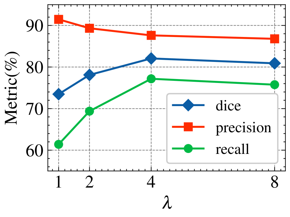
Another experiment is conducted to explore the impact of loss coefficient $\lambda$ of DCR. As illustrated in Fig. 4(b), it is noticed that the Dice score will increase at the beginning and reach the maximum at $\lambda=4$ and then decrease slowly. In addition, we also present the precision and recall curves at the same time. As the increasing of $\lambda$, we can observe the precision encounters a slight drop but the recall achieves a significant gain. We speculate that the manifestation lies in the effectiveness of the DII-guided tutorial and the foreground paste strategy which encourages the framework to predict the potential regions without overfitting. Therefore, it is inevitable to introduce few false positives that affect the precision.

Impact of the Size of Strongly-annotated Subset.

The strongly-annotated subset plays two pivotal roles in our framework: serving as a guidance in the upper-level DII learning and providing fine-grained samples in the lower-level training. Hence, the size of strongly-annotated subset on the performance needs to be investigated. Table 3 shows, unsurprisingly, that increasing strongly-annotated subset consistently improves performance. On the other hand, we find that an exponentially increase of annotation cost only obtain minor improvement in Dice score, indicating that it is worth developing efficient hybrid-supervised methods to balance annotation budget and performance.

Figure 5: Qualitative comparisons of our method with the state-of-the-arts on the polyp segmentation dataset.

Comparison with State-of-the-arts

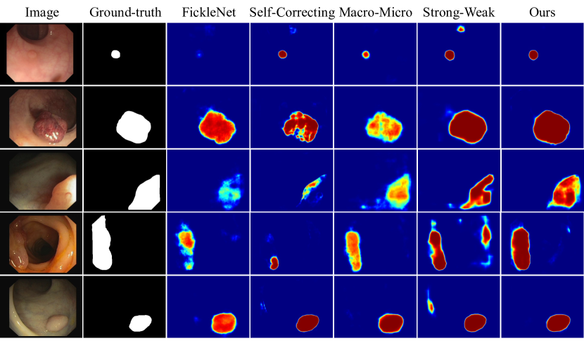
In order to verify the effectiveness of the proposed method, we compare the proposed framework with the state-of-the-art hybrid-supervised semantic segmentation methods. For fair comparison, all experimental setups are subjected to the identical experimental configurations. Specifically, three baselines of Weakly Supervised, Few Strong Supervised and Fully Supervised denote a single DeepLabv3+ network (Chen et al. 2018) trained with only weakly-annotated instances, 10% strongly-annotated instances, and 100% strongly supervised instances, respectively. Table 4 summarizes the experimental results of the proposed method, aforementioned baselines and the compared state-of-the-art methods. Our proposed method significantly outperforms all previous approaches by a large margin. In particular, our results with only 10% strongly-annotated training samples are close to that of Fully Supervised version, indicating that the fruitful semantic cues in a large number of weakly-annotated instances are exploited sufficiently. Moreover, a huge performance discrepancy on two datasets can be observed from all compared methods. In contrast, the proposed method consistently yields the best Dice scores among these methods. Fig. 5 illustrates several typical qualitative results, where less clutter or incompleteness in our results indicate that our method is more capable of exploiting semantic information in the hybrid annotated dataset.

Conclusion

This paper proposes a label-efficient hybrid-supervised learning framework for medical image segmentation, which can achieve a competitive performance by exploiting extensive weakly-annotated instances and only a handful of strongly-annotated instances. Specifically, DII learning algorithm and a DCR framework are proposed to extract the useful semantic clues and mitigate the erroneous accumulation during training. DII automatically tunes the weight for each weakly-annotated instance guided by the gradient direction from few strongly-annotated instances, which can assist the framework to overcome the instance inconsistency. Then, DCR, empowered by the collaborative training scheme and consistency regulation, further relieves the distortion in weak annotations. Extensive experiments show that the proposed method substantially outperforms current state-of-the-art approaches and reaches a close performance against the fully supervised scenario. It has great potential to serve as a reliable solution for label-efficient medical image segmentation with limited annotation.

References

- Angermann et al. (2017) Angermann, Q.; Bernal, J.; Sánchez-Montes, C.; and et al. 2017. Towards real-time polyp detection in colonoscopy videos: Adapting still frame-based methodologies for video sequences analysis. In Computer Assisted and Robotic Endoscopy and Clinical Image-Based Procedures, 29–41.
- Araslanov and Roth (2020) Araslanov, N.; and Roth, S. 2020. Single-Stage Semantic Segmentation From Image Labels. In CVPR, 4252–4261.
- Bearman et al. (2016) Bearman, A. L.; Russakovsky, O.; Ferrari, V.; and Li, F. 2016. What’s the Point: Semantic Segmentation with Point Supervision. In ECCV, volume 9911, 549–565.
- Bengio (2000) Bengio, Y. 2000. Gradient-Based Optimization of Hyperparameters. Neural Comput., 12(8): 1889–1900.
- Chen et al. (2018) Chen, L.-C.; Zhu, Y.; Papandreou, G.; Schroff, F.; and Adam, H. 2018. Encoder-Decoder with Atrous Separable Convolution for Semantic Image Segmentation. In ECCV, 833–851.
- Cook and Weisberg (1982) Cook, R. D.; and Weisberg, S. 1982. Residuals and influence in regression. New York: Chapman and Hall.
- Dai, He, and Sun (2015) Dai, J.; He, K.; and Sun, J. 2015. BoxSup: Exploiting bounding boxes to supervise convolutional networks for semantic segmentation. In CVPR, 1635–1643.
- Dempe (2020) Dempe, S. 2020. Bilevel optimization: theory, algorithms, applications and a bibliography. Springer.
- Deng et al. (2009) Deng, J.; Dong, W.; Socher, R.; Li, L.; Li, K.; and Li, F. 2009. ImageNet: A large-scale hierarchical image database. In CVPR, 248–255.
- Fu et al. (2019) Fu, H.; Li, F.; Orlando, J. I.; Bogunović, H.; Sun, X.; Liao, J.; Xu, Y.; Zhang, S.; and Zhang, X. 2019. AGE: Angle closure Glaucoma Evaluation Challenge.
- Han (2018) Han, B. 2018. Co-teaching: Robust training of deep neural networks with extremely noisy labels. In NeurIPS, 8536–8546.
- Heimann et al. (2009) Heimann, T.; van Ginneken, B.; Styner, M.; and et al. 2009. Comparison and Evaluation of Methods for Liver Segmentation From CT Datasets. IEEE TMI, 28(8): 1251–1265.
- Huang et al. (2018) Huang, Z.; Wang, X.; Wang, J.; Liu, W.; and Wang, J. 2018. Weakly-Supervised Semantic Segmentation Network With Deep Seeded Region Growing. In CVPR, 7014–7023.
- Ibrahim et al. (2020) Ibrahim, M. S.; Vahdat, A.; Ranjbar, M.; and Macready, W. G. 2020. Semi-Supervised Semantic Image Segmentation With Self-Correcting Networks. In CVPR, 12712–12722.
- Kingma and Ba (2015) Kingma, D. P.; and Ba, J. 2015. Adam: A Method for Stochastic Optimization. In ICLR.
- Koh and Liang (2017) Koh, P. W.; and Liang, P. 2017. Understanding Black-box Predictions via Influence Functions. In ICML, volume 70, 1885–1894.
- Krähenbühl and Koltun (2011) Krähenbühl, P.; and Koltun, V. 2011. Efficient Inference in Fully Connected CRFs with Gaussian Edge Potentials. In NeurIPS, 109–117.
- Lee et al. (2019) Lee, J.; Kim, E.; Lee, S.; Lee, J.; and Yoon, S. 2019. FickleNet: Weakly and Semi-Supervised Semantic Image Segmentation Using Stochastic Inference. In CVPR, 5267–5276.
- Lin et al. (2016) Lin, D.; Dai, J.; Jia, J.; He, K.; and Sun, J. 2016. ScribbleSup: Scribble-Supervised Convolutional Networks for Semantic Segmentation. In CVPR, 3159–3167.
- Luo and Yang (2020) Luo, W.; and Yang, M. 2020. Semi-supervised Semantic Segmentation via Strong-Weak Dual-Branch Network. In ECCV, volume 12350, 784–800.
- Ning et al. (2020) Ning, M.; Bian, C.; Lu, D.; Zhou, H.; Yu, S.; Yuan, C.; Guo, Y.; Wang, Y.; Ma, K.; and Zheng, Y. 2020. A Macro-Micro Weakly-Supervised Framework for AS-OCT Tissue Segmentation. In MICCAI, volume 12265, 725–734.
- Papandreou et al. (2015) Papandreou, G.; Chen, L.; Murphy, K. P.; and Yuille, A. L. 2015. Weakly-and Semi-Supervised Learning of a Deep Convolutional Network for Semantic Image Segmentation. In ICCV, 1742–1750.
- Paszke, Gross, and et al. (2019) Paszke, A.; Gross, S.; and et al., F. M. 2019. PyTorch: An Imperative Style, High-Performance Deep Learning Library. In NeurIPS, 8024–8035.
- Ren et al. (2018) Ren, M.; Zeng, W.; Yang, B.; and Urtasun, R. 2018. Learning to Reweight Examples for Robust Deep Learning. In ICML, volume 80, 4331–4340.
- Ren, Yeh, and Schwing (2020) Ren, Z.; Yeh, R. A.; and Schwing, A. G. 2020. Not All Unlabeled Data are Equal: Learning to Weight Data in Semi-supervised Learning. In NeurIPS.
- Ronneberger, Fische, and Brox (2015) Ronneberger, O.; Fische, P.; and Brox, T. 2015. U-Net: Convolutional networks for biomedical image segmentation. In MICCAI, 234–241.
- Rother, Kolmogorov, and Blake (2004) Rother, C.; Kolmogorov, V.; and Blake, A. 2004. ”GrabCut”: interactive foreground extraction using iterated graph cuts. ACM Trans. Graph., 23(3): 309–314.
- Souly, Spampinato, and Shah (2017) Souly, N.; Spampinato, C.; and Shah, M. 2017. Semi Supervised Semantic Segmentation Using Generative Adversarial Network. In ICCV, 5689–5697.
- Vázquez et al. (2017) Vázquez, D.; Bernal, J.; Sánchez, F. J.; Fernández-Esparrach, G.; López, A. M.; Romero, A.; Drozdzal, M.; and Courville, A. 2017. A benchmark for endoluminal scene segmentation of colonoscopy images. Journal of healthcare engineering, 2017.
- Wei et al. (2020) Wei, H.; Feng, L.; Chen, X.; and An, B. 2020. Combating Noisy Labels by Agreement: A Joint Training Method with Co-Regularization. In 2020 IEEE/CVF Conference on Computer Vision and Pattern Recognition, CVPR 2020, Seattle, WA, USA, June 13-19, 2020, 13723–13732. Computer Vision Foundation / IEEE.
- Wei et al. (2018) Wei, Y.; Xiao, H.; Shi, H.; Jie, Z.; Feng, J.; and Huang, T. S. 2018. Revisiting Dilated Convolution: A Simple Approach for Weakly- and Semi-Supervised Semantic Segmentation. In CVPR, 7268–7277.
- Yu and et al. (2019) Yu, X.; and et al. 2019. How does Disagreement Help Generalization against Label Corruption? In ICML, 7164–7173.
- Yun et al. (2019) Yun, S.; Han, D.; Chun, S.; Oh, S. J.; Yoo, Y.; and Choe, J. 2019. CutMix: Regularization Strategy to Train Strong Classifiers With Localizable Features. In ICCV, 6022–6031.