Flat Delaunay Complexes for Homeomorphic Manifold Reconstruction

Abstract

Given a smooth submanifold of the Euclidean space, a finite point cloud and a scale parameter, we introduce a construction which we call the flat Delaunay complex (FDC). This is a variant of the tangential Delaunay complex (TDC) introduced by Boissonnat et al. [5, 7]. Building on their work, we provide a short and direct proof that when the point cloud samples sufficiently nicely the submanifold and is sufficiently safe (a notion which we define in the paper), our construction is homeomorphic to the submanifold. Because the proof works even when data points are noisy, this allows us to propose a perturbation scheme that takes as input a point cloud sufficiently nice and returns a point cloud which in addition is sufficiently safe. Equally importantly, our construction provides the framework underlying a variational formulation of the reconstruction problem which we present in a companion paper [4].

1 Introduction

In this paper, we consider a variant of the tangential Delaunay complex for triangulating smooth $d$-dimensional submanifolds of $\mathbb{R}^{N}$ that we call the flat Delaunay complex.

Manifold reconstruction and learning.

In many practical situations, the shape of interest is only known through a finite set of data points. Given these data points as input, it is then natural to try to construct a triangulation of the shape, that is, a set of simplices whose union is homeomorphic to the shape. This problem has given rise to many research works in the computational geometry community, motivated by applications to 3D model reconstruction and manifold learning; see for instance [13, 2, 12, 5, 6, 16] to mention a few of them.

In manifold learning, data sets typically live in high dimensional spaces but are assumed to be distributed near unknown relatively low dimensional smooth manifolds. In this context, reconstruction algorithms have to deal efficiently with manifolds having an arbitrary codimension and, most importantly, should have a complexity which is only polynomial in the ambient dimension. The tangential Delaunay complex of Boissonnat et al. [5] and [7, section 8.2] enjoys this polynomial complexity with respect to the ambient dimension.

Tangential Delaunay complex (TDC).

Consider a set of data points $P$ that sample a smooth $d$-submanifold $\mathcal{M}$ of $\mathbb{R}^{N}$. The idea of the TDC is that, given as input $P$ together with the tangent spaces $\mathbf{T}_{p}\mathcal{M}$ for each $p\in P$, it is possible to triangulate $\mathcal{M}$ locally around a point $p\in P$ by considering the Delaunay complex of $P$ restricted to $\mathbf{T}_{p}\mathcal{M}$ and collecting Delaunay simplices incident to $p$; see [5, 7]. In those papers, the resulting collection of simplices is called the star of $p$ and its computation is made efficient by observing that restricting the Delaunay complex $P$ to the tangent space $\mathbf{T}_{p}\mathcal{M}$ boils down to projecting points of $P$ onto $\mathbf{T}_{p}\mathcal{M}$ and computing a $d$-dimensional weighted Delaunay complex of the projected points, the weight of the projection of $q\in P$ being the squared distance between $q$ and $\mathbf{T}_{p}\mathcal{M}$. The tangential Delaunay complex (TDC) is defined as the union of the stars of all points in $P$.

The stars in the TDC are said to be consistent if any simplex in the TDC belongs to the star of each of its vertices. The authors prove in particular that (1) when the data set is sufficiently dense with respect to the reach of $\mathcal{M}$, a weight assignment – through Moser Tardos Algorithm [17] – makes the stars consistent and (2) that when the stars are consistent, the TDC is a triangulation of the manifold, more precisely, the TDC is embedded and the projection onto $\mathcal{M}$ restricted to the TDC is an homeomorphism.

Our contributions.

We propose a construction called the flat Delaunay complex (FDC) that exhibits the same behavior as the TDC described above. First, it has a geometric characterization of simplices analog to that of the TDC, the only difference being that around each point $p$, we replace the computation of the weighted Delaunay complex by that of an unweighted one and, as a counterpart, restrict computations inside a ball of radius $\rho$ around $p$. While, from an application perspective, our FDC would lead to similar practical algorithms than the TDC, we claim that it brings significant theoretical contributions.

First, while the criterion of star consistency in TDC is simple and elegant, the proof of homeomorphism for TDC, once this consistency is assumed, prove to be rather involved, requiring in particular the use of a lemma by Whitney about the projection of oriented PL pseudo-manifolds; see [5, Lemma 5.14], [9] and [19, Lemma 15a, Appendix II]. Our construction defines instead what we call prestars everywhere in space, not merely at the points of the data set and, for each $d$-simplex $\sigma$ in the FDC, requires these prestars to agree at every pair of points in $\operatorname{conv}\sigma$ and not merely at the vertices of $\sigma$. This allows us to give a more direct and, in our opinion, more insightful proof for the homeomorphism.

Second, as in the proof of correctness for TDC, a crucial ingredient consists in quantifying some metric distorsion between projections on various affine $d$-spaces. By considering metric distorsions in the context of relations instead of maps (as in Gromov-Hausdorff distance definition [11, Section 5.30]), we are able to generalize stability results to the case of noisy data points. By assuming $P\subseteq\mathcal{M}^{\oplus\delta}$ instead of $P\subseteq\mathcal{M}$, this gives us the flexibility to perturb the data points and ensure correctness of the FDC after some particular perturbation.

Third, the framework of the FDC is particularly convenient for supporting the proof of correctness of a linear variational formulation, which we present in a companion paper [4].

2 Preliminaries

In this section, we review the necessary background and explain some of our terms.

2.1 Subsets and submanifolds

Given a subset $A\subseteq\mathbb{R}^{N}$, the affine space spanned by $A$ is denoted by $\operatorname{aff}A$ and the convex hull of $A$ by $\operatorname{conv}A$. The medial axis of $A$, denoted as $\operatorname{axis}(A)$, is the set of points in $\mathbb{R}^{N}$ that have at least two closest points in $A$. The projection map $\pi_{A}:\mathbb{R}^{N}\setminus\operatorname{axis}(A)\to A$ associates to each point $x$ its unique closest point in $A$. The reach of $A$ is the infimum of distances between $A$ and its medial axis and is denoted as $\operatorname{reach}A$. By definition, the projection map $\pi_{A}$ is well-defined on every subset of $\mathbb{R}^{N}$ that does not intersect the medial axis of $A$. In particular, letting the $r$-tubular neighborhood of $A$ be the set of points $A^{\oplus r}=\{x\in\mathbb{R}^{N}\mid d(x,A)\leq r\}$, the projection map $\pi_{A}$ is well-defined on every $r$-tubular neighborhood of $A$ with $r<\operatorname{reach}A$. For short, we say that a subset $\sigma\subseteq\mathbb{R}^{N}$ is $\rho$-small if it can be enclosed in a ball of radius $\rho$.

Throughout the paper, $\mathcal{M}$ designates a compact $C^{2}$ $d$-dimensional submanifold of $\mathbb{R}^{N}$ for $d<N$. For any point $m\in\mathcal{M}$, the tangent plane to $m$ at $\mathcal{M}$ is denoted as $\mathbf{T}_{m}\mathcal{M}$. Because $\mathcal{M}$ is $C^{2}$ and therefore $C^{1,1}$, the reach of $\mathcal{M}$ is positive [14]. We let $\mathcal{R}$ be a fixed finite constant such that $0<\mathcal{R}\leq\operatorname{reach}\mathcal{M}$.

2.2 Simplicial complexes

In this section, we review some background notation on simplicial complexes. For more details, the reader is referred to [18]. We also introduce the concept of faithful reconstruction which encapsulates what we mean by a “desirable” approximation of a manifold.

All simplicial complexes that we consider are abstract. An abstract simplicial complex is a collection $K$ of finite non-empty sets, such that if $\sigma$ is an element of $K$, so is every non-empty subset of $\sigma$. The element $\sigma$ of $K$ is called an abstract simplex and its dimension is one less than its cardinality. The vertex set of $K$ is the union of its elements, $\operatorname{Vert}{K}=\bigcup_{\sigma\in K}\sigma$. We are interested in the situation where the vertex set of $K$ is a subset of $\mathbb{R}^{N}$. In that situation, each abstract simplex $\sigma\subseteq\mathbb{R}^{N}$ is naturally associated to a geometric simplex defined as $\operatorname{conv}\sigma$. The dimension of $\operatorname{conv}\sigma$ is the dimension of the affine space $\operatorname{aff}\sigma$ and cannot be larger than the dimension of the abstract simplex $\sigma$. When $\dim(\sigma)=\dim(\operatorname{aff}\sigma)$, we say that $\sigma$ is non-degenerate. Equivalently, the vertices of $\sigma$ form an affinely independent set of points.

Given a set of simplices $\Sigma$ with vertices in $\mathbb{R}^{N}$ (not necessarily forming a simplicial complex), let us define the shadow of $\Sigma$ as the subset of $\mathbb{R}^{N}$ covered by the relative interior of the geometric simplices associated to abstract simplices in $\Sigma$, $\boldsymbol{\lvert}\Sigma\boldsymbol{\rvert}=\bigcup_{\sigma\in\Sigma}\operatorname{relint}(\operatorname{conv}\sigma)$. We shall say that $\Sigma$ is geometrically realized (or embedded) if (1) $\dim(\sigma)=\dim(\operatorname{aff}\sigma)$ for all $\sigma\in\Sigma$ and (2) $\operatorname{conv}(\alpha\cap\beta)=\operatorname{conv}\alpha\cap\operatorname{conv}\beta$ for all $\alpha,\beta\in\Sigma$.

Definition 1 (Faithful reconstruction).

Consider a subset $A\subseteq\mathbb{R}^{N}$ whose reach is positive, and a simplicial complex $K$ with a vertex set in $\mathbb{R}^{N}$. We say that $K$ reconstructs $A$ faithfully (or is a faithful reconstruction of $A$) if the following three conditions hold:

Embedding:

$K$ is geometrically realized;

Closeness:

$\boldsymbol{\lvert}K\boldsymbol{\rvert}$ is contained in the $r$-tubular neighborhood of $A$ for some $0\leq r<\operatorname{reach}A$;

Homeomorphism:

The restriction of $\pi_{A}:\mathbb{R}^{N}\setminus\operatorname{axis}(A)\to A$ to $\boldsymbol{\lvert}K\boldsymbol{\rvert}$ is a homeomorphism.

2.3 Height, circumsphere and smallest enclosing ball

All simplices we consider in the paper are abstract, unless explicitely stated otherwise. The height of a simplex $\sigma$ is $0pt{\sigma}=\min_{v\in\sigma}d(v,\operatorname{aff}(\sigma\setminus\{v\}))$. The height of $\sigma$ vanishes if and only if $\sigma$ is degenerate. If $\sigma$ is non-degenerate, then, letting $d=\dim\sigma=\dim\operatorname{aff}\sigma$, there exists a unique $(d-1)$-sphere that circumscribes $\sigma$ and therefore at least one $(N-1)$-sphere that circumscribes $\sigma$. Hence, if $\sigma$ is non-degenerate, it makes sense to define $S(\sigma)$ as the smallest $(N-1)$-sphere that circumscribes $\sigma$. Let $Z(\sigma)$ and $R(\sigma)$ denote the center and radius of $S(\sigma)$, respectively. Let $c_{\sigma}$ and $r_{\sigma}$ denote the center and radius of the smallest $N$-ball enclosing $\sigma$, respectively. Clearly, $r_{\sigma}\leq R(\sigma)$ and both $c_{\sigma}$ and $Z(\sigma)$ belong to $\operatorname{aff}\sigma$. The intersection $S(\sigma)\cap\operatorname{aff}\sigma$ is a $(d-1)$-sphere which is the unique $(d-1)$-sphere circumscribing $\sigma$ in $\operatorname{aff}\sigma$.

2.4 Delaunay complexes

Consider a finite point set $Q\subseteq\mathbb{R}^{N}$. We say that an $(N-1)$-sphere is $Q$-empty if it is the boundary of a ball that contains no points of $Q$ in its interior. We say that $\sigma\subseteq Q$ is a Delaunay simplex of $Q$ if there exists an $(N-1)$-sphere that circumscribes $\sigma$ and is $Q$-empty. The set of Delaunay simplices form a simplicial complex called the Delaunay complex of $Q$ and denoted as $\operatorname{Del}(Q)$.

Definition 2 (General position).

Let $d=\dim(\operatorname{aff}Q)$. We say that $Q\subseteq\mathbb{R}^{N}$ is in general position if no $d+2$ points of $Q$ lie on a common $(d-1)$-dimensional sphere.

Lemma 3.

When $Q$ is in general position, $\operatorname{Del}(Q)$ is geometrically realized.

3 Flat Delaunay complex

For simplicity, whenever $x\in\mathbb{R}^{N}\setminus\operatorname{axis}(\mathcal{M})$, we shall write $x^{*}=\pi_{\mathcal{M}}(x)$ for the projection of $x$ onto $\mathcal{M}$. Afterwards, we assume once and for all that $P\subseteq\mathbb{R}^{N}\setminus\operatorname{axis}(\mathcal{M})$, so that the projection $p^{*}=\pi_{\mathcal{M}}(p)$ is well-defined at every point $p\in P$. Given $\mathcal{M}$, $P$ and a scale parameter $\rho\geq 0$, we introduce a construction which we call the flat Delaunay complex of $P$ with respect to $\mathcal{M}$ at scale $\rho$ (Section 3.1) and make some preliminary remarks (Section 3.2).

3.1 Definitions

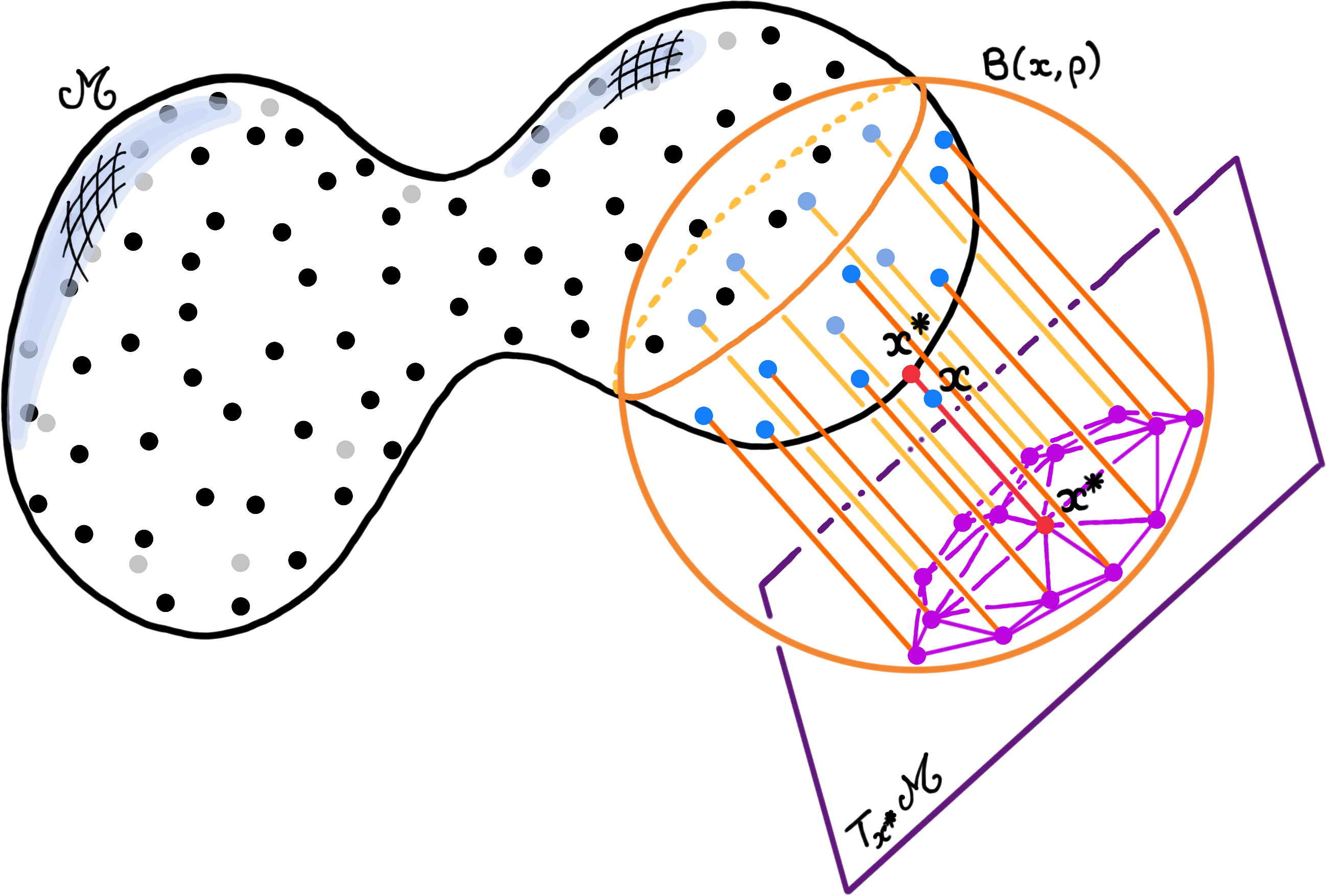
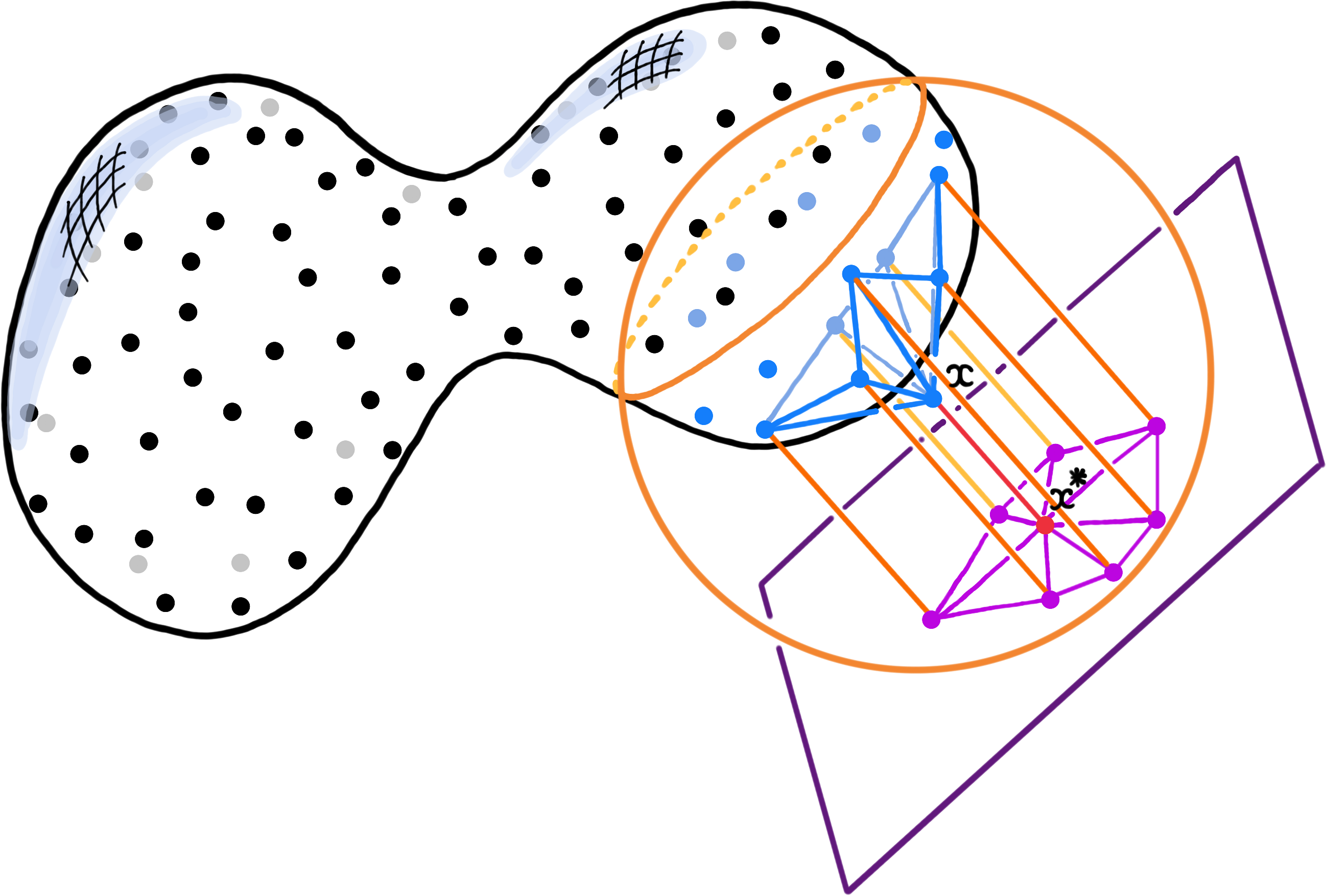
Figure 1: Construction of the prestar of $x$ at scale $\rho$. Left: Points in $P\cap B(x^{\ast},\rho)$ are projected onto the tangent space $\mathbf{T}_{x^{\ast}}\mathcal{M}$ and the Delaunay complex of the projected points is computed. For clarity, we have translated $\mathbf{T}_{x^{\ast}}\mathcal{M}$. Right: The star of $x^{\ast}$ (in purple) is the set of simplices that cover $x^{\ast}$ and the prestar of $x$ (in blue) is the set of simplices $\sigma\in P\cap B(x^{\ast},\rho)$ whose projection belongs to the star of $x^{\ast}$.

Definition 4 (Stars and Prestars).

Given a point $m\in\mathcal{M}$, we call the star of $m$ at scale $\rho$ the set of simplices

$$\operatorname{Star}_{P,\mathcal{M}}(m,\rho)=\{\tau\in\operatorname{Del}(\pi_{\mathbf{T}_{m}\mathcal{M}}(P\cap B(m,\rho)))\mid m\in\operatorname{conv}\tau\}.$$

Given a point $x\in\mathbb{R}^{N}\setminus\operatorname{axis}(\mathcal{M})$, we call the prestar of $x$ at scale $\rho$ the set of simplices

$$\begin{split}\operatorname{Prestar}_{P,\mathcal{M}}(x,\rho)=\{&\sigma\subseteq P\cap B(x^{*},\rho)\mid\pi_{\mathbf{T}_{x^{*}}\mathcal{M}}(\sigma)\in\operatorname{Star}_{P,\mathcal{M}}(x^{*},\rho)\}.\end{split}$$

Figure 1 illustrates the construction of the prestar of a point $x$ in $P$.

Remark 5.

By definition, if two points $x$ and $y$ share the same projection onto $\mathcal{M}$, that is, if $x^{*}=y^{*}$, then they also share the same prestar at scale $\rho$, that is, $\operatorname{Prestar}_{P,\mathcal{M}}(x,\rho)=\operatorname{Prestar}_{P,\mathcal{M}}(y,\rho)$. In particular, $\operatorname{Prestar}_{P,\mathcal{M}}(x,\rho)=\operatorname{Prestar}_{P,\mathcal{M}}(x^{*},\rho)$ whenever the projection at $x$ is well-defined.

Definition 6 (Flat Delaunay complex).

The flat Delaunay complex of $P$ with respect to $\mathcal{M}$ at scale $\rho$ is the set of simplices

$$\operatorname{FlatDel}_{\mathcal{M}}(P,\rho)=\bigcup_{p\in P}\operatorname{Prestar}_{P,\mathcal{M}}(p,\rho).$$

Note that the flat Delaunay complex is not necessarily a simplicial complex but becomes one under the assumptions of our two main theorems (Theorems 12 and 17).

3.2 Preliminary remarks

Remark 7.

By definition, if a simplex $\sigma$ belongs to the prestar of some point $x$ at scale $\rho$, then $\sigma$ fits in a ball of radius $\rho$ and therefore is $\rho$-small and so are simplices in $\operatorname{FlatDel}_{\mathcal{M}}(P,\rho)$.

Remark 8.

For all points $x$ at which $d(x,\mathcal{M})<\operatorname{reach}M$ and all $m\in\mathcal{M}$, we have that $m=\pi_{\mathbf{T}_{m}\mathcal{M}}(x)\iff m=\pi_{\mathcal{M}}(x)$.

We now provide two alternate characterizations of simplices in the prestar. The first one is a direct consequence of the above remark and will be useful in the proof of Theorem 17 and the second one will facilitate the proof of Lemma 37.

Remark 9 (First characterization of prestars).

If $x$ is a point at which $d(x,\mathcal{M})<\operatorname{reach}\mathcal{M}$ and $\rho<\operatorname{reach}\mathcal{M}$, then:

$$\sigma\in\operatorname{Prestar}_{P,\mathcal{M}}(x,\rho)~{}\iff~{}\begin{cases}\sigma\subseteq P\cap B(x^{*},\rho)\\ \pi_{\mathbf{T}_{x^{*}}\mathcal{M}}(\sigma)\in\operatorname{Del}(\pi_{\mathbf{T}_{x^{*}}\mathcal{M}}(P\cap B(x^{*},\rho)))\\ x^{*}\in\pi_{\mathcal{M}}(\operatorname{conv}\sigma)\end{cases}$$

Remark 10 (Second characterization of prestars).

For all simplices $\sigma$ such that $\operatorname{conv}\sigma\subseteq\mathcal{M}^{\oplus\rho}$ with $\rho<\operatorname{reach}\mathcal{M}$ and all $m\in\pi_{\mathcal{M}}(\operatorname{conv}\sigma)$,

$$\sigma\in\operatorname{Prestar}_{P,\mathcal{M}}(m,\rho)~{}\iff~{}\begin{cases}\sigma\subseteq P\cap B(m,\rho)\\ \pi_{\mathbf{T}_{m}\mathcal{M}}(\sigma)\in\operatorname{Del}(\pi_{\mathbf{T}_{m}\mathcal{M}}(P\cap B({m},\rho)))\end{cases}$$

Indeed, applying Remark 9 with $x=m$, we observe that the last condition on the right side of the equivalence is redundant because $m^{*}=m\in\pi_{\mathcal{M}}(\operatorname{conv}\sigma)$.

4 Faithful reconstruction from structural conditions

In this section, we exhibit a set of structural conditions under which $\operatorname{FlatDel}_{\mathcal{M}}(P,\rho)$ is a faithful reconstruction of $\mathcal{M}$. These conditions are encapsulated in our first reconstruction theorem (Theorem 12 below). Among the conditions, we find that every $\rho$-small $d$-simplex $\sigma\subseteq P$ must have its prestars in agreement at scale $\rho$:

Definition 11 (Prestars in agreement).

We say that the prestars of $\sigma$ are in agreement at scale $\rho$ if for all $x,y\in\operatorname{conv}\sigma$, the following equivalence holds: $\sigma\in\operatorname{Prestar}_{P,\mathcal{M}}(x,\rho)\iff\sigma\in\operatorname{Prestar}_{P,\mathcal{M}}(y,\rho)$.

Compare to the work in [7, 5], we define the prestars everywhere in space, not merely at the data points $P$ and we enforce the prestars to agree at every pair of points in $\operatorname{conv}\sigma$ and not merely at the vertices of $\sigma$. This trick allows us to provide a short proof that agreement of prestars, among other lighter conditions, imply that the flat Delaunay complex is a faithful reconstruction of $\mathcal{M}$.

Theorem 12 (Faithful reconstruction from structural conditions).

Suppose that $P\subseteq\mathcal{M}^{\oplus\rho}$ with $\rho<\frac{\mathcal{R}}{2}$ and assume that the following structural conditions are satisfied:

1. For every $\rho$-small $d$-simplex $\sigma\subseteq P$, the map ${\left.\kern-1.2pt\pi_{\mathcal{M}}\vphantom{\big{|}}\right|_{\operatorname{conv}\sigma}}$ is injective;

2. For all $m\in\mathcal{M}$, the map ${\left.\kern-1.2pt\pi_{\mathbf{T}_{m}\mathcal{M}}\vphantom{\big{|}}\right|_{P\cap B(m,\rho)}}$ is injective;

3. For all $m\in\mathcal{M}$, $\boldsymbol{\lvert}\operatorname{Star}_{P,\mathcal{M}}(m,\rho)\boldsymbol{\rvert}$ is homeomorphic to $\mathbb{R}^{d}$ in a neighborhood of $m$;

4. For all $m\in\mathcal{M}$, $\operatorname{Star}_{P,\mathcal{M}}(m,\rho)$ is geometrically realized;

5. Every $\rho$-small $d$-simplex $\sigma\subseteq P$ has its prestars in agreement at scale $\rho$.

Then,

• $\operatorname{FlatDel}_{\mathcal{M}}(P,\rho)$ is a simplicial complex;

• For all $m\in\mathcal{M}$, $\operatorname{Prestar}_{P,\mathcal{M}}(m,\rho)=\{\sigma\in\operatorname{FlatDel}_{\mathcal{M}}(P,\rho)\mid m\in\pi_{\mathcal{M}}(\operatorname{conv}\sigma)\}$;

• $\operatorname{FlatDel}_{\mathcal{M}}(P,\rho)$ is a faithful reconstruction of $\mathcal{M}$.

Before giving the proof, we start with a remark.

Remark 13.

For any simplex $\sigma\subseteq\mathcal{M}^{\oplus\rho}$ that can be enclosed in a ball of radius $\rho<\frac{\mathcal{R}}{2}$, then $\operatorname{conv}\sigma\subseteq\mathcal{M}^{\oplus 2\rho}$. Indeed, for all $x\in\operatorname{conv}\sigma$, $d(x,\mathcal{M})\leq d(x,\sigma)+\rho\leq 2\rho$. Hence, the map ${\left.\kern-1.2pt\pi_{\mathcal{M}}\vphantom{\big{|}}\right|_{\operatorname{conv}\sigma}}$ is well-defined.

Proof of Theorem 12.

We prove the lemma in seven (short) stages:

(a) First, we prove the following implication:

$$\begin{cases}\sigma\in\operatorname{Prestar}_{P,\mathcal{M}}(x,\rho)\\ \text{for all $x\in\operatorname{conv}\sigma$}\end{cases}\implies\quad\begin{cases}\tau\in\operatorname{Prestar}_{P,\mathcal{M}}(x,\rho)\\ \text{for all $\tau\subseteq\sigma$ and all $x\in\operatorname{conv}\tau$}\end{cases}$$

Indeed, suppose that $\sigma\in\operatorname{Prestar}_{P,\mathcal{M}}(x,\rho)$ for all $x\in\operatorname{conv}\sigma$. Using Remark 9, this is equivalent to saying that for all $x\in\operatorname{conv}\sigma$:

$$\begin{cases}\sigma\subseteq P\cap B(x^{*},\rho)\\ \pi_{\mathbf{T}_{x^{*}}\mathcal{M}}(\sigma)\in\operatorname{Del}(\pi_{\mathbf{T}_{x^{*}}\mathcal{M}}(P\cap B(x^{*},\rho)))\\ x^{*}\in\pi_{\mathcal{M}}(\operatorname{conv}\sigma)\end{cases}$$

Letting $x$ be any point of $\operatorname{conv}\tau$ and using $\tau\subseteq\sigma$, we obtain that:

$$\begin{cases}\tau\subseteq P\cap B(x^{*},\rho)\\ \pi_{\mathbf{T}_{x^{*}}\mathcal{M}}(\tau)\in\operatorname{Del}(\pi_{\mathbf{T}_{x^{*}}\mathcal{M}}(P\cap B(x^{*},\rho)))\\ x^{*}\in\pi_{\mathcal{M}}(\operatorname{conv}\tau)\end{cases}$$

But, using again Remark 9, this translates into saying that $\tau\in\operatorname{Prestar}_{P,\mathcal{M}}(x,\rho)$ for all $x\in\operatorname{conv}\tau$ as desired.

(b) Second, we establish the following implication:

$$\text{$\tau\in\operatorname{Prestar}_{P,\mathcal{M}}(m,\rho)$ for some $m\in\mathcal{M}$}\implies\text{$\tau\in\operatorname{Prestar}_{P,\mathcal{M}}(x,\rho)$ for all $x\in\operatorname{conv}\tau$}.$$

Consider a simplex $\tau\in\operatorname{Prestar}_{P,\mathcal{M}}(m,\rho)$ for some $m\in\mathcal{M}$ and let us show that $\tau\in\operatorname{Prestar}_{P,\mathcal{M}}(x,\rho)$ for all $x\in\operatorname{conv}\tau$. Since $\tau\in\operatorname{Prestar}_{P,\mathcal{M}}(m,\rho)$, this implies that $\tau^{\prime}=\pi_{\mathbf{T}_{m}\mathcal{M}}(\tau)\in\operatorname{Star}_{P,\mathcal{M}}(m,\rho)$. Because of hypothesis (3), $\boldsymbol{\lvert}\operatorname{Star}_{P,\mathcal{M}}(m,\rho)\boldsymbol{\rvert}$ is homeomorphic to $\mathbb{R}^{d}$ and therefore contains at least one $d$-simplex $\sigma^{\prime}\supseteq\tau^{\prime}$. Since $\sigma^{\prime}\in\operatorname{Star}_{P,\mathcal{M}}(m,\rho)$, it follows from the definition of the star that $\sigma^{\prime}\subseteq\pi_{\mathbf{T}_{m}\mathcal{M}}(P\cap B(m,\rho))$. Because of hypothesis (2), the projection $\pi_{\mathbf{T}_{m}\mathcal{M}}$ restricted to $P\cap B(m,\rho)$ is injective and therefore there exists a unique $\sigma\subseteq P\cap B(m,\rho)$ such that $\sigma^{\prime}=\pi_{\mathbf{T}_{m}\mathcal{M}}(\sigma)$ and furthermore $\sigma^{\prime}\supseteq\tau^{\prime}$ implies that $\sigma\supseteq\tau$. Since $\sigma\subseteq P\cap B(m,\rho)$ and $\sigma^{\prime}\in\operatorname{Star}_{P,\mathcal{M}}(m,\rho)$, we get that $\sigma\in\operatorname{Prestar}_{P,\mathcal{M}}(m,\rho)$. By hypothesis (5), the prestars of $\sigma$ are in agreement at scale $\rho$ and therefore $\sigma\in\operatorname{Prestar}_{P,\mathcal{M}}(m,\rho)$ implies $\sigma\in\operatorname{Prestar}_{P,\mathcal{M}}(x,\rho)$ for all $x\in\operatorname{conv}\sigma$. Using the previous stage, we get that $\tau\in\operatorname{Prestar}_{P,\mathcal{M}}(x,\rho)$ for all $x\in\operatorname{conv}\tau$ as desired.

(c) Third, we prove that $\operatorname{FlatDel}_{\mathcal{M}}(P,\rho)$ is a simplicial complex. Consider $\sigma\in\operatorname{FlatDel}_{\mathcal{M}}(P,\rho)$ and $\tau\subseteq\sigma$ and let us prove that $\tau\in\operatorname{FlatDel}_{\mathcal{M}}(P,\rho)$. By definition of the flat Delaunay complex, we can find $m\in\mathcal{M}$ such that $\sigma\in\operatorname{Prestar}_{P,\mathcal{M}}(m,\rho)$. Using Stage (b), we deduce that $\sigma\in\operatorname{Prestar}_{P,\mathcal{M}}(x,\rho)$ for all $x\in\operatorname{conv}\sigma$. Using Stage (a), $\tau\in\operatorname{Prestar}_{P,\mathcal{M}}(x,\rho)$ for all $x\in\operatorname{conv}\tau$. By picking $x\in\tau\subseteq P$, this shows that $\tau\in\operatorname{FlatDel}_{\mathcal{M}}(P,\rho)$.

(d) Fourth, we claim that

$$\operatorname{FlatDel}_{\mathcal{M}}(P,\rho)=\bigcup_{m\in\mathcal{M}}\operatorname{Prestar}_{P,\mathcal{M}}(m,\rho),$$ (1)

where the union is over all points $m$ of $\mathcal{M}$ and not merely points of $P$. The direct inclusion is clear. To establish the reverse inclusion, consider a simplex $\tau\in\operatorname{Prestar}_{P,\mathcal{M}}(m,\rho)$ for some $m\in\mathcal{M}$ and let us show that $\tau\in\operatorname{Prestar}_{P,\mathcal{M}}(p,\rho)$ for some $p\in P$. In Stage (b), we proved that $\tau\in\operatorname{Prestar}_{P,\mathcal{M}}(m,\rho)$ for some $m\in\mathcal{M}$ implies that $\tau\in\operatorname{Prestar}_{P,\mathcal{M}}(x,\rho)$ for all $x\in\operatorname{conv}\sigma$ and thus, picking $x$ among the vertices of $\tau$ establishes the claim.

(e) Fifth, we establish that for all $m\in\mathcal{M}$,

$$\operatorname{Prestar}_{P,\mathcal{M}}(m,\rho)=\{\sigma\in\operatorname{FlatDel}_{\mathcal{M}}(P,\rho)\mid m\in\pi_{\mathcal{M}}(\operatorname{conv}\sigma)\}.$$ (2)

Let $m\in\mathcal{M}$. To establish the direct inclusion, consider a simplex $\sigma\in\operatorname{Prestar}_{P,\mathcal{M}}(m,\rho)$. By Equation (1), $\sigma\in\operatorname{FlatDel}_{\mathcal{M}}(P,\rho)$, and by Remark 9, we get that $m\in\pi_{\mathcal{M}}(\operatorname{conv}\sigma)$. To establish the reverse inclusion, consider a simplex $\sigma\in\operatorname{FlatDel}_{\mathcal{M}}(P,\rho)$ such that $m\in\pi_{\mathcal{M}}(\operatorname{conv}\sigma)$. Because $\sigma\in\operatorname{FlatDel}_{\mathcal{M}}(P,\rho)$, we can find $m^{\prime}\in\mathcal{M}$ (which is the projection of a point of $P$) such that $\sigma\in\operatorname{Prestar}_{P,\mathcal{M}}(m^{\prime},\rho)$. Applying Stage (b), we deduce that $\sigma\in\operatorname{Prestar}_{P,\mathcal{M}}(m^{\prime},\rho)$ implies that $\sigma\in\operatorname{Prestar}_{P,\mathcal{M}}(x,\rho)$ for all $x\in\operatorname{conv}\sigma$ and picking $x\in\operatorname{conv}\sigma$ such that $m=\pi_{\mathcal{M}}(x)$ and using Remark 5, we deduce that $\sigma\in\operatorname{Prestar}_{P,\mathcal{M}}(m,\rho)$.

(f) Sixth, we prove that $\operatorname{FlatDel}_{\mathcal{M}}(P,\rho)$ is geometrically realized. Consider a pair $(\alpha,\beta)$ of simplices in $\operatorname{FlatDel}_{\mathcal{M}}(P,\rho)$ and let us prove that $\operatorname{conv}\alpha\cap\operatorname{conv}\beta=\operatorname{conv}(\alpha\cap\beta)$. Clearly, $\operatorname{conv}\alpha\cap\operatorname{conv}\beta\supseteq\operatorname{conv}(\alpha\cap\beta)$. To prove the converse inclusion, suppose that there exists a point $x\in\operatorname{conv}\alpha\cap\operatorname{conv}\beta$ and let us prove that $x\in\operatorname{conv}(\alpha\cap\beta)$. Because both $\alpha$ and $\beta$ are $\rho$-small, Remark 13 implies that $\pi_{\mathcal{M}}$ is well-defined on both and we write $m=\pi_{\mathcal{M}}(x)$. Because both $\alpha$ and $\beta$ belong to $\operatorname{FlatDel}_{\mathcal{M}}(P,\rho)$ while $\pi_{\mathcal{M}}(\operatorname{conv}\alpha)$ and $\pi_{\mathcal{M}}(\operatorname{conv}\beta)$ cover $m$, it follows from Equation (2) that both $\alpha$ and $\beta$ belong to $\operatorname{Prestar}_{P,\mathcal{M}}(m,\rho)$ and therefore both $\alpha^{\prime}=\pi_{\mathbf{T}_{m}\mathcal{M}}(\alpha)$ and $\beta^{\prime}=\pi_{\mathbf{T}_{m}\mathcal{M}}(\beta)$ belong to $\operatorname{Star}_{P,\mathcal{M}}(m,\rho)$. Since the latter is geometrically realized (hypothesis (4)), we have $m\in\operatorname{conv}\alpha^{\prime}\cap\operatorname{conv}\beta^{\prime}=\operatorname{conv}(\alpha^{\prime}\cap\beta^{\prime})$ and since we have assumed that the restrictiction of $\pi_{\mathbf{T}_{m}\mathcal{M}}$ to points in $P\cap B(m,\rho)\supseteq\alpha\cup\beta$ is injective, $m\in\operatorname{conv}(\alpha^{\prime}\cap\beta^{\prime})=\operatorname{conv}(\pi_{\mathbf{T}_{m}\mathcal{M}}(\alpha\cap\beta))=\pi_{\mathbf{T}_{m}\mathcal{M}}(\operatorname{conv}(\alpha\cap\beta))$. Using Remark 8, we get that $m=\pi_{\mathcal{M}}(x)=\pi_{\mathbf{T}_{m}\mathcal{M}}(x)$ and using the injectivity of $\pi_{\mathbf{T}_{m}\mathcal{M}}$ on $P\cap B(m,\rho)$, we get that $x\in\operatorname{conv}(\alpha\cap\beta)$. This proves that $\operatorname{FlatDel}_{\mathcal{M}}(P,\rho)$ is geometrically realized.

(g) Seventh, we prove that $\boldsymbol{\lvert}\operatorname{FlatDel}_{\mathcal{M}}(P,\rho)\boldsymbol{\rvert}$ is a $d$-manifold and that the map

$$\pi_{\mathcal{M}}:\boldsymbol{\lvert}\operatorname{FlatDel}_{\mathcal{M}}(P,\rho)\boldsymbol{\rvert}\to\mathcal{M}$$

is injective. Consider a point $x\in\boldsymbol{\lvert}\operatorname{FlatDel}_{\mathcal{M}}(P,\rho)\boldsymbol{\rvert}$ and let $m=\pi_{\mathcal{M}}(x)$. Observe that in a small neighborhood of $x$, the set $\boldsymbol{\lvert}\operatorname{FlatDel}_{\mathcal{M}}(P,\rho)\boldsymbol{\rvert}$ coincides with the set $\boldsymbol{\lvert}\operatorname{Prestar}_{P,\mathcal{M}}(m,\rho)\boldsymbol{\rvert}$ because of Equation (2). Note that the map $\pi_{\mathbf{T}_{m}\mathcal{M}}$ is a bijective correspondence between $P\cap B(m,\rho)$ and $\pi_{\mathbf{T}_{m}\mathcal{M}}(P\cap B(m,\rho))$ such that $\sigma\in\operatorname{Prestar}_{P,\mathcal{M}}(m,\rho)$ if and only if $\pi_{\mathbf{T}_{m}\mathcal{M}}(\sigma)\in\operatorname{Star}_{P,\mathcal{M}}(m,\rho)$. We note that $\sigma$ and $\pi_{\mathbf{T}_{m}\mathcal{M}}(\sigma)$ which share the same dimension are both non-degenerate. Indeed, $\pi_{\mathbf{T}_{m}\mathcal{M}}(\sigma)$ is non-degenerate because it belongs to $\operatorname{Star}_{P,\mathcal{M}}(m,\rho)$ which we have assumed to be geometrically realized (hypothesis (4)). Simplex $\sigma$ is also non-degenerate since $\sigma$ has as many vertices as $\pi_{\mathbf{T}_{m}\mathcal{M}}(\sigma)$ and the dimension of $\operatorname{aff}\sigma$ cannot be smaller than the dimension of its projection $\operatorname{aff}\pi_{\mathbf{T}_{m}\mathcal{M}}(\sigma)$ which is full. Hence, $\pi_{\mathbf{T}_{m}\mathcal{M}}$ is an isomorphism between $\operatorname{Prestar}_{P,\mathcal{M}}(m,\rho)$ and $\operatorname{Star}_{P,\mathcal{M}}(m,\rho)$ and both $\operatorname{Prestar}_{P,\mathcal{M}}(m,\rho)$ and $\operatorname{Star}_{P,\mathcal{M}}(m,\rho)$ are geometrically realized. We deduce that the induced simplicial map $\pi_{\mathbf{T}_{m}\mathcal{M}}:\boldsymbol{\lvert}\operatorname{Prestar}_{P,\mathcal{M}}(m,\rho)\boldsymbol{\rvert}\to\boldsymbol{\lvert}\operatorname{Star}_{P,\mathcal{M}}(m,\rho)\boldsymbol{\rvert}$ is a homeomorphism. Since in a neighborhood of $m$, $\boldsymbol{\lvert}\operatorname{Star}_{P,\mathcal{M}}(m,\rho)\boldsymbol{\rvert}$ is homeomorphic to $\mathbb{R}^{d}$, it follows that in a neighborhood of $x$, $\boldsymbol{\lvert}\operatorname{FlatDel}_{\mathcal{M}}(P,\rho)\boldsymbol{\rvert}$ which coincides with $\boldsymbol{\lvert}\operatorname{Prestar}_{P,\mathcal{M}}(m,\rho)\boldsymbol{\rvert}$ is also homeomorphic to $\mathbb{R}^{d}$. This proves that $\boldsymbol{\lvert}\operatorname{FlatDel}_{\mathcal{M}}(P,\rho)\boldsymbol{\rvert}$ is a $d$-manifold. Let us prove that $\pi_{\mathcal{M}}:\boldsymbol{\lvert}\operatorname{FlatDel}_{\mathcal{M}}(P,\rho)\boldsymbol{\rvert}\to\mathcal{M}$ is injective. Consider two points $x$ and $y$ in $\boldsymbol{\lvert}\operatorname{FlatDel}_{\mathcal{M}}(P,\rho)\boldsymbol{\rvert}$ such that $\pi_{\mathcal{M}}(x)=\pi_{\mathcal{M}}(y)=m$. Then, by Remark 8, $\pi_{\mathbf{T}_{m}\mathcal{M}}(x)=\pi_{\mathbf{T}_{m}\mathcal{M}}(y)=m$ and since we have just established that $\pi_{\mathbf{T}_{m}\mathcal{M}}:\boldsymbol{\lvert}\operatorname{Prestar}_{P,\mathcal{M}}(m,\rho)\boldsymbol{\rvert}\to\boldsymbol{\lvert}\operatorname{Star}_{P,\mathcal{M}}(m,\rho)\boldsymbol{\rvert}$ is a homeomorphism, we deduce that $x=y$, establishing the injectivity of $\pi_{\mathcal{M}}$.

(h) Finally, we prove that $\pi_{\mathcal{M}}$ is a homeomorphism between $\mathcal{D}=\boldsymbol{\lvert}\operatorname{FlatDel}_{\mathcal{M}}(P,\rho)\boldsymbol{\rvert}$ and $\mathcal{M}$. Recall that $\mathcal{D}$ and $\mathcal{M}$ are two $d$-manifolds (without boundary) and that the restriction of $\pi_{\mathcal{M}}$ to $\mathcal{D}$ is an injective continuous map. Since for all $m\in\mathcal{M}$, $\boldsymbol{\lvert}\operatorname{Star}_{P,\mathcal{M}}(m,\rho)\boldsymbol{\rvert}$ is homeomorphic to $\mathbb{R}^{d}$ in a neighborhood of $m$, this implies that there exists $x\in\mathcal{D}$ such that $\pi_{\mathcal{M}}(x)=m$ and ${\left.\kern-1.2pt\pi_{\mathcal{M}}\vphantom{\big{|}}\right|_{\mathcal{D}}}$ is surjective. Applying the domain invariance theorem, we get that $\pi_{\mathcal{M}}:\mathcal{D}\to\mathcal{M}$ is open and therefore $\pi_{\mathcal{M}}$ is a homeomorphism between $\mathcal{D}$ and $\pi_{\mathcal{M}}(\mathcal{D})=\mathcal{M}$. ∎

5 Faithful reconstruction from sampling and safety conditions

In this section, we state our second reconstruction theorem (Theorem 17 below). The theorem describes geometric conditions on $P$ under which (1) $\operatorname{FlatDel}_{\mathcal{M}}(P,\rho)$ is a faithful reconstruction of $\mathcal{M}$ and (2) $\operatorname{FlatDel}_{\mathcal{M}}(P,\rho)$ satisfies certain properties that are needed in our companion paper [4]. In particular, the theorem provides a characterization of $d$-simplices in $\operatorname{FlatDel}_{\mathcal{M}}(P,\rho)$ as the $d$-simplices that are delloc in $P$ at scale $\rho$:

Definition 14 (Delloc simplex).

We say that a simplex $\sigma$ is delloc in $P$ at scale $\rho$ if $\sigma\in\operatorname{Del}(\pi_{\operatorname{aff}\sigma}(P\cap B(c_{\sigma},\rho))$.

Note that deciding whether a simplex is delloc does not require the knowledge of the manifold $\mathcal{M}$. We emphasize the fact that the characterization of $d$-simplices in the flat Delaunay complex as the one being delloc turns out to be crucial in our companion paper [4].

In this section, we first introduce the necessary notations and definitions to describe the geometric conditions on $P$ that we need. We then state our second reconstruction theorem and sketch the proof.

Definition 15 (Dense, accurate, and separated).

We say that $P$ is an $\varepsilon$-dense sample of $\mathcal{M}$ if for every point $m\in\mathcal{M}$, there is a point $p\in P$ with $\|p-m\|\leq\varepsilon$ or, equivalently, if $\mathcal{M}\subseteq P^{\oplus\varepsilon}$. We say that $P$ is a $\delta$-accurate sample of $\mathcal{M}$ if for every point $p\in P$, there is a point $m\in\mathcal{M}$ with $\|p-m\|\leq\delta$ or, equivalently, if $P\subseteq\mathcal{M}^{\oplus\delta}$. Let $\operatorname{separation}(P)=\min_{p,q\in P}\|p-q\|$.

We stress that our definition of a protected simplex differs slightly from the one in [8, 7].

Definition 16 (Protection).

We say that a non-degenerate simplex $\sigma\subseteq\mathbb{R}^{N}$ is $\zeta$-protected with respect to $Q\subseteq\mathbb{R}^{N}$ if for all $q\in Q\setminus\sigma$, we have $d(q,S(\sigma))>\zeta$. We shall simply say that $\sigma$ is protected with respect to $Q$ when it is $0$-protected with respect to $Q$.

Let $\mathcal{H}(\sigma)=\{\mathbf{T}_{m}\mathcal{M}\mid m\in\pi_{\mathcal{M}}(\operatorname{conv}\sigma)\}\cup\{\operatorname{aff}\sigma\}$, and $\Theta(\sigma)=\max_{H_{0},H_{1}\in\mathcal{H}(\sigma)}\angle(H_{0},H_{1})$. To the pair $(P,\rho)$ we now associate three quantities that describe the quality of $P$ at scale $\rho$:

• $\operatorname{height}(P,\rho)=\min_{\sigma}0pt{\sigma}$, where the minimum is over all $\rho$-small $d$-simplices $\sigma\subseteq P$;

• $\Theta(P,\rho)=\max_{\sigma}\Theta(\sigma)$, where $\sigma$ ranges over all $\rho$-small $d$-simplices of $P$;

• $\operatorname{protection}(P,\rho)=\min_{\sigma}\min_{q}d(q,S(\sigma))$, where the minima are over all $\rho$-small $d$-simplices $\sigma\subseteq P$ and all points $q\in\pi_{\operatorname{aff}\sigma}(P\cap B(c_{\sigma},\rho))\setminus\sigma$.

Theorem 17 (Faithful reconstruction from sampling and safety conditions).

Let $\varepsilon$, $\delta$, $\rho$, $\theta$ be non-negative real numbers and set $A=4\delta\theta+4\rho\theta^{2}$. Assume that $\theta\leq\frac{\pi}{6}$, $\delta\leq\varepsilon$, and $16\varepsilon\leq\rho<\frac{\mathcal{R}}{4}$. Suppose that $P$ satisfies the following sampling conditions: $P$ is a $\delta$-accurate $\varepsilon$-dense sample of $\mathcal{M}$. Suppose furthermore that $P$ satisfies the following safety conditions:

1. $\Theta(P,\rho)\leq\theta-2\arcsin\left(\frac{\rho+\delta}{\mathcal{R}}\right)$.

2. $\operatorname{separation}(P)>2A+6\delta+\frac{2\rho^{2}}{\mathcal{R}}$;

3. $\operatorname{height}(P,\rho)>0$ and $\operatorname{protection}(P,3\rho)>2A\left(1+\frac{4d\varepsilon}{\operatorname{height}(P,\rho)}\right)$.

Then we have the following properties:

Faithful reconstruction:

$\operatorname{FlatDel}_{\mathcal{M}}(P,\rho)$ is a faithful reconstruction of $\mathcal{M}$;

Prestar formula:

$\operatorname{Prestar}_{P,\mathcal{M}}(m,\rho)=\{\sigma\in\operatorname{FlatDel}_{\mathcal{M}}(P,\rho)\mid m\in\pi_{\mathcal{M}}(\operatorname{conv}\sigma)\},\;\forall m\in\mathcal{M}$;

Circumradii:

For all $d$-simplices $\sigma\in\operatorname{FlatDel}_{\mathcal{M}}(P,\rho)$, we have that $R(\sigma)\leq\varepsilon$;

Characterization:

For all $d$-simplices $\sigma$, $\sigma\in{\operatorname{FlatDel}_{\mathcal{M}}(P,\rho)}\iff\sigma$ delloc in $P$ at scale $\rho$.

The geometric conditions that we need for our result can be divided in two groups: the sampling conditions and the safety conditions. Roughly speaking, the sampling conditions say that $P$ must be “sufficiently” dense and “sufficiently” accurate. The safety conditions say that (1) the angle that $\rho$-small $d$-simplices make with “nearby” tangent space to $\mathcal{M}$ must be sufficiently small; (2) points in $P$ must be “sufficiently” well separated; (3) both the protection and the height of $P$ at scale $\rho$ must be “sufficiently” lower bounded. Whereas it seems reasonable to assume that $P$ satisfies the samping conditions, it is less clear that, in practice, $P$ can satisfy both the sampling and safety conditions. We show in Section 9 that starting from a situation where $P$ satisfies some “strong” sampling conditions, it is always possible to perturb $P$ in such a way that after perturbation, $P$ satisfies both the sampling and safety conditions of Theorem 17.

Before sketching the proof of our second theorem, we derive a corollary that may have computational implications in low-dimensional ambient spaces. For this, we recall that $\sigma$ is a Gabriel simplex of $P$ if its smallest circumsphere $S(\sigma)$ does not enclose any point of $P$ in its interior.

Corollary 18.

Under the assumptions of Theorem 17, the $d$-simplices of $\operatorname{FlatDel}_{\mathcal{M}}(P,\rho)$ are Gabriel simplices and therefore $\operatorname{FlatDel}_{\mathcal{M}}(P,\rho)\subseteq\operatorname{Del}(P)$.

Proof.

It is easy to see that a delloc simplex $\sigma$ in $P$ at scale $\rho$ is also a Gabriel simplex of $P$ whenever $2R(\sigma)\leq\rho$. The result follows because under the assumption of Theorem 17, $d$-simplices of $\operatorname{FlatDel}_{\mathcal{M}}(P,\rho)$ are delloc in $P$ at scale $\rho$. ∎

Sketch of the proof.

The proof consists in showing that the sampling and safety conditions of Theorem 17 imply the structural conditions of Theorem 12. Applying Theorem 12, we then get that, amongst other properties, $\operatorname{FlatDel}_{\mathcal{M}}(P,\rho)$ is a faithful reconstruction of $\mathcal{M}$. It is not too difficult to show that the sampling and safety conditions of Theorem 17 imply the first three structural conditions of Theorem 12. This will be established in Section 6. The tricky part consists in proving that the sampling and safety conditions imply the last two structural conditions, and in particular imply that every $\rho$-small $d$-simplex $\sigma\subseteq P$ has its prestarts in agreement at scale $\rho$. Let us introduce the following definitions:

Definition 19 (Delaunay stability at scale $\rho$).

Let $\{(h_{i},H_{i})\}_{i\in I}$ be a (possibly infinite) set, where $h_{i}$ designates a point of $\mathbb{R}^{N}$ and $H_{i}\subseteq\mathbb{R}^{N}$ designates a $d$-dimensional affine space. We say that $\sigma$ is Delaunay stable for $P$ at scale $\rho$ with respect to the set $\{(h_{i},H_{i})\}_{i\in I}$ if the following two propositions are equivalent for all $a,b\in I$:

• $\sigma\subseteq P\cap B(h_{a},\rho)$ and $\pi_{H_{a}}(\sigma)\in\operatorname{Del}(\pi_{H_{a}}(P\cap B(h_{a},\rho)))$;

• $\sigma\subseteq P\cap B(h_{b},\rho)$ and $\pi_{H_{b}}(\sigma)\in\operatorname{Del}(\pi_{H_{b}}(P\cap B(h_{b},\rho)))$.

Definition 20 (Standard neighborhood).

We define the standard neighborhood of $\sigma$ as the set $\mathscr{H}(\sigma)=\{(c_{\sigma},\operatorname{aff}\sigma)\}\cup\{(x^{\ast},\mathbf{T}_{x^{\ast}}\mathcal{M})\}_{x\in\operatorname{conv}\sigma}.$

Roughly speaking, the next lemma tells us that the Delaunay stability of a $\rho$-small $d$-simplex $\sigma$ with respect to its standard neighborhood $\mathscr{H}(\sigma)$ implies both agreement of prestars of $\sigma$ and a characterization of the property for $\sigma$ to belong to $\operatorname{FlatDel}_{\mathcal{M}}(P,\rho)$ in terms of being delloc. Precisely:

Lemma 21.

Suppose that $P\subseteq\mathcal{M}^{\oplus\rho}$ with $\rho<\mathcal{R}$ and that for all $m\in\mathcal{M}$, the restriction of map $\pi_{\mathbf{T}_{m}\mathcal{M}}$ to $P\cap B(m,\rho)$ is injective. Consider a $\rho$-small $d$-simplex $\sigma\subseteq P$ and suppose that $\sigma$ is Delaunay stable for $P$ at scale $\rho$ with respect to its standard neighborhood. Then,

• the prestars of $\sigma$ are in agreement at scale $\rho$;

• $\sigma\in\operatorname{FlatDel}_{\mathcal{M}}(P,\rho)\iff$ $\sigma$ is delloc in $P$ at scale $\rho$.

Proof.

Consider the following two propositions:

(a)

$\sigma\subseteq P\cap B(c_{\sigma},\rho)$ and $\sigma\in\operatorname{Del}(\pi_{\operatorname{aff}\sigma}(P\cap B(c_{\sigma},\rho)))$;

(b_x)

$\sigma\subseteq P\cap B(x^{\ast},\rho)$ and $\pi_{\mathbf{T}_{x^{\ast}}\mathcal{M}}(\sigma)\in\operatorname{Del}(\pi_{\mathbf{T}_{x^{\ast}}\mathcal{M}}(P\cap B({x^{\ast}},\rho)))$.

Our Delaunay stability hypothesis is equivalent to saying that for all $x\in\operatorname{conv}\sigma$, we have (a) $\iff$ (b_x) and for all $x,y\in\operatorname{conv}\sigma$, we have (b_x) $\iff$ (b_y). Using Definition 14 and Remark 10, we can rewrite Propositions (a) and (b_x) respectively as:

(a)

$\sigma\text{ delloc in $P$ at scale $\rho$}$;

(b_x)

$\sigma\in\operatorname{Prestar}_{P,\mathcal{M}}(x,\rho)$.

Since (b_x) $\iff$ (b_y) for all $x,y\in\operatorname{conv}\sigma$, we get that $\sigma\in\operatorname{Prestar}_{P,\mathcal{M}}(x,\rho)$ $\iff$ $\sigma\in\operatorname{Prestar}_{P,\mathcal{M}}(y,\rho)$ for all $x,y\in\operatorname{conv}\sigma$. In other words, the prestars of $\sigma$ are in agreement and the first item of the lemma holds.

To see that we get the second item of the lemma as well, we claim that $\sigma\in\operatorname{FlatDel}_{\mathcal{M}}(P,\rho)$ $\iff$ there exists $v\in\sigma$ such that $\sigma\in\operatorname{Prestar}_{P,\mathcal{M}}(v,\rho)$. The reverse inclusion is clear. To get the direct inclusion, consider $v\in P$ such that $\sigma\in\operatorname{Prestar}_{P,\mathcal{M}}(v,\rho)$ and let us prove that $v\in\sigma$. Because $P\subseteq\mathcal{M}^{\oplus\rho}$ for $\rho<\mathcal{R}$, $\pi_{\mathcal{M}}$ is well-defined at $v$ and letting $v^{\ast}=\pi_{\mathcal{M}}(v)$, we clearly have $v\in P\cap B(v^{\ast},\rho)$. It follows from our definition of a prestar that

$$\sigma\in\operatorname{Prestar}_{P,\mathcal{M}}(v,\rho)~{}\iff~{}\begin{cases}\sigma\subseteq P\cap B(v^{\ast},\rho)\\ \pi_{\mathbf{T}_{v^{\ast}}\mathcal{M}}(\sigma)\in\operatorname{Del}(\pi_{\mathbf{T}_{v^{\ast}}\mathcal{M}}(P\cap B(v^{\ast},\rho)))\\ v^{\ast}\in\pi_{\mathbf{T}_{v^{\ast}}\mathcal{M}}(\operatorname{conv}\sigma)\end{cases}$$

By Remark 8, $v^{\ast}=\pi_{\mathcal{M}}(v)=\pi_{\mathbf{T}_{v^{\ast}}\mathcal{M}}(v)$ and therefore $\pi_{\mathbf{T}_{v^{\ast}}\mathcal{M}}(v)\in\operatorname{conv}(\pi_{\mathbf{T}_{v^{\ast}}\mathcal{M}}(\sigma))$. Since $\pi_{\mathbf{T}_{v^{\ast}}\mathcal{M}}(\sigma)\in\operatorname{Del}(\pi_{\mathbf{T}_{v^{\ast}}\mathcal{M}}(P\cap B(v^{\ast},\rho)))$, the only possibility is that $\pi_{\mathbf{T}_{v^{\ast}}\mathcal{M}}(v)\in\pi_{\mathbf{T}_{v^{\ast}}\mathcal{M}}(\sigma)$ and since $\pi_{\mathbf{T}_{v^{\ast}}\mathcal{M}}$ is injective on $P\cap B(v^{\ast},\rho)$ (by hypothesis), it follows that $v\in\sigma$ as claimed. Hence, we have just proved that $\sigma\in\operatorname{FlatDel}_{\mathcal{M}}(P,\rho)$ $\iff$ there exists $v\in\sigma$ such that (b_v). Since the latter is equivalent to (a) by hypothesis and (a) can be rewritten as $\sigma$ is delloc in $P$ at scale $\rho$, we get the secend item of the lemma. ∎

The above lemma suggests that we need first to establish the Delaunay stability of $\rho$-small $d$-simplices with respect to their standard neighborhood. We proceed in three steps. In Section 6, we enunciate basic properties on projection maps. We also establish geometric conditions under which the first three structural conditions of Theorem 12 hold. In Section 7, we study the Delaunay stability of $d$-simplices with respect to a general set $\{(h_{0},H_{0}),(h_{1},H_{1})\}$, where each pair $(h_{i},H_{i})$ consists of a point $h_{i}$ and a $d$-dimensional affine space $H_{i}$ through $h_{i}$. In Section 8, we prove our second theorem by first establishing the Delaunay stability of $d$-simplices with respect to their standard neighborhood.

6 Basic properties on projection maps

In this section, we enunciate basic properties on projection maps that we need for the proof of Theorem 17. We also establish geometric conditions under which the first three structural conditions of Theorem 12 hold. Those conditions are described respectively in Lemma 22, Lemma 23 and Lemma 26.

Lemma 22 (Injectivity of ${\left.\kern-1.2pt\pi_{\mathcal{M}}\vphantom{\big{|}}\right|_{\operatorname{conv}\sigma}}$).

Consider $\sigma\subseteq\mathbb{R}^{N}$ such that $\operatorname{conv}\sigma\subseteq\mathbb{R}^{N}\setminus\operatorname{axis}(\mathcal{M})$. If $\Theta(\sigma)<\frac{\pi}{2}$, then ${\left.\kern-1.2pt\pi_{\mathcal{M}}\vphantom{\big{|}}\right|_{\operatorname{conv}\sigma}}$ is injective.

Proof.

Suppose for a contradiction that there exist two points $x\neq y$ in $\operatorname{conv}\sigma$ that share the same projection $m$ onto $\mathcal{M}$, in other words, such that $x^{\ast}=y^{\ast}=m$. Then, the straight-line passing through $x$ and $y$ would be orthogonal to the tangent space $\mathbf{T}_{m}\mathcal{M}$, implying that $\angle(\mathbf{T}_{m}\mathcal{M},\operatorname{conv}\sigma)=\frac{\pi}{2}$ and therefore $\Theta(\sigma)=\max_{H_{0},H_{1}\in\mathcal{H}(\sigma)}\angle(H_{0},H_{1})=\frac{\pi}{2}$. But this contradicts our assumption that $\Theta(\sigma)<\frac{\pi}{2}$. ∎

Lemma 23 (Injectivity of ${\left.\kern-1.2pt\pi_{\mathbf{T}_{m}\mathcal{M}}\vphantom{\big{|}}\right|_{P\cap B(m,\rho)}}$).

Suppose that $P\subseteq\mathcal{M}^{\oplus\delta}$ with $16\delta\leq\rho\leq\frac{\mathcal{R}}{3}$ and $\operatorname{separation}(P)>\frac{2\rho^{2}}{\mathcal{R}}+2\delta$. Then, ${\left.\kern-1.2pt\pi_{\mathbf{T}_{m}\mathcal{M}}\vphantom{\big{|}}\right|_{P\cap B(m,\rho)}}$ is injective for all $m\in\mathcal{M}$.

Proof.

Consider two points $a,b\in P\cap B(m,\rho)$ and let $\theta=\angle(\mathbf{T}_{m}\mathcal{M},ab)$. We have $\cos\theta\times\|a-b\|\leq\|\pi_{\mathbf{T}_{m}\mathcal{M}}(a)-\pi_{\mathbf{T}_{m}\mathcal{M}}(b)\|$, showing that the restriction of $\pi_{\mathbf{T}_{m}\mathcal{M}}$ to $B(m,\rho)$ is injective as soon as $\theta<\frac{\pi}{2}$. Applying Lemma 44 with $\tau=\{a,b\}$ and $z=m$, we obtain that $\theta$ is upper bounded by

$$\theta\leq\arcsin\left(\frac{2}{\|a-b\|}\left(\frac{\rho^{2}}{\mathcal{R}}+\delta\right)\right)\leq\arcsin\left(\frac{2}{\operatorname{separation}(P)}\left(\frac{\rho^{2}}{\mathcal{R}}+\delta\right)\right)$$

and thus becomes smaller than $\frac{\pi}{2}$ for $\operatorname{separation}(P)>\frac{2\rho^{2}}{\mathcal{R}}+2\delta$. ∎

Lemma 24 (Local surjectivity of $\pi_{H}$).

Suppose $\rho<\frac{\mathcal{R}}{3}$. Let $H\subseteq\mathbb{R}^{N}$ be a $d$-dimensional affine space. Suppose that $H$ passes through a point $h$ such that $d(h,\mathcal{M})\leq\frac{\rho}{4}$ and that there exists $\theta\leq\frac{\pi}{6}$ such that $\angle(H,\mathbf{T}_{\pi_{\mathcal{M}}(h)}\mathcal{M})+2\arcsin\frac{\rho}{\mathcal{R}}\leq\theta$. Then,

$$H\cap B(h,\frac{\rho}{4})~{}\subseteq~{}\pi_{H}(\mathcal{M}\cap B(h,\frac{3\rho}{4})).$$

Proof.

Write $U=\mathcal{M}\cap B(h,\frac{3\rho}{4})$ and $V=H\cap B(h,\frac{\rho}{4})$; see Figure 2, right. We need to prove that $V\subseteq\pi_{H}(U)$. We start by establishing the following three propositions:

1. $\pi_{H}$ is a homeomorphism from $\mathcal{M}\cap B(h,\rho)$ to $\pi_{H}(\mathcal{M}\cap B(h,\rho))$;

2. $\partial\pi_{H}(U)\cap V=\emptyset$;

3. $\pi_{H}(U)\cap V\neq\emptyset$.

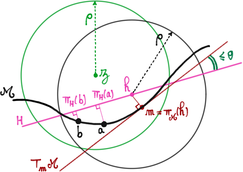
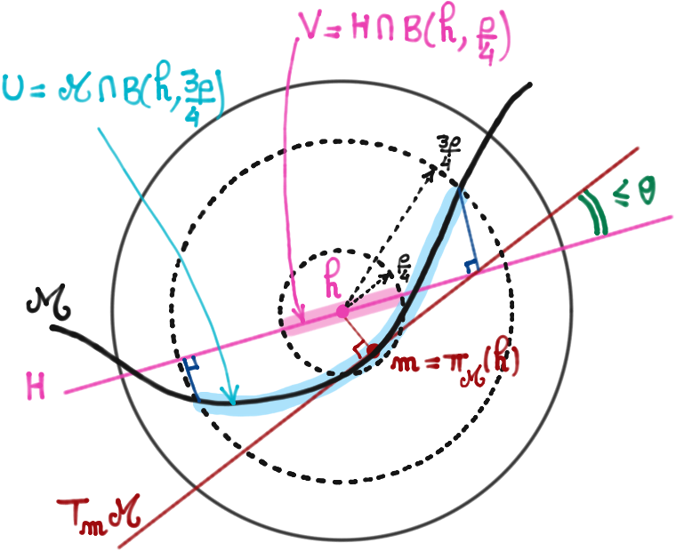
Figure 2: Notations for the proof of Lemma 24.

Let us prove Proposition (a). For all $a,b\in\mathcal{M}\cap B(h,\rho)$, we start by bounding $\angle(H,ab)$. Letting $h^{\ast}=\pi_{\mathcal{M}}(h)$ and using Lemma 41 and Lemma 42, we obtain

$$\angle(H,ab) \leq \angle(H,\mathbf{T}_{{h^{\ast}}}\mathcal{M})+\angle(\mathbf{T}_{{h^{\ast}}}\mathcal{M},\mathbf{T}_{a}\mathcal{M})+\angle(\mathbf{T}_{a}\mathcal{M},ab)$$

$$\leq \angle(H,\mathbf{T}_{{h^{\ast}}}\mathcal{M})+2\arcsin\left(\frac{\|a-{h^{\ast}}\|}{2\mathcal{R}}\right)+\arcsin\left(\frac{\|a-b\|}{2\mathcal{R}}\right)$$

$$\leq \angle(H,\mathbf{T}_{h^{\ast}}\mathcal{M})+\arcsin\left(\frac{\|a-h\|+\|h-h^{\ast}\|}{\mathcal{R}}\right)+\arcsin\frac{\rho}{\mathcal{R}}$$

$$\leq \angle(H,\mathbf{T}_{h^{\ast}}\mathcal{M})+\arcsin\left(\frac{\rho+\frac{\rho}{4}}{\mathcal{R}}\right)+\arcsin\frac{\rho}{\mathcal{R}}$$

$$\leq \angle(H,\mathbf{T}_{h^{\ast}}\mathcal{M})+2\arcsin\frac{\rho}{\mathcal{R}}$$

$$\leq \theta.$$

Hence, for all $a,b\in\mathcal{M}\cap B(h,\rho)$:

$$\cos\theta\times\|b-a\|~{}~{}\leq~{}~{}\cos\angle(H,ab)\times\|b-a\|=\|\pi_{H}(b)-\pi_{H}(a)\|~{}~{}\leq~{}~{}\|b-a\|,$$ (3)

showing that the restriction of $\pi_{H}$ to $\mathcal{M}\cap B(h,\rho)$ is injective as soon as $\theta<\frac{\pi}{2}$. Thus, $\pi_{H}$ is a homeomorphism from $\mathcal{M}\cap B(z,\rho)$ to its range $\pi_{H}(\mathcal{M}\cap B(z,\rho))$.

Let us prove Proposition (b). Because $\mathcal{M}\cap B(h,\rho)$ and $\pi_{H}(\mathcal{M}\cap B(h,\rho))$ are homeomorphic, we get in particular that $\partial\pi_{H}(U)=\pi_{H}(\partial U)$. Consider a point $u\in\partial U$, that is, a point $u\in\mathcal{M}$ such that $\|u-h\|=\frac{3\rho}{4}$ and let us prove that $\|\pi_{H}(u)-h\|>\frac{\rho}{4}$, in other words, that $\pi_{H}(u)$ not in $V$. By construction, both $u$ and $m=\pi_{\mathcal{M}}(h)$ belong to $\mathcal{M}\cap B(h,\rho)$ and thus $\angle(H,um)\leq\theta$. Using Equation (3) with $a=u$ and $b=m$, we get that $\|\pi_{H}(u)-\pi_{H}(m)\|\geq\cos\theta\times\|u-m\|$. We consider two cases:

• If $m=h$, we deduce immediately that $\|\pi_{H}(u)-h\|\geq\cos\theta\times\|u-h\|\geq\cos\frac{\pi}{6}\times\frac{3\rho}{4}>\frac{\rho}{4}$.

• If $m\neq h$, we claim that $\|\pi_{H}(u)-h\|>\frac{\rho}{4}$. To see this, denote by $\operatorname{Vec}(A)$ the vector space associated to an affine space $A$ and let $V^{\perp}$ designate the vector space orthogonal to a vector space $V$. Consider the straight-line $mh$ passing through $m$ and $h$. Note that $\pi_{H}(m)$ is also the orthogonal projection of $h$ onto the affine space orthogonal to $H$ and passing through $m$. It follows that the vector $\pi_{H}(m)-m$ is the orthogonal projection onto $\operatorname{Vec}(H)^{\perp}$ of the vector $h-m\in\operatorname{Vec}(\mathbf{T}_{m}\mathcal{M})^{\perp}$, so that $\angle(m\pi_{H}(m),mh)\leq\angle(\operatorname{Vec}(H)^{\perp},\operatorname{Vec}(\mathbf{T}_{m}\mathcal{M})^{\perp})=\angle(H,\mathbf{T}_{m}\mathcal{M})\leq\theta$. We thus get

  $$\|\pi_{H}(u)-h\| \geq\|\pi_{H}(u)-\pi_{H}(m)\|-\|h-\pi_{H}(m)\|$$

  $$\geq\cos\theta\times\|u-m\|-\sin\theta\times\|h-m\|$$

  $$\geq\cos\theta\times\left(\|u-h\|-\|m-h\|\right)-\sin\theta\times\|m-h\|$$

  $$\geq\cos\theta\times\frac{3\rho}{4}-(\cos\theta+\sin\theta)\times\frac{\rho}{4}$$

  $$\geq(2\cos\frac{\pi}{6}-\sin\frac{\pi}{6})\times\frac{\rho}{4}$$

  $$>\frac{\rho}{4}.$$

Let us prove Proposition (c) by showing that $\pi_{H}(m)\in\pi_{H}(U)\cap V$. First, we show that $m\in U=\mathcal{M}\cap B(h,\frac{3\rho}{4})$. Because $\|h-m\|=d(h,\mathcal{M})\leq\frac{\rho}{4}$, clearly $m\in\mathcal{M}\cap B(h,\frac{\rho}{4})\subseteq U$. Second, we show that $\pi_{H}(m)\in V=H\cap B(h,\frac{\rho}{4})$. Since triangle $mh\pi_{H}(m)$ has a right angle at vertex $\pi_{H}(m)$, the distance between any pair of points in this triangle is upper bounded by the lenght of its hypothenuse $mh$ and therefore, $\|h-\pi_{H}(m)\|\leq\|m-h\|\leq\frac{\rho}{4}$. Hence, $\pi_{H}(m)\in V$.

We are now ready to conclude the second part of the proof. Since Propositions (b) and (c) hold, we claim that $V\subseteq\pi_{H}(U)$. Indeed, suppose for a contradiction that $V\not\subseteq\pi_{H}(U)$. Then, we would be able to find two points $x$ and $y$ in $V$ such that $x$ lies inside $\pi_{H}(U)$ and $y$ lies outside $\pi_{H}(U)$. Consider a path connecting $x$ to $y$ in $V$ (for instance the segment with endpoints $x$ and $y$). This path would have to cross the boundary $\pi_{H}(U)$, contradicting the fact that the boundary of $\pi_{H}(U)$ lies outside $V$. ∎

Lemma 25 (Small empty circumspheres).

Assume $4\varepsilon<\rho<\frac{\mathcal{R}}{3}$. Let $P$ to be an $\varepsilon$-dense sample of $\mathcal{M}$. Let $H\subseteq\mathbb{R}^{N}$ be a $d$-dimensional affine space passing through a point $h$ such that $d(h,\mathcal{M})\leq\frac{\rho}{4}$ and $\angle(H,\mathbf{T}_{\pi_{\mathcal{M}}(h)}\mathcal{M})+2\arcsin\frac{\rho}{\mathcal{R}}\leq\frac{\pi}{6}$. Then,

• $h$ lies in the relative interior of $\operatorname{conv}\pi_{H}(P\cap B(h,\rho))$.

• For any $d$-simplex $\sigma\subseteq P$ such that $h\in\pi_{H}(\operatorname{conv}\sigma)$ and $\pi_{H}(\sigma)\in\operatorname{Del}(\pi_{H}(P\cap B(h,\rho)))$, we have that $R(\pi_{H}(\sigma))\leq\varepsilon$.

Proof.

Let $Q=P\cap B(h,\rho)$ and $Q^{\prime}=\pi_{H}(Q)$. The two items follow from a claim that we make: for all $r\in(\varepsilon,\frac{\rho}{4})$, any $d$-ball of radius $r$ contained in $H$ and covering $h$ must contain in its interior some point of $Q^{\prime}$. Suppose for a contradiction that this in not the case and let $H\cap B(c,r)$ be a $d$-ball covering $h$ and containing no point of $Q^{\prime}$ in its interior. Notice that the center $c$ of this $d$-ball belongs to $H\cap B(h,r)$ and since $r<\frac{\rho}{4}$, Lemma 24 entails that

$$c\in H\cap B(h,r)\subseteq\pi_{H}(\mathcal{M}\cap B(h,\rho-r)).$$

Hence, there would exist $m\in\mathcal{M}\cap B(h,\rho-r)$ such that $\pi_{H}(m)=c$ and therefore $p\in P\cap B(h,\rho)$ such that $\|p-m\|\leq\varepsilon$ and consequently such that $\|\pi_{H}(p)-c\|\leq\varepsilon$. Thus, we would have a point $p\in P\cap B(h,\rho)$ whose projection onto H is contained in the interior of $B(c,r)$, which contradicts our claim.

Let us prove that $h$ lies in the relative interior of $\operatorname{conv}Q^{\prime}$. Suppose for a contradiction that this is not the case. Then, we would be able to find an open $d$-dimensional half-space of $H$ whose boundary passes through $h$ and which avoids $Q^{\prime}$, contradicting our claim.

Consider now a $d$-simplex $\sigma\subseteq P$ such that $h\in\pi_{H}(\operatorname{conv}\sigma)$ and $\sigma^{\prime}=\pi_{H}(\sigma)\in\operatorname{Del}(Q^{\prime})$. Because $\sigma^{\prime}$ is a Delaunay simplex, $S(\sigma^{\prime})$ is well-defined. Write $Z^{\prime}=Z(\sigma^{\prime})$ and $R^{\prime}=R(\sigma^{\prime})$. Since $\sigma^{\prime}\in\operatorname{Del}(Q^{\prime})$, this means that no point $p\in P\cap B(h,\rho)$ has a projection onto H that is contained in the interior of $B(Z^{\prime},R^{\prime})$. Let us prove that $R^{\prime}\leq\varepsilon$. Suppose for a contradiction that $R^{\prime}>\varepsilon$. Noting that $h\in\pi_{H}(\operatorname{conv}\sigma)=\operatorname{conv}\pi_{H}(\sigma)=\operatorname{conv}\sigma^{\prime}\subseteq B(Z^{\prime},R^{\prime})$ and letting $r\in(\varepsilon,\frac{\rho}{4})$, we would be able to find a $d$-ball of radius $r$ contained in the $d$-ball $H\cap B(Z^{\prime},R^{\prime})$, covering $h$ and containing no point of $Q^{\prime}$, hence contradicting our claim. ∎

Lemma 26.

Suppose that $4\varepsilon<\rho<\frac{\mathcal{R}}{3}$ and $2\arcsin\frac{\rho}{\mathcal{R}}\leq\frac{\pi}{6}$. Let $P$ be an $\varepsilon$-sample of $\mathcal{M}$. Then, for all $m\in\mathcal{M}$, the domain $\boldsymbol{\lvert}\operatorname{Star}_{P,\mathcal{M}}(m,\rho)\boldsymbol{\rvert}$ is homeomorphic to $\mathbb{R}^{d}$.

Proof.

Applying Lemma 25 with $(h,H)=(m,\mathbf{T}_{m}\mathcal{M})$, we get that each point $m\in\mathcal{M}$ lies in the relative interior of $\operatorname{conv}\pi_{\mathbf{T}_{m}\mathcal{M}}(P\cap B(m,\rho))$. Hence, $\boldsymbol{\lvert}\operatorname{Star}_{P,\mathcal{M}}(m,\rho)\boldsymbol{\rvert}$ contains $m$ in its relative interior and the result follows. ∎

7 Stability of Delaunay simplices through distortions

The goal of this section is to establish a technical lemma (Lemma 35) which provides conditions under which a $d$-simplex $\sigma$ is Delaunay stable for $P$ at scale $\rho$ with respect to the set $\{(h_{i},H_{i})\}_{i\in\{0,1\}}$, where $h_{i}$ is a point of $\mathbb{R}^{N}$ and $H_{i}\subseteq\mathbb{R}^{N}$ a $d$-dimensional space passing through $h_{i}$. Recall that a simplex $\sigma$ is Delaunay stable for $P$ at scale $\rho$ with respect to $\{(h_{i},H_{i})\}_{i\in\{0,1\}}$ if the following two propositions are equivalent:

• $\sigma\subseteq P\cap B(h_{0},\rho)$ and $\pi_{H_{0}}(\sigma)\in\operatorname{Del}(\pi_{H_{0}}(P\cap B(h_{0},\rho)))$;

• $\sigma\subseteq P\cap B(h_{1},\rho)$ and $\pi_{H_{1}}(\sigma)\in\operatorname{Del}(\pi_{H_{1}}(P\cap B(h_{1},\rho)))$.

Letting $\sigma_{i}=\pi_{H_{i}}(\sigma)$ and $Q_{i}=\pi_{H_{0}}(P\cap B(h_{0},\rho))$, we thus have to answer the following question: under which conditions do we have $\sigma_{0}\in\operatorname{Del}(Q_{0})\iff\sigma_{1}\in\operatorname{Del}(Q_{1})$? We find that binary relations are the right concept to compare Delaunay complexes $\operatorname{Del}(Q_{0})$ and $\operatorname{Del}(Q_{1})$ when $P$ is noisy. In Section 7.1, building on the work of Boissonnat et al. [8], we first consider a general binary relation over sets $Q_{0}$ and $Q_{1}$ and find that this relation must be a “sufficiently” small distortion to ensure the equivalence $\sigma_{0}\in\operatorname{Del}(Q_{0})\iff\sigma_{1}\in\operatorname{Del}(Q_{1})$ (Lemma 32). In Section 7.2, we then turn our attention to some specific restrictions of the binary relation $\{(\pi_{H_{0}}(p),\pi_{H_{1}}(p))\mid p\in P\}$ and quantify their distortion (Lemma 33 and Lemma 34). In Section 7.3, we state and prove our technical lemma.

7.1 General distortions

Recall that a (binary) relation $\mathscr{R}$ over sets $X_{0}$ and $X_{1}$ is a subset of the Cartesian product $X_{0}\times X_{1}$. The range of $\mathscr{R}$, denoted as $\operatorname{Range}(\mathscr{R})$ is the set of all $x_{1}\in X_{1}$ for which there exists at least one $x_{0}\in X_{0}$ such that $(x_{0},x_{1})\in\mathscr{R}$. The domain of $\mathscr{R}$, denoted as $\operatorname{Domain}(\mathscr{R})$ is the set of all $x_{0}\in X_{0}$ for which there exists at least one $x_{1}\in X_{1}$ such that $(x_{0},x_{1})\in\mathscr{R}$.

Definition 27 (Multiplicative distortion).

We say that $\mathscr{R}$ is a multiplicative $M$-distortion for some $M\geq 0$ if for all $(x_{0},x_{1}),(y_{0},y_{1})\in\mathscr{R}$, we have

$$\frac{1}{1+M}\|x_{0}-y_{0}\|~\leq\|x_{1}-y_{1}\|\leq(1+M)\|x_{0}-y_{0}\|.$$

Remark 28.

Notice that a multiplicative $M$-distortion $\mathscr{R}$ is injective because for all $(x_{0},x_{1}),(y_{0},y_{1})\in\mathscr{R}$, the following implication holds: $x_{1}=y_{1}\implies x_{0}=y_{0}$. Also, if $\mathscr{R}$ is a multiplicative $M$-distortion, so is the converse relation $\mathscr{R}^{-1}=\{(x_{1},x_{0})\mid(x_{0},x_{1})\in\mathscr{R}\}$. Hence, the converse relation $\mathscr{R}^{-1}$ is injective, or equivalently, $\mathscr{R}$ is functional. Thus, $\mathscr{R}$ being both injective and functional is one-to-one.

Definition 29 (Additive distortion).

We say that $\mathscr{R}$ is an additive $A$-distortion for some $A$ if for all $(x_{0},x_{1}),(y_{0},y_{1})\in\mathscr{R}$ we have

$$\left\lvert\|x_{1}-y_{1}\|-\|x_{0}-y_{0}\|\right\rvert\leq A$$

Lemma 30 (Going from multiplicative to additive, and vice versa).

Consider a relation $\mathscr{R}$ over sets $X_{0}$ and $X_{1}$.

• If $\mathscr{R}$ is a multiplicative $M$-distortion for some $M\geq 0$, then $\mathscr{R}$ is an additive $A$-distortion for any $A\geq M\times\operatorname{Diam}(X_{0})$.

• If $\mathscr{R}$ is an additive $A$-distortion map for some $A<\operatorname{separation}(X_{0})$, then $\phi$ is a multiplicative $M$-distortion map for any $M\geq\frac{A}{\operatorname{separation}(X_{0})-A}$.

Proof.

To show the first part of the lemma, suppose that $\mathscr{R}$ is a multiplicative $M$-distortion for some $M\geq 0$. For all $(x_{0},x_{1}),(y_{0},y_{1})\in\mathscr{R}$, we thus have

$$\frac{1}{1+M}\|x_{0}-y_{0}\|\leq\|x_{1}-y_{1}\|\leq(1+M)\|x_{0}-y_{0}\|.$$

Subtracting from each side $\|x_{0}-y_{0}\|$, we get that

$$-M\|x_{0}-y_{0}\|\leq\frac{-M}{1+M}\|x_{0}-y_{0}\|\leq\|x_{1}-y_{1}\|-\|x_{0}-y_{0}\|\leq M\|x_{0}-y_{0}\|.$$

and therefore

$$\left\lvert\,\|x_{1}-y_{1}\|-\|x_{0}-y_{0}\|\,\right\rvert\leq M\|x_{0}-y_{0}\|\leq M\times\operatorname{Diam}(X_{0}),$$

showing the first part of the lemma. To establish the second part of the lemma, set $S=\operatorname{separation}(X_{0})$ and suppose that $\mathscr{R}$ is an additive $A$-distortion map for some $A<S$. Then, for all $(x_{0},x_{1}),(y_{0},y_{1})\in\mathscr{R}$, we have by definition that

$$\|x_{0}-y_{0}\|-A\leq\|x_{1}-y_{1}\|\leq\|x_{0}-y_{0}\|+A$$

Rearranging the left and right sides and using $S<\|x_{0}-y_{0}\|$, we get that

$$\left(\frac{1}{1+\frac{A}{S-A}}\right)\|x_{0}-y_{0}\|=\left(1-\frac{A}{S}\right)\|x_{0}-y_{0}\|\leq\|x_{1}-y_{1}\|\leq\left(1+\frac{A}{S}\right)\|x_{0}-y_{0}\|.$$

For any $M\geq\frac{A}{S-A}\geq\frac{A}{S}$, we thus get that

$$\frac{1}{1+M}\|x_{0}-y_{0}\|~\leq\|x_{1}-y_{1}\|\leq(1+M)\|x_{0}-y_{0}\|,$$

showing that $\mathscr{R}$ is an $M$-distortion map. This proves the second part of the lemma. ∎

Let us recall a nice result [8, Lemma 4.1] which bounds the displacement that undergoes the circumcenter of a simplex when its vertices are perturbed.

Lemma 31 (Location of almost circumcenters [8, Lemma 4.1]).

Let $X\subseteq\mathbb{R}^{N}$ be a $d$-dimensional affine space. If $\sigma\subseteq X$ is a $d$-simplex, and $x\in X$ is such that

$$\left\lvert\|x-a\|^{2}-\|x-a^{\prime}\|^{2}\right\rvert\leq\xi^{2}\quad\text{for all $a,a^{\prime}\in\sigma$},$$

then

$$\|Z(\sigma)-x\|\leq\frac{d\xi^{2}}{20pt\sigma}.$$

Notice that the above bound becomes meaningless as the simplex $\sigma$ becomes degenerate because then the right side of the inequality tends to $+\infty$. Applying the above lemma in our context, we get the following lemma:

Lemma 32 (Stability of Delaunay simplices through distortion).

Let $H_{0}$ and $H_{1}$ be two $d$-dimensional affine spaces in $\mathbb{R}^{N}$. Consider a binary relation $\mathscr{R}\subseteq H_{0}\times H_{1}$ and suppose that $\mathscr{R}$ is an additive $A$-distortion for some $A\geq 0$. Let $\mathscr{Q}\subseteq\mathscr{R}$ be a finite one-to-one relation. Let $Q_{0}=\operatorname{Domain}(\mathscr{Q})$ and $Q_{1}=\operatorname{Range}(\mathscr{Q})$. Consider $\mathscr{S}\subseteq\mathscr{Q}$ such that both $\sigma_{0}=\operatorname{Domain}(\mathscr{S})$ and $\sigma_{1}=\operatorname{Range}(\mathscr{S})$ are non-degenerate abstract $d$-simplices. Suppose $\sigma_{0}$ is $\zeta$-protected with respect to $Q_{0}$. Suppose there exists $\varepsilon\geq 0$ such that for $i\in\{0,1\}$

$$2A\left(1+\frac{2d\varepsilon}{0pt{\sigma_{i}}}\right)<\zeta.$$

Then, we have the following two implications:

• $R(\sigma_{0})\leq\varepsilon$, $Z(\sigma_{0})\in\operatorname{Domain}(\mathscr{R})$ and $\sigma_{0}\in\operatorname{Del}(Q_{0})$ $\implies$ $\sigma_{1}\in\operatorname{Del}(Q_{1})$ and is protected with respect to $Q_{1}$;

• $R(\sigma_{1})\leq\varepsilon$, $Z(\sigma_{1})\in\operatorname{Range}(\mathscr{R})$ and $\sigma_{1}\in\operatorname{Del}(Q_{1})$ $\implies$ $\sigma_{0}\in\operatorname{Del}(Q_{0})$.

Proof.

Suppose first that $R(\sigma_{0})\leq\varepsilon$, $Z(\sigma_{0})\in\operatorname{Domain}(\mathscr{R})$ and $\sigma_{0}\in\operatorname{Del}(Q_{0})$ and let us prove that $\sigma_{1}\in\operatorname{Del}(Q_{1})$ and is protected with respect to $Q_{1}$. In other words, we need to prove that for all $(a_{0},a_{1})\in\mathscr{S}$ and all $(q_{0},q_{1})\in\mathscr{Q}\setminus\mathscr{S}$, we have $\|a_{1}-Z(\sigma_{1})\|<\|q_{1}-Z(\sigma_{1})\|$. Let $z_{1}\in\operatorname{Range}(\mathscr{R})$ such that $(Z(\sigma_{0}),z_{1})\in\mathscr{R}$. On one hand, for all $(a_{0},a_{1})\in\mathscr{S}$, we have:

$$\|a_{1}-Z(\sigma_{1})\| \leq\|a_{1}-z_{1}\|+\|z_{1}-Z(\sigma_{1})\|$$

$$\leq A+\|a_{0}-Z(\sigma_{0})\|+\|z_{1}-Z(\sigma_{1})\|$$

$$\leq A+R(\sigma_{0})+\|z_{1}-Z(\sigma_{1})\|.$$ (4)

On the other hand, for all $(q_{0},q_{1})\in\mathscr{Q}\setminus\mathscr{S}$, we have:

$$\|q_{1}-Z(\sigma_{1})\| \geq\|q_{1}-z_{1}\|-\|z_{1}-Z(\sigma_{1})\|$$

$$\geq\|q_{0}-Z(\sigma_{0})\|-A-\|z_{1}-Z(\sigma_{1})\|$$

$$\geq R(\sigma_{0})+\zeta-A-\|z_{1}-Z(\sigma_{1})\|.$$ (5)

Thus, we obtain that $\|a_{1}-Z(\sigma_{1})\|<\|q_{1}-Z(\sigma_{1})\|$ as soon as the right side of (4) is smaller than the right side of (5), that is, as soon as:

$$2\|z_{1}-Z(\sigma_{1})\|+2A<\zeta.$$ (6)

Because for all $a_{1}\in\sigma_{1}$ we have $R(\sigma_{0})-A\leq\|z_{1}-a_{1}\|\leq R(\sigma_{0})+A$, we get that for all $a_{1},a_{1}^{\prime}\in\sigma_{1}$:

$$\left\lvert\|z_{1}-a_{1}\|^{2}-\|z_{1}-a_{1}^{\prime}\|^{2}\right\rvert\leq(R(\sigma_{0})+A)^{2}-(R(\sigma_{0})-A)^{2}=4AR(\sigma_{0}).$$

Applying Lemma 31, we obtain that

$$\|z_{1}-Z(\sigma_{1})\|\leq\frac{2AdR(\sigma_{0})}{0pt{\sigma_{1}}}.$$

Using this inequality, we get that Inequality (6) holds as soon as

$$2A\left(1+\frac{2dR(\sigma_{0})}{0pt{\sigma_{1}}}\right)<\zeta$$

which follows directly from our assumptions. Thus, $\sigma_{1}\in\operatorname{Del}(Q_{1})$. Suppose now that $R(\sigma_{1})\leq\varepsilon$, $Z(\sigma_{1})\in\operatorname{Range}(\mathscr{R})$ and $\sigma_{0}\not\in\operatorname{Del}(Q_{0})$ and let us prove that $\sigma_{1}\not\in\operatorname{Del}(Q_{1})$. Because $\sigma_{0}\not\in\operatorname{Del}(Q_{0})$, there exists $(q_{0},q_{1})\in\mathscr{Q}$ such that $\|q_{0}-Z(\sigma_{0})\|<R(\sigma_{0})$ and because $\sigma_{0}$ is $\zeta$-protected with respect to $Q_{0}$, we have $\|q_{0}-Z(\sigma_{0})\|<\|a_{0}-Z(\sigma_{0})\|-\zeta$ for all pairs $(a_{0},a_{1})\in\mathscr{S}$. Let us prove that $\|q_{1}-Z(\sigma_{1})\|<\|a_{1}-Z(\sigma_{1})\|$ for any $(a_{0},a_{1})\in\mathscr{S}$. Let $z_{0}\in\operatorname{Domain}(\mathscr{R})$ such that $(z_{0},Z(\sigma_{1}))\in\mathscr{R}$. On one hand, we have:

$$\|q_{1}-Z(\sigma_{1})\| \leq\|q_{0}-z_{0}\|+A$$

$$\leq\|z_{0}-Z(\sigma_{0})\|+\|Z(\sigma_{0})-q_{0}\|+A$$

$$\leq\|z_{0}-Z(\sigma_{0})\|+R(\sigma_{0})-\zeta+A$$ (7)

On the other hand, for any $(a_{0},a_{1})\in\mathscr{S}$, we have:

$$\|a_{1}-Z(\sigma_{1})\| \geq\|a_{0}-z_{0}\|-A$$

$$\geq\|a_{0}-Z(\sigma_{0})\|-\|z_{0}-Z(\sigma_{0})\|-A$$

$$\geq R(\sigma_{0})-\|z_{0}-Z(\sigma_{0})\|-A$$ (8)

Thus, we obtain that $\|q_{1}-Z(\sigma_{1})\|<\|a_{1}-Z(\sigma_{1})\|$ as soon as the right side of (7) is smaller than the right side of (8), that is, as soon as:

$$2\|z_{0}-Z(\sigma_{0})\|+2A<\zeta.$$ (9)

Because for all $(a_{0},a_{1})\in\mathscr{S}$, we have $R(\sigma_{1})-A\leq\|z_{0}-a_{0}\|\leq R(\sigma_{1})+A$, we get that for all $a_{0},a_{0}^{\prime}\in\sigma_{0}$:

$$\left\lvert\|z_{0}-a_{0}\|^{2}-\|z_{0}-a_{0}^{\prime}\|^{2}\right\rvert\leq(R(\sigma_{1})+A)^{2}-(R(\sigma_{1})-A)^{2}=4AR(\sigma_{1}).$$

Applying Lemma 31, we obtain that

$$\|z_{0}-Z(\sigma_{0})\|\leq\frac{2AdR(\sigma_{1})}{0pt{\sigma_{0}}}$$

Using this inequality, we get that Inequality (9) holds as soon as

$$2A\left(1+\frac{2dR(\sigma_{1})}{0pt{\sigma_{0}}}\right)<\zeta$$

which follows directly from our assumptions. Thus, $\sigma_{1}\not\in\operatorname{Del}(Q_{1})$. ∎

7.2 Specific distortions

We now consider relations of the form $\mathscr{R}=\{(\pi_{H_{0}}(x),\pi_{H_{1}}(x))\mid x\in X\}$ and find values of $A$ for which $\mathscr{R}$ is an additive $A$-distortion. We consider first the case of a set $X$ contained in $\mathcal{M}$ in Lemma 33 (non-noisy case) before handling the case of a set $X$ contained in $M^{\oplus\delta}$ in Lemma 34 (noisy case).

Lemma 33 (Distortion in the non-noisy case).

Consider a subset $U\subseteq\mathcal{M}$ and two $d$-dimensional spaces $H_{0}$ and $H_{1}$. Suppose that there is $\theta\leq 1$ such that for $i\in\{0,1\}$

$$\sup_{u,u^{\prime}\in U}\angle(H_{i},uu^{\prime})\leq\theta.$$

Then, $\mathscr{R}=\{(\pi_{H_{0}}(u),\pi_{H_{1}}(u))\mid u\in U\}$ is an additive $(\operatorname{Diam}(U)\times\theta^{2})$-distortion.

Proof.

Note that for all $u,u^{\prime}\in U$:

$$\cos\theta\times\|u^{\prime}-u\| ~{}~{}\leq~{}~{}\|\pi_{H_{0}}(u^{\prime})-\pi_{H_{0}}(u)\| ~{}~{}\leq~{}~{}\|u^{\prime}-u\|,$$

$$\cos\theta\times\|u^{\prime}-u\| ~{}~{}\leq~{}~{}\|\pi_{H_{1}}(u^{\prime})-\pi_{H_{1}}(u)\| ~{}~{}\leq~{}~{}\|u^{\prime}-u\|.$$

Hence, for all $u,u^{\prime}\in U$,

$$\cos\theta\times\|\pi_{H_{0}}(u^{\prime})-\pi_{H_{0}}(u)\|\leq\|\pi_{H_{1}}(u^{\prime})-\pi_{H_{1}}(u)\|\leq\frac{1}{\cos\theta}\times\|\pi_{H_{0}}(u^{\prime})-\pi_{H_{0}}(u)\|$$

Thus, $\mathscr{R}$ is a multiplicative $\left(\frac{1-\cos\theta}{\cos\theta}\right)$-distortion. Noting that for all $t$, we have $1-\cos(t)\leq\frac{t^{2}}{2}$ and using $\theta\leq 1$, we obtain that $\frac{1-\cos\theta}{\cos\theta}\leq\frac{\theta^{2}}{2-\theta^{2}}\leq\theta^{2}$ and therefore $\mathscr{R}$ is a multiplicative $\theta^{2}$-distortion. Applying Lemma 30, it follows that $\mathscr{R}$ is an additive $(\operatorname{Diam}(U)\times\theta^{2})$-distortion. ∎

Lemma 34 (Distortion in the noisy case).

Suppose $P\subseteq\mathcal{M}^{\oplus\delta}$ for some $\delta\leq\frac{\mathcal{R}}{2}$. Consider a point $z\in\mathbb{R}^{N}$ and two $d$-dimensional spaces $H_{0}$ and $H_{1}$. Suppose that there is $\theta\leq 1$ such that for $i\in\{0,1\}$

$$\sup_{m,m^{\prime}\in\pi_{\mathcal{M}}(\mathcal{M}^{\oplus\delta}\cap B(z,\rho))}\angle(H_{i},mm^{\prime})\leq\theta.$$

Then, the binary relation $\mathscr{R}=\{(\pi_{H_{0}}(a),\pi_{H_{1}}(a))\mid a\in\mathcal{M}^{\oplus\delta}\cap B(z,\rho)\}$ is an additive $A$-distortion for $A=4\delta\theta+4\rho\theta^{2}$. If furthermore $\operatorname{separation}(P)>2A+6\delta$, the restricted relation $\mathscr{Q}=\{(\pi_{H_{0}}(p),\pi_{H_{1}}(p))\mid p\in P\cap B(z,\rho)\}$ is one-to-one.

Proof.

Whenever the projection of a point $a\in\mathbb{R}^{N}$ onto $\mathcal{M}$ is well-defined, let us write $a^{*}=\pi_{\mathcal{M}}(a)$ for short. Observe that for all $a\in\mathcal{M}^{\oplus\delta}\cap B(z,\rho)$ and all $i\in\{0,1\}$, $\angle(H_{i},\mathbf{T}_{a^{*}}\mathcal{M})\leq\theta$ and consequently,

$$\|\pi_{H_{i}}(a)-\pi_{H_{i}}(a^{*})\|\leq\delta\sin\theta.$$

Let us bound from above the diameter of the set $U=\pi_{\mathcal{M}}(\mathcal{M}^{\oplus\delta}\cap B(z,\rho))$. We know from [14, page 435] that for $0\leq\delta<\mathcal{R}$ the projection map $\pi_{\mathcal{M}}$ onto $\mathcal{M}$ is $\left(\frac{\mathcal{R}}{\mathcal{R}-\delta}\right)$-Lipschitz for points at distance less than $\delta$ from $\mathcal{M}$. For any two points $a,b\in\mathcal{M}^{\oplus\delta}\cap B(z,\rho)$, we thus have

$$\|a^{*}-b^{*}\|\leq\frac{\mathcal{R}}{\mathcal{R}-\delta}\times\|a-b\|\leq 4\rho$$

and therefore $\operatorname{Diam}(U)\leq 4\rho$. Applying Lemma 33, we get that for all $a,b\in\mathcal{M}^{\oplus\delta}\cap B(z,\rho)$:

$$\left\lvert\|\pi_{H_{1}}(a^{*})-\pi_{H_{1}}(b^{*})\|-\|\pi_{H_{0}}(a^{*})-\pi_{H_{0}}(b^{*})\|\right\rvert\leq 4\rho\theta^{2}.$$

Let us introduce $\Delta_{i}=\|\pi_{H_{i}}(a)-\pi_{H_{i}}(b)\|$ and $\Delta_{i}^{*}=\|\pi_{H_{i}}(a^{*})-\pi_{H_{i}}(b^{*})\|$. We have

$$|\Delta_{i}-\Delta_{i}^{*}|\leq\|\pi_{H_{i}}(a)-\pi_{H_{i}}(a^{*})\|+\|\pi_{H_{i}}(b)-\pi_{H_{i}}(b^{*})\|\leq 2\delta\theta$$

and therefore $|\Delta_{1}-\Delta_{0}|\leq|\Delta_{1}-\Delta_{1}^{*}|+|\Delta_{1}^{*}-\Delta_{0}^{*}|+|\Delta_{0}^{*}-\Delta_{0}|\leq 4\delta\theta+4\rho\theta^{2}$. It follows that $\mathscr{R}$ is an additive $A$-distortion for $A=4\delta\theta+4\rho\theta^{2}$ and so is its restricted relation $\mathscr{Q}$. Writing $Q_{0}=\operatorname{Domain}(\mathscr{Q})$, we now suppose in addition that $\operatorname{separation}(P)>2A+6\delta$ and deduce that $\operatorname{separation}(Q_{0})>A$. Using $\cos\theta\geq\frac{1}{2}$, we get that for all $a,b\in P\cap B(z,\rho)$

$$\|\pi_{H_{0}}(a)-\pi_{H_{0}}(b)\| \geq\|\pi_{H_{0}}(a^{*})-\pi_{H_{0}}(b^{*})\|-\|\pi_{H_{0}}(a)-\pi_{H_{0}}(a^{*})\|-\|\pi_{H_{0}}(b^{*})-\pi_{H_{0}}(b)\|$$

$$\geq\|a^{*}-b^{*}\|\cos\theta-2\delta\theta$$

$$\geq\left(\|a-b\|-\|a-a^{*}\|-\|b-b^{*}\|\right)\cos\theta-2\delta\theta$$

$$\geq\frac{1}{2}\left(\|a-b\|-2\delta\right)-2\delta\theta.$$

Thus, $\operatorname{separation}(Q_{0})\geq\frac{1}{2}\operatorname{separation}(P)-3\delta>A$. Applying Lemma 30, we get that $\mathscr{Q}$ is a multiplicative $\Psi$-distortion for $\Psi=\frac{A}{\operatorname{separation}(Q_{0})-A}$ and using Remark 28, we conclude that $\mathscr{Q}$ is one-to-one. ∎

7.3 Technical lemma

The next lemma provides conditions under which $\sigma$ is Delaunay stable for $P$ at scale $\rho$ with respect to $\{(h_{i},H_{i})\}_{i\in\{0,1\}}$. Roughly speaking, our conditions say that for each pair $(h_{i},H_{i})$, we need $h_{i}$ to be “close” to $\mathcal{M}$, $h_{0}$ and $h_{1}$ to be “close” to one another and $H_{i}$ to make a “small” angle with $\mathcal{M}$ “near” $\operatorname{conv}\sigma$. Precisely:

Lemma 35 (Technical lemma).

Let $\delta\geq 0$, $0\leq\varepsilon\leq\frac{\rho}{16}$, $0\leq\theta\leq\frac{\pi}{6}$ and $A=4\delta\theta+4\rho\theta^{2}$ and assume that $\rho+\delta<\frac{\mathcal{R}}{3}$. Suppose that $P\subseteq\mathcal{M}^{\oplus\delta}$, $\mathcal{M}\subseteq P^{\oplus\varepsilon}$ and $\operatorname{separation}(P)>2A+6\delta$. Consider a $d$-simplex $\sigma\subseteq P$, a $d$-dimensional space $H_{0}$ passing through a point $h_{0}$ and a $d$-dimensional space $H_{1}$ passing through a point $h_{1}$. For $i\in\{0,1\}$, write $\sigma_{i}=\pi_{H_{i}}(\sigma)$. Suppose that $\sigma_{0}$ is $\zeta$-protected with respect to $\pi_{H_{0}}(P\cap B(h_{0},2\rho))$ and assume furthermore that the following hypotheses are satisfied:

1. For $i\in\{0,1\}$, $\sigma_{i}$ has dimension $d$;

2. For $i\in\{0,1\}$, $h_{i}\in\operatorname{conv}(\sigma_{i})$;

3. For $i\in\{0,1\}$, $d(h_{i},\mathcal{M})\leq\frac{\rho}{4}$;

4. For $0\leq i,j\leq 1$, $\sup_{m,m^{\prime}\in\pi_{\mathcal{M}}(\mathcal{M}^{\oplus\delta}\cap B(h_{j},\rho))}\angle(H_{i},mm^{\prime})\leq\theta$.

5. $\|h_{0}-h_{1}\|\leq 4\varepsilon$ whenever $R(\sigma_{0})\leq\varepsilon$ or $R(\sigma_{1})\leq\varepsilon$;

6. For $0\leq i,j\leq 1$ with $i\neq j$, the following holds: $R(\sigma_{i})\leq\varepsilon\implies\sigma\subseteq B(h_{j},\rho)$;

7. $2A\left(1+\frac{2d\varepsilon}{0pt{\sigma_{i}}}\right)<\zeta$ for $i\in\{0,1\}$.

Then, $\sigma$ is Delaunay stable for $P$ at scale $\rho$ with respect to $\{(h_{i},H_{i})\}_{i\in\{0,1\}}$. Equivalently, the following two propositions are equivalent:

• $\sigma\subseteq P\cap B(h_{0},\rho)$ and $\sigma_{0}\in\operatorname{Del}(\pi_{H_{0}}(P\cap B(h_{0},\rho)))$;

• $\sigma\subseteq P\cap B(h_{1},\rho)$ and $\sigma_{1}\in\operatorname{Del}(\pi_{H_{1}}(P\cap B(h_{1},\rho)))$.

Furthermore, whenever one of the two above propositions holds, $\sigma_{1}$ is protected with respect to $\pi_{H_{1}}(P\cap B(h_{1},\rho))$, $R(\sigma_{0})\leq\varepsilon$ and $R(\sigma_{1})\leq\varepsilon$.

Proof.

We prove the lemma by showing that the following four propositions are equivalent:

1. $\sigma\subseteq P\cap B(h_{0},\rho)$ and $\sigma_{0}\in\operatorname{Del}(\pi_{H_{0}}(P\cap B(h_{0},\rho)))$;

2. $\sigma\subseteq P\cap B(h_{1},\rho)$, $\sigma_{0}\in\operatorname{Del}(\pi_{H_{0}}(P\cap B(h_{1},\rho)))$ and $R(\sigma_{0})\leq\varepsilon$;

3. $\sigma\subseteq P\cap B(h_{1},\rho)$ and $\sigma_{1}\in\operatorname{Del}(\pi_{H_{1}}(P\cap B(h_{1},\rho)))$ with $\sigma_{1}$ being protected with respect to $\pi_{H_{1}}(P\cap B(h_{1},\rho))$;

4. $\sigma\subseteq P\cap B(h_{0},\rho)$, $\sigma_{1}\in\operatorname{Del}(\pi_{H_{1}}(P\cap B(h_{0},\rho)))$ and $R(\sigma_{1})\leq\varepsilon$.

Let us prove (a) $\implies$ (b). Suppose $\sigma\subseteq P\cap B(h_{0},\rho)$ and $\sigma_{0}\in\operatorname{Del}(\pi_{H_{0}}(P\cap B(h_{0},\rho)))$. Applying Lemma 25 with $(H,h)=(H_{0},h_{0})$, we obtain that $R(\sigma_{0})\leq\varepsilon$. Using $\|h_{0}-h_{1}\|\leq 4\varepsilon$ and $\|Z(\sigma_{0})-h_{0}\|\leq R(\sigma_{0})\leq\varepsilon$, we obtain

$$B(Z(\sigma_{0}),R(\sigma_{0}))\subseteq B(h_{0},2\varepsilon)\subseteq B(h_{1},6\varepsilon)\subseteq B({h_{0}},\rho)\cap B(h_{1},\rho)$$

and therefore $\sigma_{0}\in\operatorname{Del}(\pi_{H_{0}}(P\cap B({h_{1}},\rho)))$. Since $R(\sigma_{0})\leq\varepsilon$, our sixth hypothesis implies $\sigma\subseteq B(h_{0},\rho)$. This proves (a) $\implies$ (b).

Let us prove (b) $\implies$ (c). Suppose $\sigma\subseteq P\cap B(h_{1},\rho)$, $\sigma_{0}\in\operatorname{Del}(\pi_{H_{0}}(P\cap B(h_{1},\rho)))$ and $R(\sigma_{0})\leq\varepsilon$. Consider the relations

$$\mathscr{R} =\{(\pi_{H_{0}}(a),\pi_{H_{1}}(a))\mid a\in\mathcal{M}^{\oplus\delta}\cap B(h_{1},\rho)\},$$

$$\mathscr{Q} =\{(\pi_{H_{0}}(p),\pi_{H_{1}}(p))\mid p\in P\cap B(h_{1},\rho)\},$$

$$\mathscr{S} =\{(\pi_{H_{0}}(v),\pi_{H_{1}}(v))\mid v\in\sigma\}.$$

Let $Q_{0}=\pi_{H_{0}}(P\cap B(h_{1},\rho))$ and $Q_{1}=\pi_{H_{1}}(P\cap B(h_{1},\rho))$. By construction, $Q_{0}=\operatorname{Domain}(\mathscr{Q})$, $Q_{1}=\operatorname{Range}(\mathscr{Q})$, $\sigma_{0}=\operatorname{Domain}(\mathscr{S})$ and $\sigma_{1}=\operatorname{Range}(\mathscr{S})$. Note that $\|h_{1}-h_{i}\|\leq 4\varepsilon$ and for $i\in\{0,1\}$, we have $d(h_{i},\mathcal{M})\leq\frac{\rho}{4}$ and

$$\sup_{m,m^{\prime}\in\pi_{\mathcal{M}}(\mathcal{M}^{\oplus\delta}\cap B(h_{1},\rho))}\angle(H_{i},mm^{\prime})\leq\theta.$$

Applying Lemma 34 with $z=h_{1}$, the relation $\mathscr{R}$ is an additive $A$-distortion and the relation $\mathscr{Q}$ is one-to-one. Let us prove that $Z(\sigma_{0})\in\operatorname{Domain}(\mathscr{R})$. Using $\|Z(\sigma_{0})-h_{0}\|\leq\varepsilon\leq\frac{\rho}{4}$ and $\|h_{0}-h_{1}\|\leq 4\varepsilon\leq\frac{\rho}{4}$ and applying Lemma 24 with $(H,h)=(H_{0},h_{0})$, we get that

$$Z(\sigma_{0})\in H_{0}\cap B(h_{0},\frac{\rho}{4})\subseteq\pi_{H_{0}}(\mathcal{M}\cap B(h_{0},\frac{3\rho}{4}))\subseteq\pi_{H_{0}}(\mathcal{M}\cap B(h_{1},\rho))\subseteq\operatorname{Domain}(\mathscr{R}).$$

Note that $\sigma_{0}$ is $\zeta$-protected with respect to $Q_{0}$. Applying Lemma 32, we get that $R(\sigma_{0})\leq\varepsilon$, $Z(\sigma_{0})\in\operatorname{Domain}(\mathscr{R})$ and $\sigma_{0}\in\operatorname{Del}(Q_{0})$ imply $\sigma_{1}\in\operatorname{Del}(Q_{1})$ and $\sigma_{1}$ is protected with respect to $Q_{1}$. This proves (b) $\implies$ (c).

For proving (c) $\implies$ (d), we proceed as in the proof of (a) $\implies$ (b), switching the role of indices $0$ and $1$.

Let us prove (d) $\implies$ (a). Suppose $\sigma\subseteq P\cap B(h_{0},\rho)$, $\sigma_{1}\in\operatorname{Del}(\pi_{H_{1}}(P\cap B(h_{0},\rho)))$ and $R(\sigma_{1})\leq\varepsilon$. Consider the relations

$$\mathscr{R} =\{(\pi_{H_{0}}(a),\pi_{H_{1}}(a))\mid a\in\mathcal{M}^{\oplus\delta}\cap B(h_{0},\rho)\},$$

$$\mathscr{Q} =\{(\pi_{H_{0}}(p),\pi_{H_{1}}(p))\mid p\in P\cap B(h_{0},\rho)\},$$

$$\mathscr{S} =\{(\pi_{H_{0}}(v),\pi_{H_{1}}(v))\mid v\in\sigma\}.$$

Let $Q_{0}=\pi_{H_{0}}(P\cap B(h_{0},\rho))$ and $Q_{1}=\pi_{H_{1}}(P\cap B(h_{0},\rho))$. By construction, $Q_{0}=\operatorname{Domain}(\mathscr{Q})$, $Q_{1}=\operatorname{Range}(\mathscr{Q})$, $\sigma_{0}=\operatorname{Domain}(\mathscr{S})$ and $\sigma_{1}=\operatorname{Range}(\mathscr{S})$. Note that $\|h_{0}-h_{i}\|\leq 4\varepsilon$ and for $i\in\{0,1\}$, we have $d(h_{i},\mathcal{M})\leq\frac{\rho}{4}$ and

$$\sup_{m,m^{\prime}\in\pi_{\mathcal{M}}(\mathcal{M}^{\oplus\delta}\cap B(h_{0},\rho))}\angle(H_{i},mm^{\prime})\leq\theta.$$

Applying Lemma 34 with $z=h_{0}$, the relation $\mathscr{R}$ is an additive $A$-distortion and the relation $\mathscr{Q}$ is one-to-one. Let us prove that $Z(\sigma_{1})\in\operatorname{Range}(\mathscr{R})$. Using $\|Z(\sigma_{1})-h_{1}\|\leq\varepsilon\leq\frac{\rho}{4}$ and $\|h_{0}-h_{1}\|\leq 4\varepsilon\leq\frac{\rho}{4}$ and applying Lemma 24 with $(H,h)=(H_{1},h_{1})$, we get that

$$Z(\sigma_{1})\in H_{1}\cap B(h_{1},\frac{\rho}{4})\subseteq\pi_{H_{1}}(\mathcal{M}\cap B(h_{1},\frac{3\rho}{4}))\subseteq\pi_{H_{1}}(\mathcal{M}\cap B(h_{0},\rho))\subseteq\operatorname{Range}(\mathscr{R}).$$

Because $\sigma_{0}$ is $\zeta$-protected with respect to $Q_{0}$, we can apply Lemma 32 and get that $R(\sigma_{1})\leq\varepsilon$, $Z(\sigma_{1})\in\operatorname{Range}(\mathscr{R})$ and $\sigma_{1}\in\operatorname{Del}(Q_{1})$ imply $\sigma_{0}\in\operatorname{Del}(Q_{0})$. This proves (d) $\implies$ (a). ∎

8 Proof of the second reconstruction theorem

In this section, we first show that under the assumptions of Theorem 17, $\rho$-small $d$-simplices of $P$ are Delaunay stable for $P$ at scale $\rho$ with respect to their standard neighborhood (Lemma 37). We then show that whenevery the assumptions of Theorem 17 are verified, so are the assumptions of Theorem 12 (Lemma 38). Finally, we assemble the pieces and prove Theorem 17.

Next lemma strengthens Remark 13. It says that if a subset $\sigma\subseteq\mathbb{R}^{N}$ is sufficiently small and sufficiently close to a subset $A\subseteq\mathbb{R}^{N}$ compare to its reach, then the convex hull of $\sigma$ is not too far away from $A$.

Lemma 36.

Let $16\delta\leq\rho\leq\frac{\operatorname{reach}A}{3}$. If the subset $\sigma\subseteq A^{\oplus\delta}$ is $\rho$-small, then $\operatorname{conv}\sigma\subseteq A^{\oplus\frac{\rho}{4}}$.

Proof.

Let $\mathcal{R}=\operatorname{reach}A$. Applying Lemma 14 in [3], we get that $\operatorname{conv}\sigma\subseteq A^{\oplus r}$ for $r=\mathcal{R}-\sqrt{(\mathcal{R}-\delta)^{2}-\rho^{2}}$. Since $\delta\leq\frac{\rho}{16}$, we deduce that $\frac{r}{\mathcal{R}}\leq 1-\sqrt{\left(1-\frac{\rho}{16\mathcal{R}}\right)^{2}-\frac{\rho}{\mathcal{R}}^{2}}$ and since for all $0\leq t\leq\frac{1}{3}$, we have $1-\sqrt{\left(1-\frac{t}{16}\right)^{2}-t^{2}}\leq\frac{t}{4}$, we obtain the result. ∎

Lemma 37.

Under the assumptions of Theorem 17, every $\rho$-small $d$-simplex $\sigma\subseteq P$ is Delaunay stable for $P$ at scale $\rho$ with respect to its standard neighborhood. Furthermore, whenever $\sigma\in\operatorname{Prestar}_{P,\mathcal{M}}(x,\rho)$ for some $x\in\operatorname{conv}\sigma$, we have that $R(\sigma)\leq\varepsilon$ and $\pi_{\mathbf{T}_{x^{\ast}}\mathcal{M}}(\sigma)$ is protected with respect to $\pi_{\mathbf{T}_{x^{\ast}}\mathcal{M}}(P\cap B({x^{\ast}},\rho))$.

Proof.

Consider a $\rho$-small $d$-simplex $\sigma\subseteq P$. We note that $\sigma$ is Delaunay stable with respect to its standard neighborhood if, for all $x\in\operatorname{conv}\sigma$, the following two propositions are equivalent:

(a)

$\sigma\subseteq P\cap B(c_{\sigma},\rho)$ and $\sigma\in\operatorname{Del}(\pi_{\operatorname{aff}\sigma}(P\cap B(c_{\sigma},\rho)))$;

(b_x)

$\sigma\subseteq P\cap B(x^{\ast},\rho)$ and $\pi_{\mathbf{T}_{x^{\ast}}\mathcal{M}}(\sigma)\in\operatorname{Del}(\pi_{\mathbf{T}_{x^{\ast}}\mathcal{M}}(P\cap B({x^{\ast}},\rho)))$.

Pick a point $x\in\operatorname{conv}\sigma$ and set $(h_{0},H_{0})=(c_{\sigma},\operatorname{aff}\sigma)$ and $(h_{1},H_{1})=(x^{\ast},\mathbf{T}_{x^{\ast}}\mathcal{M})$. We thus have to prove that $\sigma$ is Delaunay stable with respect to $\{(h_{0},H_{0}),(h_{1},H_{1})\}$. We do this by applying Lemma 35. Let us check that the assumptions of Lemma 35 are indeed satisfied for our choice of $h_{0}$, $H_{0}$, $h_{1}$, $H_{1}$ and with $\zeta=\operatorname{protection}(P,3\rho)$.

Let $\sigma_{0}=\pi_{H_{0}}(\sigma)$ and $\sigma_{1}=\pi_{H_{1}}(\sigma)$ and note that $\sigma_{0}=\sigma$ and $\sigma_{1}=\pi_{\mathbf{T}_{x^{\ast}}\mathcal{M}}(\sigma)$. Before we start, let us make two observations. Since $H_{0},H_{1}\in\mathcal{H}(\sigma)$, our assumption that $\Theta(P,\rho)\leq\theta-\arcsin\frac{\rho+\delta}{\mathcal{R}}$ implies that $\angle(H_{0},H_{1})=\angle(\operatorname{aff}\sigma,\mathbf{T}_{x^{\ast}}\mathcal{M})\leq\theta$. Second,

$$r_{\sigma}\leq\frac{2\varepsilon}{\sqrt{3}},\quad\quad\text{whenever $R(\sigma_{i})\leq\varepsilon$ for some $i\in\{0,1\}$}.$$ (10)

Indeed, assume $R(\sigma_{i})\leq\varepsilon$ for some $i\in\{0,1\}$. Then, applying Lemma 46, we get that $r_{\sigma}=r_{\sigma_{0}}\leq\frac{r_{\sigma_{i}}}{\cos\angle(H_{0},H_{i})}\leq\frac{R(\sigma_{i})}{\cos\theta}\leq\frac{\varepsilon}{\cos\frac{\pi}{6}}=\frac{2\varepsilon}{\sqrt{3}}$. We are now ready to show that the hypotheses of Lemma 35 are satisfied.

(1) $\sigma_{i}$ has dimension $d$ for $i\in\{0,1\}$. This is clear for $i=0$ since $\sigma_{0}=\sigma$ and we have assumed that $0pt{\sigma}>0$. For $i=1$, note that $\sigma_{1}=\pi_{H_{1}}(\sigma)$ and since $\angle(\operatorname{aff}\sigma,H_{1})=\angle(H_{0},H_{1})<\frac{\pi}{2}$, $\sigma_{1}$ has dimension $d$.

(2) $h_{i}\in\operatorname{conv}(\sigma_{i})$ for $i\in\{0,1\}$. Note that $h_{0}\in\operatorname{conv}\sigma_{0}$ is equivalent to $c_{\sigma}\in\operatorname{conv}\sigma$ which is clearly true and $h_{1}\in\operatorname{conv}\sigma_{1}$ is equivalent to $x^{\ast}\in\operatorname{conv}(\pi_{\mathbf{T}_{x^{\ast}}\mathcal{M}}(\sigma))$ which is also true because $x^{\ast}=\pi_{\mathbf{T}_{x^{\ast}}\mathcal{M}}(x)\in\pi_{\mathbf{T}_{x^{\ast}}\mathcal{M}}(\operatorname{conv}\sigma)=\operatorname{conv}(\pi_{\mathbf{T}_{x^{\ast}}\mathcal{M}}(\sigma))$.

(3) $d(h_{i},\mathcal{M})\leq\frac{\rho}{4}$ for $i\in\{0,1\}$. This is clearly true for $i=1$ since $d(x^{\ast},\mathcal{M})=0$. For $i=0$, we have to show that $d(c_{\sigma},\mathcal{M})\leq\frac{\rho}{4}$ which is also true by Lemma 36.

(4) For $0\leq i,j\leq 1$, $\sup_{m,m^{\prime}\in\pi_{\mathcal{M}}(\mathcal{M}^{\oplus\delta}\cap B(h_{j},\rho))}\angle(H_{i},mm^{\prime})\leq\theta$. Consider $m,m^{\prime}\in\pi_{\mathcal{M}}(\mathcal{M}^{\oplus\delta}\cap B(h_{j},\rho))$. Applying Lemma 44 with $\tau=\{m,m^{\prime}\}$ and $z=h_{j}$, we obtain

$$\angle(H_{i},mm^{\prime})\leq\angle(H_{i},H_{j})+\angle(H_{j},mm^{\prime})\leq\Theta(\sigma)+\arcsin\left(\frac{\rho+\delta}{\mathcal{R}}\right)\leq\theta.$$

(5) $\|h_{0}-h_{1}\|\leq 4\varepsilon$ whenever $R(\sigma_{0})\leq\varepsilon$ or $R(\sigma_{1})\leq\varepsilon$. This boils down to showing that $\|c_{\sigma}-{x^{\ast}}\|\leq 4\varepsilon$ whenever there exists a space $H\in\{\operatorname{aff}\sigma,\mathbf{T}_{x^{\ast}}\mathcal{M}\}$ such that $R(\pi_{H}(\sigma))\leq\varepsilon$. Since $\|x-{x^{\ast}}\|=d(x,\mathcal{M})\leq d(x,\pi_{\mathcal{M}}(\sigma))\leq d(x,\sigma)+\delta\leq r_{\sigma}+\varepsilon$ and $\|c_{\sigma}-x\|\leq r_{\sigma}$, it follows from (10) that $\|c_{\sigma}-{x^{\ast}}\|\leq\|c_{\sigma}-x\|+\|x-{x^{\ast}}\|\leq 2r_{\sigma}+\varepsilon\leq 4\varepsilon$.

(6) For $0\leq i,j\leq 1$ with $i\neq j$, $R(\sigma_{i})\leq\varepsilon\implies\sigma\subseteq B(h_{j},\rho)$. Let us prove it for $(i,j)=(0,1)$. Assume $R(\sigma)\leq\varepsilon$. Using $\|c_{\sigma}-x^{\ast}\|=\|h_{0}-h_{1}\|\leq 4\varepsilon$, we obtain that $R(\sigma)\subseteq B(Z(\sigma),R(\sigma))\subseteq B(c_{\sigma},2\varepsilon)\subseteq B(x^{\ast},6\varepsilon)\subseteq B(h_{1},\rho)$. Let us prove it for $(i,j)=(1,0)$. Assume $R(\pi_{\mathbf{T}_{x^{\ast}}\mathcal{M}}(\sigma))\leq\varepsilon$. Then, using (10), $r_{\sigma}\leq\frac{2\varepsilon}{\sqrt{3}}<\rho$ and $\sigma\subseteq B(c_{\sigma},r_{\sigma})\subseteq B(c_{\sigma},\rho)=B(h_{0},\rho)$.

(7) $2A\left(1+\frac{2d\varepsilon}{0pt{\sigma_{i}}}\right)<\zeta$ for $i\in\{0,1\}$. The inequality is clearly true for $i=0$ since $\sigma_{0}=\sigma$ and $\zeta=\operatorname{protection}(P,3\rho)$. Let us prove it for $i=1$. Recalling that $\angle(H_{0},H_{1})\leq\frac{\pi}{6}$ and applying Lemma 47, we obtain $0pt{\sigma_{1}}\geq\cos\angle(H_{0},H_{1})0pt{\sigma_{0}}\geq\frac{\sqrt{3}}{2}0pt{\sigma_{0}}$. Hence,

$$2A\left(1+\frac{2d\varepsilon}{0pt{\sigma_{1}}}\right)\leq 2A\left(1+\frac{4d\varepsilon}{0pt{\sigma_{0}}}\right)<\zeta=\operatorname{protection}(P,3\rho),$$

showing the inequality for $i=1$.

Applying Lemma 35, we get that (a) $\iff$ (b_x) and furthermore, whenever (a) or (b_x) holds, then $\pi_{\mathbf{T}_{x^{\ast}}\mathcal{M}}(\sigma)$ is protected with respect to $\pi_{\mathbf{T}_{x^{\ast}}\mathcal{M}}(P\cap B({x^{\ast}},\rho))$ and $R(\sigma)\leq\varepsilon$. This concludes the proof. ∎

Lemma 38.

Whenever the assumptions of Theorem 17 are verified, so are the assumptions of Theorem 12.

Proof.

Assume that the assumptions of Theorem 17 are satisfied and let us verify that the five structural conditions of Theorem 12 are met.

(1) By Lemma 22, for every $\rho$-small $d$-simplex $\sigma\subseteq P$, the map ${\left.\kern-1.2pt\pi_{\mathcal{M}}\vphantom{\big{|}}\right|_{\operatorname{conv}\sigma}}$ is injective.

(2) By Lemma 23, for all $m\in\mathcal{M}$, the map ${\left.\kern-1.2pt\pi_{\mathbf{T}_{m}\mathcal{M}}\vphantom{\big{|}}\right|_{P\cap B(m,\rho)}}$ is injective.

(3) By Lemma 26, for all $m\in\mathcal{M}$, the domain $\boldsymbol{\lvert}\operatorname{Star}_{P,\mathcal{M}}(m,\rho)\boldsymbol{\rvert}$ is homeomorphic to $\mathbb{R}^{d}$.

(4) Let us show that for all $m\in\mathcal{M}$, $\operatorname{Star}_{P,\mathcal{M}}(m,\rho)$ is geometrically realized. Since the domain $\boldsymbol{\lvert}\operatorname{Star}_{P,\mathcal{M}}(m,\rho)\boldsymbol{\rvert}$ is homeomorphic to $\mathbb{R}^{d}$, $\operatorname{Star}_{P,\mathcal{M}}(m,\rho)$ contains at least a $d$-simplex and it suffices to show that all $d$-simplices in $\operatorname{Star}_{P,\mathcal{M}}(m,\rho)$ are protected with respect to $\pi_{\mathbf{T}_{m}\mathcal{M}}(P\cap B(m,\rho))$ to deduce that $\operatorname{Star}_{P,\mathcal{M}}(m,\rho)$ is geometrically realized. Consider a $d$-simplex $\sigma^{\prime}\in\operatorname{Star}_{P,\mathcal{M}}(m,\rho)$. By definition of the star, there exists a $d$-simplex $\sigma\in P\cap B(m,\rho)$ such that $\sigma^{\prime}=\pi_{\mathbf{T}_{m}\mathcal{M}}(\sigma)$. In other words, $\sigma\in\operatorname{Prestar}_{P,\mathcal{M}}(m,\rho)$. Note that we can find $x\in\operatorname{conv}\sigma$ such that $m=\pi_{\mathbf{T}_{m}\mathcal{M}}(x)$. By Remark 8, $m=\pi_{\mathcal{M}}(x)$ and by Remark 5, $\operatorname{Prestar}_{P,\mathcal{M}}(m,\rho)=\operatorname{Prestar}_{P,\mathcal{M}}(x,\rho)$. Thus, $\sigma\in\operatorname{Prestar}_{P,\mathcal{M}}(x,\rho)$ for some $x\in\operatorname{conv}\sigma$ and applying Lemma 37, we get that $\sigma^{\prime}$ is protected with respect to $\pi_{\mathbf{T}_{m}\mathcal{M}}(P\cap B(m,\rho))$.

(5) By Lemma 37, every $\rho$-small $d$-simplex $\sigma$ is Delaunay stable for $P$ at scale $\rho$ with respect to its standard neighborhood. Applying Lemma 21, we deduce that $\sigma$ has its prestars in agreement at scale $\rho$. ∎

Proof of Theorem 17.

By Lemma 38, the assumptions of Theorem 12 are satisfied. We thus deduce that (1) $\operatorname{FlatDel}_{\mathcal{M}}(P,\rho)$ is a faithful reconstruction and (2) the prestar formula holds. Applying Lemma 37, it is not difficult to see that (3) $R(\sigma)\leq\varepsilon$ for all $d$-simplices $\sigma\in\operatorname{FlatDel}_{\mathcal{M}}(P,\rho)$. Applying Lemma 37 again, we deduce that every $\rho$-small $d$-simplex $\sigma$ is Delaunay stable for $P$ at scale $\rho$ with respect to its standard neighborhood and applying Lemma 21, we get that (4) a $d$-simplex $\sigma$ belongs $\operatorname{FlatDel}_{\mathcal{M}}(P,\rho)$ if and only if $\sigma$ delloc in $P$ at scale $\rho$. ∎

9 Perturbation procedure for ensuring safety conditions

While assuming the sample to be $\varepsilon$-dense and $\delta$-accurate, seems realistic enough (perhaps after filtering outliers), conditions (1), (2) and (3) in Theorem 17 seem less likely to be satisfied by natural data. In fact, it is not even obvious that there exists a point set $P$ satisfying the conditions of Theorem 17. Note that condition (2) that imposes a lower bound on the separation of the data points can easily be satisfied, at the price of doubling the density parameter $\varepsilon$; see [7, Section 5.1] for a standard procedure that extracts an $\varepsilon$-net. In this section, we assume that $P$ is a $\delta$-accurate $\varepsilon$-dense sample of $\mathcal{M}$ and perturbe it to obtain a point set $P^{\prime}$ that satisfies the assumptions of our main theorem. For this, we use the Moser Tardos Algorithm [17] as a perturbation scheme in the spirit of what is done in [7, Section 5.3.4].

The perturbation scheme is parametrized with real numbers $\rho\geq 0$, $r_{\operatorname{pert.}}\geq 0$, $\mathrm{Heigh}_{\min}>0$, and $\mathrm{Prot}_{\min}>0$. To describe it, we need some notations and terminology. Let $\tilde{T}_{p}=T_{p}(P,3\rho)$ be the $d$-dimensional affine space passing through $p$ and parallel to the $d$-dimensional vector space $V_{p}(P,3\rho)$ defined as follows: $V_{p}(P,3\rho)$ is spanned by the eigenvectors associated to the $d$ largest eigenvalues of the inertia tensor of $(P\cap B(p,3\rho))-c$, where $c$ is the center of mass of $P\cap B(p,3\rho)$. To each point $p\in P$, we associate a perturbed point $p^{\prime}\in P^{\prime}$, computed by applying a sequence of elementary operations called reset. Precisely, given a point $p^{\prime}\in P^{\prime}$ associated to the point $p\in P$, the reset of $p^{\prime}$ is the operation that consists in drawing a point $q$ uniformely at random in $V_{p}\cap B(p,r_{\operatorname{pert.}})$ and assigning $q$ to $p^{\prime}$. Finally, we call any of the two situations below a bad event:

Violation of the height condition by $\sigma^{\prime}$:

A $\rho$-small $d$-simplex $\sigma^{\prime}\subseteq P^{\prime}$ such that $0pt{\sigma^{\prime}}<\mathrm{Heigh}_{\min}$;

Violation of the protection condition by $(p^{\prime},\sigma^{\prime})$:

A pair $(p^{\prime},\sigma^{\prime})$ made of a point $p^{\prime}\in P^{\prime}$ and a $d$-simplex $\sigma^{\prime}\subseteq P^{\prime}\setminus\{p^{\prime}\}$ such that $p^{\prime}\in B(c_{\sigma^{\prime}},3\rho)$ and $\sigma^{\prime}$ is not $\mathrm{Prot}_{\min}$-protected with respect to $\{\pi_{\operatorname{aff}\sigma^{\prime}}(p^{\prime})\}$.

In both situations, we associate to the bad event $E$ a set of points called the points correlated to $E$. In the first situation, the points correlated to $E$ are the $d+1$ vertices of $\sigma^{\prime}$ and in the second situation, they are the $d+2$ points of $\{p^{\prime}\}\cup\sigma^{\prime}$.

Moser-Tardos Algorithm:
1. For each $p\in P$, compute the $d$-dimensional affine space $\tilde{T}_{p}$
2. For each point $p^{\prime}\in P^{\prime}$, reset $p^{\prime}$
3. WHILE (some bad event $E$ occurs):
--------------- For each point $p^{\prime}$ correlated to $E$, reset $p^{\prime}$
----- END WHILE
4. Return $P^{\prime}$

Roughly speaking, in our context, the Moser Tardos Algorithm reassigns new coordinates to any point $p\in P$ that is correlated to a bad event as long as a bad event occurs. A beautiful result from [17] tells us that the Moser-Tardos Algorithm terminates in a number of steps that is expected to be linear in the size of $P$. We thus have:

Lemma 39.

Let $\varepsilon\geq 0$, $\eta>0$, and $\rho=C_{\operatorname{ste}}\varepsilon$, where $C_{\operatorname{ste}}\geq 32$. Let $\delta=\frac{\rho^{2}}{\mathcal{R}}$, $r_{\operatorname{pert.}}=\frac{\eta\varepsilon}{20}$, $\varepsilon^{\prime}=\frac{21}{20}\varepsilon$, and $\delta^{\prime}=2\delta$. There are positive constants $c_{1}$, $c_{2}$, $c_{3}$, and $c_{4}$ that depend only upon $\eta$, $C_{\operatorname{ste}}$, and $d$ such that if $\frac{\varepsilon}{\mathcal{R}}<c_{1}$ then, given a point set $P$ such that $\mathcal{M}\subseteq P^{\oplus\varepsilon}$, $P\subseteq\mathcal{M}^{\oplus\delta}$, and $\operatorname{separation}(P)>\eta\varepsilon$, the point set $P^{\prime}$ obtained after resetting each of its points satisfies $\mathcal{M}\subseteq(P^{\prime})^{\oplus\varepsilon^{\prime}}$, $P^{\prime}\subseteq\mathcal{M}^{\oplus\delta^{\prime}}$, and $\operatorname{separation}(P^{\prime})>\frac{9}{10}\eta\varepsilon$. Moreover, whenever we apply the Moser-Tardos Algorithm with $\mathrm{Heigh}_{\min}=c_{2}\left(\frac{\rho}{\mathcal{R}}\right)^{\frac{1}{2}}\rho$ and $\mathrm{Prot}_{\min}=c_{3}\left(\frac{\rho}{\mathcal{R}}\right)^{\frac{1}{2}}\rho$, the algorithm terminates with expected time $O(\sharp P)$ and returns a point set $P^{\prime}$ that satisfies:

$$\operatorname{height}(P^{\prime},\rho) \geq c_{2}\left(\frac{\rho}{\mathcal{R}}\right)^{\frac{1}{2}}\rho$$

$$\operatorname{protection}(P^{\prime},\rho) \geq c_{3}\left(\frac{\rho}{\mathcal{R}}\right)^{\frac{1}{2}}\rho$$

As a consequence of the above lower bound on $\operatorname{height}(P^{\prime},\rho)$, we have:

$$\Theta(P^{\prime},\rho)\leq c_{4}\left(\frac{\rho}{\mathcal{R}}\right)^{\frac{1}{2}}.$$

The point set $P^{\prime}$ returned by the Moser-Tardos Algorithm is a $\delta^{\prime}$-accurate $\varepsilon^{\prime}$-dense sample of $\mathcal{M}$ that satisfies the assumptions of Theorem 17 with parameters $\varepsilon^{\prime}$, $\delta^{\prime}$, $\rho$, and some $\theta\geq 0$.

The proof is given in Appendix B.3.

Appendix A Angle between affine spaces

In this appendix, we present basic upper bounds on the angle between affine spaces spanned by simplices close to a manifold and nearby tangent spaces to that manifold. We start by recalling how the angle between two affine spaces is defined [15]:

Definition 40 (Angle between affine spaces).

Consider two affine spaces $H_{0},H_{1}\subseteq\mathbb{R}^{N}$. Let $V_{0}$ and $V_{1}$ be the vector spaces associated respectively to $H_{0}$ and $H_{1}$. The angle between $V_{0}$ and $V_{1}$ is defined as

$$\angle(V_{0},V_{1})=\sup_{\genfrac{}{}{0.0pt}{0}{v_{0}\in V_{0}}{\|v_{0}\|=1}}\inf_{\genfrac{}{}{0.0pt}{0}{v_{1}\in V_{1}}{\|v_{1}\|=1}}\angle v_{0},v_{1}=\max_{\genfrac{}{}{0.0pt}{0}{v_{0}\in V_{0}}{\|v_{0}\|=1}}\min_{\genfrac{}{}{0.0pt}{0}{v_{1}\in V_{1}}{\|v_{1}\|=1}}\angle v_{0},v_{1}$$

and the angle between $H_{0}$ and $H_{1}$ is defined as $\angle(H_{0},H_{1})=\angle(V_{0},V_{1})$.

Note that by definition, $\angle(H_{0},H_{1})\in[0,\frac{\pi}{2}]$. We recall a classical result:

$$\dim H_{0}=\dim H_{1}\quad\implies\quad\angle(H_{0},H_{1})=\angle(H_{1},H_{0}).$$

In other words, whenever $H_{0}$ and $H_{1}$ share the same dimension, the angle definition is symmetric in $H_{0}$ and $H_{1}$. Skipping details, this is because, in that case, there exists an isometry that swaps the associated vector spaces $V_{0}$ and $V_{1}$ while preserving the angles.

We are now ready to state a few lemmas. As usual, we assume the reach of $\mathcal{M}$ to be positive and let $\mathcal{R}$ be a fixed finite constant such that $0<\mathcal{R}\leq\operatorname{reach}\mathcal{M}$ so as to handle the case where $\mathcal{M}$ has an infinite reach. We start by enunciating a lemma due to Federer [14] which bounds the distance of a point $q\in\mathcal{M}$ to the tangent space at a point $p\in\mathcal{M}$. It holds for any set with a positive reach:

Lemma 41 ([14, Theorem 4.8]).

For any $p,q\in\mathcal{M}$ such that $\|p-q\|<\mathcal{R}$, we have

$$\sin\angle(pq,\mathbf{T}_{p}\mathcal{M})\leq\frac{\|p-q\|}{2\mathcal{R}}\qquad\text{ and }\qquad d(q,\mathbf{T}_{p}\mathcal{M})\leq\frac{\|p-q\|^{2}}{2\mathcal{R}}.$$

Next lemma bounds the angle variation between two tangent spaces for $C^{2}$-manifolds and can be found for instance in [10]:

Lemma 42 ([10, Corollary 3]).

For any $p,q\in\mathcal{M}$, we have

$$\sin\left(\frac{\angle(\mathbf{T}_{p}\mathcal{M},\mathbf{T}_{q}\mathcal{M})}{2}\right)\leq\frac{\|p-q\|}{2\mathcal{R}}.$$

We shall also need the Whitney angle bound established in [8].

Lemma 43 (Whitney angle bound [8, Lemma 2.1]).

Consider a $d$-dimensional affine space $H$ and a simplex $\sigma$ such that $\dim\sigma\leq d$ and $\sigma\subseteq H^{\oplus t}$ for some $t\geq 0$. Then

$$\sin\angle(\operatorname{aff}\sigma,H)\leq\frac{2t\dim(\sigma)}{0pt{\sigma}}$$

Building on these results, we derive various bounds between the affine space spanned by a simplex and a nearby tangent space.

Lemma 44.

Consider a non-degenerate $\rho$-small simplex $\tau\subseteq\mathcal{M}^{\oplus\delta}$ with $16\delta\leq\rho\leq\frac{\mathcal{R}}{3}$. Let $z$ be a point such that $\tau\subseteq B(z,\rho)$ and $d(z,\mathcal{M})\leq\frac{\rho}{4}$. Then,

$$\angle(\operatorname{aff}\tau,\mathbf{T}_{\pi_{\mathcal{M}}(z)}\mathcal{M})\leq\arcsin\left(\frac{2\dim(\tau)}{0pt{\tau}}\left(\frac{\rho^{2}}{\mathcal{R}}+\delta\right)\right).$$

Proof.

Let $v\in\tau$. Write $v^{\ast}=\pi_{\mathcal{M}}(v)$ and $z^{\ast}=\pi_{\mathcal{M}}(z)$. We know from [14, page 435] that for $0\leq h<\operatorname{reach}\mathcal{M}$, the projection map $\pi_{\mathcal{M}}$ onto $\mathcal{M}$ is $\left(\frac{\mathcal{R}}{\mathcal{R}-h}\right)$-Lipschitz for points at distance less than $h$ from $\mathcal{M}$. Since both $z$ and $v$ belong to $\mathcal{M}^{\oplus h}$ for $h=\frac{\rho}{4}$, we thus have

$$\|v^{*}-z^{*}\|\leq\frac{\mathcal{R}}{\mathcal{R}-\frac{\rho}{4}}\times\|v-z\|\leq\frac{\mathcal{R}}{\mathcal{R}-\frac{\mathcal{R}}{3\times 4}}\times\|v-z\|\leq\sqrt{2}\rho.$$

Applying Lemma 41, we get that

$$d(v,\mathbf{T}_{z^{\ast}}\mathcal{M})\leq d(v^{\ast},\mathbf{T}_{z^{\ast}}\mathcal{M})+\|v-v^{\ast}\|\leq\frac{\|v^{\ast}-z^{\ast}\|^{2}}{2\mathcal{R}}+\delta\leq\frac{\rho^{2}}{\mathcal{R}}+\delta.$$

Hence, $\tau\subseteq(\mathbf{T}_{z^{\ast}}\mathcal{M})^{\oplus t}$ for $t=\frac{\rho^{2}}{\mathcal{R}}+\delta$ and applying Whitney angle bound (Lemma 43), we conclude that $\sin\angle(\operatorname{aff}\tau,\mathbf{T}_{z^{\ast}}\mathcal{M})\leq\frac{2\dim(\tau)}{0pt{\tau}}\left(\frac{\rho^{2}}{\mathcal{R}}+\delta\right)$. ∎

Corollary 45.

For any non-degenerate $\rho$-small simplex $\sigma\subseteq\mathcal{M}^{\oplus\delta}$ with $16\delta\leq\rho\leq\frac{\mathcal{R}}{3}$:

$$\Theta(\sigma)\leq\arcsin\left(\frac{2\dim(\sigma)}{0pt{\sigma}}\left(\frac{4\rho^{2}}{\mathcal{R}}+\delta\right)\right)+\arcsin\left(\frac{\rho+\delta}{\mathcal{R}}\right).$$

Proof.

Letting $x^{\ast}=\pi_{\mathcal{M}}(x)$ and $y^{\ast}=\pi_{\mathcal{M}}(y)$, the angle $\Theta(\sigma)$ can be expressed as follows:

$$\Theta(\sigma)=\max\left\{\max_{x\in\operatorname{conv}\sigma}\angle(\operatorname{aff}\sigma,\mathbf{T}_{x^{\ast}}\mathcal{M}),\max_{x,y\in\operatorname{conv}\sigma}\angle(\mathbf{T}_{x^{\ast}}\mathcal{M},\mathbf{T}_{y^{\ast}}\mathcal{M})\right\}.$$

By Lemma 36, for any $x\in\operatorname{conv}\sigma$, $d(x,\mathcal{M})\leq\frac{\rho}{4}$ and $\sigma\subseteq B(x,2\rho)$. Applying Lemma 44 with $\tau=\sigma$ and $z=x$, we get that $\max_{x\in\operatorname{conv}\sigma}\angle(\operatorname{aff}\sigma,\mathbf{T}_{x^{\ast}}\mathcal{M})$ is upper bounded by the first term in the above sum. Applying Lemma 42, we get that $\max_{x,y\in\operatorname{conv}\sigma}\angle(\mathbf{T}_{x^{\ast}}\mathcal{M},\mathbf{T}_{y^{\ast}}\mathcal{M})$ is upper bounded by the second term in the above sum. ∎

Lemma 46.

Let $\sigma\subseteq\mathbb{R}^{N}$ be a $d$-simplex. Let $H$ be a $d$-dimensional affine space and suppose $\angle(\operatorname{aff}\sigma,H)<\frac{\pi}{2}$. Then, $r_{\sigma}\leq\frac{1}{\cos\angle(\operatorname{aff}\sigma,H)}\times r_{\pi_{H}(\sigma)}$.

Proof.

For short, write $\theta=\angle(\operatorname{aff}\sigma,H)$ and $\sigma^{\prime}=\pi_{H}(\sigma)$. Because $\theta<\frac{\pi}{2}$, the restriction of $\pi_{H}$ to $\operatorname{aff}\sigma$ is a homeomorphism. Consider the point $z\in\operatorname{aff}\sigma$ such that $\pi_{H}(z)=c_{\sigma^{\prime}}$. For all $v\in\sigma$, we have

$$\|z-v\|\leq\frac{1}{\cos\theta}\times\|c_{\sigma^{\prime}}-\pi_{H}(v)\|=\frac{1}{\cos\theta}\times r_{\sigma^{\prime}}.$$

The result follows. ∎

Lemma 47.

Let $\sigma\subseteq\mathbb{R}^{N}$ be a non-degenerate $d$-simplex. Let $H$ be a $d$-dimensional affine space and suppose $\angle(\operatorname{aff}\sigma,H)\leq\theta$ for some $\theta<\frac{\pi}{2}$. Then, $\pi_{H}(\sigma)$ is a non-degenerate $d$-simplex whose height is lower bounded as follows:

$$\cos\theta\times 0pt{\sigma} \leq 0pt{\pi_{H}(\sigma)}.$$

Proof.

For any two points $x,y\in\operatorname{aff}\sigma$, we have

$$\cos\theta\times\|x-y\|\leq\|\pi_{H}(x)-\pi_{H}(y)\|.$$

Because $\cos\theta\neq 0$, the restriction of $\pi_{H}$ to $\operatorname{aff}\sigma$ is injective and therefore a homeomorphism. Hence, $\pi_{H}(\sigma)$ is a non-degenerate $d$-simplex. Consider a vertex $v\in\sigma$ and a point $x\in\operatorname{aff}\sigma\setminus\{v\}$ such that $\pi_{H}(x)$ is the point of $\pi_{H}(\operatorname{aff}\sigma\setminus\{v\})$ closest to $\pi_{H}(v)$. If follows from $\cos\theta\times\|v-x\|\leq\|\pi_{H}(v)-\pi_{H}(x)\|$ that $\cos\theta\times 0pt{\sigma}\leq 0pt{\pi_{H}(\sigma)}$. ∎

Appendix B Perturbation ensuring fatness and protection

In this section, following [7, Section 5.3.4], we make use of the Lovász local lemma [1] and its algorithmic avatar [17], to show how to effectively perturb the point sample in order to ensure the required protection and fatness conditions.

However, we have specific constraints here that does not occur in the context of [7, Section 5.3.4]. Indeed, with respect to the projection of neihboring points on the affine hull of the $d$-simplex itself, the required protection depends on the angle variability of these simplices affine hulls, which itself depends on the simplices minimal heights. It follows that the required minimal protection and heigh cannot be defined independently in what follows, which constraints the choice of events upon which Lovász local lemma application relies.

B.1 Approximate tangent space computed by PCA

Lemma 48.

Let $\delta\geq 0$, $0<\varepsilon\leq\frac{\rho}{16}$, $10\rho<R\leq\operatorname{reach}\mathcal{M}$ and suppose that $P\subseteq\mathcal{M}^{\oplus\delta}$ for $\delta<\frac{\rho^{2}}{4R}$, and $\mathcal{M}\subseteq P^{\oplus\varepsilon}$ and $\operatorname{separation}(P)>\eta\varepsilon$ for $\eta>0$.

For any $p\in P$, if $c_{p}$ is the center of mass of $P\cap B(p,\rho)$ and $V_{p}$ the linear space spanned by the $n$ eigen vectors corresponding to the $n$ largest eigenvalues of the inertia tensor of $\big{(}P\cap B(p,\rho)\big{)}-c_{p}$, then one has:

$$\angle V_{p},\mathbf{T}_{\pi_{\mathcal{M}}(p)}\mathcal{M}\,<\,\Xi_{0}(\eta,d)\frac{\rho}{R}$$

where the function $\Xi_{0}$ is a polynomial in $\eta$ and exponential in $d$.

Proof.

Consider a frame centered at $c_{p}$ with an orthonormal basis of $\mathbb{R}^{N}$ whose $d$ first vectors $e_{1},\ldots,e_{d}$ belong to $\mathbf{T}_{\pi_{\mathcal{M}}(p)}\mathcal{M}$ and the $N-d$ last vectors $e_{d+1},\ldots,e_{N}$ to the normal fiber $\mathbf{N}_{\pi_{\mathcal{M}}(p)}\mathcal{M}$. Consider the symmetric $N\times N$ normalized inertia tensor $\mathbf{A}$ of $P\cap B(p,\rho)$ in this frame:

$$\mathbf{A}_{ij}\underset{\text{def.}}{=}\>\frac{1}{\sharp P\cap B(p,\rho)}\sum_{p\in P\cap B(p,\rho)}\langle v_{i},p-c_{p}\rangle\langle v_{j},p-c_{p}\rangle$$

The symmetric matrix $A$ decomposes into $4$ blocs:

$$\mathbf{A}=\begin{pmatrix}\mathbf{A}_{TT}&\mathbf{A}_{TN}\\ \mathbf{A}_{TN}^{t}&\mathbf{A}_{NN}\end{pmatrix}$$ (11)

where $\mathbf{A}_{TT}$, the tangental inertia is $d\times d$ symmetric define positive. Because of the sampling conditions, we claim there is a constant $C_{TT}>0$ depending only on $\eta$ and $d$ such that the smallest eigenvalue of $\mathbf{A}_{TT}$ is at least $C_{TT}\rho^{2}$:

$$\forall u\in\mathbb{R}^{d},\|u\|=1\Rightarrow\>u^{t}\,\mathbf{A}_{TT}\,u\geq C_{TT}\rho^{2}$$ (12)

Observe that, by Lemma 41, the points in $P\cap B(p,\rho)$ are at distance less than $\frac{(\rho+\delta)^{2}}{2R}$ from space $\pi_{\mathcal{M}}(p)+\mathbf{T}_{\pi_{\mathcal{M}}(p)}\mathcal{M}$, and therefore so is $c_{p}$. It follows that the points in $P\cap B(p,\rho)$ are at distance less than $2\frac{(\rho+\delta)^{2}}{2R}\leq 2\frac{\rho^{2}}{R}$ (assuming $(\rho+\delta)^{2}\leq 2\rho^{2}$) from space $c_{p}+\mathbf{T}_{\pi_{\mathcal{M}}(p)}\mathcal{M}$. Then, there are constants $C_{TN}$ and $C_{NN}$ such that the operator norm induced by euclidean vector norm, of $\mathbf{A}_{TN}$ and $\mathbf{A}_{NN}$ are upper bounded as :

$$\forall u,v\in\mathbb{R}^{d},\|u\|=\|v\|=1\Rightarrow\>v^{t}\,\mathbf{A}_{TN}\,u\leq C_{TN}\frac{\rho^{2}}{R}\rho$$ (13)

and:

$$\forall u\in\mathbb{R}^{d},\|u\|=1\Rightarrow\>u^{t}\,\mathbf{A}_{NN}\,u\leq C_{NN}\frac{\rho^{2}}{R}\frac{\rho^{2}}{R}$$ (14)

Let $v\in\mathbb{R}^{N}$ be a unit eigenvector of $\mathbf{A}$ with eigenvalue $\lambda$:

$$\mathbf{A}\,v=\lambda\,v$$ (15)

Define $T\underset{\text{def.}}{=}\>\mathbb{R}^{d}\times\{0\}^{N-d}\subset\mathbb{R}^{N}$ and $N\underset{\text{def.}}{=}\>\{0\}^{d}\times\mathbb{R}^{N-d}\subset\mathbb{R}^{N}$, corresponding, in the space of coordinates, respectively to $\mathbf{T}_{\pi_{\mathcal{M}}(p)}\mathcal{M}$ and $\mathbf{N}_{\pi_{\mathcal{M}}(p)}\mathcal{M}$.

Let $\theta$ be the angle between $v$ and $T$. There are unit vectors $v_{T}\in\mathbb{R}^{d}$ and $v_{N}\in\mathbb{R}^{N-d}$ such that:

$$v=((\cos\theta)v_{T},(\sin\theta)v_{N})^{t}.$$

where for a matrix $u$, $u^{t}$ denotes the transpose of $u$, and (15) can be rewritten as:

$$\begin{pmatrix}\mathbf{A}_{TT}&\mathbf{A}_{TN}\\ \mathbf{A}_{TN}^{t}&\mathbf{A}_{NN}\end{pmatrix}\,\begin{pmatrix}(\cos\theta)v_{T}\\ (\sin\theta)v_{N}\end{pmatrix}=\lambda\,\begin{pmatrix}(\cos\theta)v_{T}\\ (\sin\theta)v_{N}\end{pmatrix}\,$$ (16)

equivalently:

$$(\cos\theta)\mathbf{A}_{TT}v_{T} +(\sin\theta)\mathbf{A}_{TN}v_{N}=\lambda(\cos\theta)v_{T}$$ (17)

$$(\cos\theta)\mathbf{A}_{TN}^{t}v_{T} +(\sin\theta)\mathbf{A}_{NN}v_{N}=\lambda(\sin\theta)v_{N}$$ (18)

multiplying, on the left, the two equations respectively by $(\sin\theta)v_{T}^{t}$ and $(\cos\theta)v_{N}^{t}$ we get:

$$(\sin\theta)(\cos\theta)v_{T}^{t}\mathbf{A}_{TT}v_{T}+(\sin\theta)^{2}v_{T}^{t}\mathbf{A}_{TN}v_{N} =\lambda(\sin\theta)(\cos\theta)$$

$$(\cos\theta)^{2}v_{N}^{t}\mathbf{A}_{TN}^{t}v_{T}+(\cos\theta)(\sin\theta)v_{N}^{t}\mathbf{A}_{NN}v_{N} =\lambda(\cos\theta)(\sin\theta)$$

So that:

$$(\sin\theta)(\cos\theta)v_{T}^{t}\mathbf{A}_{TT}v_{T}+(\sin\theta)^{2}v_{T}^{t}\mathbf{A}_{TN}v_{N}=(\cos\theta)^{2}v_{N}^{t}\mathbf{A}_{TN}^{t}v_{T}+(\cos\theta)(\sin\theta)v_{N}^{t}\mathbf{A}_{NN}v_{N}$$

Using (13) and (14), we get:

$$(\sin\theta)(\cos\theta)v_{T}^{t}\mathbf{A}_{TT}v_{T}\leq 2C_{TN}\frac{\rho^{2}}{R}\rho+C_{NN}\frac{\rho^{2}}{R}\frac{\rho^{2}}{R}$$

Using (12), we get:

$$(\sin\theta)(\cos\theta)\leq 2\frac{C_{TN}}{C_{TT}}\frac{\rho}{R}+C_{NN}\frac{C_{NN}}{C_{TT}}\frac{\rho^{2}}{R^{2}}$$

Using $\sin 2\theta=2\sin\theta\cos\theta$, we get:

$$\frac{1}{2}\sin 2\theta\leq 2\frac{C_{TN}}{C_{TT}}\frac{\rho}{R}+C_{NN}\frac{C_{NN}}{C_{TT}}\frac{\rho^{2}}{R^{2}}=\mathcal{O}\left(\frac{\rho}{R}\right)$$ (19)

We get that:

$$\theta\in[0,t]\cup[\pi/2-t,\pi/2]$$

with:

$$t=\frac{1}{2}\arcsin 2\left(2\frac{C_{TN}}{C_{TT}}\frac{\rho}{R}+C_{NN}\frac{C_{NN}}{C_{TT}}\frac{\rho^{2}}{R^{2}}\right)=\mathcal{O}\left(\frac{\rho}{R}\right)$$

This means that eigenvectors of $\mathbf{A}$ (for the non generic situation of a multiple eigenvalue, one chose arbitrarily the vectors of an orthogonal base of the corresponding eigenspace) make an angle less than $\mathcal{O}\left(\frac{\rho}{R}\right)$, with either $T$, either $N$. Since no more than $d$ pairwise orthogonal vectors can make a small angle with the $d$-dimensional space $T$, and the same for the $N-d$-dimensional space $T$, we know that $d$ eigenvectors make an angle $\mathcal{O}\left(\frac{\rho}{R}\right)$ with $T$ and $N-d$ with $N$. Multiplying on the left (17) by $v_{T}^{t}$ and (18) by $v_{N}^{t}$ we get:

$$(\cos\theta)v_{T}^{t}\mathbf{A}_{TT}v_{T} +(\sin\theta)v_{T}^{t}\mathbf{A}_{TN}v_{N}=\lambda(\cos\theta)$$

$$(\cos\theta*)v_{N}^{t}\mathbf{A}_{TN}^{t}v_{T} +(\sin\theta)v_{N}^{t}\mathbf{A}_{NN}v_{N}=\lambda(\sin\theta)$$

When the angle between the eigenvector $v$ and $T$ is in $\mathcal{O}\left(\frac{\rho}{R}\right)$, then $|1-\cos\theta|=\mathcal{O}\left(\left(\frac{\rho}{R}\right)^{2}\right)$ and $|\sin\theta|=\mathcal{O}\left(\frac{\rho}{R}\right)$, and the first equation gives that $\lambda$ is close to $v_{T}^{t}\mathbf{A}_{TT}v_{T}\geq C_{TT}\rho^{2}$. When the angle between the eigenvector $v$ and $N$ is in $\mathcal{O}\left(\frac{\rho}{R}\right)$, the second equation gives that $\lambda=\mathcal{O}\left(\left(\frac{\rho}{R}\right)^{2}\right)$, which is smaller than $C_{TT}\rho^{2}$ for $\frac{\rho}{R}$ small enough.

We have so far proven that the $d$ orthonormal eigenvectors $v_{1},\ldots,v_{d}$ corresponding to the $d$ largest eigenvalues of $\mathbf{A}$ make an angle upper bounded by $C\left(\frac{\rho}{R}\right)$ with $\mathbf{T}_{\pi_{\mathcal{M}}(p)}\mathcal{M}$, for some constant $C$ that depends only on $d$ and $\eta$. For any unit vector $u$, its angle with $\mathbf{T}_{\pi_{\mathcal{M}}(p)}\mathcal{M}$ satisfies:

$$\sin\angle u,\mathbf{T}_{\pi_{\mathcal{M}}(p)}\mathcal{M}=\|u-\pi_{\mathbf{T}_{\pi_{\mathcal{M}}(p)}\mathcal{M}}(u)\|$$

Now if $u=\sum_{i=1,d}a_{i}v_{i}$ is a unit vector in the $d$-space spanned by $v_{1},\ldots,v_{d}$, then:

$$\sin\angle u,\mathbf{T}_{\pi_{\mathcal{M}}(p)}\mathcal{M} =\left\|\sum_{i=1,d}a_{i}v_{i}-\pi_{\mathbf{T}_{\pi_{\mathcal{M}}(p)}\mathcal{M}}\left(\sum_{i=1,d}a_{i}v_{i}\right)\right\|$$

$$=\left\|\sum_{i=1,d}a_{i}\left(v_{i}-\pi_{\mathbf{T}_{\pi_{\mathcal{M}}(p)}\mathcal{M}}(v_{i})\right)\right\|$$

$$\leq\sum_{i=1,d}|a_{i}|\left\|v_{i}-\pi_{\mathbf{T}_{\pi_{\mathcal{M}}(p)}\mathcal{M}}(v_{i})\right\|$$

$$\leq\sum_{i=1,d}|a_{i}|C\left(\frac{\rho}{R}\right)\leq\sqrt{d}\,C\left(\frac{\rho}{R}\right)$$

since $\sum_{i=1,d}a_{i}^{2}=1\Rightarrow\sum_{i=1,d}|a_{i}|\leq\sqrt{d}$. ∎

B.2 Perturbation

In the context of Lemma 48, we define the random perturbation $f(P)$ of $P$ of amplitude $r_{\operatorname{pert.}}>0$ as follows. For each point $p\in P$, $f(p)$ is drawn, independently, uniformly in the ball $V_{p}\cap B(p,r_{\operatorname{pert.}})$.

Since $d_{H}(P,f(P))\leq r_{\operatorname{pert.}}$, we can take $\varepsilon^{\prime}=\varepsilon+r_{\operatorname{pert.}}$ to guarantee $\mathcal{M}\subset f(P)^{\oplus\varepsilon^{\prime}}$. In order to guarantee a lower bound on $\operatorname{separation}(f(P))>\eta^{\prime}\varepsilon^{\prime}>0$, we require:

$$2r_{\operatorname{pert.}}\leq\eta\varepsilon-\eta^{\prime}\varepsilon^{\prime}$$ (20)

In fact it will be convenient to assume that:

$$r_{\operatorname{pert.}}\leq\frac{\eta\varepsilon}{20}$$ (21)

and since we assume $\varepsilon\leq\frac{\rho}{16}$ in the context of Lemma 48 we have:

$$r_{\operatorname{pert.}}\leq\frac{\rho}{32}$$ (22)

Denotes by $\Sigma_{d}(p)$ the set of $d$-simplices in $P\cap B(p,\rho)$:

$$\Sigma_{d}(p)\underset{\text{def.}}{=}\>\{\sigma\subset P\cap B(p,\rho)\mid\sharp\sigma=d+1\}$$

Then, for $h,\zeta>0$, and $p\in P$, we consider the event $E^{\operatorname{good}}_{p}(h,\zeta)$ as the set of possible perturbations $f$ such that: (1) for any simplex $\sigma\in\Sigma_{d}(p)$, $\pi_{V_{p}}(f(\sigma))$ has minimal height greater than $h$, and, (2) for any simplex $\sigma\in\Sigma_{d}(p)$, $\pi_{V_{p}}(f(\sigma))$ is $\zeta$-protected in $\pi_{V_{p}}(f(P\cap B(p,\rho)))$.

Our goal is to find a perturbation $f$ that belongs to $E^{\operatorname{good}}_{p}(h,\zeta)$ for any $p$:

$$f\in\bigcap_{p\in P}E^{\operatorname{good}}_{p}(h,\zeta)$$ (23)

where:

$$\zeta>2A\left(1+\frac{4d\varepsilon}{h}\right)$$ (24)

with:

$$A=4\delta(C\theta_{m})+4\rho(C\theta_{m})^{2}$$ (25)

where $C\geq 1$ is a constant to choose to meet your need.

and $\theta_{m}$ is an upper bound $\Theta(P,\rho)$:

$$\theta_{m}\geq\Theta(P,\rho)$$ (26)

since for any simplex with vertices in $P$ on has $\sigma\subset\mathcal{M}^{\oplus\delta}$, one has:

$$f(\sigma)\subset\mathcal{M}^{\oplus\delta+\Xi_{0}(\eta,d)\frac{\rho}{R}r_{\operatorname{pert.}}+\frac{r_{\operatorname{pert.}}^{2}}{R}}$$

So that, with the assumption made in Lemma 48 that $\delta<\frac{\rho^{2}}{4R}$, we have:

$$r_{\operatorname{pert.}}\leq\frac{\rho}{8\max(\Xi_{0}(\eta,d),1)}\Rightarrow f(\sigma)\subset\mathcal{M}^{\oplus 2\delta}$$ (27)

It is now possible to gives an upper bound $\theta_{m}$ defined in (26) relying on a lower bound on simplices maximal height $h$.

Let us assume that:

$$h>20\delta$$ (28)

If $h$ is the smallest height of $\pi_{V_{p}}(f(\sigma))$ for some $p\in P$ and $\sigma\in\Sigma_{d}(p)$, then, the smallest heigh of $f(\sigma)$, before projection on $V_{p}$, is at least $h$ as this projection cannot increase distances.

Assuming the requested upper bound on $r_{\operatorname{pert.}}$, we know from (27) that $f(\sigma)\subset\mathcal{M}^{\oplus 2\delta}$, and we have with (28) that the height of $\pi_{\mathcal{M}}(f(\sigma))$ is at least $h-4\delta>\frac{4}{5}h$. Since $L(\pi_{\mathcal{M}}(f(\sigma))<2\rho+2r_{\operatorname{pert.}}+4\delta<3\rho$, we can apply Corollary 45, where the bound $2\rho$ on the diameter of the simplex is replaced by $3\rho$, allowing us to chose for angle $\theta_{m}$ satisfying (26):

$$\theta_{m} =\arcsin\left(\frac{2d}{\frac{4}{5}h}\left(\frac{(3\rho)^{2}}{\mathcal{R}}+2\delta\right)\right)$$

$$\leq\frac{\pi}{2}\left(\frac{2d}{\frac{4}{5}h}\left(\frac{(3\rho)^{2}}{\mathcal{R}}+2\delta\right)\right)<\frac{\pi}{2}\left(\frac{2d}{\frac{4}{5}h}\left(\frac{(3\rho)^{2}}{\mathcal{R}}+2\frac{\rho^{2}}{4\mathcal{R}}\right)\right)=\frac{95\pi}{8}\frac{d\rho^{2}}{h\mathcal{R}}$$

so that:

$$\theta_{m}<38\frac{d\rho^{2}}{h\mathcal{R}}$$ (29)

Substituting this in (25) we get (using $C\geq 1\Rightarrow C^{2}\geq C$):

$$A \leq 4C^{2}(\delta\theta_{m}+\rho\theta_{m}^{2})$$

$$\leq 4C^{2}\left(\frac{\rho^{2}}{4R}\theta_{m}+\rho\theta_{m}^{2}\right)$$

$$<4C^{2}\theta_{m}\left(\frac{\rho}{4R}+38d\frac{\rho}{h}\frac{\rho}{R}\right)\rho$$

$$<4C^{2}15\frac{\rho}{h}\frac{\rho}{R}\left(\frac{\rho}{4R}+38d\frac{\rho}{h}\frac{\rho}{R}\right)\rho$$

$$<60C^{2}\frac{\rho}{h}\left(\frac{\rho}{R}\right)^{2}\left(\frac{1}{4}+38d\frac{\rho}{h}\right)\rho$$

$$<60C^{2}\frac{\rho}{h}\left(\frac{\rho}{R}\right)^{2}\left(39d\frac{\rho}{h}\right)\rho$$

$$<2500C^{2}d\left(\frac{\rho}{R}\right)^{2}\left(\frac{\rho}{h}\right)^{2}\rho$$

It follows that (24) is satisfied if:

$$\zeta>5000C^{2}d\left(\frac{\rho}{R}\right)^{2}\left(\frac{\rho}{h}\right)^{2}\rho\left(1+\frac{d\rho}{h}\right)$$

A stronger but still sufficient condition to guarantee (24) is, since $1+\frac{d\rho}{h}<2\frac{d\rho}{h}$, is to set the required protection to be:

$$\zeta\geq 10^{4}C^{2}d^{2}\left(\frac{\rho}{R}\right)^{2}\left(\frac{\rho}{h}\right)^{3}\rho$$ (30)

Which is optimal up to a multiplicative constant.

One can already see on (30) that, by assuming $\frac{\rho}{R}$ small enough, the condition can be made arbitrarily weak, which is still not a proof but is a good omen for the existence of perturbations satisfying it. One can see also that we cannot require $\zeta$ and $h$ to be simultaneously arbitrarily small for a given value of $\frac{\rho}{R}$. In order to quantify the optimal tradeoff between $\zeta$ and $h$ lower bounds, we need first to evaluate the probabilities of events related to these protection and fatness constraints.

Denote by $E^{\operatorname{fat}}_{p}(h)$ the event which is the set of perturbations $f$ such that at least one perturbed simplex has a height smaller than $h$:

$$E^{\operatorname{fat}}_{p}(h)\underset{\text{def.}}{=}\>\left\{f,\exists\sigma\in\Sigma_{d}(p),\textrm{height}(\pi_{V_{p}}(f(\sigma)))\leq h\right\}$$

where, for a $d$-simplex $\sigma^{\prime}$, $\textrm{height}(\sigma^{\prime})$ is its minimal height.

Denote by $E^{\operatorname{protect}}_{p}(\zeta)$ the event which is the set of perturbations $f$ such that at least one perturbed simplex is not $\zeta$-protected in $\pi_{V_{p}}(f(\sigma))$:

$$E^{\operatorname{protect}}_{p}(\zeta)\underset{\text{def.}}{=}\>\left\{f,\exists\sigma\in\Sigma_{d},\pi_{V_{p}}(f(\sigma))\quad\textrm{is not}\quad\zeta\textrm{-protected}\quad\textrm{in}\quad\pi_{V_{p}}(f(P\cap B(p,\rho)))\right\}$$

One has:

$$\neg E^{\operatorname{good}}_{p}(h,\zeta)=E^{\operatorname{fat}}_{p}(h)\lor E^{\operatorname{protect}}_{p}(\zeta)$$

so that:

$$\mathbf{P}(\neg E^{\operatorname{good}}_{p}(h,\zeta))\leq\mathbf{P}(E^{\operatorname{fat}}_{p}(h))+\mathbf{P}(E^{\operatorname{protect}}_{p}(\zeta))$$ (31)

In order to be able to apply the perturbation algorithm [17] we have to derive an upper bound on (31). We start by $P(E^{\operatorname{fat}}_{p}(h))$.

Upper bound on $\mathbf{P}(E^{\operatorname{fat}}_{p}(h))$

Denote by $N_{p}$ the number of points in $P\cap B(p,\rho)$.

Proposition 49.

In the context of Lemma 48, one has:

$$N_{p}<\left(\frac{4\rho}{\eta\varepsilon}\right)^{d}$$

Proof.

Since $\delta<<\eta\varepsilon$, the angle:

$$\max_{{q_{1},q_{2}\in P\cap B(p,\rho)}\atop{q_{1}\neq q_{2}}}\angle q_{1}q_{2},V_{p}$$

can be upper bounded, by, say, $\pi/3$, so that its cosine is lower bounded by $1/2$. Therefore the projection of points in $P\cap B(p,\rho)$ on $V_{p}$ remain at pairwise distances at least $\frac{1}{2}\eta\varepsilon$. The balls $V_{p}\cap B(\pi_{V_{p}}(q),\frac{1}{4}\eta\varepsilon)$ are disjoint and included in $V_{p}\cap B(\pi_{V_{p}}(q),\rho)$ which gives the upper bound of the lemma. ∎

Given $q_{0}\in P\cap B(p,\rho)$ and a $(d-1)-simplex$ $\{q_{1},\ldots,q_{d}\}\subset P\cap B(p,\rho)$, denote by $E^{\operatorname{fat}}_{p}(h,q_{0},\{q_{1},\ldots q_{d}\})$ the event made of all $f$ such that $d(\pi_{V_{p}}(f(q_{0})),[\pi_{V_{p}}(f(\{q_{1},\ldots,q_{d}\}))])\leq h$. Where $[\ldots]$ denotes the hyperplane, affine hull of the $d$ points (generic with probability $1$).

The event $E^{\operatorname{fat}}_{p}(h)$ is the union of all such events whose number is $N_{p}{N_{p}-1\choose{d}}$.

The probability of $E^{\operatorname{fat}}_{p}(h,q_{0},\{q_{1},\ldots q_{d}\})$ can be upper bounded by a uniform upper bound on conditional probabilities. A given sample $f_{0}(P\setminus\{q_{0}\})$ of all other points, defines the condition $\forall q\in P\setminus\{q_{0}\},f(q)=f_{0}(q)$, under which we can consider the conditional probability of the event $E^{\operatorname{fat}}_{p}(h,q_{0},\{q_{1},\ldots q_{d}\})$ and we have:

$$\mathbf{P}(E^{\operatorname{fat}}_{p}(h,q_{0},\{q_{1},\ldots q_{d}\}))\leq\sup_{f_{0}}\mathbf{P}(E^{\operatorname{fat}}_{p}(h,q_{0},\{q_{1},\ldots q_{d}\})\mid\forall q\in P\setminus\{q_{0}\},f(q)=f_{0}(q))$$

This conditional probability is easy to upper bound. Indeed, since all points beside $q_{0}$ have a given position, and since the projection of $f(q_{0})$ on $V_{p}$, obey a uniform law (as the Jacobian of the projection from a $d$-flat to a $d$-flat is constant) inside the projection $\pi_{V_{p}}(B(0,r_{\operatorname{pert.}})\cap V_{q_{0}})$, this conditional probability can be estimated as a ratio of two $d$-volumes.

If we denote by $\mathcal{V}_{k}$ the $k$-volume of the euclidean ball with radius $1$, then:

$$\mathbf{Vol}\Big{(}\pi_{V_{p}}(B(q_{0},r_{\operatorname{pert.}})\cap V_{q_{0}})\Big{)}\geq\alpha_{d}\left(r_{\operatorname{pert.}}\cos\angle V_{p},V_{q_{0}}\right)^{d}$$

Also, for a given $(d-1)$-flat $[\pi_{V_{p}}(f(\{q_{1},\ldots,q_{d}\}))]$ in $V_{p}$ , one can upper bound the area of the subset of $\pi_{V_{p}}(B(0,r_{\operatorname{pert.}})\cap V_{q_{0}})$ at distance at most $h$ from $[\pi_{V_{p}}(f(\{q_{1},\ldots,q_{d}\}))]$ by:

$$\mathbf{Vol}\Big{(}[\pi_{V_{p}}(f(\{q_{1},\ldots,q_{d}\}))]^{\oplus h}\cap\pi_{V_{p}}(B(q_{0},r_{\operatorname{pert.}})\cap V_{q_{0}})\Big{)}\leq 2h\alpha_{d-1}r_{\operatorname{pert.}}^{d-1}$$

we get:

$$\mathbf{P}(E^{\operatorname{fat}}_{p}(h,q_{0},\{q_{1},\ldots q_{d}\})\mid\forall q\in P\setminus\{q_{0}\},f(q)=f_{0}(q))$$

$$\quad=\frac{\mathbf{Vol}\Big{(}[\pi_{V_{p}}(f(\{q_{1},\ldots,q_{d}\}))]^{\oplus h}\cap\pi_{V_{p}}(B(q_{0},r_{\operatorname{pert.}})\cap V_{q_{0}})\Big{)}}{\mathbf{Vol}\Big{(}\pi_{V_{p}}(B(q_{0},r_{\operatorname{pert.}})\cap V_{q_{0}})\Big{)}}\leq\frac{2\alpha_{d-1}}{\alpha_{d}\left(\cos\angle V_{p},V_{q_{0}}\right)^{d}}\frac{h}{r_{\operatorname{pert.}}}$$

With the bound of lemma 48 we have get:

$$\angle V_{p},V_{q_{0}} \leq\angle V_{p},\mathbf{T}_{\pi_{\mathcal{M}}(p)}\mathcal{M}+\angle\mathbf{T}_{\pi_{\mathcal{M}}(p)}\mathcal{M},\mathbf{T}_{\pi_{\mathcal{M}}(q_{0})}\mathcal{M}+\angle\mathbf{T}_{\pi_{\mathcal{M}}(q_{0})}\mathcal{M},V_{q_{0}}$$

$$<(2\Xi_{0}(\eta,d)+2)\frac{\rho}{R}$$

So that, assuming:

$$\frac{\rho}{R}<\frac{1}{2\Xi_{0}(\eta,d)+2}\arccos\left(\frac{1}{2}\right)^{1/d}$$ (32)

One has, since $t\mapsto(\cos t)^{d}$ is decreasing:

$$\left(\cos\angle V_{p},V_{q_{0}}\right)^{d}\geq\cos\left((2\Xi_{0}(\eta,d)+2)\frac{\rho}{R}\right)^{d}>\frac{1}{2}$$

So that:

$$\mathbf{P}\Big{(}E^{\operatorname{fat}}_{p}(h)\Big{)}<N_{p}{N_{p}-1\choose{d}}\frac{4\alpha_{d-1}}{\alpha_{d}}\>\frac{h}{r_{\operatorname{pert.}}}$$ (33)

Upper bound on $\mathbf{P}(E^{\operatorname{protect}}_{p})$ The computation is the same. The number of corresponding individual events for a given $q_{0}\in P\cap B(p,\rho)$ and a $d$-simplex $\sigma\in\Sigma_{d}(p)$ is now $N_{p}{N_{p}-1\choose{d+1}}$.

The $d$-volume of the intersection of the $\zeta$-offset of a $(d-1)$-sphere with radius at least $\eta\varepsilon-2r_{\operatorname{pert.}}$ with $\pi_{V_{p}}(B(q_{0},r_{\operatorname{pert.}})\cap V_{q_{0}})$ can be upper bounded as follows.

The radius of the $d-1$-circumsphere $\tilde{S}$ of $\pi_{V_{p}}(f(q_{1}),\ldots,f(q_{d+1}))$ is, thanks to 21, at least $\eta\varepsilon-2r_{\operatorname{pert.}}>\frac{9}{10}\eta\varepsilon$.

Since $\pi_{V_{p}}(B(q_{0},r_{\operatorname{pert.}})\cap V_{q_{0}})\subset B(\pi_{V_{p}}(q_{0}),r_{\operatorname{pert.}})\cap V_{p}$, it is enough to bound the volume of the intersection of $\tilde{S}^{\oplus\zeta}$ with $B(\pi_{V_{p}}(q_{0}),r_{\operatorname{pert.}})\cap V_{p}$. This set is included in the set of points in $\tilde{S}^{\oplus\zeta}$ whose closest point on $\tilde{S}$ is inside the ball $B(\pi_{V_{p}}(q_{0}),r_{\operatorname{pert.}}+\zeta)\cap V_{q_{0}})$. The $d$-volume of this last set can be upper bounded by the $(d-1)$-volume of the outer shell times $2\zeta$, in other words, if $\tilde{r}$ is the radius of $\tilde{S}$, and $\tilde{a}$ is the $(d-1)$-volume (area) of the spherical cap $\tilde{C}$ defined as:

$$\tilde{C}\underset{\text{def.}}{=}\>\tilde{S}\cap B_{V_{p}}(\pi_{V_{p}}(q_{0}),r_{\operatorname{pert.}}+\zeta)$$

We can bound our volume by:

$$2\zeta\left(\frac{\tilde{r}+\zeta}{\tilde{r}}\right)^{d-1}\tilde{a}$$

as, here, $\left(\frac{\tilde{r}+\zeta}{\tilde{r}}\right)^{d-1}$ is the ratio between the area of $\tilde{C}$ and the area of the corresponding outer shell of the $\zeta$-offset.

Now the ratio between $\tilde{a}$ and the $(d-1)$-volume of the $(d-1)$-disk $\tilde{D}$ subset of $B_{V_{p}}(\pi_{V_{p}}(q_{0}),r_{\operatorname{pert.}}+\zeta)$, with same boundary as $\tilde{C}$ is upper bounded by $\frac{d\alpha_{d}}{2\alpha_{d-1}}$, where $\frac{d\alpha_{d}}{2}$ is the $(d-1)$-volume of the half $(n-1)$-sphere bounding the unit $n$-ball, and $\alpha_{d-1}$ the $(d-1)$-volume of the unit of $(d-1)$-ball with the same boundary which is the equator of the the unit $n$-ball. This ratio can be made as near as $1$ as wanted if the ratio $r_{\operatorname{pert.}}/\tilde{r}$ is assumed small enough, but, since we don’t care too much about constants, we keep the ratio $\frac{d\alpha_{d}}{2\alpha_{d-1}}$ so that we get:

$$\tilde{a}<\frac{n\alpha_{d}}{2\alpha_{d-1}}\alpha_{d-1}(r_{\operatorname{pert.}}+\zeta)^{d-1}=\frac{d\alpha_{d}}{2}(r_{\operatorname{pert.}}+\zeta)^{d-1}$$

which gives:

$$\mathbf{P}\Big{(}E^{\operatorname{protect}}_{p}(\zeta)\Big{)}<N_{p}{N_{p}-1\choose{d+1}}\frac{2\zeta\left(\frac{\tilde{r}+\zeta}{\tilde{r}}\right)^{d-1}\frac{d\alpha_{d}}{2}(r_{\operatorname{pert.}}+\zeta)^{d-1}}{\alpha_{d}\left(r_{\operatorname{pert.}}\cos\angle V_{p},V_{q_{0}}\right)^{d}}$$

Observe that since $(1+1/n)^{n}<e$, assuming:

$$\zeta<\frac{r_{\operatorname{pert.}}}{d-1}<\frac{\tilde{r}}{d-1}$$ (34)

one has: $\left(\frac{\tilde{r}+\zeta}{\tilde{r}}\right)^{d-1}<e$ and $(r_{\operatorname{pert.}}+\zeta)^{d-1}<er_{\operatorname{pert.}}^{d-1}$, so that, assuming (32) we get:

$$\mathbf{P}\Big{(}E^{\operatorname{protect}}_{p}(\zeta)\Big{)}<N_{p}{N_{p}-1\choose{d+1}}2de^{2}\frac{\zeta}{r_{\operatorname{pert.}}}$$ (35)

We have now write an explicit upper bound on equation 31:

$$\mathbf{P}(\neg E^{\operatorname{good}}_{p}(h,\zeta))\leq N_{p}{N_{p}-1\choose{d}}\frac{4\alpha_{d-1}}{\alpha_{d}}\>\frac{h}{r_{\operatorname{pert.}}}+N_{p}{N_{p}-1\choose{d+1}}2de^{2}\>\frac{\zeta}{r_{\operatorname{pert.}}}$$ (36)

Let us denote respectively by $c_{\operatorname{fat}}$ and $c_{\operatorname{protect}}$ the respective coeffients in front of $\frac{h}{r_{\operatorname{pert.}}}$ and $\frac{\zeta}{r_{\operatorname{pert.}}}$ is the above upper bound:

$$c_{\operatorname{fat}} \underset{\text{def.}}{=}\>N_{p}{N_{p}-1\choose{d}}\frac{4\alpha_{d-1}}{\alpha_{d}}$$

$$c_{\operatorname{protect}} \underset{\text{def.}}{=}\>N_{p}{N_{p}-1\choose{d+1}}2de^{2}$$

With this simplified notation, we can substitute in (36) the smallest possible value (30) of $\zeta$ and we get:

$$\mathbf{P}(\neg E^{\operatorname{good}}_{p}(h,\zeta))\leq c_{\operatorname{fat}}\>\frac{h}{r_{\operatorname{pert.}}}+c_{\operatorname{protect}}\>\frac{10^{4}d^{2}C^{2}\left(\frac{\rho}{R}\right)^{2}\left(\frac{\rho}{h}\right)^{3}\rho}{r_{\operatorname{pert.}}}$$ (37)

taking:

$$h_{\min}^{4}=\frac{3c_{\operatorname{protect}}10^{4}d^{2}C^{2}\left(\frac{\rho}{R}\right)^{2}\rho^{4}}{~c_{\operatorname{fat}}}$$

As a function of $h$, the right hand term of (37) is decreasing for $h<h_{\min}$ and increasing for $h>h_{\min}$.

Setting $h=h_{\min}$, (37) and defining the constant $c_{\star}$, which, as $c_{\operatorname{fat}}$ and $c_{\operatorname{protect}}$, depends on $d$ and $\eta$ only, as:

$$c_{\star}\underset{\text{def.}}{=}\>\left(10^{4}\frac{c_{\operatorname{protect}}}{c_{\operatorname{fat}}}d^{2}C^{2}\right)^{\frac{1}{4}},$$

one has:

$$h=h_{\min}=3^{\frac{1}{4}}\>c_{\star}\left(\frac{\rho}{R}\right)^{\frac{1}{2}}\rho$$ (38)

and we get, by substituting in (37):

$$\mathbf{P}(\neg E^{\operatorname{good}}_{p}(h,\zeta))\leq(3^{\frac{1}{4}}+3^{-\frac{3}{4}})c_{\operatorname{fat}}c_{\star}\left(\frac{\rho}{R}\right)^{\frac{1}{2}}\frac{\rho}{r_{\operatorname{pert.}}}<2c_{\operatorname{fat}}c_{\star}\left(\frac{\rho}{R}\right)^{\frac{1}{2}}\frac{\rho}{r_{\operatorname{pert.}}}$$ (39)

In order to apply Lovász local lemma we need to upper bound the number of events $\neg E^{\operatorname{good}}_{q}(h,\zeta),q\in P$ which are nit independent of $\neg E^{\operatorname{good}}_{p}(h,\zeta)$. Since, as soon as $\|p-q\|>2\rho$, $P\cap B(p,\rho)$ and $P\cap B(q,\rho)$ being disjoint, the events are independent. The number of dependant event is then bounded by, following the same argument as for proposition 49 :

$$N_{indep}+1\leq\left(\frac{8\rho}{\eta\varepsilon}\right)^{d}$$

So that Lovász local Lemma may apply if:

$$e\mathbf{P}(\neg E^{\operatorname{good}}_{p}(h,\zeta))(N_{indep}+1)<1$$

that is if:

$$e\left(\frac{8\rho}{\eta\varepsilon}\right)^{d}2c_{\operatorname{fat}}c_{\star}\left(\frac{\rho}{R}\right)^{\frac{1}{2}}\frac{\rho}{r_{\operatorname{pert.}}}<1$$

Since we have assumed $r_{\operatorname{pert.}}\leq\frac{\eta\varepsilon}{20}$ in (21) and $r_{\operatorname{pert.}}\leq\frac{\rho}{8\max(\Xi_{0}(\eta,d),1)}$ in (27), we see that the required perturbation is possible if:

$$\left(\frac{\rho}{R}\right)^{\frac{1}{2}}<\min\left(\frac{\eta\varepsilon}{20},\frac{\rho}{8\max(\Xi_{0}(\eta,d),1)}\right)\frac{1}{~e\rho\left(\frac{8\rho}{\eta\varepsilon}\right)^{d}2c_{\operatorname{fat}}c_{\star}}$$ (40)

Since the right hand side depends only on $\eta,\frac{\epsilon}{\rho}$ and $d$, and since $\frac{\epsilon}{\rho}$ can be chosen equal to $\frac{1}{16}$, assuming $\frac{\rho}{R}$ small enough enforces the inequality to hold. When it holds, we can take:

$$r_{\operatorname{pert.}} =\min\left(\frac{\eta\varepsilon}{20},\frac{\rho}{8\max(\Xi_{0}(\eta,d),1)}\right)$$

$$h =3^{1/4}~c_{\star}\left(\frac{\rho}{R}\right)^{\frac{1}{2}}\rho$$

$$\zeta =3^{-3/4}\>c_{\star}\frac{c_{\operatorname{fat}}}{c_{\operatorname{protect}}}\left(\frac{\rho}{R}\right)^{\frac{1}{2}}\rho$$

We can give now the perturbation lemma, that refers to Moser Tardos Algorithm, see Algorithm 4 and Theorem 5.22 in [7, Section 5.3.4]. For convenience of use, the radius $\rho$ is denoted $\tilde{\rho}$ in the the lemma setting.

Lemma 50.

Let $C\geq 1$, $\delta\geq 0$, $0<\varepsilon\leq\frac{\tilde{\rho}}{16}$, $10\tilde{\rho}<\mathcal{R}\leq\operatorname{reach}\mathcal{M}$ and suppose that $P\subseteq\mathcal{M}^{\oplus\delta}$ for $\delta=\frac{\tilde{\rho}^{2}}{4R}$, and $\mathcal{M}\subseteq P^{\oplus\varepsilon}$ and $\operatorname{separation}(P)>\eta\varepsilon$ for $\eta>0$. For each $p\in P$ defines $V_{p}$ as in Lemma 48. Then, given fixed constants $\eta$,$\frac{\varepsilon}{\tilde{\rho}}$ and $d$, for $\frac{\tilde{\rho}}{\mathcal{R}}$ small enough, (40) holds, so that Moser Tardos algorithm produces a perturbation $f(P)$ of $P$ such that $f(p)\in V_{p}\cap B(p,r_{\operatorname{pert.}})$ and such that $\mathcal{M}\subset f(P)^{\oplus\varepsilon^{\prime}}$ and $f(P)\subseteq\mathcal{M}^{\oplus\delta^{\prime}}$ with $\delta^{\prime}=2\delta$, $\varepsilon^{\prime}=\varepsilon+r_{\operatorname{pert.}}$ and $\operatorname{separation}(f(P))>\eta^{\prime}\varepsilon^{\prime}$, for $\eta^{\prime}=\eta\frac{9\varepsilon}{10(\varepsilon+r_{\operatorname{pert.}})}$.

Moreover the perturbed cloud $f(P)$ is $\zeta$ protected at scale $\tilde{\rho}$ and:

$$r_{\operatorname{pert.}} =\min\left(\frac{\eta\varepsilon}{20},\frac{\tilde{\rho}}{8\max(\Xi_{0}(\eta,d),1)}\right)$$ (41)

$$\operatorname{height}(f(P),\tilde{\rho})\geq h =3^{1/4}~c_{\star}\left(\frac{\tilde{\rho}}{\mathcal{R}}\right)^{\frac{1}{2}}\tilde{\rho}$$ (42)

$$\operatorname{protection}(f(P),\tilde{\rho})\geq\zeta =3^{-3/4}\>c_{\star}\frac{c_{\operatorname{fat}}}{c_{\operatorname{protect}}}\left(\frac{\tilde{\rho}}{\mathcal{R}}\right)^{\frac{1}{2}}\tilde{\rho}$$ (43)

$$\zeta >2A\left(1+\frac{4d\varepsilon}{h}\right)$$ (44)

$$A =4\delta(C\theta_{m})+4\tilde{\rho}(C\theta_{m})^{2}$$ (45)

for some $\theta_{m}$ such that $\theta_{m}>4\frac{\tilde{\rho}}{\mathcal{R}}$ and $\theta_{m}\geq\Theta(P,\tilde{\rho})$.

B.3 Proof of Lemma 39

Lemma 39 is a corollary of Lemma 50, applied with adapted parameters. The radius $\tilde{\rho}$ of Lemma 50 is $\tilde{\rho}=3\rho$, where $\rho$ is the radius of Lemma 39 and Theorem 17. The angle $\theta_{m}$ of Lemma 50 gives the $\frac{1}{3}\theta$, where $\theta$ is the angle in condition (1) of Theorem 17. The constant $C$ of 50 is set to $3$. So that, with the value $C=3$ in (45) the angle $\theta=C\theta_{m}=3\theta_{m}$ gives us the angle $\theta$ of condition (1) in Theorem 17. For $\frac{\varepsilon}{\mathcal{R}}$ small enough then Lemma 50 applies. In particular $\theta_{m}>4\frac{\rho}{R}$ and $\theta_{m}\geq\Theta(P,3\rho)\geq\Theta(P,\rho)$. Then, since $\theta_{m}>4\frac{\rho}{R}\Rightarrow\theta_{m}>\arcsin\frac{2\rho}{R}>\arcsin\frac{\rho+\delta}{R}$, we get that:

$$\Theta(P,\rho)\leq 3\theta_{m}-2\arcsin\frac{\rho+\delta}{R}$$

and condition (1) of Theorem 17 is satisfied with $\theta=3\theta_{m}$. Conditions (3) is satisfied as well, and, for $\frac{\varepsilon}{\mathcal{R}}$ small enough, we see that condition (2) is satisfied as well.

References

- [1] Noga Alon and Joel H Spencer. The probabilistic method. John Wiley & Sons, 2016.
- [2] N. Amenta, S. Choi, T. Dey, and N. Leekha. A simple algorithm for homeomorphic Surface Reconstruction. International Journal of Computational Geometry and Applications, 12:125–141, 2002.
- [3] D. Attali and A. Lieutier. Reconstructing shapes with guarantees by unions of convex sets. In Proc. 26th Ann. Sympos. Comput. Geom., pages 344–353, Snowbird, Utah, June 13-16 2010.
- [4] Dominique Attali and André Lieutier. Delaunay-like triangulation of smooth orientable submanifolds by -norm minimization. In 38th International symposium on Computational Geometry (SoCG 2022), Berlin, Germany, 7–10 June 2022.
- [5] J.-D. Boissonnat and A. Ghosh. Manifold reconstruction using tangential delaunay complexes. Discrete & Computational Geometry, 51(1):221–267, 2014.
- [6] J.D. Boissonnat and S. Oudot. Provably good sampling and meshing of Lipschitz surfaces. In Proceedings of the twenty-second annual symposium on Computational geometry, pages 337–346. ACM, 2006.
- [7] Jean-Daniel Boissonnat, Frédéric Chazal, and Mariette Yvinec. Geometric and topological inference, volume 57. Cambridge University Press, 2018.
- [8] Jean-Daniel Boissonnat, Ramsay Dyer, and Arijit Ghosh. The stability of delaunay triangulations. International Journal of Computational Geometry & Applications, 23(04n05):303–333, aug 2013. URL: https://doi.org/10.1142%2Fs0218195913600078, doi:10.1142/s0218195913600078.
- [9] Jean-Daniel Boissonnat, Ramsay Dyer, Arijit Ghosh, André Lieutier, and Mathijs Wintraecken. Local conditions for triangulating submanifolds of euclidean space. Discrete & Computational Geometry, pages 1–21, 2020.
- [10] Jean-Daniel Boissonnat, André Lieutier, and Mathijs Wintraecken. The reach, metric distortion, geodesic convexity and the variation of tangent spaces. Journal of Applied and Computational Topology, 3(1-2):29–58, 2019.
- [11] Martin R Bridson and André Haefliger. Metric spaces of non-positive curvature, volume 319. Springer Science & Business Media, 2013.
- [12] T.K. Dey. Curve and surface reconstruction: algorithms with mathematical analysis. Cambridge Univ Pr, 2007.
- [13] H. Edelsbrunner and N.R. Shah. Triangulating topological spaces. In Proceedings of the tenth annual symposium on Computational geometry, pages 285–292. ACM, 1994.
- [14] H. Federer. Curvature measures. Trans. Amer. Math. Soc, 93:418–491, 1959.
- [15] Camille Jordan. Essai sur la géométrie à dimensions. Bulletin de la Société Mathématique de France, 3:103–174, 1875. URL: http://www.numdam.org/item/BSMF_1875__3__103_2, doi:10.24033/bsmf.90.
- [16] Marc Khoury and Jonathan Richard Shewchuk. Restricted constrained delaunay triangulations. In 37th International Symposium on Computational Geometry (SoCG 2021). Schloss Dagstuhl-Leibniz-Zentrum für Informatik, 2021.
- [17] Robin A Moser and Gábor Tardos. A constructive proof of the general lovász local lemma. Journal of the ACM (JACM), 57(2):1–15, 2010.
- [18] J.R. Munkres. Elements of algebraic topology. Perseus Books, 1993.
- [19] H. Whitney. Geometric integration theory. Dover Publications, 2005.