A Posteriori Estimates of Taylor-Hood Element for Stokes Problem Using Auxiliary Subspace Techniques

Abstract

Based on the auxiliary subspace techniques, a hierarchical basis a posteriori error estimator is proposed for the Stokes problem in two and three dimensions. For the error estimator, we need to solve only two global diagonal linear systems corresponding to the degree of freedom of velocity and pressure respectively, which reduces the computational cost sharply. The upper and lower bounds up to an oscillation term of the error estimator are also shown to address the reliability of the adaptive method without saturation assumption. Numerical simulations are performed to demonstrate the effectiveness and robustness of our algorithm.

1 Introduction

In this paper, we propose an a posteriori error estimator based on the auxiliary subspace techniques for the Taylor-Hood finite element method (FEM) BOFFI1994 ; BOFFI1997 to solve Stokes equations Huang2011 ; Verfurth2013 with Dirichlet boundary condition

$$-\Delta\boldsymbol{u}+\nabla p=\boldsymbol{f} \quad\mbox{ in }\Omega,$$ (1.1)

$$\nabla\cdot\boldsymbol{u}=0 \quad\mbox{ in }\Omega,$$ (1.2)

$$\boldsymbol{u}=\boldsymbol{g} \quad\mbox{ on }\Gamma,$$ (1.3)

where $\Omega\subset\mathbb{R}^{d}(d=2,3)$ is a bounded polygonal or polyhedral domain with the boundary $\Gamma$. The function $\boldsymbol{u}$ is a vector velocity field and $p$ is the pressure. The functions $\boldsymbol{f}$ and $\boldsymbol{g}$ are given Lebesgue square-integrable functions on $\Omega$ and $\Gamma$, respectively. The problem (1.1)-(1.3) has a unique solution in the sense that $p$ is only determined up to an additive constant. In the later sections, we will analyze the case of $\boldsymbol{g}=\boldsymbol{0}$, and the case $\boldsymbol{g}\neq\boldsymbol{0}$ is similar.

A posteriori error estimators and adaptive FEM can be used to solve the problems with local singularities effectively. Hierarchical basis a posteriori estimator is a popular approach and has been proven to be robust and efficient, whose origins can be traced back to Zienkiewicz1986 ; Zienkiewicz1982 . In this approach, let $V_{k}$ and $W_{k+d}$ be the approximation space and auxiliary space, respectively, where $V_{k}\cap W_{k+d}=\{0\}$ (to be specified in Section 2). The solution of approximation problem (2.8) is denoted by $(\hat{\boldsymbol{u}},\hat{p})\in V_{k}$. Then the approximation error $\|(\boldsymbol{u}-\hat{\boldsymbol{u}},p-\hat{p})\|_{V}$ can be estimated in auxiliary space $W_{k+d}$ with the help of the error problem (2.15). Traditionally, the upper and lower bounds of error estimations need to make use of a saturation assumption, i.e. the best approximation of $(\boldsymbol{u},p)$ in $V_{k}\cup W_{k+d}$ is strictly better than its best approximation in $V_{k}$. Although saturation assumption is widely accepted in a posteriori error analysis HainReduced2019 ; Antonietti2013 and satisfied in the case of small data oscillation Dorfler2002 , it is not difficult to construct counter-examples for particular problems on particular meshes Bornemann1996 . To remove the saturation assumption, Araya et al. presented an adaptive stabilized FEM combined with a hierarchical basis a posteriori error estimator in a special auxiliary bubble function spaces for generalized Stokes problem and Navier-Stokes equations. The error analysis of upper and lower bounds avoids the use of saturation assumption. Although the construction of auxiliary space needs a transformation operator in the reference element, it provides a novel idea for removing saturation assumption in reliability analysis Araya2008 ; Araya2005 ; Araya2012 ; Araya2018 . Hakula et al. constructed the auxiliary space directly on each element for the second order elliptic problem and elliptic eigenvalue problem and proved that the error is bounded by the error estimator up to oscillation terms without the saturation assumption Hakula2017 ; Giani2021 .

The contribution of this paper is twofold. Firstly, we extend the auxiliary subspace techniques in Hakula2017 to the Stokes problem in two and three dimensions. More specifically, we construct auxiliary spaces for velocity and pressure, respectively and prove that these auxiliary spaces satisfy the inf-sup condition shown in Lemma 2.2. The error $\|(\boldsymbol{u}-\hat{\boldsymbol{u}},p-\hat{p})\|_{V}$ can be bounded by the solution of the error problem (2.15), the term $\|\nabla\cdot\hat{\boldsymbol{u}}\|$ and the oscillation term $osc(\boldsymbol{f})$ (Theorem 3.1). We emphasize that the error analysis does not use the saturation assumption. The other contribution of the present work is the diagonalization of the error problem to reduce the computational cost. Considering that the Stokes problem is a saddle point problem, we replace part of the matrix, which is related to velocity only, with a diagonal matrix in (4.4) to construct the second error problem shown in (4.8). Then the solution of (4.8) combined with the term $\|\nabla\cdot\hat{\boldsymbol{u}}\|$ and the oscillation term $osc(\boldsymbol{f})$ can be used to bound the error $\|(\boldsymbol{u}-\hat{\boldsymbol{u}},p-\hat{p})\|_{V}$ (Theorem 4.2). Here, obtaining the pressure and velocity requires solving a non-diagonal and diagonal linear system, respectively. To further reduce the computation, the diagonal matrix is obtained by multiplying the diagonal matrix of pressure correlation matrix by a constant $c_{s}$ related to the number of the bases of pressure in each element. Now, the linear systems of pressure and velocity are both diagonal, which is the third error problem shown in (4.25) whose solution combined with the term $\|\nabla\cdot\hat{\boldsymbol{u}}\|$ and the oscillation term $osc(\boldsymbol{f})$ can be used to bound the error $\|(\boldsymbol{u}-\hat{\boldsymbol{u}},p-\hat{p})\|_{V}$ (Theorem 4.4).

The rest of the work is organized as follows. In Section 2, the FEM spaces, the approximation problem, and the first error problem are introduced. Section 3 presents a quasi-interpolant based on moment conditions and develops a posteriori error estimation related to the first error problem for the Stokes equation. In Section 4, to reduce the computational cost, the system diagonalization techniques are developed for velocity (the second error problem) and pressure (the third error problem), respectively. The a posteriori error estimates of the corresponding error problems are shown. In Section 5, we obtained the local and global a posteriori error estimators, and an adaptive FEM is proposed based on the solution of the third error problem and term $\|\nabla\cdot\hat{\boldsymbol{u}}\|$. In Section 6, numerical experiment results are presented to verify the effectiveness of our adaptive algorithm. The last section is devoted to some concluding remarks.

2 Approximation Problem and Error Problem

The following notations are used in this paper

$$a(\boldsymbol{w},\boldsymbol{v}) =\int_{\Omega}\nabla\boldsymbol{w}:\nabla\boldsymbol{v},$$

$$b(\boldsymbol{v},q) =\int_{\Omega}q\nabla\cdot\boldsymbol{v},$$

$$a_{1}((\boldsymbol{w},r),(\boldsymbol{v},q)) =a(\boldsymbol{w},\boldsymbol{v})-b(\boldsymbol{v},r)+b(\boldsymbol{w},q),$$

$$f(\boldsymbol{v}) =\int_{\Omega}\boldsymbol{f}\cdot\boldsymbol{v},$$

for all $(\boldsymbol{v},q),(\boldsymbol{w},r)\in V:=[H_{0}^{1}(\Omega)]^{d}\times L_{0}^{2}(\Omega)$, where

$$H^{1}_{0}(\Omega)=\{v\in H^{1}(\Omega)~{}\big{|}~{}v=0~{}on~{}\Gamma\},$$

$$L_{0}^{2}(\Omega)=\{q\in L^{2}(\Omega)~{}\big{|}~{}\int_{\Omega}q=0\}.$$

The variational formulation of (1.1)-(1.3) is: Find $(\boldsymbol{u},p)\in V$ such that

$$a_{1}((\boldsymbol{u},p),(\boldsymbol{v},q))=f(\boldsymbol{v}),$$ (2.1)

for all $(\boldsymbol{v},q)\in V$.

We denote by $\|\cdot\|_{m,\Omega}$ and $|\cdot|_{m,\Omega}$ the standard norm and semi-norm of Sobolev space with $m\geq 0$, respectively. For the sake of convenience, we will use $\|\cdot\|$ and $|\cdot|$ for $\|\cdot\|_{0,\Omega}$ and $|\cdot|_{0,\Omega}$, respectively. For the coupling space $V$, we define

$$\|(\boldsymbol{v},q)\|_{V}=\sqrt{\|\nabla\boldsymbol{v}\|^{2}+\|q\|^{2}}.$$ (2.2)

From Cauchy-Schwarz inequality, $a_{1}(\cdot,\cdot)$ is continuous, i.e.

$$|a_{1}((\boldsymbol{w},r),(\boldsymbol{v},q))|\leq\mathfrak{C}_{1}\|(\boldsymbol{w},r)\|_{V}\|(\boldsymbol{v},q)\|_{V}.$$ (2.3)

From Proposition 4.69 in Verfurth2013 , $a_{1}(\cdot,\cdot)$ satisfies the estimates

$$\inf_{(\boldsymbol{v},q)\in V\backslash\{0\}}\sup_{(\boldsymbol{w},r)\in V\backslash\{0\}}\frac{a_{1}((\boldsymbol{v},q),(\boldsymbol{w},r))}{\|(\boldsymbol{v},q)\|_{V}\|(\boldsymbol{w},r)\|_{V}}\geq\mathfrak{c}_{1}.$$ (2.4)

We refer to $\mathfrak{C}_{1}$ and $\mathfrak{c}_{1}$ as the continuity and inf-sup constant, respectively.

2.1 Approximation Problem

Let $\mathcal{T}$ be a family of conforming, shape-regular simplicial partition of $\Omega$. Let $\mathcal{F}$ denote the set of $(d-1)$-dimensional sub-simplices, the “faces” of $\mathcal{T}$, and further decompose it as $\mathcal{F}=\mathcal{F}_{I}\cup\mathcal{F}_{D}$, where $\mathcal{F}_{I}$ comprises those faces in the interior of $\Omega$, and $\mathcal{F}_{D}$ comprises those faces in $\Gamma$. To ensure that the Taylor-Hood element satisfies the stability condition (inf-sup condition), we make the following assumptions for $\mathcal{T}$:

• Assumption 1. $\mathcal{T}$ contains at least three triangles in the case of $d=2$.

• Assumption 2. Every element $T\in\mathcal{T}$ has at least one vertex in the interior of $\Omega$ in the case of $d=3$.

In our scheme, in order to have a conforming approximation we shall choose the finite-dimensional spaces $VV_{k+1}$ and $VP_{k}$ with $k\geq 1$ (called Hood-Taylor or Taylor-Hood element)

$$VV_{k+1} =\{\hat{\boldsymbol{v}}\in[H_{0}^{1}(\Omega)]^{d}~{}\big{|}~{}\hat{\boldsymbol{v}}_{|T}\in[P_{k+1}]^{d},\forall T\in\mathcal{T}\}\subset[H_{0}^{1}(\Omega)]^{d},$$ (2.5)

$$VP_{k} =\{\hat{q}\in H^{1}(\Omega)~{}\big{|}~{}\hat{q}_{|T}\in P_{k}(K),\forall T\in\mathcal{T},\int_{\Omega}\hat{q}=0\}\subset L_{0}^{2}(\Omega),$$ (2.6)

$$V_{k} =VV_{k+1}\times VP_{k}.$$ (2.7)

A mixed finite element method to approximate (2.1) is called an approximation problem: Find $(\hat{\boldsymbol{u}},\hat{p})\in V_{k}$ such that

$$a_{1}((\hat{\boldsymbol{u}},\hat{p}),(\hat{\boldsymbol{v}},\hat{q}))=f(\hat{\boldsymbol{v}}),$$ (2.8)

for all $(\hat{\boldsymbol{v}},\hat{q})\in V_{k}$.

Remark 2.1

The solvability of the approximation problem (2.8) can be found in BOFFI1994 ; BOFFI1997 ; Brezzi2006 .

2.2 Error Problem

Given a simplex $T\subset\mathbb{R}^{d}$ of diameter $h_{T}$, we define $\mathcal{S}_{j}(T),0\leq j\leq d$ to be the set of sub-simplices of $T$ of dimension $j$. The cardinality is $|\mathcal{S}_{j}(T)|=\binom{d+1}{j+1}$. We denote by $\mathcal{S}_{j}$ the set of sub-simplices of the triangulation of dimension $j$, in particular, $\mathcal{S}_{d-1}=\mathcal{F}_{I}\cup\mathcal{F}_{D}$ and $\mathcal{S}_{d}=\mathcal{T}$. Recall that $P_{m}(S)$ is the set of polynomials of total degree $\leq m$ with domain $S$, and note that dim $P_{m}(S)=\binom{m+j}{j}$ for $S\in\mathcal{S}_{j}(T)$. Denoting the vertices of $T$ by $\{z_{0},\cdots,z_{d}\}$, we let $\lambda_{i}\in P_{1}(T),0\leq i\leq d$, be the corresponding barycentric coordinates, uniquely defined by the relation $\lambda_{i}(z_{i})=\delta_{ij}$. We denote by $F_{j}\in\mathcal{S}_{d-1}(T)$ the sub-simplex not containing $z_{j}$.

The fundamental element and face bubbles for $T$ are given by $(j=0,1,\cdots,d)$

$$b_{T}=\prod_{k=0}^{d}\lambda_{k}\in P_{d+1}(T),\quad b_{F_{j}}=\prod_{k=0\atop k\neq j}^{d}\lambda_{k}\in P_{d}(T).$$

We also define general element and face bubbles of degree $m$,

$$Q_{m}(T)=\{\hat{v}=b_{T}\hat{w}\in P_{m}(T)~{}|~{}\hat{w}\in P_{m-d-1}(T)\},$$ (2.9)

$$Q_{m}(F_{j})=\{\hat{v}=b_{F_{j}}\hat{w}\in P_{m}(T)~{}|~{}\hat{w}\in P_{m-d}(T)\}\ominus Q_{m}(T).$$ (2.10)

From now on, we use the shorthand $W_{1}\ominus W_{2}=span\{W_{1}\backslash W_{2}\}$ for vector spaces $W_{1}$ and $W_{2}$. So $W_{1}\ominus W_{2}$ is the largest subspace of $W_{1}$ such that $W_{1}\cap W_{2}=\{0\}$. The functions in $Q_{m}(T)$ are precisely those in $P_{m}(T)$ that vanish on $\partial T$, and the functions in $Q_{m}(F_{j})$ are precisely those in $P_{m}(T)$ that vanish on $\partial T\backslash F_{j}$. It is clear that $Q_{m}(T)\cap Q_{m}(F_{j})=\{0\}$ and $Q_{m}(F_{i})\cap Q_{m}(F_{j})=\{0\}$ for $i\neq j$. The collection of face bubbles of degree $m$ can be denoted by

$$Q_{m}(\partial T)=\bigoplus_{j=0}^{d}Q_{m}(F_{j}).$$

Then we define the local space

$$R_{m}(T)=Q_{m}(T)\oplus Q_{m}(\partial T),$$

which contains all element and face bubbles of degree $m$ related to $T$ defined in (2.9) and (2.10), and the corresponding global finite element spaces

$$R_{m}=\{\hat{v}\in H_{0}^{1}(\Omega)~{}|~{}\hat{v}_{|T}\in R_{m}(T)\mbox{~{}for each~{}}T\in\mathcal{T}\}.$$

Lemma 2.1

A function $\hat{v}\in R_{m}(T)$ is uniquely determined by the moments

$$\int_{S}\hat{v}\kappa,\quad\forall\kappa\in P_{m-\ell-1}(S),\quad\forall S\in S_{\ell}(T),\quad d-1\leq\ell\leq d.$$ (2.11)

Proof

As is shown in Arnold2013 , a function $v\in P_{m}(T)$ is uniquely determined by the moments

$$\int_{S}\hat{v}\kappa,\quad\forall\kappa\in P_{m-\ell-1}(S),\quad\forall S\in S_{\ell}(T),\quad 0\leq\ell\leq d,$$

where $\int_{S}\hat{v}\kappa$ with $S\in S_{0}(T)$ is understood to be the evaluation of $\hat{v}$ at the vertex $S$. Since $\hat{v}\in R_{m}(T)$ is uniquely determined by its moments on $T$ and $F_{j},j=0,\cdots,d$, the result is clear.

Given $k\in\mathbb{N}$, we define the local error space for velocity by element and face bubbles

$$WV_{k+d+1}(T) =[R_{k+d+1}(T)\ominus R_{k+1}(T)]^{d},$$

and for pressure by element bubbles

$$WP_{k+d}(T) =Q_{k+d}(T)\ominus Q_{k}(T).$$

The velocity and pressure error spaces are constructed this way to satisfy the inf-sup condition shown in Lemma 2.3.

The corresponding global finite element spaces, defined by the degrees of freedom and local spaces, are given by

$$WV_{k+d+1} =\{\hat{\boldsymbol{w}}\in[H_{0}^{1}(\Omega)]^{d}~{}|~{}\hat{\boldsymbol{w}}_{|T}\in WV_{k+d+1}(T)\mbox{~{}for each~{}}T\in\mathcal{T}\},$$ (2.12)

$$WP_{k+d} =\{\hat{r}\in L_{0}^{2}(\Omega)\cap H^{1}(\Omega)~{}|~{}\hat{r}_{|T}\in WP_{k+d}(T)\mbox{~{}for each~{}}T\in\mathcal{T}\},$$ (2.13)

$$W_{k+d} =WV_{k+d+1}\times WP_{k+d},$$ (2.14)

where $V_{k}\cap W_{k+d}=\{0\}$. Then the error problem is: Find $(\hat{\boldsymbol{e}}_{u},\hat{e}_{p})\in W_{k+d}$ such that

$$a_{1}((\hat{\boldsymbol{e}}_{u},\hat{e}_{p}),(\hat{\boldsymbol{v}},\hat{q}))=f(\hat{\boldsymbol{v}})-a_{1}((\hat{\boldsymbol{u}},\hat{p}),(\hat{\boldsymbol{v}},\hat{q})),$$ (2.15)

for any $(\hat{\boldsymbol{v}},\hat{q})\in W_{k+d}$.

2.3 Solvability of Error Problem

The error problem is stable (in the sense of inf-sup condition) in $W_{k+d}$ from the following Lemma 2.2 and Lemma 2.3. Let $\overline{P}_{k}$ be the set of homogeneous polynomials of degree $k\geq 1$. Then we define

$$\overline{WV}_{k+j+1}=WV_{k+d+1}\cap[\overline{P}_{k+j+1}]^{d},\quad\overline{WP}_{k+j}=WP_{k+d}\cap\overline{P}_{k+j},$$

where $1\leq j\leq d$.

Lemma 2.2

Under Assumptions 1 and 2, there exist positive constants $\mu_{j}~{}(1\leq j\leq d)$ independent of $h$ such that

$$\sup_{\hat{\boldsymbol{v}}\in\overline{WV}_{k+j+1}}\frac{b(\hat{\boldsymbol{v}},\hat{q})}{\|\hat{\boldsymbol{v}}\|_{1,\Omega}}\geq\mu_{j}\|\hat{q}\|,\quad\forall\hat{q}\in\overline{P}_{k+j},$$

where $k\geq 1$.

Proof

The proof can be found in Appendix A.

Lemma 2.3

There exists a positive constant $\mu$ independent of $h$ such that

$$\sup_{\hat{\boldsymbol{v}}\in WV_{k+d+1}}\frac{b(\hat{\boldsymbol{v}},\hat{q})}{\|\hat{\boldsymbol{v}}\|_{1,\Omega}}\geq\mu\|\hat{q}\|,\quad\forall\hat{q}\in WP_{k+d},$$ (2.16)

where $k\geq 1$.

Proof

It follows from $\overline{WP}_{k+j}\subset\overline{P}_{k+j}$ and Lemma 2.2 that

$$\sup_{\hat{\boldsymbol{v}}\in\overline{WV}_{k+j+1}}\frac{b(\hat{\boldsymbol{v}},\hat{q})}{\|\hat{\boldsymbol{v}}\|_{1,\Omega}}\geq\mu_{j}\|\hat{q}\|,\quad\forall\hat{q}\in\overline{WP}_{k+j},$$

for $k\geq 1$ and $1\leq j\leq d$. Then set $\mu=\min\limits_{1\leq j\leq d}\mu_{j}$ and complete the proof from the facts

$$WV_{k+d+1}=\bigoplus_{j=1}^{d}\overline{WV}_{k+j+1},\quad WP_{k+d}=\bigoplus_{j=1}^{d}\overline{WP}_{k+j}.$$

From Lemma 2.3, the proof of the following lemma is similar to that of Proposition 4.69 in Verfurth2013 . For the sake of completeness, we give the proof here.

Lemma 2.4

The bilinear form $a_{1}((\hat{\boldsymbol{v}},\hat{q}),(\hat{\boldsymbol{w}},\hat{r}))$ satisfies the estimate

$$\inf_{(\hat{\boldsymbol{v}},\hat{q})\in W_{k+d}\backslash\{0\}}\sup_{(\hat{\boldsymbol{w}},\hat{r})\in W_{k+d}\backslash\{0\}}\frac{a_{1}((\hat{\boldsymbol{v}},\hat{q}),(\hat{\boldsymbol{w}},\hat{r}))}{\|(\hat{\boldsymbol{v}},\hat{q})\|_{V}\|(\hat{\boldsymbol{w}},\hat{r})\|_{V}}\geq\frac{\mu^{2}}{(1+\mu)^{2}}$$ (2.17)

where $\mu$ is a constant defined in Lemma 2.3.

Proof

Let $(\hat{\boldsymbol{v}},\hat{q})\in W_{k+d}\backslash\{0\}$ be an arbitrary but fixed function. The definition of $a_{1}(\cdot,\cdot)$ immediately implies that

$$a_{1}((\hat{\boldsymbol{v}},\hat{q}),(\hat{\boldsymbol{v}},\hat{q}))=\|\nabla\hat{\boldsymbol{v}}\|.$$

Due to Lemma 2.3, there is a velocity field $\hat{\boldsymbol{w}}_{\hat{q}}\in WV_{k+d+1}$ with $\|\nabla\hat{\boldsymbol{w}}_{\hat{q}}\|=1$ such that

$$\int_{\Omega}\hat{q}\nabla\cdot\hat{\boldsymbol{w}}_{\hat{q}}\geq\mu\|\hat{q}\|.$$

We therefore obtain for every $\delta>0$

$$a_{1}((\hat{\boldsymbol{v}},\hat{q}),(\hat{\boldsymbol{v}}-\delta\|\hat{q}\|\hat{\boldsymbol{w}}_{\hat{q}},\hat{q}))= a_{1}((\hat{\boldsymbol{v}},\hat{q}),(\hat{\boldsymbol{v}},\hat{q}))-\delta\|\hat{q}\|a_{1}((\hat{\boldsymbol{v}},\hat{q}),(\hat{\boldsymbol{w}}_{\hat{q}},0))$$

$$= \|\nabla\hat{\boldsymbol{v}}\|^{2}-\delta\|\hat{q}\|\int_{\Omega}\nabla\hat{\boldsymbol{v}}:\nabla\hat{\boldsymbol{w}}_{\hat{q}}+\delta\|\hat{q}\|\int_{\Omega}\hat{q}\nabla\cdot\hat{\boldsymbol{w}}_{\hat{q}}$$

$$\geq \|\nabla\hat{\boldsymbol{v}}\|^{2}-\delta\|\nabla\hat{\boldsymbol{v}}\|\|\hat{q}\|+\delta\mu\|\hat{q}\|^{2}$$

$$\geq (1-\frac{\delta}{2\mu})\|\nabla\hat{\boldsymbol{v}}\|^{2}+\frac{1}{2}\delta\mu\|\hat{q}\|^{2}.$$

The choice of $\delta=\frac{2\mu}{1+\mu^{2}}$ yields

$$a_{1}((\hat{\boldsymbol{v}},\hat{q}),(\hat{\boldsymbol{v}}-\delta\|\hat{q}\|\hat{\boldsymbol{w}}_{\hat{q}},\hat{q}))\geq\frac{\mu^{2}}{1+\mu^{2}}\|(\hat{\boldsymbol{v}},\hat{q})\|_{V}^{2}.$$

On the other hand, we have

$$\|(\hat{\boldsymbol{v}}-\delta\|\hat{q}\|\hat{\boldsymbol{w}}_{\hat{q}},\hat{q})\|_{V}\leq \|(\hat{\boldsymbol{v}},\hat{q})\|_{V}+\|(\delta\|\hat{q}\|\hat{\boldsymbol{w}}_{\hat{q}},0)\|_{V}$$

$$= \|(\hat{\boldsymbol{v}},\hat{q})\|_{V}+\delta\|\hat{q}\|\|\nabla\hat{\boldsymbol{w}}_{\hat{q}}\|$$

$$= \|(\hat{\boldsymbol{v}},\hat{q})\|_{V}+\delta\|\hat{q}\|$$

$$\leq (1+\delta)\|(\hat{\boldsymbol{v}},\hat{q})\|_{V}$$

$$= \frac{1+\mu^{2}+2\mu}{1+\mu^{2}}\|(\hat{\boldsymbol{v}},\hat{q})\|_{V}.$$

Combining these estimates we arrive at

$$\sup_{(\hat{\boldsymbol{w}},\hat{r})\in W_{k+d}\backslash\{0\}}\frac{a_{1}((\hat{\boldsymbol{v}},\hat{q}),(\hat{\boldsymbol{w}},\hat{r}))}{\|(\hat{\boldsymbol{v}},\hat{q})\|_{V}\|(\hat{\boldsymbol{w}},\hat{r})\|_{V}}\geq \frac{a_{1}((\hat{\boldsymbol{v}},\hat{q}),(\hat{\boldsymbol{v}}-\delta\|\hat{q}\|\hat{\boldsymbol{w}}_{\hat{q}},\hat{q}))}{\|(\hat{\boldsymbol{v}},\hat{q})\|_{V}\|(\hat{\boldsymbol{v}}-\delta\|\hat{q}\|\hat{\boldsymbol{w}}_{\hat{q}},\hat{q})\|_{V}}$$

$$\geq \frac{\mu^{2}}{1+\mu^{2}}.$$

Since $(\hat{\boldsymbol{v}},\hat{q})\in W_{k+d}\backslash\{0\}$ was arbitrary, this completes the proof.

Theorem 2.1

The error problem (2.15) has a unique solution.

Proof

For the system (2.15), one can easily check that $a_{1}(\cdot,\cdot)$ is a continuous bilinear form on $W_{k+d}\times W_{k+d}\subset V\times V$ by (2.3) and satisfies the inf-sup condition by Lemma 2.4. In addition, $f(\hat{\boldsymbol{v}})-a_{1}((\hat{\boldsymbol{u}},\hat{p}),(\hat{\boldsymbol{v}},\hat{q}))$ is a continuous linear functional on $W_{k+d}$ and the bilinear form $a_{1}(\cdot,\cdot)$ satisfies

$$a_{1}((\hat{\boldsymbol{v}},\hat{q}),(\hat{\boldsymbol{v}},\hat{q}))=\|\nabla\hat{\boldsymbol{v}}\|^{2}\geq C\|\hat{\boldsymbol{v}}\|^{2}>0,\quad\hat{\boldsymbol{v}}\neq 0,$$

by Poincare’s inequalities. So by Theorem 5.2.1 in Babuska1972 , the scheme (2.15) has a unique solution.

3 A Posteriori Error Estimation

In this section, a quasi-interpolant based on moment conditions will be shown in Lemma 3.1, which is used to get the a posteriori error estimate shown in Theorem 3.1.

Lemma 3.1

Given $\boldsymbol{v}\in[H^{1}(\Omega)]^{d}$, there exits a $\hat{\boldsymbol{v}}\in VV_{k+1}$ and $\hat{\boldsymbol{w}}\in WV_{k+d+1}$ such that

• $\int_{T}(\boldsymbol{v}-\hat{\boldsymbol{v}}-\hat{\boldsymbol{w}})\cdot\boldsymbol{\kappa}=0\mbox{~{}for all~{}}\boldsymbol{\kappa}\in[P_{k}(T)]^{d}\mbox{~{}and~{}}T\in\mathcal{T}$.

• $\int_{F}(\boldsymbol{v}-\hat{\boldsymbol{v}}-\hat{\boldsymbol{w}})\cdot\boldsymbol{\kappa}=0\mbox{~{}for all~{}}\boldsymbol{\kappa}\in[P_{k+1}(F)]^{d}\mbox{~{}and~{}}F\in\mathcal{F}_{I}$.

• $|\boldsymbol{v}-\hat{\boldsymbol{v}}-\hat{\boldsymbol{w}}|_{m,T}\leq C_{\mathcal{T}}h_{T}^{1-m}|\boldsymbol{v}|_{1,\Omega_{T}}$ for $m=0,1$, where $\Omega_{T}$ is a local patch of elements containing $T$.

• $|\boldsymbol{v}-\hat{\boldsymbol{v}}-\hat{\boldsymbol{w}}|_{0,F}\leq C_{\mathcal{T}}h_{F}^{1/2}|\boldsymbol{v}|_{1,\Omega_{F}}$, where $h_{F}$ is the diameter of $F\in\mathcal{F}$, and $\Omega_{F}=\Omega_{T}$ for some $T\in\mathcal{T}$ with $F\subset\partial T$.

• $|\hat{\boldsymbol{w}}|_{1,T}\leq C_{\mathcal{T}}|\boldsymbol{v}|_{1,\Omega_{T}}$ for each $T\in\mathcal{T}$.

where $C_{\mathcal{T}}$ depends only on the dimension $d$, polynomial degree $k$, and the shape-regularity of $\mathcal{T}$.

Proof

Since functions in $R_{k+d+1}(T)$ are uniquely determined by the moments (2.11), for $m=0,1$ the function $\langle\!\langle\cdot\rangle\!\rangle_{m,T}:[R_{k+d+1}(T)]^{d}\rightarrow\mathbb{R}^{+}$ defined by

$$\langle\!\langle\boldsymbol{\phi}\rangle\!\rangle_{m,T}=\max_{S\in S_{\ell}(T)\atop d-1\leq\ell\leq d}\sup_{\boldsymbol{\kappa}\in[P_{k+d-\ell}(S)]^{d}}\frac{h_{T}^{d/2-\ell/2-m}}{\|\boldsymbol{\kappa}\|_{0,S}}\int_{S}\boldsymbol{\phi}\cdot\boldsymbol{\kappa}$$

is a norm on $[R_{k+d+1}(T)]^{d}$.

Let $\tilde{T}=\{y=h_{T}^{-1}x:x\in T\}$, and for each $\psi:T\rightarrow\mathbb{R}$, define $\tilde{\psi}:\tilde{T}\rightarrow\mathbb{R}$ by $\tilde{\psi}(y)=\psi(h_{T}y)$. Analogous definitions are given for the sub-simplices of $T$ and $\tilde{T}$ and functions defined on them. It is clear that $|\boldsymbol{\phi}|_{m,T}=h_{T}^{d/2-m}|\tilde{\boldsymbol{\phi}}|_{m,\tilde{T}}$, where $|\cdot|_{0,T}=\|\cdot\|_{0,T}$. We also have for any $S\in S_{\ell}(T)$

$$\frac{h_{T}^{d/2-\ell/2-m}}{\|\boldsymbol{\kappa}\|_{0,S}}\int_{S}\boldsymbol{\phi}\cdot\boldsymbol{\kappa}=\frac{h_{T}^{d/2-\ell/2-m}}{h_{T}^{\ell/2}\|\tilde{\boldsymbol{\kappa}}\|_{0,\tilde{S}}}\int_{\tilde{S}}\tilde{\boldsymbol{\phi}}\cdot\tilde{\boldsymbol{\kappa}}h_{T}^{\ell}=\frac{h_{T}^{d/2-m}}{\|\tilde{\boldsymbol{\kappa}}\|_{0,\tilde{S}}}\int_{\tilde{S}}\tilde{\boldsymbol{\phi}}\cdot\tilde{\boldsymbol{\kappa}}.$$

Since $h_{\tilde{T}}=1$, we set that $\langle\!\langle\boldsymbol{\phi}\rangle\!\rangle_{m,T}=h_{T}^{d/2-m}\langle\!\langle\tilde{\boldsymbol{\phi}}\rangle\!\rangle_{m,\tilde{T}}$. Therefore there exists a scale-invariant constant $C_{\mathcal{T}}>0$ that depends solely on $k,d$, and $m$ such that

$$|\boldsymbol{\phi}|_{m,T}=h_{T}^{d/2-m}|\tilde{\boldsymbol{\phi}}|_{m,\tilde{T}}\leq C_{\mathcal{T}}h_{T}^{d/2-m}\langle\!\langle\tilde{\boldsymbol{\phi}}\rangle\!\rangle_{m,\tilde{T}}=C_{\mathcal{T}}\langle\!\langle\boldsymbol{\phi}\rangle\!\rangle_{m,T}.$$ (3.1)

At this stage, we see that the local constant $C_{\mathcal{T}}$ in (3.1) may depend on the shape of $T$, but not its diameter. For the rest of the argument, we make a shape-regularity assumption on $\mathcal{T}$.

Next, denote by $\hat{\boldsymbol{v}}_{1}\in VV_{k+1}$ the Scott-Zhang interpolant of $\boldsymbol{v}$ satisfying Scott1990

$$\|\boldsymbol{v}-\hat{\boldsymbol{v}}_{1}\|_{m,T}\leq C_{\mathcal{T}}h_{T}^{1-m}|\boldsymbol{v}|_{1,\Omega_{T}},\quad m=0,1,$$ (3.2)

$$\|\boldsymbol{v}-\hat{\boldsymbol{v}}_{1}\|_{0,\partial T}\leq C_{\mathcal{T}}h_{T}^{1/2}|\boldsymbol{v}|_{1,\Omega_{T}},$$ (3.3)

on each $T\in\mathcal{T}$. Set $\hat{\boldsymbol{v}}_{2}\in[R_{k+d+1}]^{d}$ such that

$$\int_{S}\hat{\boldsymbol{v}}_{2}\cdot\boldsymbol{\kappa}=\int_{S}(\boldsymbol{v}-\hat{\boldsymbol{v}}_{1})\cdot\boldsymbol{\kappa},\quad\forall\boldsymbol{\kappa}\in[P_{k+d-\ell}(S)]^{d},\quad\forall S\in S_{\ell},\quad d-1\leq\ell\leq d.$$

By (3.1)-(3.3) we get

$$|\hat{\boldsymbol{v}}_{2}|_{m,T} \leq C_{\mathcal{T}}\max_{S\in S_{\ell}(T)\atop d-1\leq\ell\leq d}\sup_{\boldsymbol{\boldsymbol{\kappa}}\in[P_{k+d-\ell}(S)]^{d}}\frac{h_{T}^{d/2-\ell/2-m}}{\|\boldsymbol{\kappa}\|_{0,S}}\int_{S}\hat{\boldsymbol{v}}_{2}\cdot\boldsymbol{\kappa}$$

$$=C_{\mathcal{T}}\max_{S\in S_{\ell}(T)\atop d-1\leq\ell\leq d}\sup_{\boldsymbol{\kappa}\in[P_{k+d-\ell}(S)]^{d}}\frac{h_{T}^{d/2-\ell/2-m}}{\|\boldsymbol{\kappa}\|_{0,S}}\int_{S}(\boldsymbol{v}-\hat{\boldsymbol{v}}_{1})\cdot\boldsymbol{\kappa}$$

$$\leq C_{\mathcal{T}}(h_{T}^{1/2-m}\|\boldsymbol{v}-\hat{\boldsymbol{v}}_{1}\|_{0,\partial T}+h_{T}^{-m}\|\boldsymbol{v}-\hat{\boldsymbol{v}}_{1}\|_{0,T})\leq Ch_{T}^{1-m}|\boldsymbol{v}|_{1,\Omega_{T}}.$$

Uniquely decomposing $\hat{\boldsymbol{v}}_{2}$ as $\hat{\boldsymbol{v}}_{2}=\hat{\boldsymbol{v}}_{3}+\hat{\boldsymbol{w}}$ with $\hat{\boldsymbol{v}}_{3}\in VV_{k+1}$ and $\hat{\boldsymbol{w}}\in WV_{k+d+1}$, and setting $\hat{\boldsymbol{v}}=\hat{\boldsymbol{v}}_{1}+\hat{\boldsymbol{v}}_{3}$ so that $\hat{\boldsymbol{v}}+\hat{\boldsymbol{w}}=\hat{\boldsymbol{v}}_{1}+\hat{\boldsymbol{v}}_{2}$, we see that properties (1)-(2) clearly hold, and

$$\|\boldsymbol{v}-\hat{\boldsymbol{v}}-\hat{\boldsymbol{w}}\|_{m,T}\leq\|\boldsymbol{v}-\hat{\boldsymbol{v}}_{1}\|_{m,T}+\|\hat{\boldsymbol{v}}_{2}\|_{m,T}\leq C_{\mathcal{T}}h_{T}^{1-m}|\boldsymbol{v}|_{1,\Omega_{T}}.$$

Therefore by the standard trace inequalities and the shape regularity of the mesh, we also have on $F\subset\partial T$

$$\|\boldsymbol{v}-\hat{\boldsymbol{v}}-\hat{\boldsymbol{w}}\|_{0,F}\leq C_{\mathcal{T}}(h_{F}^{-1/2}\|\boldsymbol{v}-\hat{\boldsymbol{v}}-\hat{\boldsymbol{w}}\|_{0,T}+h_{F}^{1/2}\|\boldsymbol{v}-\hat{\boldsymbol{v}}-\hat{\boldsymbol{w}}\|_{1,T})\leq C_{\mathcal{T}}h_{F}^{1/2}|\boldsymbol{v}|_{1,\Omega_{F}}.$$

Hence, properties (3)-(4) are satisfied.

Finally, since $VV_{k+1}(T)\cap WV_{k+d+1}(T)=\{0\}$, the strengthened Cauchy-Schwarz inequality Eijkhout1991 gives the existence of a constant $\gamma\in[0,1)$ such that

$$\int_{T}\nabla\hat{\boldsymbol{w}}\cdot\nabla\hat{\boldsymbol{v}}_{3}\leq\gamma|\hat{\boldsymbol{w}}|_{1,T}|\hat{\boldsymbol{v}}_{3}|_{1,T}.$$

Consequently, we have

$$|\hat{\boldsymbol{v}}_{2}|_{1,T}^{2} =|\hat{\boldsymbol{w}}|_{1,T}^{2}+|\hat{\boldsymbol{v}}_{3}|_{1,T}^{2}+2\int_{T}\nabla\hat{\boldsymbol{w}}:\nabla\hat{\boldsymbol{v}}_{3}$$

$$\geq|\hat{\boldsymbol{w}}|_{1,T}^{2}+|\hat{\boldsymbol{v}}_{3}|_{1,T}^{2}-2\gamma|\hat{\boldsymbol{w}}|_{1,T}|\hat{\boldsymbol{v}}_{3}|_{1,T}\geq(1-\gamma^{2})|\hat{\boldsymbol{w}}|_{1,T}^{2}.$$

Therefore we find $|\hat{\boldsymbol{w}}|_{1,T}\leq\sqrt{(1-\gamma^{2})^{-1}}|\hat{\boldsymbol{v}}_{2}|_{1,T}\leq C_{\mathcal{T}}|\boldsymbol{v}|_{1,\Omega_{T}}$.

For $(\boldsymbol{v},q)\in V$, we have

$$a_{1}((\boldsymbol{u}-\hat{\boldsymbol{u}},p-\hat{p}),(\boldsymbol{v},q))=f(\boldsymbol{v})-a_{1}((\hat{\boldsymbol{u}},\hat{p}),(\boldsymbol{v},q)),$$ (3.4)

where $(\boldsymbol{u},p)$ and $(\hat{\boldsymbol{u}},\hat{p})$ are the solutions of (2.1) and (2.8), respectively. So,

$$a_{1}((\boldsymbol{u}-\hat{\boldsymbol{u}},p-\hat{p}),(\boldsymbol{v},q)) =\sum_{T\in\mathcal{T}}\int_{T}(\boldsymbol{f}\cdot\boldsymbol{v}-\nabla\hat{\boldsymbol{u}}:\nabla\boldsymbol{v}+\nabla\cdot\boldsymbol{v}\hat{p}-\nabla\cdot\hat{\boldsymbol{u}}q)$$

$$=\sum_{T\in\mathcal{T}}\int_{T}(\boldsymbol{f}\cdot\boldsymbol{v}-(-\Delta\hat{\boldsymbol{u}}\cdot\boldsymbol{v}+\nabla\hat{p}\cdot\boldsymbol{v}-\nabla\cdot\hat{\boldsymbol{u}}q))$$

$$\quad+\sum_{T\in\mathcal{T}}\int_{\partial T}(-\nabla\hat{\boldsymbol{u}}\cdot\boldsymbol{n}_{T}\cdot\boldsymbol{v}+\hat{p}\boldsymbol{v}\cdot\boldsymbol{n}_{T})$$

Lemma 3.2

For any $(\boldsymbol{v},q)\in V$, $(\hat{\boldsymbol{w}},\hat{r})\in W_{k+d}$, and $(\hat{\boldsymbol{v}},\hat{q})\in V_{k}$, it holds that

$$a_{1}((\boldsymbol{u}-\hat{\boldsymbol{u}},p-\hat{p}),(\boldsymbol{v},q))=a_{1}((\hat{\boldsymbol{e}}_{u},\hat{e}_{p}),(\hat{\boldsymbol{w}},\hat{r}))+\mathcal{R}(\boldsymbol{v}-\hat{\boldsymbol{w}}-\hat{\boldsymbol{v}},q-\hat{r}-\hat{q})$$ (3.5)

where $(\boldsymbol{u},p)$ and $(\hat{\boldsymbol{u}},\hat{p})$ are the solutions of (2.1) and (2.8), respectively, and

$$\mathcal{R}(\boldsymbol{w},r) =f(\boldsymbol{w})-a_{1}((\hat{\boldsymbol{u}},\hat{p}),(\boldsymbol{w},r))$$

$$=\sum_{T\in\mathcal{T}}\int_{T}((\boldsymbol{f}-\boldsymbol{R}_{T})\cdot\boldsymbol{w}+\nabla\cdot\hat{\boldsymbol{u}}r)+\sum_{F\in\mathcal{F}_{I}}\int_{F}\boldsymbol{r}_{F}\cdot\boldsymbol{w},$$

for any $(\boldsymbol{w},r)\in[H_{0}^{1}(\Omega)]^{d}\times L_{0}^{2}(\Omega)$ and

$$\boldsymbol{R}_{T}=(-\Delta\hat{\boldsymbol{u}}+\nabla\hat{p})_{|T},$$

$$\boldsymbol{r}_{F}=(-\nabla\hat{\boldsymbol{u}}\cdot\boldsymbol{n}_{T}+\hat{p}\boldsymbol{n}_{T})_{|T}-(-\nabla\hat{\boldsymbol{u}}\cdot\boldsymbol{n}_{T^{\prime}}+\hat{p}\boldsymbol{n}_{T^{\prime}})_{|T^{\prime}}.$$

Here, $T$ and $T^{\prime}$ are the simplices sharing the face $F$, and $\boldsymbol{n}_{T}$ and $\boldsymbol{n}_{T^{\prime}}$ are their outward unit normals.

Proof

From (2.8), (2.15), and (3.4), we obtain

$$\mathcal{R}(\boldsymbol{v}-\hat{\boldsymbol{w}}-\hat{\boldsymbol{v}},q-\hat{r}-\hat{q})$$

$$= \mathcal{R}(\boldsymbol{v},q)-\mathcal{R}(\hat{\boldsymbol{w}},\hat{r})-\mathcal{R}(\hat{\boldsymbol{v}},\hat{q})$$

$$= f(\boldsymbol{v})-a_{1}((\hat{\boldsymbol{u}},\hat{p}),(\boldsymbol{v},q))-(f(\hat{\boldsymbol{w}})-a_{1}((\hat{\boldsymbol{u}},\hat{p}),(\hat{\boldsymbol{w}},\hat{r})))-(f(\hat{\boldsymbol{v}})-a_{1}((\hat{\boldsymbol{u}},\hat{p}),(\hat{\boldsymbol{v}},\hat{q})))$$

$$= a_{1}((\boldsymbol{u}-\hat{\boldsymbol{u}},p-\hat{p}),(\boldsymbol{v},q))-a_{1}((\hat{\boldsymbol{e}}_{u},\hat{e}_{p}),(\hat{\boldsymbol{w}},\hat{r})),$$

which completes the proof.

We define the local oscillation for each $T\in\mathcal{T}$ by

$$osc(\boldsymbol{f},T)^{2}=h_{T}^{2}\inf_{\boldsymbol{\kappa}\in[P_{k}(T)]^{d}}\|\boldsymbol{f}-\boldsymbol{\kappa}\|_{0,T}^{2}.$$

Then define

$$osc(\boldsymbol{f})^{2}=\sum_{T\in\mathcal{T}}osc(\boldsymbol{f},T)^{2}.$$ (3.6)

Theorem 3.1

Let $(\boldsymbol{u},p)$, $(\hat{\boldsymbol{u}},\hat{p})$, and $(\hat{\boldsymbol{e}}_{u},\hat{e}_{p})$ be the solutions of (2.1),(2.8), and (2.15), respectively. There are constants $\hat{\mathfrak{C}}_{*}=\frac{\mu^{2}}{2\mathfrak{C}_{1}(1+\mu)^{2}}$ and $\hat{\mathfrak{C}}^{*}=\frac{\mathfrak{C}_{1}}{\mathfrak{c}_{1}}$ such that

$$\hat{\mathfrak{C}}_{*}\|(\hat{\boldsymbol{e}}_{u},\hat{e}_{p})\|_{V}+\frac{1}{2\sqrt{d}}\|\nabla\cdot\hat{\boldsymbol{u}}\|\leq\|(\boldsymbol{u}-\hat{\boldsymbol{u}},p-\hat{p})\|_{V}\leq\hat{\mathfrak{C}}^{*}\|(\hat{\boldsymbol{e}}_{u},\hat{e}_{p})\|_{V}+\frac{1}{\mathfrak{c}_{1}}\|\nabla\cdot\hat{\boldsymbol{u}}\|+\frac{C_{\mathcal{T}}}{\mathfrak{c}_{1}}osc(\boldsymbol{f}),$$ (3.7)

where constants $\mathfrak{C}_{1},\mathfrak{c}_{1},\mu$, and $C_{\mathcal{T}}$ are defined in (2.3), (2.4), (2.16), and Lemma 3.1.

Proof

Given $q\in L_{0}^{2}(\Omega)$, there exists $\hat{r}\in WP_{k+d}$ such that $\|q-\hat{r}\|\leq\|q\|$ since $WP_{k+d}\subset L_{0}^{2}(\Omega)$. Then combining Lemma 3.1, Lemma 3.2, and noting $\boldsymbol{R}_{T}\in[P_{k}(T)]^{2},\boldsymbol{r}_{F}\in[P_{k}(F)]^{2}$, we determine that

$$|a_{1}((\boldsymbol{u}-\hat{\boldsymbol{u}},p-\hat{p}),(\boldsymbol{v},q))|\leq |a_{1}((\hat{\boldsymbol{e}}_{u},\hat{e}_{p}),(\hat{\boldsymbol{w}},\hat{r}))|+\sum_{T\in\mathcal{T}}\|\boldsymbol{v}-\hat{\boldsymbol{v}}-\hat{\boldsymbol{w}}\|_{0,T}\inf_{\boldsymbol{\kappa}\in[P_{k}(T)]^{d}}\|\boldsymbol{f}-\boldsymbol{\kappa}\|_{0,T}$$

$$+\sum_{T\in\mathcal{T}}\|\boldsymbol{v}-\hat{\boldsymbol{v}}-\hat{\boldsymbol{w}}\|_{0,T}\inf_{\boldsymbol{\kappa}\in[P_{k}(T)]^{d}}\|\boldsymbol{R}_{T}-\boldsymbol{\kappa}\|_{0,T}$$

$$+\big{|}\sum_{T\in\mathcal{T}}\int_{T}(q-\hat{q}-\hat{r})\nabla\cdot\hat{\boldsymbol{u}}\big{|}+\sum_{F\in\mathcal{F}_{I}}\|\boldsymbol{v}-\hat{\boldsymbol{v}}-\hat{\boldsymbol{w}}\|_{0,F}\inf_{\boldsymbol{\kappa}\in[P_{k+1}(F)]^{d}}\|\boldsymbol{r}_{F}-\boldsymbol{\kappa}\|_{0,F}$$

$$\leq \mathfrak{C}_{1}\|(\hat{\boldsymbol{e}}_{u},\hat{e}_{p})\|_{V}\|(\hat{\boldsymbol{w}},\hat{r})\|_{V}+C_{\mathcal{T}}\sum_{T\in\mathcal{T}}h_{T}\|\boldsymbol{v}\|_{1,\Omega_{T}}\inf_{\boldsymbol{\kappa}\in[P_{k}(T)]^{d}}\|\boldsymbol{f}-\boldsymbol{\kappa}\|_{0,T}$$

$$+\sum_{T\in\mathcal{T}}\|q\|\|\nabla\cdot\hat{\boldsymbol{u}}\|$$

$$\leq \mathfrak{C}_{1}\|(\hat{\boldsymbol{e}}_{u},\hat{e}_{p})\|_{V}\|(\boldsymbol{v},q)\|_{V}+C_{\mathcal{T}}osc(\boldsymbol{f})\|(\boldsymbol{v},q)\|_{V}+\|\nabla\cdot\hat{\boldsymbol{u}}\|\|(\boldsymbol{v},q)\|_{V},$$

for any $\hat{\boldsymbol{w}}\in WV_{k+d+1}$ and $(\hat{\boldsymbol{v}},\hat{q})\in W_{k+d}$. Then the right inequality of (3.7) follows from the inf-sup condition (2.4) of continuous problem:

$$\mathfrak{c}_{1}\|(\boldsymbol{u}-\hat{\boldsymbol{u}},p-\hat{p})\|_{V}\leq \sup_{(\boldsymbol{w},r)\in V\backslash\{0\}}\frac{a_{1}((\boldsymbol{u}-\hat{\boldsymbol{u}},p-\hat{p}),(\boldsymbol{w},r))}{\|(\boldsymbol{w},r)\|_{V}}.$$

From (2.17),(2.15), and (2.1),

$$\frac{\mu^{2}}{(1+\mu)^{2}}\|(\hat{\boldsymbol{e}}_{u},\hat{e}_{p})\|_{V}\leq \sup_{(\hat{\boldsymbol{w}},\hat{r})\in W_{k+d}\backslash\{0\}}\frac{a_{1}((\hat{\boldsymbol{e}}_{u},\hat{e}_{p}),(\hat{\boldsymbol{w}},\hat{r}))}{\|(\hat{\boldsymbol{w}},\hat{r})\|_{V}}$$

$$= \sup_{(\hat{\boldsymbol{w}},\hat{r})\in W_{k+d}\backslash\{0\}}\frac{f(\hat{\boldsymbol{v}})-a_{1}((\hat{\boldsymbol{u}},\hat{p}),(\hat{\boldsymbol{w}},\hat{r}))}{\|(\hat{\boldsymbol{w}},\hat{r})\|_{V}}$$

$$= \sup_{(\hat{\boldsymbol{w}},\hat{r})\in W_{k+d}\backslash\{0\}}\frac{a_{1}((\boldsymbol{u}-\hat{\boldsymbol{u}},p-\hat{p}),(\hat{\boldsymbol{w}},\hat{r}))}{\|(\hat{\boldsymbol{w}},\hat{r})\|_{V}}$$

$$\leq \mathfrak{C}_{1}\|(\boldsymbol{u}-\hat{\boldsymbol{u}},p-\hat{p})\|_{V}.$$

Since $\nabla\cdot\boldsymbol{u}=0$, we have

$$\|\nabla\cdot\hat{\boldsymbol{u}}\|=\|\nabla\cdot(\boldsymbol{u}-\hat{\boldsymbol{u}})\|\leq\sqrt{d}\|\nabla(\boldsymbol{u}-\hat{\boldsymbol{u}})\|\leq\sqrt{d}\|(\boldsymbol{u}-\hat{\boldsymbol{u}},p-\hat{p})\|_{V}.$$

Then we get the left inequality of (3.7).

4 System Diagonalization

As stated, the computation of $(\hat{\boldsymbol{e}}_{u},\hat{e}_{p})$ requires the formation and solution of a global system, so one might naturally be concerned that this approach is too expensive for practical consideration. Generally speaking, the hierarchical basis for $W_{k+d}$ is typically made up of highly oscillatory functions with compact support, therefore we may approximate the stiffness matrix by a diagonal matrix, which reduces the cost of computation.

4.1 Diagonalization with respect to Velocity

Let $\{\phi_{j}\}_{j=1}^{N}$ be the bases for $W_{k+d}$, i.e.

$$W_{k+d}=span\{\phi_{j}\}_{j=1}^{N}.$$

Let $\{\varphi_{j}\}_{j=1}^{N_{v}}$ and $\{\psi_{j}\}_{j=1}^{N_{p}}$ be the bases in $W_{k+d}$ for velocity and pressure, respectively. It is clear that $N=N_{v}+N_{p}$ and $\{\phi_{j}\}_{j=1}^{N}=\{\varphi_{j}\}_{j=1}^{N_{v}}\cup\{\psi_{j}\}_{j=1}^{N_{p}}$.

Define an $N_{v}\times N_{v}$ matrix $A$ by $A_{\ell,j}=a(\varphi_{j},\varphi_{\ell})$ and an $N_{v}\times N_{p}$ matrix $B$ by $B_{\ell,j}=-b(\psi_{j},\varphi_{\ell})$. Then we can rewrite (2.15) in a matrix form

$$\begin{bmatrix}A&B\\ -B^{T}&0\end{bmatrix}\begin{bmatrix}\boldsymbol{x}_{u}\\ \boldsymbol{x}_{p}\end{bmatrix}=\begin{bmatrix}F_{v}\\ F_{p}\end{bmatrix},$$ (4.1)

where $\boldsymbol{x}_{u}$ and $\boldsymbol{x}_{p}$ are the coefficients of $\hat{\boldsymbol{e}}_{u}$ and $\hat{e}_{p}$ with respect to the bases, respectively; $F_{v}$ and $F_{p}$ are the vectors formed by the right-hand function of (2.15) acting on the bases of velocity and pressure, respectively. For any $(\hat{\boldsymbol{v}},\hat{q})=\sum\limits_{j=1}^{N}x_{j}\phi_{j}$, $(\hat{\boldsymbol{w}},\hat{r})=\sum\limits_{j=1}^{N}y_{j}\phi_{j}\in W_{k+d}$, we have

$$a_{1}((\hat{\boldsymbol{v}},\hat{q}),(\hat{\boldsymbol{w}},\hat{r}))=\boldsymbol{y}^{T}M\boldsymbol{x},$$ (4.2)

where

$$\boldsymbol{x}=(x_{1},\cdots,x_{N})^{T},\quad\boldsymbol{y}=(y_{1},\cdots,y_{N})^{T},\quad\mbox{and}\quad M=\begin{bmatrix}A&B\\ -B^{T}&0\end{bmatrix}.$$ (4.3)

Let $\boldsymbol{x}_{v}$ be a vector composed of elements related to velocity in $\boldsymbol{x}$, then it holds

$$\|(\hat{\boldsymbol{v}},\hat{q})\|_{V}^{2}=|\hat{\boldsymbol{v}}|_{1,\Omega}^{2}+\|\hat{q}\|^{2}=\boldsymbol{x}_{v}^{T}A\boldsymbol{x}_{v}+\|\hat{q}\|^{2}.$$

Let $D_{v}$ be the diagonal matrix with the same diagonal as $A$ and $M_{v}$ be

$$M_{v}=\begin{bmatrix}D_{v}&B\\ -B^{T}&0\end{bmatrix}.$$ (4.4)

Define

$$a_{2}((\hat{\boldsymbol{v}},\hat{q}),(\hat{\boldsymbol{w}},\hat{r}))=\boldsymbol{y}^{T}M_{v}\boldsymbol{x}$$ (4.5)

and norms

$$\|(\hat{\boldsymbol{v}},\hat{q})\|_{D}^{2} =\boldsymbol{x}_{v}^{T}D_{v}\boldsymbol{x}_{v}+\|\hat{q}\|^{2},$$ (4.6)

$$|\hat{\boldsymbol{v}}|_{D}^{2} =\boldsymbol{x}_{v}^{T}D_{v}\boldsymbol{x}_{v}.$$ (4.7)

Now, we are at the stage to present the second error problem: Find $(\tilde{\boldsymbol{e}}_{u},\tilde{e}_{p})\in W_{k+d}$ such that

$$a_{2}(\tilde{\boldsymbol{e}}_{u},\tilde{e}_{p}),(\hat{\boldsymbol{v}},\hat{q}))=f(\hat{\boldsymbol{v}})-a_{1}((\hat{\boldsymbol{u}},\hat{p}),(\hat{\boldsymbol{v}},\hat{q})),\quad\forall~{}(\hat{\boldsymbol{v}},\hat{q})\in W_{k+d},$$ (4.8)

where $a_{2}(\cdot,\cdot)$ is specified in (4.5).

For any $T\in\mathcal{T}$ and $(\hat{\boldsymbol{v}},\hat{q})\in W_{k+d}$, denote by $\{\varphi_{T,j}\}_{j=1}^{N_{v,T}}$ the basis functions of velocity related to $T$, then $\hat{\boldsymbol{v}}_{T}:=\hat{\boldsymbol{v}}_{|T}=\sum\limits_{j=1}^{N_{v,T}}x_{T,j}\varphi_{T,j}$ with $\{x_{T,j}\}_{j=1}^{N_{v,T}}$ being the coefficients. Let $\hat{\boldsymbol{v}}_{T,j}:=x_{T,j}\varphi_{T,j}$, then $\hat{\boldsymbol{v}}_{T}=\sum\limits_{j=1}^{N_{v,T}}\hat{\boldsymbol{v}}_{T,j}$. We can rewrite $|\hat{\boldsymbol{v}}|_{1,\Omega}$ and $|\hat{\boldsymbol{v}}|_{D}$ as follows:

$$|\hat{\boldsymbol{v}}|_{1,\Omega}^{2} =\sum\limits_{T\in\mathcal{T}}|\hat{\boldsymbol{v}}_{T}|_{1,T}^{2},$$

$$|\hat{\boldsymbol{v}}|_{D}^{2} =\sum\limits_{T\in\mathcal{T}}\sum_{j=1}^{N_{v,T}}|\hat{\boldsymbol{v}}_{T,j}|_{1,T}^{2}.$$

We define the local norm of $|\cdot|_{D}$ by

$$|\hat{\boldsymbol{v}}|_{D,T}=\sqrt{\sum_{j=1}^{N_{v,T}}|\hat{\boldsymbol{v}}_{T,j}|_{1,T}^{2}},$$ (4.9)

where $N_{v,T}$ is the number of basis functions of velocity in element $T$.

Lemma 4.1

There exist two positive constants $\beta_{1}$ and $\beta_{2}$ independent of $h$ such that

$$\beta_{1}\leq\frac{|\hat{\boldsymbol{w}}|_{1,T}^{2}}{|\hat{\boldsymbol{w}}|_{D,T}^{2}}\leq\beta_{2},\qquad\beta_{1}\leq\frac{|\hat{\boldsymbol{w}}|_{1,\Omega}^{2}}{|\hat{\boldsymbol{w}}|_{D}^{2}}\leq\beta_{2},$$ (4.10)

for all $T\in\mathcal{T}$ and $\hat{\boldsymbol{w}}\in WV_{k+d+1}$.

Proof

We claim that there exist two positive constants $\beta_{1T}$ and $\beta_{2T}$ independent of $h$ such that

$$\beta_{1T}\sum_{j=1}^{N_{v,T}}|\hat{\boldsymbol{w}}_{T,j}|_{1,T}^{2}\leq|\hat{\boldsymbol{w}}_{T}|_{1,T}^{2}\leq\beta_{2T}\sum_{j=1}^{N_{v,T}}|\hat{\boldsymbol{w}}_{T,j}|_{1,T}^{2},\quad T\in\mathcal{T}_{h}.$$ (4.11)

where $N_{v,T}$ is the number of basis functions of velocity in element $T$.

For the first inequality in (4.11), divide $\Lambda=\{j\in N^{+}|1\leq j\leq N_{v,T}\}$ into two subsets $\Lambda=\Lambda_{1}\cup\Lambda_{2}$ with $\Lambda_{1}\cap\Lambda_{2}=\emptyset$. From Theorem 1 in Eijkhout1991 , it gets that

$$(\sum_{j_{1}\in\Lambda_{1}}\nabla\hat{\boldsymbol{w}}_{T,j_{1}},\sum_{j_{2}\in\Lambda_{2}}\nabla\hat{\boldsymbol{w}}_{T,j_{2}})\leq\gamma_{v,T}|\sum_{j_{1}\in\Lambda_{1}}\hat{\boldsymbol{w}}_{T,j_{1}}|_{1,T}|\sum_{j_{2}\in\Lambda_{2}}\hat{\boldsymbol{w}}_{T,j_{2}}|_{1,T},$$ (4.12)

where $0\leq\gamma_{v,T}<1$ is independent of $h$. Using the strengthened Cauchy inequality (4.12) and Cauchy-Schwarz inequality, we deduce

$$|\hat{\boldsymbol{w}}_{T}|_{1,T}^{2} =|\sum_{j=1}^{N_{v,T}}\hat{\boldsymbol{w}}_{T,j}|_{1,T}^{2}=(\sum_{j=1}^{N_{v,T}}\nabla\hat{\boldsymbol{w}}_{T,j},\sum_{j=1}^{N_{v,T}}\nabla\hat{\boldsymbol{w}}_{T,j})$$

$$=|\hat{\boldsymbol{w}}_{T,1}|_{1,T}^{2}+|\sum_{j=2}^{N_{v,T}}\hat{\boldsymbol{w}}_{T,j}|_{1,T}^{2}+2(\nabla\hat{\boldsymbol{w}}_{T,1},\sum_{j=2}^{N_{v,T}}\nabla\hat{\boldsymbol{w}}_{T,j})$$

$$\geq|\hat{\boldsymbol{w}}_{T,1}|_{1,T}^{2}+|\sum_{j=2}^{N_{v,T}}\hat{\boldsymbol{w}}_{T,j}|_{1,T}^{2}-2\gamma_{v,T}|\hat{\boldsymbol{w}}_{T,1}|_{1,T}|\sum_{j=2}^{N_{v,T}}\hat{\boldsymbol{w}}_{T,j}|_{1,T}$$

$$\geq(1-\gamma_{v,T})|\hat{\boldsymbol{w}}_{T,1}|_{1,T}^{2}+(1-\gamma_{v,T})|\sum_{j=2}^{N_{v,T}}\hat{\boldsymbol{w}}_{T,j}|_{1,T}^{2}.$$

By a similar argument, we obtain

$$|\hat{\boldsymbol{w}}_{T}|_{1,T}^{2}=|\sum_{j=1}^{N_{v,T}}\hat{\boldsymbol{w}}_{T,j}|_{1,T}^{2}\geq\sum_{j=1}^{N_{v,T}}(1-\gamma_{v,T})^{j}|\hat{\boldsymbol{w}}_{T,j}|_{1,T}^{2}\geq(1-\gamma_{v,T})^{N_{v,T}}\sum_{j=1}^{N_{v,T}}|\hat{\boldsymbol{w}}_{T,j}|_{1,T}^{2},$$

which implies the first inequality in (4.11) with $\beta_{1T}=(1-\gamma_{v,T})^{N_{v,T}}$.

The second inequality in (4.11) follows from the Cauchy-Schwarz inequality with $\beta_{2T}=N_{v,T}$. Therefore, the claim (4.11) holds. Summing up (4.11) overall $T\in\mathcal{T}$ and noting

$$\frac{|\hat{\boldsymbol{w}}|_{W}^{2}}{|\hat{\boldsymbol{w}}|_{D}^{2}}=\frac{\sum\limits_{T\in\mathcal{T}_{h}}|\hat{\boldsymbol{w}}_{T}|_{1,T}^{2}}{\sum\limits_{T\in\mathcal{T}}\sum_{j=1}^{N_{v,T}}|\hat{\boldsymbol{w}}_{T,j}|_{1,T}^{2}},$$

we arrive at the conclusion (4.10) with $\beta_{1}=\min\limits_{T\in\mathcal{T}}(1-\gamma_{v,T})^{N_{v,T}}$ and $\beta_{2}=\max\limits_{T\in\mathcal{T}}{N_{v,T}}$.

Lemma 4.2

For any $(\hat{\boldsymbol{v}},\hat{q}),(\hat{\boldsymbol{w}},\hat{r})\in W_{k+d}$, we have

$$a_{2}((\hat{\boldsymbol{v}},\hat{q}),(\hat{\boldsymbol{w}},\hat{r}))\leq\mathfrak{C}_{2}\|(\hat{\boldsymbol{w}},\hat{r})\|_{V}\|(\hat{\boldsymbol{v}},\hat{q})\|_{V},$$ (4.13)

where $\mathfrak{C}_{2}$ is a positive constant.

Proof

For any $(\hat{\boldsymbol{v}},\hat{q})=\sum\limits_{j=1}^{N}x_{j}\phi_{j}$, $(\hat{\boldsymbol{w}},\hat{r})=\sum\limits_{j=1}^{N}y_{j}\phi_{j}\in W_{k+d}$, define $\boldsymbol{x}=(x_{1},\cdots,x_{N})^{T}$ and $\boldsymbol{y}=(y_{1},\cdots,y_{N})^{T}$. Let $\boldsymbol{x}_{v}$ and $\boldsymbol{y}_{v}$ be vectors composed of elements related to velocity in $\boldsymbol{x}$ and $\boldsymbol{y}$, respectively. Similarly, Let $\boldsymbol{x}_{p}$ and $\boldsymbol{y}_{p}$ be vectors composed of elements related to pressure in $\boldsymbol{x}$ and $\boldsymbol{y}$, respectively. Then using (4.5)$\sim$(4.7), Cauchy-Schwarz inequality, and Lemma 4.1, we have

$$a_{2}((\hat{\boldsymbol{v}},\hat{q}),(\hat{\boldsymbol{w}},\hat{r})) =\boldsymbol{y}^{T}M_{v}\boldsymbol{x}=\begin{bmatrix}\boldsymbol{y}_{v}^{T}&\boldsymbol{y}_{p}^{T}\end{bmatrix}\begin{bmatrix}D_{v}&B\\ -B^{T}&0\end{bmatrix}\begin{bmatrix}\boldsymbol{x}_{v}\\ \boldsymbol{x}_{p}\end{bmatrix}$$

$$=\boldsymbol{y}_{v}^{T}D_{v}\boldsymbol{x}_{v}-\boldsymbol{y}_{p}^{T}B^{T}\boldsymbol{x}_{v}+\boldsymbol{y}_{v}^{T}B\boldsymbol{x}_{p}$$

$$\leq|\hat{\boldsymbol{v}}|_{D}|\hat{\boldsymbol{w}}|_{D}-(\nabla\cdot\hat{\boldsymbol{v}},\hat{r})+(\nabla\cdot\hat{\boldsymbol{w}},\hat{q})$$

$$\leq|\hat{\boldsymbol{v}}|_{D}|\hat{\boldsymbol{w}}|_{D}+\|\nabla\cdot\hat{\boldsymbol{v}}\|\|\hat{r}\|+\|\nabla\cdot\hat{\boldsymbol{w}}\|\|\hat{q}\|$$

$$\leq|\hat{\boldsymbol{v}}|_{D}|\hat{\boldsymbol{w}}|_{D}+\sqrt{d}|\hat{\boldsymbol{v}}|_{1,\Omega}\|\hat{r}\|+\sqrt{d}|\hat{\boldsymbol{w}}|_{1,\Omega}\|\hat{q}\|$$

$$\leq|\hat{\boldsymbol{v}}|_{D}|\hat{\boldsymbol{w}}|_{D}+\sqrt{d}\sqrt{\beta_{2}}|\hat{\boldsymbol{v}}|_{D}\|\hat{r}\|+\sqrt{d}\sqrt{\beta_{2}}|\hat{\boldsymbol{w}}|_{D}\|\hat{q}\|$$

$$\leq\sqrt{d|\hat{\boldsymbol{v}}|_{D}^{2}|\hat{\boldsymbol{w}}|_{D}^{2}+d^{2}\beta_{2}(|\hat{\boldsymbol{v}}|_{D}^{2}\|\hat{r}\|^{2}+|\hat{\boldsymbol{w}}|_{D}^{2}\|\hat{q}\|^{2})}$$

$$\leq\mathfrak{C}_{2}\|(\hat{\boldsymbol{v}},\hat{q})\|_{D}\|(\hat{\boldsymbol{w}},\hat{r})\|_{D},$$

where $\mathfrak{C}_{2}=\max{(\sqrt{d},d\sqrt{\beta_{2}})}$.

Lemma 4.3

The bilinear form $a_{2}((\hat{\boldsymbol{v}},\hat{q}),(\hat{\boldsymbol{w}},\hat{r}))$ satisfies the estimate

$$\inf_{(\hat{\boldsymbol{v}},\hat{q})\in W_{k+d}\backslash\{0\}}\sup_{(\hat{\boldsymbol{w}},\hat{r})\in W_{k+d}\backslash\{0\}}\frac{a_{2}((\hat{\boldsymbol{v}},\hat{q}),(\hat{\boldsymbol{w}},\hat{r}))}{\|(\hat{\boldsymbol{v}},\hat{q})\|_{D}\|(\hat{\boldsymbol{w}},\hat{r})\|_{D}}\geq\frac{(\mu\beta_{1})^{2}}{(1+\mu\beta_{1})^{2}},$$

where $\mu$ and $\beta_{1}$ are the constants in Lemma 2.3 and Lemma 4.1, respectively.

Proof

To prove the inequality, we choose an arbitrary but fixed element $(\hat{\boldsymbol{v}},\hat{q})\in WP_{k+d}\backslash\{0\}$. Due to Lemma 2.3, there is a velocity field $\hat{\boldsymbol{w}}_{\hat{q}}\in WV_{k+d+1}$ with $|\hat{\boldsymbol{w}}_{\hat{q}}|_{D}=1$ such that

$$\sum_{T\in\mathcal{T}}\int_{T}\hat{q}\nabla\cdot\hat{\boldsymbol{w}}_{\hat{q}}dx=\int_{\Omega}\hat{q}\nabla\cdot\hat{\boldsymbol{w}}_{\hat{q}}dx\geq\mu\|\hat{q}\|.$$

By using Cauchy-Schwartz inequality, Lemma 4.1, Lemma 2.3, and noting $|\hat{\boldsymbol{w}}_{\hat{q}}|_{D}=1$, we therefore obtain for every $\delta>0$,

$$a_{2}((\hat{\boldsymbol{v}},\hat{q}),(\hat{\boldsymbol{v}}-\delta\|\hat{q}\|\hat{\boldsymbol{w}}_{\hat{q}},\hat{q}))$$

$$= a_{2}((\hat{\boldsymbol{v}},\hat{q}),(\hat{\boldsymbol{v}},\hat{q}))-\delta\|\hat{q}\|a_{2}((\hat{\boldsymbol{v}},\hat{q}),(\hat{\boldsymbol{w}}_{\hat{q}},0))$$

$$= |\hat{\boldsymbol{v}}|_{D}^{2}-\delta\|\hat{q}\|\boldsymbol{y}_{v}^{T}D_{v}\boldsymbol{x}_{v}+\delta\|\hat{q}\|\sum_{T\in\mathcal{T}}\int\hat{q}\nabla\cdot\hat{\boldsymbol{w}}_{\hat{q}}$$

$$\geq |\hat{\boldsymbol{v}}|_{D}^{2}-\delta|\hat{\boldsymbol{v}}|_{D}\|\hat{q}\|+\delta\mu\|\hat{q}\|^{2}|\hat{\boldsymbol{w}}_{\hat{q}}|_{1,\Omega}$$

$$\geq |\hat{\boldsymbol{v}}|_{D}^{2}-\delta|\hat{\boldsymbol{v}}|_{D}\|\hat{q}\|+\delta\mu\beta_{1}\|\hat{q}\|^{2}$$

$$\geq (1-\frac{\delta}{2\mu\beta_{1}})|\hat{\boldsymbol{v}}|_{D}^{2}+\frac{1}{2}\delta\mu\beta_{1}\|\hat{q}\|^{2},$$

where $\boldsymbol{x}_{v}=(x_{1},x_{2},\cdots,x_{N_{v}})^{T}$ and $\boldsymbol{y}_{v}=(y_{1},y_{2},\cdots,y_{N_{v}})^{T}$ are such that $\hat{\boldsymbol{v}}=\sum\limits_{j=1}^{N_{v}}x_{j}\varphi_{j},\hat{\boldsymbol{w}}_{\hat{q}}=\sum\limits_{j=1}^{N_{v}}y_{j}\varphi_{j}\in WV_{k+d+1}$.

Similar to the proof in Lemma 2.4, the choice of $\delta=\frac{2\mu\beta_{1}}{1+(\mu\beta_{1})^{2}}$ yields

$$a_{2}((\hat{\boldsymbol{v}},\hat{q}),(\hat{\boldsymbol{v}}-\delta\|\hat{q}\|\hat{\boldsymbol{w}}_{\hat{q}},\hat{q}))\geq\frac{(\mu\beta_{1})^{2}}{1+(\mu\beta_{1})^{2}}\|(\hat{\boldsymbol{v}},\hat{q})\|_{D}^{2},$$

and

$$\|(\hat{\boldsymbol{v}}-\delta\|\hat{q}\|\hat{\boldsymbol{w}}_{\hat{q}},\hat{q})\|_{D}\leq\frac{(1+\mu\beta_{1})^{2}}{1+(\mu\beta_{1})^{2}}\|(\hat{\boldsymbol{v}},\hat{q})\|_{D}.$$

Then we arrive at

$$\sup_{(\hat{\boldsymbol{w}},\hat{r})\in W_{k+d}\backslash\{0\}}\frac{a_{2}((\hat{\boldsymbol{v}},\hat{q}),(\hat{\boldsymbol{w}},\hat{r}))}{\|(\hat{\boldsymbol{v}},\hat{q})\|_{D}\|(\hat{\boldsymbol{w}},\hat{r})\|_{D}}\geq\frac{a_{2}((\hat{\boldsymbol{v}},\hat{q}),(\hat{\boldsymbol{v}}-\delta\|\hat{q}\|\hat{\boldsymbol{w}}_{\hat{q}},\hat{q}))}{\|(\hat{\boldsymbol{v}},\hat{q})\|_{D}\|(\hat{\boldsymbol{v}}-\delta\|\hat{q}\|\hat{\boldsymbol{w}}_{\hat{q}},\hat{q})\|_{D}}\geq\frac{(\mu\beta_{1})^{2}}{(1+\mu\beta_{1})^{2}}.$$

Since $(\hat{\boldsymbol{v}},\hat{q})\in W_{k+d}\backslash\{0\}$ is arbitrary, this completes the proof.

Using Lemma 4.2, Lemma 4.3, and a proof similar to that of Theorem 2.1, we have the following conclusion.

Theorem 4.1

The finite element scheme (4.8) has a unique solution.

Lemma 4.4

Let $(\hat{\boldsymbol{e}}_{u},\hat{e}_{p})$ and $(\tilde{\boldsymbol{e}}_{u},\tilde{e}_{p})$ be the solutions of (2.15) and (4.8), respectively.

$$\frac{(\mu\beta_{1})^{2}}{\mathfrak{C}_{1}(1+\mu\beta_{1})^{2}\sqrt{\beta_{2}+1}}\|(\tilde{\boldsymbol{e}}_{u},\tilde{e}_{p})\|_{D}\leq\|(\hat{\boldsymbol{e}}_{u},\hat{e}_{ph})\|_{V}\leq\frac{\mathfrak{C}_{2}\sqrt{1+\beta_{1}}(1+\mu)^{2}}{\sqrt{\beta_{1}}\mu^{2}}\|(\tilde{\boldsymbol{e}}_{u},\tilde{e}_{p})\|_{D},$$ (4.14)

where $\|\cdot\|_{V}$ and $\|\cdot\|_{D}$ are defined in (2.2) and (4.6), respectively. The constants $\mathfrak{C}_{1},\mathfrak{C}_{2},\beta_{1},\beta_{2}$, and $\mu$ are defined in (2.3), (4.13), (4.11), and (2.16).

Proof

It follows from (2.15) and (4.8) that

$$a_{2}((\tilde{\boldsymbol{e}}_{u},\tilde{e}_{p}),(\hat{\boldsymbol{v}},\hat{q}))=a_{1}((\hat{\boldsymbol{e}}_{u},\hat{e}_{ph}),(\hat{\boldsymbol{v}},\hat{q})),\quad\forall~{}(\hat{\boldsymbol{v}},\hat{q})\in W_{k+d}.$$ (4.15)

Using (4.15), Lemma 4.1, and Lemma 4.3, we obtain

$$\frac{(\mu\beta_{1})^{2}}{(1+\mu\beta_{1})^{2}}\|(\tilde{\boldsymbol{e}}_{u},\tilde{e}_{p})\|_{D} \leq\sup_{(\hat{\boldsymbol{v}},\hat{q})\in W_{k+d}\backslash\{0\}}\frac{a_{2}((\tilde{\boldsymbol{e}}_{u},\tilde{e}_{p}),(\hat{\boldsymbol{v}},\hat{q}))}{\|(\hat{\boldsymbol{v}},\hat{q})\|_{D}}$$

$$=\sup_{(\hat{\boldsymbol{v}},\hat{q})\in W_{k+d}\backslash\{0\}}\frac{a_{1}((\hat{\boldsymbol{e}}_{u},\hat{e}_{p}),(\hat{\boldsymbol{v}},\hat{q}))}{\|(\hat{\boldsymbol{v}},\hat{q})\|_{D}}$$

$$\leq\sup_{(\hat{\boldsymbol{v}},\hat{q})\in W_{k+d}\backslash\{0\}}\frac{\mathfrak{C}_{1}\|(\hat{\boldsymbol{e}}_{u},\hat{e}_{p})\|_{V}\|(\hat{\boldsymbol{v}},\hat{q})\|_{V}}{\|(\hat{\boldsymbol{v}},\hat{q})\|_{D}}$$

$$\leq\sup_{(\hat{\boldsymbol{v}},\hat{q})\in W_{k+d}\backslash\{0\}}\frac{\mathfrak{C}_{1}\|(\hat{\boldsymbol{e}}_{u},\hat{e}_{p})\|_{V}\sqrt{|\hat{\boldsymbol{v}}|_{1,\Omega}^{2}+\|\hat{q}\|^{2}}}{\sqrt{|\hat{\boldsymbol{v}}|_{D}^{2}+\|\hat{q}\|^{2}}}$$

$$\leq\sup_{(\hat{\boldsymbol{v}},\hat{q})\in W_{k+d}\backslash\{0\}}\frac{\mathfrak{C}_{1}\|(\hat{\boldsymbol{e}}_{u},\hat{e}_{p})\|_{V}\sqrt{\beta_{2}|\hat{\boldsymbol{v}}|_{D}^{2}+\|\hat{q}\|^{2}}}{\sqrt{|\hat{\boldsymbol{v}}|_{D}^{2}+\|\hat{q}\|^{2}}}$$

$$\leq\mathfrak{C}_{1}\sqrt{\beta_{2}+1}\|(\hat{\boldsymbol{e}}_{u},\hat{e}_{p})\|_{V},$$

which implies the first inequality in (4.14).

Similarly, using (4.15) and Lemma 2.3, we have

$$\frac{\mu^{2}}{(1+\mu)^{2}}\|(\hat{\boldsymbol{e}}_{u},\hat{e}_{p})\|_{V} \leq\sup_{(\hat{\boldsymbol{v}},\hat{q})\in W_{k+d}\backslash\{0\}}\frac{a_{1}((\hat{\boldsymbol{e}}_{u},\hat{e}_{p}),(\hat{\boldsymbol{v}},\hat{q}))}{\|(\hat{\boldsymbol{v}},\hat{q})\|_{V}}$$

$$=\sup_{(\hat{\boldsymbol{v}},\hat{q})\in W_{k+d}\backslash\{0\}}\frac{a_{2}((\tilde{\boldsymbol{e}}_{u},\tilde{e}_{p}),(\hat{\boldsymbol{v}},\hat{q}))}{\|(\hat{\boldsymbol{v}},\hat{q})\|_{V}}$$

$$\leq\sup_{(\hat{\boldsymbol{v}},\hat{q})\in W_{k+d}\backslash\{0\}}\frac{\mathfrak{C}_{2}\|(\tilde{\boldsymbol{e}}_{u},\tilde{e}_{p})\|_{D}\|(\hat{\boldsymbol{v}},\hat{q})\|_{D}}{\|(\hat{\boldsymbol{v}},\hat{q})\|_{V}}$$

$$\leq\sup_{(\hat{\boldsymbol{v}},\hat{q})\in W_{k+d}\backslash\{0\}}\frac{\mathfrak{C}_{2}\|(\tilde{\boldsymbol{e}}_{u},\tilde{e}_{p})\|_{D}\sqrt{|\hat{\boldsymbol{v}}|_{D}^{2}+\|\hat{q}\|^{2}}}{\sqrt{|\hat{\boldsymbol{v}}|_{1,\Omega}^{2}+\|\hat{q}\|^{2}}}$$

$$\leq\sup_{(\hat{\boldsymbol{v}},\hat{q})\in W_{k+d}\backslash\{0\}}\frac{\mathfrak{C}_{2}\|(\tilde{\boldsymbol{e}}_{u},\tilde{e}_{p})\|_{D}\sqrt{\frac{|\hat{\boldsymbol{v}}|_{1,\Omega}^{2}}{\beta_{1}}+\|\hat{q}\|^{2}}}{\sqrt{|\hat{\boldsymbol{v}}|_{1,\Omega}^{2}+\|\hat{q}\|^{2}}}$$

$$\leq\frac{\mathfrak{C}_{2}\sqrt{1+\beta_{1}}}{\sqrt{\beta_{1}}}\|(\tilde{\boldsymbol{e}}_{u},\tilde{e}_{p})\|_{D},$$

which implies the second inequality in (4.14).

Combining Theorem 3.1 and Lemma 4.4, we obtain the following lower and upper bounds related to $\|(\tilde{\boldsymbol{e}}_{u},\tilde{e}_{p})\|_{D}$.

Theorem 4.2

Let $(\boldsymbol{u},p)$, $(\hat{\boldsymbol{u}},\hat{p})$, and $(\tilde{\boldsymbol{e}}_{u},\tilde{e}_{p})$ be the solutions of (2.1),(2.15), and (4.8), respectively. There are constants $\tilde{\mathfrak{C}}_{*}=\frac{\mu^{4}\beta_{1}^{2}}{2\mathfrak{C}_{1}^{2}(1+\mu)^{2}(1+\beta_{1}\mu)^{2}\sqrt{1+\beta_{2}}}$ and $\tilde{\mathfrak{C}}^{*}=\frac{\mathfrak{C}_{1}\mathfrak{C}_{2}\sqrt{1+\beta_{1}}(1+\mu)^{2}}{\mathfrak{c}_{1}\sqrt{\beta_{1}}\mu^{2}}$ such that

$$\tilde{\mathfrak{C}}_{*}\|(\tilde{\boldsymbol{e}}_{u},\tilde{e}_{p})\|_{D}+\frac{1}{2\sqrt{d}}\|\nabla\cdot\hat{\boldsymbol{u}}\|\leq\|(\boldsymbol{u}-\hat{\boldsymbol{u}},p-\hat{p})\|_{V}\leq\tilde{\mathfrak{C}}^{*}\|(\tilde{\boldsymbol{e}}_{u},\tilde{e}_{p})\|_{D}+\frac{1}{\mathfrak{c}_{1}}\|\nabla\cdot\hat{\boldsymbol{u}}\|+\frac{C_{\mathcal{T}}}{\mathfrak{c}_{1}}osc(\boldsymbol{f}),$$ (4.16)

where $\|\cdot\|_{V}$ and $\|\cdot\|_{D}$ are defined in (2.2) and (4.6), respectively. The constants $\mathfrak{C}_{1},\mathfrak{C}_{2},\mathfrak{c}_{1},\mu,\beta_{1},\beta_{2}$, and $C_{\mathcal{T}}$ are defined in (2.3), (4.13) (2.4), (2.16), (4.11), and Lemma 3.1, respectively.

4.2 Diagonalization with respect to Pressure

Recall that $\{\varphi_{j}\}_{j=1}^{N_{v}}$ and $\{\psi_{j}\}_{j=1}^{N_{p}}$ are the bases in space $W_{k+d}$ for velocity and pressure, respectively. For $\tilde{\boldsymbol{e}}_{u}=\sum_{j=1}^{N_{v}}\tilde{x}_{u,j}\varphi_{j}$ and $\tilde{e}_{p}=\sum_{j=1}^{N_{p}}\tilde{x}_{p,j}\psi_{j}$, rewrite (4.8) in a matrix form

$$\begin{bmatrix}D_{v}&B\\ -B^{T}&0\end{bmatrix}\begin{bmatrix}\tilde{\boldsymbol{x}}_{u}\\ \tilde{\boldsymbol{x}}_{p}\end{bmatrix}=\begin{bmatrix}F_{v}\\ F_{p}\end{bmatrix},$$ (4.17)

where

$$\tilde{\boldsymbol{x}}_{u}=(\tilde{x}_{u,1},\tilde{x}_{u,2},\cdots,\tilde{x}_{u,N_{v}})^{T}, F_{v}=(F_{v,1},F_{v,2},\cdots,F_{v,N_{v}})^{T},$$

$$\tilde{\boldsymbol{x}}_{p}=(\tilde{x}_{p,1},\tilde{x}_{p,2},\cdots,\tilde{x}_{p,N_{p}})^{T}, F_{p}=(F_{p,1},F_{p,2},\cdots,F_{p,N_{v}})^{T}.$$

Here, $F_{v,j}$ and $F_{p,j}$ are defined by

$$F_{v,j} =f(\varphi_{j})-a_{1}((\hat{\boldsymbol{u}},\hat{p}),(\varphi_{j},0)),\quad j=1,2,\cdots,N_{v},$$ (4.18)

$$F_{p,j} =-a_{1}((\hat{\boldsymbol{u}},\hat{p}),(0,\psi_{j})),\quad j=1,2,\cdots,N_{p}.$$ (4.19)

After a simple calculation, we have

$$D_{v}\tilde{\boldsymbol{x}}_{u}+B\tilde{\boldsymbol{x}}_{p}=F_{v},$$ (4.20)

$$B^{T}D_{v}^{-1}B\tilde{\boldsymbol{x}}_{p}=F_{p}+B^{T}D_{v}^{-1}F_{v}.$$ (4.21)

The inverse of the matrix $D_{v}$ is easy to calculate because it is a diagonal matrix. If we get $\tilde{\boldsymbol{x}}_{p}$ by solving (4.21), $\tilde{\boldsymbol{x}}_{u}$ is easy to get by (4.20). Let $D_{p}=diag(B^{T}D_{v}^{-1}B)$, which is the diagonal matrix with the same diagonal as $B^{T}D_{v}^{-1}B$. Let $c_{s}=\max\limits_{T\in\mathcal{T}}N_{p,T}$, which is the maximum number of basis functions of pressure for each element. Then replacing $B^{T}D_{v}^{-1}B$ with $c_{s}D_{p}$ in (4.21), we get

$$D_{v}\bar{\boldsymbol{x}}_{u}+B\bar{\boldsymbol{x}}_{p}=F_{v},$$ (4.22)

$$c_{s}D_{p}\bar{\boldsymbol{x}}_{p}=F_{p}+B^{T}D_{v}^{-1}F_{v},$$ (4.23)

where $\bar{\boldsymbol{x}}_{u}=(\bar{x}_{u,1},\bar{x}_{u,2},\cdots,\bar{x}_{u,N_{v}})$ and $\bar{\boldsymbol{x}}_{p}=(\bar{x}_{p,1},\bar{x}_{p,2},\cdots,\bar{x}_{p,N_{p}})$.

Equations (4.22) and (4.23) are equivalent to

$$D_{v}\bar{\boldsymbol{x}}_{u}+B\bar{\boldsymbol{x}}_{p}=F_{v},$$

$$-B^{T}\bar{\boldsymbol{x}}_{u}+(c_{s}D_{p}-B^{T}D_{v}^{-1}B)\bar{\boldsymbol{x}}_{p}=F_{p},$$

whose matrix form is

$$\begin{bmatrix}D_{v}&B\\ -B^{T}&c_{s}D_{p}-B^{T}D_{v}^{-1}B\end{bmatrix}\begin{bmatrix}\bar{\boldsymbol{x}}_{u}\\ \bar{\boldsymbol{x}}_{p}\end{bmatrix}=\begin{bmatrix}F_{v}\\ F_{p}\end{bmatrix}.$$

For any $(\hat{\boldsymbol{v}},\hat{q})=\sum\limits_{j=1}^{N}x_{j}\phi_{j}$ and $(\hat{\boldsymbol{w}},\hat{r})=\sum\limits_{j=1}^{N}y_{j}\phi_{j}\in W_{k+d}$, we define

$$a_{3}((\hat{\boldsymbol{v}},\hat{q}),(\hat{\boldsymbol{w}},\hat{r}))=\boldsymbol{y}^{T}M_{vp}\boldsymbol{x},$$ (4.24)

where

$$\boldsymbol{y}=(y_{1},\cdots,y_{N})^{T},\quad M_{vp}=\begin{bmatrix}D_{v}&B\\ -B^{T}&c_{s}D_{p}-B^{T}D_{v}^{-1}B\end{bmatrix},\quad\mbox{and}\quad\boldsymbol{x}=(x_{1},\cdots,x_{N})^{T}.$$

It is time to present the third error problem: Find $\{\bar{\boldsymbol{e}}_{u},\bar{e}_{p}\}\in W_{k+d}$ with $\bar{\boldsymbol{e}}_{u}=\sum_{j=1}^{N_{v}}\bar{x}_{u,j}\varphi_{j}$ and $\bar{e}_{p}=\sum_{j=1}^{N_{p}}\bar{x}_{p,j}\psi_{j}$ such that

$$a_{3}((\bar{\boldsymbol{e}}_{u},\bar{e}_{p}),(\hat{\boldsymbol{v}},\hat{q}))=f(\hat{\boldsymbol{v}})-a_{1}((\hat{\boldsymbol{u}},\hat{p}),(\hat{\boldsymbol{v}},\hat{q})),\quad\forall~{}(\hat{\boldsymbol{v}},\hat{q})\in W_{k+d}.$$ (4.25)

Remark 4.1

Equations (4.22) and (4.23) are equivalent to (4.25), but they are used in different ways. Obviously, (4.22) and (4.23) are easier to calculate. In section 5, the global and local estimators will be generated from (4.22) and (4.23). However, (4.25) is essential in the proof of equivalence. Therefore, we use (4.22) and (4.23) for the numerical computation and (4.25) for the theoretical analysis.

Because matrix $D_{v}$ and $D_{p}$ are diagonal matrices in (4.22) and (4.23), the existence and uniqueness of finite element scheme (4.25) are obvious.

Theorem 4.3

The finite element scheme (4.25) has a unique solution.

Next, we turn our attention to the discrete pressure space. Two new norms will be defined. We still use $\{\psi_{j}\}_{j=1}^{N_{p}}$ to denote the basis functions of pressure in $W_{k+d}$. For $\hat{q}=\sum_{j=1}^{N_{p}}x_{p}^{j}\psi_{j}$ and $\hat{r}=\sum_{j=1}^{N_{p}}y_{p}^{j}\psi_{j}$, define two bilinear forms

$$E_{31}(\hat{q},\hat{r})=\boldsymbol{y}_{p}^{T}B^{T}D_{v}^{-1}B\boldsymbol{x}_{p},\quad E_{32}(\hat{q},\hat{r})=\boldsymbol{y}_{p}^{T}D_{p}\boldsymbol{x}_{p},$$

and norms

$$\|\hat{q}\|_{B}^{2}=\sqrt{E_{31}(\hat{q},\hat{q})},\quad\|\hat{q}\|_{P}^{2}=\sqrt{E_{32}(\hat{q},\hat{q})},$$

where $\boldsymbol{x}_{p}=(x_{p,1},\cdots,x_{p,N_{p}})^{T}$ and $\boldsymbol{y}_{p}=(y_{p,1},\cdots,y_{p,N_{p}})^{T}$. The next two lemmas will establish some inequalities related to the three pressure norms $\|\cdot\|_{B},\|\cdot\|_{P}$, and $\|\cdot\|$.

Lemma 4.5

There exist two positive constants $c_{i}$ and $c_{s}$ independent of $h$ such that

$$c_{i}\leq\frac{\|\hat{q}\|_{B}^{2}}{\|\hat{q}\|_{P}^{2}}\leq c_{s},\quad\forall\hat{q}\in WP_{k+d},$$ (4.26)

where $c_{s}$ is the same as in (4.23).

Proof

For any $T\in\mathcal{T}$, denote by $\{\psi_{T,j}\}_{j=1}^{N_{p,T}}$ the basis functions of pressure related to $T$, then $\hat{q}_{T}:=\hat{q}_{|T}=\sum\limits_{j=1}^{N_{p,T}}x_{T,j}\psi_{T,j}$ with $\{x_{T,j}\}_{j=1}^{N_{p,T}}$ being the coefficients. Let $\hat{q}_{T,j}:=x_{T,j}\psi_{T,j}$, then $\hat{q}_{T}=\sum\limits_{j=1}^{N_{p,T}}\hat{q}_{T,j}$. We claim that there exist two positive constants $c_{iT}$ and $c_{sT}$, independent of $h$, such that

$$c_{iT}\sum_{j=1}^{N_{p,T}}\|\hat{q}_{T,j}\|_{B}^{2}\leq\|\hat{q}_{T}\|_{B}^{2}\leq c_{sT}\sum_{j=1}^{N_{p,T}}\|\hat{q}_{T,j}\|_{B}^{2},\quad T\in\mathcal{T}.$$ (4.27)

For the first inequality in (4.27), devide $\Lambda=\{j\in N^{+}~{}\big{|}~{}1\leq j\leq N_{p,T}\}$ into two subsets $\Lambda=\Lambda_{1}\cup\Lambda_{2}$ with $\Lambda_{1}\cap\Lambda_{2}=\emptyset$. From Theorem 1 in Eijkhout1991 , it gets that

$$E_{31}(\sum_{j\in\Lambda_{1}}\hat{q}_{T,j},\sum_{\ell\in\Lambda_{2}}\hat{q}_{T,\ell})\leq\gamma_{p,T}\|\sum_{j\in\Lambda_{1}}\hat{q}_{T,j}\|_{B}\|\sum_{\ell\in\Lambda_{2}}\hat{q}_{T,\ell}\|_{B},$$ (4.28)

where $0\leq\gamma_{p,T}<1$ is independent of $h$. Using the strengthened Cauchy inequality (4.28), we deduce

$$\|\sum_{j=1}^{N_{p,T}}\hat{q}_{T,j}\|_{B}^{2} =\|\hat{q}_{T}\|_{B}^{2}=E_{31}(\sum_{j=1}^{N_{p,T}}\hat{q}_{T,j},\sum_{j=1}^{N_{p,T}}\hat{q}_{T,j})$$

$$=\|\hat{q}_{T,1}\|_{B}^{2}+\|\sum_{j=2}^{N_{p,T}}\hat{q}_{T,j}\|_{B}^{2}+2E_{31}(\hat{q}_{T,1},\sum_{j=2}^{N_{p,T}}\hat{q}_{T,j})$$

$$\geq\|\hat{q}_{T,1}\|_{B}^{2}+\|\sum_{j=2}^{N_{p,T}}\hat{q}_{T,j}\|_{B}^{2}-2\gamma_{p,T}\|\hat{q}_{T,1}\|_{B}\|\sum_{j=2}^{N_{p,T}}\hat{q}_{T,j}\|_{B}$$

$$\geq(1-\gamma_{p,T})\|\hat{q}_{T,1}\|_{B}^{2}+(1-\gamma_{p,T})\|\sum_{j=2}^{N_{p,T}}\hat{q}_{T,j}\|_{B}^{2}.$$

By a similar argument, we obtain

$$\|\hat{q}_{T}\|_{B}^{2}=\|\sum_{j=1}^{N_{p,T}}\hat{q}_{T,j}\|_{B}^{2}\geq\sum_{j=1}^{N_{p,T}}(1-\gamma_{p,T})^{j}\|\hat{q}_{T,j}\|_{B}^{2}\geq(1-\gamma_{p,T})^{N_{p,T}}\sum_{j=1}^{N_{p,T}}\|\hat{q}_{T,j}\|_{B}^{2},$$

which implies the first inequality in (4.27) with $c_{iT}=(1-\gamma_{p,T})^{N_{p,T}}$.

The second inequality in (4.11) follows from the Cauchy-Schwarz inequality with $c_{sT}=N_{p,T}$. Therefore, the claim (4.11) holds. Summing up (4.11) over all $T\in\mathcal{T}$ and noting

$$\frac{\|\hat{q}\|_{B}^{2}}{\|\hat{q}\|_{P}^{2}}=\frac{\sum\limits_{T\in\mathcal{T}}\|\hat{q}_{T}\|_{B}^{2}}{\sum\limits_{T\in\mathcal{T}}\sum_{j=1}^{N_{p,T}}\|\hat{q}_{T,j}\|_{B}^{2}},$$

we arrive at the conclusion (4.10) with $c_{i}=\min\limits_{T\in\mathcal{T}}(1-\gamma_{p,T})^{N_{p,T}}$ and $c_{s}=\max\limits_{T\in\mathcal{T}}N_{p,T}$.

Lemma 4.6

For any $(\hat{\boldsymbol{v}},\hat{q})\in W_{k+d}$, we have

$$\|\hat{q}\|_{B}\leq d(d+1)\beta_{2}\|\hat{q}\|$$

where $d$ is the dimension and $\beta_{2}$ is defined in (4.10).

Proof

We continue to use $\{\varphi_{j}\}_{j=1}^{N_{v}}$ and $\{\psi_{j}\}_{j=1}^{N_{p}}$ as the bases in $W_{k+d}$ for velocity and pressure, respectively. Define a diagonal matrix $\widetilde{D}$ whose elements are the square roots of the corresponding elements of $D_{v}^{-1}$, and it is clear that $D_{v}^{-1}=\widetilde{D}\widetilde{D}$. Let $q=\sum_{j=1}^{N_{p}}x_{j}\psi_{j}$ and $\boldsymbol{x}=(x_{1},x_{2},\cdots,x_{N_{p}})^{T}$, then

$$\|\hat{q}\|_{B}^{2} =\boldsymbol{x}^{T}B^{T}D_{v}^{-1}B\boldsymbol{x}=\boldsymbol{x}^{T}B^{T}\widetilde{D}\widetilde{D}B\boldsymbol{x}.$$ (4.29)

Let $\{d_{j}\}_{j=1}^{N_{v}}$ denote the diagonal elements of the matrix $\widetilde{D}$ whose dimension is $N_{v}$. Let $\boldsymbol{d}_{j}$ denote the $j$-th column of matrix $\widetilde{D}$ and $\hat{\boldsymbol{v}}_{j}=d_{j}\varphi_{j}$ and denoted by $T_{1},\cdots,T_{j_{T}}$ the elements related to $\varphi_{j}$ respectively. Then

$$\sum_{i=1}^{j_{T}}|\hat{\boldsymbol{v}}_{j}|_{D,T_{i}}^{2}=|\hat{\boldsymbol{v}}_{j}|_{D}^{2}=\boldsymbol{d}_{j}^{T}D_{v}\boldsymbol{d}_{j}=1.$$ (4.30)

From (4.29), (4.30), Cauchy-Schwartz inequality, and Lemma 4.1, we have

$$\|\hat{q}\|_{B}^{2} =\sum_{j=1}^{N_{v}}(\boldsymbol{x}^{T}B^{T}\boldsymbol{d}_{j})(\boldsymbol{d}_{j}^{T}B\boldsymbol{x})=\sum_{j=1}^{N_{v}}(b(\hat{\boldsymbol{v}}_{j},\hat{q}))^{2}=\sum_{j=1}^{N_{v}}(\sum_{T\in\mathcal{T}_{h}}(\nabla\cdot\hat{\boldsymbol{v}}_{j},\hat{q})_{T})^{2}$$

$$=\sum_{j=1}^{N_{v}}(\sum_{i=1}^{j_{T}}(\nabla\cdot\hat{\boldsymbol{v}}_{j},\hat{q})_{T_{i}})^{2}\leq\sum_{j=1}^{N_{v}}\sum_{i=1}^{j_{T}}\|\nabla\cdot\hat{\boldsymbol{v}}_{j}\|_{0,T_{i}}^{2}\|\hat{q}\|_{0,T_{i}}^{2}$$

$$\leq\sum_{j=1}^{N_{v}}\sum_{i=1}^{j_{T}}d|\hat{\boldsymbol{v}}_{j}|_{1,T_{i}}^{2}\|\hat{q}\|_{0,T_{i}}^{2}\leq\sum_{j=1}^{N_{v}}\sum_{i=1}^{j_{T}}d\beta_{2}|\hat{\boldsymbol{v}}_{j}|_{D,T_{i}}^{2}\|\hat{q}\|_{0,T_{i}}^{2}$$

$$\leq\sum_{j=1}^{N_{v}}\sum_{i=1}^{j_{T}}d\beta_{2}\|\hat{q}\|_{0,T_{i}}^{2}=d(d+1)\beta_{2}\sum_{T\in\mathcal{T}}\|\hat{q}\|_{0,T}^{2}=d(d+1)\beta_{2}\|\hat{q}\|$$

Lemma 4.7

The bi-linear form $a_{3}((\hat{\boldsymbol{v}},\hat{q}),(\hat{\boldsymbol{w}},\hat{r}))$ satisfies the estimates

$$\inf_{(\hat{\boldsymbol{v}},\hat{q})\in W_{k+d}\backslash\{0\}}\sup_{(\hat{\boldsymbol{w}},\hat{r})\in W_{k+d}\backslash\{0\}}\frac{a_{3}((\hat{\boldsymbol{v}},\hat{q}),(\hat{\boldsymbol{w}},\hat{r}))}{\|(\hat{\boldsymbol{v}},\hat{q})\|_{D}\|(\hat{\boldsymbol{w}},\hat{r})\|_{D}}\geq\frac{(\mu\beta_{1})^{2}}{(1+\mu\beta_{1})^{2}},$$

where $\mu$ and $\beta_{1}$ are the constants in Lemma 2.3 and Lemma 4.1, respectively.

Proof

To prove the inequality, we choose an arbitrary but fixed element $(\hat{\boldsymbol{v}},\hat{q})\in W_{k+d}\backslash\{0\}$. Due to Lemma 2.3, there is a velocity field $\hat{\boldsymbol{w}}_{\hat{q}}\in WP_{k+d}$ with $|\hat{\boldsymbol{w}}_{\hat{q}}|_{D}=1$ such that

$$\sum_{T\in\mathcal{T}}\int_{T}\hat{q}\nabla\cdot\hat{\boldsymbol{w}}_{\hat{q}}=\int_{\Omega}\hat{q}\nabla\cdot\hat{\boldsymbol{w}}_{\hat{q}}\geq\mu\|\hat{q}\|.$$

By using Cauchy-Schwartz inequality, Lemma 4.1, Lemma 2.3, and Lemma 4.5, we therefore obtain for every $\delta>0$

$$a_{3}((\hat{\boldsymbol{v}},\hat{q}),(\hat{\boldsymbol{v}}-\delta\|\hat{q}\|\hat{\boldsymbol{w}}_{\hat{q}},\hat{q}))$$

$$= a_{3}((\hat{\boldsymbol{v}},\hat{q}),(\hat{\boldsymbol{v}},\hat{q}))-\delta\|\hat{q}\|a_{3}((\hat{\boldsymbol{v}},\hat{q}),(\hat{\boldsymbol{w}}_{\hat{q}},0))$$

$$= |\hat{\boldsymbol{v}}|_{D}^{2}+c_{s}\|\hat{q}\|_{p}-\|\hat{q}\|_{B}-\delta\|\hat{q}\|\boldsymbol{y}_{v}^{T}D_{v}\boldsymbol{x}_{v}+\delta\|\hat{q}\|\sum_{T\in\mathcal{T}_{h}}\int_{T}\hat{q}\nabla\cdot\hat{\boldsymbol{w}}_{\hat{q}}$$

$$\geq |\hat{\boldsymbol{v}}|_{D}^{2}-\delta|\hat{\boldsymbol{v}}|_{D}\|\hat{q}\|+\delta\mu\|\hat{q}\|^{2}|\hat{\boldsymbol{w}}_{\hat{q}}|_{1,\Omega}$$

$$\geq |\hat{\boldsymbol{v}}|_{D}^{2}-\delta|\hat{\boldsymbol{v}}|_{D}\|\hat{q}\|+\delta\mu\beta_{1}\|\hat{q}\|^{2}$$

$$\geq (1-\frac{\delta}{2\mu\beta_{1}})|\hat{\boldsymbol{v}}|_{D}^{2}+\frac{1}{2}\delta\mu\beta_{1}\|\hat{q}\|^{2},$$

where $\boldsymbol{x}_{v}=(x_{v,1},\cdots,x_{v,N_{v}})^{T}$, $\boldsymbol{x}_{q}=(x_{q,1},\cdots,x_{q,N_{p}})^{T}$, and $\boldsymbol{y}_{v}=(y_{v,1},\cdots,y_{v,N_{v}})^{T}$. Let $\hat{\boldsymbol{v}}=\sum\limits_{j=1}^{N_{v}}x_{v,j}\varphi_{j}$, $\hat{q}=\sum\limits_{j=1}^{N_{v}}x_{q,j}\psi_{j}$, and $\hat{\boldsymbol{w}}_{\hat{q}}=\sum\limits_{j=1}^{N_{v}}y_{v,j}\varphi_{j}$.

Similar to the proof of Lemma 2.4, the choice of $\delta=\frac{2\mu\beta_{1}}{1+(\mu\beta_{1})^{2}}$ yields

$$a_{3}((\hat{\boldsymbol{v}},\hat{q}),(\hat{\boldsymbol{v}}-\delta\|\hat{q}\|\hat{\boldsymbol{w}}_{\hat{q}},\hat{q}))\geq\frac{(\mu\beta_{1})^{2}}{1+(\mu\beta_{1})^{2}}\|(\hat{\boldsymbol{v}},\hat{q})\|_{D}^{2},$$

and

$$\|(\hat{\boldsymbol{v}}-\delta\|\hat{q}\|\hat{\boldsymbol{w}}_{\hat{q}},\hat{q})\|_{D}\leq\frac{(1+\mu\beta_{1})^{2}}{1+(\mu\beta_{1})^{2}}\|(\hat{\boldsymbol{v}},\hat{q})\|_{D}.$$

Then we arrive at

$$\sup_{(\hat{\boldsymbol{w}},\hat{r})\in W_{k+d}\backslash\{0\}}\frac{a_{3}((\hat{\boldsymbol{v}},\hat{q}),(\hat{\boldsymbol{w}},\hat{r}))}{\|(\hat{\boldsymbol{v}},\hat{q})\|_{D}\|(\hat{\boldsymbol{w}},\hat{r})\|_{D}}\geq\frac{a_{3}((\hat{\boldsymbol{v}},\hat{q}),(\hat{\boldsymbol{v}}-\delta\|\hat{q}\|\hat{\boldsymbol{w}}_{\hat{q}},\hat{q}))}{\|(\hat{\boldsymbol{v}},\hat{q})\|_{D}\|(\hat{\boldsymbol{v}}-\delta\|\hat{q}\|\hat{\boldsymbol{w}}_{\hat{q}},\hat{q})\|_{D}}\geq\frac{(\mu\beta_{1})^{2}}{(1+\mu\beta_{1})^{2}}.$$

Since $(\hat{\boldsymbol{v}},\hat{q})\in W_{k+d}\backslash\{0\}$ is arbitrary, this completes the proof.

Lemma 4.8

For any $(\hat{\boldsymbol{v}},\hat{q}),(\hat{\boldsymbol{w}},\hat{r})\in W_{k+d}$, we have

$$a_{3}((\hat{\boldsymbol{v}},\hat{q}),(\hat{\boldsymbol{w}},\hat{r}))\leq\mathfrak{C}_{3}\|(\hat{\boldsymbol{w}},\hat{r})\|_{D}\|(\hat{\boldsymbol{v}},\hat{q})\|_{D},$$ (4.31)

where $\mathfrak{C}_{3}$ is a positive constant independent of $h$.

Proof

We continue to use $\{\varphi_{j}\}_{j=1}^{N_{v}}$ and $\{\psi_{j}\}_{j=1}^{N_{p}}$ as the bases in space $W_{k+d}$ for velocity and pressure, respectively.

Let

$$\hat{\boldsymbol{v}}=\sum_{j=1}^{N_{v}}x_{v,j}\varphi_{j},\quad\boldsymbol{x}_{v}=(x_{v,1},x_{v,2},\cdots,x_{v,N_{v}})^{T},$$

$$\hat{q}=\sum_{j=1}^{N_{p}}x_{p,j}\psi_{j},\quad\boldsymbol{x}_{p}=(x_{p,1},x_{p,2},\cdots,x_{p,N_{p}})^{T},$$

$$\hat{\boldsymbol{w}}=\sum_{j=1}^{N_{v}}y_{v,j}\varphi_{j},\quad\boldsymbol{y}_{v}=(y_{v,1},y_{v,2},\cdots,y_{v,N_{v}})^{T},$$

$$\hat{r}=\sum_{j=1}^{N_{p}}y_{p,j}\psi_{j},\quad\boldsymbol{y}_{p}=(x_{p,1},y_{p,2},\cdots,y_{p,N_{p}})^{T}.$$

Then, using (4.24), Cauchy-Schwarz inequality, Lemma 4.5, Lemma 4.1, and Lemma 4.6

$$\quad a_{3}((\hat{\boldsymbol{v}},\hat{q}),(\hat{\boldsymbol{w}},\hat{r}))$$

$$=\boldsymbol{y}_{v}^{T}D_{v}\boldsymbol{x}_{v}+\boldsymbol{y}_{v}^{T}B\boldsymbol{x}_{p}-\boldsymbol{y}_{p}^{T}B^{T}\boldsymbol{x}_{v}+\boldsymbol{y}_{p}^{T}(c_{s}D_{p}-B^{T}D_{v}^{-1}B)\boldsymbol{x}_{p}$$

$$\leq|\hat{\boldsymbol{v}}|_{D}|\hat{\boldsymbol{w}}|_{D}+\|\hat{q}\|\|\nabla\cdot\hat{\boldsymbol{w}}\|+\|\hat{r}\|\|\nabla\cdot\hat{\boldsymbol{v}}\|+\|\hat{q}\|_{P}\|\hat{r}\|_{P}+\|\hat{q}\|_{B}\|\hat{r}\|_{B}$$

$$\leq|\hat{\boldsymbol{v}}|_{D}|\hat{\boldsymbol{w}}|_{D}+d\|\hat{q}\||\hat{\boldsymbol{w}}|_{1,\Omega}+d\|\hat{r}\||\hat{\boldsymbol{v}}|_{1,\Omega}+(c_{i}^{-1}+1)\|\hat{q}\|_{B}\|\hat{r}\|_{B}$$

$$\leq|\hat{\boldsymbol{v}}|_{D}|\hat{\boldsymbol{w}}|_{D}+d\beta_{2}\|\hat{q}\||\hat{\boldsymbol{w}}|_{D}+d\beta_{2}\|\hat{r}\||\hat{\boldsymbol{v}}|_{D}+(c_{i}^{-1}+1)d(d+1)\beta_{2}\|\hat{q}\|\|\hat{r}\|$$

$$\leq\mathfrak{C}_{3}\|(\hat{\boldsymbol{v}},\hat{q})\|_{D}\|(\hat{\boldsymbol{w}},\hat{r})\|_{D},$$

with $\mathfrak{C}_{3}=\sqrt{2}\max{\{1,d\beta_{2},(c_{i}^{-1}+1)d(d+1)\beta_{2}\}}$.

Lemma 4.9

Let $(\tilde{\boldsymbol{e}}_{u},\tilde{e}_{p})$ and $(\bar{\boldsymbol{e}}_{u},\bar{e}_{p})$ be the solutions of (4.8) and (4.22)-(4.23), respectively. Then,

$$\frac{(\mu\beta_{1})^{2}}{\mathfrak{C}_{2}(1+\mu\beta_{1})^{2}}\|(\bar{\boldsymbol{e}}_{u},\bar{e}_{p})\|_{D}\leq\|(\tilde{\boldsymbol{e}}_{u},\tilde{e}_{p})\|_{D}\leq\frac{\mathfrak{C}_{3}(1+\mu\beta_{1})^{2}}{(\mu\beta_{1})^{2}}\|(\bar{\boldsymbol{e}}_{u},\bar{e}_{p})\|_{D},$$ (4.32)

where $\|\cdot\|_{D}$ is defined in (4.6). The constants $\mathfrak{C}_{2},\mathfrak{C}_{3},\beta_{1}$, and $\mu$ are defined in (4.13), (4.31), (4.11), and (2.16), respectively.

Proof

It follows from (4.8) and (4.25) that

$$a_{3}((\bar{\boldsymbol{e}}_{u},\bar{e}_{p}),(\hat{\boldsymbol{v}},\hat{q}))=a_{2}((\tilde{\boldsymbol{e}}_{u},\tilde{e}_{p}),(\hat{\boldsymbol{v}},\hat{q})),\quad\forall~{}(\hat{\boldsymbol{v}},\hat{q})\in W_{k+d}.$$ (4.33)

Using (4.33) and Lemma 4.7, we obtain

$$\frac{(\mu\beta_{1})^{2}}{(1+\mu\beta_{1})^{2}}\|(\bar{\boldsymbol{e}}_{u},\bar{e}_{p})\|_{D} \leq\sup_{(\hat{\boldsymbol{v}},\hat{q})\in W_{k+d}\backslash\{0\}}\frac{a_{3}((\bar{\boldsymbol{e}}_{u},\bar{e}_{p}),(\hat{\boldsymbol{v}},\hat{q}))}{\|(\hat{\boldsymbol{v}},\hat{q})\|_{D}}$$

$$=\sup_{(\hat{\boldsymbol{v}},\hat{q})\in W_{k+d}\backslash\{0\}}\frac{a_{2}((\tilde{\boldsymbol{e}}_{u},\tilde{e}_{p}),(\hat{\boldsymbol{v}},\hat{q}))}{\|(\hat{\boldsymbol{v}},\hat{q})\|_{D}}$$

$$\leq\sup_{(\hat{\boldsymbol{v}},\hat{q})\in W_{k+d}\backslash\{0\}}\frac{\mathfrak{C}_{2}\|(\tilde{\boldsymbol{e}}_{u},\tilde{e}_{p})\|_{D}\|(\hat{\boldsymbol{v}},\hat{q})\|_{D}}{\|(\hat{\boldsymbol{v}},\hat{q})\|_{D}}$$

$$=\mathfrak{C}_{2}\|(\tilde{\boldsymbol{e}}_{u},\tilde{e}_{p})\|_{D},$$

which implies the first inequality in (4.32).

Similarly, using (4.33) and Lemma 4.3, we have

$$\frac{(\mu\beta_{1})^{2}}{(1+\mu\beta_{1})^{2}}\|(\tilde{\boldsymbol{e}}_{u},\tilde{e}_{p})\|_{D} \leq\sup_{(\hat{\boldsymbol{v}},\hat{q})\in W_{k+d}\backslash\{0\}}\frac{a_{2}((\tilde{\boldsymbol{e}}_{u},\tilde{e}_{p}),(\hat{\boldsymbol{v}},\hat{q}))}{\|(\hat{\boldsymbol{v}},\hat{q})\|_{D}}$$

$$=\sup_{(\hat{\boldsymbol{v}},\hat{q})\in W_{k+d}\backslash\{0\}}\frac{a_{3}((\bar{\boldsymbol{e}}_{u},\bar{e}_{p}),(\hat{\boldsymbol{v}},\hat{q}))}{\|(\hat{\boldsymbol{v}},\hat{q})\|_{D}}$$

$$\leq\sup_{(\hat{\boldsymbol{v}},\hat{q})\in W_{k+d}\backslash\{0\}}\frac{\mathfrak{C}_{3}\|(\bar{\boldsymbol{e}}_{u},\bar{e}_{p})\|_{D}\|(\hat{\boldsymbol{v}},\hat{q})\|_{D}}{\|(\hat{\boldsymbol{v}},\hat{q})\|_{D}}$$

$$=\mathfrak{C}_{3}\|(\bar{\boldsymbol{e}}_{u},\bar{e}_{p})\|_{D},$$

which implies the second inequality in (4.32).

Combining Theorem 4.2 and Lemma 4.9, we obtain the following lower and upper bounds for the estimator $\|(\bar{\boldsymbol{e}}_{u},\bar{e}_{p})\|_{D}$.

Theorem 4.4

Let $(\boldsymbol{u},p),(\hat{\boldsymbol{u}},\hat{p})$ and $(\bar{\boldsymbol{e}}_{u},\bar{e}_{p})$ be the solutions of (2.1),(2.15), and (4.25), respectively. There are constants $\bar{\mathfrak{C}}_{*}=\frac{\mu^{6}\beta_{1}^{4}}{2\mathfrak{C}_{1}^{2}\mathfrak{C}_{2}(1+\mu)^{2}(1+\beta_{1}\mu)^{4}\sqrt{1+\beta_{2}}}$, and $\bar{\mathfrak{C}}^{*}=\frac{\mathfrak{C}_{1}\mathfrak{C}_{2}\mathfrak{C}_{3}\sqrt{1+\beta_{1}}(1+\mu)^{2}(1+\mu\beta_{1})^{2}}{\mathfrak{c}_{1}\beta_{1}^{2}\sqrt{\beta_{1}}\mu^{4}}$ such that

$$\bar{\mathfrak{C}}_{*}\|(\tilde{\boldsymbol{e}}_{u},\tilde{e}_{p})\|_{D}+\frac{1}{2\sqrt{d}}\|\nabla\cdot\hat{\boldsymbol{u}}\|\leq\|(\boldsymbol{u}-\hat{\boldsymbol{u}},p-\hat{p})\|_{V}\leq\bar{\mathfrak{C}}^{*}\|(\tilde{\boldsymbol{e}}_{u},\tilde{e}_{p})\|_{D}+\frac{1}{\mathfrak{c}_{1}}\|\nabla\cdot\hat{\boldsymbol{u}}\|+\frac{C_{\mathcal{T}}}{\mathfrak{c}_{1}}osc(\boldsymbol{f}),$$ (4.34)

where $\|\cdot\|_{V}$ and $\|\cdot\|_{D}$ are defined in (2.2) and (4.6), respectively. The constants $\mathfrak{C}_{1},\mathfrak{C}_{2},\mathfrak{C}_{3},\mathfrak{c}_{1},\mu,\beta_{1},\beta_{2}$, and $C_{\mathcal{T}}$ are defined in (2.3), (4.13), (4.31), (2.4), (2.16), (4.11), and Lemma 3.1, respectively.

5 Adaptive Algorithm

In this section, we construct an adaptive FEM to solve (1.1)-(1.3) based on the local and global a posteriori error estimators, denoted by $\eta_{L,T}$ and $\eta_{G}(\mathcal{T}_{m})$, defined in (5.1) and (5.2), which produce a sequence of discrete solutions $(\hat{\boldsymbol{u}}_{m},\hat{p}_{m})$ in nested spaces $V_{k,m}$ over triangulation $\mathcal{T}_{m}$. The index $m$ indicates the underlying mesh with size $h_{m}$. Assume that an initial mesh $\mathcal{T}_{0}$, a Döfler parameter $\theta\in(0,1)$, and a targeted tolerance $\varepsilon$ are given.

Actually, a common adaptive refinement scheme involves a loop structure of the form:

$${\verb"SOLVE"}\rightarrow\verb"ESTIMATE"\rightarrow\verb"MARK"\rightarrow\verb"REFINE"$$

with the initial triangulation $\mathcal{T}_{0}$ of $\Omega$ (cf. Nochetto2009 ; Huang2011 ). SOLVE refers to solving the FEM scheme (2.8) on a relatively coarse mesh $\mathcal{T}_{m}$. ESTIMATE relies on an efficient and reliable a posteriori error estimate, and the local and global estimators are defined in (5.1) and (5.2). With the help of the error estimators, MARK determines the elements to be refined, hence creating a subset $\mathcal{S}_{m}$ of $\mathcal{T}_{m}$ for refinement. Finally, REFINE generates a finer triangulation $\mathcal{T}_{m+1}$ by dividing those elements in $\mathcal{S}_{m}$, and an updated numerical solution will be computed on $\mathcal{T}_{m+1}$.

For the first and the last step, there have been rapid advances for solving the linear system (2.8) and refinement implementation, respectively in recent years, and we refer to BOFFI1994 ; BOFFI1997 ; Verfurth2013 for the details. Here, we focus on the interplay between the error estimator and the marking strategy. The error estimator consists of local and global estimates for a given triangulation. The local estimator provides the information for the marking strategy to determine the triangles to be refined, while the global error estimator provides the measure for the reliable stop condition of the loops.

Recall that $\{\varphi_{j}\}_{j=1}^{N_{v}}$ and $\{\psi_{j}\}_{j=1}^{N_{p}}$ are the bases in $W_{k+d}$ for velocity and pressure, respectively. The matrix form of the third error problem is: Find $(\bar{\boldsymbol{e}}_{u},\bar{e}_{p})\in W_{k+d}$ with $\bar{\boldsymbol{e}}_{u}=\sum_{j=1}^{N_{v}}\bar{x}_{u,j}\varphi_{j}$ and $\bar{e}_{p}=\sum_{j=1}^{N_{p}}\bar{x}_{p,j}\psi_{j}$ satisfying (4.22) and (4.23). The definitions of matrix $D_{v}$ and $B$ are similar to (4.17). The elements of $D_{v}$ and $B$ are as follows

$$(D_{v})_{j,j}=a(\varphi_{j},\varphi_{j}),\quad j=1,\cdots,N_{v},$$

$$B_{\ell,j}=-b(\psi_{j},\varphi_{\ell}),\quad\ell=1,\cdots,N_{v}\mbox{~{}and~{}}j=1,\cdots,N_{p}.$$

Let $D_{p}$ be the diagonal matrix with the same diagonal as $B^{T}D_{v}^{-1}B$. Then the elements of $D_{p}$ are

$$(D_{p})_{j,j}=\sum_{\ell=1}^{N_{v}}\frac{B_{\ell,j}^{2}}{(D_{v})_{\ell,\ell}},\quad j=1,\cdots,N_{p}.$$

From (4.23), we can get

$$\bar{x}_{p,j}=\frac{F_{p,j}+\sum\limits_{\ell=1}^{N_{v}}\frac{B_{\ell,j}F_{v,\ell}}{(D_{v})_{\ell,\ell}}}{c_{s}\sum\limits_{\ell=1}^{N_{v}}\frac{B_{\ell,j}^{2}}{(D_{v})_{\ell,\ell}}},\quad j=1,\cdots,N_{p},$$

where $F_{v,\ell}$ and $F_{p,j}$ can be find in (4.18) and (4.19). For any $T\in\mathcal{T}_{m}$, set $\Lambda_{T}^{p}=\{j~{}\big{|}~{}supp(\psi_{j})\cap T\neq\emptyset,j=1,\cdots,N_{p}\}$, then

$$\bar{e}_{p,T}:=(\bar{e}_{p})_{|T}=\sum\limits_{j\in\Lambda_{T}^{p}}\bar{x}_{p,j}\psi_{j}.$$

Following Verfurth2013 , the local error estimator for pressure can be defined as

$$\eta_{L,T}^{p}=\|\bar{e}_{p,T}\|_{0,T}=\|\sum\limits_{j\in\Lambda_{T}^{p}}\bar{x}_{p,j}\psi_{j}\|_{T},\quad T\in\mathcal{T}_{m}.$$

From (4.22), we can get

$$\bar{x}_{u,\ell}=\frac{1}{(D_{v})_{\ell,\ell}}(F_{v,\ell}-\sum\limits_{j=1}^{N_{p}}B_{\ell,j}\bar{x}_{p,j}),\quad\ell=1,\cdots,N_{v}.$$

Set $\Lambda_{T}^{v}=\{j~{}\big{|}~{}supp(\varphi_{j})\cap T\neq\emptyset,j=1,\cdots,N_{v}\}$, then

$$\bar{\boldsymbol{e}}_{u,T}:=(\bar{\boldsymbol{e}}_{u})_{|T}=\sum\limits_{j\in\Lambda_{T}^{v}}\bar{x}_{u,j}\varphi_{j}.$$

From (4.9), the local error estimator for velocity can be defined as

$$\eta_{L,T}^{v}=|\bar{\boldsymbol{e}}_{u,T}|_{D,T}=\sqrt{\sum\limits_{j\in\Lambda_{T}^{v}}|\bar{x}_{u,j}\varphi_{j}|_{1,T}^{2}},\quad T\in\mathcal{T}_{m}.$$

The local error estimator for divergence term can be defined as

$$\eta_{L,T}^{d}=\|\nabla\cdot\hat{\boldsymbol{u}}\|_{0,T}.$$

Then, the local error estimator can be defined as

$$\eta_{L,T}=\sqrt{(\eta_{L,T}^{p})^{2}+(\eta_{L,T}^{v})^{2}+(\eta_{L,T}^{d})^{2}}.$$ (5.1)

Recall the third error problem (4.25) and the associated norm (4.6), we define the global error estimator as

$$\eta_{G}(\mathcal{T}_{m})=\sqrt{\sum\limits_{k\in\mathcal{T}_{m}}\eta^{2}_{L,T}}=\sqrt{\|(\bar{\boldsymbol{e}}_{u},\bar{e}_{p})\|_{D}^{2}+\|\nabla\cdot\hat{\boldsymbol{u}}\|^{2}}.$$ (5.2)

Based on Theorem 4.4, the global error estimator $\eta_{G}(\mathcal{T}_{m})$ provides an estimate of the discretization error $\|(\boldsymbol{u}-\hat{\boldsymbol{u}},p-\hat{p})\|_{V}$, which is frequently used to judge the quality of the underlying discretization. The local error estimator $\eta_{L,T}$ is an estimate of the error on element $T$. All elements $T\in\mathcal{T}_{m}$ are marked for refinement, if $\eta_{L,T}$ exceeds the certain tolerance. Denote the set of all marked elements by $\mathcal{S}_{m}\subset\mathcal{T}_{m}$ . The global error estimator associated with $\mathcal{S}_{m}$ is denoted by $\eta_{G}(\mathcal{S}_{m})$.

The algorithm of adaptive FEM is listed in Algorithm 5.1.

Algorithm 5.1 Adaptive FEM

Input: Construct an initial mesh $\mathcal{T}_{0}$. Choose a parameter $0<\theta<1$ and a tolerance $\varepsilon$.

Output: Final triangulation $\mathcal{T}_{M}$ and the finite element approximation $(\hat{\boldsymbol{u}}_{M},\hat{p}_{M})$ on $\mathcal{T}_{M}$.

Set $m=0$ and $\eta_{G}(\mathcal{T}_{m})=1$.

While $\eta_{G}(\mathcal{T}_{m})>\varepsilon$

• (SOLVE) Solve the FEM scheme (2.8) on $\mathcal{T}_{m}$.

• (ESTIMATE) Compute the local error estimator as defined in (5.1) for all elements $T\in\mathcal{T}_{m}$.

• (MARK) Construct a subset $\mathcal{S}_{m}\subset\mathcal{T}_{m}$ with least number of elements such that

  $$\eta_{G}^{2}(\mathcal{S}_{m})\geq\theta\eta_{G}^{2}(\mathcal{T}_{m}).$$

• (REFINE) Refine elements in $\mathcal{S}_{m}$ together with the elements, which must be refined to make $\mathcal{T}_{m+1}$ conforming.

• Set $m=m+1$.

End

Set $(\hat{\boldsymbol{u}}_{M},\hat{p}_{M})=(\hat{\boldsymbol{u}}_{m},\hat{p}_{m})$ and $\mathcal{T}_{M}=\mathcal{T}_{m}$.

In the MARK step, we adopt the Dörfler marking strategy which is a mature strategy and is widely used in the adaptive algorithm Dorfler1996 . Recently, it has been shown that Dörfler marking with minimal cardinality is a linear complexity problem Pfeiler2020 . In this marking strategy the local error estimators $\{\eta_{L,T}\}_{T\in\mathcal{T}_{m}}$ are sorted in descending order. The sorted local error estimators are denoted by $\{\widetilde{\eta}_{L,T}\}_{T\in\mathcal{T}_{m}}$. Then, the set of elements marked for refinement is given by $\{\tilde{\eta}_{L,T}\}_{T\in\mathcal{S}_{m}}$, where $\mathcal{S}_{m}$ contains the least number of elements such that

$$\eta_{G}^{2}(\mathcal{S}_{m})=\sum_{T\in\mathcal{S}_{m}}\widetilde{\eta}^{2}_{L,T}\geq\theta\eta^{2}_{G}(\mathcal{T}_{m}).$$

Generally speaking, a small value of $\theta$ leads to a small set $\mathcal{S}_{m}$, while a large value of $\theta$ leads to a large set $\mathcal{S}_{m}$. In Dorfler1996 , $\theta$ is suggested to be adopted in $[0.5,0.8]$. We emphasize that many auxiliary elements are refined to eliminate the hanging nodes, which may have been created in the MARK step. There are many mature toolkits to process the hanging nodes Verfurth2013 .

Finally, to show the effectiveness of the global error estimator defined in (5.2), we introduce the effective index as follows

$$\kappa_{eff}=\frac{\eta_{G}(\mathcal{T}_{m})}{\|(\boldsymbol{u}-\hat{\boldsymbol{u}},p-\hat{p})\|_{V}},$$ (5.3)

which is the ratio between the global error estimator and the FEM approximation error. According to Theorem 4.4, the effective index is bounded from both above and below.

6 Numerical experiments

In this section, we present two-dimensional numerical examples to demonstrate the efficiency and reliability of our adaptive FEM. All these simulations have been implemented on a 3.2GHz quad-core processor with 16GB RAM by Matlab.

Example 1. This example is taken from page 113 in Verfurth1996 . The solution is singular at the origin. Let $\Omega$ be the L-shape domain $(-1,1)^{2}\backslash[0,1)\times(-1,0]$, and select $\boldsymbol{f}=0$. Then, use $(r,\varphi)$ to denote the polar coordinates. We impose an appropriate inhomogeneous boundary condition for $\boldsymbol{u}$ so that

$$u_{1}(r,\varphi) =r^{\lambda}((1+\lambda)sin(\varphi)\Psi(\varphi)+cos(\varphi)\Psi^{\prime}(\varphi)),$$

$$u_{2}(r,\varphi) =r^{\lambda}(sin(\varphi)\Psi^{\prime}(\varphi)-(1+\lambda)cos(\varphi)\Psi(\varphi)),$$

$$p(r,\varphi) =-r^{\lambda-1}[(1+\lambda)^{2}\Psi^{\prime}(\varphi)+\Psi^{\prime\prime\prime}]/(1-\lambda),$$

where

$$\Psi(\varphi) =\sin((1+\lambda)\varphi)\cos(\lambda\omega)/(1+\lambda)-\cos((1+\lambda)\varphi)-\sin((1-\lambda)\varphi)\cos(\lambda\omega)/(1-\lambda)+\cos((1-\lambda)\varphi),$$

$$\omega =\frac{3\pi}{2}.$$

The exponent $\lambda$ is the smallest positive solution of

$$\sin(\lambda\omega)+\lambda\sin(\omega)=0,$$

thereby, $\lambda\approx 0.54448373678246$.

We emphasize that $(\boldsymbol{u},p)$ is analytic in $\overline{\Omega}\backslash\{0\}$, but both $\nabla\boldsymbol{u}$ and $p$ are singular at the origin; indeed, here $\boldsymbol{u}\notin[H^{2}(\Omega)]^{2}$ and $p\notin H^{1}(\Omega)$. This example reflects the typical (singular) behavior that solutions of the two-dimensional Stokes problem exhibit in the vicinity of reentrant corners in the computational domain.

We denote the finite element spaces by $V_{1}$ and $W_{3}$ in the approximation problem and the error problem, respectively. The finite element space $V_{1}$ consists of velocity space and pressure space. The velocity space is the space of continuous piecewise quadratic polynomials and the pressure space is the space of continuous piecewise linear polynomials associated with $\mathcal{T}$. It is characterized in terms of Lagrange basis. The hierarchical basis of any component with respect to velocity in any element $T\in\mathcal{T}$ will be

$$\lambda_{1}\lambda_{2}\lambda_{3},\lambda_{2}^{2}\lambda_{3},\lambda_{2}\lambda_{3}^{2},\lambda_{1}^{2}\lambda_{3},\lambda_{1}\lambda_{3}^{2},\lambda_{1}^{2}\lambda_{2},\lambda_{1}\lambda_{2}^{2},\lambda_{2}^{2}\lambda_{3}^{2},\lambda_{1}^{2}\lambda_{3}^{2},\lambda_{1}^{2}\lambda_{2}^{2},\lambda_{1}^{2}\lambda_{2}\lambda_{3},\lambda_{1}\lambda_{2}^{2}\lambda_{3},\lambda_{1}\lambda_{2}^{2}\lambda_{3},\lambda_{1}\lambda_{2}\lambda_{3}^{2}.$$

The hierarchical basis of pressure in any element $T\in\mathcal{T}$ will be $\lambda_{1}\lambda_{2}\lambda_{3}$, where $\lambda_{i}(i=1,2,3)$ are Lagrange bases of the three vertices in $T$, respectively. These bases of $W_{3}$ in any element are shown in Figure 6.1.

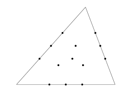
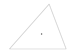
Figure 6.1: The basis of velocity(left) and pressure(right) in any element for Example 1.

Figure 6.2(a) shows that for Example 1, $\eta_{G}(\mathcal{T}_{m})$ has different convergent rates with respect to the degrees of freedom ($d.o.f$) for different $\theta$. Table 6.1 shows the computation cost for different $\theta$ when $\|(\boldsymbol{u}-\hat{\boldsymbol{u}},p-\hat{p})\|_{V}<0.25$. From the comparison in Table 6.1, adaptive FEM is much faster than the uniform refinement. In the MARK step, we set the Döfler parameter as $\theta=0.7$. In the REFINE step, the refinement process is implemented using the MATLAB function REFINEMESH. The key is dividing the marked element into four parts by regular refinement (dividing all edges of the selected triangles in half).

Figure 6.2(b) shows the convergent rates of $\|(\boldsymbol{u}-\hat{\boldsymbol{u}},p-\hat{p})\|_{V}$ and $\eta_{G}(\mathcal{T}_{m})$ for Algorithm 5.1. The $x$-axes denotes the $d.o.f$ in log scale, while $y$-axes denotes the errors in log scale. The squared line denotes the error $\|(\boldsymbol{u}-\hat{\boldsymbol{u}},p-\hat{p})\|_{V}$ of the uniform refinement. The asterisk line and the circled line denote the error $\|(\boldsymbol{u}-\hat{\boldsymbol{u}},p-\hat{p})\|_{V}$ and $\eta_{G}(\mathcal{T}_{m})$ of adaptive FEM, respectively. It is obvious that $\|(\boldsymbol{u}-\hat{\boldsymbol{u}},p-\hat{p})\|_{V}$ and $\eta_{G}(\mathcal{T}_{m})$ have the same convergence order and have a higher convergence order than the uniform refinement.

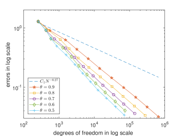
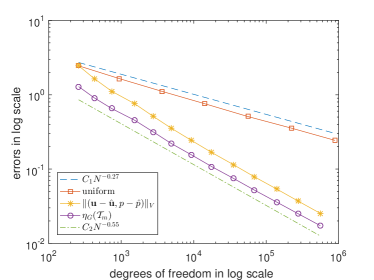
(a)                                                              (b)

Figure 6.2: The convergent rates of adaptive FEM for Example 1.

Table 6.1: Computation cost for different $\theta$ in Example 1.

$\theta$	refinement steps	$d.o.f$	$\|(\boldsymbol{u}-\hat{\boldsymbol{u}},p-\hat{p})\|_{V}$	time(s)
$0.9$	$7$	$31063$	$0.243$	$6.533$
$0.8$	$7$	$14935$	$0.243$	$4.339$
$0.7$	$7$	$9250$	$0.244$	$3.299$
$0.6$	$7$	$6148$	$0.244$	$3.018$
$0.5$	$7$	$4738$	$0.245$	$2.308$
$uniform$	$7$	$887299$	$0.243$	$130.463$

Table 6.2 shows the error $\|(\boldsymbol{u}-\hat{\boldsymbol{u}},p-\hat{p})\|_{V}$, the global error estimator $\eta_{G}(\mathcal{T}_{m})$, and the effective index $\kappa_{eff}$ of the adaptive FEM as the $d.o.f$ increases. The results of effective index $\kappa_{eff}$ defined in (5.3) are shown in the sixth column. The effective index $\kappa_{eff}$ is between $0.5$ and $0.7$ with adaptive refinement, which shows the adaptive FEM is reliable. Figure 6.3 shows the initial mesh with $d.o.f=259$, fourth refinement mesh with $d.o.f=2778$, and seventh refinement mesh with $d.o.f=17707$. It has inserted refinement elements around the singularity at $(x,y)=(0,0)$ as $d.o.f$ increases to reduce the global error.

Table 6.2: The errors, the global error estimator, and the effective index of the adaptive FEM in Example 1.

$d.o.f$	$\|(\boldsymbol{u}-\hat{\boldsymbol{u}},p-\hat{p})\|_{V}$	order	$\eta_{G}(\mathcal{T}_{m})$	order	$\kappa_{eff}$
$259$	$2.452$E0	—	$1.286$E0	—	0.524
$426$	$1.644$E0	$0.803$	$9.068$E-1	$0.702$	0.551
$738$	$1.116$E0	$0.705$	$6.526$E-1	$0.598$	0.584
$1523$	$7.595$E-1	$0.531$	$4.550$E-1	$0.497$	0.599
$2778$	$5.101$E-1	$0.662$	$3.151$E-1	$0.611$	0.617
$4871$	$3.559$E-1	$0.640$	$2.215$E-1	$0.627$	0.622
$9250$	$2.436$E-1	$0.590$	$1.557$E-1	$0.549$	0.639
$17707$	$1.670$E-1	$0.581$	$1.078$E-1	$0.565$	0.645
$35236$	$1.145$E-1	$0.547$	$7.492$E-2	$0.529$	0.653
$68949$	$7.846$E-2	$0.564$	$5.194$E-2	$0.545$	0.661
$138420$	$5.381$E-2	$0.535$	$3.590$E-2	$0.524$	0.667
$277820$	$3.687$E-2	$0.548$	$2.492$E-2	$0.529$	0.675
$557663$	$2.529$E-2	$0.540$	$1.728$E-2	$0.525$	0.683

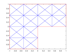
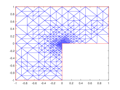
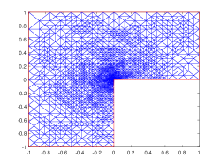
Figure 6.3: The meshes with $d.o.f=259$ (left), $2778$ (middle), and $17707$ (right) for Example 1.

Example 2. In this case, we test the lid-driven cavity problem. The domain is taken as the square $\Omega=(0,1)\times(0,1)$, we set $\boldsymbol{f}=\boldsymbol{0}$, and the boundary conditions $\boldsymbol{u}=0$ on $[\{0\}\times(0,1)]\cup[(0,1)\times\{0\}]\cup[\{1\}\times(0,1)]$ and $\boldsymbol{u}=(1,0)^{T}$ on $(0,1)\times\{1\}$. This problem has a corner singularity. The tangential component of velocity $\boldsymbol{u}\cdot\boldsymbol{\tau}$ has a discontinuity at the two top corners, where $\boldsymbol{\tau}$ denotes the unit tangential vector on the boundary. We use the proposed adaptive FEM algorithm to solve this problem. The finite element space, Döfler parameter, and refinement criterion are the same as Example 1. Figure 6.4 shows that the refinement of mesh focuses on the two top corners. In Figure 6.5, we depict the discrete pressure field obtained using the initial and adapted meshes where we note the improvement in the quality of the computed solution since the singular nature of the pressure is better captured in the adapted mesh.

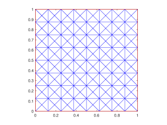
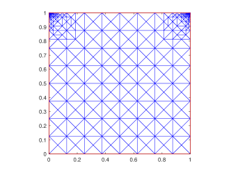
Figure 6.4: The initial mesh and tenth refinement mesh for Example 2.

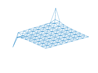
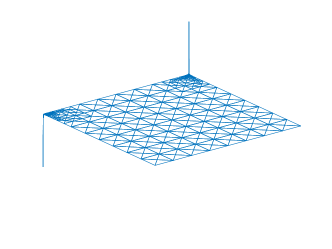
Figure 6.5: The pressures in initial mesh and tenth refinement mesh for Example 2.

7 Conclusion

In this paper, we present an adaptive FEM for solving the Stokes problem with Dirichlet boundary condition. Based on auxiliary subspace techniques, we proposed a hierarchical basis a posteriori error estimator, which is most efficient and robust. We need to solve only two global diagonal linear systems. In theory, The estimator is proved to have global upper and lower bounds without saturation assumption. Numerical experiments are shown to illustrate the efficiency and reliability of our adaptive algorithm.

Declarations

Conflict of interest The authors have no conflicts of interest to declare.
 
Data Availability Data sharing is not applicable to this article as no datasets were generated or analysed during the current study.

Appendix A.

The proof of Lemma 2.2.

Proof

The idea of proof is similar to BOFFI1994 for $d=2$ and BOFFI1997 for $d=3$. Next, we will give proofs for $d=2$ and $d=3$, respectively.

Case $d=2$: The idea is to consider a macroelement partition of the domain $\Omega$ in such a way that each macroelement contains exactly three triangles. By virtue of Remark 3.3 in BOFFI1994 , it suffices to prove the inf-sup condition for only one macroelement. We consider a macroelement $\Omega_{i}=a\cup b\cup c$ as in Figure A.1

Figure A.1: The macroelement partition containing three triangles.

Let us introduce some notations. We denote by $\lambda_{AB}^{a}$ by the barycentric coordinate related to the triangle a, which vanishes on the edge $AB$ (analogous notations for the other cases). we denote by $L_{i,x}^{a}$ the $i$-th Legendre polynomial with respect to the measure $\mu_{a,x}$ defined as

$$\int_{x_{A}}^{0}f(x)d\mu_{a,x}=\int_{a}\lambda_{AB}^{a}\lambda_{AE}^{a}f(x)dxdy\quad\forall f(x):[x_{A},0]\rightarrow\mathbb{R},$$ (A.1)

where $x_{A}$ is the $x$-coordinate of the vertex $A$. A similar definition will hold for $L_{i,y}^{c}$ using $\lambda_{BC}\lambda_{CD}$. On the triangle $b$ we shall use both $L_{i,x}^{b}$ (using $\lambda_{ED}\lambda_{BD}$) and $L_{i,y}^{b}$ (using $\lambda_{BE}\lambda_{ED}$). These Legendre polynomials are defined up to a constant factor so that we can normalize them by imposing that they assume the same value at the origin. This is possible by virtue of Proposition 2.1 in BOFFI1994 .

Our approach to the stability condition will be related to the modified inf-sup condition that can be written as

$$\sup_{\hat{\boldsymbol{v}}\in\overline{WV}_{k+j+1}}\frac{b(\hat{\boldsymbol{v}},\hat{q})}{\|\hat{\boldsymbol{v}}\|}\geq\mu\|\nabla\hat{q}\|,\quad\forall\hat{q}\in\overline{P}_{k+j},$$

which implies the standard one Verfurth1984 .

For every fixed $\hat{q}\in\overline{P}_{k+j}$ we want to construct $\hat{\boldsymbol{v}}\in\overline{WV}_{k+j+1}$ such that

$$-\int_{\Omega}\hat{\boldsymbol{v}}\cdot\nabla\hat{q}dx \geq c_{1}\|\nabla\hat{q}\|^{2},$$ (A.2)

$$\|\hat{\boldsymbol{v}}\|_{0,\Omega} \leq c_{2}\|\nabla\hat{q}\|.$$ (A.3)

Define:

$$\hat{\boldsymbol{v}}(x,y)=(\hat{v}_{1}(x,y),\hat{v}_{2}(x,y)),$$

$$\hat{v}_{1}(x,y)_{|_{a}}=-\lambda_{AB}^{a}\lambda_{AE}^{a}\|\nabla\hat{q}\|L_{k-1,x}^{a}\cdot sign(H_{a}),$$

$$\hat{v}_{2}(x,y)_{|_{a}}=-\lambda_{AB}^{a}\lambda_{AE}^{a}\frac{\partial\hat{q}}{\partial y},$$

$$\hat{v}_{1}(x,y)_{|_{b}}=-\lambda_{ED}^{b}\lambda_{BD}^{b}\|\nabla\hat{q}\|L_{k+d-1,x}^{b}\cdot sign(H_{b})-\lambda_{ED}^{b}\lambda_{EB}^{b}\frac{\partial\hat{q}}{\partial x},$$

$$\hat{v}_{2}(x,y)_{|b}=-\lambda_{EB}^{b}\lambda_{BD}^{b}\frac{\partial\hat{q}}{\partial y}-\lambda_{EB}^{b}\lambda_{ED}^{b}\|\nabla\hat{q}\|L_{k+d-1,y}\cdot sign(K_{b}),$$

$$\hat{v}_{1}(x,y)_{|_{c}}=-\lambda_{BC}^{c}\lambda_{CD}^{c}\frac{\partial\hat{q}}{\partial x},$$

$$\hat{v}_{2}(x,y)_{|_{c}}=-\lambda_{BC}^{c}\lambda_{CD}^{c}\|\nabla\hat{q}\|L_{k+d-1,y}\cdot sign(K_{c}),$$

where $sign(x)$ is sign function defined as

$$sign(x)=\begin{cases}1,&x>0,\\ 0,&x=0,\\ -1,&x<0.\end{cases}$$

and

$$H_{a}=\int_{a}\lambda_{AB}^{a}\lambda_{AE}^{a}L_{k+d-1,x}\cdot\frac{\partial\hat{q}}{\partial x},\quad H_{b}=\int_{b}\lambda_{ED}^{b}\lambda_{BD}^{b}L_{k+d-1,x}\cdot\frac{\partial\hat{q}}{\partial x},$$

$$K_{a}=\int_{b}\lambda_{EB}^{b}\lambda_{ED}^{b}L_{k+d-1,y}\cdot\frac{\partial\hat{q}}{\partial y},\quad K_{b}=\int_{c}\lambda_{BC}^{c}\lambda_{CD}^{c}L_{k+d-1,y}\cdot\frac{\partial\hat{q}}{\partial y}.$$

First of all, we observe that $\hat{\boldsymbol{v}}$ is an element of $\overline{WV}_{k+j+1}$, by the virtue of the fact that the tangential components of $\nabla\hat{q}$ along the interface $EB$ and $BD$ are continuous.

It is easy to verify that $\hat{\boldsymbol{v}}$ satisfies (A.3). In order to check the validity of (A.2), define $|\!|\!|\nabla\hat{q}|\!|\!|=-\int_{\Omega}\hat{\boldsymbol{v}}\cdot\nabla\hat{q}$. Then

$$|\!|\!|\nabla\hat{q}|\!|\!|^{2}= \int_{a}\lambda_{AB}^{a}\lambda_{AE}^{a}(\frac{\partial\hat{q}}{\partial y})^{2}+\|\nabla\hat{q}\|(|H_{a}|+|H_{b}|)$$

$$+\int_{b}\big{(}\lambda_{ED}^{b}\lambda_{EB}^{b}(\frac{\partial\hat{q}}{\partial x})^{2}+\lambda_{ED}^{b}\lambda_{BD}^{b}(\frac{\partial\hat{q}}{\partial y})^{2}\big{)}$$ (A.4)

$$+\|\nabla\hat{q}\|(|K_{a}|+|K_{b}|)+\int_{c}\lambda_{BC}^{c}\lambda_{CD}^{c}(\frac{\partial\hat{q}}{\partial x})^{2}.$$

We verify that the expression $\|\frac{\partial\hat{q}}{\partial x}\|_{H}:=|H_{a}|+|H_{b}|$ is a norm of $\frac{\partial\hat{q}}{\partial x}$ in $a\cup b$ and $\|\frac{\partial\hat{q}}{\partial y}\|_{K}:=|K_{a}|+|K_{b}|$ is a norm of $\frac{\partial\hat{q}}{\partial y}$ in $b\cup c$.

Step 1. We will show $|H_{a}|+|H_{b}|$ vanishes only when $\frac{\partial\hat{q}}{\partial x}$ equals zero. From (A.1)

$$0=\|\frac{\partial\hat{q}}{\partial x}\|_{H}=|\int_{x_{A}}^{0}L_{k+d-1,x}\cdot\frac{\partial\hat{q}}{\partial x}|+|\int_{0}^{1}L_{k+d-1,x}\cdot\frac{\partial\hat{q}}{\partial x}|$$

From the orthogonality of Legendre polynomials $L_{i,x}^{a},L_{i,x}^{b}$ and noting that $\frac{\partial\hat{q}}{\partial x}$ is a homogeneous polynomial of degree $k+d-1$, we have $\frac{\partial\hat{q}}{\partial x}=0$ in $a\cup b$.

Step 2. We will get $\|k\frac{\partial\hat{q}}{\partial x}\|_{H}=|k|\|\frac{\partial\hat{q}}{\partial x}\|_{H}$ from

$$\|k\frac{\partial\hat{q}}{\partial x}\|_{H}=|\int_{x_{A}}^{0}L_{k+d-1,x}\cdot k\frac{\partial\hat{q}}{\partial x}|+|\int_{0}^{1}L_{k+d-1,x}\cdot k\frac{\partial\hat{q}}{\partial x}|.$$

Step 3. We will show that $\|\frac{\partial\hat{q}_{1}}{\partial x}+\frac{\partial\hat{q}_{2}}{\partial x}\|_{H}\leq\|\frac{\partial\hat{q}_{1}}{\partial x}\|_{H}+\|\frac{\partial\hat{q}_{2}}{\partial x}\|_{H}$.

$$\|\frac{\partial\hat{q}_{1}}{\partial x}+\frac{\partial\hat{q}_{2}}{\partial x}\|_{H} =|\int_{x_{A}}^{0}L_{k+d-1,x}\cdot(\frac{\partial\hat{q}_{1}}{\partial x}+\frac{\partial\hat{q}_{2}}{\partial x})|+|\int_{0}^{1}L_{k+d-1,x}\cdot(\frac{\partial\hat{q}_{1}}{\partial x}+\frac{\partial\hat{q}_{2}}{\partial x})|$$

$$\leq|\int_{x_{A}}^{0}L_{k+d-1,x}\cdot\frac{\partial\hat{q}_{1}}{\partial x}|+|\int_{x_{A}}^{0}L_{k+d-1,x}\cdot\frac{\partial\hat{q}_{2}}{\partial x}|+|\int_{0}^{1}L_{k+d-1,x}\cdot\frac{\partial\hat{q}_{2}}{\partial x}|+|\int_{0}^{1}L_{k+d-1,x}\cdot\frac{\partial\hat{q}_{1}}{\partial x}|$$

$$=\|\frac{\partial\hat{q}_{1}}{\partial x}\|_{H}+\|\frac{\partial\hat{q}_{2}}{\partial x}\|_{H}.$$

Similarly, $\|\frac{\partial\hat{q}}{\partial y}\|_{K}=|K_{b}|+|K_{c}|$ is a norm of $\frac{\partial\hat{q}}{\partial y}$ in $b\cup c$. From the equivalence of norms on a finite dimensional space, there exists a constant $C_{a},C_{b},C_{c},C_{H},C_{K}>0$ such that

$$\int_{a}\lambda_{AB}^{a}\lambda_{AE}^{a}(\frac{\partial\hat{q}}{\partial y})^{2}\geq C_{a}\int_{a}(\frac{\partial\hat{q}}{\partial y})^{2},\quad\|\frac{\partial\hat{q}}{\partial x}\|_{H}\geq C_{H}\sqrt{\int_{a}(\frac{\partial\hat{q}}{\partial x})^{2}+\int_{b}(\frac{\partial\hat{q}}{\partial x})^{2}},$$

$$\int_{b}\big{(}\lambda_{ED}^{b}\lambda_{EB}^{b}(\frac{\partial\hat{q}}{\partial x})^{2}+\lambda_{ED}^{b}\lambda_{BD}^{b}(\frac{\partial\hat{q}}{\partial y})^{2}\big{)}\geq C_{b}\int_{b}\big{(}(\frac{\partial\hat{q}}{\partial x})^{2}+(\frac{\partial\hat{q}}{\partial y})^{2}\big{)}$$

$$\int_{c}\lambda_{BC}^{c}\lambda_{CD}^{c}(\frac{\partial\hat{q}}{\partial x})^{2}\geq C_{c}\int_{c}(\frac{\partial\hat{q}}{\partial x})^{2},\quad\|\frac{\partial\hat{q}}{\partial y}\|_{H}\geq C_{K}\sqrt{\int_{b}(\frac{\partial\hat{q}}{\partial y})^{2}+\int_{c}(\frac{\partial\hat{q}}{\partial y})^{2}}.$$

Set $c_{1}=\min\{C_{a},C_{b},C_{c},C_{H},C_{K}\}$ and obtain (A.2).

Case $d=3$: We use the macroelement described by Stenberg in Stenberg1987 in order to check the inf-sup condition. Let $\mathcal{M}$ be a macroelement partition of the domain decomposition of $\mathcal{T}$. For a macroelement $M\in\mathcal{M}$ we introduce the following usual notation:

$$WV_{M}=\{\hat{\boldsymbol{v}}_{|M}~{}|~{}\hat{\boldsymbol{v}}\in W_{k+d+1}\}\cap[H_{0}^{1}(M)]^{3},$$

$$WP_{M}=\{\hat{q}_{|M}~{}|~{}\hat{q}\in WP_{k+d}\}.$$

Consider a generic macroelement $M\in\mathcal{M}$. Let $T_{0}\in\mathcal{T}$ be a tetrahedron of $M$ and denote by $x_{0}$ the internal vertex of $T_{0}$ which also belongs to the other element of $M$. There are three edges $e_{i},i=1,\cdots,3$ of $T_{0}$ meeting at $x_{0}$. Thanks to the fact that $x_{0}$ is internal, none of the edges $e_{i}$ lie on the boundary $\partial\Omega$.

Let $\hat{q}\in WP_{M}$ be given and suppose that

$$\int_{M}\hat{q}\nabla\cdot\hat{\boldsymbol{v}}=0,\quad\forall\hat{\boldsymbol{v}}\in WV_{M}.$$ (A.5)

We shall prove that $\nabla\hat{q}$ vanishes on $T_{0}$, thus obtaining H1 condition described in Theorem 2.1 in BOFFI1997 by virtue of the fact that $T_{0}$ is arbitrary and $q$ is continuous.

First, we concentrate our attention on the edge $e_{1}$ and fix an $(x,y,z)$-coordinate system in such a way that $e_{1}$ lies in the direction of the $x$-axis. We consider the collection $\mathcal{A}=\{T_{0},\cdots,T_{n}\}$ of those elements of $\mathcal{T}$ which share the edge $e_{1}$ in common with $T_{0}$ (including $T_{0}$ itself). It is clear that $T_{i}\in M$ and that exactly two faces of $T_{i}$ touch other elements of $\mathcal{A}$ of every $i$.

Define $\hat{\boldsymbol{v}}$ in the following way:

$$\hat{\boldsymbol{v}}_{|T_{i}}=\big{(}\lambda_{i}\kappa_{i}\frac{\partial\hat{q}}{\partial x},0,0\big{)},$$

$$\hat{\boldsymbol{v}}_{|T}=(0,0,0),\quad\mbox{~{}if~{}}T\in\mathcal{T},~{}T\neq T_{i},~{}\forall i,$$

where $\lambda_{i}$ and $\kappa_{i}$ are the equations of the two faces of $T_{i}$ which are not in common with any other element of $\mathcal{A}$, normalized in order to assume the same value at the opposite vertex. It is worthwhile to observe that these two vertices are $x_{0}$ and the other extreme of the edge $e_{1}$.

It is easily verified that $\hat{\boldsymbol{v}}$ is a polynomial of degree $k+1$ and that it is continuous in $M$. The continuity of $\hat{q}$ in $M$ ensures that the gradient of $\hat{q}$ is continuous between two elements in all the directions which are contained in the plane of the interface; the $x$-axis is the direction of $e_{1}$ which is the edge of all common faces among the elements of $\mathcal{A}$. Moreover, $\hat{\boldsymbol{v}}$ vanishes at the boundary of $M$; hence, the following inclusion holds:

$$\hat{\boldsymbol{v}}\in WV_{M}.$$

Suppose now that (A.5) hold.

$$0=\int_{M}\hat{q}\nabla\hat{\boldsymbol{v}}=-\int_{M}\nabla\hat{q}\cdot\hat{\boldsymbol{v}}=-\sum_{i=1}^{n}\int_{T_{i}}\lambda_{i}\kappa_{i}(\frac{\partial\hat{q}}{\partial x})^{2}.$$

It follows that the component of $\nabla\hat{q}$ in the direction of the $x$-axis vanishes in $T_{i}$ for every $i$.

The same argument applies to the edge $e_{2}$ and $e_{3}$, giving the result that $\nabla\hat{q}$ vanishes on $T_{0}$ in the direction of $e_{i}$, for $i=1,\cdots,3$. These three directions being independent, the final result

$$\nabla\hat{q}=(0,0,0),\quad\mbox{~{}in~{}}T_{0}$$

is obtained and the lemma is proved. Then the H1 condition of Theorem 2.1 in BOFFI1997 is proved and the H2-H3 conditions follow immediately from the regularity assumption of $\mathcal{T}$.

References

- (1) Antonietti, P.F., da Veiga, L.B., Lovadina, C., Verani, M.: Hierarchical A Posteriori Error Estimators for the Mimetic Discretization of Elliptic Problems. SIAM Journal on Numerical Analysis 51(1), 654–675 (2013)
- (2) Araya, R., Barrenechea, G.R., Poza, A.: An adaptive stabilized finite element method for the generalized Stokes problem. Journal of Computational and Applied Mathematics 214(2), 457–479 (2008)
- (3) Araya, R., Poza, A.H., Stephan, E.P.: A hierarchical a posteriori error estimate for an advection-diffusion-reaction problem. Mathematical Models and Methods in Applied Sciences 15(7), 1119–1139 (2005)
- (4) Araya, R., Poza, A.H., Valentin, F.: On a hierarchical error estimator combined with a stabilized method for the Navier-Stokes equations. Numerical Methods for Partial Differential Equations 28(3), 782–806 (2012)
- (5) Araya, R., Rebolledo, R.: An a posteriori error estimator for a LPS method for Navie-Stokes equations. Applied Numerical Mathematics 127, 179–195 (2018)
- (6) Arnold, D.N.: Spaces of Finite Element Differential Forms. In: Brezzi, F., Colli-Franzone, P., Gianazza, U.P., Gilardi, G. (eds.) Analysis and Numerics of Partial Differential Equations, Springer INdAM Series, vol. 4. Springer, Milan (2013)
- (7) Babuška, I., Aziz, A.: Survey lectures on the mathematical foundations of the finite element method, in The Mathematical Foundations of the Finite Element Method with Applications to Partial Differential Equations. Academic Press, New York, NY (1972)
- (8) Boffi, D.: Stability of higher order triangular Hood-Taylor methods for the stationary Stokes equations. Mathematical Models and Methods in Applied Sciences 04(2), 223–235 (1994)
- (9) Boffi, D.: Three-Dimensional Finite Element Methods for the Stokes Problem. SIAM Journal on Numerical Analysis 34(2), 664–670 (1997)
- (10) Boffi, D., Brezzi, F., Demkowicz, L.F., Durán, R.G., Falk, R.S., Fortin, M.: Mixed Finite Elements, Compatibility Conditions, and Applications, Lecture Notes in Mathematics, vol. 1939. Springer Berlin Heidelberg, Berlin, Heidelberg (2008)
- (11) Bornemann, F.A., Erdmann, B., Kornhuber, R.: A posteriori error estimates for elliptic problems in two and three space dimensions. SIAM Journal on Numerical Analysis 33(3), 1188–1204 (1996)
- (12) Dörfler, W.: A Convergent Adaptive Algorithm for Poisson’s Equation. SIAM Journal on Numerical Analysis 33(3), 1106–1124 (1996)
- (13) Dörfler, W., Nochetto, R.H.: Small data oscillation implies the saturation assumption. Numerische Mathematik 91(1), 1–12 (2002)
- (14) Eijkhout, V., Vassilevski, P.: The Role of the Strengthened Cauchy-Buniakowskii-Schwarz Inequality in Multilevel Methods. SIAM Review 33(3), 405–419 (1991)
- (15) Giani, S., Grubišić, L., Hakula, H., Ovall, J.S.: A Posteriori Error Estimates for Elliptic Eigenvalue Problems Using Auxiliary Subspace Techniques. Journal of Scientific Computing 88(3) (2021)
- (16) Hain, S., Ohlberger, M., Radic, M., Urban, K.: A hierarchical a posteriori error estimator for the Reduced Basis Method. Advances in Computational Mathematics 45, 2191–2214 (2019)
- (17) Hakula, H., Neilan, M., Ovall, J.S.: A Posteriori Estimates Using Auxiliary Subspace Techniques. Journal of Scientific Computing 72(1), 97–127 (2017)
- (18) Huang, W., Russell, R.D.: Adaptive Moving Mesh Methods, Applied Mathematical Sciences, vol. 174. Springer, New York (2011)
- (19) Nochetto, R.H., Siebert, K.G., Veeser, A.: Theory of adaptive finite element methods: An introduction. Multiscale, Nonlinear and Adaptive Approximation: Dedicated to Wolfgang Dahmen on the Occasion of his 60th Birthday pp. 409–542 (2009)
- (20) Pfeiler, C.m., Praetorius, D.: Dörfler marking with minimal cardinality is a linear complexity problem. Mathematics of Computation 89(326), 2735–2752 (2020)
- (21) Scott, L.R., Zhang, S.: Finite Element Interpolation of Nonsmooth Functions Satisfying Boundary Conditions. Mathematics of Computation 54(190), 483 (1990)
- (22) Stenberg, R.: On some three-dimensional finite elements for incompressible media. Computer Methods in Applied Mechanics and Engineering 63(3), 261–269 (1987)
- (23) Verfürth, R.: Error estimates for a mixed finite element approximation of the Stokes equations. RAIRO. Analyse numérique 18(2), 175–182 (1984)
- (24) Verfürth, R.: A review of a posteriori error estimation and adaptive mesh-refinement techniques. Teubner, Stuttgart (1996)
- (25) Verfürth, R.: A Posteriori Error Estimation Techniques for Finite Element Methods. Oxford University Press, Oxford (2013)
- (26) Zienkiewicz, O., Graig, A.: Adaptive refinement, errorestimates, multigrid solution and hierarchical finite element method concepts. Accuracy Estimates and Adaptive Refinements in Finite Element Computations, John Wiley and Sons pp. 25–59 (1986)
- (27) Zienkiewicz, O., Kelly, D., Gago, J., Babuška, I.: Hierarchical finite element approaches, error estimates and adaptive refinemen. The Mathematics of Finite Elements and Applications IV, Academic Press pp. 313–346 (1982)