Optimal Covariate Weighting Increases Discoveries in High-throughput Biology

Abstract

The large-scale multiple testing inherent to high throughput biological data necessitates very high statistical stringency and thus true effects in data are difficult to detect unless they have high effect sizes. One promising approach for reducing the multiple testing burden is to use independent information to prioritize the features most likely to be true effects. However, using the independent data effectively is challenging and often does not lead to substantial gains in power. Current state-of-the-art methods sort features into groups by the independent information and calculate weights for each group. However, when true effects are weak and rare (the typical situation for high throughput biological studies), all groups will contain many null tests and thus their weights are diluted, and performance suffers. We introduce Covariate Rank Weighting (CRW), a method for calculating approximate optimal weights conditioned on the ranking of tests by an external covariate. This approach uses the probabilistic relationship between covariate ranking and test effect size to calculate individual weights for each test that are more informative than group weights and are not diluted by null effects. We show how this relationship can be calculated theoretically for normally distributed covariates. It can be estimated empirically in other cases. We show via simulations and applications to data that this method outperforms existing methods by as much as 10-fold in the rare/low effect size scenario common to biological data and has at least comparable performance in all scenarios.

Keywords: multiple testing; high-throughput; weighted p-value; covariate.

1 Introduction

The rise of high throughput techniques has dramatically increased the resolution of biological data, often approaching the maximum possible for the data type (e.g., all genes in an organism or all nucleotide positions in a genome). The promise of this data is that it allows researchers to test very large numbers of biological features for effects of interest cheaply and easily. However, although this opens many new opportunities for discoveries, it creates a “needle in haystack” problem. Most features are not relevant to any particular question at hand, and thus high throughput data requires searching large numbers of features for small numbers of effects.

Increasing the number of data features involves a tradeoff: on the one hand, it increases the opportunities to find interesting effects; on the other hand, each additional feature decreases the probability of successfully detecting effects already present in the data. For this reason, the loss of per-feature statistical power often outweighs the benefits of an increased number of data features. Across many data types, most effects of interest are weak and cannot be detected with reasonable sample sizes after a large multiple testing correction.

One solution to this problem is using other sources of data to prioritize the most promising hypothesis tests. With the prevalence of comprehensive databases in many realms of biology, such data sources abound. For example, genetic variants in a genome-wide association study could be prioritized using information such as 1) markers at nucleotide positions that are more evolutionarily constrained may be better candidates than positions that are less evolutionarily constrained; 2) genetic markers that lie near genes that have previously been found to be differentially expressed for a trait of interest may be good candidates for being causative for the trait; 3) markers that had suggestive (but not conclusive) evidence for association to a trait in past studies might be good candidates in future studies.

In a concrete example, Kim and Schliekelman (2015) were looking for genetic markers linked to body weight in mice. They used the Mouse Gene Expression Database to identify $37$ genes whose expression had been associated with body weight in previous studies. A marker that is causative for expression for such a gene is a good candidate for being causative for body weight. Thus, they used a gene expression data set to find a score for the strength of effect of each marker on the $37$ genes. A high score indicates strong evidence that the marker is causative for expression for some of the $37$ bodyweight genes and thus is a promising target. This score was used as a covariate to prioritize markers and increase discoveries. Such covariates exist across many types of data and are easily identified by researchers in those areas.

However, it remains an open question how to use external data best to prioritize data features. Weighted p-values have been one of the most widely used approaches. In p-value weighting, weights are calculated for each p-value, with larger weights for more promising tests.

Consider a situation in which there are $m$ hypothesis tests, and we want test the null hypothesis $H_{0i}:\varepsilon_{i}=0$ against the alternative hypothesis $H_{ai}:\varepsilon_{i}>0;i=1,\ldots,m,$ where the effect size is $\varepsilon_{i}=\sqrt{n_{i}}\mu_{i}/\sigma_{i}$ for the $i$th alternative mean $\mu_{i}$ with corresponding sample size $n$ and standard deviation $\sigma$. For illustrative purpose, we consider only one-sided test; however, one can easily generalize to two-sided test. Define a set of p-values $P=\{p_{1},\ldots,p_{m}\}$. If $R$ and $H_{0}$ refer to the set of rejected null and true null hypothesis, respectively, then $R$ controls the Family Wise Error Rate (FWER) if $P(R\cap H_{0})\leq\alpha$.

Next, define a a set of non-negative weights $w=\{w_{1},\ldots,w_{m}\}$. Then, the simple Bonferroni weighted procedure (Rosenthal and Rubin, 1983; Genovese et al., 2006) rejects a null hypothesis $i$ if

$$i\ \epsilon\ R=\Big{\{}i:\frac{P_{i}}{w_{i}}\leq\frac{\alpha}{m}\Big{\}},$$

This weighting scheme will control FWER if the average weight is $1$ (Roeder and Wasserman, 2009). Similarly, Genovese et al. (2006) showed that a weighted FDR procedure can be easily conducted by using weighted p-values in the procedure of Benjamini and Hochberg (1995).

The larger the weight, the smaller the weighted p-value and thus the higher chance of rejecting the null hypothesis. If the weights are chosen well, then the probability of discovering true effects can be increased. Generally, the goal is to have higher weights for more promising tests and lower weights for less promising tests. Several authors (Roeder et al., 2006; Rubin et al., 2006; Roeder and Wasserman, 2009) have taken the approach of finding the weights that maximize the average power across tests, given the true effect sizes. Then, the optimal weight for a test with effect size $\varepsilon_{i}$ is

$$\hat{w}_{i}=\Big{(}\frac{m}{\alpha}\Big{)}\bar{\Phi}\Big{(}\frac{\varepsilon_{i}}{2}+\frac{c}{\varepsilon_{i}}\Big{)}I(\varepsilon_{i}>0),$$ (1)

where c is a constant so that $\sum_{i=1}^{m}\hat{w}_{i}=m$ and $\Phi=1-\bar{\Phi}$ is the standard normal CDF.

Unfortunately, expression (1) is not directly applicable because it requires knowledge of the effect sizes. These are not generally known - if they were known, there would be no need to conduct the experiment. Rubin et al. (2006) proposed using a data splitting approach to estimate the effect sizes and weights. One can randomly split the data into two parts and use the first part as a training set to estimate $\varepsilon_{i}$ and the corresponding optimal weights. These are then applied to the testing set. Unfortunately, they showed that the power gain from this weighting procedure cannot compensate for the loss of power resulting from the split data.

A solution is to incorporate the independent information discussed above in calculating the weights. Now, suppose that each hypothesis test $i$ has an associated covariate value $Y_{i}$, where $Y_{i}$ is higher for tests that are more likely to be true effects. Various authors have proposed weighting based on such external information (Satagopan et al., 2002; Westfall et al., 2004; Ionita-Laza et al., 2007; Roeder and Wasserman, 2009; Dobriban et al., 2015; Kim and Schliekelman, 2015). Roeder and Wasserman (2009) (RDW) proposed a method of estimating weights by breaking the hypothesis tests into groups based on the covariate, estimating effect sizes for each group from the data, and then using (1) to calculate weights for each group. To maintain FWER control, the group sizes must be large enough so that individual null features with chance large test statistics will not inflate estimates of effects, thus boosting themselves erroneously.

Recently, Ignatiadis et al. (2016) introduced an innovative method that they term independent hypothesis weighting (IHW). Hypothesis tests are split into groups by an independent covariate that is believed to provide information about statistical properties of the hypothesis tests. Weights are calculated for each group based on a computational approach that maximizes the number of rejections while maintaining a pre-specified FDR. A key component of IHW is that the hypothesis tests are split into $k$ folds. For each fold, the IHW optimization procedure is applied to the other $k-1$ folds, and the resulting weights are applied to the remaining fold. Thus, the weights for each fold do not depend on p-values in the fold itself. Without this procedure, the FWER control would be lost because a chance small p-value in a group would tend to inflate the weight and thus erroneously elevate itself to significance.

Although this method is powerful, we will demonstrate that IHW, RDW, and other group-based methods have diminished performance in the case that true effects are uncommon (e.g., under $20\%$ of all tests) or the power to detect them is low (i.e., most high throughput datasets). Then, true effects of interest are difficult to distinguish from the background of null tests. When groups are formed according to the covariate, even the best-ranked groups will have many null tests. Because weights are based on group properties, the weights will be diluted by the effect of the null tests. Unfortunately, very low power is almost universal in high throughput biological data. Strong signals are rare and usually already discovered, and the high multiple testing correction intrinsic to high throughput data makes power low for detection of anything but strong signals.

An alternative approach is to weight groups based using a mathematical function based on some criterion that is assumed to provide good weighting. Westfall et al. (2004) proposed the use of certain data-driven quadratic forms. Ionita-Laza et al. (2007) proposed an exponential weighting scheme for tests sorted by an external covariate. Each subsequent group is twice the size of the previous one, and each weight is $1/4$ of the previous one. Kim and Schliekelman (2015) proposed weights based on a vector $\bar{n}$ that defines group boundaries among covariate-sorted p-values and uses weights $w_{j}=m/\lambda n_{k(j)}$, where $n_{k(j)}$ is the smallest value from the vector $\bar{n}$ that is greater than $j$, and $\lambda$ is a coefficient that makes the weights average to one. These approaches are based on predetermined mathematical functions and are not data-driven. The advantage of this is that the weights are not based on groups and do not have the problem of diluted weights that the RDW and IHW methods suffer. On the other hand, the distribution of effect sizes in a data set may not match well with the distribution of the weights.

In this paper, we present a method for calculating p-value weights, Covariate Rank Weighting (CRW), which is not group based but still takes into account properties of the data. CRW is based on covariate information and works well in the scenario in which true effects are rare and low. The starting point for CRW is the optimal weights of Roeder et al. (2006) and Roeder and Wasserman (2009). These oracle weights require knowledge of the true effect sizes, which is not a reasonable requirement. In our method, hypothesis tests are ranked by a covariate. We derive weights that are approximately optimal conditioned on the covariate ranking. Our approach requires knowledge of the probabilistic relationship between true effect size and the ranking of tests by an independent covariate. We derive this relationship for the case of normally distributed covariates. It can be estimated empirically in other cases.

The information in the weights comes from the relationship between the test effect size and the ranking by the covariate. Thus, they are not diluted in high throughput data as group-based weights typically are. We will show that CRW weights have as much as a $10$-fold advantage in power in the low power situation common to high throughput data and are thus the most powerful available method for integrating covariate information into large-scale hypothesis testing.

2 Methods–Covariate rank weighting

2.1 Power formulation

We will now describe our approach for p-value weighting. Suppose there are total $m$ hypothesis tests with $m_{1}$ true effects and $m_{0}=m-m_{1}$ null effects. The goal is to test the null hypothesis $H_{0i}:\varepsilon_{i}=0$ against the alternative hypothesis $H_{1i}:\varepsilon_{i}>0;i=1,\ldots,m$. There is a test statistic $Z_{i}$ associated with each hypothesis test; we assume that this test statistic follows a normal distribution. In addition, each hypothesis test $i$ has an associated covariate $Y_{i}$. This covariate is calculated from some independent data that is believed to contain information about the effect sizes of the hypothesis tests in the sense that hypothesis tests with larger covariate values are more likely to be true alternative tests. We rank the hypothesis tests by the covariate so that each hypothesis test has a covariate rank $r_{i}$. We assume that we know the distribution $f(\varepsilon\mid r_{i})$, the probabilistic relationship between the covariate ranking and the effect size. We can calculate this directly under certain distributional assumptions, or estimate it from data. Our goal is to derive p-value weights based on this quantity. Define $\beta(r_{i};w_{i})$ as the power for the test $i$ with rank $r_{i}$ and weight $w_{i}$:

$$\beta(r_{i};w_{i})=P\big{(}Z_{i}>Z_{\frac{\alpha w_{i}}{m}}\mid r_{i}\big{)}.$$ (2)

We assume that a significance will be determined using a weighted Bonferroni threshold $\alpha w_{i}/m$. Next, we incorporate the random effect size $\varepsilon$ into (2) and apply Bayes rule:

$$\beta(r_{i};w_{i})=\frac{\int{P\big{(}Z_{i}>Z_{\frac{\alpha w_{i}}{m}}\mid r_{i},\varepsilon\big{)}P\big{(}r_{i}\mid\varepsilon\big{)}f\big{(}\varepsilon\big{)}I(\varepsilon>0)d\varepsilon}}{P\big{(}r_{i}\big{)}},$$

where $P(r_{i})$ is the prior probability of the covariate rank, $P(r_{i}\mid\varepsilon)$ is the rank probability conditioned on the effect size $\varepsilon$, $f(\varepsilon)$ is the probability density function of the effect size, and $I(\varepsilon>0)$ is equal to one when the effect size $\varepsilon>0$ and zero otherwise. If the test statistic $Z_{i}$ is normally distributed, then $P\big{(}Z_{i}>Z_{\frac{\alpha w_{i}}{m}}|r_{i},\varepsilon\big{)}=\bar{\Phi}\big{(}Z_{\frac{\alpha w_{i}}{m}}-\varepsilon\big{)}$. $\bar{\Phi}\big{(}\cdot\big{)}$ is equal to one minus the normal CDF. The prior probability of the covariate rank is given by $P(r_{i})=1/m$, because, lacking additional information, all tests are equally likely to receive any covariate rank. This yields the average power

$$\frac{1}{m}\sum_{i=1}^{m}\beta(r_{i};w_{i})=\frac{1}{m}\sum_{i=1}^{m}\int{\bar{\Phi}\big{(}Z_{\frac{\alpha w_{i}}{m}}-\varepsilon\big{)}mP(r_{i}\mid\varepsilon)f(\varepsilon)I(\varepsilon>0)d\varepsilon}.$$ (3)

We will derive expressions for $P(r_{i}\mid\varepsilon)$ later in the paper.

2.2 Weight

In the following theorem we show the proposed approximate optimal weight.

Theorem 1.

Given $P\big{(}r_{i}\mid E(\varepsilon)\big{)}$, the optimal weights that maximize the average power (3) are

$$w_{i}(r_{i};\delta)\approx\Big{(}\frac{m}{\alpha}\Big{)}\bar{\Phi}\Bigg{(}\frac{E(\varepsilon)}{2}+\frac{1}{E(\varepsilon)}log\bigg{(}\frac{\delta}{\alpha P\big{(}r_{i}\mid E(\varepsilon\mid\varepsilon>0)\big{)}}\bigg{)}\Bigg{)},$$ (4)

where $\delta\geq 0$ is the normalizing constant such that $\sum_{i=1}^{m}w_{i}(r_{i};\delta)=m.$

$E(\varepsilon\mid\varepsilon>0)$ refers to the expected value of the effect sizes for the true effects. In order to preserve control of type I error, the average weight must be equal to $1$, i.e. $\sum_{i=1}^{m}w_{i}=m$. The goal is to find the vector of weights $\bar{w}$ that maximizes the average power subject to this constraint. Consider the weight $w_{k}$ for a specific test $k$. We need to maximize the expression below with respect to $w_{k}$:

$$L(w_{i};r_{i})=\frac{1}{m}\sum_{i=1}^{m}\int{\bar{\Phi}\big{(}Z_{\frac{\alpha w_{i}}{m}}-\varepsilon\big{)}mP(r_{i}\mid\varepsilon)f(\varepsilon)I(\varepsilon>0)d\varepsilon}-\delta\Big{(}\frac{1}{m}\sum_{i=1}^{m}w_{i}-1\Big{)},$$

where $\delta$ refers to the Lagrange multiplier. We maximize by differentiating with respect to $w_{k}$, setting equal to zero, and solving. After performing simple algebra, this produces

$$\int\left(e^{Z_{\frac{\alpha w_{k}}{m}\varepsilon}-\frac{\varepsilon^{2}}{2}}\right)P(r_{k}\mid\varepsilon)f(\varepsilon)d\varepsilon=\frac{\delta}{\alpha}.$$ (5)

The above integration is not easily tractable, except for special cases of $P(r_{i}\mid\varepsilon)$ and $f(\varepsilon)$. Numerical solutions of the weights are tractable. However, we obtain an approximate general weight expression that will be applicable in a wide variety of situations. Let

$$g(\varepsilon)=\left(e^{Z_{\frac{\alpha w_{k}}{m}\varepsilon}-\frac{\varepsilon^{2}}{2}}\right)P(r_{k}\mid\varepsilon).$$

Equation (5) can then be interpreted as $E(g(\varepsilon))$. Since $\varepsilon$ is a random variable and $g(\varepsilon)$ is a differentiable function, then $E(g(\varepsilon))=g(E(\varepsilon))$ in the first order Taylor series expansion of $E(g(\varepsilon))$. Consequently, after simple algebraic manipulation, the approximate version of the weight (4) is obtained. With this approximation, the weights maximize the average (over tests) power evaluated at the expected non-zero effect size. Exact weights would maximize the average expectation of power over effect size.

This is similar to the Roeder and Wasserman (2009) weight (1) but incorporates the relationship $P(r_{i}\mid\varepsilon)$. The main advantage of this weight is that it does not require knowledge of the effect sizes. Instead, it only requires the expected value of the effect sizes and the relationship between the effect size and the covariate rank.

Dobriban et al. (2015) generalized the Roeder and Wasserman (2009) weights to the scenario that effect sizes follow a Gaussian distribution with a known mean and variance. They optimized average power in a manner similar to our approach. However, their approach only considers the distribution $f(\varepsilon)$. Our work builds on theirs by explicitly including the covariate rank $r_{i}$. A key advantage of our method is that using the rank distribution explicitly accounts for the other tests in determining how to weight a given test. That is, it uses more information in specifying the weight. These methods will be compared more fully in a future manuscript.

We compared the approximate weights and the exact weights obtained by numerical integration (Figure 18 in SI). Both the approximate and the exact approaches provided similar results. To compute the approximate weights, we used expression (4); and to compute the exact weights, we applied the numerical integration to (5). We applied these procedures to the two datasets shown in Figure 8.

To obtain the optimal value of $\delta$, we applied Newton-Raphson algorithm (NR) when $\varepsilon>1$ and Grid search algorithm when $\varepsilon\ \epsilon\ [0,1)$. Although Newton-Raphson is computationally faster, it is sensitive to a correct guess of the initial value and is also sensitive to non-convexity. When the effect size is low, then the weights are flatter, and the NR method often does not converge. Therefore, we used grid search algorithm to obtain $\delta$ for low $\varepsilon$. The full algorithm for finding $\delta$ is given in the SI (Section 19).

2.3 Rank probability given continuous effect $P(r_{i}\mid\tau_{i})$

The primary source of information in the weights is the probability $P(r_{i}\mid\varepsilon_{i})$, where $r_{i}$ is the rank by the covariate and $\varepsilon_{i}$ is the effect size for the hypothesis test $i$. This quantity determines how the weights vary with covariate rank. The covariate is assumed to have an effect size $\tau_{i}$ that is distinct from the test effect size $\varepsilon_{i}$. Thus, the covariate rank $r_{i}$ depends on the covariate effect size $\tau_{i}$ and not on the test effect size $\varepsilon_{i}$ directly. However, the fundamental assumption of our approach is that there is a positive relationship between the two effect sizes and hence higher values of the covariate indicate more promising tests.

In the following, we will derive the distribution for covariate rank given covariate effect size, $P(r_{i}\mid\tau_{i})$. We will then discuss the relationship between test effect size $\varepsilon_{i}$ and covariate effect size $\tau_{i}$.

Theorem 2.

Suppose there are $m$ hypothesis tests with associated covariate values and $r_{i},r_{0i}$ and $r_{1i}$; $i=1,\ldots,m$ are the ranks of a random covariate value $t$ given the covariate effect size $\tau_{i}$ among covariate values for all tests, among the true nulls, and among the true alternatives, respectively. Then the rank probability $P(r_{i}\mid\tau_{i})$ is the expectation of the pmf of the sum of two Binomial random variables $r_{0i}$ and $r_{1i}$, and the expectation is over $t$. If $t$ is from null, then $r_{1i}\sim binomial(m_{1},F_{1})$ and $r_{0i}\sim binomial(m_{0}-1,F_{0})$, where $F_{0}$ and $F_{1}$ are the CDFs of the covariates under the null and alternative hypotheses, respectively. If $t$ is from alternative hypothesis, then $r_{1i}\sim binomial(m_{1}-1,F_{1})$ and $r_{0i}\sim binomial(m_{0},F_{0})$. The rank probability is given by

$$P(r_{i}=k\mid\tau_{i})=E_{T}\Big{[}\sum_{k_{0}=1}^{k}\left\{P(r_{1i}=k-k_{0}+1\mid\tau_{i},t)P(r_{0i}=k_{0}\mid\tau_{i},t)\right\}\Big{]}$$ (6)

See Appendix 1 for the proof and further discussion. Equation (6) is not easily tractable, and finding a closed form solution is difficult. However, (6) can be solved numerically and can also be easily simulated. We solved (6) using the importance sampling method of the Monte Carlo (MC) simulation. Importance sampling is an MC simulation approach in which the integral is expressed as an expectation of a function of a random variable. Then, the density of the random variable is chosen appropriately to reduce the variance of the estimated integral.

Furthermore, since the term inside the expectation is the sum of two independent binomial random variables, we propose a normal approximation of the term. This approximation introduces a procedure that is faster and easier than many other algorithms:

Proposition 1.

Rank probability $P(r_{i}=k\mid\tau_{i})$ is the expected value of the normal PDF, i.e.,

$$P(r_{i}=k\mid\tau_{i})=\begin{cases}E_{T}N(k-1\mid\mu_{0},\sigma_{0}^{2}),&\text{if }\tau_{i}=0\\ E_{T}N(k-1\mid\mu_{1},\sigma_{1}^{2}),&\text{if }\tau_{i}>0\end{cases},$$

where

$$\begin{cases}\mu_{0}=(m_{0}-1)(1-F_{0})+m_{1}(1-F_{1})+1\\ \mu_{1}=m_{0}(1-F_{0})+(m_{1}-1)(1-F_{1})+1\\ \sigma_{0}=(m_{0}-1)(1-F_{0})F_{0}+m_{1}(1-F_{1})F_{1}\\ \sigma_{1}=m_{0}(1-F_{0})F_{0}+(m_{1}-1)(1-F_{1})F_{1}\end{cases}.$$

$N(k-1\mid\mu_{i},\sigma_{i}^{2})$ represents the normal pdf evaluated at the value $k-1$.

2.4 Relationship between test effect and covariate effect

For each test $i$, take $\varepsilon_{i}$ as the effect size for the test statistic and $\tau_{i}$ as the effect size for the covariate. The information in the weights comes from the relationship between the covariate rank $r_{i}$ and the test effect size $\varepsilon_{i}$, while the covariate rank depends on the covariate effect size $\tau_{i}$. The fundamental assumption of our approach is that there is a positive relationship between the two effect sizes.

In the implementation in this paper, we assume that there is a noisy linear relationship between the test effect size and the covariate effect size. That is,

$$\tau_{i}=\alpha+\beta\varepsilon_{i}+N\big{(}0,\sigma^{2}\big{)}$$ (7)

for some $\alpha$, $\beta$, and $\sigma$. We conduct a linear regression of estimated covariate effect sizes on estimated test effect sizes and then use this to find the corresponding value of the covariate effect (see work flow in SI). This value is then used to calculate the rank probability (6) used in the weight formula (4). The linear model assumption is not fundamental to our approach. It would be straightforward to fit the covariate effect - test effect relationship using a non-linear regression method.

Note that the weight formula (4) only depends on $P\big{(}r_{i}\mid E(\varepsilon\mid\varepsilon>0)\big{)}$. Thus, we only need to identify the covariate effect size corresponding to the mean test effect size among true alternative effects. This is the point at which the regression line is most accurate and also not highly sensitive to deviations from a linear relationship.

In the simulation section, we explore the effect of the noise in the relationship between $\varepsilon_{i}$ and $\tau_{i}$. In the Supplementary Material, we show simulation results for the case that the relationship between test effect and covariate effect is non-linear when we assume that it is linear. A moderate degree of non-linearity does not have a large impact on the performance of our method.

2.5 Weight and rank probability given binary effect $P(r_{i}\mid\varepsilon)$

We also propose weights for binary effects, i.e., estimating weights for $H_{0i}:\varepsilon_{i}=0$ vs. $H_{1i}:\varepsilon_{i}=\varepsilon$ (a fixed value). Therefore, the prior probability of having a true effect is $p=m_{1}/m$. Following similar arguments to the continuous effect size case, we find the following weights:

Corollary 1.

Given $P\big{(}r_{i}\mid\varepsilon)$, the optimal weights that maximize the average power (3) are

$$w_{i}(r_{i};\delta)=\Big{(}\frac{m}{\alpha}\Big{)}\bar{\Phi}\Bigg{(}\frac{\varepsilon}{2}+\frac{1}{\varepsilon}log\bigg{(}\frac{\delta m}{\alpha m_{1}P(r_{i}\mid\varepsilon)}\bigg{)}\Bigg{)}I(\varepsilon_{i}=\varepsilon).$$ (8)

where $\delta\geq 0$ is the normalizing constant such that $\sum_{i=1}^{m}w_{i}(r_{i};\delta)=m.$

The main advantage of the binary case is that it is fairly easy to calculate, and an exact version of the weight is available. One can compute $P(r_{i}\mid\varepsilon)$ in a manner similar to the continuous case.

2.6 Work flow

The full work flow for the CRW method is given in the SI.

2.7 Simulation of dilution effect in group-based methods

We used simulations to explore the performance of group based methods like IHW when true effects are weak and rare. We assumed that there were a total of $m=40,0000$ hypothesis tests. The number of true null tests was $m_{0}=m\pi_{0}$ where $\pi_{0}$, the proportion of null hypothesis, varied between simulations. The number of true alternative tests was $m_{1}=m-m_{0}$. The effect sizes for the true alternative tests were generated from $N(\mu_{\epsilon},1)$, where $\mu_{\epsilon}$ varied for different scenarios. For each hypothesis test, the test statistic and the covariate value were generated from independent normal distribution with mean equal to the effect size and a standard deviation of $1$. Thus, the test statistic and the covariate were correlated across tests due to the shared mean. The tests were then sorted by the covariate and divided evenly into $10$ groups. The proportion of true alternative hypothesis tests and the mean effect size were calculated for the top group and plotted. Next, we conducted a simulation using the IHW method with $10$ groups. Data were simulated in the same manner as above. We used the ihw function from the R package IHW to calculate weights for each group. The IHW weights were plotted as a function of $\pi_{0}$ and $\mu_{\epsilon}$. $100$ simulation replicates were conducted for each combination of $\pi_{0}$ and $\mu_{\epsilon}$ and the mean weight for each group was calculated across replicates.

3 Results

3.1 Power in high throughout studies

First, we demonstrate that low statistical power is pervasive in high throughput biological data. Figure 1 shows the distribution of estimated power across tests for two different datasets: 1) the RNA-seq data of Bottomly et al. (2011) and 2) the proteomics dataset of Dephoure and Gygi (2012). In each dataset, we estimated $m_{1}$, the number of true effect hypothesis tests, using the method of Storey and Tibshirani (2003). We then estimated the effect size for the $m_{1}$ most significant tests from their p-values and calculated the corresponding power assuming that the test statistic follows a normal distribution and using a Bonferroni correction (see SI for the details). Simulations included in the SI (Figure 3.1-3.2) demonstrate that this method is informative about the true distribution of power but will tend to overestimate power. Fig. 1 shows the estimated distribution of the power for the two datasets. Even with the likely overestimate of power, the estimated values are very low for nearly all tests in both datasets.

For the RNA-seq data, the median of estimated power values is $0.08\%$ and the $90\%$ quantile is $10\%$. For the proteomics data, the median is $1\%$ power and the $90\%$ quantile is $17\%$ power. It should be emphasized that these values are only for the tests estimated to be true positive features. This very low power is a result of the multiple testing correction. There are many effects in both datasets that would be strongly significant if they were tested individually but are undetectable when tested with many other features. If we used an FDR-based approach rather than the Bonferroni correction, power for some features could be increased by $1-2$ orders of magnitude. Even then, power remains very low for most features. This demonstrates two key motivating points for this study: 1) Most effects are not detectable unless their power can be boosted in some way; 2) Methods for boosting power using covariates must perform well when there are large numbers of low-power tests.

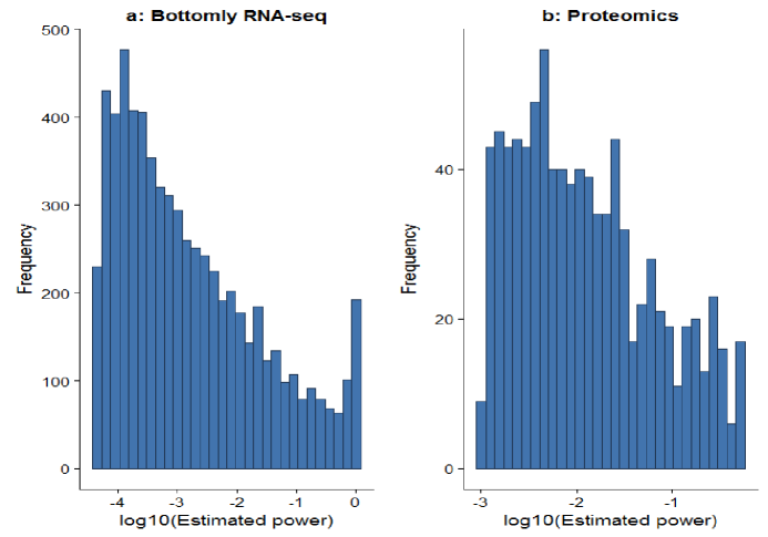
Figure 1: Distribution of Statistical Power in high throughput studies. Post-hoc power estimated across top $m_{1}$ most significant tests in a) the RNA-seq data of Bottomly et al. (2011) and b) the proteomics dataset of Dephoure and Gygi (2012).

3.2 Dilution of group gased weights

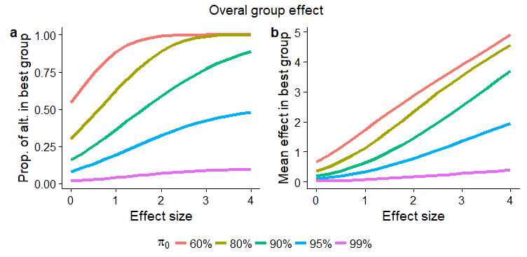
Figure 2: Composition of top group. Simulated test statistics ordered by simulated covariate. The effect sizes for alternative hypothesis tests were generated from a normal distribution with the mean shown on the x-axis. The test statistic and covariate value for each test were generated from a normal distribution with mean equal to the effect size. The left-hand plot shows the proportion of true alternative hypothesis tests in the top-ranked group. The right-hand plot shows the average effect size in the top-ranked group.

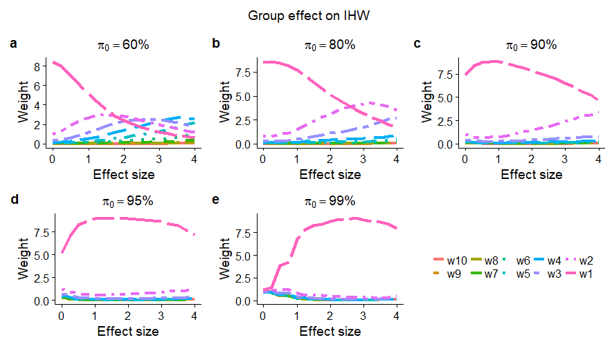
Figure 3: IHW weights. Each curve shows the average weight for one group across 100 replicates. In the legend, $w_{1}-w_{10}$ refers to the weights from the first to the tenth group.

We will demonstrate the dilution effect for group based methods discussed in the Introduction. These methods separate tests into groups by the covariate and then calculate group weights based on group properties. The problem that we now demonstrate is that even the top groups will contain many null tests when true effects are weak and rare. As a result, the group weights will be diluted and are less informative.

As described in the Methods, test statistics and covariate values were generated for $40,000$ hypothesis tests. Tests were sorted into $10$ groups by the covariate, and the proportion of true alternative tests and the average effect size was calculated for the top group (Figure 2).

Ideally, the top group would be comprised primarily of true effects. However, this is only true when the effect sizes are very large, and the proportion of true alternative tests is also large. Over parameter ranges that are typical of most high throughput datasets (for example, the proportion of null hypothesis $\pi_{0}\geq 90\%$ and mean effect size less than one), less than $25\%$ of tests in the top group are true alternative hypothesis. The right-hand panel shows the corresponding average effect size in the top group. For reasonable values of $\pi_{0}$, this is much less than the true average effect size of the data.

Figure 3 shows the weights for each group when the IHW method is applied to data generated in the same manner (see Methods for details). The IHW method is demonstrated because it is the most powerful weighting method currently available. When true alternative effects are weak and rare, only the strongest effects have a chance of being significant. In this case, IHW gives the top group the highest weight and other groups receive weights that are near one or below. The plot shows that the highest weight that the top group receives across all combinations of mean effect size and $\pi_{0}$ is about eight. As $\pi_{0}$ approaches $100\%$ and the average effect decreases below one, the weight of the top group decreases to even lower values. These weights are not large enough to boost power sufficiently for weak effects in high throughput data. We will show in the next section that the CRW method produces stronger weighting for these weak effects.

3.3 Properties of covariate rank weights (CRW)

We explore properties of the rank probabilities and their effect on the CRW weights. Figure 4 shows the rank probability $P(r_{i}\mid\tau)$ of a test from three different approaches: 1) Simulation approach, 2) Exact numerical solution, and 3) Normal approximation of the proposed method. All plots of the simulation suggest nearly perfect alignment with the proposed CRW (exact and approximate) methods. This suggests that the normal approximation (1) is valid.

The values of the weights for different features depend primarily on the value of the rank probability $P(r_{i}=k\mid\tau_{i})$. When the rank for a feature has higher probability, then the feature will be weighted more highly. This figure shows how the probability varies for different combinations of effect sizes for the target test and the remaining tests.

If all effects are null, then ranks have a uniform distribution (Figure 4a). In Fig. 4b, there are $50$ covariates with effect sizes sampled from the $uniform(0,1)$ distribution and $50$ with an effect size of zero. A covariate with effect size at the upper end of this distribution (effect size $=1$) has its rank probability maximized at rank one, but still has a substantial probability of a wide range of lower ranks. This reflects the random variation in covariate statistic values about their expected value. Similarly, a covariate with effect size zero has its rank maximized at rank $100$ but may appear at any rank. In Fig. 4c, the distribution for the alternative hypothesis effects is shifted upwards to $uniform(1,2)$. The distribution for rank probabilities for effect size one now shifts downwards, with rank probability maximized at middle values. In Fig. 4d, a covariate with high effect size relative to other tests has a high probability of being ranked in the top $10$ and low probability of a lower rank.

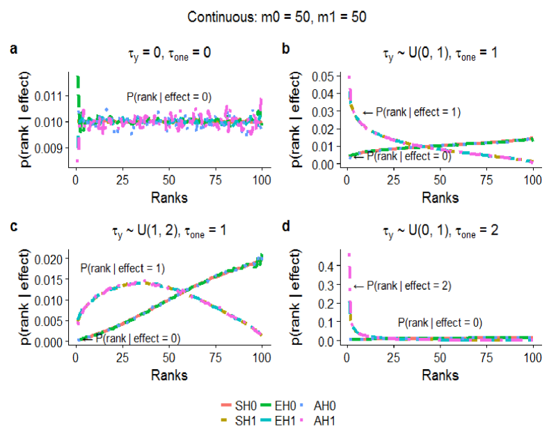
Figure 4: $P(r_{i}=k\mid\tau)$ for continuous effects for three different scenarios: 1) simulation, 2) exact CRW method, and 3) normal approximation of CRW method. We assumed that there are $m=100$ tests of which $m_{0}=50$ are true nulls and $m_{1}=50$ are true effects. The true null tests have mean $0$ and the true effect tests have the distribution $\tau_{y}$ as shown at the top of each plot. Each plot consists of six curves, SH0, SH1, EH0, EH1, AH0, and AH1, where the first letter represents the method (S = simulated, E = exact, and A = approximate), and H0 and H1 represent the hypothesis type. Three curves (SH0, EH0, and AH0) starting from the bottom-left represent $P(r_{i}=k\mid\tau=0)$, and the remaining three curves (SH1, EH1, and AH1) starting from top-left represent $P(r_{i}=k\mid\tau=\tau_{one})$, where $\tau_{one}=\{0,1,2\}$. All the curves show the rank probabilities of a test statistic with effect size either $\tau_{i}=0$ or $\tau_{i}=\tau_{one}$ among all tests. (a) The rank probabilities of a null test when all tests are true nulls. (b) Rank probabilities of a true effect test with effect size $\tau_{one}=1$, when $50$ test statistics are true nulls with effect size $0$, $49$ test statistics have effect size $\tau_{y}\sim uniform(0,1)$, and one test statistic has effect size $\tau_{one}=1$. Similarly, (c) and (d) show the probabilities for different effect size distribution.

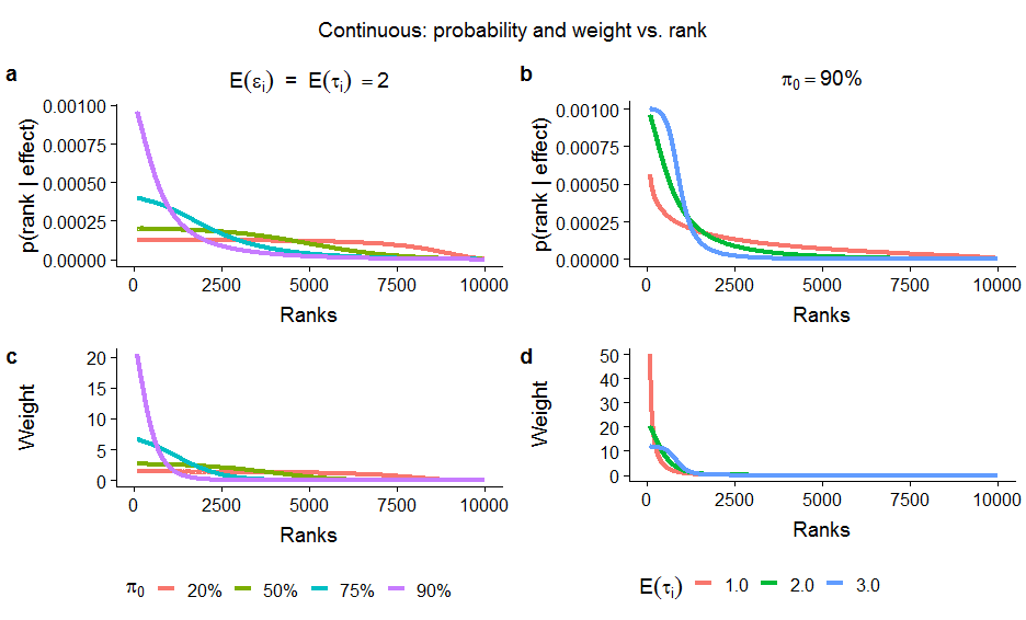
Figure 5: The ranks probabilities, $P(r_{i}=k\mid E(\varepsilon_{i}))$, and the corresponding normalized weights, $w_{i}$, (a) and (c) for different proportions of the true null hypothesis $(\pi_{0})$; and (b) and (d) for different mean covariate-effect $E(\tau_{i})$. The effect size was the same for all true effect tests and equal to the value shown. There were $10,000$ total tests. The curves were smoothed to eliminate random variation due to Monte Carlo integration.

Figure 5 shows ranks probabilities and their corresponding weights. In this figure, all hypothesis tests with true effects have the same covariate effect size, and the rank probability and corresponding weight is shown for one of these tests. In the left-hand plots, the effect size is fixed at a value of $2$, while the proportion of true nulls varies between the different curves. In the right-hand plots, the proportion of true nulls is fixed at $90\%$, and the effect size varies between curves.

As is evident from inspection of the weight equation (4), higher weight is assigned to tests that have a higher rank probability. When the true effect tests are more differentiated from the background, then there is a higher probability of higher rank and thus higher weight for higher ranked tests. This is observed when comparing the different null proportion curves in Fig. 5a and Fig. 5c. When true effect hypothesis tests are rare (e.g., $90\%$ null proportion), then a given true effect hypothesis test is highly likely to be ranked highly and thus it gets a high weight. When there are many true effect hypothesis tests with similar effect sizes (e.g., $20\%$ null proportion), then true effect tests will be spread out over many ranks and thus no rank receives high weight.

Similar trends are seen across varying effect sizes in Fig. 5b and Fig. 5d. When the covariate effect size is high (blue curve), then there is a high probability that all true effect tests will be ranked above all true null tests. In this case, all ranks in the upper $10\%$ are highly likely to be true effect tests and thus all receive the same intermediate size weight. When the covariate effect size is weak (red curve), then null tests are likely to spread over all except the very highest ranks. Thus, the highest ranks get high weights because they are highly differentiated from the background.

This behavior is a highly desirable aspect of the CRW method, i.e., true effects that are rare and low in size will receive the highest boost from weighting. In contrast, such effects will tend to be washed out in group-based approaches to weighting. Comparing Fig. 5 to Fig. 3, we see that the highest ranked tests receive much higher CRW weights than IHW weights (weights of $50+$ with CRW versus $7-8$ in IHW).

In practice, the rank probabilities are calculated by assuming that all alternative hypothesis covariates have equal effect size. This effect size is set equal to the covariate effect size calculated in section 2.4. That is, the covariate effect size corresponding to the mean alternative hypothesis test effect size. This is how the weights are calibrated to the data. The rank probabilities reflect the estimated distribution of effect sizes and the weights vary according to the rank probabilities. Plots of the rank probabilities are given for many other scenarios in the SI.

3.4 Power comparisons of competing methods

Next, we show comparisons of the performance of our method to existing methods of p-value weighting with covariate information. We compared the performance of Benjamini et al. (1997) (BH) with no weighting, Roeder and Wasserman (2009) (RDW), and Independent Hypothesis Weighting (IHW) (Ignatiadis et al., 2016) to our proposed method Covariate Rank Weighing (CRW) in terms of power, FWER, and FDR. To implement the BH and IHW methods, we used p.adjust and ihw function from R software and followed the Benjamini et al. (1997) FDR procedure. To implement the RDW method, we applied the weighting procedures described in Roeder and Wasserman (2009). When the number of the true null hypothesis is low (Figure 6a), the IHW method outperforms CRW if the mean effects size is large. However, for all other situations, CRW equals or outperforms all of the three methods.

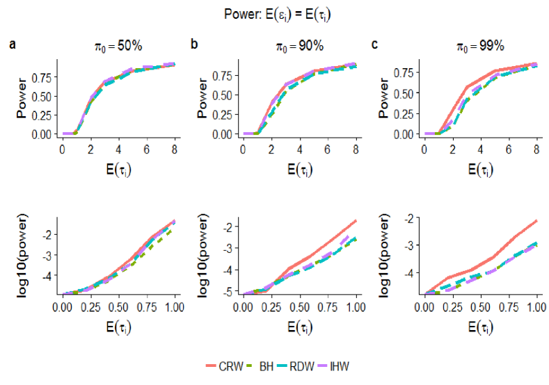
Figure 6: The power of four methods when the mean test-effect $E(\varepsilon_{i})$ is equal to mean covariate-effect $E(\tau_{i})$. Each plot consists of four curves of CRW, BH, RDW, and IHW methods. The first row shows the power for the full range of effect sizes, and the second row shows $log_{10}(power)$ for low effect sizes. The three columns represent the cases of $50\%,90\%,$ and $99\%$ true null hypothesis.

Unlike IHW, CRW computes the weight for each test; therefore, it can more easily detect true effects even though the proportion of the true effects and the effect sizes is relatively low. The relative benefit of CRW over other methods is highest when power is low (bottom row of Figure 6). In this case, it can have a $10$-fold advantage in power over IHW. As shown in section 3.1, very low power is the norm for high-throughput data. Because there are large numbers of tests, the difference between power of, e.g. $0.1\%$ and $1\%$ can make a large difference in the number of discoveries. Consider, for example, a hypothetical genomewide association study which typically might have $500,000$ tests and $5\%$ true effect hypothesis tests. That is, $25,000$ true effect tests. Many of these tests are highly correlated and thus suppose that there are on the order of $5,000$ true underlying effects. Figure 1 shows that typical power for these tests might be in the range $10^{-2}$ to $10^{-3}$. If we assume $5,000$ tests with an average power of $10^{-3}$, then we would expect on the order of $5$ independent significant effects. However, if power can be boosted to $10^{-2}$, then we expect $50$ significant effects.

In the above simulations, we assume that there is a noiseless, linear relationship between the test effect size and the covariate effect size. Next, we show simulations that explore the effect of noise in the test effect-covariate effect relationship. We assume that the test effect is normally distributed around the covariate effect. In the simulation shown (Figure 7), the standard deviation is chosen so that the coefficient of variation (CV) is $1/2$. That is, the standard deviation in test effect size about the covariate effect size is $1/2$ the value of the true covariate effect size. This scenario is typical of high throughput data. There is not a large effect on power for any of the methods and CRW is still the most effective. Further simulations are shown in the SI. All of the methods lose effectiveness as the noise increases, but the relative benefit of CRW decreases with larger noise and CRW eventually becomes inferior. However, this does not occur until the level of noise in the test effect – covariate effect relationship is such that no covariate-based method will be effective.

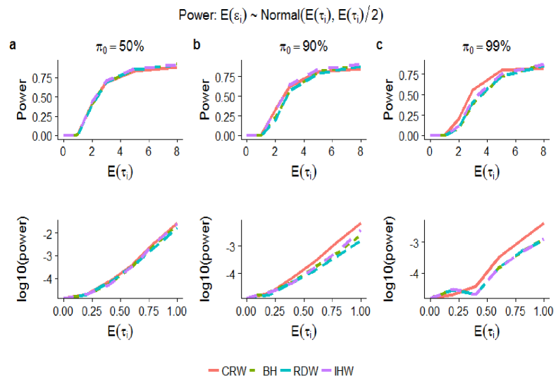
Figure 7: The power for the same parameters described in Fig. 6 except the mean test-effect $E(\varepsilon_{i})$ is not equal to the mean covariate-effect $E(\tau_{i})$; rather $E(\varepsilon_{i})\sim Normal\big{(}E(\tau_{i}),E(\tau_{i})/2\big{)}$, where $CV=1/2$ (for the other cases see SI).

In calculating CRW weights, we assume independence between hypothesis tests. Simulations (see SI) show that correlation between tests does not have a large impact on power, either in absolute terms or comparisons between methods. The exception is for very high correlation $(>80\%)$, at which the performance of IHW increases relative to CRW.

4 Data application

We show two data examples (Figure 8): 1) Bottomly–an RNA-Seq dataset (Bottomly et al., 2011), which has $16,183$ genes and was downloaded from the Recount project Frazee et al. (2011) and 2) Proteomics dataset Dephoure and Gygi (2012) in which differential abundance of $2,666$ proteins was tested.

For the Bottomly data, the estimated proportion of the true null hypothesis was $82\%$. The mean test effect size for true effects was estimated at $1.7$ and $2.2$ for the binary and continuous cases, respectively. The mean covariate effect size for true effect was estimated as $1.2$ for both the binary and continuous cases. The IHW method finds approximately $10\%$ more discoveries than BH, whereas CRW finds greater than $50\%$ more discoveries. Fig. 1a shows that there are many effects with very low power. The ability of CRW to boost the power for weak effects results in a large gain in discoveries.

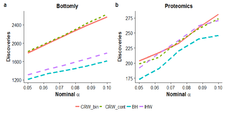
Figure 8: The number of rejected null hypotheses across different significance levels of $\alpha$. Here, CRW_bin = CRW for binary effects, CRW_cont = CRW for continuous effects, BH = Benjamini-Hochberg, and IHW = Independent Hypothesis Weighting methods.

For the Proteomics data, the estimated proportion of the true null hypothesis was $66\%$. The mean test effect size for true effects was estimated as $1.8$ and $2.0$ for the binary and continuous cases, respectively. The mean covariate effect size for true effect was estimated as $0.7$ for both the binary and continuous cases. In this case, IHW and CRW have similar performance, finding about $10\%$ more discoveries than BH. This dataset has conditions that are more favorable for the IHW method relative to CRW: the estimated proportion of true nulls is rather low $(66\%)$ and the power at average effect size is higher than for the Bottomly data.

5 Discussion

The multiple testing problem is fundamental to high throughput data, and the necessary statistical stringency makes detection of features of interest difficult unless their effect size is large. We have shown here for representative data sets that the power to detect most true effects is very low. Unless this problem can be overcome, then the promise of high throughput data may never be realized. Weighted p-values provide a framework for using external information to prioritize the data features that are most likely to be true effects. Many studies (Spjotvoll, 1972; Holm, 1979; Benjamini et al., 1997; Satagopan et al., 2002; Rubin et al., 2006; Roeder et al., 2006; Wasserman and Roeder, 2006; Ionita-Laza et al., 2007; Farcomeni, 2008; Roeder and Wasserman, 2009; Roquain et al., 2009; Bourgon et al., 2010; Dobriban et al., 2015; Kim and Schliekelman, 2015) have proposed methods of p-value weighting and techniques have steadily advanced. However, all existing methods require either 1) difficult to attain knowledge of effect sizes or effect size distributions or 2) grouping tests by the covariate and then estimating properties of the groups. While group-based methods are powerful in many scenarios, their effectiveness may suffer when true features of interest are rare and/or have effect sizes such that power will be low.

Very low statistical power for detection of most features of interest is the norm for high throughput biological data. Furthermore, most tests in most datasets are null. This was observed for both the RNA-seq and proteomics datasets used in this paper, and our experience is that this is typical. The CRW method proposed here assigns an individual weight for each test based on its ranking by the external covariate and gives the strongest weights to true effects when they are weak and rare. It is maximized at the most probable rank for a test that has the average effect size among true effects. Thus, the highest weight tends to be at the center of the distribution of effect sizes for true effects. These weights will not be washed out by group effects. In contrast, in group-based methods like IHW, all covariate-ordered groups will have many null tests, and thus weights will tend to be diluted. We have shown that, as a result, discovery probabilities for weak effects can be increased by as much as $10$-fold relative to the state-of-the-art method IHW.

Although true effects typically form a small proportion of all tests, there are still a large number of them in high throughput datasets. Even though they individually have small power, we expect to detect some because of their large numbers. Thus, the large increase in power relative to other methods that CRW exhibits at low effect sizes can translate into large numbers of extra discoveries even though absolute power is still low.

The CRW method requires knowledge of the probabilistic relationship between covariate rank and test effect size. In this paper, we assume that the covariate follows a normal distribution and then derive an expression for the distribution of covariate rank conditioned on covariate effect size. Performance may suffer when the covariate deviates substantially from normality. The covariate rank-test effect relationship can also be estimated empirically, although the benefit relative to IHW decreases (Hasan, 2017).

Like all covariate-based methods, CRW depends crucially on how well the covariate identifies features of interest. We assume that the test effect size and covariate effect size are related by a linear model. As the relationship gets noisier, the effectiveness of the weights decreases. Simulation results show that power is not highly affected if the coefficient of variation of the test effect around the covariate effects is less than about one. The effectiveness decreases as the coefficient of variation increase beyond one. A fundamental question for all covariate-based methods is whether covariates exist that are able to prioritize promising features sufficiently well to be useful. An important task for future research is to determine good covariates for different data types and how effective those covariates are. Better knowledge of covariates is essential to apply weighting methods effectively and is an important avenue of research for optimization of power in high throughput studies.

Appendix A Appendix

A.1 Proof of theorem 2 - covariate rank

Proof.

Consider a multiple hypothesis testing situation where $m$ tests are being conducted. Each test $i$ has an associated covariate value with effect size $\tau_{i}$. Suppose there are $m_{0}$ null covariate values with $\tau_{i}=0$ and $m_{1}=m-m_{0}$ true alternative covariate values with $\tau_{i}>0$. Let, $x_{1},\ldots,x_{m_{0}}$ be the covariate values for which the null hypothesis is true and $y_{1},\ldots,y_{m_{1}}$ be the covariate values for which the alternative hypothesis is true, and also consider a covariate value $t$. Our goal is to find the distribution for the rank of the covariate value $t$ among the other covariates. Let $k_{0}-1$ and $k_{1}-1$ refer to the number of success, i.e., the number of covariates greater than $t$ among the null and alternative covariates, respectively. Define, $I_{j}$ and $I_{l}$ as follows

$$I_{j}=\begin{cases}1,&\text{if }X_{j}>t\\ 0,&\text{otherwise}\end{cases};\ j=1,\ldots,m_{0}$$

and

$$I_{l}=\begin{cases}1,&\text{if }Y_{l}>t\\ 0,&\text{otherwise}\end{cases};\ l=1,\ldots,m_{1}.$$

Take $S_{0}=\sum_{j=1}^{m_{0}}I_{j}$, then $S_{0}+1$ will give the rank of $t$ among the null covariates. $I_{j}$ is a binary random variable, and assuming independence among the covariates, the number of covariates exceeding $t$ follows a binomial distribution with $m_{0}$ trials and success probability $P(X_{j}>t)$. $P(X_{j}>t)$ can be computed as $P(X_{j}>t)=1-P(X_{j}<t)=1-F_{0}(t)$, where $F_{0}(.)$ is the cumulative density function of $X_{j}$ under the null model. For simplicity, we will denote it $F_{0}$. Thus, if $k_{0}$ is the rank of $t$ denoted by a random variable $r_{0j}$, then

$$P(r_{0j}=k_{0}\mid t)=\binom{m_{0}}{k_{0}-1}(1-F_{0})^{k_{0}-1}F_{0}^{m_{0}-(k_{0}-1)};\ 1\leq k_{0}\leq m_{0}.$$

Similarly, for the alternative hypotheses we have $S_{1}=\sum_{l=1}^{m_{1}}I_{l}$; therefore, the probability of success is $P(Y_{l}>t)=1-P(Y_{l}<t)=1-F_{1}(t)=1-\int F_{1}(t,\tau_{l})f(\tau_{l})d\tau_{l}$. $F_{1}(t)$ is the probability of a randomly chosen covariate statistic exceeding $t$. This depends on the effect size $\tau_{l}$. This effect size is unknown and thus we integrate over possible values. $F_{1}(t,\tau_{l})$ refers to the cumulative density function of $Y_{l}$, with $\tau_{l}$ known. We will denote $P(Y_{l}<t)$ as $F_{1}$. Thus, if $k_{1}$ is the rank of $t$ denoted by a random variable $r_{1l}$, then

$$P(r_{1l}=k_{1}\mid t)=\binom{m_{1}}{k_{1}-1}(1-F_{1})^{k_{1}-1}F_{1}^{m_{1}-(k_{1}-1)};\ 1\leq k_{1}\leq m_{1}.$$

In practice, we do not know $m_{0}$ and $m_{1}$. These parameters can be estimated by the method of Storey and Tibshirani (2003).

Our goal is to obtain rank $k$ under both the null and alternative models, simultaneously, for a random covariate $t$. If the rank of $t$ is $k$, then there are $k-1$ covariates that are higher and $m-k$ covariates that are lower than the covariate $t$, assuming that $t$ is counted as one of the $m$ covariates. Let us suppose a random variable $r_{i}$ refers to the rank of $t$ among all (null and alternative) covariate values simultaneously. Then

$$P(r_{i}=k\mid\tau_{i})=P(r_{0j}+r_{1l}-1=k\mid\tau_{i}),$$

where $i=1,\ldots,m;\ 0\leq k\leq m$; and $m_{0}+m_{1}=m$. This is a joint distribution of $r_{0j}$ and $r_{1l}$. Thus, by applying convolution for the discrete case, we have

$$P(r_{i}=k\mid\tau_{i})=\frac{\sum_{k_{0}=1}^{k}P(r_{1l}+r_{0j}=k+1,\tau_{i},r_{0j}=k_{0})}{p(\tau_{i})}.$$ (9)

Up to this point $t$ has been assumed to be a fixed value. Now, we let $t$ vary with distribution $P(t\mid\tau_{i})$. Incorporating this into (9) produces

$$P(r_{i}=k\mid\tau_{i})=\sum_{k_{0}=1}^{k}\int_{t}P(r_{1i}=k-k_{0}+1\mid\tau_{i},t)P(r_{0i}=k_{0}\mid\tau_{i},t)P(t\mid\tau_{i})dt.$$ (10)

If $t$ is one of the $m_{0}$ null covariates, and we want to compute $P(r_{0i}=k_{0}\mid\tau_{i},t)$, then the number of null trials in the binomial is $m_{0}-1$ and the number of alternative trials is $m_{1}$. If $t$ is one of the $m_{1}$ alternative covariates, then the number of null trials is $m_{0}$ and the number of alternative trials is $m_{1}-1$. Similar arguments hold for calculating $P(r_{1i}=k-k_{0}+1\mid\tau_{i},t)$. Therefore,

$$P(r_{1i}=k-k_{0}+1\mid\tau_{i},t)=\begin{cases}\binom{m_{1}}{k-k_{0}}(1-F_{1})^{k-k_{0}}F_{1}^{m_{1}-(k-k_{0})},&\text{if }\tau_{i}=0\\ \binom{m_{1}-1}{k-k_{0}}(1-F_{1})^{k-k_{0}}F_{1}^{(m_{1}-1)-(k-k_{0})},&\text{if }\tau_{i}>0\end{cases},$$

and

$$P(r_{0i}=k_{0}\mid\tau_{i},t)=\begin{cases}\binom{m_{0}-1}{k_{0}-1}(1-F_{0})^{k_{0}-1}F_{0}^{m_{0}-k_{0}},&\text{if }\tau_{i}=0\\ \binom{m_{0}}{k_{0}-1}(1-F_{0})^{k_{0}-1}F_{0}^{m_{0}-(k_{0}-1)},&\text{if }\tau_{i}>0\end{cases}.$$

The expression $P(r_{i}=k\mid\tau_{i})$ is, in fact, the required probability of rank of the covariate given the effect size. Since $P(t\mid\tau_{i})$ is the probability density function of $t$, (10) can be simplified in terms of expectation ($E_{T}$) over the random variable $t$ as

$$P(r_{i}=k\mid\tau_{i})=\sum_{k_{0}=1}^{k}E_{T}\Big{[}P(r_{1i}=k-k_{0}+1\mid\tau_{i},t)P(r_{0i}=k_{0}\mid\tau_{i},t)\Big{]}$$

This finishes the proof. ∎

A.2 Proof of proposition 1 - covariate rank is the expected value of the normal PDF

Proof.

If $\tau_{i}=0,$ then from (10) $P(r_{i}=k\mid\tau_{i})$ can be written as

$$P(r_{i}=k\mid\tau_{i})=\sum_{k_{0}=1}^{k}E_{T}\bigg{[}\binom{m_{0}-1}{k_{0}-1}(1-F_{0})^{k_{0}-1}F_{0}^{m_{0}-k_{0}}.\binom{m_{1}}{k-k_{0}}(1-F_{1})^{k-k_{0}}F_{1}^{m_{1}-(k-k_{0})}\bigg{]}.$$

Equivalently,

$$P(r_{i}=k\mid\tau_{i})=E_{T}\sum_{k_{0}=1}^{k}\bigg{[}\binom{m_{0}-1}{k_{0}-1}(1-F_{0})^{k_{0}-1}F_{0}^{m_{0}-k_{0}}.\binom{m_{1}}{k-k_{0}}(1-F_{1})^{k-k_{0}}F_{1}^{m_{1}-(k-k_{0})}\bigg{]}.$$

Suppose we have two Binomial random variables $X=k_{1}-1\sim Binom(m_{1},1-F_{1})$ and $Y=k_{0}-1\sim Binom(m_{0}-1,1-F_{0})$; and we want to obtain pmf of $Z=X+Y$. Then

$$\begin{split}P(Z=k-1)&=P(X+Y=k-1)\\ &=P(X=k-1-Y)\\ &=\sum_{k_{0}-1=0}^{k-1}P(X=k-k_{0})P(Y=k_{0}-1)\\ &=\sum_{k_{0}-1=0}^{k-1}\binom{m_{1}}{k-k_{0}}(1-F_{1})^{k-k_{0}}F_{1}^{m_{1}-(k-k_{0})}.\binom{m_{0}-1}{k_{0}-1}(1-F_{0})^{k_{0}-1}F_{0}^{m_{0}-k_{0}}.\end{split}$$

Therefore,

$$P(r_{i}=k\mid\tau_{i})=E_{T}P(Z=k-1)=E_{T}P(Z+1=k),$$

where $Z$ is a sum of two independent binomial random variables. Thus, the PDF of $Z+1$ can be approximated by normal PDF with mean $=E(X+Y+1)$ and variance $=var(X+Y+1)$. Similarly, we can also obtain an approximation when $\tau_{i}>0$. ∎

References

- Benjamini and Hochberg (1995) Benjamini, Y. and Y. Hochberg (1995). Controlling the false discovery rate: a practical and powerful approach to multiple testing. Journal of the royal statistical society. Series B (Methodological), 289–300.
- Benjamini et al. (1997) Benjamini, Y., Y. Hochberg, and Y. Kling (1997). False discovery rate control in multiple hypotheses testing using dependent test statistics. Research Paper 97 1.
- Bottomly et al. (2011) Bottomly, D., N. A. Walter, J. E. Hunter, P. Darakjian, S. Kawane, K. J. Buck, R. P. Searles, M. Mooney, S. K. McWeeney, and R. Hitzemann (2011). Evaluating gene expression in c57bl/6j and dba/2j mouse striatum using rna-seq and microarrays. PloS one 6(3), e17820.
- Bourgon et al. (2010) Bourgon, R., R. Gentleman, and W. Huber (2010). Independent filtering increases detection power for high-throughput experiments. Proceedings of the National Academy of Sciences 107(21), 9546–9551.
- Dephoure and Gygi (2012) Dephoure, N. and S. P. Gygi (2012). Hyperplexing: a method for higher-order multiplexed quantitative proteomics provides a map of the dynamic response to rapamycin in yeast. Sci. Signal. 5(217), rs2–rs2.
- Dobriban et al. (2015) Dobriban, E., K. Fortney, S. K. Kim, and A. B. Owen (2015). Optimal multiple testing under a gaussian prior on the effect sizes. Biometrika 102(4), 753–766.
- Farcomeni (2008) Farcomeni, A. (2008). A review of modern multiple hypothesis testing, with particular attention to the false discovery proportion. Statistical methods in medical research 17(4), 347–388.
- Frazee et al. (2011) Frazee, A. C., B. Langmead, and J. T. Leek (2011). Recount: a multi-experiment resource of analysis-ready rna-seq gene count datasets. BMC bioinformatics 12(1), 449.
- Genovese et al. (2006) Genovese, C. R., K. Roeder, and L. Wasserman (2006). False discovery control with p-value weighting. Biometrika 93(3), 509–524.
- Hasan (2017) Hasan, M. S. (2017). Optimal p-value weighting with independent information. arXiv preprint arXiv:1712.07197.
- Holm (1979) Holm, S. (1979). A simple sequentially rejective multiple test procedure. Scandinavian journal of statistics, 65–70.
- Ignatiadis et al. (2016) Ignatiadis, N., B. Klaus, J. B. Zaugg, and W. Huber (2016). Data-driven hypothesis weighting increases detection power in genome-scale multiple testing. Nature methods.
- Ionita-Laza et al. (2007) Ionita-Laza, I., M. B. McQueen, N. M. Laird, and C. Lange (2007). Genomewide weighted hypothesis testing in family-based association studies, with an application to a 100k scan. The American Journal of Human Genetics 81(3), 607–614.
- Kim and Schliekelman (2015) Kim, S. and P. Schliekelman (2015). Prioritizing hypothesis tests for high throughput data. Bioinformatics, btv608.
- Roeder et al. (2006) Roeder, K., S.-A. Bacanu, L. Wasserman, and B. Devlin (2006). Using linkage genome scans to improve power of association in genome scans. The American Journal of Human Genetics 78(2), 243–252.
- Roeder and Wasserman (2009) Roeder, K. and L. Wasserman (2009). Genome-wide significance levels and weighted hypothesis testing. Statistical science: a review journal of the Institute of Mathematical Statistics 24(4), 398.
- Roquain et al. (2009) Roquain, E., M. A. Van De Wiel, et al. (2009). Optimal weighting for false discovery rate control. Electronic journal of statistics 3, 678–711.
- Rosenthal and Rubin (1983) Rosenthal, R. and D. B. Rubin (1983). Ensemble-adjusted p values. Psychological Bulletin 94(3), 540.
- Rubin et al. (2006) Rubin, D., S. Dudoit, and M. Van der Laan (2006). A method to increase the power of multiple testing procedures through sample splitting. Statistical Applications in Genetics and Molecular Biology 5(1).
- Satagopan et al. (2002) Satagopan, J. M., D. A. Verbel, E. Venkatraman, K. E. Offit, and C. B. Begg (2002). Two-stage designs for gene–disease association studies. Biometrics 58(1), 163–170.
- Spjotvoll (1972) Spjotvoll, E. (1972). On the optimality of some multiple comparison procedures. The Annals of Mathematical Statistics, 398–411.
- Storey and Tibshirani (2003) Storey, J. D. and R. Tibshirani (2003). Statistical significance for genomewide studies. Proceedings of the National Academy of Sciences 100(16), 9440–9445.
- Wasserman and Roeder (2006) Wasserman, L. and K. Roeder (2006). Weighted hypothesis testing. arXiv preprint math/0604172.
- Westfall et al. (2004) Westfall, P. H., S. Kropf, L. Finos, et al. (2004). Weighted fwe-controlling methods in high-dimensional situations. In Recent developments in multiple comparison procedures, pp. 143–154. Institute of Mathematical Statistics.