Unimon qubit

Abstract

Superconducting qubits[1, 2] are one of the most promising candidates to implement quantum computers, with projected applications in physics simulations[3], optimization[4], machine learning[5], and chemistry[6]. The superiority of superconducting quantum computers over any classical device in simulating random but well-determined quantum circuits has already been shown in two independent experiments[7, 8] and important steps have been taken in quantum error correction[9, 10, 11]. However, the currently wide-spread qubit designs[12, 13, 14, 15, 16] do not yet provide high enough performance to enable practical applications or efficient scaling of logical qubits owing to one or several following issues: sensitivity to charge or flux noise leading to decoherence, too weak non-linearity preventing fast operations, undesirably dense excitation spectrum, or complicated design vulnerable to parasitic capacitance. Here, we introduce and demonstrate a superconducting-qubit type, the unimon, which combines the desired properties of high non-linearity, full insensitivity to dc charge noise, insensitivity to flux noise, and a simple structure consisting only of a single Josephson junction in a resonator. We measure the qubit frequency, $\omega_{01}/(2\pi)$, and anharmonicity $\alpha$ over the full dc-flux range and observe, in agreement with our quantum models, that the qubit anharmonicity is greatly enhanced at the optimal operation point, yielding, for example, 99.9% and 99.8% fidelity for 13-ns single-qubit gates on two qubits with $(\omega_{01},\alpha)=(4.49\leavevmode\nobreak\ \mathrm{GHz},434\leavevmode\nobreak\ \mathrm{MHz})\times 2\pi$ and $(3.55\leavevmode\nobreak\ \mathrm{GHz},744\leavevmode\nobreak\ \mathrm{MHz})\times 2\pi$, respectively. The energy relaxation time $T_{1}\lesssim 10\leavevmode\nobreak\ \mu\mathrm{s}$ is stable for hours and seems to be limited by dielectric losses. Thus, future improvements of the design, materials, and gate time may promote the unimon to break the 99.99% fidelity target for efficient quantum error correction and possible quantum advantage with noisy systems.

Introduction

Even though quantum supremacy has already been reached with superconducting qubits in specific computational tasks[7, 8], the current quantum computers still suffer from errors owing to noise. In this so-called noisy intermediate-scale quantum (NISQ) era[17], the complexity of the implementable quantum computations[18] is mostly limited by errors in single- and two-qubit quantum gates. Crudely speaking, the process fidelity of implementing a $d$-deep $n$-qubit logic circuit with gate fidelity $F$ is $F^{dn}$. Thus, to succeed roughly half of the time in a 100-qubit circuit of depth five, one needs at least 99.9% gate fidelity. In practice, the number of qubits and especially the gate depth required for useful NISQ advantage is likely higher, leading to a fidelity target of 99.99% for all quantum gates, not yet demonstrated in any superconducting quantum computer.

The effect of gate errors can be reduced to some extent using error mitigation[19, 20] or in principle, completely using quantum error correction[21]. Surface codes[22, 23] are regarded as some of the most compelling error correction codes for superconducting qubits owing to the two-dimensional topology of the qubit register and their favorable fidelity threshold of roughly 99% which has been reached with superconducting transmon qubits already in 2014[24]. Despite the recent major developments in implementing distance-two and -three surface codes on superconducting quantum processors[25, 26, 27, 28], the gate and readout fidelities of superconducting qubits need to be improved further, preferably above 99.99%, to enable efficient quantum error correction with a reasonable qubit count.

Currently, most of the superconducting multi-qubit processors utilize transmon qubits[7, 29, 25, 30] that can be reproducibly fabricated[29] and have coherence times up to several hundred microseconds[31, 32], leading to record average gate fidelities of 99.98% for single-qubit gates[33] and 99.8%–99.9% for two-qubit gates[34]. The transmon was derived from the charge qubit[35] by adding a shunt capacitor in parallel with a Josephson junction, with the result of exponentially suppressing the susceptibility of its transition frequency to charge noise. However, the large shunt capacitance results in a relatively low anharmonicity of 200–300 MHz corresponding to only 5% of the typical qubit frequency[12, 36]. This limits the speed of quantum gates that can be implemented with transmons since leakage errors to the states beyond the computational subspace need to be suppressed[33, 37]. Similarly, the low anharmonicity also limits the readout speed of transmon qubits, and a high-power readout tone can even excite the transmon to unconfined states beyond the cosine potential[38]. A higher anharmonicity is preferred to speed up the qubit operations and to allow for higher fidelities limited by the finite coherence time.

Hence, there is an urgent need to find new superconducting qubit types that increase the anharmonicity–coherence-time product. Recently, major progress has been made in the development of fluxonium qubits, one of the most compelling alternatives to transmons thanks to their high anharmonicity and long relaxation and coherence times[39, 40, 41]. In a fluxonium qubit, a small Josephson junction is shunted by a superinductor implemented by an array of large Josephson junctions[39, 41, 13], a granular aluminum wire[42], a nanowire with a high kinetic inductance[43], or a geometric superinductor[44]. The superinductor in the fluxonium ensures that the dephasing and relaxation rates arising from flux noise are reduced, in addition to which all the levels of a fluxonium are fully protected against dephasing arising from low-frequency charge noise. It is possible to add a large shunt capacitor into the fluxonium in order to create a so-called heavy fluxonium[45, 41], in which the transition matrix element between the ground state and the first excited state can be suppressed to enhance the relaxation time up to the millisecond regime[45]. However, special techniques are required to control, readout, and reset these high-coherence fluxonium qubits due to their low frequency and small transition matrix elements in the vicinity of the half flux quantum operation point[41]. Furthermore, it is not possible to achieve protection against both relaxation and dephasing due to flux noise at a single operation point. Parasitic capacitances in the superinductor may also provide a challenge for the reproducible fabrication of fluxonium qubits and result in parasitic modes.

By reducing the total inductance of the junction array in the fluxonium, it is possible to implement a plasmonium qubit[46] operated at zero flux or a quarton qubit[16] operated at the half-flux-quantum point, both of which have a small size and a high anharmonicity compared with the transmon and a sufficient protection against charge noise in comparison to current coherence times. On the other hand, an enhancement of the superinductance converts the fluxonium into a so-called quasicharge qubit[14], the charge-basis eigenstates of which resemble those of the early charge qubits while retaining the protection against charge noise. Other qubits protected against some sources of relaxation and dephasing include the $0-\pi$ qubit[15], bifluxon[47], and a qubit protected by two-Cooper-pair tunneling[48]. The $0-\pi$ qubit is protected against both relaxation and dephasing arising from charge and flux noise thanks to its topological features, which unfortunately renders the qubit challenging to operate and its circuit relatively complicated and hence vulnerable to parasitic capacitance. Despite this great progress in fluxonium and protected qubits, they have still not shown broad superiority to the transmons. The race for the new improved mainstream superconducting qubit continues.

In this work, we introduce and demonstrate a novel superconducting qubit, the unimon, that consists of a single Josephson junction shunted by a linear inductor and a capacitor in a largely unexplored parameter regime where the inductive energy is mostly cancelled by the Josephson energy leading to high anharmonicity while being fully resilient against low-frequency charge noise and partially protected from flux noise (Fig. 1). We measure the unimon frequency and anharmonicity in a broad range of flux biases and find a very good agreement with first-principles models (Fig. 2), even for five different qubits (Fig. 3a). According to our experimental data, the energy relaxation time seems to be limited by dielectric losses (Fig. 3b), and the coherence time can be protected from flux noise at a flux-insensitive sweet spot (Fig. 3c). Importantly, we observe that the single-qubit gate fidelity progressively increases with decreasing gate duration, and is stable for hours at 99.9% for a 13-ns gate duration (Fig. 4), demonstrating that the unimon is a promising candidate for a new mainstream superconducting qubit.

Unimon

In practice, we implement the unimon in a simple superconducting circuit by integrating a single Josephson junction into the center conductor of a superconducting coplanar-waveguide (CPW) resonator grounded at both ends (Fig. 1b). There are no charge islands in the circuit, and hence the junction is inductively shunted. In addition to the very recent fluxonium qubit utilizing a geometric superinductance[44], the unimon is the only superconducting qubit with the Josephson junction shunted by a geometric inductance that provides complete protection against low-frequency charge noise. Due to the non-linearity of the Josephson junction, the normal modes of the resonator with a non-zero current across the junction are converted into anharmonic oscillators that can be used as qubits. In this work, we use the lowest anharmonic mode as the qubit since it has the highest anharmonicity.

The frequency of each anharmonic mode can be controlled by applying external fluxes $\Phi_{\mathrm{ext,1}}$ and $\Phi_{\mathrm{ext,2}}$ through the two superconducting loops of the resonator structure as illustrated in Fig. 1b. The unimon is partially protected against flux noise thanks to its gradiometric structure, which signifies that the superconducting phase across the Josephson junction is dependent on the half difference of the applied external magnetic fluxes $\Phi_{\mathrm{diff}}=(\Phi_{\mathrm{ext,2}}-\Phi_{\mathrm{ext,1}})/2$. Interestingly, the anharmonicity of the unimon is maximized at a flux-insensitive sweet spot, at which the qubit frequency is unaffected by the external flux difference to the first order. This optimal operation point is obtained at $\Phi_{\mathrm{diff}}=\Phi_{0}/2$ modulo integer flux quanta $\Phi_{0}=h/(2e)\approx 2.067\times 10^{-15}$ Wb, where $h$ is the Planck constant and $e$ is the elementary charge.

Using the distributed-element circuit model shown in Fig. 1c, the effective Hamiltonian of the qubit mode $m$ can be written (model 1 in Methods) as

$$\hat{H}_{m}=4E_{C,m}(\varphi_{0})\hat{n}_{m}^{2}+\frac{1}{2}E_{L,m}(\varphi_{0})\hat{\varphi}_{m}^{2}+E_{L}\hat{\varphi}_{m}\left(\frac{2\pi\Phi_{\mathrm{diff}}}{\Phi_{0}}-\varphi_{0}\right)-E_{\mathrm{J}}\cos(\hat{\varphi}_{m}-\varphi_{0}),$$ (1)

where $\varphi_{0}$ is the Josephson phase of a dc current across the junction, $E_{C,m}(\varphi_{0})$ is the capacitive energy of the qubit mode, $E_{L,m}(\varphi_{0})$ is the inductive energy of the qubit mode, $E_{L}$ is the inductive energy of the dc current, $E_{\mathrm{J}}$ is the Josephson energy, and $\hat{n}_{m}$ and $\hat{\varphi}_{m}$ are the Cooper pair number and phase operators corresponding to the qubit mode $m$ and satisfying $[\hat{\varphi}_{m},\hat{n}_{m}]=\mathrm{i}$ with $\mathrm{i}$ being the imaginary unit. Note that $\varphi_{0}$ is treated as a classical variable depending on the flux bias $\Phi_{\mathrm{diff}}$ according to a transcendental equation such that $2\pi\Phi_{\mathrm{diff}}/\Phi_{0}-\varphi_{0}$ is periodic in $\Phi_{\mathrm{diff}}$. (See Extended Data Fig. 1 for solutions of equation (1).)

At the sweet spot $\Phi_{\mathrm{diff}}=\Phi_{0}/2$, the dc phase equals $\varphi_{0}=\pi$ and the Hamiltonian of the unimon reduces to

$$\hat{H}_{m}=4E_{C,m}(\pi)\hat{n}_{m}^{2}+\frac{1}{2}E_{L,m}(\pi)\hat{\varphi}_{m}^{2}+E_{\mathrm{J}}\cos(\hat{\varphi}_{m}),$$ (2)

where we assume that $E_{\mathrm{J}}\leq E_{L}$. Strikingly, this Hamiltonian is exactly analogous to a simple mechanical system visualized in Fig. 1d, in which an inverted pendulum is attached to a twisting beam. In this analogy, the gravitational potential energy of the pendulum corresponds to the cosine-shaped Josephson potential, the harmonic potential energy associated with the twisting of the beam corresponds to the inductive energy of the unimon, and the moment of inertia of the pendulum is analogous to the capacitance in the unimon. Furthermore, the twist angle $\varphi$ is analogous to the superconducting phase difference $\hat{\varphi}_{m}$ of the qubit mode across the Josephson junction. This mechanical analogue provides great intuition to the physics of the unimon.

In this work, we employ the parameter regime $E_{\mathrm{J}}\lesssim E_{L,m}(\pi)\approx E_{L}$ to provide a large anharmonicity without any superinductors. As a result, it is instructive to use the Taylor expansion of the cosine and write the sweet-spot Hamiltonian of the unimon in Eq. (2) as

$$\hat{H}_{m}=4E_{C,m}(\pi)\hat{n}_{m}^{2}+\frac{E_{L,m}(\pi)-E_{\mathrm{J}}}{2}\hat{\varphi}_{m}^{2}+\frac{E_{\mathrm{J}}}{24}\hat{\varphi}_{m}^{4}+\mathcal{O}(\hat{\varphi}_{m}^{6}).$$ (3)

The quadratic term proportional to $\propto(E_{L,m}(\pi)-E_{\mathrm{J}})$ is mostly cancelled in the unimon regime, which emphasizes the high-order terms in the potential energy and hence increases the anharmonicity of the qubit. This cancellation bears resemblance to the quarton qubit[16] with the distinctive difference that the quadratic inductive energy of a quarton qubit is only an approximation for the actual potential energy function of a short Josephson junction array, as a result of which the quarton circuit is not fully protected against low-frequency charge noise unlike the unimon.

To experimentally demonstrate the unimon qubit, we design and fabricate samples, each of which consists of three unimon qubits as illustrated in Fig. 1e. We use niobium as the superconducting material apart from the Josephson junctions, in which the superconducting leads are fabricated using aluminum (see Sample Fabrication in Methods). The CPW structure of the unimon is designed for characteristic impedance $Z=100$ $\Omega$ to reduce the total capacitance of the unimon in comparison to a standard 50-$\Omega$ resonator. Each qubit is capacitively coupled to an individual drive line that enables single-qubit rotations in a similar manner as for conventional transmon qubits by applying attenuated microwave pulses along the drive line as illustrated in the simplified schematic of the experimental setup in Fig. 1f (see also Extended Data Fig. 2). All experiments are carried out at 10-mK base temperature of a pulse-tube-cooled dilution refrigerator. Furthermore, each qubit is capacitively coupled to a readout resonator using a U-shaped capacitor in order to enable dispersive qubit state measurements[49, 50] similar to those conventionally used with transmon qubits[27]. The frequency of the qubits is tuned by applying a current through an external coil attached to the sample holder such that one flux quantum $\Phi_{0}$ approximately corresponds to 10 $\mu$A.

Results

We experimentally study five unimon qubits, A–E, on two different chips. In all of the qubits, the geometry of the CPW resonator is similar, but the qubits have different Josephson energies $E_{\mathrm{J}}$ corresponding to different amounts of cancellation $\propto(E_{L,m}(\pi)-E_{\mathrm{J}})$ of the quadratic potential energy terms. Furthermore, the coupling capacitance between a qubit and its readout resonator has been designed to be different on the two chips. We present the main measured properties for all of the five qubits in Extended Data Tables 1 and 2. Design targets of the parameter values are provided in Extended Data Table 3. The results discussed below are obtained from qubit B unless otherwise stated.

In Fig. 2a, we show the microwave response of the readout resonator as a function of the flux bias $\Phi_{\mathrm{diff}}$ through the unimon loops. We observe that the frequency of the readout resonator changes periodically, as expected, since a change of flux by a flux quantum has no observable effect on the full circuit Hamiltonian in equation (1). Furthermore, the frequency of the readout resonator exhibits an avoided crossing where the first transition frequency of the bare qubit $f_{01}=\omega_{01}/(2\pi)$ crosses the bare resonator frequency. By fitting our theoretical model of the coupled unimon-resonator system (see Methods and Supplementary Note II) to the experimental data of the avoided crossing shown in Fig. 2b, we estimate that the coupling capacitance between the qubit and the readout resonator is $C_{\mathrm{g}}=10.0$ fF in good agreement with the design value of 10.4 fF obtained from our classical electromagnetic simulations.

Figure 2(c) shows the results of a two-tone experiment to map the qubit frequency spectrum (Methods). We observe that the single-photon transition between the ground state $|0\rangle$ and the first excited state $|1\rangle$ has a minimum frequency of $f_{01}=4.488$ GHz at $\Phi_{\mathrm{diff}}/\Phi_{0}=-0.5$ and a maximum frequency of $f_{01}=9.05$ GHz at $\Phi_{\mathrm{diff}}=0$. The two-photon transition $|0\rangle\leftrightarrow|2\rangle$ is also clearly visible, which allows us to verify that the anharmonicity $\alpha/(2\pi)=f_{12}-f_{01}$ of the qubit is enhanced at the sweet spot $\Phi_{\mathrm{diff}}/\Phi_{0}=-0.5$ to $\alpha/(2\pi)=434$ MHz. (See Extended Data Fig. 3 for an alternative agreeing way to measure the anharmonicity.)

Figure 2(c) presents fits to the experimental transition frequencies $f_{01}$ and $f_{02}/2$ based on two theoretical models of the circuit Hamiltonian, the first of which corresponds to Eq. (1) (model 1 in Methods) and the second of which is based on a path integral approach that does not require the dc phase $\varphi_{0}$ to be treated as a classical variable (model 2 in Methods). The fits agree very well with the experimental transition frequencies, especially near the sweet spots $\Phi_{\mathrm{diff}}=0$ and $\Phi_{\mathrm{diff}}/\Phi_{0}=-0.5$. Importantly, this good agreement with the models and the qubit frequency and anharmonicity is obtained with only three fitting parameters in a broad range of flux biases, and hence confirms our interpretation of the unimon physics (Fig. 1d) and justifies the use of the models for reliable predictions of promising parameter regimes. According to the fits of model 1 (model 2), the capacitance and inductance per unit length of the unimon have a value of $C_{l}=87.1$ pF/m ($C_{l}=79.8$ pF/m) and $L_{l}=0.821$ $\mu$H/m ($L_{l}=0.893$ $\mu$H/m), respectively, in good agreement with the design values of $C_{l}=83$ pF/m and $L_{l}=0.83$ $\mu$H/m.

The measured sweet-spot anharmonicities of the five qubits are shown in Fig. 3a as functions of the Josephson energy $E_{\mathrm{J}}$ that is estimated by fitting the models 1 and 2 to the qubit spectroscopy data as in Figure 2(c). The measured anharmonicities are slightly lower, but very close to the values predicted by the two theoretical models. The qubits A and B exhibit the highest anharmonicities of $\alpha/(2\pi)=744$ MHz and $434$ MHz, respectively, as a result of the largest cancellation between the inductive energy $E_{L,m}$ and the Josephson energy $E_{\mathrm{J}}$. Importantly, the anharmonicity of the qubits A and B is significantly higher than that of typical transmon qubits, 200–300 MHz[36]. Furthermore, the measured anharmonicities greatly exceed the capacitive energy $E_{C,m}$ of the qubit mode unlike for transmons.

To study the mechanisms determining the energy relaxation time $T_{1}$ of the unimon, we measure $T_{1}$ as a function of the qubit frequency as shown in Fig. 3b (see also Extended Data Figs. 4 and 5). At the $\Phi_{\mathrm{diff}}=\Phi_{0}/2$ sweet spot, we find $T_{1}\approx 8.6$ $\mu$s, whereas $T_{1}\approx 4.6$ $\mu$s at $\Phi_{\mathrm{diff}}=0$. Between these flux sweet spots, the relaxation time attains a minimum in a frequency range close to the frequency of the readout resonator $f_{\mathrm{r}}=6.198$ GHz. This behaviour of $T_{1}$ can be reasonably explained by dielectric losses with an effective quality factor of $Q_{C}\approx 1.7\times 10^{5}$ and Purcell decay through the readout resonator (See Methods and Supplementary Note III). This suggests the qubit energy relaxation to be dominated by dielectric losses at $\Phi_{\mathrm{diff}}=\Phi_{0}/2$. The estimated quality factor of this first unimon qubit is 3–7 times higher than for the other geometric-superinductance qubit[51], but 2–3 times lower than in fluxoniums[41, 13] and an order of magnitude lower than in state-of-the-art transmons[31]. Improvements to design, materials, and fabrication processes are expected to reduce the dielectric losses in future unimon qubits compared with the very first samples presented here.

To characterize the sensitivity of the qubit to flux noise, we measure the Ramsey coherence time $T_{2}^{*}$ and the echo coherence time $T_{2}^{\mathrm{e}}$ with a single echo $\pi$-pulse (Extended Data Fig. 6) as a function of the flux bias $\Phi_{\mathrm{diff}}$. Figure 3(c) shows that $T_{2}^{*}$ and $T_{2}^{\mathrm{e}}$ are both maximized at $\Phi_{\mathrm{diff}}=\Phi_{0}/2$, reaching 3.1 $\mu$s and 9.2 $\mu$s, respectively. Away from the sweet spot, the Ramsey coherence time $T_{2}^{*}$ degrades quickly, but the echo coherence time $T_{2}^{\mathrm{e}}$ stays above 1 $\mu$s even if the qubit frequency is tuned from the sweet spot by over 30 MHz. Assuming that the flux noise is described by a $1/f$ noise model $S_{\Phi_{\mathrm{diff}}}(\omega)=2\pi A_{\Phi_{\mathrm{diff}}}^{2}/\omega$, we estimate a flux noise density of $A_{\Phi_{\mathrm{diff}}}/\sqrt{\textrm{Hz}}=15.0$ $\mu\Phi_{0}/\sqrt{\textrm{Hz}}$ based on the flux dependence of $T_{2}^{\mathrm{e}}$ (Methods). The estimated flux noise density is an order of magnitude greater than in state-of-the-art SQUIDS[52], but an order of magnitude lower than reported for all previous geometric-superinductance qubits[44].

At $\Phi_{\mathrm{diff}}=0$ in contrast, we measure a Ramsey coherence time of $T_{2}^{*}=6.8$ $\mu$s and a $T_{1}$-limited echo coherence time of $T_{2}^{\mathrm{e}}=9.9$ $\mu$s. The dephasing rate is lower here than at $\Phi_{\mathrm{diff}}=-\Phi_{0}/2$ since the qubit frequency is less sensitive to the external flux difference due to lower $|\partial\omega_{01}/\partial\Phi_{\mathrm{diff}}|$. Note that the anharmonicity of the qubit at $\Phi_{\mathrm{diff}}=0$ is only $\alpha/(2\pi)=-58$ MHz, and hence this operation point is not of great interest for implementations of high-fidelity quantum logic.

Next, we demonstrate that the high anharmonicity of the unimon and its protection against charge and flux noise enable us to implement fast high-fidelity single-qubit gates. To this end, we calibrate single-qubit gates of duration $t_{\mathrm{g}}\in[13.3,46.6]$ ns using microwave pulses parametrized according to the derivative removal by adiabatic gate (DRAG) framework[53, 54]. To characterize the average fidelity of gates in the set $\{I,X(\pi/2),Y(\pi/2)\}$, we utilize interleaved randomized benchmarking[55] (Methods). Figure 4(a) shows that we reach a practically coherence-limited fidelity of 99.9% for $I$, $X(\pi/2)$, and $Y(\pi/2)$ gates at 13.3-ns duration. Our electronics limit the shortest gate pulses to 13.3 ns although the anharmonicity should allow for high-fidelity gates down to 5-ns duration corresponding to a gate fidelity of 99.97% with the reported coherence properties.

To study the long-term stability of the gate fidelity, we first calibrate 20-ns single-qubit gates and then conduct repetitive measurements of the average gate fidelity using standard randomized benchmarking[56, 57] without any recalibration between repetitions. Figure 4(b) indicates that the measured gate fidelity is stable over the full period of eight hours with an average fidelity of $99.88\pm 0.02$%, practically coinciding with the coherence limit of 99.89%. This stability can be attributed to the relaxation time $T_{1}$ and the coherence times $T_{2}^{*}$ and $T_{2}^{\mathrm{e}}$ staying practically constant in time as illustrated in Fig.  4c.

Conclusions and outlook

In conclusion, we introduced and demonstrated the unimon qubit that has a relatively high anharmonicity while requiring only a single Josephson junction without any superinductors, and being protected against both low-frequency charge noise and flux noise. The geometric inductance of the unimon has the potential for higher predictability and reproducibility than the junction-array-based superinductors in conventional fluxoniums or in quartons. Thus, the unimon constitutes a promising candidate for achieving single-qubit gate fidelities beyond 99.99% in superconducting qubits with the help of the following future improvements: (i) redesign of the geometry to minimize dielectric losses[58] currently dominating the energy relaxation, (ii) use of recently found low-loss materials[31], and (iii) reduction of the gate duration to values well below 10 ns allowed even by the anharmonicities achieved here. Future unimon research is also needed to study and minimize the various on-chip cross talks, implement two-qubit gates, and to scale up to many-qubit processors. To further reduce the sensitivity of the unimon to flux noise and to scale up the qubit count, it is likely beneficial to reduce the footprint of a single unimon qubit using, e.g., a superconductor with a high kinetic inductance in the coplanar-waveguide resonator. The anharmonicity of the unimon at flux bias $\Phi_{\mathrm{diff}}=\Phi_{0}/2$ has an opposite sign to that of the transmon, which may be helpful to suppress the unwanted residual $ZZ$ interaction with two-qubit-gate schemes that utilize qubits with opposite-sign anharmoncities[59, 60]. The distributed-element nature of the unimon provides further opportunities for implementing a high connectivity and distant couplings in multi-qubit processors. In the future, we also aim to study the utilization of other modes of the unimon circuit, for example, for additional qubits and qubit readout.

References

Methods

Hamiltonian based on a model of coupled normal modes (model 1)
Here, we provide a brief summary of the theoretical model 1 that is used to derive a Hamiltonian for the unimon qubit, starting from the normal modes of the distributed-element circuit illustrated in Fig. 1c. A complete derivation is provided in Supplementary Methods I. In this theoretical model, we extend the approach of Ref.[61] to model phase-biased Josephson junctions in distributed-element resonators in the presence of an external magnetic flux.

In the discretized circuit of Fig. 1c, the Josephson junction is located at $x_{\mathrm{J}}$ and we model the CPW resonator of length $2l$ using $N$ inductances $L_{l}\Delta x$ and $N$ capacitances $C_{l}\Delta x$ with $\Delta x=2l/N$. Based on this circuit model, we construct the classical Lagrangian of the system using the node fluxes $\Psi_{i}=\int_{-\infty}^{t}V_{i}(t^{\prime})\,\mathrm{d}t^{\prime}$ as the coordinates with $V_{i}$ denoting the voltage across the $i$th capacitor[62]. From the Lagrangian, we derive the classical equations of motion for the node fluxes and take the continuum limit resulting in a continuous node-flux function $\psi(x)=\int_{-\infty}^{t}V(x,t^{\prime})\,\mathrm{d}t^{\prime}$. Under the assumption of a sufficiently homogeneous magnetic field, the flux at the center conductor $\psi(x)$ is described with the wave equation $\ddot{\psi}=v_{\mathrm{p}}^{2}\partial_{xx}\psi$, where the phase velocity is given by $v_{\mathrm{p}}=1/\sqrt{L_{l}C_{l}}$, where $L_{l}$ and $C_{l}$ denote the inductance and capacitance per unit length. Furthermore, we obtain a set of boundary conditions corresponding to the grounding of the CPW at its end points and the current continuity across the junction.

In the regime of small oscillations about a minimum of the potential energy, the classical flux $\psi(x)$ can be decomposed into a sum of a dc component and oscillating normal modes. Using this decomposition and linearizing the junction in the vicinity of the dc operation point, we derive the classical normal-mode frequencies $\{\omega_{m}/(2\pi)\}_{m=0}^{\infty}$ and dimensionless flux-envelope functions $\{u_{m}(x)\}_{m=0}^{\infty}$. Subsequently, we invoke a single-mode approximation, in which the flux $\psi(x)$ is expressed as $\psi(x,t)=\Phi_{0}\varphi_{0}u_{0}(x)/(2\pi)+\psi_{m}(t)u_{m}(x)$, where $m$ is the mode index corresponding to the qubit, $\varphi_{0}$ is the dc Josephson phase, and $\psi_{m}(t)$ describes the temporal evolution of the flux for the qubit mode $m$. The dc phase $\varphi_{0}$ is controlled by the flux bias $\Phi_{\mathrm{diff}}$ as $\varphi_{0}+2lL_{l}\sin(\varphi_{0})/L_{\mathrm{J}}=2\pi\Phi_{\mathrm{diff}}/\Phi_{0}$, where $L_{\mathrm{J}}=\Phi_{0}^{2}/(2\pi)^{2}/E_{\mathrm{J}}$ is the effective Josephson inductance.

Finally, we quantize the classical Hamiltonian under the single-mode approximation and obtain

$$\hat{H}_{m}=4E_{C,m}(\varphi_{0})\hat{n}_{m}^{2}+\frac{1}{2}E_{L,m}(\varphi_{0})\hat{\varphi}_{m}^{2}+E_{L}\hat{\varphi}_{m}\left(\frac{2\pi\Phi_{\mathrm{diff}}}{\Phi_{0}}-\varphi_{0}\right)-E_{\mathrm{J}}\cos(\hat{\varphi}_{m}-\varphi_{0}),$$ (4)

where $\hat{n}_{m}$ and $\hat{\varphi}_{m}$ are the charge and phase operators corresponding to the qubit mode and satisfying $[\hat{\varphi}_{m},\hat{n}_{m}]=\mathrm{i}$, $E_{L}=\Phi_{0}^{2}/(2\pi)^{2}/(2lL_{l})$ is the inductive energy of the dc component, and the capacitive energy $E_{C,m}(\varphi_{0})$ and the inductive energy $E_{L,m}(\varphi_{0})$ of the qubit mode $m$ are functions of $\Phi_{\mathrm{diff}}$ and circuit parameters according to Eqs. (S27), (S30-S34), (S37-S38), and (S40) in Supplementary Methods I.

The phase-basis wave functions and the potential energy based on the Hamiltonian in equation (4) are illustrated in Extended Data Figs. 1a, b for the parameter values of the qubit B. In Extended Data Figs. 1c–e, we further show the characteristic energy scales of the unimon ($E_{C,m}$, $E_{L,m}$, $E_{L}$), the charge matrix elements $\langle i|\hat{n}_{m}|j\rangle$ and the phase matrix elements $\langle i|\hat{\varphi}_{m}|j\rangle$ as functions of $\Phi_{\mathrm{diff}}$, where we denote the $k$-photon state of mode $m$ by $\left|k\right>$.

In our qubit samples, each unimon is coupled to a readout resonator via a capacitance $C_{\mathrm{g}}$ at a location $x_{\mathrm{g}}$ to allow measurements of the qubit state. As derived in Supplementary Methods II, the Hamiltonian of the coupled resonator-unimon system is given by

$$\hat{H}=\hbar\omega_{\mathrm{r}}\hat{a}^{\dagger}_{\mathrm{r}}\hat{a}_{\mathrm{r}}+\sum_{j}\hbar\omega_{j}|j\rangle\langle j|+\hbar\sum_{i,j}\left(g_{ij}|i\rangle\langle j|\hat{a}^{\dagger}_{\mathrm{r}}+g_{ij}^{*}|j\rangle\langle i|\hat{a}_{\mathrm{r}}\right),$$ (5)

where $f_{\mathrm{r}}=\omega_{\mathrm{r}}/(2\pi)$ is the resonator frequency, $\hat{a}_{\mathrm{r}}$ is the annihilation operator of the readout resonator, $\{\hbar\omega_{j}\}$ and $\{|j\rangle\}$ are the eigenenergies and eigenstates of the bare unimon qubit, and the coupling strengths $g_{ij}$ are given by

$$g_{ij}\approx 4\omega_{\mathrm{r}}\frac{C_{\mathrm{g}}u_{m}(x_{\mathrm{g}})\Delta u_{m}}{2C_{l}l+C_{\mathrm{J}}+C_{\mathrm{g}}u_{m}(x_{\mathrm{g}})^{2}}\sqrt{\frac{Z_{\mathrm{tr}}}{R_{K}}}\langle i|\mathrm{i}\hat{n}_{m}|j\rangle,$$ (6)

where $\Delta u_{m}=u_{m}(x_{\mathrm{J}}^{+})-u_{m}(x_{\mathrm{J}}^{-})$, $C_{\mathrm{J}}$ is the junction capacitance, $Z_{\mathrm{tr}}$ is the characteristic impedance of the resonator, and $R_{K}=h/e^{2}$ is the von Klitzing constant. Assuming that $|\omega_{1}-\omega_{0}-\omega_{r}|\gg|g_{01}|$, we invoke the dispersive approximation allowing us to simplify equation (5) as (see Supplementary Methods II)

$$\hat{H}_{\mathrm{disp}}\approx\hbar\omega_{\mathrm{r}}^{\prime}\hat{a}^{\dagger}_{\mathrm{r}}\hat{a}_{\mathrm{r}}-\frac{\hbar\omega_{01}^{\prime}}{2}\hat{\sigma}_{z}-\hbar\chi\hat{a}^{\dagger}_{\mathrm{r}}\hat{a}_{\mathrm{r}}\hat{\sigma}_{z},$$ (7)

where $\omega_{\mathrm{r}}^{\prime}$ and $\omega_{01}^{\prime}$ are the renormalized resonator and qubit frequencies, $\hat{\sigma}_{z}=|0\rangle\langle 0|-|1\rangle\langle 1|$, and the dispersive shift $\chi$ is approximately given by

$$\chi=\frac{|g_{01}|^{2}}{\omega_{1}-\omega_{0}-\omega_{\mathrm{r}}}-\frac{1}{2}\frac{|g_{12}|^{2}}{\omega_{2}-\omega_{1}-\omega_{\mathrm{r}}}.$$ (8)

Although the dispersive approximation involves a minor transformation of the qubit and resonator operators, we have for simplicity used identical symbols for the transformed and original operators.

Hamiltonian based on a path integral approach (model 2)
Here, we summarize our alternative theoretical approach for evaluation of the unimon spectrum. The unimon consists of a non-linear element (the Josephson junction) embedded into a linear non-dissipative environment (the $\lambda/2$ resonator) as shown in Fig. 1. This environment can be integrated out by the means of a path-integral formalism resulting in an effective action for a single variable, the flux difference $\psi_{-}$ across the junction. This action appears to be both non-Gaussian and non-local in imaginary time, and hence extremely challenging to integrate it analytically. In order to obtain the low-frequency spectrum of the unimon, we approximate the non-local part of the action by coupling the $\psi_{-}$ degree of freedom to $M$ auxiliary linear modes, each described by a flux coordinate $\chi_{k}$, $k=1,\ldots,M$. As described in detail in the Supplementary Note I, the effective Hamiltonian of the unimon in this model reads as

$$\hat{H}_{M}=\frac{\hat{Q}_{-}^{2}}{2C}+\frac{\hat{\psi}_{-}^{2}}{2L_{\psi}}-E_{\mathrm{J}}\cos\left[\frac{2\pi}{\Phi_{0}}\left(\hat{\psi}_{-}+\Phi_{\mathrm{diff}}\right)\right]+\sum\limits_{k=1}^{M}\left[\frac{\hat{q}_{k}^{2}}{2C}+\frac{C\hat{\chi}_{k}^{2}}{2}\left(\frac{\pi kv_{\mathrm{p}}}{2l}\right)^{2}+\alpha_{k}\hat{\chi}_{k}\hat{\psi}_{-}\right],$$ (9)

where $[\hat{\chi}_{k},\hat{q}_{m}]=\textrm{i}\hbar\delta_{km}$, $[\hat{\psi}_{-},\hat{Q}_{-}]=\textrm{i}\hbar$, and all other single-operator commutators are zero, and the parameters $C$, $L_{\psi}$, and $\alpha_{k}$ are determined by Eqs. (S76), (S77), and (S78). In the limit $M\to\infty$, this approximation becomes exact. We restrict our analysis to the lowest auxiliary mode which gives a non-vanishing contribution to the unimon spectrum. Note that if the unimon is symmetric ($x_{\mathrm{J}}=0$), the coupling of the Josephson junction to the first mode of the resonator vanishes, i.e., $\alpha_{1}=0$, and hence we need to consider the case $M=2$. This approximation defines our model 2 which appears accurate enough for the quantitative analysis of the experimental data.

In addition to the technicalities related to the derivation of the models, the main difference between models 1 and 2 lies within the different employed approximations. In model 1, we take the linear part of the unimon into account exactly after linearizing the circuit at the minimum of the potential given by the dc phase, but we apply the single-mode approximation. Model 2 does not require us to solve the dc phase, and consequently we can conveniently work also in the regime $E_{\mathrm{J}}>E_{L}$ which is problematic for model 1 owing to multiple solutions for the dc phase. The price we pay for this advantage is that we consider the linear part of the problem to some extent approximately and that we need to solve a multidimensional Schrödinger equation.

Design of the qubit samples
The samples are designed using KQCircuits[63] software which is built to work with the open-source computer-automated-design program KLayout[64]. The designs are code-generated and parametrized for convenient adjustments during the design process. As illustrated in Fig. 1e, each of the qubit chips comprise three unimon qubits which are capacitively coupled to individual readout resonators via U-shaped capacitors. All readout resonators are coupled with finger capacitors to the probe line using a single waveguide splitter. For multiplexed readout, the frequencies of the readout resonators are designed to be separated by 300 MHz. All of the unimons have the Josephson junction at the mid-point of the waveguide and are capacitively coupled to individual drive lines.

We present the design values of the main characteristic properties for all of the measured five qubits in Extended Data Table 3. To obtain the geometries of the qubit circuits that yield the desired physical properties, first, the dimensions of the center conductor of the qubit are chosen in an effort to obtain the characteristic impedance of $Z=\sqrt{L_{l}/C_{l}}=100$ $\Omega$. Here, the capacitance per unit length is $C_{l}=2\epsilon_{0}(\epsilon_{r}-1)r_{1}+C_{\mathrm{air}}$ and the inductance per unit length is $L_{l}=1/(C_{\mathrm{air}}c^{2})$, where $\epsilon_{0}$ is the vacuum electric permittivity, $\epsilon_{r}=11.45$ is the relative dielectric constant of the substrate, $r_{1}=K(r_{2}^{2})/K(1-r_{2}^{2})$, where $K$ denotes the complete elliptic integral of the first kind, $r_{2}=\tanh[\pi a/(4\eta)]/\tanh[\pi b/(4\eta)]$, $a$ is the width of the center conductor of the qubit, $\eta$ is the thickness of the substrate, $b$ is the total width of the qubit waveguide, $C_{\mathrm{air}}=2\epsilon_{0}(r_{1}+r_{3})$, where $r_{3}=K(r_{4}^{2})/K(1-r_{4}^{2})$, $r_{4}=a/b$, and $c$ is the speed of light[65]. Second, a series of finite-element simulations is executed on Ansys Q3D Extractor software to obtain the dimensions of the U-shaped capacitors with the target values of approximately $10$ fF for the coupling capacitances $C_{\mathrm{g}}$ between the readout resonators and the qubits. Third, the dispersive shift of the qubit is approximated based on Eq. (8) as $\chi=\alpha|g_{01}|^{2}/[\Delta(\Delta+\alpha)]$, where $\alpha/(2\pi)=500$ MHz is a rough estimate for the anharmonicity of the unimon, $|g_{01}|/(2\pi)$ is the targeted coupling strength between the qubit and its readout resonator, and $\Delta=2\pi(f_{01}-f_{\mathrm{r}})$. Finally, we adjust the length of the readout resonator and the capacitance $C_{\kappa}$ between the resonator and the probe line in order to obtain a resonator linewidth of $\kappa\approx\chi$ and a resonator frequency of $f_{\mathrm{r}}$. To this end, we carry out the microwave modelling of the device netlist, from which we obtain estimates for the resonant modes and their respective linewidths.

Sample fabrication
The qubit devices were fabricated at the facilities of OtaNano Micronova cleanroom. First, we sputter a 200-nm-thick layer of highly pure Nb on a high-resistivity ($\rho$ > 10 k$\Omega$cm) non-oxidised undoped $n$-type (100) 6-inch silicon wafer. Then, the coplanar waveguide is defined in a mask aligner using photo resist. After development, the Nb film is etched with a reactive ion etching (RIE) system. After etching, the resist residuals are cleaned in ultrasonic bath with acetone and isopropyl alcohol (IPA), and dried with a nitrogen gun. Subsequently, the 6-inch wafer is cleaved into 3 $\times$ 3 cm² dices by Disco DAD3220, including nine chips in total. Each chip is 1 $\times$ 1 cm².

The tunnel junctions are patterned by a 100-keV EPBG5000pES electron beam lithography (EBL) system with a bilayer of methyl methacrylate/poly methyl methacrylate (MMA/PMMA) resist on a single chip. This is followed by a development in a solution of Methyl isobutyl ketone (MIBK) and IPA (1:3) for 20 s, Methyl Glycol for 20 s, and IPA for 20 s. The resist residues are cleaned with oxygen descum for 15 s. The two-angle shadow evaporation technique is applied to form the SIS junctions in an electron beam evaporator. Before evaporation, the native oxides are removed by Ar ion milling. Aluminum is deposited at a rate of 5 Å/s. After lift off in acetone, each chip is cleaved by Disco DAD3220, then packaged and bonded with Al wires.

Measurement setup
For the experimental characterization, the packaged qubit devices are cooled down to a temperature of 10 mK using a commercial dilution refrigerator. The packaged samples are shielded by nested mu-metal and Aluminum shields. The ports of the sample holder are connected to room temperature electronics according to the schematic diagram shown in Extended Data Fig. 2.

To implement the microwave signals for driving the qubits, we up-convert in-phase ($I$) and quadrature-phase ($Q$) waveforms generated by an arbitrary waveform generator with the help of an $IQ$ mixer and a local oscillator signal. The generated microwave signal is passed through a room temperature dc block and 60 dB of attenuation within the cryostat before reaching the sample.

For the qubit-state readout, we use an ultrahigh-frequency quantum analyzer (UHFQA) by Zurich Instruments. Using the UHFQA, we create an intermediate-frequency voltage signal that is up-converted to the frequency of the readout resonator with an $IQ$ mixer and a local oscillator. The obtained microwave signal is passed through 60 dB of attenuation within the cryostat before entering the probe line. The output readout signal passes through two microwave isolators and a cryogenic high-electron-mobility transistor (HEMT) for amplification. At room temperature, the output signal is further amplified using a series of amplifiers and down-converted back to an intermediate frequency. In the UHFQA, the down-converted voltage signal is digitized and numerically converted to the base band. Due to the qubit-state-dependent dispersive shift of the readout resonator [see equation (7)], the measured output voltage is also dependent on the qubit state. To enable convenient calibration of the $IQ$ mixer used for the qubit drive, the setup also includes a room temperature switch enabling us to alternatively down-convert and measure the up-converted drive signal.

To control the external flux difference, we use an external coil connected to a dc voltage source via two 50-k$\Omega$ resistors and a series of low-pass filters at room temperature and at the 100-mK stage of the cryostat.

Measurement and analysis of qubit frequency and anharmonicity
To measure the frequencies of the one-photon $|0\rangle\leftrightarrow|1\rangle$ transition and the two-photon $|0\rangle\leftrightarrow|2\rangle$ transition, we use a standard two-tone qubit spectroscopy experiment illustrated in Fig. 2c. In the experiment, we apply a continuous microwave signal to the drive line of the qubit while applying a readout signal through the probe line of the sample. At the sweet spot $\Phi_{\mathrm{diff}}=\Phi_{0}/2$, we further measure the $|1\rangle\leftrightarrow|2\rangle$ transition frequency with an ef-Rabi experiment (see Extended Data Fig. 3) in order to verify the anharmonicities shown in Fig. 3a and summarized in Extended Data Table 1. In the ef-Rabi experiment, the qubit is first prepared to the excited state with a $\pi$-pulse followed by another pulse with a varying amplitude and a varying frequency around the estimated $|1\rangle\leftrightarrow|2\rangle$ transition. After the drive pulses, a readout pulse is applied and an oscillating output voltage is observed as a result of Rabi oscillations between the states $|1\rangle$ and $|2\rangle$.

To estimate the circuit parameters presented in Extended Data Table 1, we use the following approach. First, we fit the theoretical Hamiltonian in equation (4) to the experimental transition frequencies of qubit B in order to estimate $L_{l}$, $C_{l}$, and $E_{\mathrm{J}}$. Subsequently, the coupling capacitance $C_{\mathrm{g}}$ of qubit B is estimated by fitting equation (5) to the data of the avoided crossing in Fig. 2b. For the other qubits, it is assumed that $L_{l}$ and $C_{l}$ are equal to those of qubit B due to an identical geometry of the CPW. For these qubits, the Josephson energy $E_{\mathrm{J}}$ is first approximately fitted based on the measured $|0\rangle\leftrightarrow|1\rangle$ transition followed by an estimation of $C_{\mathrm{g}}$ using data of an avoided unimon–resonator crossing.

Characterization for readout
To characterize the device for qubit readout, we measure the dispersive shift $\chi/(2\pi)$ for all of the qubits. This is achieved using an experiment, in which the output readout signal is measured as a function of the signal frequency after preparing the qubit either to its ground or first excited state. In Extended Data Fig. 4a, the measured dispersive shifts are compared against theoretical predictions computed with equation (8) based on the fitted circuit parameters, and the measured qubit frequency $\omega_{01}/(2\pi)$ and anharmonicity $\alpha/(2\pi)$. The good agreement between the experiment and the theory validates the dispersive approximation in equation (7).

We further measure the single-shot readout fidelity for qubit E with $\chi/(2\pi)=4.1$ MHz. This is achieved by alternately preparing the qubit to the ground state and to the first excited state followed by a state measurement with a 1.6-$\mu$s-long readout pulse. The output readout voltage is obtained as an unweighted average of the voltage during a 1.6-$\mu$s-long integration window. This experiment is repeated 2000 times. Using an optimized threshold voltage, we extract a readout fidelity $[P(|0\rangle||0\rangle)+P(|1\rangle||1\rangle)]/2$ of 89.0% as shown in Extended Data Figs. 4b, c. The readout error is dominated by qubit relaxation during the readout pulse. Note that the measured fidelity is reached without a quantum-limited amplifier suggesting that high-fidelity single-shot readout is possible with the unimon.

Measurement and analysis of energy relaxation time
To measure the energy relaxation time $T_{1}$, an initial $\pi$-pulse is applied to the ground-state-initialized qubit followed by a varying delay and a subsequent measurement of the qubit population. We use a single exponential function for fitting the qubit population, which is supported by the experimental data of qubit B shown in Extended Data Fig. 5a. Thus, there is no evidence of quasiparticle-induced losses that result in a double-exponential decay.

For qubit B, the relaxation time is characterized across $\Phi_{\mathrm{diff}}/\Phi_{0}\in[0.0,0.5]$ in order to determine the mechanisms limiting $T_{1}$. As detailed in Supplementary Methods III, we model the relaxation rate $\Gamma_{1}=1/T_{1}$ due to a noise source $\lambda$ as[66]

$$\Gamma_{1}=\frac{|\langle 0|\partial\hat{H}_{m}/\partial\lambda|1\rangle|^{2}}{\hbar^{2}}S_{\lambda}(\omega_{01}),$$ (10)

where $S_{\lambda}(\omega_{01})$ is the symmetrized noise spectral density of the variable $\lambda$ at the qubit angular frequency $\omega_{01}$. In Extended Data Fig. 5b, we compare the frequency dependence of the measured relaxation rate to the theoretical models based on Ohmic flux noise, $1/f$ flux noise, dielectric losses, inductive losses, radiative losses, and Purcell decay through the resonator by scaling the theoretical predictions to coincide with the experimental data at $\Phi_{\mathrm{diff}}=\Phi_{0}/2$. As illustrated in Fig. 3b, the experimental data is most accurately explained by a model including Purcell decay and dielectric losses with an effective dielectric quality factor of $Q_{C}=1.7\times 10^{5}$.

Measurement and analysis of coherence time
The coherence time of the qubits is characterized using standard Ramsey and Hahn echo measurements[1]. At the sweet spots, we estimate the Ramsey coherence time $T_{2}^{*}$ by fitting an exponentially decaying sinusoidal function to the measured qubit population, whereas we obtain the echo coherence time $T_{2}^{\mathrm{e}}$ using an exponential fit. As illustrated in Extended Data Figs. 6a–c, these models agree well with the experimental data of qubit B at the flux-insensitive sweet spots yielding $T_{2}^{*}=3.1$ $\mu$s and $T_{2}^{\mathrm{e}}=8.9$ $\mu$s for $\Phi_{\mathrm{diff}}=\Phi_{0}/2$, and $T_{2}^{*}=6.4$ $\mu$s and $T_{2}^{*}=9.5$ $\mu$s for $\Phi_{\mathrm{diff}}=0$.

To study the sensitivity of the qubits to flux noise, we conduct Ramsey and Hahn echo measurements as a function of the external flux bias in the vicinity of $\Phi_{\mathrm{diff}}=\Phi_{0}/2$ (see Fig. 3c). In superconducting qubits, flux noise is often accurately described by $1/f$ noise[67, 68]

$$S_{\Phi_{\mathrm{diff}}}(\omega)=\int_{-\infty}^{\infty}\mathrm{d}t\exp(-\mathrm{i}\omega t)\langle\Phi_{\mathrm{diff}}(0)\Phi_{\mathrm{diff}}(t)\rangle=2\pi\frac{A_{\Phi_{\mathrm{diff}}}^{2}}{\omega},$$ (11)

where $A_{\Phi_{\mathrm{diff}}}/\sqrt{\mathrm{Hz}}$ is the flux noise density at 1 Hz. The $1/f$-noise gives rise to a Gaussian decay in the echo experiment[69, 52], due to which we model the Hahn echo decay with a product of Gaussian and exponential functions, $\propto\mathrm{exp}(-\Gamma_{\varphi,\Phi}^{\mathrm{e}}t^{2}-\Gamma_{\varphi,0}^{\mathrm{e}}t)$, as illustrated in Extended Data Fig. 6d. The corresponding $T_{2}^{\mathrm{e}}$ is evaluated as the $1/\mathrm{e}$ decay time given by[41]

$$T_{2}^{\mathrm{e}}=\frac{\sqrt{4(\Gamma_{\varphi,\Phi}^{\mathrm{e}})^{2}+(\Gamma_{\varphi,0}^{\mathrm{e}})^{2}}-\Gamma_{\varphi,0}^{\mathrm{e}}}{2(\Gamma_{\varphi,\Phi}^{\mathrm{e}})^{2}}.$$ (12)

Under the assumption of $1/f$-noise, the Gaussian dephasing rate $\Gamma_{\varphi,\Phi}^{\mathrm{e}}$ obtained from an echo measurement is related to the flux noise density as[69, 52]

$$\Gamma_{\varphi,\Phi}^{\mathrm{e}}=\sqrt{\ln 2}A_{\Phi_{\mathrm{diff}}}\bigg{|}\frac{\partial\omega_{01}}{\partial\Phi_{\mathrm{diff}}}\bigg{|}+\Gamma_{\varphi,\mathrm{x}}^{\mathrm{e}},$$ (13)

where $\Gamma_{\varphi,x}^{\mathrm{e}}$ is a small residual Gaussian decay rate at the sweet spot. For each of the qubits, we estimate the parameter $A_{\Phi_{\mathrm{diff}}}$ in Extended Data Table 2 by a linear least-squares fit to $(|\partial\omega_{01}/\partial\Phi_{\mathrm{diff}}|,\Gamma_{\varphi,\Phi}^{\mathrm{e}})$ data, where $\partial\omega_{01}/\partial\Phi_{\mathrm{diff}}$ is estimated by fitting a parabola $\omega_{01}=\tilde{a}\Phi_{\mathrm{diff}}^{2}+\tilde{b}\Phi_{\mathrm{diff}}+\tilde{c}$ to the measured $\omega_{01}$ near the sweet spot and then evaluating $\partial\omega_{01}/\partial\Phi_{\mathrm{diff}}=2\tilde{a}\Phi_{\mathrm{diff}}+\tilde{b}$.

For Ramsey experiments, we use an exponential decay model also away from the sweet spot to constrain the number of fitting parameters. The theoretical fit shown in Fig. 3c is based on a simple model of the form $1/T_{2}^{*}=a^{\prime}|\partial\omega_{01}/\partial\Phi_{\mathrm{diff}}|+b^{\prime}$.

Implementation and benchmark of high-fidelity single-qubit gates
To implement fast high-fidelity single-qubit gates, we use the derivative removal by adiabatic gate (DRAG) framework[53]. Thus, we parametrize the microwave pulses implementing the gates $V_{\mathrm{rf}}(t)=I_{\mathrm{qb}}(t)\cos(\omega_{\mathrm{d}}t+\theta)+Q_{\mathrm{qb}}(t)\sin(\omega_{\mathrm{d}}t+\theta)$ as

$$I_{\mathrm{qb}}(t) =A\mathrm{exp}\left[\frac{-(t-t_{\mathrm{g}}/2)^{2}}{2\sigma^{2}}\right],\leavevmode\nobreak\ t\in[0,t_{\mathrm{g}}],$$ (14)

$$Q_{\mathrm{qb}}(t) =\beta I_{\mathrm{qb}}^{\prime}(t),\leavevmode\nobreak\ t\in[0,t_{\mathrm{g}}],$$ (15)

where $\omega_{\mathrm{d}}/(2\pi)$ is the drive frequency, $\theta$ determines the rotation axis of the gate, $A$ and $\beta$ are amplitudes of $I_{\mathrm{qb}}$ and $Q_{\mathrm{qb}}$, respectively, $t_{\mathrm{g}}$ is the gate duration, and $\sigma=t_{\mathrm{g}}/4$ is the standard deviation of the Gaussian. The drive frequency $\omega_{\mathrm{d}}/(2\pi)$ is set to the qubit frequency $\omega_{01}/(2\pi)$ measured in a Ramsey experiment. The amplitude $A$ of the Gaussian pulse is determined using error amplification by applying repeated $\pi$ pulses with varying amplitudes $A$ after an initial $\pi/2$ pulse. The amplitude $\beta$ of the derivative component is chosen to minimize the difference of qubit populations measured after gate sequences $(X(\pi),Y(\pi/2))$ and $(Y(\pi),X(\pi/2))$[70].

To characterize the accuracy of the calibrated single-qubit gates, we use the definition of average gate fidelity[71]. To measure the average gate fidelity, we use standard and interleaved randomized benchmarking (RB) protocols[56, 57, 55]. In the standard RB protocol, we apply random sequences of Clifford gates appended with a final inverting gate and estimate the average fidelity of gates in the Clifford group $F_{\mathrm{Cl}}$ based on the decay rate of the ground state probability as a function of the sequence length. We decompose the Clifford gates based on Table 1 in Ref.[72] using the native gate set $\{I,X(\pm\pi/2),Y(\pm\pi/2),X(\pi),Y(\pi)\}$ such that each Clifford gate contains on average 1.875 native gates. The average fidelity per a single native gate is estimated as $F_{\mathrm{g}}=1-(1-F_{\mathrm{Cl}})/1.875$. To estimate the average gate fidelity of individual gates in the set $\{I,X(\pi/2),Y(\pi/2)\}$, we utilize the interleaved RB protocol, in which the average gate fidelity is measured by comparing the decay rates for sequences with and without the gate of interest interleaved after each random Clifford gate.

The theoretical coherence limit for the gate fidelity is computed based on the measured $T_{1}$ and $T_{2}^{\mathrm{e}}$ as $F_{\mathrm{g,lim}}=1/6\times\left(3+\exp(-t_{\mathrm{g}}/T_{1})+2\exp(-t_{\mathrm{g}}/T_{2}^{\mathrm{e}})\right)$[40].

Author contributions

The concept of the unimon qubit was conceived by E.H. and M.M. The theoretical model 1 was developed by E.H. with theory support from M.M., J.T., and J.HA. The theoretical model 2 was developed by V.V. The qubit samples were designed by A.L., A.M., and C.O.-K. with support from S.K. J.K. and D.J. had a significant role in developing the KQCircuits software used for designing the unimon qubit devices. W.L. and T.L. designed Josephson Junctions. W.L. fabricated the qubit devices and benchmarked the room temperature resistance. M.P. helped on sample lift-off process. J.HO packaged the device. E.H. conducted the qubit measurements at IQM with support from F.M., C.F.C., and J.-L.O. regarding the experimental setup and from F.T., M.S., and K.J. regarding the measurement code. S.K. conducted the qubit measurements at QCD with support from A.G. E.H. analyzed the measurement data with support from S.K., V.V. and O.K. The manuscript was written by E.H. and M.M with support from V.V., A.M., W.L., and S.K. All authors commented on the manuscript. Different aspects of the work were supervised by J.HE., C.O.-K., T.L., J.HA, and K.Y.T. M.M supervised the work in all respects.

Additional information

Supplementary information is available as a part of the arxiv submission.
Correspondence and requests for materials should be addressed to E.H. and M. M.

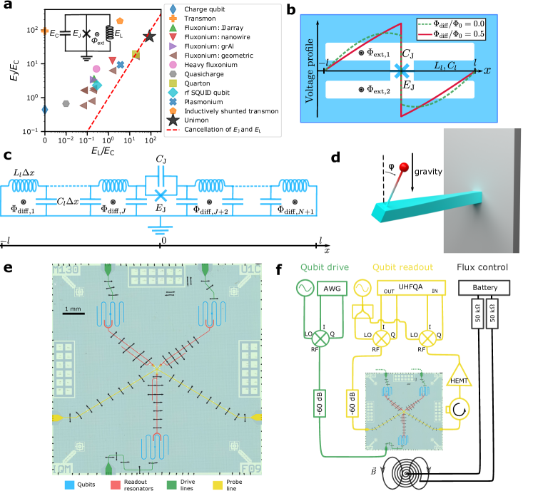
Figure 1: Unimon qubit and its measurement setup. Caption on the following page.

Figure 1: Unimon qubit and its measurement setup. a, Map of superconducting-qubit types based on their energy scales: Josephson energy $E_{\mathrm{J}}$ and inductive energy $E_{\textrm{L}}$ compared with the charging energy $E_{\mathrm{C}}$. The map includes those superconducting qubits that can be described with the circuit model shown in the inset. The proposed unimon qubit corresponds to the vicinity of the red dashed line leading to the cancellation of the linear inductive energy by the quadratic contribution of the Josephson energy at half flux quantum $\Phi_{0}/2$. The black star denotes the unimons realized in this work and the other experimental data points are from Refs.[73, 74, 75, 76, 42, 44, 41, 77, 78, 79, 46, 80]. b, Schematic illustration of the unimon circuit consisting of a Josephson junction ($E_{\mathrm{J}}$, $C_{\mathrm{J}}$) in a grounded coplanar-waveguide (CPW) resonator that has a length of $2l$ and an inductance and capacitance per unit length of $L_{l}$ and $C_{l}$, respectively. The voltage envelope functions of the qubit mode are also illustrated at external-flux biases $\Phi_{\mathrm{diff}}=(\Phi_{\mathrm{ext,2}}-\Phi_{\mathrm{ext,1}})/2=0.0$ (dashed line) and $\Phi_{\mathrm{diff}}=\Phi_{0}/2$ (solid line). c, Distributed-element circuit model of the unimon qubit, in which the CPW is modeled with $N$ inductors $L_{l}\Delta x$ and capacitors $C_{l}\Delta x$ with $\Delta x=2l/N$ denoting the length scale of discretization. d, Schematic illustration of a mechanical inverted pendulum system, the Hamiltonian of which is identical to that of the lumped-element unimon circuit in a. In this analogy, the gravitational potential energy corresponds to the Josephson potential, the harmonic potential energy of the twisting beam corresponds to the inductive energy, the moment of inertial corresponds to the capacitance of the unimon, and the angle of the zero twist position corresponds to the flux bias $\Phi_{\mathrm{diff}}$. e, False-color microscope image of a silicon chip containing three unimon qubits (blue) together with their readout resonators (red), drive lines (green), and a joint probe line (yellow). f, Simplified schematic of the experimental setup used to measure the unimon qubits at 10 mK (see also Extended Data Fig. 2).

Figure 2: Resonator and qubit B spectroscopies. a, Magnitude of the readout signal voltage transmitted through the probe line as a function of the signal frequency and the flux bias $\Phi_{\mathrm{diff}}$ of the unimon. b, Magnification at an avoided crossings of a, where a unimon and its readout resonator are close to resonance, together with a fit (solid black line) used to estimate the coupling capacitance $C_{\mathrm{g}}$ between the qubit and the resonator. The fit is based on diagonalizing equation (5) in Methods. c, Magnitude of the readout signal at a properly chosen readout frequency as a function of the flux bias $\Phi_{\mathrm{diff}}$ and qubit excitation frequency, revealing the spectral lines of the unimon together with global fits to the theoretical model 1 and 2 (Methods). The insets show magnifications at the flux sweet spots, highlighting that at half flux quantum, the unimon frequency is minimized whereas its anharmonicity is maximized.

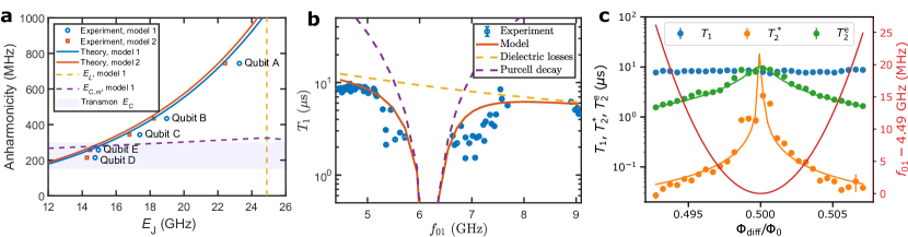
Figure 3: Measurement of key qubit properties. a, Measured anharmonicities of five unimon qubits (markers) at flux bias $\Phi_{\mathrm{diff}}=\Phi_{0}/2$ as functions of the Josephson energy $E_{\mathrm{J}}$ estimated from fits to the qubit spectroscopy data similar to Fig. 2c using the models 1 (blue color) and 2 (orange color) presented in Methods. The solid blue and orange lines show theoretical predictions of the anharmonicity based on models 1 and 2, respectively. The dashed yellow line illustrates the value of the Josephson energy $E_{\mathrm{J}}$ that perfectly cancels the linear inductive energy according to model 1. The capacitive energy $E_{C,m}$ of the qubit mode based on model 1 is shown with a dashed purple line, whereas the purple shading visualizes the typical anharmonicity of transmon qubits. b, Experimentally measured mean energy relaxation time $T_{1}$ of qubit B (blue circles) as a function of the qubit frequency $f_{01}$ together with a model (solid line) taking into account dielectric losses (dashed yellow line) and the Purcell decay (dashed purple line). The error bars represent the $1\sigma$ uncertainty obtained from 6–30 repetitions of single $T_{1}$ measurements conducted at each frequency. c, Relaxation time $T_{1}$, Ramsey coherence time $T_{2}^{*}$, and echo coherence time $T_{2}^{\mathrm{e}}$ of qubit B as functions of the flux bias $\Phi_{\mathrm{diff}}$ in the vicinity of the $\Phi_{0}/2$ flux sweet spot. The error bars represent the $1\sigma$ uncertainty based on 8 repeated experiments. The solid green and orange lines illustrate fits to $T_{2}^{\mathrm{e}}$ and $T_{2}^{*}$ data based on models regarding the dephasing rate as a linear function of $\partial f_{01}/\partial\Phi_{\mathrm{diff}}$ (Methods and Supplementary Note III). The solid red line shows the detuning of the qubit frequency from the minimum value of 4.49 GHz.

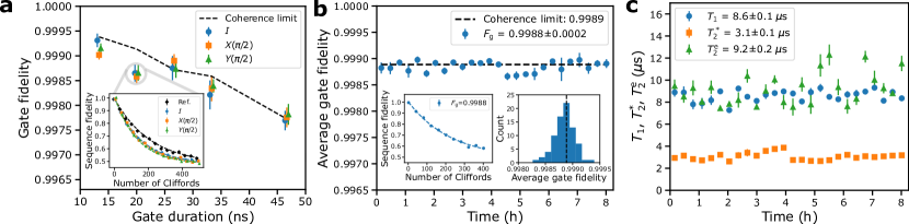
Figure 4: Implementation of fast and stable single-qubit gates for qubit B. a, Average gate fidelity as a function of the gate duration for gates in the set $\{I,X(\pi/2),Y(\pi/2)\}$. The error bars represent the $1\sigma$ uncertainty based on six interleaved randomized benchmarking experiments. The dashed black line shows the coherence limit computed based on the mean values of the energy relaxation time $T_{1}$ and the echo coherence time $T_{2}^{\mathrm{e}}$. The inset shows the results of an exemplary interleaved randomized benchmarking experiment corresponding to a gate duration of 20 ns. b, Average gate fidelity measured with randomized benchmarking as a function of time lapsed from the initial gate and parameter calibration. The error bars represent the $1\sigma$ uncertainty from three consecutive randomized benchmarking experiments. The dashed black line shows the coherence limit that has been computed using the mean values of $T_{1}$ and $T_{2}^{\mathrm{e}}$ measured interleaved with the gate fidelity. The left inset illustrates the decay of the sequence fidelity as a function of its length in an exemplary randomized-benchmarking experiment. The right inset shows the histogram of the gate fidelities obtained over the measurement period of eight hours. c, Stability of $T_{1}$, $T_{2}^{\mathrm{e}}$, and the Ramsey coherence time $T_{2}^{*}$ over a period of eight hours. The qubit parameters were calibrated only once before the characterization measurements. The error bars represent the $1\sigma$ uncertainty from three consecutive measurements.

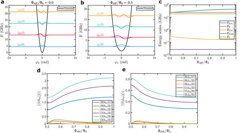
Extended Data Fig. 1: Potential-energy function, energy scales, and matrix elements of of qubit B based on model 1. a, b, Potential energy of the unimon based on equation (4) in Methods as a function of the phase variable $\varphi_{m}$ of mode $m$ together with the four lowest eigenenergies and corresponding phase-basis wave functions at flux biases of $\Phi_{\mathrm{diff}}=0$ (a) and $\Phi_{\mathrm{diff}}=\Phi_{0}/2$ (b). Note that the second mode of the circuit is used as the qubit at $\Phi_{\mathrm{diff}}=0$ and the first mode at $\Phi_{\mathrm{diff}}=\Phi_{0}/2$. c, Energy scales $E_{C,m}$, $E_{L,m}$, $E_{L}$, and $E_{\mathrm{J}}$ of the qubit as functions of $\Phi_{\mathrm{diff}}$. Here, $E_{C,m}$ and $E_{L,m}$ are the capacitive and inductive energies of the qubit mode, $E_{L}$ is the inductive energy corresponding to a dc current in the center conductor of the qubit, and $E_{\mathrm{J}}$ is the Josephson energy. We also show an effective charging energy $E_{C,\mathrm{tot}}=e^{2}/(4C_{l}l)$ computed based on the total capacitance $2C_{l}l$ of the transmission line of the unimon. d, Off-diagonal matrix elements of the Cooper pair number operator $\hat{n}_{m}$ for the four lowest-energy states of the qubit mode $m$ as functions of $\Phi_{\mathrm{diff}}$. e, As d but for the phase operator $\hat{\varphi}_{m}$. In all panels, the results have been obtained by using the theoretical model 1 in Methods and the measured parameter values of qubit B reported in Extended Data Table 1.

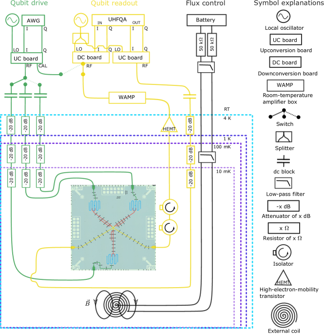
Extended Data Fig. 2: Experimental setup. Schematic experimental setup used in the measurements of the unimon qubits of this work. Electronics and components related to qubit drive, qubit readout, and flux control are denoted with green, yellow, and black colors, respectively. The dashed rectangles illustrate boundaries between the different temperature stages of the cryostat. Brief explanations of the symbols are provided in the rightmost column of the figure. Note that the qubit readout does not utilize any parametric amplifier.

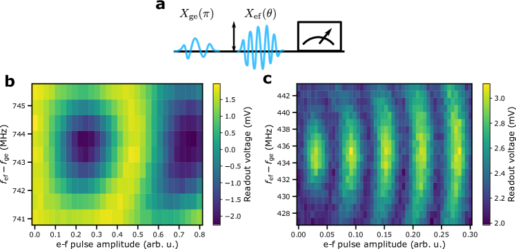
Extended Data Fig. 3: Estimation of qubit anharmonicity using Rabi oscillations. a Measurement sequence of an ef-Rabi experiment. In the experiment, the qubit is first prepared in the excited state with a $\pi$-pulse at the frequency $f_{\mathrm{ge}}$ matching with the qubit frequency $f_{01}$ followed by another pulse with a fixed duration but a varying frequency $f_{\mathrm{ef}}$ and a varying amplitude. After applying the pulses, the output readout voltage is measured. b,c Output readout voltage as a function of the amplitude of the ef-pulse and the frequency difference $f_{\mathrm{ef}}-f_{\mathrm{ge}}$ in an ef-Rabi experiment conducted for qubits A (b) and B (c). The resulting observed Rabi oscillations between the first and the second excited states of the unimon comfirm that the anharmonicities $\alpha$ of qubits A and B are approximately $2\pi\times 744$ MHz and $2\pi\times 434$ MHz, respectively, as measured using a two-tone qubit spectroscopy such as that shown in Fig. 2c.

Extended Data Fig. 4: Dispersive shift and single-shot qubit readout a, Measured dispersive shift $\chi$ for different unimon qubits at a flux bias of $\Phi_{\mathrm{diff}}=\Phi_{0}/2$ (blue circles) together with theoretical predictions (orange squares) computed using equation (8) in Methods based on the measured qubit frequency, measured anharmonicity, and the fitted coupling capacitance $C_{\mathrm{g}}$, all of which are reported in Extended Data Table 1. b, Readout voltages in the $IQ$ plane for a single-shot readout experiment conducted for qubit E. The qubit is prepared either to the ground state (blue dots) or to the excited state (orange dots) followed by a single-shot state measurement implemented using a readout pulse with a duration of 1.6 $\mu$s. The state preparation was repeated 2000 times for both the ground state and the excited state. The solid black line illustrates the optimal single-shot classification boundary corresponding to a readout fidelity of 89.0%. The classification errors are 5.0% and 17.0% when preparing the qubit to the ground state and to the excited state, respectively. c, Probability density distributions for the single-shot voltage corresponding to the qubit prepared to the ground state (blue dots) or to the excited state (orange dots). The single-shot voltages have been projected along a line perpendicular to the classification boundary. The solid lines denote fits to the measured probability densities based on a model involving a sum of two Gaussian functions.

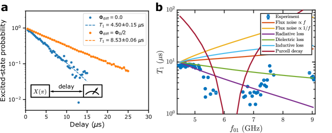
Extended Data Fig. 5: Characterization of the energy relaxation time for qubit B. a, Excited-state probability as a function of the length of the delay between the state preparation and readout (see inset) at the sweet spots $\Phi_{\mathrm{diff}}=0$ (blue color) and $\Phi_{\mathrm{diff}}=\Phi_{0}/2$ (orange color). The slopes of the exponential fits (dashed lines) yield energy relaxation times $T_{1}=4.5\pm 0.2$ $\mu$s and $T_{1}=8.5\pm 0.1$ $\mu$s at $\Phi_{\mathrm{diff}}=0$ and $\Phi_{0}/2$, respectively. b, Measured mean $T_{1}$ as a function of the qubit frequency (blue circles) together with theoretical predictions of $T_{1}$ based on different indicated loss mechanisms including Ohmic flux noise, $1/f$ flux noise, radiative losses, dielectric losses, inductive losses, and Purcell decay through the resonator. The error bars provide the $1\sigma$ uncertainty. The theoretical predictions (apart from the Purcell decay) have been scaled to coincide with the experimental data at $\Phi_{\mathrm{diff}}=\Phi_{0}/2$.

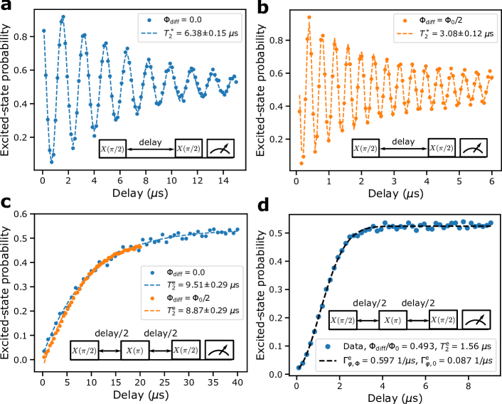
Extended Data Fig. 6: Characterization of the coherence time for qubit B. a, Excited-state probability as a function of the length of the delay between the $X(\pi/2)$ pulses of a Ramsey measurement (see inset) conducted at the sweet spot $\Phi_{\mathrm{diff}}=0$ using a detuning of 0.6 MHz between the drive frequency and the qubit frequency. The markers show the experimental data and the dash line provides a corresponding least-squares fit of an exponentially decaying sinusoidal function. b, As a but for $\Phi_{\mathrm{diff}}=\Phi_{0}/2$ and a detuning of 2.5 MHz between the drive frequency and the qubit frequency. c, Measured excited-state probability (markers) as a function of the length of the delay between the $X(\pi/2)$ pulses in a $T_{2}$ echo measurement (see inset) conducted at the sweet spots $\Phi_{\mathrm{diff}}=0$ (blue color) and $\Phi_{\mathrm{diff}}=\Phi_{0}/2$ (orange color). The dash lines provide exponential fits to the data. d Same as c but for a flux bias of $\Phi_{\mathrm{diff}}/\Phi_{0}=0.493$. Here, the dashed line shows a model corresponding to a product of a Gaussian and an exponential with decay rates $\Gamma_{\varphi,\Phi}^{\mathrm{e}}=0.60$ 1/$\mu$s and $\Gamma_{\varphi,0}^{\mathrm{e}}=0.09$ 1/$\mu$s, respectively.

Extended Data Table 1: Characteristic parameter values for the five measured unimon qubits. For each of the characterized qubits, the data includes the total length $2l$ of the center conductor in the qubit, the fitted inductance $L_{l}$ and capacitance $C_{l}$ per unit length of the center conductor, the fitted Josephson energy $E_{\mathrm{J}}$, the inductive and capacitive energies $E_{L,m}$ and $E_{C,m}$, the measured qubit frequency $\omega_{01}/(2\pi)$, the measured anharmonicity $\alpha/(2\pi)$, the location $x_{\mathrm{g}}$ of the unimon–resonator coupling point with respect to the junction, the measured coupling strength $|g_{01}|/(2\pi)$ between the qubit and its readout resonator providing the corresponding coupling capacitance $C_{\mathrm{g}}$, the measured dispersive shift $\chi/(2\pi)$, the measured frequency of the readout resonator $f_{\mathrm{r}}$, and the measured linewidth of the readout resonator $\kappa/(2\pi)$. All the fitted values were estimated using theory model 1 (Methods). The values of the flux-dependent quantities $E_{L,m}$, $E_{C,m}$, $\omega_{01}/(2\pi)$, $\alpha/(2\pi)$, $g_{01}/(2\pi)$, $\chi/(2\pi)$, and $f_{\mathrm{r}}$ are reported at $\Phi_{\mathrm{diff}}=\Phi_{0}/2$. The asterisks denote the fact that the inductance $L_{l}$ and capacitance $C_{l}$ per unit length are estimated by fitting the theoretical model to the spectrum of qubit B and that equal values are used for the other qubits due to an identical cross section of the co-planar waveguide in all qubits. The inductive and capacitive energies $E_{L,m}$ and $E_{C,m}$ are computed using the theoretical model 1 (Methods) which is also used to obtain the measured values of $E_{\mathrm{J}}$, $L_{l}$ and $C_{l}$.

Qubit	$2l$	$L_{l}$	$C_{l}$	$E_{\mathrm{J}}/h$	$E_{L,m}/h$	$E_{C,m}/h$	$\omega_{01}/(2\pi)$	$\alpha/(2\pi)$	$x_{\mathrm{g}}$	$C_{\mathrm{g}}$	$|g_{01}|/(2\pi)$	$\chi/(2\pi)$	$f_{r}$	$\kappa/(2\pi)$
	(mm)	($\mu$H/m)	(pF/m)	(GHz)	(GHz)	(GHz)	(GHz)	(MHz)	(mm)	(fF)	(MHz)	(MHz)	(GHz)	(MHz)
A	8.0	0.821∗	87.1∗	23.3	24.9	0.318	3.547	744	0.596	9	53.5	0.74	5.826	0.43
B	8.0	0.821	87.1	19.0	25.2	0.297	4.488	434	0.596	10	70.0	1.2	6.198	1.24
C	8.0	0.821∗	87.1∗	17.4	25.3	0.290	4.781	343	0.596	12.5	79.7	9.20	5.522	9.2
D	8.0	0.821∗	87.1∗	14.8	25.7	0.278	5.257	214	0.596	12.5	85.7	20.2	5.699	10.0
E	8.0	0.821∗	87.1∗	15.0	25.7	0.279	5.224	257	0.596	12.5	92.3	4.1	6.156	1.8

Extended Data Table 2: Results of coherence characterization and randomized-benchmarking (RB) experiments for the five unimon qubits. The measured energy relaxation time $T_{1}$, the measured Ramsey coherence time $T_{2}^{*}$, the measured echo coherence time $T_{2}^{\mathrm{e}}$, the flux noise density parameter $A_{\Phi_{\mathrm{diff}}}$ at 1 Hz estimated from the echo coherence time, the average fidelity per microwave gate from standard RB experiments, and the gate duration used in the RB experiments. All of the values are measured in the immediate vicinity of the sweet spot $\Phi_{\mathrm{diff}}=\Phi_{0}/2$.

	$\Phi_{\mathrm{diff}}=\Phi_{0}/2$
Qubit	$T_{1}$	$T_{2}^{*}$	$T_{2}^{\mathrm{e}}$	$A_{\Phi_{\mathrm{diff}}}$	RB fidelity	Gate duration
	($\mu$s)	($\mu$s)	($\mu$s)	($\mu\Phi_{0}$)	(%)	(ns)
A	7.2	1.9	6.8	6.1	99.81	13.3
B	8.6	3.1	9.2	15.0	99.90	13.3
C	5.8	2.3	9.3	11.2	99.54	40
D	3.9	2.3	7.0	11.1	99.63	20
E	5.6	2.5	11.4	14.3	99.86	13.3

Extended Data Table 3: Design values of the characteristic parameters of the five unimon qubits. The design values listed in the table include the inductance $L_{l}$ and capacitance $C_{l}$ per unit length of the center conductor of the qubit, the characteristic impedance $Z$ of the transmission line in the qubit, the coupling capacitance $C_{\mathrm{g}}$ and coupling strength $|g_{01}|/(2\pi)$ between the qubit and its readout resonator, the coupling capacitance $C_{\mathrm{d}}$ between the qubit and its drive line, the dispersive shift $\chi/(2\pi)$ of the qubit, the frequency $f_{r}$ of the readout resonator, the coupling capacitance $C_{\kappa}$ between the readout resonator and the readout transmission line, and the linewidth of the readout resonator $\kappa/(2\pi)$. Note that the coupling strength $|g_{01}|/(2\pi)$ is estimated by a simulation, in which the resonator frequency is tuned on resonance with a linearized unimon circuit in order to measure $|g_{01}|/(2\pi)$ from the frequency separation of the resonances in the formed avoided crossing.

Qubit	$L_{l}$	$C_{l}$	$Z$	$C_{\mathrm{g}}$	$|g_{01}|/(2\pi)$	$C_{\mathrm{d}}$	$\chi/(2\pi)$	$f_{r}$	$C_{\kappa}$	$\kappa/(2\pi)$
	($\mu$H/m)	(pF/m)	($\Omega$)	(fF)	(MHz)	(fF)	(MHz)	(GHz)	(fF)	(MHz)
A	0.83	83	100	10.4	53.2	0.083	0.89	6.0	16.8	0.89
B	0.83	83	100	10.4	53.2	0.083	0.58	6.3	12.8	0.58
C	0.83	83	100	14.0	69.4	0.083	2.48	5.7	29.6	2.48
D	0.83	83	100	14.0	69.4	0.083	1.44	6.0	28.1	1.44
E	0.83	83	100	14.0	69.4	0.083	0.94	6.3	21.5	0.94

References

- [1] Krantz, P. et al. A quantum engineer’s guide to superconducting qubits. Applied Physics Reviews 6, 021318 (2019).
- [2] Blais, A., Grimsmo, A. L., Girvin, S. & Wallraff, A. Circuit quantum electrodynamics. Reviews of Modern Physics 93, 025005 (2021). URL https://link.aps.org/doi/10.1103/RevModPhys.93.025005. Publisher: American Physical Society.
- [3] Yanay, Y., Braumüller, J., Gustavsson, S., Oliver, W. D. & Tahan, C. Two-dimensional hard-core bose–hubbard model with superconducting qubits. npj Quantum Information 6, 1–12 (2020).
- [4] Farhi, E., Goldstone, J. & Gutmann, S. A Quantum Approximate Optimization Algorithm. arXiv:1411.4028 [quant-ph] (2014). URL http://arxiv.org/abs/1411.4028. ArXiv: 1411.4028.
- [5] Dunjko, V. & Briegel, H. J. Machine learning & artificial intelligence in the quantum domain: a review of recent progress. Reports on Progress in Physics 81, 074001 (2018). URL https://doi.org/10.1088/1361-6633/aab406. Publisher: IOP Publishing.
- [6] McArdle, S., Endo, S., Aspuru-Guzik, A., Benjamin, S. C. & Yuan, X. Quantum computational chemistry. Reviews of Modern Physics 92, 015003 (2020). URL https://link.aps.org/doi/10.1103/RevModPhys.92.015003.
- [7] Arute, F. et al. Quantum supremacy using a programmable superconducting processor. Nature 574, 505–510 (2019). URL https://www.nature.com/articles/s41586-019-1666-5.
- [8] Wu, Y. et al. Strong quantum computational advantage using a superconducting quantum processor. arXiv:2106.14734 [quant-ph] (2021). URL http://arxiv.org/abs/2106.14734. ArXiv: 2106.14734.
- [9] Ofek, N. et al. Extending the lifetime of a quantum bit with error correction in superconducting circuits. Nature 536 (2016). URL https://www.nature.com/articles/nature18949.
- [10] Campagne-Ibarcq, P. et al. Quantum error correction of a qubit encoded in grid states of an oscillator. Nature 584 (2020). URL https://www.nature.com/articles/s41586-020-2603-3.
- [11] Chen, Z. et al. Exponential suppression of bit or phase errors with cyclic error correction. Nature 595 (2021). URL https://www.nature.com/articles/s41586-021-03588-y.
- [12] Koch, J. et al. Charge-insensitive qubit design derived from the Cooper pair box. Physical Review A 76, 042319 (2007). URL https://link.aps.org/doi/10.1103/PhysRevA.76.042319.
- [13] Nguyen, L. B. et al. High-Coherence Fluxonium Qubit. Physical Review X 9, 041041 (2019). URL https://link.aps.org/doi/10.1103/PhysRevX.9.041041. Publisher: American Physical Society.
- [14] Pechenezhskiy, I. V., Mencia, R. A., Nguyen, L. B., Lin, Y.-H. & Manucharyan, V. E. The superconducting quasicharge qubit. Nature 585, 368–371 (2020). URL https://www.nature.com/articles/s41586-020-2687-9. Bandiera_abtest: a Cg_type: Nature Research Journals Number: 7825 Primary_atype: Research Publisher: Nature Publishing Group Subject_term: Quantum information;Qubits;Superconducting devices Subject_term_id: quantum-information;qubits;superconducting-devices.
- [15] Gyenis, A. et al. Experimental Realization of a Protected Superconducting Circuit Derived from the $0$–$\ensuremath{\pi}$ Qubit. PRX Quantum 2, 010339 (2021). URL https://link.aps.org/doi/10.1103/PRXQuantum.2.010339.
- [16] Yan, F. et al. Engineering Framework for Optimizing Superconducting Qubit Designs. arXiv:2006.04130 [quant-ph] (2020). URL http://arxiv.org/abs/2006.04130. ArXiv: 2006.04130.
- [17] Preskill, J. Quantum Computing in the NISQ era and beyond. Quantum 2, 79 (2018). URL https://quantum-journal.org/papers/q-2018-08-06-79/.
- [18] Nakahara, M. Quantum computing: from linear algebra to physical realizations (CRC press, 2008).
- [19] Temme, K., Bravyi, S. & Gambetta, J. M. Error mitigation for short-depth quantum circuits. Physical review letters 119, 180509 (2017).
- [20] Kandala, A. et al. Error mitigation extends the computational reach of a noisy quantum processor. Nature 567, 491–495 (2019).
- [21] Gottesman, D. Stabilizer codes and quantum error correction. Ph.D. thesis, California Institute of Technology (1997).
- [22] Fowler, A. G., Mariantoni, M., Martinis, J. M. & Cleland, A. N. Surface codes: Towards practical large-scale quantum computation. Physical Review A 86, 032324 (2012). URL https://link.aps.org/doi/10.1103/PhysRevA.86.032324.
- [23] Bonilla Ataides, J. P., Tuckett, D. K., Bartlett, S. D., Flammia, S. T. & Brown, B. J. The xzzx surface code. Nature communications 12, 1–12 (2021).
- [24] Barends, R. et al. Superconducting quantum circuits at the surface code threshold for fault tolerance. Nature 508, 500–503 (2014). URL https://www.nature.com/articles/nature13171.
- [25] Andersen, C. K. et al. Repeated quantum error detection in a surface code. Nature Physics 16, 875–880 (2020). URL https://www.nature.com/articles/s41567-020-0920-y.
- [26] Marques, J. et al. Logical-qubit operations in an error-detecting surface code. Nature Physics 1–7 (2021).
- [27] Krinner, S. et al. Realizing repeated quantum error correction in a distance-three surface code. arXiv preprint arXiv:2112.03708 (2021).
- [28] Zhao, Y. et al. Realizing an error-correcting surface code with superconducting qubits. arXiv preprint arXiv:2112.13505 (2021).
- [29] Hertzberg, J. B. et al. Laser-annealing josephson junctions for yielding scaled-up superconducting quantum processors. npj Quantum Information 7, 1–8 (2021).
- [30] Zhu, Q. et al. Quantum computational advantage via 60-qubit 24-cycle random circuit sampling. Science Bulletin (2021).
- [31] Place, A. P. M. et al. New material platform for superconducting transmon qubits with coherence times exceeding 0.3 milliseconds. Nature Communications 12, 1779 (2021). URL https://www.nature.com/articles/s41467-021-22030-5.
- [32] Wang, C. et al. Towards practical quantum computers: transmon qubit with a lifetime approaching 0.5 milliseconds. npj Quantum Information 8, 1–6 (2022).
- [33] McKay, D. C., Wood, C. J., Sheldon, S., Chow, J. M. & Gambetta, J. M. Efficient z gates for quantum computing. Physical Review A 96, 022330 (2017).
- [34] Sung, Y. et al. Realization of High-Fidelity CZ and ZZ-Free iSWAP Gates with a Tunable Coupler. Physical Review X 11, 021058 (2021). URL https://link.aps.org/doi/10.1103/PhysRevX.11.021058. Publisher: American Physical Society.
- [35] Nakamura, Y., Pashkin, Y. A. & Tsai, J. S. Coherent control of macroscopic quantum states in a single-Cooper-pair box. Nature 398, 786–788 (1999). URL https://www.nature.com/articles/19718.
- [36] Barends, R. et al. Coherent Josephson Qubit Suitable for Scalable Quantum Integrated Circuits. Physical Review Letters 111, 080502 (2013). URL https://link.aps.org/doi/10.1103/PhysRevLett.111.080502.
- [37] Wood, C. J. & Gambetta, J. M. Quantification and characterization of leakage errors. Physical Review A 97, 032306 (2018).
- [38] Lescanne, R. et al. Escape of a Driven Quantum Josephson Circuit into Unconfined States. Physical Review Applied 11, 014030 (2019). URL https://link.aps.org/doi/10.1103/PhysRevApplied.11.014030. Publisher: American Physical Society.
- [39] Manucharyan, V. E., Koch, J., Glazman, L. I. & Devoret, M. H. Fluxonium: Single Cooper-Pair Circuit Free of Charge Offsets. Science 326, 113–116 (2009). URL https://science.sciencemag.org/content/326/5949/113.
- [40] Bao, F. et al. Fluxonium: an alternative qubit platform for high-fidelity operations. arXiv preprint arXiv:2111.13504 (2021).
- [41] Zhang, H. et al. Universal fast-flux control of a coherent, low-frequency qubit. Physical Review X 11, 011010 (2021).
- [42] Grünhaupt, L. et al. Granular aluminium as a superconducting material for high-impedance quantum circuits. Nature materials 18, 816–819 (2019).
- [43] Hazard, T. et al. Nanowire Superinductance Fluxonium Qubit. Physical Review Letters 122, 010504 (2019). URL https://link.aps.org/doi/10.1103/PhysRevLett.122.010504. Publisher: American Physical Society.
- [44] Peruzzo, M. et al. Geometric superinductance qubits: Controlling phase delocalization across a single josephson junction. PRX Quantum 2, 040341 (2021). URL https://link.aps.org/doi/10.1103/PRXQuantum.2.040341.
- [45] Earnest, N. et al. Realization of a Lambda-System with Metastable States of a Capacitively Shunted Fluxonium. Physical Review Letters 120, 150504 (2018). URL https://link.aps.org/doi/10.1103/PhysRevLett.120.150504.
- [46] Liu, F.-M. et al. Quantum design for advanced qubits. arXiv preprint arXiv:2109.00994 (2021).
- [47] Kalashnikov, K. et al. Bifluxon: Fluxon-parity-protected superconducting qubit. PRX Quantum 1, 010307 (2020).
- [48] Smith, W., Kou, A., Xiao, X., Vool, U. & Devoret, M. Superconducting circuit protected by two-cooper-pair tunneling. npj Quantum Information 6, 1–9 (2020).
- [49] Blais, A., Huang, R.-S., Wallraff, A., Girvin, S. M. & Schoelkopf, R. J. Cavity quantum electrodynamics for superconducting electrical circuits: An architecture for quantum computation. Physical Review A 69, 062320 (2004). URL https://link.aps.org/doi/10.1103/PhysRevA.69.062320.
- [50] Siddiqi, I. et al. Dispersive measurements of superconducting qubit coherence with a fast latching readout. Physical Review B 73, 054510 (2006).
- [51] Peruzzo, M., Trioni, A., Hassani, F., Zemlicka, M. & Fink, J. M. Surpassing the Resistance Quantum with a Geometric Superinductor. Physical Review Applied 14, 044055 (2020). URL https://link.aps.org/doi/10.1103/PhysRevApplied.14.044055. Publisher: American Physical Society.
- [52] Braumüller, J. et al. Characterizing and optimizing qubit coherence based on squid geometry. Physical Review Applied 13, 054079 (2020).
- [53] Motzoi, F., Gambetta, J. M., Rebentrost, P. & Wilhelm, F. K. Simple Pulses for Elimination of Leakage in Weakly Nonlinear Qubits. Physical Review Letters 103, 110501 (2009). URL https://link.aps.org/doi/10.1103/PhysRevLett.103.110501. Publisher: American Physical Society.
- [54] Chow, J. M. et al. Optimized driving of superconducting artificial atoms for improved single-qubit gates. Physical Review A 82, 040305 (2010). URL https://link.aps.org/doi/10.1103/PhysRevA.82.040305. Publisher: American Physical Society.
- [55] Magesan, E. et al. Efficient measurement of quantum gate error by interleaved randomized benchmarking. Physical review letters 109, 080505 (2012).
- [56] Magesan, E., Gambetta, J. M. & Emerson, J. Scalable and Robust Randomized Benchmarking of Quantum Processes. Physical Review Letters 106, 180504 (2011). URL https://link.aps.org/doi/10.1103/PhysRevLett.106.180504. Publisher: American Physical Society.
- [57] Magesan, E., Gambetta, J. M. & Emerson, J. Characterizing quantum gates via randomized benchmarking. Physical Review A 85, 042311 (2012). URL https://link.aps.org/doi/10.1103/PhysRevA.85.042311.
- [58] Lahtinen, V. & Möttönen, M. Effects of device geometry and material properties on dielectric losses in superconducting coplanar-waveguide resonators. Journal of Physics: Condensed Matter 32, 405702 (2020). URL https://doi.org/10.1088/1361-648x/ab98c8. Publisher: IOP Publishing.
- [59] Yan, F. et al. Tunable Coupling Scheme for Implementing High-Fidelity Two-Qubit Gates. Physical Review Applied 10, 054062 (2018). URL https://link.aps.org/doi/10.1103/PhysRevApplied.10.054062. Publisher: American Physical Society.
- [60] Zhao, P. et al. High-contrast z z interaction using superconducting qubits with opposite-sign anharmonicity. Physical Review Letters 125, 200503 (2020).
- [61] Bourassa, J., Beaudoin, F., Gambetta, J. M. & Blais, A. Josephson-junction-embedded transmission-line resonators: From kerr medium to in-line transmon. Physical Review A 86, 013814 (2012).
- [62] Vool, U. & Devoret, M. Introduction to quantum electromagnetic circuits. International Journal of Circuit Theory and Applications 45, 897–934 (2017).
- [63] Heinsoo, J. et al. KQCircuits (2021). URL https://github.com/iqm-finland/KQCircuits.
- [64] Köfferlein, M. KLayout (2021). URL https://www.klayout.de/.
- [65] Simons, R. N. Coplanar waveguide circuits, components, and systems (John Wiley & Sons, 2004).
- [66] Schoelkopf, R., Clerk, A., Girvin, S., Lehnert, K. & Devoret, M. Qubits as spectrometers of quantum noise. In Quantum noise in mesoscopic physics, 175–203 (Springer, 2003).
- [67] Bylander, J. et al. Noise spectroscopy through dynamical decoupling with a superconducting flux qubit. Nature Physics 7, 565–570 (2011).
- [68] Yan, F. et al. The flux qubit revisited to enhance coherence and reproducibility. Nature Communications 7, 12964 (2016). URL https://www.nature.com/articles/ncomms12964.
- [69] Ithier, G. et al. Decoherence in a superconducting quantum bit circuit. Physical Review B 72, 134519 (2005).
- [70] Reed, M. Entanglement and quantum error correction with superconducting qubits. Ph.D. thesis, Yale University (2013).
- [71] Nielsen, M. A. A simple formula for the average gate fidelity of a quantum dynamical operation. Physics Letters A 303, 249–252 (2002).
- [72] Epstein, J. M., Cross, A. W., Magesan, E. & Gambetta, J. M. Investigating the limits of randomized benchmarking protocols. Physical Review A 89, 062321 (2014). URL https://link.aps.org/doi/10.1103/PhysRevA.89.062321.
- [73] Nakamura, Y., Pashkin, Y. A. & Tsai, J. Coherent control of macroscopic quantum states in a single-cooper-pair box. nature 398, 786–788 (1999).
- [74] Barends, R. et al. Coherent josephson qubit suitable for scalable quantum integrated circuits. Physical review letters 111, 080502 (2013).
- [75] Manucharyan, V. E., Koch, J., Glazman, L. I. & Devoret, M. H. Fluxonium: Single cooper-pair circuit free of charge offsets. Science 326, 113–116 (2009).
- [76] Hazard, T. et al. Nanowire superinductance fluxonium qubit. Physical review letters 122, 010504 (2019).
- [77] Pechenezhskiy, I. V., Mencia, R. A., Nguyen, L. B., Lin, Y.-H. & Manucharyan, V. E. The superconducting quasicharge qubit. Nature 585, 368–371 (2020).
- [78] Yan, F. et al. Engineering framework for optimizing superconducting qubit designs. arXiv preprint arXiv:2006.04130 (2020).
- [79] Peltonen, J. et al. Hybrid rf squid qubit based on high kinetic inductance. Scientific reports 8, 1–8 (2018).
- [80] Hassani, F. et al. A superconducting qubit with noise-insensitive plasmon levels and decay-protected fluxon states. arXiv preprint arXiv:2202.13917 (2022).