Improved uniform error bounds on time-splitting methods for the long-time dynamics of the weakly nonlinear Dirac equation

Weizhu Bao
Department of Mathematics
Email: matbaowz@nus.edu.sg
National University of Singapore Singapore 119076 Singapore
Yongyong Cai
Laboratory of Mathematics and Complex Systems and School of Mathematical Sciences
Email: yongyong.cai@bnu.edu.cn
Beijing Normal University Beijing 100875 China
and
Yue Feng
Department of Mathematics
Email: fengyue@u.nus.edu
National University of Singapore Singapore 119076 Singapore
Abstract

Improved uniform error bounds on time-splitting methods are rigorously proven for the long-time dynamics of the weakly nonlinear Dirac equation (NLDE), where the nonlinearity strength is characterized by a dimensionless parameter ε(0,1]𝜀01\varepsilon\in(0,1] . We adopt a second order Strang splitting method to discretize the NLDE in time and combine the Fourier pseudospectral method in space for the full-discretization. By employing the regularity compensation oscillation (RCO) technique where the high frequency modes are controlled by the regularity of the exact solution and the low frequency modes are analyzed by phase cancellation and energy method, we establish improved uniform error bounds at O(ε2τ2)𝑂superscript𝜀2superscript𝜏2O(\varepsilon^{2}\tau^{2}) and O(hm1+ε2τ2)𝑂superscript𝑚1superscript𝜀2superscript𝜏2O(h^{m-1}+\varepsilon^{2}\tau^{2}) for the second-order Strang splitting semi-discretizaion and full-discretization up to the long-time Tε=T/ε2subscript𝑇𝜀𝑇superscript𝜀2T_{\varepsilon}=T/\varepsilon^{2} with T>0𝑇0T>0 fixed, respectively. Furthermore, the numerical scheme and error estimates are extended to an oscillatory NLDE which propagates waves with O(ε2)𝑂superscript𝜀2O(\varepsilon^{2}) wavelength in time and at O(ε2)𝑂superscript𝜀2O(\varepsilon^{-2}) wave speed in space. Finally, numerical examples verifying our analytical results are given. nonlinear Dirac equation; long-time dynamics; time-splitting method; improved uniform error bound; regularity compensation oscillation (RCO).

1 Introduction

Long-time dynamics of Hamiltonian partial differential equation (PDE) has attracted much interest in recent years from both analytical and numerical aspects (Cazenave & Vazquez, 1986; Faou & Greébert, 2011; Faou et al., 2011; Sasaki, 2015). The change of a small nonlinear perturbation to the dynamics of a linear Hamiltonian PDE deserves careful considerations (Gauckler & Lubich, 2010; Hairer & Lubich, 2009). The nonlinear Dirac equation (NLDE) is widely used in many fields such as the electron self-interaction (Dirac, 1928; Esteban & Séré, 1997), quantum field theory (Thirring, 1958; Soler, 1970), Bose-Einstein condensate (BEC) (Haddad & Carr, 2009) and graphene as well as other 2D materials (Brinkman et al., 2014; Fefferman & Weistein, 2012). In this paper, we study the dynamics of the weakly NLDE in one or two dimensions (1D or 2D), which can be expressed for the two-component wave function Φ:=Φ(t,𝐱)=(ϕ1(t,𝐱),ϕ2(t,𝐱))T2assignΦΦ𝑡𝐱superscriptsubscriptitalic-ϕ1𝑡𝐱subscriptitalic-ϕ2𝑡𝐱𝑇superscript2\Phi:=\Phi(t,{\bf x})=(\phi_{1}(t,{\bf x}),\phi_{2}(t,{\bf x}))^{T}\in{\mathbb{C}}^{2} as (Dirac, 1928, 1958)

itΦ=(ij=1dσjj+σ3)Φ+ε2𝐅(Φ)Φ,xΩ,t>0,formulae-sequence𝑖subscript𝑡Φ𝑖superscriptsubscript𝑗1𝑑subscript𝜎𝑗subscript𝑗subscript𝜎3Φsuperscript𝜀2𝐅ΦΦformulae-sequence𝑥Ω𝑡0i\partial_{t}\Phi=\Big{(}-i\sum_{j=1}^{d}\sigma_{j}\partial_{j}+\sigma_{3}\Big{)}\Phi+\varepsilon^{2}{{\bf F}}(\Phi)\Phi,\quad x\in\Omega,\quad t>0, (1.0.1)

with the initial data

Φ(t=0,𝐱)=Φ0(𝐱),𝐱Ω¯,formulae-sequenceΦ𝑡0𝐱subscriptΦ0𝐱𝐱¯Ω\Phi(t=0,{\bf x})=\Phi_{0}({\bf x}),\quad{\bf x}\in\overline{\Omega}, (1.0.2)

where Ω=j=1d(aj,bj)dΩsubscriptsuperscriptproduct𝑑𝑗1subscript𝑎𝑗subscript𝑏𝑗superscript𝑑\Omega=\prod^{d}_{j=1}(a_{j},b_{j})\subset\mathbb{R}^{d} (d=1,2𝑑12d=1,2) is a bounded domain equipped with periodic boundary conditions. Here, i=1𝑖1i=\sqrt{-1} is the imaginary unit, t𝑡t is time, 𝐱=(x1,,xd)T𝐱superscriptsubscript𝑥1subscript𝑥𝑑𝑇\mathbf{x}=(x_{1},\ldots,x_{d})^{T} is the spatial coordinate vector, jsubscript𝑗\partial_{j} represents xjsubscriptsubscript𝑥𝑗\partial_{x_{j}} for j=1,,d𝑗1𝑑j=1,\ldots,d, ε(0,1]𝜀01\varepsilon\in(0,1] is a dimensionless parameter. σ1subscript𝜎1\sigma_{1}, σ2subscript𝜎2\sigma_{2} and σ3subscript𝜎3\sigma_{3} are the Pauli matrices given as

σ1=(0 11 0),σ2=(0ii 0),σ3=(1 001).formulae-sequencesubscript𝜎1matrix011 0formulae-sequencesubscript𝜎2matrix0𝑖𝑖 0subscript𝜎3matrix1 001\sigma_{1}=\begin{pmatrix}0&\ 1\\ 1&\ 0\end{pmatrix},\quad\sigma_{2}=\begin{pmatrix}0&\ -i\\ i&\ 0\end{pmatrix},\quad\sigma_{3}=\begin{pmatrix}1&\ 0\\ 0&\ -1\end{pmatrix}. (1.0.3)

The matrix nonlinearity 𝐅(Φ)𝐅Φ{\bf F}(\Phi) in (1.0.1) is usually taken as

𝐅(Φ)=λ1(Φσ3Φ)σ3+λ2|Φ|2I2,Φ2,formulae-sequence𝐅Φsubscript𝜆1superscriptΦsubscript𝜎3Φsubscript𝜎3subscript𝜆2superscriptΦ2subscript𝐼2Φsuperscript2{{\bf F}}(\Phi)=\lambda_{1}(\Phi^{\ast}\sigma_{3}\Phi)\sigma_{3}+\lambda_{2}|\Phi|^{2}I_{2},\quad\Phi\in\mathbb{C}^{2}, (1.0.4)

where λ1subscript𝜆1\lambda_{1}, λ2subscript𝜆2\lambda_{2} are two given real constants, I2subscript𝐼2I_{2} is the 2×2222\times 2 identity matrix and |Φ|2=ΦΦsuperscriptΦ2superscriptΦΦ|\Phi|^{2}=\Phi^{\ast}\Phi with Φ=Φ¯TsuperscriptΦsuperscript¯Φ𝑇\Phi^{\ast}=\bar{\Phi}^{T} representing the complex conjugate transpose of ΦΦ\Phi. The choice of the nonlinearity 𝐅(Φ)𝐅Φ{\bf F}(\Phi) is motivated by the so-called Soler model in quantum field theory, e.g., λ10subscript𝜆10\lambda_{1}\neq 0 and λ2=0subscript𝜆20\lambda_{2}=0 (Fushchich & Shtelen, 1983; Thirring, 1958; Soler, 1970), and the BEC with a chiral confinement and/or spin-orbit coupling, e.g., λ1=0subscript𝜆10\lambda_{1}=0 and λ20subscript𝜆20\lambda_{2}\neq 0 (Chang et al., 1975; Haddad & Carr, 2009).

The NLDE (1.0.1) is dispersive and time symmetric (Bao et al., 2016). In addition, it conserves the total mass as

Φ(t,)2:=Ω|Φ(t,𝐱)|2𝑑𝐱=Ωj=12|ϕj(t,𝐱)|2d𝐱Φ(0,)2=Φ02,t0,formulae-sequenceassignsuperscriptnormΦ𝑡2subscriptΩsuperscriptΦ𝑡𝐱2differential-d𝐱subscriptΩsubscriptsuperscript2𝑗1superscriptsubscriptitalic-ϕ𝑗𝑡𝐱2𝑑𝐱superscriptnormΦ02superscriptnormsubscriptΦ02𝑡0\left\|\Phi(t,\cdot)\right\|^{2}:=\int_{\Omega}|\Phi(t,{\bf x})|^{2}d{\bf x}=\int_{\Omega}\sum^{2}_{j=1}|\phi_{j}(t,{\bf x})|^{2}d{\bf x}\equiv\left\|\Phi(0,\cdot)\right\|^{2}=\left\|\Phi_{0}\right\|^{2},\quad t\geq 0, (1.0.5)

and the energy as

E(t):=Ω(ij=1dΦσjjΦ+Φσ3Φ+ε2G(Φ))𝑑𝐱E(0),t0,formulae-sequenceassign𝐸𝑡subscriptΩ𝑖superscriptsubscript𝑗1𝑑superscriptΦsubscript𝜎𝑗subscript𝑗ΦsuperscriptΦsubscript𝜎3Φsuperscript𝜀2𝐺Φdifferential-d𝐱𝐸0𝑡0E(t):=\int_{\Omega}\Big{(}-i\sum_{j=1}^{d}\Phi^{*}\sigma_{j}\partial_{j}\Phi+\Phi^{*}\sigma_{3}\Phi+\varepsilon^{2}G(\Phi)\Big{)}d{\bf x}\equiv E(0),\quad t\geq 0, (1.0.6)

where

G(Φ)=λ12(Φσ3Φ)2+λ22|Φ|4,Φ2.formulae-sequence𝐺Φsubscript𝜆12superscriptsuperscriptΦsubscript𝜎3Φ2subscript𝜆22superscriptΦ4Φsuperscript2G(\Phi)=\frac{\lambda_{1}}{2}\left(\Phi^{*}\sigma_{3}\Phi\right)^{2}+\frac{\lambda_{2}}{2}|\Phi|^{4},\quad\Phi\in\mathbb{C}^{2}. (1.0.7)

For the NLDE (1.0.1) with ε=1𝜀1\varepsilon=1, i.e., the classical regime, there are extensive analytical and numerical studies in the literature. For the existence and multiplicity of bound states and/or standing wave solutions, we refer to Balabane et al. (1988), Bartsch & Ding (2006), Cazenave & Vazquez (1986), Esteban & Séré (1997), Fushchich & Zhdanov (1989), Komech & Komech (2010), Pecher (2014) and references therein. For the special case d=1𝑑1d=1 and ε=1𝜀1\varepsilon=1 in the NLDE (1.0.1) with λ1=1subscript𝜆11\lambda_{1}=-1 and λ2=0subscript𝜆20\lambda_{2}=0 in the nonlinearity (1.0.4), it admits explicit soliton solutions (Fushchich & Shtelen, 1983; Mathieu, 1985; Rafflski, 1977; Takahashi, 1979). In the numerical aspects, various numerical schemes have been proposed and analyzed including finite difference time domain (FDTD) methods (Bao et al., 2016; Feng & Yin, 2021), exponential wave integrator Fourier pseudospectral (EWI-FP) method (Bao et al., 2016) and time-splitting Fourier pseudospectral (TSFP) method (De Frutos & Sanz-Serna, 1989; Fillion-Gourdeau et al., 2012). However, for the NLDE (1.0.1) with 0<ε10𝜀much-less-than10<\varepsilon\ll 1, it is interesting to study the long-time dynamics for t[0,Tε]𝑡0subscript𝑇𝜀t\in[0,T_{\varepsilon}] with Tε=O(1/ε2)subscript𝑇𝜀𝑂1superscript𝜀2T_{\varepsilon}=O(1/\varepsilon^{2}). To the best of our knowledge, there are very few numerical analysis results on the error bounds of numerical methods for the long-time dynamics of the NLDE (1.0.1) in the literature. Recently, we rigorously carried out the error bounds for the long-time dynamics of the Dirac equation with small potentials (Bao et al., 2021d; Feng & Yin, 2021; Feng et al., 2022). Based on the results for the linear case, the TSFP method performs much better than other numerical methods with the improved uniform error bounds established in the long-time regime by employing the regularity compensation oscillation (RCO) technique (Bao et al., 2021d). The aim of this paper is to establish improved uniform bounds on time-splitting methods for the NLDE (1.0.1) up to the time at O(1/ε2)𝑂1superscript𝜀2O(1/\varepsilon^{2}). Then, we combine the Fourier pseudospectral method in space and extend the improved uniform error bounds to the full-discretization. With the help of the RCO technique, the improved uniform error bounds are at O(ε2τ2+τ0m1)𝑂superscript𝜀2superscript𝜏2subscriptsuperscript𝜏𝑚10O(\varepsilon^{2}\tau^{2}+\tau^{m-1}_{0}) and O(hm1+ε2τ2+τ0m1)𝑂superscript𝑚1superscript𝜀2superscript𝜏2subscriptsuperscript𝜏𝑚10O(h^{m-1}+\varepsilon^{2}\tau^{2}+\tau^{m-1}_{0}), respectively, for the second-order semi-discretization and full-discretization for the NLDE with O(ε2)𝑂superscript𝜀2O(\varepsilon^{2})-nonlinearity up to the time at O(1/ε2)𝑂1superscript𝜀2O(1/\varepsilon^{2}) with m3𝑚3m\geq 3 depending on the regularity of the exact solution and τ0(0,1)subscript𝜏001\tau_{0}\in(0,1) a fixed chosen parameter. Specifically, when the exact solution is smooth, then the improved uniform error bounds are at O(ε2τ2)𝑂superscript𝜀2superscript𝜏2O(\varepsilon^{2}\tau^{2}) and O(hm1+ε2τ2)𝑂superscript𝑚1superscript𝜀2superscript𝜏2O(h^{m-1}+\varepsilon^{2}\tau^{2}) for the second-order semi-discretization and full-discretization, respectively. They are indeed better (or improved) than the standard error bounds at O(τ2)𝑂superscript𝜏2O(\tau^{2}) and O(hm1+τ2)𝑂superscript𝑚1superscript𝜏2O(h^{m-1}+\tau^{2}) in the literature for the second-order time-splitting semi-discretization and full-discretization, respectively, especially when 0<ε10𝜀much-less-than10<\varepsilon\ll 1.

The main idea of the RCO technique is to choose the frequency cut-off parameter τ0subscript𝜏0\tau_{0} and control high frequency modes (>1/τ0absent1subscript𝜏0>1/\tau_{0}) by the regularity of the exact solution and analyze low frequency modes by phase cancellation and energy method. Similar to the (nonlinear) Schrödinger equation on an irrational rectangle and the nonlinear Klein-Gordon equation as non-periodic examples in (Bao et al., 2021a, b), the free Dirac operator is also non-periodic in 1D. The RCO technique is not only applicable to the periodic evolutionary PDE but also to the non-periodic case.

The rest of this paper is organized as follows. In Section 2, we discretize the NLDE (1.0.1) in time by the Strang splitting method to obtain the semi-discretization and combine the Fourier pseudospectral method in space for the full-discretization. In Section 3, we establish improved uniform error bounds up to the time at O(1/ε2)𝑂1superscript𝜀2O(1/\varepsilon^{2}) for the semi-discretization and full-discretization, respectively. In Section 4, we present some numerical results to confirm our error estimates and discuss the improved error bounds for an oscillatory NLDE. Finally, some conclusions are drawn in Section 5. Throughout this paper, we adopt the notation ABless-than-or-similar-to𝐴𝐵A\lesssim B to represent that there exists a generic constant C>0𝐶0C>0, which is independent of the mesh size hh and time step τ𝜏\tau as well as the parameter ε𝜀\varepsilon such that |A|CB𝐴𝐶𝐵|A|\leq CB.

2 Discretizations

In this section, we apply a second-order time-splitting method to discretize the NLDE (1.0.1) and combine the Fourier pseudospectral method in space to derive the time-splitting Fourier pseudospectral (TSFP) method. For simplicity of notations, we only present the numerical methods and their analysis in 1D, i.e., d=1𝑑1d=1. Numerical schemes and corresponding results can be easily generalized to the NLDE (1.0.1) in 2D and to the four-component nonlinear Dirac equation in 3D (Bao et al., 2016). In 1D, the NLDE (1.0.1) on the computational domain Ω=(a,b)Ω𝑎𝑏\Omega=(a,b) with periodic boundary conditions collapses to

itΦ=(iσ1x+σ3)Φ+ε2𝐅(Φ)Φ,xΩ,t>0,formulae-sequence𝑖subscript𝑡Φ𝑖subscript𝜎1subscript𝑥subscript𝜎3Φsuperscript𝜀2𝐅ΦΦformulae-sequence𝑥Ω𝑡0\displaystyle i\partial_{t}\Phi=\left(-i\sigma_{1}\partial_{x}+\sigma_{3}\right)\Phi+\varepsilon^{2}{{\bf F}}(\Phi)\Phi,\quad x\in\Omega,\quad t>0, (2.0.8)
Φ(t,a)=Φ(t,b),t0;Φ(0,x)=Φ0(x),xΩ¯,formulae-sequenceΦ𝑡𝑎Φ𝑡𝑏formulae-sequence𝑡0formulae-sequenceΦ0𝑥subscriptΦ0𝑥𝑥¯Ω\displaystyle\Phi(t,a)=\Phi(t,b),\quad t\geq 0;\quad\Phi(0,x)=\Phi_{0}(x),\quad x\in\overline{\Omega}, (2.0.9)

where Φ:=Φ(t,x)assignΦΦ𝑡𝑥\Phi:=\Phi(t,x), Φ0(a)=Φ0(b)subscriptΦ0𝑎subscriptΦ0𝑏\Phi_{0}(a)=\Phi_{0}(b) and the nonlinearity 𝐅(Φ)𝐅Φ{\mathbf{F}}(\Phi) is given in (1.0.4).

For an integer m0𝑚0m\geq 0, we denote by Hm(Ω)superscript𝐻𝑚ΩH^{m}(\Omega) the set of functions u(x)L2(Ω)𝑢𝑥superscript𝐿2Ωu(x)\in L^{2}(\Omega) with finite Hmsuperscript𝐻𝑚H^{m}-norm given by

uHm2=l(1+μl2)m|u^l|2,foru(x)=lu^leiμl(xa),μl=2πlba,formulae-sequencesuperscriptsubscriptnorm𝑢superscript𝐻𝑚2subscript𝑙superscript1superscriptsubscript𝜇𝑙2𝑚superscriptsubscript^𝑢𝑙2forformulae-sequence𝑢𝑥subscript𝑙subscript^𝑢𝑙superscript𝑒𝑖subscript𝜇𝑙𝑥𝑎subscript𝜇𝑙2𝜋𝑙𝑏𝑎\|u\|_{H^{m}}^{2}=\sum\limits_{l\in\mathbb{Z}}(1+\mu_{l}^{2})^{m}\left|\widehat{u}_{l}\right|^{2},\quad\mbox{for}\quad u(x)=\sum\limits_{l\in\mathbb{Z}}\widehat{u}_{l}e^{i\mu_{l}(x-a)},\quad\mu_{l}=\frac{2\pi l}{b-a}, (2.0.10)

where u^l(l)subscript^𝑢𝑙𝑙\widehat{u}_{l}(l\in\mathbb{Z}) are the Fourier coefficients of the function u(x)𝑢𝑥u(x) (Shen et al., 2011). In fact, the space Hm(Ω)superscript𝐻𝑚ΩH^{m}(\Omega) is the subspace of the classical Sobolev space Wm,2(Ω)superscript𝑊𝑚2ΩW^{m,2}(\Omega), which consists of functions with derivatives of order up to m1𝑚1m-1 being (ba)𝑏𝑎(b-a)-periodic.

Denote the index set 𝒯M={l|l=M/2,M/2+1,,M/21}subscript𝒯𝑀conditional-set𝑙𝑙𝑀2𝑀21𝑀21\mathcal{T}_{M}=\{l~{}|~{}l=-M/2,-M/2+1,\ldots,M/2-1\} and the spaces

XM={U=(U0,,UM)T|Uj2,j=0,1,,M,U0=UM},subscript𝑋𝑀conditional-set𝑈superscriptsubscript𝑈0subscript𝑈𝑀𝑇formulae-sequencesubscript𝑈𝑗superscript2formulae-sequence𝑗01𝑀subscript𝑈0subscript𝑈𝑀\displaystyle X_{M}=\{U=(U_{0},\ldots,U_{M})^{T}~{}|~{}U_{j}\in\mathbb{C}^{2},\ j=0,1,\ldots,M,\ U_{0}=U_{M}\},
YM=ZM×ZM,ZM=span{ϕl(x)=eiμl(xa),l𝒯M}.formulae-sequencesubscript𝑌𝑀subscript𝑍𝑀subscript𝑍𝑀subscript𝑍𝑀spanformulae-sequencesubscriptitalic-ϕ𝑙𝑥superscript𝑒𝑖subscript𝜇𝑙𝑥𝑎𝑙subscript𝒯𝑀\displaystyle Y_{M}=Z_{M}\times Z_{M},\quad Z_{M}=\mbox{span}\{\phi_{l}(x)=e^{i\mu_{l}(x-a)},\ l\in\mathcal{T}_{M}\}.

The projection operator PM:(L2(Ω))2YM:subscript𝑃𝑀superscriptsuperscript𝐿2Ω2subscript𝑌𝑀P_{M}:(L^{2}(\Omega))^{2}\to Y_{M} is defined as

(PMU)(x):=l𝒯MU^leiμl(xa),U(x)(L2(Ω))2,formulae-sequenceassignsubscript𝑃𝑀𝑈𝑥subscript𝑙subscript𝒯𝑀subscript^𝑈𝑙superscript𝑒𝑖subscript𝜇𝑙𝑥𝑎𝑈𝑥superscriptsuperscript𝐿2Ω2(P_{M}U)(x):=\sum_{l\in\mathcal{T}_{M}}\widehat{U}_{l}e^{i\mu_{l}(x-a)},\quad U(x)\in(L^{2}(\Omega))^{2}, (2.0.11)

where

U^l=1baabU(x)eiμl(xa)𝑑x,l𝒯M.formulae-sequencesubscript^𝑈𝑙1𝑏𝑎subscriptsuperscript𝑏𝑎𝑈𝑥superscript𝑒𝑖subscript𝜇𝑙𝑥𝑎differential-d𝑥𝑙subscript𝒯𝑀\widehat{U}_{l}=\frac{1}{b-a}\int^{b}_{a}U(x)e^{-i\mu_{l}(x-a)}dx,\quad l\in\mathcal{T}_{M}. (2.0.12)

Define the space (Cper(Ω¯))2={U(C(Ω¯))2|U(a)=U(b)}superscriptsubscript𝐶per¯Ω2conditional-set𝑈superscript𝐶¯Ω2𝑈𝑎𝑈𝑏(C_{\rm per}(\overline{\Omega}))^{2}=\{U\in(C(\overline{\Omega}))^{2}~{}|~{}U(a)=U(b)\} and the interpolation operator IM:(Cper(Ω¯))2YM:subscript𝐼𝑀superscriptsubscript𝐶per¯Ω2subscript𝑌𝑀I_{M}:(C_{\rm per}(\overline{\Omega}))^{2}\to Y_{M} or IM:XMYM:subscript𝐼𝑀subscript𝑋𝑀subscript𝑌𝑀I_{M}:X_{M}\to Y_{M} as

(IMU)(x):=l𝒯MU~leiμl(xa),U(x)(Cper(Ω¯))2orUXM,formulae-sequenceassignsubscript𝐼𝑀𝑈𝑥subscript𝑙subscript𝒯𝑀subscript~𝑈𝑙superscript𝑒𝑖subscript𝜇𝑙𝑥𝑎formulae-sequence𝑈𝑥superscriptsubscript𝐶per¯Ω2or𝑈subscript𝑋𝑀(I_{M}U)(x):=\sum_{l\in\mathcal{T}_{M}}\widetilde{U}_{l}e^{i\mu_{l}(x-a)},\quad U(x)\in(C_{\rm per}(\overline{\Omega}))^{2}\quad\mbox{or}\quad U\in X_{M}, (2.0.13)

where

U~l=1Mj=0M1Uje2ijlπ/M,l𝒯M,formulae-sequencesubscript~𝑈𝑙1𝑀superscriptsubscript𝑗0𝑀1subscript𝑈𝑗superscript𝑒2𝑖𝑗𝑙𝜋𝑀𝑙subscript𝒯𝑀\widetilde{U}_{l}=\frac{1}{M}\sum_{j=0}^{M-1}U_{j}e^{-2ijl\pi/M},\quad l\in\mathcal{T}_{M}, (2.0.14)

where Uj=U(xj)subscript𝑈𝑗𝑈subscript𝑥𝑗U_{j}=U(x_{j}) for a function U(x)𝑈𝑥U(x).

2.1 Semi-discretization by a second-order time-splitting method

Denote the free Dirac operator as

𝐓:=iσ1x+σ3,assign𝐓𝑖subscript𝜎1subscript𝑥subscript𝜎3{\bf T}:=-i\sigma_{1}\partial_{x}+\sigma_{3}, (2.1.15)

then the NLDE (2.0.8) can be expressed as

itΦ(t,x)=𝐓Φ(t,x)+ε2𝐅(Φ(t,x))Φ(t,x),xΩ,t>0.formulae-sequence𝑖subscript𝑡Φ𝑡𝑥𝐓Φ𝑡𝑥superscript𝜀2𝐅Φ𝑡𝑥Φ𝑡𝑥formulae-sequence𝑥Ω𝑡0i\partial_{t}\Phi(t,x)={\bf T}\Phi(t,x)+\varepsilon^{2}{\bf F}(\Phi(t,x))\Phi(t,x),\quad x\in\Omega,\quad t>0. (2.1.16)

Choose the time step size as τ=Δt>0𝜏Δ𝑡0\tau=\Delta t>0 and time steps tn=nτsubscript𝑡𝑛𝑛𝜏t_{n}=n\tau for n=0,1,𝑛01n=0,1,\ldots. Denote by Φ[n]:=Φ[n](x)assignsuperscriptΦdelimited-[]𝑛superscriptΦdelimited-[]𝑛𝑥\Phi^{[n]}:=\Phi^{[n]}(x) the approximation of Φ(tn,x)Φsubscript𝑡𝑛𝑥\Phi(t_{n},x) for n0𝑛0n\geq 0, then a semi-discretization for the NLDE (2.0.8) via the second-order time-splitting (Strang splitting) could be expressed as (Bao et al., 2016, 2021c)

Φ[n+1]=𝒮τ(Φ[n]):=eiτ2𝐓eiε2τ𝐅(eiτ2𝐓Φ[n])eiτ2𝐓Φ[n],n=0,1,,formulae-sequencesuperscriptΦdelimited-[]𝑛1subscript𝒮𝜏superscriptΦdelimited-[]𝑛assignsuperscript𝑒𝑖𝜏2𝐓superscript𝑒𝑖superscript𝜀2𝜏𝐅superscript𝑒𝑖𝜏2𝐓superscriptΦdelimited-[]𝑛superscript𝑒𝑖𝜏2𝐓superscriptΦdelimited-[]𝑛𝑛01\Phi^{[n+1]}=\mathcal{S}_{\tau}(\Phi^{[n]}):=e^{-\frac{i\tau}{2}{\bf T}}e^{-i\varepsilon^{2}\tau{{\bf F}}\left(e^{-\frac{i\tau}{2}{\bf T}}\Phi^{[n]}\right)}e^{-\frac{i\tau}{2}{\bf T}}\Phi^{[n]},\quad n=0,1,\ldots, (2.1.17)

with the initial data taken as Φ[0]=Φ0(x)superscriptΦdelimited-[]0subscriptΦ0𝑥\Phi^{[0]}=\Phi_{0}(x) for xΩ¯𝑥¯Ωx\in\overline{\Omega}.

Remark 2.1

The second-order time-splitting (Strang splitting) method is applied to discretize the NLDE (2.0.8) in time and it is straightforward to design the first-order Lie-Trotter splitting (Trotter, 1959) and higher order schemes, e.g., the fourth-order partitioned Runge-Kutta (PRK4) splitting method (Bao & Yin, 2019; McLachlan & Quispel, 2002).

2.2 Full-discretization

Given a spatial mesh size h=(ba)/M𝑏𝑎𝑀h=(b-a)/M with M𝑀M an even positive integer, the spatial grid points are xj:=a+jhassignsubscript𝑥𝑗𝑎𝑗x_{j}:=a+jh for j=0,1,,M𝑗01𝑀j=0,1,\ldots,M. Let ΦjnsubscriptsuperscriptΦ𝑛𝑗\Phi^{n}_{j} be the numerical approximation of Φ(tn,xj)Φsubscript𝑡𝑛subscript𝑥𝑗\Phi(t_{n},x_{j}) and denote Φn=(Φ0n,Φ1n,,ΦMn)TXMsuperscriptΦ𝑛superscriptsubscriptsuperscriptΦ𝑛0subscriptsuperscriptΦ𝑛1subscriptsuperscriptΦ𝑛𝑀𝑇subscript𝑋𝑀\Phi^{n}=(\Phi^{n}_{0},\Phi^{n}_{1},\ldots,\Phi^{n}_{M})^{T}\in X_{M} as the solution vector at t=tn𝑡subscript𝑡𝑛t=t_{n}. The initial data is taken as Φj0=Φ0(xj)subscriptsuperscriptΦ0𝑗subscriptΦ0subscript𝑥𝑗\Phi^{0}_{j}=\Phi_{0}(x_{j}) for j=0,1,,M𝑗01𝑀j=0,1,\ldots,M, then from time t=tn𝑡subscript𝑡𝑛t=t_{n} to t=tn+1𝑡subscript𝑡𝑛1t=t_{n+1}, the time-splitting Fourier pseudospectral (TSFP) method for discretizating the NLDE (2.0.8) is given as

Φj(1)=l𝒯MeiτΓl2(Φn)~leiμl(xja)=l𝒯MQleiτDl2(Ql)T(Φn)~le2ijlπM,Φj(2)=eiε2τ𝐅(Φj(1))Φj(1)=eiε2τΛjΦj(1),0jM,n0,Φjn+1=l𝒯MeiτΓl2(Φ(2))~leiμl(xja)=l𝒯MQleiτDl2(Ql)T(Φ(2))~le2ijlπM,\begin{split}&\Phi^{(1)}_{j}=\sum_{l\in\mathcal{T}_{M}}e^{-i\frac{\tau\Gamma_{l}}{2}}\widetilde{(\Phi^{n})}_{l}e^{i\mu_{l}(x_{j}-a)}=\sum_{l\in\mathcal{T}_{M}}Q_{l}e^{-i\frac{\tau D_{l}}{2}}(Q_{l})^{T}\widetilde{(\Phi^{n})}_{l}e^{\frac{2ijl\pi}{M}},\\ &\Phi^{(2)}_{j}=e^{-i\varepsilon^{2}\tau{{\bf F}}(\Phi^{(1)}_{j})}\Phi^{(1)}_{j}=e^{-i\varepsilon^{2}\tau\Lambda_{j}}\Phi^{(1)}_{j},\quad 0\leq j\leq M,\quad n\geq 0,\\ &\Phi^{n+1}_{j}=\sum_{l\in\mathcal{T}_{M}}e^{-i\frac{\tau\Gamma_{l}}{2}}\widetilde{(\Phi^{(2)})}_{l}e^{i\mu_{l}(x_{j}-a)}=\sum_{l\in\mathcal{T}_{M}}Q_{l}e^{-i\frac{\tau D_{l}}{2}}(Q_{l})^{T}\widetilde{(\Phi^{(2)})}_{l}e^{\frac{2ijl\pi}{M}},\end{split} (2.2.18)

where Γl=μlσ1+σ3=QlDl(Ql)TsubscriptΓ𝑙subscript𝜇𝑙subscript𝜎1subscript𝜎3subscript𝑄𝑙subscript𝐷𝑙superscriptsubscript𝑄𝑙𝑇\Gamma_{l}=\mu_{l}\sigma_{1}+\sigma_{3}=Q_{l}D_{l}(Q_{l})^{T} with δl=1+μl2subscript𝛿𝑙1subscriptsuperscript𝜇2𝑙\delta_{l}=\sqrt{1+\mu^{2}_{l}},

Γl=(1μlμl1),Ql=(1+δl2δl(1+δl)μl2δl(1+δl)μl2δl(1+δl)1+δl2δl(1+δl)),Dl=(δl 00δl),formulae-sequencesubscriptΓ𝑙matrix1subscript𝜇𝑙subscript𝜇𝑙1formulae-sequencesubscript𝑄𝑙matrix1subscript𝛿𝑙2subscript𝛿𝑙1subscript𝛿𝑙subscript𝜇𝑙2subscript𝛿𝑙1subscript𝛿𝑙subscript𝜇𝑙2subscript𝛿𝑙1subscript𝛿𝑙1subscript𝛿𝑙2subscript𝛿𝑙1subscript𝛿𝑙subscript𝐷𝑙matrixsubscript𝛿𝑙 00subscript𝛿𝑙\Gamma_{l}=\begin{pmatrix}1&\ \mu_{l}\\ \mu_{l}&\ -1\end{pmatrix},\quad Q_{l}=\begin{pmatrix}\frac{1+\delta_{l}}{\sqrt{2\delta_{l}(1+\delta_{l})}}&\ -\frac{\mu_{l}}{\sqrt{2\delta_{l}(1+\delta_{l})}}\\ \frac{\mu_{l}}{\sqrt{2\delta_{l}(1+\delta_{l})}}&\ \frac{1+\delta_{l}}{\sqrt{2\delta_{l}(1+\delta_{l})}}\end{pmatrix},\quad D_{l}=\begin{pmatrix}\delta_{l}&\ 0\\ 0&\ -\delta_{l}\end{pmatrix}, (2.2.19)

and Λj=diag(Λj,+,Λj,)subscriptΛ𝑗diagsubscriptΛ𝑗subscriptΛ𝑗\Lambda_{j}=\textrm{diag}(\Lambda_{j,+},\Lambda_{j,-}) with Λj,±=λ2|Φj(1)|2±λ1(Φj(1))σ3Φj(1)subscriptΛ𝑗plus-or-minusplus-or-minussubscript𝜆2superscriptsubscriptsuperscriptΦ1𝑗2subscript𝜆1superscriptsubscriptsuperscriptΦ1𝑗subscript𝜎3subscriptsuperscriptΦ1𝑗\Lambda_{j,\pm}=\lambda_{2}|\Phi^{(1)}_{j}|^{2}\pm\lambda_{1}(\Phi^{(1)}_{j})^{\ast}\sigma_{3}\Phi^{(1)}_{j}.

3 Improved uniform error bounds

In this section, we rigorously prove the improved uniform error bounds for the second-order time-splitting method in propagating the NLDE with O(ε2)𝑂superscript𝜀2O(\varepsilon^{2}) nonlinearity up to the long-time at O(1/ε2)𝑂1superscript𝜀2O(1/\varepsilon^{2}). For the simplicity of presentation, we shall assume λ1=0subscript𝜆10\lambda_{1}=0 in the subsequent discussion, where the results and the proof are also valid if λ10subscript𝜆10\lambda_{1}\neq 0 by using the same arguments.

3.1 Main results

We assume the exact solution Φ(t,x)Φ𝑡𝑥\Phi(t,x) of the NLDE (2.0.8) up to the time at Tε=T/ε2subscript𝑇𝜀𝑇superscript𝜀2T_{\varepsilon}=T/\varepsilon^{2} with T>0𝑇0T>0 fixed satisfies

(A)ΦL([0,Tε];(Hm(Ω))2),m3.formulae-sequence(A)Φsuperscript𝐿0subscript𝑇𝜀superscriptsuperscript𝐻𝑚Ω2𝑚3\textrm{(A)}\hskip 113.81102pt\Phi\in{L^{\infty}([0,T_{\varepsilon}];(H^{m}(\Omega))^{2})},\quad m\geq 3.\hskip 113.81102pt

Let Φ[n]superscriptΦdelimited-[]𝑛\Phi^{[n]} be the approximation obtained from the time-splitting method (2.1.17) and λ1=0subscript𝜆10\lambda_{1}=0 in (1.0.4). According to the standard analysis in Bao et al. (2016), under the assumption (A), for sufficiently small 0<ττc0𝜏subscript𝜏𝑐0<\tau\leq\tau_{c} with τc>0subscript𝜏𝑐0\tau_{c}>0 a constant, there exists a constant M>0𝑀0M>0 depending on T𝑇T and ΦL([0,Tε];(Hm)2)subscriptnormΦsuperscript𝐿0subscript𝑇𝜀superscriptsuperscript𝐻𝑚2\left\|\Phi\right\|_{L^{\infty}([0,T_{\varepsilon}];(H^{m})^{2})} such that

Φ[n]HmM,0nT/ε2τ.formulae-sequencesubscriptnormsuperscriptΦdelimited-[]𝑛superscript𝐻𝑚𝑀0𝑛𝑇superscript𝜀2𝜏\left\|\Phi^{[n]}\right\|_{H^{m}}\leq M,\quad 0\leq n\leq\frac{T/\varepsilon^{2}}{\tau}. (3.1.20)

In this work, we will establish the following improved uniform error bounds up to the long-time Tεsubscript𝑇𝜀T_{\varepsilon}.

Theorem 3.1

Under the assumption (A), for 0<τ0<10subscript𝜏010<\tau_{0}<1 sufficiently small and independent of ε𝜀\varepsilon such that, when 0<ταπ(ba)τ02τ02(ba)2+4π2(1+τ02)0𝜏𝛼𝜋𝑏𝑎subscript𝜏02subscriptsuperscript𝜏20superscript𝑏𝑎24superscript𝜋21subscriptsuperscript𝜏200<\tau\leq\alpha\frac{\pi(b-a)\tau_{0}}{2\sqrt{\tau^{2}_{0}(b-a)^{2}+4\pi^{2}(1+\tau^{2}_{0})}} for a fixed constant α(0,1)𝛼01\alpha\in(0,1), we have the following improved uniform error bound for any ε(0,1]𝜀01\varepsilon\in(0,1]

Φ(tn,x)Φ[n]H1ε2τ2+τ0m1,0nT/ε2τ.formulae-sequenceless-than-or-similar-tosubscriptnormΦsubscript𝑡𝑛𝑥superscriptΦdelimited-[]𝑛superscript𝐻1superscript𝜀2superscript𝜏2superscriptsubscript𝜏0𝑚10𝑛𝑇superscript𝜀2𝜏\left\|\Phi(t_{n},x)-\Phi^{[n]}\right\|_{H^{1}}\lesssim\varepsilon^{2}\tau^{2}+\tau_{0}^{m-1},\quad 0\leq n\leq\frac{T/\varepsilon^{2}}{\tau}. (3.1.21)

In particular, if the exact solution is sufficiently smooth, e.g. Φ(t,x)(H(Ω))2Φ𝑡𝑥superscriptsuperscript𝐻Ω2\Phi(t,x)\in(H^{\infty}(\Omega))^{2}, the last term τ0m1superscriptsubscript𝜏0𝑚1\tau_{0}^{m-1} decays exponentially fast and could be ignored practically for small enough τ0subscript𝜏0\tau_{0}, and the improve uniform error bound would become

Φ(tn,x)Φ[n]H1ε2τ2,0nT/ε2τ.formulae-sequenceless-than-or-similar-tosubscriptnormΦsubscript𝑡𝑛𝑥superscriptΦdelimited-[]𝑛superscript𝐻1superscript𝜀2superscript𝜏20𝑛𝑇superscript𝜀2𝜏\left\|\Phi(t_{n},x)-\Phi^{[n]}\right\|_{H^{1}}\lesssim\varepsilon^{2}\tau^{2},\quad 0\leq n\leq\frac{T/\varepsilon^{2}}{\tau}. (3.1.22)

Let ΦnsuperscriptΦ𝑛\Phi^{n} be the numerical approximation obtained from the TSFP (2.2.18), then we have the following improved uniform error bounds for the full-discretization.

Theorem 3.2

Under the assumption (A), there exist h0>0subscript00h_{0}>0 and 0<τ0<10subscript𝜏010<\tau_{0}<1 sufficiently small and independent of ε𝜀\varepsilon such that for any 0<ε10𝜀10<\varepsilon\leq 1, when 0<hh00subscript00<h\leq h_{0} and 0<ταπ(ba)τ02τ02(ba)2+4π2(1+τ02)0𝜏𝛼𝜋𝑏𝑎subscript𝜏02subscriptsuperscript𝜏20superscript𝑏𝑎24superscript𝜋21subscriptsuperscript𝜏200<\tau\leq\alpha\frac{\pi(b-a)\tau_{0}}{2\sqrt{\tau^{2}_{0}(b-a)^{2}+4\pi^{2}(1+\tau^{2}_{0})}} for a fixed constant α(0,1)𝛼01\alpha\in(0,1), the following improved uniform error bound holds

Φ(tn,x)IMΦnH1hm1+ε2τ2+τ0m1,0nT/ε2τ.formulae-sequenceless-than-or-similar-tosubscriptnormΦsubscript𝑡𝑛𝑥subscript𝐼𝑀superscriptΦ𝑛superscript𝐻1superscript𝑚1superscript𝜀2superscript𝜏2superscriptsubscript𝜏0𝑚10𝑛𝑇superscript𝜀2𝜏\left\|\Phi(t_{n},x)-I_{M}\Phi^{n}\right\|_{H^{1}}\lesssim h^{m-1}+\varepsilon^{2}\tau^{2}+\tau_{0}^{m-1},\quad 0\leq n\leq\frac{T/\varepsilon^{2}}{\tau}. (3.1.23)

Similarly, for the sufficiently smooth exact solution, e.g. Φ(t,x)(H(Ω))2Φ𝑡𝑥superscriptsuperscript𝐻Ω2\Phi(t,x)\in(H^{\infty}(\Omega))^{2}, the improve uniform error bound would become

Φ(tn,x)IMΦnH1hm1+ε2τ2,0nT/ε2τ.formulae-sequenceless-than-or-similar-tosubscriptnormΦsubscript𝑡𝑛𝑥subscript𝐼𝑀superscriptΦ𝑛superscript𝐻1superscript𝑚1superscript𝜀2superscript𝜏20𝑛𝑇superscript𝜀2𝜏\left\|\Phi(t_{n},x)-I_{M}\Phi^{n}\right\|_{H^{1}}\lesssim h^{m-1}+\varepsilon^{2}\tau^{2},\quad 0\leq n\leq\frac{T/\varepsilon^{2}}{\tau}. (3.1.24)
Remark 3.3

Here, we prove H1superscript𝐻1H^{1}-error bounds for 1D problem to control the nonlinearity since H1()superscript𝐻1H^{1}(\mathbb{R}) is an algebra. Corresponding error estimates should be in H2superscript𝐻2H^{2}-norm for 2D and 3D cases (2D case in the sense of (1.0.1), and 3D case in the sense of the four-component NLDE given in (Bao et al., 2016)). Of course, higher regularity assumptions of the exact solution are required for higher order Sobolev norm estimates.

Remark 3.4

Under appropriate assumptions of the exact solution, the improved uniform error bounds could be extended to the first-order Lie-Trotter splitting and the fourth-order PRK splitting method with improved uniform error bounds at ε2τsuperscript𝜀2𝜏\varepsilon^{2}\tau and ε2τ4superscript𝜀2superscript𝜏4\varepsilon^{2}\tau^{4}, respectively.

Remark 3.5

For the NLDE (2.0.8) with general matrix nonlinearity 𝐅(Φ)𝐅Φ{\bf F}(\Phi) in (1.0.4) when λ10subscript𝜆10\lambda_{1}\neq 0, the proof is similar and we omit the details here for brevity.

Remark 3.6

Define the discrete energy at t=tn𝑡subscript𝑡𝑛t=t_{n} with the mesh size hh as

Ehn=hj=0M1[i(Φjn)σ1(Φ)jn+(Φjn)σ3Φjn+ε2G(Φjn)],subscriptsuperscript𝐸𝑛superscriptsubscript𝑗0𝑀1delimited-[]𝑖superscriptsuperscriptsubscriptΦ𝑗𝑛subscript𝜎1subscriptsuperscriptsuperscriptΦ𝑛𝑗superscriptsuperscriptsubscriptΦ𝑗𝑛subscript𝜎3subscriptsuperscriptΦ𝑛𝑗superscript𝜀2𝐺subscriptsuperscriptΦ𝑛𝑗E^{n}_{h}=h\sum_{j=0}^{M-1}\left[-i(\Phi_{j}^{n})^{*}\sigma_{1}(\Phi^{\prime})^{n}_{j}+(\Phi_{j}^{n})^{*}\sigma_{3}\Phi^{n}_{j}+\varepsilon^{2}G(\Phi^{n}_{j})\right], (3.1.25)

where

(Φ)jn=il𝒯Mμl(Φn)~leiμl(xja),j=0,1,,M1,formulae-sequencesubscriptsuperscriptsuperscriptΦ𝑛𝑗𝑖subscript𝑙subscript𝒯𝑀subscript𝜇𝑙subscript~superscriptΦ𝑛𝑙superscript𝑒𝑖subscript𝜇𝑙subscript𝑥𝑗𝑎𝑗01𝑀1(\Phi^{\prime})^{n}_{j}=i\sum_{l\in\mathcal{T}_{M}}\mu_{l}\widetilde{(\Phi^{n})}_{l}e^{i\mu_{l}(x_{j}-a)},\quad j=0,1,\ldots,M-1, (3.1.26)

then we have the following estimate for the discrete energy

|EhnEh0|hm1+ε2τ2+τ0m1,0nT/ε2τ.formulae-sequenceless-than-or-similar-tosubscriptsuperscript𝐸𝑛subscriptsuperscript𝐸0superscript𝑚1superscript𝜀2superscript𝜏2superscriptsubscript𝜏0𝑚10𝑛𝑇superscript𝜀2𝜏\left|E^{n}_{h}-E^{0}_{h}\right|\lesssim h^{m-1}+\varepsilon^{2}\tau^{2}+\tau_{0}^{m-1},\quad 0\leq n\leq\frac{T/\varepsilon^{2}}{\tau}. (3.1.27)

Similarly, for the sufficiently smooth exact solution, e.g. Φ(t,x)(H(Ω))2Φ𝑡𝑥superscriptsuperscript𝐻Ω2\Phi(t,x)\in(H^{\infty}(\Omega))^{2}, the estimate for the discrete energy would become

|EhnEh0|hm1+ε2τ2,0nT/ε2τ.formulae-sequenceless-than-or-similar-tosubscriptsuperscript𝐸𝑛subscriptsuperscript𝐸0superscript𝑚1superscript𝜀2superscript𝜏20𝑛𝑇superscript𝜀2𝜏\left|E^{n}_{h}-E^{0}_{h}\right|\lesssim h^{m-1}+\varepsilon^{2}\tau^{2},\quad 0\leq n\leq\frac{T/\varepsilon^{2}}{\tau}. (3.1.28)

3.2 Proof for Theorem 3.1.22

Denote the exact solution flow Φ(tn)Φ(tn+1)Φsubscript𝑡𝑛Φsubscript𝑡𝑛1\Phi(t_{n})\to\Phi(t_{n+1}) as

Φ(tn+1)=𝒮e,τ(Φ(tn)),0nT/ε2τ,formulae-sequenceΦsubscript𝑡𝑛1subscript𝒮𝑒𝜏Φsubscript𝑡𝑛0𝑛𝑇superscript𝜀2𝜏\Phi(t_{n+1})=\mathcal{S}_{e,\tau}(\Phi(t_{n})),\quad 0\leq n\leq\frac{T/\varepsilon^{2}}{\tau}, (3.2.29)

where we take Φ(tn):=Φ(tn,x)assignΦsubscript𝑡𝑛Φsubscript𝑡𝑛𝑥\Phi(t_{n}):=\Phi(t_{n},x) for simplicity. By the standard analysis, we have the following estimates for the local truncation error (Bao et al., 2016).

Lemma 3.7

For 0<ε10𝜀10<\varepsilon\leq 1, the local truncation error for the discrete-in-time second-order splitting (2.1.17) could be written as

n:=𝒮τ(Φ(tn))Φ(tn+1)=(Φ(tn))+n,n=0,1,,formulae-sequenceassignsuperscript𝑛subscript𝒮𝜏Φsubscript𝑡𝑛Φsubscript𝑡𝑛1Φsubscript𝑡𝑛superscript𝑛𝑛01\mathcal{E}^{n}:=\mathcal{S}_{\tau}(\Phi(t_{n}))-\Phi(t_{n+1})=\mathcal{F}(\Phi(t_{n}))+\mathcal{R}^{n},\quad n=0,1,\ldots, (3.2.30)

where

(Φ(tn))=iε2(0τfs(Φ(tn))𝑑sτfτ/2(Φ(tn))),Φsubscript𝑡𝑛𝑖superscript𝜀2subscriptsuperscript𝜏0subscript𝑓𝑠Φsubscript𝑡𝑛differential-d𝑠𝜏subscript𝑓𝜏2Φsubscript𝑡𝑛\displaystyle\mathcal{F}(\Phi(t_{n}))=i\varepsilon^{2}\left(\int^{\tau}_{0}f_{s}(\Phi(t_{n}))ds-\tau f_{\tau/2}(\Phi(t_{n}))\right), (3.2.31)
fs(Φ(tn))=ei(τs)𝐓(𝐅(eis𝐓Φ(tn))eis𝐓Φ(tn)),subscript𝑓𝑠Φsubscript𝑡𝑛superscript𝑒𝑖𝜏𝑠𝐓𝐅superscript𝑒𝑖𝑠𝐓Φsubscript𝑡𝑛superscript𝑒𝑖𝑠𝐓Φsubscript𝑡𝑛\displaystyle f_{s}(\Phi(t_{n}))=e^{-i(\tau-s){\bf T}}\left({\mathbf{F}}(e^{-is{\bf T}}\Phi(t_{n}))e^{-is{\bf T}}\Phi(t_{n})\right), (3.2.32)

and under the assumption (A), the following error bounds hold

(Φ(tn))H1ε2τ3,nH1ε4τ3.formulae-sequenceless-than-or-similar-tosubscriptnormΦsubscript𝑡𝑛superscript𝐻1superscript𝜀2superscript𝜏3less-than-or-similar-tosubscriptnormsuperscript𝑛superscript𝐻1superscript𝜀4superscript𝜏3\left\|\mathcal{F}(\Phi(t_{n}))\right\|_{H^{1}}\lesssim\varepsilon^{2}\tau^{3},\quad\left\|\mathcal{R}^{n}\right\|_{H^{1}}\lesssim\varepsilon^{4}\tau^{3}. (3.2.33)

In addition, under the assumption (A), the nonlinearity could be controlled by the estimates (3.1.20) for the numerical solution Φ[n]superscriptΦdelimited-[]𝑛\Phi^{[n]}. Introduce the error function

𝐞[n]:=𝐞[n](x)=Φ[n]Φ(tn),n=0,1,,formulae-sequenceassignsuperscript𝐞delimited-[]𝑛superscript𝐞delimited-[]𝑛𝑥superscriptΦdelimited-[]𝑛Φsubscript𝑡𝑛𝑛01{\bf e}^{[n]}:={\bf e}^{[n]}(x)=\Phi^{[n]}-\Phi(t_{n}),\quad n=0,1,\ldots, (3.2.34)

we have the error equation from (2.1.17) and (3.2.30) as

𝐞[n+1]=𝒮τ(Φ[n])𝒮τ(Φ(tn))+n=eiτ𝐓𝐞[n]+Wn+n,n0,formulae-sequencesuperscript𝐞delimited-[]𝑛1subscript𝒮𝜏superscriptΦdelimited-[]𝑛subscript𝒮𝜏Φsubscript𝑡𝑛superscript𝑛superscript𝑒𝑖𝜏𝐓superscript𝐞delimited-[]𝑛superscript𝑊𝑛superscript𝑛𝑛0{\bf e}^{[n+1]}=\mathcal{S}_{\tau}(\Phi^{[n]})-\mathcal{S}_{\tau}(\Phi(t_{n}))+\mathcal{E}^{n}=e^{-i\tau{\bf T}}{\bf e}^{[n]}+W^{n}+\mathcal{E}^{n},\quad n\geq 0, (3.2.35)

where Wn:=Wn(x)assignsuperscript𝑊𝑛superscript𝑊𝑛𝑥W^{n}:=W^{n}(x) is given by

Wn(x)=eiτ2𝐓[(eiε2τ𝐅(eiτ2𝐓Φ[n])I2)eiτ2𝐓Φ[n](eiε2τ𝐅(eiτ2𝐓Φ(tn))I2)eiτ2𝐓Φ(tn)],superscript𝑊𝑛𝑥superscript𝑒𝑖𝜏2𝐓delimited-[]superscript𝑒𝑖superscript𝜀2𝜏𝐅superscript𝑒𝑖𝜏2𝐓superscriptΦdelimited-[]𝑛subscript𝐼2superscript𝑒𝑖𝜏2𝐓superscriptΦdelimited-[]𝑛superscript𝑒𝑖superscript𝜀2𝜏𝐅superscript𝑒𝑖𝜏2𝐓Φsubscript𝑡𝑛subscript𝐼2superscript𝑒𝑖𝜏2𝐓Φsubscript𝑡𝑛W^{n}(x)=e^{-\frac{i\tau}{2}{\bf T}}\left[\left(e^{-i\varepsilon^{2}\tau{\bf F}(e^{-\frac{i\tau}{2}{\bf T}}\Phi^{[n]})}-I_{2}\right)e^{-\frac{i\tau}{2}{\bf T}}\Phi^{[n]}-\left(e^{-i\varepsilon^{2}\tau{\bf F}(e^{-\frac{i\tau}{2}{\bf T}}\Phi(t_{n}))}-I_{2}\right)e^{-\frac{i\tau}{2}{\bf T}}\Phi(t_{n})\right],

with the bound implied by (3.1.20)

Wn(x)H1ε2τ𝐞[n]H1.less-than-or-similar-tosubscriptnormsuperscript𝑊𝑛𝑥superscript𝐻1superscript𝜀2𝜏subscriptnormsuperscript𝐞delimited-[]𝑛superscript𝐻1\left\|W^{n}(x)\right\|_{H^{1}}\lesssim\varepsilon^{2}\tau\left\|{\bf e}^{[n]}\right\|_{H^{1}}. (3.2.36)

Based on (3.2.35), we obtain

𝐞[n+1]=ei(n+1)τ𝐓𝐞[0]+k=0nei(nk)τ𝐓(Wk+k),0nT/ε2τ1.formulae-sequencesuperscript𝐞delimited-[]𝑛1superscript𝑒𝑖𝑛1𝜏𝐓superscript𝐞delimited-[]0superscriptsubscript𝑘0𝑛superscript𝑒𝑖𝑛𝑘𝜏𝐓superscript𝑊𝑘superscript𝑘0𝑛𝑇superscript𝜀2𝜏1{\bf e}^{[n+1]}=e^{-i(n+1)\tau{\bf T}}{\bf e}^{[0]}+\sum\limits_{k=0}^{n}e^{-i(n-k)\tau{\bf T}}\left(W^{k}+\mathcal{E}^{k}\right),\quad 0\leq n\leq\frac{T/\varepsilon^{2}}{\tau}-1. (3.2.37)

Noticing 𝐞[0]=𝟎superscript𝐞delimited-[]00{\bf e}^{[0]}={\bf 0}, combining (3.2.30), (3.2.33) and (3.2.36), we have the estimates for 0nTε/τ10𝑛subscript𝑇𝜀𝜏10\leq n\leq T_{\varepsilon}/\tau-1,

𝐞[n+1]H1ε2τ2+ε2τk=0n𝐞[k]H1+k=0nei(nk)τ𝐓(Φ(tk))H1.less-than-or-similar-tosubscriptnormsuperscript𝐞delimited-[]𝑛1superscript𝐻1superscript𝜀2superscript𝜏2superscript𝜀2𝜏superscriptsubscript𝑘0𝑛subscriptnormsuperscript𝐞delimited-[]𝑘superscript𝐻1subscriptnormsuperscriptsubscript𝑘0𝑛superscript𝑒𝑖𝑛𝑘𝜏𝐓Φsubscript𝑡𝑘superscript𝐻1\left\|{\bf e}^{[n+1]}\right\|_{H^{1}}\lesssim\varepsilon^{2}\tau^{2}+\varepsilon^{2}\tau\sum\limits_{k=0}^{n}\left\|{\bf e}^{[k]}\right\|_{H^{1}}+\left\|\sum\limits_{k=0}^{n}e^{-i(n-k)\tau{\bf T}}\mathcal{F}(\Phi(t_{k}))\right\|_{H^{1}}. (3.2.38)

In order to obtain the improved uniform error bounds (3.1.21), we will employ the regularity compensation oscillation (RCO) technique (Bao et al., 2021a, b) to deal with the last term on the RHS of (3.2.38). From the NLDE (2.0.8), we find that tΦ+i𝐓Φ=O(ε2)subscript𝑡Φ𝑖𝐓Φ𝑂superscript𝜀2\partial_{t}\Phi+i{\bf T}\Phi=O(\varepsilon^{2}). It is natural to consider the ‘twisted variable’

Ψ(t,x)=eit𝐓Φ(t,x),t0,formulae-sequenceΨ𝑡𝑥superscript𝑒𝑖𝑡𝐓Φ𝑡𝑥𝑡0\Psi(t,x)=e^{it{\bf T}}\Phi(t,x),\quad t\geq 0, (3.2.39)

which satisfies the equation tΨ(t,x)=ε2eit𝐓(𝐅(eit𝐓Ψ(t,x))eit𝐓Ψ(t,x))subscript𝑡Ψ𝑡𝑥superscript𝜀2superscript𝑒𝑖𝑡𝐓𝐅superscript𝑒𝑖𝑡𝐓Ψ𝑡𝑥superscript𝑒𝑖𝑡𝐓Ψ𝑡𝑥\partial_{t}\Psi(t,x)=\varepsilon^{2}e^{it{\bf T}}\left({\bf F}\left(e^{-it{\bf T}}\Psi(t,x)\right)e^{-it{\bf T}}\Psi(t,x)\right). Under the assumption (A), we have ΨL([0,Tε];(Hm(Ω))2)1less-than-or-similar-tosubscriptnormΨsuperscript𝐿0subscript𝑇𝜀superscriptsuperscript𝐻𝑚Ω21\|\Psi\|_{L^{\infty}([0,T_{\varepsilon}];(H^{m}(\Omega))^{2})}\lesssim 1 and tΨL([0,Tε];(Hm(Ω))2)ε2less-than-or-similar-tosubscriptnormsubscript𝑡Ψsuperscript𝐿0subscript𝑇𝜀superscriptsuperscript𝐻𝑚Ω2superscript𝜀2\|\partial_{t}\Psi\|_{L^{\infty}([0,T_{\varepsilon}];(H^{m}(\Omega))^{2})}\lesssim\varepsilon^{2} with

Ψ(tn+1)Ψ(tn)Hmε2τ,0nT/ε2τ1.formulae-sequenceless-than-or-similar-tosubscriptnormΨsubscript𝑡𝑛1Ψsubscript𝑡𝑛superscript𝐻𝑚superscript𝜀2𝜏0𝑛𝑇superscript𝜀2𝜏1\left\|\Psi(t_{n+1})-\Psi(t_{n})\right\|_{H^{m}}\lesssim\varepsilon^{2}\tau,\quad 0\leq n\leq\frac{T/\varepsilon^{2}}{\tau}-1. (3.2.40)

Step 1. Choose the cut-off parameter on the Fourier modes. Let τ0(0,1)subscript𝜏001\tau_{0}\in(0,1) and M0=21/τ0+subscript𝑀021subscript𝜏0superscriptM_{0}=2\lceil 1/\tau_{0}\rceil\in\mathbb{Z}^{+} (\lceil\cdot\rceil is the ceiling function) with 1/τ0M0/2<1+1/τ01subscript𝜏0subscript𝑀0211subscript𝜏01/\tau_{0}\leq M_{0}/2<1+1/\tau_{0}. Under the assumption (A), we have the following estimate

PM0(eitk𝐓PM0Ψ(tk))(eitk𝐓Ψ(tk))H1ε2ττ0m1.less-than-or-similar-tosubscriptnormsubscript𝑃subscript𝑀0superscript𝑒𝑖subscript𝑡𝑘𝐓subscript𝑃subscript𝑀0Ψsubscript𝑡𝑘superscript𝑒𝑖subscript𝑡𝑘𝐓Ψsubscript𝑡𝑘superscript𝐻1superscript𝜀2𝜏superscriptsubscript𝜏0𝑚1\left\|P_{M_{0}}\mathcal{F}(e^{-it_{k}{\bf T}}P_{M_{0}}\Psi(t_{k}))-\mathcal{F}(e^{-it_{k}{\bf T}}\Psi(t_{k}))\right\|_{H^{1}}\lesssim\varepsilon^{2}\tau\tau_{0}^{m-1}. (3.2.41)

Based on above estimates, (3.2.38) would imply for 0nTε/τ10𝑛subscript𝑇𝜀𝜏10\leq n\leq T_{\varepsilon}/\tau-1,

𝐞[n+1]H1τ0m1+ε2τ2+ε2τk=0n𝐞[k]H1+nH1,less-than-or-similar-tosubscriptnormsuperscript𝐞delimited-[]𝑛1superscript𝐻1superscriptsubscript𝜏0𝑚1superscript𝜀2superscript𝜏2superscript𝜀2𝜏superscriptsubscript𝑘0𝑛subscriptnormsuperscript𝐞delimited-[]𝑘superscript𝐻1subscriptnormsuperscript𝑛superscript𝐻1\left\|{\bf e}^{[n+1]}\right\|_{H^{1}}\lesssim\tau_{0}^{m-1}+\varepsilon^{2}\tau^{2}+\varepsilon^{2}\tau\sum_{k=0}^{n}\left\|{\bf e}^{[k]}\right\|_{H^{1}}+\left\|\mathcal{L}^{n}\right\|_{H^{1}}, (3.2.42)

with

n=k=0nei(k+1)τ𝐓PM0(eikτ𝐓(PM0Ψ(tk))).superscript𝑛superscriptsubscript𝑘0𝑛superscript𝑒𝑖𝑘1𝜏𝐓subscript𝑃subscript𝑀0superscript𝑒𝑖𝑘𝜏𝐓subscript𝑃subscript𝑀0Ψsubscript𝑡𝑘\mathcal{L}^{n}=\sum_{k=0}^{n}e^{i(k+1)\tau{\bf T}}P_{M_{0}}\mathcal{F}\left(e^{-ik\tau{\bf T}}(P_{M_{0}}\Psi(t_{k}))\right). (3.2.43)

Step 2. Analyze the low Fourier modes term nsuperscript𝑛\mathcal{L}^{n}. For l𝒯M0𝑙subscript𝒯subscript𝑀0l\in\mathcal{T}_{M_{0}}, define the index set lM0superscriptsubscript𝑙subscript𝑀0\mathcal{I}_{l}^{M_{0}} associated to l𝑙l as

lM0={(l1,l2,l3)|l1l2+l3=l,l1,l2,l3𝒯M0}.superscriptsubscript𝑙subscript𝑀0conditional-setsubscript𝑙1subscript𝑙2subscript𝑙3formulae-sequencesubscript𝑙1subscript𝑙2subscript𝑙3𝑙subscript𝑙1subscript𝑙2subscript𝑙3subscript𝒯subscript𝑀0\mathcal{I}_{l}^{M_{0}}=\left\{(l_{1},l_{2},l_{3})\ |\ l_{1}-l_{2}+l_{3}=l,\ l_{1},l_{2},l_{3}\in\mathcal{T}_{M_{0}}\right\}. (3.2.44)

We introduce

Πl+=Qldiag(1,0)(Ql)T,Πl=Qldiag(0,1)(Ql)T,formulae-sequencesuperscriptsubscriptΠ𝑙subscript𝑄𝑙diag10superscriptsubscript𝑄𝑙𝑇superscriptsubscriptΠ𝑙subscript𝑄𝑙diag01superscriptsubscript𝑄𝑙𝑇\Pi_{l}^{+}=Q_{l}\text{diag}(1,0)(Q_{l})^{T},\quad\Pi_{l}^{-}=Q_{l}\text{diag}(0,1)(Q_{l})^{T}, (3.2.45)

where Πl±superscriptsubscriptΠ𝑙plus-or-minus\Pi_{l}^{\pm} are the projectors onto the eigenspaces of ΓlsubscriptΓ𝑙\Gamma_{l} corresponding to the eigenvalues ±δlplus-or-minussubscript𝛿𝑙\pm\delta_{l}, respectively. Moreover, we have (Πl±)T=Πl±superscriptsuperscriptsubscriptΠ𝑙plus-or-minus𝑇superscriptsubscriptΠ𝑙plus-or-minus(\Pi_{l}^{\pm})^{T}=\Pi_{l}^{\pm}, Πl++Πl=I2superscriptsubscriptΠ𝑙superscriptsubscriptΠ𝑙subscript𝐼2\Pi_{l}^{+}+\Pi_{l}^{-}=I_{2}, (Πl±)2=Πl±superscriptsuperscriptsubscriptΠ𝑙plus-or-minus2superscriptsubscriptΠ𝑙plus-or-minus(\Pi_{l}^{\pm})^{2}=\Pi_{l}^{\pm}, Πl±Πl=𝟎superscriptsubscriptΠ𝑙plus-or-minussuperscriptsubscriptΠ𝑙minus-or-plus0\Pi_{l}^{\pm}\Pi_{l}^{\mp}={\bf 0}. By direct computation, we have

eit𝐓PM0Ψ(tk)=l𝒯M0(eitδlΠl++eitδlΠl)Ψ^l(tk)eiμl(xa).superscript𝑒𝑖𝑡𝐓subscript𝑃subscript𝑀0Ψsubscript𝑡𝑘subscript𝑙subscript𝒯subscript𝑀0superscript𝑒𝑖𝑡subscript𝛿𝑙superscriptsubscriptΠ𝑙superscript𝑒𝑖𝑡subscript𝛿𝑙superscriptsubscriptΠ𝑙subscript^Ψ𝑙subscript𝑡𝑘superscript𝑒𝑖subscript𝜇𝑙𝑥𝑎e^{it{{\bf T}}}P_{M_{0}}\Psi(t_{k})=\sum\limits_{l\in\mathcal{T}_{M_{0}}}\left(e^{it\delta_{l}}\Pi_{l}^{+}+e^{-it\delta_{l}}\Pi_{l}^{-}\right)\widehat{\Psi}_{l}(t_{k})e^{i\mu_{l}(x-a)}. (3.2.46)

In view of the definition of \mathcal{F} (3.2.31) , we have the following expansion

ei(k+1)τ𝐓PM0(fs(eikτ𝐓PM0Ψ(tk)))=λ2l𝒯M0(l1,l2,l3)lM0νj=±,j=1,2,3,4𝒢k,l,l1,l2,l3ν1,ν2,ν3,ν4(s)eiμl(xa),superscript𝑒𝑖𝑘1𝜏𝐓subscript𝑃subscript𝑀0subscript𝑓𝑠superscript𝑒𝑖𝑘𝜏𝐓subscript𝑃subscript𝑀0Ψsubscript𝑡𝑘subscript𝜆2subscript𝑙subscript𝒯subscript𝑀0subscriptsubscript𝑙1subscript𝑙2subscript𝑙3superscriptsubscript𝑙subscript𝑀0subscriptformulae-sequencesubscript𝜈𝑗plus-or-minus𝑗1234subscriptsuperscript𝒢subscript𝜈1subscript𝜈2subscript𝜈3subscript𝜈4𝑘𝑙subscript𝑙1subscript𝑙2subscript𝑙3𝑠superscript𝑒𝑖subscript𝜇𝑙𝑥𝑎\displaystyle e^{i(k+1)\tau{\bf T}}P_{M_{0}}(f_{s}(e^{-ik\tau{\bf T}}P_{M_{0}}\Psi(t_{k})))=\lambda_{2}\sum\limits_{l\in\mathcal{T}_{M_{0}}}\sum\limits_{(l_{1},l_{2},l_{3})\in\mathcal{I}_{l}^{M_{0}}}\sum\limits_{\nu_{j}=\pm,j=1,2,3,4}\mathcal{G}^{\nu_{1},\nu_{2},\nu_{3},\nu_{4}}_{k,l,l_{1},l_{2},l_{3}}(s)e^{i\mu_{l}(x-a)},

where the coefficients 𝒢k,l,l1,l2,l3ν1,ν2,ν3,ν4(s)subscriptsuperscript𝒢subscript𝜈1subscript𝜈2subscript𝜈3subscript𝜈4𝑘𝑙subscript𝑙1subscript𝑙2subscript𝑙3𝑠\mathcal{G}^{\nu_{1},\nu_{2},\nu_{3},\nu_{4}}_{k,l,l_{1},l_{2},l_{3}}(s) are functions of s𝑠s defined as

𝒢k,l,l1,l2,l3ν1,ν2,ν3,ν4(s)=ei(tk+s)δl,l1,l2,l3ν1,ν2,ν3,ν4Πlν1(Ψ^l2(tk))Πl2ν3Πl1ν2Ψ^l1(tk)Πl3ν4Ψ^l3(tk)subscriptsuperscript𝒢subscript𝜈1subscript𝜈2subscript𝜈3subscript𝜈4𝑘𝑙subscript𝑙1subscript𝑙2subscript𝑙3𝑠superscript𝑒𝑖subscript𝑡𝑘𝑠subscriptsuperscript𝛿subscript𝜈1subscript𝜈2subscript𝜈3subscript𝜈4𝑙subscript𝑙1subscript𝑙2subscript𝑙3superscriptsubscriptΠ𝑙subscript𝜈1superscriptsubscript^Ψsubscript𝑙2subscript𝑡𝑘superscriptsubscriptΠsubscript𝑙2subscript𝜈3superscriptsubscriptΠsubscript𝑙1subscript𝜈2subscript^Ψsubscript𝑙1subscript𝑡𝑘superscriptsubscriptΠsubscript𝑙3subscript𝜈4subscript^Ψsubscript𝑙3subscript𝑡𝑘\mathcal{G}^{\nu_{1},\nu_{2},\nu_{3},\nu_{4}}_{k,l,l_{1},l_{2},l_{3}}(s)=e^{i(t_{k}+s)\delta^{\nu_{1},\nu_{2},\nu_{3},\nu_{4}}_{l,l_{1},l_{2},l_{3}}}\Pi_{l}^{\nu_{1}}(\widehat{\Psi}_{l_{2}}(t_{k}))^{*}\Pi_{l_{2}}^{\nu_{3}}\Pi_{l_{1}}^{\nu_{2}}\widehat{\Psi}_{l_{1}}(t_{k})\Pi_{l_{3}}^{\nu_{4}}\widehat{\Psi}_{l_{3}}(t_{k}) (3.2.47)

with δl,l1,l2,l3ν1,ν2,ν3,ν4=ν1δlν2δl1+ν3δl2ν4δl3subscriptsuperscript𝛿subscript𝜈1subscript𝜈2subscript𝜈3subscript𝜈4𝑙subscript𝑙1subscript𝑙2subscript𝑙3subscript𝜈1subscript𝛿𝑙subscript𝜈2subscript𝛿subscript𝑙1subscript𝜈3subscript𝛿subscript𝑙2subscript𝜈4subscript𝛿subscript𝑙3\delta^{\nu_{1},\nu_{2},\nu_{3},\nu_{4}}_{l,l_{1},l_{2},l_{3}}=\nu_{1}\delta_{l}-\nu_{2}\delta_{l_{1}}+\nu_{3}\delta_{l_{2}}-\nu_{4}\delta_{l_{3}}. Thus, we have

n=λ2iε2k=0nl𝒯M0(l1,l2,l3)lM0νj=±,j=1,2,3,4Υk,l,l1,l2,l3ν1,ν2,ν3,ν4eiμl(xa),superscript𝑛subscript𝜆2𝑖superscript𝜀2superscriptsubscript𝑘0𝑛subscript𝑙subscript𝒯subscript𝑀0subscriptsubscript𝑙1subscript𝑙2subscript𝑙3superscriptsubscript𝑙subscript𝑀0subscriptformulae-sequencesubscript𝜈𝑗plus-or-minus𝑗1234superscriptsubscriptΥ𝑘𝑙subscript𝑙1subscript𝑙2subscript𝑙3subscript𝜈1subscript𝜈2subscript𝜈3subscript𝜈4superscript𝑒𝑖subscript𝜇𝑙𝑥𝑎\mathcal{L}^{n}=\lambda_{2}i\varepsilon^{2}\sum\limits_{k=0}^{n}\sum\limits_{l\in\mathcal{T}_{M_{0}}}\sum\limits_{(l_{1},l_{2},l_{3})\in\mathcal{I}_{l}^{M_{0}}}\sum\limits_{\nu_{j}=\pm,j=1,2,3,4}\Upsilon_{k,l,l_{1},l_{2},l_{3}}^{\nu_{1},\nu_{2},\nu_{3},\nu_{4}}e^{i\mu_{l}(x-a)}, (3.2.48)

where

Υk,l,l1,l2,l3ν1,ν2,ν3,ν4=τ𝒢k,l,l1,l2,l3ν1,ν2,ν3,ν4(τ/2)+0τ𝒢k,l,l1,l2,l3ν1,ν2,ν3,ν4(s)𝑑s=rl,l1,l2,l3ν1,ν2,ν3,ν4eitkδl,l1,l2,l3ν1,ν2,ν3,ν4ck,l,l1,l2,l3ν1,ν2,ν3,ν4,superscriptsubscriptΥ𝑘𝑙subscript𝑙1subscript𝑙2subscript𝑙3subscript𝜈1subscript𝜈2subscript𝜈3subscript𝜈4𝜏subscriptsuperscript𝒢subscript𝜈1subscript𝜈2subscript𝜈3subscript𝜈4𝑘𝑙subscript𝑙1subscript𝑙2subscript𝑙3𝜏2subscriptsuperscript𝜏0subscriptsuperscript𝒢subscript𝜈1subscript𝜈2subscript𝜈3subscript𝜈4𝑘𝑙subscript𝑙1subscript𝑙2subscript𝑙3𝑠differential-d𝑠superscriptsubscript𝑟𝑙subscript𝑙1subscript𝑙2subscript𝑙3subscript𝜈1subscript𝜈2subscript𝜈3subscript𝜈4superscript𝑒𝑖subscript𝑡𝑘subscriptsuperscript𝛿subscript𝜈1subscript𝜈2subscript𝜈3subscript𝜈4𝑙subscript𝑙1subscript𝑙2subscript𝑙3superscriptsubscript𝑐𝑘𝑙subscript𝑙1subscript𝑙2subscript𝑙3subscript𝜈1subscript𝜈2subscript𝜈3subscript𝜈4\displaystyle\Upsilon_{k,l,l_{1},l_{2},l_{3}}^{\nu_{1},\nu_{2},\nu_{3},\nu_{4}}=-\tau\mathcal{G}^{\nu_{1},\nu_{2},\nu_{3},\nu_{4}}_{k,l,l_{1},l_{2},l_{3}}(\tau/2)+\int^{\tau}_{0}\mathcal{G}^{\nu_{1},\nu_{2},\nu_{3},\nu_{4}}_{k,l,l_{1},l_{2},l_{3}}(s)\,ds=r_{l,l_{1},l_{2},l_{3}}^{\nu_{1},\nu_{2},\nu_{3},\nu_{4}}e^{it_{k}\delta^{\nu_{1},\nu_{2},\nu_{3},\nu_{4}}_{l,l_{1},l_{2},l_{3}}}c_{k,l,l_{1},l_{2},l_{3}}^{\nu_{1},\nu_{2},\nu_{3},\nu_{4}}, (3.2.49)

and the vector coefficients cl,l1,l2,l3ν1,ν2,ν3,ν4superscriptsubscript𝑐𝑙subscript𝑙1subscript𝑙2subscript𝑙3subscript𝜈1subscript𝜈2subscript𝜈3subscript𝜈4c_{l,l_{1},l_{2},l_{3}}^{\nu_{1},\nu_{2},\nu_{3},\nu_{4}} and the scalar coefficient rl,l1,l2,l3ν1,ν2,ν3,ν4superscriptsubscript𝑟𝑙subscript𝑙1subscript𝑙2subscript𝑙3subscript𝜈1subscript𝜈2subscript𝜈3subscript𝜈4r_{l,l_{1},l_{2},l_{3}}^{\nu_{1},\nu_{2},\nu_{3},\nu_{4}} are given as

cl,l1,l2,l3ν1,ν2,ν3,ν4superscriptsubscript𝑐𝑙subscript𝑙1subscript𝑙2subscript𝑙3subscript𝜈1subscript𝜈2subscript𝜈3subscript𝜈4\displaystyle c_{l,l_{1},l_{2},l_{3}}^{\nu_{1},\nu_{2},\nu_{3},\nu_{4}} =Πlν1(Ψ^l2(tk))Πl2ν3Πl1ν2Ψ^l1(tk)Πl3ν4Ψ^l3(tk),absentsuperscriptsubscriptΠ𝑙subscript𝜈1superscriptsubscript^Ψsubscript𝑙2subscript𝑡𝑘superscriptsubscriptΠsubscript𝑙2subscript𝜈3superscriptsubscriptΠsubscript𝑙1subscript𝜈2subscript^Ψsubscript𝑙1subscript𝑡𝑘superscriptsubscriptΠsubscript𝑙3subscript𝜈4subscript^Ψsubscript𝑙3subscript𝑡𝑘\displaystyle=\Pi_{l}^{\nu_{1}}(\widehat{\Psi}_{l_{2}}(t_{k}))^{*}\Pi_{l_{2}}^{\nu_{3}}\Pi_{l_{1}}^{\nu_{2}}\widehat{\Psi}_{l_{1}}(t_{k})\Pi_{l_{3}}^{\nu_{4}}\widehat{\Psi}_{l_{3}}(t_{k}), (3.2.50)
rl,l1,l2,l3ν1,ν2,ν3,ν4superscriptsubscript𝑟𝑙subscript𝑙1subscript𝑙2subscript𝑙3subscript𝜈1subscript𝜈2subscript𝜈3subscript𝜈4\displaystyle r_{l,l_{1},l_{2},l_{3}}^{\nu_{1},\nu_{2},\nu_{3},\nu_{4}} =τeiτδk,l,l1,l2,l3ν1,ν2,ν3,ν4/2+0τeisδk,l,l1,l2,l3ν1,ν2,ν3,ν4𝑑sabsent𝜏superscript𝑒𝑖𝜏superscriptsubscript𝛿𝑘𝑙subscript𝑙1subscript𝑙2subscript𝑙3subscript𝜈1subscript𝜈2subscript𝜈3subscript𝜈42superscriptsubscript0𝜏superscript𝑒𝑖𝑠superscriptsubscript𝛿𝑘𝑙subscript𝑙1subscript𝑙2subscript𝑙3subscript𝜈1subscript𝜈2subscript𝜈3subscript𝜈4differential-d𝑠\displaystyle=-\tau e^{i\tau\delta_{k,l,l_{1},l_{2},l_{3}}^{\nu_{1},\nu_{2},\nu_{3},\nu_{4}}/2}+\int_{0}^{\tau}e^{is\delta_{k,l,l_{1},l_{2},l_{3}}^{\nu_{1},\nu_{2},\nu_{3},\nu_{4}}}\,ds
=O(τ3(δk,l,l1,l2,l3ν1,ν2,ν3,ν4)2).absent𝑂superscript𝜏3superscriptsuperscriptsubscript𝛿𝑘𝑙subscript𝑙1subscript𝑙2subscript𝑙3subscript𝜈1subscript𝜈2subscript𝜈3subscript𝜈42\displaystyle=O\left(\tau^{3}(\delta_{k,l,l_{1},l_{2},l_{3}}^{\nu_{1},\nu_{2},\nu_{3},\nu_{4}})^{2}\right). (3.2.51)

We only need to consider the case δk,l,l1,l2,l3ν1,ν2,ν3,ν40superscriptsubscript𝛿𝑘𝑙subscript𝑙1subscript𝑙2subscript𝑙3subscript𝜈1subscript𝜈2subscript𝜈3subscript𝜈40\delta_{k,l,l_{1},l_{2},l_{3}}^{\nu_{1},\nu_{2},\nu_{3},\nu_{4}}\neq 0 as rl,l1,l2,l3ν1,ν2,ν3,ν4=0superscriptsubscript𝑟𝑙subscript𝑙1subscript𝑙2subscript𝑙3subscript𝜈1subscript𝜈2subscript𝜈3subscript𝜈40r_{l,l_{1},l_{2},l_{3}}^{\nu_{1},\nu_{2},\nu_{3},\nu_{4}}=0 if δk,l,l1,l2,l3ν1,ν2,ν3,ν4=0superscriptsubscript𝛿𝑘𝑙subscript𝑙1subscript𝑙2subscript𝑙3subscript𝜈1subscript𝜈2subscript𝜈3subscript𝜈40\delta_{k,l,l_{1},l_{2},l_{3}}^{\nu_{1},\nu_{2},\nu_{3},\nu_{4}}=0. For l𝒯M0𝑙subscript𝒯subscript𝑀0l\in\mathcal{T}_{M_{0}} and (l1,l2,l3)lM0subscript𝑙1subscript𝑙2subscript𝑙3subscriptsuperscriptsubscript𝑀0𝑙(l_{1},l_{2},l_{3})\in\mathcal{I}^{M_{0}}_{l}, we have

|δl,l1,l2,l3ν1,ν2,ν3,ν4|4δM0/2=41+μM0/22<41+4π2(1+τ0)2τ02(ba)2,superscriptsubscript𝛿𝑙subscript𝑙1subscript𝑙2subscript𝑙3subscript𝜈1subscript𝜈2subscript𝜈3subscript𝜈44subscript𝛿subscript𝑀0241superscriptsubscript𝜇subscript𝑀022414superscript𝜋2superscript1subscript𝜏02superscriptsubscript𝜏02superscript𝑏𝑎2|\delta_{l,l_{1},l_{2},l_{3}}^{\nu_{1},\nu_{2},\nu_{3},\nu_{4}}|\leq 4\delta_{M_{0}/2}=4\sqrt{1+\mu_{M_{0}/2}^{2}}<4\sqrt{1+\frac{4\pi^{2}(1+\tau_{0})^{2}}{\tau_{0}^{2}(b-a)^{2}}}, (3.2.52)

which implies τ2|δl,l1,l2,l3ν1,ν2,ν3,ν4|<απ𝜏2superscriptsubscript𝛿𝑙subscript𝑙1subscript𝑙2subscript𝑙3subscript𝜈1subscript𝜈2subscript𝜈3subscript𝜈4𝛼𝜋\frac{\tau}{2}|\delta_{l,l_{1},l_{2},l_{3}}^{\nu_{1},\nu_{2},\nu_{3},\nu_{4}}|<\alpha\pi when 0<ταπ(ba)τ02τ02(ba)2+4π2(1+τ0)2:=τ0α0𝜏𝛼𝜋𝑏𝑎subscript𝜏02superscriptsubscript𝜏02superscript𝑏𝑎24superscript𝜋2superscript1subscript𝜏02assignsubscriptsuperscript𝜏𝛼00<\tau\leq\alpha\frac{\pi(b-a)\tau_{0}}{2\sqrt{\tau_{0}^{2}(b-a)^{2}+4\pi^{2}(1+\tau_{0})^{2}}}:=\tau^{\alpha}_{0} (0<τ0,α<1)formulae-sequence0subscript𝜏0𝛼1(0<\tau_{0},\alpha<1). Since 𝒢k,l,l1,l2,l3ν1,ν2,ν3,ν4subscriptsuperscript𝒢subscript𝜈1subscript𝜈2subscript𝜈3subscript𝜈4𝑘𝑙subscript𝑙1subscript𝑙2subscript𝑙3\mathcal{G}^{\nu_{1},\nu_{2},\nu_{3},\nu_{4}}_{k,l,l_{1},l_{2},l_{3}} (3.2.47) is similar, it suffice to consider the typical case ν1=ν2=ν3=ν4=+subscript𝜈1subscript𝜈2subscript𝜈3subscript𝜈4\nu_{1}=\nu_{2}=\nu_{3}=\nu_{4}=+ . Denoting Sl,l1,l2,l3n=k=0neitkδl,l1,l2,l3+,+,+,+subscriptsuperscript𝑆𝑛𝑙subscript𝑙1subscript𝑙2subscript𝑙3superscriptsubscript𝑘0𝑛superscript𝑒𝑖subscript𝑡𝑘superscriptsubscript𝛿𝑙subscript𝑙1subscript𝑙2subscript𝑙3S^{n}_{l,l_{1},l_{2},l_{3}}=\sum_{k=0}^{n}e^{it_{k}\delta_{l,l_{1},l_{2},l_{3}}^{+,+,+,+}} (n0𝑛0n\geq 0) , for 0<τ<τ0α0𝜏subscriptsuperscript𝜏𝛼00<\tau<\tau^{\alpha}_{0}, we have

|Sl,l1,l2,l3n|1|sin(τδl,l1,l2,l3+,+,+,+/2)|Cτ|δl,l1,l2,l3+,+,+,+|,n0,formulae-sequencesubscriptsuperscript𝑆𝑛𝑙subscript𝑙1subscript𝑙2subscript𝑙31𝜏superscriptsubscript𝛿𝑙subscript𝑙1subscript𝑙2subscript𝑙32𝐶𝜏superscriptsubscript𝛿𝑙subscript𝑙1subscript𝑙2subscript𝑙3for-all𝑛0|S^{n}_{l,l_{1},l_{2},l_{3}}|\leq\frac{1}{|\sin(\tau\delta_{l,l_{1},l_{2},l_{3}}^{+,+,+,+}/2)|}\leq\frac{C}{\tau|\delta_{l,l_{1},l_{2},l_{3}}^{+,+,+,+}|},\quad\forall n\geq 0, (3.2.53)

with C=2απsin(απ)𝐶2𝛼𝜋𝛼𝜋C=\frac{2\alpha\pi}{\sin(\alpha\pi)}. Using summation-by-parts, we find from (3.2.49) that

k=0nΥk,l,l1,l2,l3+,+,+,+=rl,l1,l2,l3,l4+,+,+,+[k=0n1Sl,l1,l2,l3k(ck,l,l1,l2,l3+,+,+,+ck+1,l,l1,l2,l3+,+,+,+)+Sl,l1,l2,l3ncn,l,l1,l2,l3+,+,+,+],superscriptsubscript𝑘0𝑛superscriptsubscriptΥ𝑘𝑙subscript𝑙1subscript𝑙2subscript𝑙3superscriptsubscript𝑟𝑙subscript𝑙1subscript𝑙2subscript𝑙3subscript𝑙4delimited-[]superscriptsubscript𝑘0𝑛1subscriptsuperscript𝑆𝑘𝑙subscript𝑙1subscript𝑙2subscript𝑙3superscriptsubscript𝑐𝑘𝑙subscript𝑙1subscript𝑙2subscript𝑙3superscriptsubscript𝑐𝑘1𝑙subscript𝑙1subscript𝑙2subscript𝑙3subscriptsuperscript𝑆𝑛𝑙subscript𝑙1subscript𝑙2subscript𝑙3superscriptsubscript𝑐𝑛𝑙subscript𝑙1subscript𝑙2subscript𝑙3\sum_{k=0}^{n}\Upsilon_{k,l,l_{1},l_{2},l_{3}}^{+,+,+,+}=r_{l,l_{1},l_{2},l_{3},l_{4}}^{+,+,+,+}\left[\sum_{k=0}^{n-1}S^{k}_{l,l_{1},l_{2},l_{3}}\left(c_{k,l,l_{1},l_{2},l_{3}}^{+,+,+,+}-c_{k+1,l,l_{1},l_{2},l_{3}}^{+,+,+,+}\right)+S^{n}_{l,l_{1},l_{2},l_{3}}c_{n,l,l_{1},l_{2},l_{3}}^{+,+,+,+}\right], (3.2.54)

with

ck,l,l1,l2,l3+,+,+,+ck+1,l,l1,l2,l3+,+,+,+=superscriptsubscript𝑐𝑘𝑙subscript𝑙1subscript𝑙2subscript𝑙3superscriptsubscript𝑐𝑘1𝑙subscript𝑙1subscript𝑙2subscript𝑙3absent\displaystyle c_{k,l,l_{1},l_{2},l_{3}}^{+,+,+,+}-c_{k+1,l,l_{1},l_{2},l_{3}}^{+,+,+,+}= Πl+((Ψ^l2(tk))Πl2+Πl1+(Ψ^l1(tk)Ψ^l1(tk+1)))Πl3+Ψ^l3(tk)superscriptsubscriptΠ𝑙superscriptsubscript^Ψsubscript𝑙2subscript𝑡𝑘superscriptsubscriptΠsubscript𝑙2superscriptsubscriptΠsubscript𝑙1subscript^Ψsubscript𝑙1subscript𝑡𝑘subscript^Ψsubscript𝑙1subscript𝑡𝑘1superscriptsubscriptΠsubscript𝑙3subscript^Ψsubscript𝑙3subscript𝑡𝑘\displaystyle\ \Pi_{l}^{+}\left((\widehat{\Psi}_{l_{2}}(t_{k}))^{*}\Pi_{l_{2}}^{+}\Pi_{l_{1}}^{+}(\widehat{\Psi}_{l_{1}}(t_{k})-\widehat{\Psi}_{l_{1}}(t_{k+1}))\right)\Pi_{l_{3}}^{+}\widehat{\Psi}_{l_{3}}(t_{k})
+Πl+(Ψ^l2(tk)Ψ^l2(tk+1))Πl2+Πl1+Ψ^l1(tk+1)Πl3+Ψ^l3(tk)superscriptsubscriptΠ𝑙superscriptsubscript^Ψsubscript𝑙2subscript𝑡𝑘subscript^Ψsubscript𝑙2subscript𝑡𝑘1superscriptsubscriptΠsubscript𝑙2superscriptsubscriptΠsubscript𝑙1subscript^Ψsubscript𝑙1subscript𝑡𝑘1superscriptsubscriptΠsubscript𝑙3subscript^Ψsubscript𝑙3subscript𝑡𝑘\displaystyle+\Pi_{l}^{+}\left(\widehat{\Psi}_{l_{2}}(t_{k})-\widehat{\Psi}_{l_{2}}(t_{k+1})\right)^{*}\Pi_{l_{2}}^{+}\Pi_{l_{1}}^{+}\widehat{\Psi}_{l_{1}}(t_{k+1})\Pi_{l_{3}}^{+}\widehat{\Psi}_{l_{3}}(t_{k})
+Πl+(Ψ^l2(tk+1))Πl2+Πl1+Ψ^l1(tk+1)Πl3+(Ψ^l3(tk)Ψ^l3(tk+1)).superscriptsubscriptΠ𝑙superscriptsubscript^Ψsubscript𝑙2subscript𝑡𝑘1superscriptsubscriptΠsubscript𝑙2superscriptsubscriptΠsubscript𝑙1subscript^Ψsubscript𝑙1subscript𝑡𝑘1superscriptsubscriptΠsubscript𝑙3subscript^Ψsubscript𝑙3subscript𝑡𝑘subscript^Ψsubscript𝑙3subscript𝑡𝑘1\displaystyle+\Pi_{l}^{+}(\widehat{\Psi}_{l_{2}}(t_{k+1}))^{*}\Pi_{l_{2}}^{+}\Pi_{l_{1}}^{+}\widehat{\Psi}_{l_{1}}(t_{k+1})\Pi_{l_{3}}^{+}\left(\widehat{\Psi}_{l_{3}}(t_{k})-\widehat{\Psi}_{l_{3}}(t_{k+1})\right). (3.2.55)

Combining (3.2.51), (3.2.53), (3.2.54) and (3.2.55), we have

|k=0nΥk,l,l1,l2,l3+,+,+,+|less-than-or-similar-tosuperscriptsubscript𝑘0𝑛superscriptsubscriptΥ𝑘𝑙subscript𝑙1subscript𝑙2subscript𝑙3absent\displaystyle\left|\sum_{k=0}^{n}\Upsilon_{k,l,l_{1},l_{2},l_{3}}^{+,+,+,+}\right|\lesssim τ2|δl,l1,l2,l3+,+,+,+|k=0n1(|Ψ^l1(tk)Ψ^l1(tk+1)||Ψ^l2(tk)||Ψ^l3(tk)|\displaystyle\ \tau^{2}|\delta_{l,l_{1},l_{2},l_{3}}^{+,+,+,+}|\sum\limits_{k=0}^{n-1}\bigg{(}\left|\widehat{\Psi}_{l_{1}}(t_{k})-\widehat{\Psi}_{l_{1}}(t_{k+1})\right|\left|\widehat{\Psi}_{l_{2}}(t_{k})\right|\left|\widehat{\Psi}_{l_{3}}(t_{k})\right|
+|Ψ^l1(tk+1)||Ψ^l2(tk)Ψ^l2(tk+1)||Ψ^l3(tk)|subscript^Ψsubscript𝑙1subscript𝑡𝑘1subscript^Ψsubscript𝑙2subscript𝑡𝑘subscript^Ψsubscript𝑙2subscript𝑡𝑘1subscript^Ψsubscript𝑙3subscript𝑡𝑘\displaystyle+\left|\widehat{\Psi}_{l_{1}}(t_{k+1})\right|\left|\widehat{\Psi}_{l_{2}}(t_{k})-\widehat{\Psi}_{l_{2}}(t_{k+1})\right|\left|\widehat{\Psi}_{l_{3}}(t_{k})\right|
+|Ψ^l1(tk+1)||Ψ^l2(tk+1)||Ψ^l3(tk)Ψ^l3(tk+1)|)\displaystyle+\left|\widehat{\Psi}_{l_{1}}(t_{k+1})\right|\left|\widehat{\Psi}_{l_{2}}(t_{k+1})\right|\left|\widehat{\Psi}_{l_{3}}(t_{k})-\widehat{\Psi}_{l_{3}}(t_{k+1})\right|\bigg{)}
+τ2|δl,l1,l2,l3+,+,+,+||Ψ^l1(tn)||Ψ^l2(tn)||Ψ^l3(tn)|.superscript𝜏2superscriptsubscript𝛿𝑙subscript𝑙1subscript𝑙2subscript𝑙3subscript^Ψsubscript𝑙1subscript𝑡𝑛subscript^Ψsubscript𝑙2subscript𝑡𝑛subscript^Ψsubscript𝑙3subscript𝑡𝑛\displaystyle+\tau^{2}|\delta_{l,l_{1},l_{2},l_{3}}^{+,+,+,+}|\left|\widehat{\Psi}_{l_{1}}(t_{n})\right|\left|\widehat{\Psi}_{l_{2}}(t_{n})\right|\left|\widehat{\Psi}_{l_{3}}(t_{n})\right|. (3.2.56)

The same estimates (3.2.56) above hold for k=0nΥk,l,l1,l2,l3±,±,±,±superscriptsubscript𝑘0𝑛superscriptsubscriptΥ𝑘𝑙subscript𝑙1subscript𝑙2subscript𝑙3plus-or-minusplus-or-minusplus-or-minusplus-or-minus\sum_{k=0}^{n}\Upsilon_{k,l,l_{1},l_{2},l_{3}}^{\pm,\pm,\pm,\pm} (l𝒯M0,(l1,l2,l3)𝒯lM0formulae-sequence𝑙subscript𝒯subscript𝑀0subscript𝑙1subscript𝑙2subscript𝑙3superscriptsubscript𝒯𝑙subscript𝑀0l\in\mathcal{T}_{M_{0}},\,(l_{1},l_{2},l_{3})\in\mathcal{T}_{l}^{M_{0}}). For the H1superscript𝐻1H^{1}-norm estimates, we notice that for l𝒯M0𝑙subscript𝒯subscript𝑀0l\in\mathcal{T}_{M_{0}} and (l1,l2,l3)lM0subscript𝑙1subscript𝑙2subscript𝑙3superscriptsubscript𝑙subscript𝑀0(l_{1},l_{2},l_{3})\in\mathcal{I}_{l}^{M_{0}}, there holds

(1+|μl|)|δl,l1,l2,l3ν1,ν2,ν3,ν4|j=13(1+μlj2).less-than-or-similar-to1subscript𝜇𝑙superscriptsubscript𝛿𝑙subscript𝑙1subscript𝑙2subscript𝑙3subscript𝜈1subscript𝜈2subscript𝜈3subscript𝜈4superscriptsubscriptproduct𝑗131superscriptsubscript𝜇subscript𝑙𝑗2\left(1+|\mu_{l}|\right)|\delta_{l,l_{1},l_{2},l_{3}}^{\nu_{1},\nu_{2},\nu_{3},\nu_{4}}|\lesssim\prod_{j=1}^{3}\left(1+\mu_{l_{j}}^{2}\right). (3.2.57)

Based on (3.2.48), (3.2.56) and (3.2.57), we have

nH12=subscriptsuperscriptnormsuperscript𝑛2superscript𝐻1absent\displaystyle\left\|\mathcal{L}^{n}\right\|^{2}_{H^{1}}= λ22ε4l𝒯M0(1+μl2)|(l1,l2,l3)lM0νj=±k=0nΥk,l,l1,l2,l3ν1,ν2,ν3,ν4|2superscriptsubscript𝜆22superscript𝜀4subscript𝑙subscript𝒯subscript𝑀01superscriptsubscript𝜇𝑙2superscriptsubscriptsubscript𝑙1subscript𝑙2subscript𝑙3superscriptsubscript𝑙subscript𝑀0subscriptsubscript𝜈𝑗plus-or-minussuperscriptsubscript𝑘0𝑛superscriptsubscriptΥ𝑘𝑙subscript𝑙1subscript𝑙2subscript𝑙3subscript𝜈1subscript𝜈2subscript𝜈3subscript𝜈42\displaystyle\lambda_{2}^{2}\varepsilon^{4}\sum\limits_{l\in\mathcal{T}_{M_{0}}}\left(1+\mu_{l}^{2}\right)\left|\sum\limits_{(l_{1},l_{2},l_{3})\in\mathcal{I}_{l}^{M_{0}}}\sum\limits_{\nu_{j}=\pm}\sum\limits_{k=0}^{n}\Upsilon_{k,l,l_{1},l_{2},l_{3}}^{\nu_{1},\nu_{2},\nu_{3},\nu_{4}}\right|^{2}
less-than-or-similar-to\displaystyle\lesssim ε4τ4{l𝒯M0((l1,l2,l3)lM0|Ψ^l1(tn)||Ψ^l2(tn)||Ψ^l3(tn)|j=13(1+μlj2))2\displaystyle\ \varepsilon^{4}\tau^{4}\bigg{\{}\sum_{l\in\mathcal{T}_{M_{0}}}\bigg{(}\sum\limits_{(l_{1},l_{2},l_{3})\in\mathcal{I}_{l}^{M_{0}}}\left|\widehat{\Psi}_{l_{1}}(t_{n})\right|\left|\widehat{\Psi}_{l_{2}}(t_{n})\right|\left|\widehat{\Psi}_{l_{3}}(t_{n})\right|\prod_{j=1}^{3}(1+\mu_{l_{j}}^{2})\bigg{)}^{2}
+nk=1n1[l𝒯M0((l1,l2,l3)lM0|Ψ^l1(tk)Ψ^l1(tk+1)||Ψ^l2(tk)||Ψ^l3(tk)|j=13(1+μlj2))2\displaystyle+n\sum\limits_{k=1}^{n-1}\bigg{[}\sum_{l\in\mathcal{T}_{M_{0}}}\bigg{(}\sum\limits_{(l_{1},l_{2},l_{3})\in\mathcal{I}_{l}^{M_{0}}}\left|\widehat{\Psi}_{l_{1}}(t_{k})-\widehat{\Psi}_{l_{1}}(t_{k+1})\right|\left|\widehat{\Psi}_{l_{2}}(t_{k})\right|\left|\widehat{\Psi}_{l_{3}}(t_{k})\right|\prod_{j=1}^{3}(1+\mu_{l_{j}}^{2})\bigg{)}^{2}
+((l1,l2,l3)lM0|Ψ^l1(tk+1)||Ψ^l2(tk)Ψ^l2(tk+1)||Ψ^l3(tk)|j=13(1+μlj2))2superscriptsubscriptsubscript𝑙1subscript𝑙2subscript𝑙3superscriptsubscript𝑙subscript𝑀0subscript^Ψsubscript𝑙1subscript𝑡𝑘1subscript^Ψsubscript𝑙2subscript𝑡𝑘subscript^Ψsubscript𝑙2subscript𝑡𝑘1subscript^Ψsubscript𝑙3subscript𝑡𝑘superscriptsubscriptproduct𝑗131superscriptsubscript𝜇subscript𝑙𝑗22\displaystyle+\bigg{(}\sum\limits_{(l_{1},l_{2},l_{3})\in\mathcal{I}_{l}^{M_{0}}}\left|\widehat{\Psi}_{l_{1}}(t_{k+1})\right|\left|\widehat{\Psi}_{l_{2}}(t_{k})-\widehat{\Psi}_{l_{2}}(t_{k+1})\right|\left|\widehat{\Psi}_{l_{3}}(t_{k})\right|\prod_{j=1}^{3}(1+\mu_{l_{j}}^{2})\bigg{)}^{2}
+((l1,l2,l3)lM0|Ψ^l1(tk+1)||Ψ^l2(tk+1)||Ψ^l3(tk)Ψ^l3(tk+1)|j=13(1+μlj2))2]}.\displaystyle+\bigg{(}\sum\limits_{(l_{1},l_{2},l_{3})\in\mathcal{I}_{l}^{M_{0}}}\left|\widehat{\Psi}_{l_{1}}(t_{k+1})\right|\left|\widehat{\Psi}_{l_{2}}(t_{k+1})\right|\left|\widehat{\Psi}_{l_{3}}(t_{k})-\widehat{\Psi}_{l_{3}}(t_{k+1})\right|\prod_{j=1}^{3}(1+\mu_{l_{j}}^{2})\bigg{)}^{2}\bigg{]}\bigg{\}}. (3.2.58)

Introduce the auxiliary function Θ(x)=l(1+μl2)|Ψ^l(tn)|eiμl(xa)Θ𝑥subscript𝑙1superscriptsubscript𝜇𝑙2subscript^Ψ𝑙subscript𝑡𝑛superscript𝑒𝑖subscript𝜇𝑙𝑥𝑎\Theta(x)=\sum_{l\in\mathbb{Z}}(1+\mu_{l}^{2})\left|\widehat{\Psi}_{l}(t_{n})\right|e^{i\mu_{l}(x-a)}, where Θ(x)Hm2Θ𝑥superscript𝐻𝑚2\Theta(x)\in H^{m-2} implied by assumption (A) and ΘHsΨ(tn)Hs+2less-than-or-similar-tosubscriptnormΘsuperscript𝐻𝑠subscriptnormΨsubscript𝑡𝑛superscript𝐻𝑠2\|\Theta\|_{H^{s}}\lesssim\|\Psi(t_{n})\|_{H^{s+2}} (sm2𝑠𝑚2s\leq m-2). Expanding

|Θ(x)|2Θ(x)=l𝒵l1l2+l3=l,ljj=13((1+μlj2)|Ψ^lj(tn)|)eiμl(xa),superscriptΘ𝑥2Θ𝑥subscript𝑙𝒵subscriptformulae-sequencesubscript𝑙1subscript𝑙2subscript𝑙3𝑙subscript𝑙𝑗superscriptsubscriptproduct𝑗131superscriptsubscript𝜇subscript𝑙𝑗2subscript^Ψsubscript𝑙𝑗subscript𝑡𝑛superscript𝑒𝑖subscript𝜇𝑙𝑥𝑎|\Theta(x)|^{2}\Theta(x)=\sum\limits_{l\in\mathcal{Z}}\sum\limits_{l_{1}-l_{2}+l_{3}=l,l_{j}\in\mathbb{Z}}\prod_{j=1}^{3}\left((1+\mu_{l_{j}}^{2})\left|\widehat{\Psi}_{l_{j}}(t_{n})\right|\right)e^{i\mu_{l}(x-a)},

we could obtain that

l𝒯M0((l1,l2,l3)lM0|Ψ^l1(tn)||Ψ^l2(tn)||Ψ^l3(tn)|j=13(1+μlj2))2subscript𝑙subscript𝒯subscript𝑀0superscriptsubscriptsubscript𝑙1subscript𝑙2subscript𝑙3superscriptsubscript𝑙subscript𝑀0subscript^Ψsubscript𝑙1subscript𝑡𝑛subscript^Ψsubscript𝑙2subscript𝑡𝑛subscript^Ψsubscript𝑙3subscript𝑡𝑛superscriptsubscriptproduct𝑗131superscriptsubscript𝜇subscript𝑙𝑗22\displaystyle\sum_{l\in\mathcal{T}_{M_{0}}}\bigg{(}\sum\limits_{(l_{1},l_{2},l_{3})\in\mathcal{I}_{l}^{M_{0}}}\left|\widehat{\Psi}_{l_{1}}(t_{n})\right|\left|\widehat{\Psi}_{l_{2}}(t_{n})\right|\left|\widehat{\Psi}_{l_{3}}(t_{n})\right|\prod_{j=1}^{3}(1+\mu_{l_{j}}^{2})\bigg{)}^{2}
l(l1l2+l3=l,lj|Ψ^l1(tn)||Ψ^l2(tn)||Ψ^l3(tn)|j=13(1+μlj2))2absentsubscript𝑙superscriptsubscriptformulae-sequencesubscript𝑙1subscript𝑙2subscript𝑙3𝑙subscript𝑙𝑗subscript^Ψsubscript𝑙1subscript𝑡𝑛subscript^Ψsubscript𝑙2subscript𝑡𝑛subscript^Ψsubscript𝑙3subscript𝑡𝑛superscriptsubscriptproduct𝑗131superscriptsubscript𝜇subscript𝑙𝑗22\displaystyle\leq\sum_{l\in\mathbb{Z}}\bigg{(}\sum\limits_{l_{1}-l_{2}+l_{3}=l,l_{j}\in\mathbb{Z}}\left|\widehat{\Psi}_{l_{1}}(t_{n})\right|\left|\widehat{\Psi}_{l_{2}}(t_{n})\right|\left|\widehat{\Psi}_{l_{3}}(t_{n})\right|\prod_{j=1}^{3}(1+\mu_{l_{j}}^{2})\bigg{)}^{2}
=|Θ(x)|2Θ(x)L22Θ(x)H16Ψ(tn)H361.absentsuperscriptsubscriptnormsuperscriptΘ𝑥2Θ𝑥superscript𝐿22less-than-or-similar-tosuperscriptsubscriptnormΘ𝑥superscript𝐻16less-than-or-similar-tosuperscriptsubscriptnormΨsubscript𝑡𝑛superscript𝐻36less-than-or-similar-to1\displaystyle=\||\Theta(x)|^{2}\Theta(x)\|_{L^{2}}^{2}\lesssim\|\Theta(x)\|_{H^{1}}^{6}\lesssim\|\Psi(t_{n})\|_{H^{3}}^{6}\lesssim 1. (3.2.59)

Thus, in light of (3.2.40), we could obtain the estimate for each term in (3.2.43) similarly as

nH12superscriptsubscriptnormsuperscript𝑛superscript𝐻12\displaystyle\left\|\mathcal{L}^{n}\right\|_{H^{1}}^{2} ε4τ4[Ψ(tk)H36+nk=1n1Ψ(tk)Ψ(tk+1)H32(Ψ(tk)H3+Ψ(tk+1)H3)4]less-than-or-similar-toabsentsuperscript𝜀4superscript𝜏4delimited-[]superscriptsubscriptnormΨsubscript𝑡𝑘superscript𝐻36𝑛superscriptsubscript𝑘1𝑛1subscriptsuperscriptnormΨsubscript𝑡𝑘Ψsubscript𝑡𝑘12superscript𝐻3superscriptsubscriptnormΨsubscript𝑡𝑘superscript𝐻3subscriptnormΨsubscript𝑡𝑘1superscript𝐻34\displaystyle\lesssim\varepsilon^{4}\tau^{4}\bigg{[}\|\Psi(t_{k})\|_{H^{3}}^{6}+n\sum\limits_{k=1}^{n-1}\|\Psi(t_{k})-\Psi(t_{k+1})\|^{2}_{H^{3}}(\|\Psi(t_{k})\|_{H^{3}}+\|\Psi(t_{k+1})\|_{H^{3}})^{4}\bigg{]}
ε4τ4+nε4τ4(ε2τ)2ε4τ4,0nT/ε2τ1.formulae-sequenceless-than-or-similar-toabsentsuperscript𝜀4superscript𝜏4𝑛superscript𝜀4superscript𝜏4superscriptsuperscript𝜀2𝜏2less-than-or-similar-tosuperscript𝜀4superscript𝜏40𝑛𝑇superscript𝜀2𝜏1\displaystyle\lesssim\varepsilon^{4}\tau^{4}+n\varepsilon^{4}\tau^{4}(\varepsilon^{2}\tau)^{2}\lesssim\varepsilon^{4}\tau^{4},\quad 0\leq n\leq\frac{T/\varepsilon^{2}}{\tau}-1. (3.2.60)

Finally, combining (3.2.42) and (3.2.60), we have

𝐞[n+1]H1τ0m1+ε2τ2+ε2τk=0n𝐞[k]H1,0nT/ε2τ1.formulae-sequenceless-than-or-similar-tosubscriptnormsuperscript𝐞delimited-[]𝑛1superscript𝐻1superscriptsubscript𝜏0𝑚1superscript𝜀2superscript𝜏2superscript𝜀2𝜏superscriptsubscript𝑘0𝑛subscriptnormsuperscript𝐞delimited-[]𝑘superscript𝐻10𝑛𝑇superscript𝜀2𝜏1\|{\bf e}^{[n+1]}\|_{H^{1}}\lesssim\tau_{0}^{m-1}+\varepsilon^{2}\tau^{2}+\varepsilon^{2}\tau\sum_{k=0}^{n}\|{\bf e}^{[k]}\|_{H^{1}},\quad 0\leq n\leq\frac{T/\varepsilon^{2}}{\tau}-1. (3.2.61)

Discrete Gronwall inequality would yield

𝐞[n+1]H1τ0m1+ε2τ2,0nT/ε2τ1,formulae-sequenceless-than-or-similar-tosubscriptnormsuperscript𝐞delimited-[]𝑛1superscript𝐻1superscriptsubscript𝜏0𝑚1superscript𝜀2superscript𝜏20𝑛𝑇superscript𝜀2𝜏1\|{\bf e}^{[n+1]}\|_{H^{1}}\lesssim\tau_{0}^{m-1}+\varepsilon^{2}\tau^{2},\quad 0\leq n\leq\frac{T/\varepsilon^{2}}{\tau}-1, (3.2.62)

and the improved uniform error bound (3.1.21) in Theorem 3.1.22 holds.

3.3 Proof for Theorem 3.1.24

Following the standard analysis in Bao et al. (2016), under the assumption (A), for 0<ττc0𝜏subscript𝜏𝑐0<\tau\leq\tau_{c} and 0<hhc0subscript𝑐0<h\leq h_{c} (τcsubscript𝜏𝑐\tau_{c} and hcsubscript𝑐h_{c} are two constants independent of ε𝜀\varepsilon), there exists a constant B𝐵B such that the numerical solution satisfies IMΦnH1Bsubscriptnormsubscript𝐼𝑀superscriptΦ𝑛superscript𝐻1𝐵\left\|I_{M}\Phi^{n}\right\|_{H^{1}}\leq B for 0nT/ε2τ0𝑛𝑇superscript𝜀2𝜏0\leq n\leq\frac{T/\varepsilon^{2}}{\tau}. Then we are going to establish the following improved uniform error bounds for the full-discretization.

From the error estimates in the previous section, we have for 0nT/ε2τ0𝑛𝑇superscript𝜀2𝜏0\leq n\leq\frac{T/\varepsilon^{2}}{\tau},

Φ(tn,x)Φ[n]H1ε2τ2+τ0m1,Φ[n]PMΦ[n]H1hm1.formulae-sequenceless-than-or-similar-tosubscriptnormΦsubscript𝑡𝑛𝑥superscriptΦdelimited-[]𝑛superscript𝐻1superscript𝜀2superscript𝜏2subscriptsuperscript𝜏𝑚10less-than-or-similar-tosubscriptnormsuperscriptΦdelimited-[]𝑛subscript𝑃𝑀superscriptΦdelimited-[]𝑛superscript𝐻1superscript𝑚1\left\|\Phi(t_{n},x)-\Phi^{[n]}\right\|_{H^{1}}\lesssim\varepsilon^{2}\tau^{2}+\tau^{m-1}_{0},\quad\left\|\Phi^{[n]}-P_{M}\Phi^{[n]}\right\|_{H^{1}}\lesssim h^{m-1}. (3.3.63)

Since Φ(tn,x)IMΦn=Φ(tn,x)Φ[n]+Φ[n]PMΦ[n]+PMΦ[n]IMΦnΦsubscript𝑡𝑛𝑥subscript𝐼𝑀superscriptΦ𝑛Φsubscript𝑡𝑛𝑥superscriptΦdelimited-[]𝑛superscriptΦdelimited-[]𝑛subscript𝑃𝑀superscriptΦdelimited-[]𝑛subscript𝑃𝑀superscriptΦdelimited-[]𝑛subscript𝐼𝑀superscriptΦ𝑛\Phi(t_{n},x)-I_{M}\Phi^{n}=\Phi(t_{n},x)-\Phi^{[n]}+\Phi^{[n]}-P_{M}\Phi^{[n]}+P_{M}\Phi^{[n]}-I_{M}\Phi^{n}, we derive

Φ(tn,x)IMΦnH1PMΦ[n]IMΦnH1+C1(hm1+ε2τ2+τ0m1),subscriptnormΦsubscript𝑡𝑛𝑥subscript𝐼𝑀superscriptΦ𝑛superscript𝐻1subscriptnormsubscript𝑃𝑀superscriptΦdelimited-[]𝑛subscript𝐼𝑀superscriptΦ𝑛superscript𝐻1subscript𝐶1superscript𝑚1superscript𝜀2superscript𝜏2subscriptsuperscript𝜏𝑚10\left\|\Phi(t_{n},x)-I_{M}\Phi^{n}\right\|_{H^{1}}\leq\left\|P_{M}\Phi^{[n]}-I_{M}\Phi^{n}\right\|_{H^{1}}+C_{1}\left(h^{m-1}+\varepsilon^{2}\tau^{2}+\tau^{m-1}_{0}\right), (3.3.64)

where C1subscript𝐶1C_{1} is a constant independent of hh, τ𝜏\tau, n𝑛n, ε𝜀\varepsilon and τ0subscript𝜏0\tau_{0}. As a result, it remains to establish the estimates on the error function 𝐞~n:=𝐞~n(x)YMassignsuperscript~𝐞𝑛superscript~𝐞𝑛𝑥subscript𝑌𝑀{\widetilde{\bf e}}^{n}:={\widetilde{\bf e}}^{n}(x)\in Y_{M} given as

𝐞~n:=PMΦ[n]IMΦn,0nT/ε2τ.formulae-sequenceassignsuperscript~𝐞𝑛subscript𝑃𝑀superscriptΦdelimited-[]𝑛subscript𝐼𝑀superscriptΦ𝑛0𝑛𝑇superscript𝜀2𝜏{\widetilde{\bf e}}^{n}:=P_{M}\Phi^{[n]}-I_{M}\Phi^{n},\quad 0\leq n\leq\frac{T/\varepsilon^{2}}{\tau}.

From (2.2.18), we have

IMΦn+1=eiτ2𝐓(IM(eiε2τ𝐅(eiτ2𝐓IMΦn)eiτ2𝐓IMΦn)),subscript𝐼𝑀superscriptΦ𝑛1superscript𝑒𝑖𝜏2𝐓subscript𝐼𝑀superscript𝑒𝑖superscript𝜀2𝜏𝐅superscript𝑒𝑖𝜏2𝐓subscript𝐼𝑀superscriptΦ𝑛superscript𝑒𝑖𝜏2𝐓subscript𝐼𝑀superscriptΦ𝑛\displaystyle I_{M}\Phi^{n+1}=e^{-\frac{i\tau}{2}{{\bf T}}}\left(I_{M}\left(e^{-i\varepsilon^{2}\tau{{\bf F}}(e^{-\frac{i\tau}{2}{{\bf T}}}I_{M}\Phi^{n})}e^{-\frac{i\tau}{2}{{\bf T}}}I_{M}\Phi^{n}\right)\right),
PMΦ[n+1]=eiτ2𝐓(PM(eiε2τ𝐅(eiτ2𝐓Φ[n])eiτ2𝐓Φ[n])),subscript𝑃𝑀superscriptΦdelimited-[]𝑛1superscript𝑒𝑖𝜏2𝐓subscript𝑃𝑀superscript𝑒𝑖superscript𝜀2𝜏𝐅superscript𝑒𝑖𝜏2𝐓superscriptΦdelimited-[]𝑛superscript𝑒𝑖𝜏2𝐓superscriptΦdelimited-[]𝑛\displaystyle P_{M}\Phi^{[n+1]}=e^{-\frac{i\tau}{2}{{\bf T}}}\left(P_{M}\left(e^{-i\varepsilon^{2}\tau{{\bf F}}(e^{-\frac{i\tau}{2}{{\bf T}}}\Phi^{[n]})}e^{-\frac{i\tau}{2}{{\bf T}}}\Phi^{[n]}\right)\right),

which lead to

𝐞~n+1=eiτ𝐓𝐞~n+Qn(x),superscript~𝐞𝑛1superscript𝑒𝑖𝜏𝐓superscript~𝐞𝑛superscript𝑄𝑛𝑥\displaystyle\widetilde{\bf e}^{n+1}=e^{-i\tau{\bf T}}\widetilde{\bf e}^{n}+Q^{n}(x), (3.3.65)

where

Qn(x)=superscript𝑄𝑛𝑥absent\displaystyle Q^{n}(x)= eiτ2𝐓IM((eiε2τ𝐅(eiτ2𝐓IMΦn)I2)eiτ2𝐓IMΦn)superscript𝑒𝑖𝜏2𝐓subscript𝐼𝑀superscript𝑒𝑖superscript𝜀2𝜏𝐅superscript𝑒𝑖𝜏2𝐓subscript𝐼𝑀superscriptΦ𝑛subscript𝐼2superscript𝑒𝑖𝜏2𝐓subscript𝐼𝑀superscriptΦ𝑛\displaystyle\ e^{-\frac{i\tau}{2}{{\bf T}}}I_{M}\left((e^{-i\varepsilon^{2}\tau{{\bf F}}(e^{-\frac{i\tau}{2}{{\bf T}}}I_{M}\Phi^{n})}-I_{2})e^{-\frac{i\tau}{2}{{\bf T}}}I_{M}\Phi^{n}\right)
eiτ2𝐓PM((eiε2τ𝐅(eiτ2𝐓Φ[n])I2)eiτ2𝐓Φ[n]).superscript𝑒𝑖𝜏2𝐓subscript𝑃𝑀superscript𝑒𝑖superscript𝜀2𝜏𝐅superscript𝑒𝑖𝜏2𝐓superscriptΦdelimited-[]𝑛subscript𝐼2superscript𝑒𝑖𝜏2𝐓superscriptΦdelimited-[]𝑛\displaystyle\ -e^{-\frac{i\tau}{2}{{\bf T}}}P_{M}\left((e^{-i\varepsilon^{2}\tau{{\bf F}}(e^{-\frac{i\tau}{2}{{\bf T}}}\Phi^{[n]})}-I_{2})e^{-\frac{i\tau}{2}{{\bf T}}}\Phi^{[n]}\right).

Similar to the error estimates in Bao et al. (2016), we have the following error bounds

Qn(x)H1ε2τ(hm1+𝐞~nH1),less-than-or-similar-tosubscriptnormsuperscript𝑄𝑛𝑥superscript𝐻1superscript𝜀2𝜏superscript𝑚1subscriptnormsuperscript~𝐞𝑛superscript𝐻1\left\|Q^{n}(x)\right\|_{H^{1}}\lesssim\varepsilon^{2}\tau\left(h^{m-1}+\left\|\widetilde{\bf e}^{n}\right\|_{H^{1}}\right), (3.3.66)

Thus, we could obtain

𝐞~n+1H1𝐞~nH1+C2ε2τ(hm1+𝐞~nH1),0nT/ε2τ1,formulae-sequencesubscriptnormsuperscript~𝐞𝑛1superscript𝐻1subscriptnormsuperscript~𝐞𝑛superscript𝐻1subscript𝐶2superscript𝜀2𝜏superscript𝑚1subscriptnormsuperscript~𝐞𝑛superscript𝐻10𝑛𝑇superscript𝜀2𝜏1\left\|\widetilde{\bf e}^{n+1}\right\|_{H^{1}}\leq\left\|\widetilde{\bf e}^{n}\right\|_{H^{1}}+C_{2}\varepsilon^{2}\tau\left(h^{m-1}+\left\|\widetilde{\bf e}^{n}\right\|_{H^{1}}\right),\quad 0\leq n\leq\frac{T/\varepsilon^{2}}{\tau}-1, (3.3.67)

where C2subscript𝐶2C_{2} is a constant independent of hh, τ𝜏\tau, n𝑛n and ε𝜀\varepsilon. Since 𝐞~0=PMΦ0IMΦ0superscript~𝐞0subscript𝑃𝑀subscriptΦ0subscript𝐼𝑀subscriptΦ0\widetilde{\bf e}^{0}=P_{M}\Phi_{0}-I_{M}\Phi_{0}, we have 𝐞~0H1hm1less-than-or-similar-tosubscriptnormsuperscript~𝐞0superscript𝐻1superscript𝑚1\left\|\widetilde{\bf e}^{0}\right\|_{H^{1}}\lesssim h^{m-1} and discrete Gronwall inequality implies 𝐞~n+1H1hm1less-than-or-similar-tosubscriptnormsuperscript~𝐞𝑛1superscript𝐻1superscript𝑚1\left\|\widetilde{\bf e}^{n+1}\right\|_{H^{1}}\lesssim h^{m-1} for 0nT/ε2τ10𝑛𝑇superscript𝜀2𝜏10\leq n\leq\frac{T/\varepsilon^{2}}{\tau}-1. Combining the above estimates with (3.3.64), we derive

Φ(tn,x)IMΦnH1hm1+ε2τ2+τ0m,0nT/ε2τ,formulae-sequenceless-than-or-similar-tosubscriptnormΦsubscript𝑡𝑛𝑥subscript𝐼𝑀superscriptΦ𝑛superscript𝐻1superscript𝑚1superscript𝜀2superscript𝜏2subscriptsuperscript𝜏𝑚00𝑛𝑇superscript𝜀2𝜏\left\|\Phi(t_{n},x)-I_{M}\Phi^{n}\right\|_{H^{1}}\lesssim h^{m-1}+\varepsilon^{2}\tau^{2}+\tau^{m}_{0},\quad 0\leq n\leq\frac{T/\varepsilon^{2}}{\tau},

which shows the improved error bound (3.1.23). The proof for Theorem 3.1.24 is completed.

4 Numerical results and extensions

In this section, we present some numerical results of the TSFP method for solving the NLDE (1.0.1) in terms of the mesh size hh, time step τ𝜏\tau and the parameter 0<ε10𝜀10<\varepsilon\leq 1 to illustrate our improved uniform error bounds.

4.1 The long-time dynamics in 1D

To test the accuracy, we choose the initial data as

ϕ1(0,x)=22+sin2(x),ϕ2(0,x)=21+sin2(x),x(0,2π).formulae-sequencesubscriptitalic-ϕ10𝑥22superscript2𝑥formulae-sequencesubscriptitalic-ϕ20𝑥21superscript2𝑥𝑥02𝜋\phi_{1}(0,x)=\frac{2}{2+\sin^{2}(x)},\quad\phi_{2}(0,x)=\frac{2}{1+\sin^{2}(x)},\quad x\in(0,2\pi). (4.1.68)

Since the exact solution is unknown, we use the TSFP method with a very small time step τe=104subscript𝜏𝑒superscript104\tau_{e}=10^{-4} and a fine mesh size he=π/64subscript𝑒𝜋64h_{e}=\pi/64 to generate the ‘reference’ solution numerically. Let Φn=(Φ0n,Φ1n,,ΦMn)TsuperscriptΦ𝑛superscriptsubscriptsuperscriptΦ𝑛0subscriptsuperscriptΦ𝑛1subscriptsuperscriptΦ𝑛𝑀𝑇\Phi^{n}=(\Phi^{n}_{0},\Phi^{n}_{1},\ldots,\Phi^{n}_{M})^{T} be the numerical solution obtained by the TSFP method with a given mesh size hh, time step τ𝜏\tau and the parameter ε𝜀\varepsilon at time t=tn𝑡subscript𝑡𝑛t=t_{n}, then we introduce the discrete H1superscript𝐻1H^{1}-error of the wave function as

e(tn)=ΦnΦ(tn,)H1=hj=0M1|ΦjnΦ(tn,xj)|2+hj=0M1|(Φ)jnΦ(tn,xj)|2.𝑒subscript𝑡𝑛subscriptnormsuperscriptΦ𝑛Φsubscript𝑡𝑛superscript𝐻1subscriptsuperscript𝑀1𝑗0superscriptsubscriptsuperscriptΦ𝑛𝑗Φsubscript𝑡𝑛subscript𝑥𝑗2subscriptsuperscript𝑀1𝑗0superscriptsubscriptsuperscriptsuperscriptΦ𝑛𝑗superscriptΦsubscript𝑡𝑛subscript𝑥𝑗2\displaystyle e(t_{n})=\|\Phi^{n}-\Phi(t_{n},\cdot)\|_{H^{1}}=\sqrt{h\sum^{M-1}_{j=0}|\Phi^{n}_{j}-\Phi(t_{n},x_{j})|^{2}+h\sum^{M-1}_{j=0}|(\Phi^{\prime})^{n}_{j}-\Phi^{\prime}(t_{n},x_{j})|^{2}}.

where (Φ)jnsubscriptsuperscriptsuperscriptΦ𝑛𝑗(\Phi^{\prime})^{n}_{j} is defined in (3.1.26).

For the long-time dynamics, we quantify the errors as emax(tn)=max0qne(tq)subscript𝑒subscript𝑡𝑛subscript0𝑞𝑛𝑒subscript𝑡𝑞e_{\max}(t_{n})=\max_{0\leq q\leq n}e(t_{q}). In the rest of the paper, the spatial mesh size is always chosen sufficiently small such that the spatial errors can be neglected when considering the long-time temporal errors.
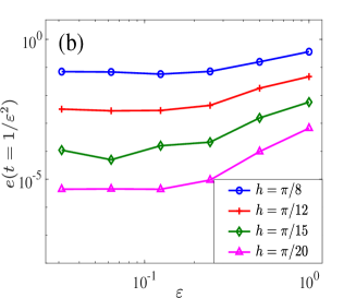
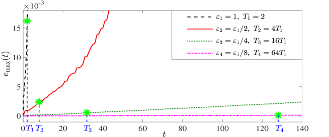
Refer to caption

Figure 1: Long-time temporal errors for the wave function of the TSFP method for the NLDE (1.0.1) in 1D with different ε𝜀\varepsilon.

Refer to caption

Refer to caption

Figure 2: Long-time spatial errors of the TSFP method for the NLDE (1.0.1) in 1D at t=1/ε2𝑡1superscript𝜀2t=1/\varepsilon^{2}.

Refer to caption

Refer to caption

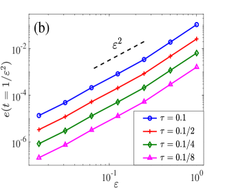
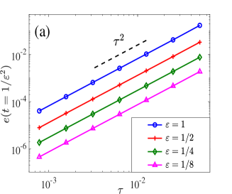
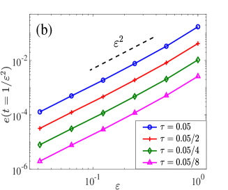
Figure 3: Long-time temporal errors of the TSFP method for the NLDE (1.0.1) in 1D at t=1/ε2𝑡1superscript𝜀2t=1/\varepsilon^{2}.

Refer to caption

Refer to caption

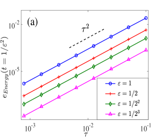
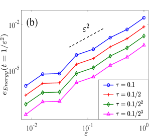
Figure 4: Long-time error for the discretized energy Ehnsubscriptsuperscript𝐸𝑛E^{n}_{h} of the TSFP method for the NLDE (1.0.1) in 1D at t=1/ε2𝑡1superscript𝜀2t=1/\varepsilon^{2}.

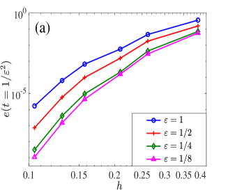
Fig. 1 displays the long-time errors of the TSFP method (2.2.18) for the NLDE (1.0.1) in 1D with different ε𝜀\varepsilon, which confirms the improved uniform error bounds at O(ε2τ2)𝑂superscript𝜀2superscript𝜏2O(\varepsilon^{2}\tau^{2}) up to the time at O(1/ε2)𝑂1superscript𝜀2O(1/\varepsilon^{2}). Fig. 2 & Fig. 3 show the spatial and temporal errors of the TSFP methods for the NLDE (1.0.1) in 1D at t=1/ε2𝑡1superscript𝜀2t=1/\varepsilon^{2}, respectively. Fig. 2 indicates the spectral accuracy of the TSFP method in space and the spatial errors are independent of the parameter ε𝜀\varepsilon. From Fig. 3 (a), we observe the second-order convergence of the TSFP method in time for the fixed ε𝜀\varepsilon. Fig. 3 (b) again validates that the long-time errors behave like O(ε2τ2)𝑂superscript𝜀2superscript𝜏2O(\varepsilon^{2}\tau^{2}) up to the time at O(1/ε2)𝑂1superscript𝜀2O(1/\varepsilon^{2}). Fig. 4 shows the error of the discrete energy Ehnsubscriptsuperscript𝐸𝑛E^{n}_{h} also behaves like O(ε2τ2)𝑂superscript𝜀2superscript𝜏2O(\varepsilon^{2}\tau^{2}) up to the time at O(1/ε2)𝑂1superscript𝜀2O(1/\varepsilon^{2}).

4.2 The long-time dynamics in 2D

In this subsection, we show an example in 2D with the irrational aspect ratio of the domain (x,y)(0,2π)×(0,1)𝑥𝑦02𝜋01(x,y)\in(0,2\pi)\times(0,1). In the numerical experiment, we choose the initial data as

ϕ1(0,x)=sin(2x)+sin(2πy),ϕ2(0,x)=11+cos2(2x)+cos(2πy).formulae-sequencesubscriptitalic-ϕ10𝑥2𝑥2𝜋𝑦subscriptitalic-ϕ20𝑥11superscript22𝑥2𝜋𝑦\phi_{1}(0,x)=\sin(2x)+\sin(2\pi y),\quad\phi_{2}(0,x)=\frac{1}{1+\cos^{2}(2x)}+\cos(2\pi y). (4.2.69)

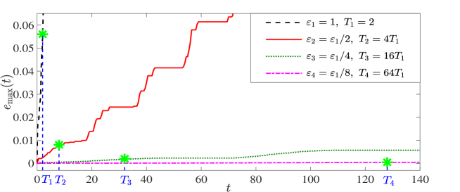
Refer to caption

Figure 5: Long-time temporal errors of the TSFP method for the NLDE (1.0.1) in 2D with different ε𝜀\varepsilon.

Refer to caption

Refer to caption

Figure 6: Long-time temporal errors of the TSFP method for the NLDE (1.0.1) in 2D at t=1/ε2𝑡1superscript𝜀2t=1/\varepsilon^{2}.

Fig. 5 presents the long-time errors of the TSFP method for the NLDE (1.0.1) in 2D with a fixed time step τ𝜏\tau and different ε𝜀\varepsilon, which confirms the improved uniform error bounds in 2D. Fig. 6 plots the temporal errors of the TSFP method for the NLDE in 2D at t=1/ε2𝑡1superscript𝜀2t=1/\varepsilon^{2}, which indicates the second-order convergence in time and again validates the improved uniform error bounds at O(ε2τ2)𝑂superscript𝜀2superscript𝜏2O(\varepsilon^{2}\tau^{2}) up to the time at O(1/ε2)𝑂1superscript𝜀2O(1/\varepsilon^{2}).

4.3 Extension to the oscillatory NLDE

In this subsection, we extend the TSFP method and error estimates to an oscillatory NLDE which propagates waves with wave length at O(ε2)𝑂superscript𝜀2O(\varepsilon^{2}) in time and wave speed at O(ε2)𝑂superscript𝜀2O(\varepsilon^{-2}) in space. Introduce a re-scale in time s=ε2t𝑠superscript𝜀2𝑡s=\varepsilon^{2}t and Φ~(s,𝐱)=Φ(t,𝐱)~Φ𝑠𝐱Φ𝑡𝐱\widetilde{\Phi}(s,{\bf x})=\Phi(t,{\bf x}), then the NLDE (1.0.1) could be reformulated into the following oscillatory NLDE

isΦ~=1ε2[ij=1dσjj+σ3]Φ~+𝐅(Φ~)Φ~xΩ,t>0,formulae-sequence𝑖subscript𝑠~Φ1superscript𝜀2delimited-[]𝑖superscriptsubscript𝑗1𝑑subscript𝜎𝑗subscript𝑗subscript𝜎3~Φ𝐅~Φ~Φformulae-sequence𝑥Ω𝑡0i\partial_{s}\widetilde{\Phi}=\frac{1}{\varepsilon^{2}}\Big{[}-i\sum_{j=1}^{d}\sigma_{j}\partial_{j}+\sigma_{3}\Big{]}\widetilde{\Phi}+{{\bf F}}(\widetilde{\Phi})\widetilde{\Phi}\quad x\in\Omega,\quad t>0, (4.3.70)

with the initial data

Φ~(s=0,𝐱)=Φ~0(𝐱)=O(1),𝐱Ω¯.formulae-sequence~Φ𝑠0𝐱subscript~Φ0𝐱𝑂1𝐱¯Ω\widetilde{\Phi}(s=0,{\bf x})=\widetilde{\Phi}_{0}({\bf x})=O(1),\quad{\bf x}\in\overline{\Omega}. (4.3.71)

The solution of the oscillatory NLDE (4.3.70) propagates waves with amplitude at O(1)𝑂1O(1), wavelength at O(1)𝑂1O(1) and O(ε2)𝑂superscript𝜀2O(\varepsilon^{2}) in space and time, respectively, and wave speed at O(ε2)𝑂superscript𝜀2O(\varepsilon^{-2}) in space. We remark here the oscillatory nature of the NLDE (4.3.70) is quite different from the NLDE in the nonrelativistic limit regime, which has been widely studied in Bao et al. (2016), Cai & Wang (2019), Hunziker (1975), Krämer et al. (2019) and Lemou et al. (2017). In fact, in this regime, the wave speed is at O(1/ε2)𝑂1superscript𝜀2O(1/\varepsilon^{2}), while the NLDE in the nonrelativistic limit regime propagates waves with wave speed at O(1)𝑂1O(1). According to the time rescaling, by taking the time step κ=ε2τ𝜅superscript𝜀2𝜏\kappa=\varepsilon^{2}\tau, we could extend the improved error bounds on the TSFP method for the long-time problem to the oscillatory NLDE (4.3.70) up to the fixed time T𝑇T. We also just present the result in 1D and it is straightforward to extend to 2D and 3D cases.

Theorem 4.1

Let Φ~nsuperscript~Φ𝑛\widetilde{\Phi}^{n} be the numerical approximation obtained from the TSFP method for the oscillatory NLDE (4.3.70) in 1D. Assume the exact solution Φ~(s,x)~Φ𝑠𝑥\widetilde{\Phi}(s,x) satisfies

Φ~(s,x)L([0,T];(Hm(Ω))2),m3,formulae-sequence~Φ𝑠𝑥superscript𝐿0𝑇superscriptsuperscript𝐻𝑚Ω2𝑚3\widetilde{\Phi}(s,x)\in{L^{\infty}([0,T];(H^{m}(\Omega))^{2})},\quad m\geq 3,

then there exist h0>0subscript00h_{0}>0 and 0<κ0<10subscript𝜅010<\kappa_{0}<1 sufficiently small and independent of ε𝜀\varepsilon such that for any 0<ε10𝜀10<\varepsilon\leq 1, when 0<hh00subscript00<h\leq h_{0} and 0<κε2ακ00𝜅superscript𝜀2𝛼subscript𝜅00<\kappa\leq\varepsilon^{2}\alpha\kappa_{0} for a fixed constant α(0,1)𝛼01\alpha\in(0,1), the following improved uniform error bounds hold

Φ~(sn,x)IMΦ~nH1hm1+κ2ε2+κ0m1,0nTκ.formulae-sequenceless-than-or-similar-tosubscriptnorm~Φsubscript𝑠𝑛𝑥subscript𝐼𝑀superscript~Φ𝑛superscript𝐻1superscript𝑚1superscript𝜅2superscript𝜀2superscriptsubscript𝜅0𝑚10𝑛𝑇𝜅\left\|\widetilde{\Phi}(s_{n},x)-I_{M}\widetilde{\Phi}^{n}\right\|_{H^{1}}\lesssim h^{m-1}+\frac{\kappa^{2}}{\varepsilon^{2}}+\kappa_{0}^{m-1},\quad 0\leq n\leq\frac{T}{\kappa}. (4.3.72)

In particular, if the exact solution is sufficiently smooth, e.g. Φ~(t,x)(H)2~Φ𝑡𝑥superscriptsuperscript𝐻2\widetilde{\Phi}(t,x)\in(H^{\infty})^{2}, the improved uniform error bounds for small κ0subscript𝜅0\kappa_{0} would become

Φ~(sn,x)IMΦ~nH1hm1+κ2ε2,0nTκ.formulae-sequenceless-than-or-similar-tosubscriptnorm~Φsubscript𝑠𝑛𝑥subscript𝐼𝑀superscript~Φ𝑛superscript𝐻1superscript𝑚1superscript𝜅2superscript𝜀20𝑛𝑇𝜅\left\|\widetilde{\Phi}(s_{n},x)-I_{M}\widetilde{\Phi}^{n}\right\|_{H^{1}}\lesssim h^{m-1}+\frac{\kappa^{2}}{\varepsilon^{2}},\quad 0\leq n\leq\frac{T}{\kappa}. (4.3.73)

The proof of the improved error bounds for the oscillatory NLDE (4.3.70) in Theorem 4.3.73 is quite similar to the long-time problem. We omit the details here for brevity and present some numerical results to confirm the sharpness of the improved error bounds. The initial data is chosen as

ϕ~1(0,x)=4x4(1x)4+2,ϕ~2(0,x)=4x4(1x)4,x(0,1).formulae-sequencesubscript~italic-ϕ10𝑥4superscript𝑥4superscript1𝑥42formulae-sequencesubscript~italic-ϕ20𝑥4superscript𝑥4superscript1𝑥4𝑥01\widetilde{\phi}_{1}(0,x)=4x^{4}(1-x)^{4}+2,\quad\widetilde{\phi}_{2}(0,x)=4x^{4}(1-x)^{4},\quad x\in(0,1). (4.3.74)

The regularity is enough to ensure the improved error bounds.

Table 1: Temporal errors of the TSFP method for the NLDE (4.3.70) in 1D at t=1𝑡1t=1.
e(t=1)𝑒𝑡1e(t=1) κ0=0.05subscript𝜅00.05\kappa_{0}=0.05 κ0/4subscript𝜅04\kappa_{0}/4 κ0/42subscript𝜅0superscript42\kappa_{0}/4^{2} κ0/43subscript𝜅0superscript43\kappa_{0}/4^{3} κ0/44subscript𝜅0superscript44\kappa_{0}/4^{4}
ε0=1subscript𝜀01\varepsilon_{0}=1 1.26E-2 7.57E-4 4.72E-5 2.95E-6 1.84E-7
order - 2.03 2.00 2.00 2.00
ε0/2subscript𝜀02\varepsilon_{0}/2 1.21E-1 5.71E-3 3.52E-4 2.20E-5 1.37E-6
order - 2.20 2.01 2.00 2.00
ε0/22subscript𝜀0superscript22\varepsilon_{0}/2^{2} 5.39E-2 9.18E-3 3.85E-4 2.37E-5 1.48E-6
order - 1.23 2.29 2.01 2.00
ε0/23subscript𝜀0superscript23\varepsilon_{0}/2^{3} 2.40E-1 1.08E-2 2.13E-3 8.68E-5 5.34E-6
order - 2.24 1.17 2.31 2.01
ε0/24subscript𝜀0superscript24\varepsilon_{0}/2^{4} 1.17E-1 3.80E-2 2.46E-3 6.76E-4 2.46E-5
order - 0.81 1.97 0.93 2.39

Table 1 lists the temporal errors of the TSFP method for the oscillatory NLDE (4.3.70) in 1D with different ε𝜀\varepsilon. It can be clearly observed that the second-order convergence can only be observed when κε2less-than-or-similar-to𝜅superscript𝜀2\kappa\lesssim\varepsilon^{2} (cf. the upper triangle above the diagonal with bold letters) and the temporal errors behave like O(κ2/ε2)𝑂superscript𝜅2superscript𝜀2O(\kappa^{2}/\varepsilon^{2}). Along each diagonal in the table, i.e. with κ=O(ε2)𝜅𝑂superscript𝜀2\kappa=O(\varepsilon^{2}), we observe linear convergence with respect to κ𝜅\kappa, which confirm the error bound at κ2ε2=O(κ2κ)=O(κ)superscript𝜅2superscript𝜀2𝑂superscript𝜅2𝜅𝑂𝜅\frac{\kappa^{2}}{\varepsilon^{2}}=O\left(\frac{\kappa^{2}}{\kappa}\right)=O(\kappa) in (4.3.73).

5 Conclusions

Improved uniform error bounds on time-splitting methods for the long-time dynamics of the weakly nonlinear Dirac equation (NLDE) were rigorously proven. With the help of the regularity compensation oscillation (RCO) technique, the long-time errors up to the time at O(1/ε2)𝑂1superscript𝜀2O(1/\varepsilon^{2}) for the semi-discretization and full-discretization are at O(ε2τ2)𝑂superscript𝜀2superscript𝜏2O(\varepsilon^{2}\tau^{2}) and O(hm1+ε2τ2)𝑂superscript𝑚1superscript𝜀2superscript𝜏2O(h^{m-1}+\varepsilon^{2}\tau^{2}), respectively, which improve the standard error bounds in the literature at O(τ2)𝑂superscript𝜏2O(\tau^{2}) and O(hm1+τ2)𝑂superscript𝑚1superscript𝜏2O(h^{m-1}+\tau^{2}) for the semi-discretization and full-discretization, respectively, especially when 0<ε10𝜀much-less-than10<\varepsilon\ll 1. The improved error bounds were extended to an oscillatory NLDE up to a fixed time T𝑇T. Numerical results in 1D and 2D agreed well with the theoretical results and suggested that the error bounds are sharp.

Acknowledgements

This work was partially supported by the Ministry of Education of Singapore grant MOE2019-T2-1-063 (R-146-000-296-112, W. Bao, Y. Feng) and Natural Science Foundation of China grant 12171041 and 11771036 (Y. Cai).

References

  • Balabane et al. (1988) Balabane, M., Cazenave, T., Douady, A. & Merle, F. (1988) Existence of excited states for a nonlinear Dirac field. Commun. Math. Phys., 119, 153–176.
  • Bao et al. (2017) Bao, W., Cai, Y., Jia, X. & Tang, Q. (2017) Numerical methods and comparison for the Dirac equation in the nonrelativistic limit regime. J. Sci. Comput., 71, 1094 –1134.
  • Bao et al. (2016) Bao, W., Cai, Y., Jia, X. & Yin, J. (2016) Error estimates of numerical methods for the nonlinear Dirac equation in the nonrelativistic limit regime. Sci. China Math., 59, 1461–1494.
  • Bao et al. (2021a) Bao, W., Cai, Y. & Feng, Y. (2021) Improved uniform error bounds for the time-splitting methods for the long-time dynamics of the Schrödinger/nonlinear Schrödinger equation. arXiv: 2109.08940.
  • Bao et al. (2021b) Bao, W., Cai, Y. & Feng, Y. (2021) Improved uniform error bounds on time-splitting methods for the long-time dynamics of the nonlinear Klein–Gordon equation with weak nonlinearity. arXiv:2109.14902.
  • Bao et al. (2020) Bao, W., Cai, Y. & Yin, J. (2020) Super-resolution of time-splitting methods for the Dirac equation in the nonrelativistic regime. Math. Comp., 89, 2141–2173.
  • Bao et al. (2021c) Bao, W., Cai, Y. & Yin, J. (2021) Uniform error bounds of time-splitting methods for the nonlinear Dirac equation in the nonrelativistic limit regime. SIAM J. Numer. Anal., 59, 1040–1066.
  • Bao et al. (2021d) Bao, W., Feng, Y. & Yin, J. (2021) Improved uniform error bounds on time-splitting methods for the long-time dynamics of the Dirac equation with small potentials. arXiv: 2112.03616.
  • Bao & Yin (2019) Bao, W. & Yin, J. (2019) A fourth-order compact time-splitting Fourier pseudospectral method for the Dirac equation. Res. Math. Sci., 6, Paper No. 11, 35.
  • Bartsch & Ding (2006) Bartsch, T. & Ding, Y. (2006) Solutions of nonlinear Dirac equations. J. Diff. Eq., 226, 210–249.
  • Brinkman et al. (2014) Brinkman, D., Heitzinger, C. & Markowich, P. A. (2014) A convergent 2D finite-difference scheme for the Dirac-Poisson system and the simulation of graphene. J. Comput. Phys., 257, 318–332.
  • Cai & Wang (2019) Cai, Y. & Wang, Y. (2019) Uniformly accurate nested Picard iterative integrators for the Dirac equation in the nonrelativistic limit regime. SIAM J. Numer. Anal., 57, 1602–1624.
  • Cazenave & Vazquez (1986) Cazenave, T. & Vazquez, L. (1986) Existence of localized solutions for a classical nonlinear Dirac field. Commun. Math. Phys., 105, 35–47.
  • Chang et al. (1975) Chang, S. J., Ellis, S. D. & Lee, B. W. (1975) Chiral confinement: An exact solution of the massive Thirring model. Phy. Rev. D, 11, 3572–3582.
  • Chartier et al. (2016) Chartier, P., Méhats, F., Thalhammer, M. & Zhang, Y. (2016) Improved error estimates for splitting methods applied to highly-oscillatory nonlinear Schrödinger equations. Math. Comp., 85, 2863–2885.
  • De Frutos & Sanz-Serna (1989) De Frutos, J. & Sanz-Serna, J. M. (1989) Split-step spectral schemes for nonlinear Dirac systems. J. Comput. Phys., 83, 407–423.
  • Dirac (1928) Dirac, P. A. M. (1928) The quantum theory of the electron. Proc. R. Soc. Lond., A 117, 610–624.
  • Dirac (1958) Dirac, P. A. M. (1958) Principles of Quantum Mechanics. London: Oxford University Press.
  • Esteban & Séré (1997) Esteban, M. J. & Séré, E. (1997) Existence and multiplicity of solutions for linear and nonlinear Dirac problems. Partial Differential equations and their applications (Toronto, ON, 1995), CRM Proc. Lecture Notes, vol. 12, Amer. Math. Soc., Providence, RI., 107–118.
  • Faou & Greébert (2011) Faou, E. & Greébert, B. (2011) Hamiltonian interpolation of splitting approximations for nonlinear PDEs. Found. Comput. Math., 11, 381–415.
  • Faou et al. (2011) Faou, E., Greébert, B. & Paturel, E. (2010) Birkhoff normal form for splitting methods applied to semilinear Hamiltonian PDEs. Part II: Abstract splitting. Numer. Math., 114, 459–490.
  • Fefferman & Weistein (2012) Fefferman, C. L. & Weistein. M. I. (2012) Honeycomb lattice potentials and Dirac points. J. Amer. Math. Soc., 25, 1169–1220.
  • Feng & Yin (2021) Feng, Y. & Yin, J. (2021) Spatial resolution of different discretizations over long-time for the Dirac equation with small potentials. arXiv: 2105.10468.
  • Feng et al. (2022) Feng, Y., Xu, Z. & Yin, J. (2022) Uniform error bounds of exponential wave integrator methods for the long-time dynamics of the Dirac equation with small potentials. Appl. Numer. Math., 172, 50–66.
  • Fillion-Gourdeau et al. (2012) Fillion-Gourdeau, F., Lorin, E. & Bandrauk, A. D. (2012) Numerical solution of the time-dependent Dirac equation in coordinate space without fermion-doubling. Comput. Phys. Commun., 183, 1403–1415.
  • Fushchich & Shtelen (1983) Fushchich, W. I. & Shtelen, W. M. (1983) On some exact solutions of the nonlinear Dirac equation. J. Phys. A: Math Gen, 16, 271–277.
  • Fushchich & Zhdanov (1989) Fushchich, W. I. & Zhdanov, R. Z. (1989) Symmetry and exact solutions of nonlinear spinor equations. Phys. Rep., 172, 123–174.
  • Gauckler & Lubich (2010) Gauckler, L. & Lubich, C. (2010) Splitting integrators for nonlinear Schrödinger equations over long times. Found. Comput. Math., 10, 275–302.
  • Haddad & Carr (2009) Haddad, L. H. & Carr, L. D. (2009) The nonlinear Dirac equation in Bose-Einstein condensates: Foundation and symmetries. Phys. D, 238, 1413–1421.
  • Hairer & Lubich (2009) Hairer, E. & Lubich, C. (2008) Spectral semi-discretisations of weakly nonlinear wave equations over long times. Found. Comput. Math., 8, 319–334.
  • Hunziker (1975) Hunziker, W. (1975) On the nonrelativistic limit of the Dirac theory. Commun. Math. Phys., 40, 215–222.
  • Komech & Komech (2010) Komech, A. & Komech, A. (2010) Global attraction to solitary waves for a nonlinear Dirac equation with mean field interaction. SIAM J. Math. Anal., 42, 2944–2964.
  • Krämer et al. (2019) Krämer, P., Schratz, K. & Zhao, X. (2019) Splitting methods for nonlinear Dirac equations with Thirring type interaction in the nonrelativistic limit regime. J. Comput. Appl. Math., 387, 112494.
  • Lemou et al. (2017) Lemou, M., Méhats, F. & Zhao, X. (2017) Uniformly accurate numerical schemes for the nonlinear Dirac equation in the nonrelativistic limit regime. Commun. Math. Sci., 15, 1107–1128.
  • Lubich (2008) Lubich, C. (2008) On splitting methods for Schrödinger-Poisson and cubic nonlinear Schrödinger equations. Math. Comp., 77, 2141–2153.
  • Mathieu (1985) Mathieu, P. (1985) Soliton solutions for Dirac equations with homogeneous non-linearity in (1+1) dimensions. J. Phys. A: Math. Gen., 18, L1061–L1066.
  • McLachlan & Quispel (2002) McLachlan, R. I. & Quispel, G. R. W., Splitting methods. Acta Numer., 11, 341–434.
  • Pecher (2014) Pecher, H. (2014) Local well-posedness for the nonlinear Dirac equation in two space dimensions. Commun. Pure Appl. Anal., 13, 673–685.
  • Rafflski (1977) Rafflski, J. (1977) Soliton solutions of a selfinteracting Dirac field in three space dimensions. Phys. Lett. B, 66, 262–266.
  • Sasaki (2015) Sasaki, H. (2015) Small data scattering for the one-dimensional nonlinear Dirac equation with power nonlinearity. Comm. Partial Differential Equations, 40, 1959–2004.
  • Shen et al. (2011) Shen, J., Tang, T. & Wang, L.-L. (2011) Spectral Methods: Algorithms, Analysis and Applications. Berlin, Heidelberg: Springer-Verlag.
  • Soler (1970) Soler, M. (1970) Classical, stable, nonlinear spinor field with positive rest energy. Phys. Rev. D, 1, 2766-2769.
  • Strang (1968) Strang, G. (1968) On the construction and comparison of difference schemes. SIAM J. Numer. Anal., 5, 505–517.
  • Takahashi (1979) Takahashi, K. (1979) Soliton solutions of nonlinear Dirac equations. J. Math. Phys., 20, 1232–1238.
  • Thirring (1958) Thirring, W. E. (1958) A soluble relativistic field theory. Ann. Phys., 3, 91–112.
  • Trotter (1959) Trotter, H. F. (1959) On the product of semi-groups of operator. Proc. Amer. Math. Soc., 10, 545–551.