Global Gravity Field Model from Taiji-1 Observations

Abstract

Taiji-1 is the first technology demonstration satellite of the Taiji program of China’s space-borne gravitational wave antenna. After the demonstration of the key individual technologies, Taiji-1 continues collecting the data of the precision orbit determinations, satellite attitudes, and non-conservative forces exerted on the S/C. Therefore, during its free-fall, Taiji-1 can be viewed as operating in the high-low satellite-to-satellite tracking mode of a gravity recovery mission. In this work, we have selected and analyzed the one month data from Taiji-1’s observations, and developed the techniques to resolve the long term interruptions and disturbances in the data due to the scheduled technology demonstration experiments. The first global gravity model TJGM-r1911, that independently derived from China’s own satellite mission, is successfully built from Taiji-1’s observations. Compared with gravity models from CHAMP and other satellite gravity missions, the accuracy discrepancies exist, which is mainly caused by the data discontinuity problem. As the extended free-falling phase been approved, Taiji-1 could serve as a gravity recovery mission for China since 2022 and it will provide us the independent measurement of both the static and the monthly time-variable global gravity field.

I Introduction

In 2000, Chinese Academy of Sciences (CAS) established China’s first working group of the space borne gravitational wave observatories that led by Academician Wen-Rui Hu. China had then started her own journey to gravitational wave detections in space and joined the international corporations led by the LISA team Danzmann (2011). Motivated mainly by the concept of ALIA mission Bender (2004), China’s first concept of space borne gravitational wave antennas was proposed in 2011 Gong et al. (2011), and afterward, a more conservative design was made Gong et al. (2015); Xue-fei et al. (2015). In 2016, the breaking news of the first detection of gravitational wave The LIGO Scientific Collaboration et al. (2015); Abbott et al. (2016a, b, c) was announced by the Adv-LIGO team, which was soon recognized as one of the most significant achievements in this new century of general relativity. The subsequent gravitational wave detections by the LIGO-VIRGO collaboration had then raised the curtain of the new era of gravitational wave astronomy and astrophysics, and also boosted the progress of the space missions. Along with such breakthroughs, and also being encouraged by the successful experiments of the LISA Pathfinder mission Armano et al. (2016, 2018, 2019); Armano (2019); Anderson et al. (2018), the Taiji program in space was released by CAS in 2016 Cyranoski (2016); Hu and Wu (2017) which outlined its 3-step R&D roadmap for China’s space gravitational wave antenna in the future Luo et al. (2020a, b). The ultimate goal of this program is the Taiji mission, a heliocentric LISA-like mission that expected to be launched in the early 2030s. Consisting of three space-crafts (S/C), the Taiji mission will be an almost equilateral triangular constellation with the arm-length about $3\times 10^{6}$ km and the sensitive band ranging from 0.1 mHz to 1 Hz. The scientific objectives will include such gravitational wave sources as coalescing supermassive black hole binaries, extreme mass ratio inspirals, stochastic gravitational wave backgrounds, etc. Hu and Wu (2017); Ruan et al. (2020a); Luo et al. (2020a, b); The Taiji Scientific Collaboration et al. (2021); Ruan et al. (2020b, 2021); Wang et al. (2021a, b).

With the phase A study started in May 2018 and the ground-based tests of related technologies Liu et al. (2018a, b); Li et al. (2018, 2019, 2020); Liu et al. (2021), the Taiji-1 mission, as the first technology demonstration satellite of the Taiji program, was approved by CAS in August 2018. The detailed design was finished in October 2018 and all the unit flight models were delivered before APR 2019. The assembly integrations and tests were then conducted from APR 2019, and in August 2019 Taiji-1 was launched. The most important individual technologies of China’s space gravitational wave antenna were verified in space, including gravitational reference sensors (GRS), high precision laser interferometers, drag-free control system, $\mu$-N thrusters, and the ultra-stable and clean platform. The successful operation of Taiji-1 had demonstrated and confirmed the designed performances of the scientific payloads and the satellite platform The Taiji Scientific Collaboration (2021); The Taiji Scientific Collaboration et al. (2021). In 2022, the Taiji-1 satellite has entered into its final extended phase, and the challenging experiment on global gravity recoveries will be carried out.

The orbital dynamics of Taiji-1 is determined by the forces acting on the S/C, which, due to their physical origins, can be divided into three classes: the gravitational forces including the almost centripetal force from the Earth and the perturbations from the Sun, the Moon and other celestial bodies, the non-conservative forces from the space environments such as air drags, Solar radiation pressure Earth albedo, and also the disturbances from thruster events. During its science operation, Taiji-1 has continuously collected the precision orbit determination (POD) data based on the Global Navigation Satellite Systems (GPS and BeiDou), the satellite attitude data from star sensors, and also the precision measurements by the GRS of the non-conservative forces exerted on the S/C. Therefore, given such observation data, the detailed information of the Earth gravitational field could be inferred based on the satellite dynamic model.

From this point of view, apart from the disruptions by the technology demonstration experiments such as the thruster performance tests, the drag-free control tests, the satellite maneuvers and so on, the free-falling mode of the Taiji-1 satellite can be viewed as the high-low Satellite-to-Satellite Tracking (hl-SST) mode of the Earth gravity recovery mission Moore et al. (2003); Naeimi and Flury (2017); Reigber (2005). See Fig. 1 for illustration.

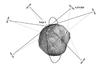
Figure 1: The illustration of the high-low satellite-to-satellite tracking mode of Taiji-1.

Taiji-1 could then serve as a gravity recovery satellite for China, which could provide us the independent measurements of both the static global gravity field over about one year and the monthly averaged time-variable gravity field of long wavelengths.

The gravity model obtained from Taiji-1, as the tentative data products, could then fuse with the up-coming geopotential measurements from the official Low-Low SST gravity recovery mission of China’s satellite gravity program. Further, such precedent data products could also provide the opportunity to make valuable cross-validations between the two missions. Based on such considerations, the Taiji team had approved the extended free-falling phase of Taiji-1 in the end of 2021, and the satellite is to follow its geodesic orbit around Earth with minimal disruptions and disturbances only from events as attitude adjustments, etc.

In this work, we introduce the first Earth gravity field product obtained from Taiji-1’s observations during its science operation. The conventional energy integral method employed in gravity recoveries for hl-SST missions is outline in Sec. II. Since the free-falling motion of the S/C in Earth’s gravitational field and the continual observations of the orbit and non-conservative forces are crucial to the global gravity recoveries, the data set is carefully selected to avoid the disruptions and gaps as much as possible. The measurement data from Taiji-1 and the ancillary models required are described in Sec. III. While the interruptions and the anomalies still exist in the chosen data, the software package TJGrav is developed to resolve such problems and to process the data. The data fusion techniques are developed to synthesize the measurement data with certain models that are calibrated carefully by the measurements. The data processing procedure can be found in Sec. IV.The first monthly Earth gravity model TJGM-r1911 independently derived from China’s own satellite mission Taiji-1 is discussed in Sec. V. Conclusions and an outlook are provided in Sec. VI.

II Energy integral method

Proposed by O’keefe in O’Keefe (1957) firstly and investigated in detail in Hotine and Morrison (1969); Wolff (1969); Jekeli (1999); Visser et al. (2003), the energy integral or the energy balance approach, has been developed as a full-fledged and widely used method in the global gravity inversions for hl-SST satellite gravity missions. It is based on the theoretical prediction that ideally the Jacobi’s integral of a S/C motion is conserved along its orbits Jacobi (1836), which can be viewed as an equivalent to the conservation of total mechanical energy. Therefore, the balance between the kinetic energy and the gravitational energy of the S/C can be used to derive the detailed information of the gravity field, given the measured data of the S/C position and velocity.

The key to the approach in realistic applications is to account for the energy dissipation caused by the non-conservative surface forces acting on the S/C accurately. Generally, low Earth orbits are adopted for the satellite gravity missions, and the main contributions to the total non-conservative force include the air drags, the solar radiation pressures and also the Earth albedo pressure. One can use force models to reduce the errors caused by such energy loss, while the precise and real time measurements of such perturbation forces will greatly improve the fitting accuracy of the gravity field. Please see Visser et al. (2003); Gerlach et al. (2003a, b); Moore et al. (2003); Foldvary et al. (2005); Jaggi et al. (2011) for the detailed discussions of the energy integral method and its applications to the CHAMP, GRACE and GOCE missions.

Here, we outline the theoretical principle of the energy integral method and give the necessary definitions used in this work. The functional model chosen here to estimate the geopotential $V$ is the following spherical harmonic series truncated at maximum degree $N$ and defined in the Earth centered spherical coordinates system $\{r,\theta,\lambda\}$ (radius, geocentric latitude, longitude),

$$V\left(r,\theta,\lambda\right)=\frac{GM}{r}\left[1+\sum_{n=2}^{N}\sum_{m=-n}^{n}A_{nm}\left(\frac{R}{r}\right)^{n}Y_{nm}\left(\theta,\lambda\right)\right],$$ (1)

where $G$ is the gravitational constant, $M$ the total mass of the Earth, and $R$ the mean equatorial radius. $Y_{nm}$ denotes the surface spherical harmonics of degree $n$ and order $m$

$$Y_{nm}(\vartheta,\lambda)=\bar{P}_{n\lvert m\rvert}(\sin\theta)\begin{cases}\cos m\lambda&m\geq 0\\ \sin\lvert m\rvert\lambda&m<0,\end{cases}$$ (2)

where $\bar{P}_{nm}$ is the fully normalized associated Legendre function of degree $n$ and order $m$, and $A_{nm}=\{C_{nm},S_{nm}\}$, with $C_{nm}$ for $m\geq 0$ and $S_{nm}$ for $m<0$, are the unknown spherical harmonic coefficients to be determined.

The Earth gravity field, in terms of the geopotential coefficients $A_{mn}$, could be obtained from the least-square solutions of the observation equations that link the orbit position and velocity solutions to the gravity field unknowns. The energy integral is used to derive the observation equations, which is defined along the S/C orbit as

$$V=V_{0}+\int_{t_{0}}^{t}\bm{g}\cdot\bm{\dot{r}}d\tau,$$ (3)

where $V$ and $V_{0}$ are the Earth geopotentials at the S/C orbit positions of time $t$ and $t_{0}$ respectively, $\bm{r}$ and $\dot{\bm{r}}$ the position and velocity vector of the S/C in the Earth-centered and Earth-fixed reference frame. The vector $\bm{g}$ denotes the acceleration caused by static geopotentials of the Earth

$$\bm{g}=\bm{\ddot{r}}+2\bm{\omega}\times\bm{\dot{r}}+\bm{\omega}\times\left(\bm{\omega}\times\bm{r}\right)-\bm{a_{NC}-a_{G},}$$ (4)

where $\bm{\omega}$ is the angular velocity of the Earth rotation. $\bm{a_{NC}}$ includes all the non-gravitational accelerations exerted by the satellite, and $\bm{a}_{\bm{G}}$ counts for all the perturbations from other time-varying gravitational sources such as tides, mass transfers in atmosphere and ocean, and 3rd-body effects from the Sun or the Moon. To resolve the long wavelength or low-degree gravity field, we split the Earth geopotentials into three parts $U$, $V_{l}$ and $V_{h}$, where $U$ represents the monopole potential, $V_{l}$ is the potential consisting of low-degree harmonics and $V_{h}$ the one from high-degree harmonics. Thus, Eq.3 becomes

$$H+V_{l}\left(\bm{r}\right)= \frac{1}{2}\mathbf{\dot{r}}\cdot\mathbf{\dot{r}}-\frac{1}{2}\left(\bm{\omega}\times\bm{r}\right)\cdot\left(\bm{\omega}\times\bm{r}\right)$$

$$-\int_{t_{0}}^{t}\bm{a_{NC}}\cdot\mathbf{\dot{r}}\mathrm{d}\tau-\int_{t_{0}}^{t}\bm{a_{G}}\cdot\mathbf{\dot{r}}\mathrm{d}\tau-U-V_{h}$$ (5)

The unknown integration constant $H$ and the coefficients $\{C_{nm},\ S_{nm}\}$ of the low-degree components on the left-hand side of Eq. 5 are to be resolved with Taiji-1’s observations and the modeled ancillary data substituted into the right-hand side of the equation.

III Data sets and ancillary models

III.1 Data sets

The Taiji-1 satellite was launched to a circular Sun-synchronous dawn/dusk orbit with the altitude about $600\ km$ and inclination angle $97.67^{o}$. The orbit has a stable Sun-facing angle, which can provide a constant power supply for the battery and also the stable temperature gradient for the platform. The satellite is about 180 kg, and along such orbit, the solar radiation pressure contributes to the non-conservative forces dominantly, and the air drags along the orbit turns out to be small. One of the key payloads of Taiji-1 is the GRS installed at the mass center of the S/C. Except for the drag-free control experiments during the science operation, where the satellite is controlled to trace the motions of the test mass inside the GRS along the radial direction, the GRS are set to work in the accelerometer mode in most cases. The electrostatic actuation forces keeping the test mass to follow the motions of the S/C will then provide the precise measurements of the non-gravitational forces exerted by the S/C.

The data products needed for the Earth gravity recoveries include the POD data from both the GPS and BeiDou (BD) systems, the GRS data of the non-gravitational forces measured in the satellite frame and the S/C attitude data to transform the physical measurements from the satellite frame to the inertial reference frame. In this work, our first Taiji-1 gravity model is based on the data from 01-11-2019 to 31-11-2019. As mentioned, during this month fewer experiments related to the GRS, the thrusters, and the satellite-maneuvers were performed. The S/C maintained steadily in the Earth pointing attitude and the POD data is in good quality. The one-month data length was chosen since any extension could hardly improve the final fitting accuracy due to the frequent disruptions and gaps in the data from the technology demonstration experiments. Further, since the monthly measurements of the time-variable gravity field from Taiji-1’s extended free-falling phase is under preparation, this first monthly gravity model could serve as a reference.

The orbit precision of Taiji-1 is determined by the Global Navigation Satellite Systems, including both the GPS and the BD system. The POD data from GPS and BD are both defined in the Earth-centered and Earth-fixed reference frame with the sampling rate of 1 Hz. The amplitude spectrum density (ASD) of the POD data including the positions and the velocities of Taiji-1 are shown in Fig. 2. In most cases, the Taiji-1 satellite can be more often tracked by GPS satellites than by the BD satellites. Fig. 3 shows the difference between the measurements from BD and GPS.

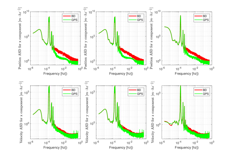
Figure 2: ASDs of Taiji-1’s POD data from both GPS and BD in the Earth-centered and Earth-fixed reference frame.

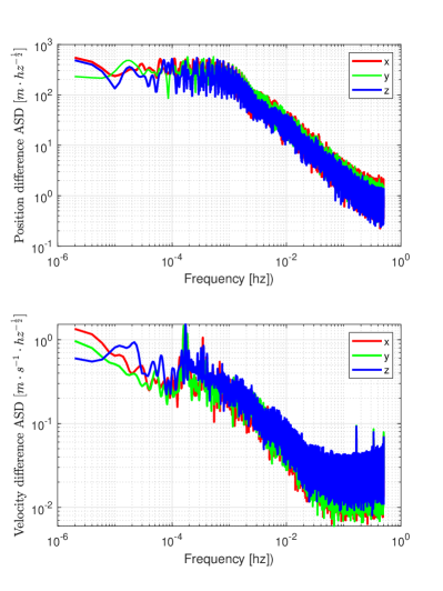
Figure 3: ASDs of the POD data differences between BD and GPS in the Earth-centered and Earth-fixed reference frame.

The S/C attitude is measured by star sensors, and the detailed information of how to rotate from the satellite frame to the inertial frame is provided by the Euler angle $\{\theta,\ \phi,\ \psi\}$ data product. In Fig. 4 the time series of the S/C attitude on 01-11-2019 are shown. The rotation matrices for each axis are given by

$$\mathbf{R}_{x}(\theta) = \left(\begin{matrix}1&0&0\\ 0&\cos\theta&\sin\theta\\ 0&-\sin\theta&\cos\theta\end{matrix}\right)$$ (6)

$$\mathbf{R}_{y}(\phi) = \left(\begin{matrix}\cos\phi&0&-\sin\phi\\ 0&1&0\\ \sin\phi&0&\cos\phi\end{matrix}\right)$$ (7)

$$\mathbf{R}_{z}(\psi) = \left(\begin{matrix}\cos\psi&\sin\psi&0\\ -\sin\psi&\cos\psi&0\\ 0&0&1\end{matrix}\right)$$ (8)

The total transformation matrix from the inertial reference frame to the satellite frame reads

$$\bm{R}=\bm{R}_{x}\bm{R}_{y}\bm{R}_{z}$$ (9)

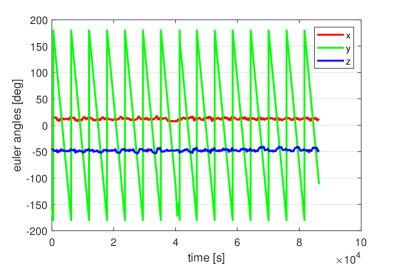
Figure 4: Time series of the S/C attitude data (Euler angles) on 01-11-2019.

The non-conservative forces are measured by the GRS in the accelerometer mode. The sensor unit of the electrostatic GRS on-board Taiji-1 contains two parts: the mechanical assembly and the front-end electronics unit. The mechanical assembly consists of a $72\ g$ parallel hexahedral titanium alloy test mass and an electrode cage that encloses the test mass. The test mass, as the inertial reference, is suspended electrostatically inside the cage. When non-gravitational forces acting on the S/C cause the relative motions between the test mass and the cage, the capacitance between the test mass and the electrodes changes slightly and induces signals that could be picked up by the front-end electronics unit. Based on the position sensor data, the test mass maintained its nominal position inside the cage by applying low frequency actuation voltages through the electrodes. The voltages sampled at 100 Hz are then transformed, with the calibrated bias and the scale factors, into the non-conservative accelerations exerted by the S/C in the satellite frame.

The sensitivities of the three GRS axes are different. The x-axis is pointing towards the Earth with low sensitivity, while the y-axis and z-axis are along the flight direction and the orbital normal direction respectively with high sensitivities. According to the in-orbit performance tests (The Taiji Scientific Collaboration, 2021; Min et al., 2021; Peng et al., 2021), the resolutions of the high sensitive axes reach the level of 1$0^{-10}$m/$s^{2}$/H$z^{1/2}$ in the frequency band from 0.01 Hz to 1 Hz and $10^{-9}m/s^{2}/Hz^{1/2}$ in the low frequency band from 0.1 mHz to 0.01 Hz. It will provide us the faithful measurements of the non-gravitational accelerations along Taiji-1’s orbit, according to the known force models. See Fig. 8 in the next section. Fig. 5 shows the ASDs of the measured non-gravitational accelerations in the satellite frame.

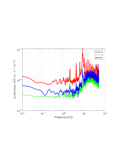
Figure 5: ASDs of the measured non-gravitational accelerations in the satellite frame.

III.2 Ancillary models

Table 1: Models for the perturbation forces

Perturbation	Model	Maximum degree
Earth’s gravity field	EGM2008	degree/order 100
Dealiasing	GRACE AOD1B RL06	degree/order 50
Ephemerides	JPL DE421
of Sun and Moon
Solid Earth tides	IERS2010	degree/order 4
Relativistic corrections	IERS2010
Atmospheric density	NRLMSISE-00
Earth Albedo	CERES

To determine the long wavelength and low-degree gravity field model, the interference from the high-degree geopotentials, the tidal signals and the 3rd-body perturbations needs to be suppressed or removed. In this work, the EGM2008 model (Pavlis et al., 2012) is employed as the prior gravity model, and also one of the reference models to assess and validate our Taiji-1 gravity model. Solid-Earth tides and the relativistic corrections are also considered according to the standard IERS2010 (Petit and Luzum, 2011). The 3rd-body perturbations from the Sun and the Moon are included, and the required position and the velocity vectors of the Sun and the Moon are obtained from JPL’s ephemerids DE421 (Folkner et al., 2009). The non-tidal atmospheric and oceanic mass variations are evaluated based on the atmosphere and ocean dealiasing product AOD1B RL06 (Dobslaw et al., 2017).

As mentioned, though fewer in the selected data, disruptions and gaps still exist, especially in the measurements of the GRS system. Therefore, the simulations of the non-gravitational forces calibrated and adjusted by the measurements along the orbits will be employed as the complementary data when the disturbances or the long term interruptions happen. In this work, the atmospheric density model NRLMSIS-00 (Picone et al., 2002) and Earth albedo model CERES (Wielicki et al., 1998, 2005) are used. The full list of all the models used can be found in Table 1.

IV Data processing

The software package TJGrav developed in this work for Taiji-1’s gravity field modeling contains three main sub-modules: the data Pre-Processor, the SST-Processor, and the Solver. Please see Fig. 6 for the architecture of TJGrav and the flow chart of the data processing procedure.

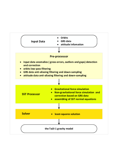
Figure 6: Software architecture of TJGrav and the flow chart of the data processing procedure.

Common manipulations including the data quality check, the identifications of gaps and gross errors, adding quality flags, the anomalies removing and replaced with interpolations, data smoothing, anti-aliasing and down-samplings are carried out by the Pre-processor.

Take the key POD data as an example. The quality of the data are generally good, but there are still gaps and outliers. The search for the data anomalies is executed in the first place. To make sure the continuity of the POD data in the observation equation 5, the outliers and the gaps are replaced or filled up with values evaluated by means of the Fourier least-square-fitting method. The replaced data will not be used to establish the normal equations, but only to calculate the integration in the observation equation 5. In the high frequency band of the POD data, the signal-to-noise ratio of the orbital perturbations from geopotentials decreases. Therefore, to suppress the high frequency noises, a low-pass filter at 0.005 Hz is imposed. After this, the POD data is down-sampled from 1 Hz to 0.2 Hz. The similar processing is applied to the original GRS data and S/C attitude data, and after a certain smoothing and anti-aliasing filtering they are also down-sampled to 0.2 Hz before use.

In the SST-Processor, we gather all the needed ancillary data, which are either obtained from the numerical simulations based on well-tested models or official data products released. Afterwards, the normal equation is established and ready to export to the Solver.

Required gravitational perturbations from other sources are modeled and calculated in the Earth-centered and Earth-fixed reference frame. As mentioned in the previous sections, the required data include perturbations from the 3rd-body (the Sun and the Moon), solid-Earth tides, AOD, and also the relativistic corrections. In the Earth-centered and Earth-fixed reference frame, the perturbation forces due to the 3rd-body is modeled as

$$\bm{a}_{\text{sun }}=-GM_{sun}\left(\frac{\bm{l}_{\text{sun }}}{\lvert\bm{l}_{\text{sun }}\rvert^{3}}+\frac{\bm{r}_{\text{sun }}}{\lvert\bm{r}_{\text{sun }}\rvert^{3}}\right)$$ (10)

$$\bm{a}_{\text{moon }}=-GM_{\text{moon }}\left(\frac{\bm{l}_{\text{moon }}}{\lvert\bm{l}_{\text{moon }}\rvert^{3}}+\frac{\bm{r}_{\text{moon }}}{\lvert\bm{r}_{\text{moon }}\rvert^{3}}\right)$$ (11)

where $M_{sun}$ and $M_{moon}$ are the masses of the Sun and the Moon, $\bm{l}_{\text{sun }}$, $\bm{l}_{\text{moon }}$ are the position vectors of the S/C relative to the Sun and the Moon, and $\bm{r}_{\text{sun }}$, $\bm{r}_{\text{moon }}$ the position vectors of the Earth relative to the Sun and the Moon. Please see Fig. 7 for the simulated gravitational perturbations on 01-11-2019.

Figure 7: Time series of the simulated gravitational perturbations in the earth-centered and earth-fixed reference frame on 01-11-2019.

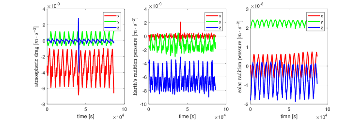
Figure 8: Time series of the simulated non-gravitational forces in the earth-centered and earth-fixed reference frame on 03-11-2019

The resolution power of the GRS on-board Taiji-1 ($\sim 10^{-10}m/s^{2}/Hz^{1/2}$) makes it sensible to small disturbances from the satellite platform. The test mass, as the inertial reference, couples to the surrounding physical fields in complicated ways. Events like temperature variations of the sensor unit, slight mechanical vibrations of the platforms and so on may cause the erroneous signals in the GRS measurements. The transient data anomalies of those kinds can be fixed by the Pre-Processor. However, continuous attitude adjustments with the reaction wheels, orbital maneuvers and certain experiments involving the GRS or the thrusters may cause the long term interruptions in the data. During the time, the modeled data of the non-gravitational forces are needed to fuse with the GRS measurements in order to fill the data-gaps.

As discussed in Sec. III, the air-drag is modeled as

$$\bm{a}_{drag}=-\frac{1}{2}\rho\frac{C_{D}A}{m_{SC}}\bm{v}_{rel}^{2}\frac{\bm{v}_{rel}}{\lvert\bm{v}_{rel}\rvert}$$ (12)

where $\rho$ is the air density, $C_{D}$ is the drag coefficient ($C_{D}=2.2$), $m_{SC}$ is the mass of the satellite, $\bm{v}_{rel}$ the velocity of the satellite relative to air, and $A$ is the windward area of the satellite. The radiation pressure either from the Solar radiation or the Earth albedo is modeled as

$$\bm{F}=\sum_{i}^{n}\bm{E}\frac{A_{i}\cos\theta}{c\,\,m_{SC}}\left[\left(1-\eta\right)\bm{\hat{E}}+2\eta\cos\theta\bm{\hat{n}}\right]$$ (13)

where $\bm{E}$ is the radiation flux, $A_{i}$ and $\bm{\hat{n}}$ denote the area and the normal direction of the S/C surface $i$, $\eta$ the fraction of the incoming radiation that is reflected by the surface $i$, and $\theta$ the angle between $\bm{E}$ and $\bm{\hat{n}}$. The key parameters in the above equations, the drag coefficient and the reflection coefficient, depend on the physical properties of the S/C surfaces and the real-time status of the surrounding environments, and may also change with time. Therefore, the modeled data is compared with the GRS measurements to adjust the parameters. In Fig. 8, we calibrate the simulated non-gravitational forces by the measured data from 01-11-2019. The magnitude of the simulated atmospheric drag is smaller than that of the Solar radiation pressure because of the 600 km altitude. In addition, one could also see that the averaged Solar radiation pressure along the pitch-axis (y-axis) of the satellite frame is the largest, since $\hat{\bm{y}}$ is the orbital normal direction oriented to the Sun.

Last but not the least, the high-degree geopotentials of degree/order from 21 to 100 along the Taiji-1’s orbit are derived from EGM2008. See Fig. 9 for the illustration.

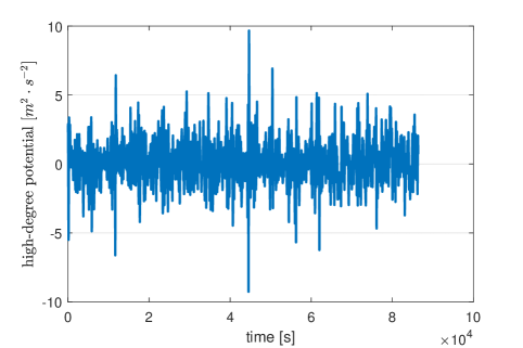
Figure 9: Time series of the high-degree geopotentials derived from EGM2008 for the spherical harmonic degree range 21 to 100 on 01-11-2019.(The greatest fluctuation around 44000 sec arises from transect across the Himalaya.)

Figure 10: Comparisons of the ASD curves of the observed geopotentials and those based on the EGM2008 model along the Taiji-1’s orbit.

Given all the processed measurement data and the modeled ancillary data so far, the observed low-degree Earth geopotentials along the orbit is solved by the SST-Processor based on the observation equation 5. In Fig. 10, the ASDs of the geopotentials along the orbit derived from both the BD and GPS measurements are compared with the simulated one based on the EGM2008 model. It is found that the geopotentials from the GPS agree quite well with the EGM2008 model for $f<$3.5 mHz. While, for frequency greater than 3.5 mHz, both of the BD and GPS results deviate significantly from the EGM2008 model. For Taiji-1’s orbit, the frequency of 3.5 mHz corresponds to about the 20th-degree spherical harmonics. This in fact indicates the precision limits of our gravity recovery method given the selected data sets. Therefore, the low-pass filter at 5 mHz is imposed on the POD data, and the signals from the high-degree geopotentials of degree/order from 21 to 100 are modeled and subtracted from the observations in advance to determine the low-degree gravity field up to degree/order 20.

Finally, in the Solver sub-modular, the normal equations based on Eq. 1 are constructed in the form

$$\bm{Ax}=\bm{b}$$ (14)

where $\bm{b}$ is the observation vector, $\bm{x}$ is consisted of the unknown geopotential coefficients, and $\bm{A}$ is the design matrix. The constrained gravity model is obtained in terms of the least-square solutions of the above normal equations with the first order Tikhonov regularization

$$\bm{x}=\left(\bm{A}^{\top}\bm{A}+\alpha\bm{K}\right)^{-1}\bm{A}^{\top}\bm{b}.$$ (15)

The elements $K_{ij}$ of the first order Tikhonov regularization matrix K read

$$K_{ij}=\delta_{ij}n(i)\left(n(i)+1\right),$$ (16)

where $n(i)$ is the degree $n$ of the element in the row $i$.

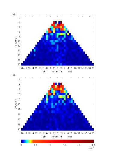
Figure 11: Geopotential coefficients of the Taiji-1’s gravity filed model TJGM-r1911 with the $C_{20}$ term removed: (a)BD; (b)GPS.

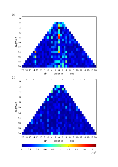
Figure 12: Differences between the Taiji-1 gravity model TJGM-r1911 and EGM2008: (a)BD; (b)GPS.

V Results

We have obtained the first monthly global gravity model from Taiji-1’s observations based on the measurements in November 2019. The geopotential data product, denoted as TJGM-r1911, is now archived by the Taiji-1 data processing center of CAS at Beijing, and it will be released soon together with the new monthly data products derived from the much better observations during Taiji-1’s extended free-falling phase in this year. These data products contain the geopotentials coefficients of spherical harmonics up to certain degree $\{C_{nm},\ S_{nm}\}$ and the corresponding variances $\{\Delta C_{mn},\ \Delta S_{nm}\}$.

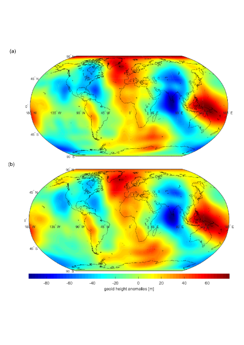
Figure 13: Geoid height anomalies of the Taiji-1 gravity model TJGM-r1911: (a)BD; (b)GPS.

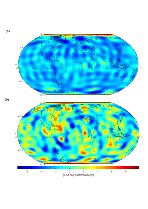
Figure 14: Geoid height differences between the Taiji-1 gravity model TJGM-r1911 and EGM2008: (a)BD; (b)GPS.

Figure 15: Degree RMS of the Taiji-1 gravity model error.

As mentioned previously, mainly because of the long term interruptions in the observation data, as well as the rather high orbit attitude of Taiji-1, our first product TJGM-r1911 is truncated at the 20th degree. To make the cross-check and comparisons, TJGM-r1911 also contains two independent sets of the geopotential data obtained from the GPS’s and BD’s observations respectively. Please see Fig. 11 and Fig. 13 for the comparisons. The differences from the reference models can be seen clearly in the plots in Fig. 12, Fig. 14 and Fig. 15. The gravity model from BD observations shows larger deviations from the reference models than that from the GPS observations. Also, in Fig. 15, the errors in terms of degree Root Mean Square is estimated from the prior reference model $\{C_{nm}^{P},\ S_{nm}^{P}\}$

$$RMS_{n}=\sqrt{\frac{\sum_{m=0}^{n}\left(C_{nm}-C_{nm}^{P}\right)^{2}+\sum_{m=1}^{n}\left(S_{nm}-S_{nm}^{P}\right)^{2}}{2n+1}},$$ (17)

the deviations of the TJGM-r1911 model from the reference models turns out to be larger than those from similar hl-SST missions. Compared with the gravity models from the CHAMP mission (Gerlach et al., 2003a, b; Weigelt et al., 2013; Foldvary et al., 2005; Mayer-Gurr et al., 2005; Han et al., 2002; Badura et al., 2006; Naeimi and Flury, 2017), the degree RMS of our TJGM-r1911 model is about one order of magnitude worse than that of the CHAMP models, depending on the used methods and ancillary data. The poor degree RMS comes from two factors. First, the Taiji-1’s orbit has a large inclination angle, and the altitude ($\sim 600$ km) is higher than all the gravity recovery satellites ever launched. Considering the key objectives of the Taiji-1 mission, this higher altitude was chosen to reduce the disturbances to the technology demonstration experiments from the space environment, especially the air drags. This inclination causes signals loss in the high latitude areas, and the higher altitude causes the magnitudes of the geopotentials at the orbit to decrease. Second, as already mentioned, the data is from the window period of the science operation phase, even though the data set is carefully selected, there still exist long interruptions and large disturbances, especially those for the key GRS measurements of the non-gravitational forces. The techniques such as data fusions with the calibrated simulations are employed to improve the fitting accuracy. However, the problem of the data quality and the discontinuity are believed to be the key reasons to the increased errors. Till the preparation of this work, the data from October 2019 to May 2020 and September 2020 to May 2021 had been analyzed. The missing months from June 2020 to August 2020 are due to the encounters of the satellite with the Earth’s shadow. During these months, because of the power supply issue, the key payloads including the GRS system were turned off to reduce risks. In the first few months until November 2019, instruments tests, calibrations and performance evaluations were still in progress, and in the following months much more experiments were scheduled. The precision of the geopotential product from October 2019 is comparable with that of TJGM-r1911, while the data from November 2019 is selected since it contains longer total operation time of the GRS system. For the subsequent months, the geopotential data qualities are rather worse. While, all these data discontinuities and anomalies will be greatly improved in the extended free-falling phase of Taiji-1 this year.

VI Conclusions and outlook

Gravity field is one of the fundamental physical fields of a planet. For Earth, the global gravity field contains vast amount of valuable information about the mass distributions and transfers on the Earth surface, the global climate changes, the groundwater storage, the Earth internal activities and so on. Great efforts have been paid in the satellite gravity, and after the CHAMP, GRACE, GOCE, and GRACE FO missions, the next generation gravity missions with advanced technologies including relativistic measurements are under investigations.

In this work, we carefully select the data of one month from Taiji-1’s observations, and develop the data fusion techniques to resolve the problem of the long term interruptions and the disturbances in the measurements caused by the scheduled technology demonstration experiments. The first global gravity model TJGM-r1911 independently derived from China’s own satellite mission is then successfully produced from the Taiji-1’s observations. The existed discrepancies between the first global gravity model TJGM-r1911 and the gravity models from CHAMP or other hl-SST missions are mainly caused by the data discontinuity problems. The capability of the Taiji-1 satellite serving as a fully-functional hl-SST satellite gravity mission for China has been demonstrated and confirmed. The extended free-falling phase of Taiji-1 with minimal disruptions and disturbances has been approved to be started this year. With the techniques developed in this work, Taiji-1 could serve as a satellite gravity mission for China, which could provide us independently both the static mappings of global gravity field and monthly averaged measurements of the time-variable gravity field.

Declarations

Conflict of Interest The authors have no competing interests to declare that are relevant to the content of this article.

References

- Danzmann (2011) K. Danzmann, Assessment Study Report, European Space Agency (2011).
- Bender (2004) P. L. Bender, Classical and Quantum Gravity 21, S1203 (2004), ISSN 0264-9381, 1361-6382, URL https://iopscience.iop.org/article/10.1088/0264-9381/21/5/120.
- Gong et al. (2011) X. Gong, S. Xu, S. Bai, Z. Cao, G. Chen, Y. Chen, X. He, G. Heinzel, Y.-K. Lau, C. Liu, et al., Classical and Quantum Gravity 28, 094012 (2011), ISSN 0264-9381, 1361-6382, URL https://iopscience.iop.org/article/10.1088/0264-9381/28/9/094012.
- Gong et al. (2015) X. Gong, Y.-K. Lau, S. Xu, P. Amaro-Seoane, S. Bai, X. Bian, Z. Cao, G. Chen, X. Chen, Y. Ding, et al., Journal of Physics: Conference Series 610, 012011 (2015), ISSN 1742-6588, 1742-6596, URL https://iopscience.iop.org/article/10.1088/1742-6596/610/1/012011.
- Xue-fei et al. (2015) G. Xue-fei, X. Sheng-nian, Y. Ye-fei, B. Shan, B. Xing, C. Zhou-jian, C. Ge-rui, D. Peng, G. Tian-shu, G. Wei, et al., Chinese Astronomy and Astrophysics 39, 411 (2015), ISSN 02751062, URL https://linkinghub.elsevier.com/retrieve/pii/S0275106215000843.
- The LIGO Scientific Collaboration et al. (2015) The LIGO Scientific Collaboration, J. Aasi, B. P. Abbott, R. Abbott, T. Abbott, M. R. Abernathy, K. Ackley, C. Adams, T. Adams, P. Addesso, et al., Classical and Quantum Gravity 32, 074001 (2015), ISSN 0264-9381, 1361-6382, URL https://iopscience.iop.org/article/10.1088/0264-9381/32/7/074001.
- Abbott et al. (2016a) B. P. Abbott, R. Abbott, T. D. Abbott, M. R. Abernathy, F. Acernese, K. Ackley, C. Adams, T. Adams, P. Addesso, R. X. Adhikari, et al., Physical Review Letters 116, 061102 (2016a), ISSN 0031-9007, 1079-7114, URL https://link.aps.org/doi/10.1103/PhysRevLett.116.061102.
- Abbott et al. (2016b) B. P. Abbott, R. Abbott, T. D. Abbott, M. R. Abernathy, F. Acernese, K. Ackley, C. Adams, T. Adams, P. Addesso, R. X. Adhikari, et al., Physical Review D 93, 122004 (2016b), ISSN 2470-0010, 2470-0029, URL https://link.aps.org/doi/10.1103/PhysRevD.93.122004.
- Abbott et al. (2016c) B. P. Abbott, R. Abbott, T. D. Abbott, M. R. Abernathy, F. Acernese, K. Ackley, C. Adams, T. Adams, P. Addesso, R. X. Adhikari, et al., Physical Review Letters 116, 241102 (2016c), ISSN 0031-9007, 1079-7114, URL https://link.aps.org/doi/10.1103/PhysRevLett.116.241102.
- Armano et al. (2016) M. Armano, H. Audley, G. Auger, J. T. Baird, M. Bassan, P. Binetruy, M. Born, D. Bortoluzzi, N. Brandt, M. Caleno, et al., Physical Review Letters 116, 231101 (2016), ISSN 0031-9007, 1079-7114, URL https://link.aps.org/doi/10.1103/PhysRevLett.116.231101.
- Armano et al. (2018) M. Armano, H. Audley, J. Baird, P. Binetruy, M. Born, D. Bortoluzzi, E. Castelli, A. Cavalleri, A. Cesarini, A. M. Cruise, et al., Physical Review Letters 120 (2018), ISSN 0031-9007, 1079-7114, URL https://link.aps.org/doi/10.1103/PhysRevLett.120.061101.
- Armano et al. (2019) M. Armano, H. Audley, J. Baird, P. Binetruy, M. Born, D. Bortoluzzi, E. Castelli, A. Cavalleri, A. Cesarini, A. M. Cruise, et al., Physical Review D 99, 082001 (2019), ISSN 2470-0010, 2470-0029, URL https://link.aps.org/doi/10.1103/PhysRevD.99.082001.
- Armano (2019) M. Armano, arXiv p. 1903.08924 (2019).
- Anderson et al. (2018) G. Anderson, J. Anderson, M. Anderson, G. Aveni, D. Bame, P. Barela, K. Blackman, A. Carmain, L. Chen, M. Cherng, et al., Physical Review D 98, 102005 (2018), ISSN 2470-0010, 2470-0029, URL https://link.aps.org/doi/10.1103/PhysRevD.98.102005.
- Cyranoski (2016) D. Cyranoski, Nature 531, 150 (2016), ISSN 0028-0836, 1476-4687, URL http://www.nature.com/articles/531150a.
- Hu and Wu (2017) W.-R. Hu and Y.-L. Wu, National Science Review 4, 685 (2017), ISSN 2095-5138, 2053-714X, URL http://academic.oup.com/nsr/article/4/5/685/4430188.
- Luo et al. (2020a) Z. Luo, Y. Wang, Y. Wu, W. Hu, and G. Jin, Progress of Theoretical and Experimental Physics p. ptaa083 (2020a), ISSN 2050-3911, URL https://academic.oup.com/ptep/advance-article/doi/10.1093/ptep/ptaa083/5875993.
- Luo et al. (2020b) Z. Luo, Z. Guo, G. Jin, Y. Wu, and W. Hu, Results in Physics 16, 102918 (2020b), ISSN 22113797, URL https://linkinghub.elsevier.com/retrieve/pii/S2211379719321928.
- Ruan et al. (2020a) W.-H. Ruan, Z.-K. Guo, R.-G. Cai, and Y.-Z. Zhang, International Journal of Modern Physics A 35, 2050075 (2020a), ISSN 0217-751X, 1793-656X, URL https://www.worldscientific.com/doi/abs/10.1142/S0217751X2050075X.
- The Taiji Scientific Collaboration et al. (2021) The Taiji Scientific Collaboration, Y.-L. Wu, Z.-R. Luo, J.-Y. Wang, M. Bai, W. Bian, H.-W. Cai, R.-G. Cai, Z.-M. Cai, J. Cao, et al., International Journal of Modern Physics A 36, 2102002 (2021), ISSN 0217-751X, 1793-656X, URL https://www.worldscientific.com/doi/abs/10.1142/S0217751X21020024.
- Ruan et al. (2020b) W.-H. Ruan, C. Liu, Z.-K. Guo, Y.-L. Wu, and R.-G. Cai, Nature Astronomy 4, 108 (2020b), ISSN 2397-3366, URL https://www.nature.com/articles/s41550-019-1008-4.
- Ruan et al. (2021) W.-H. Ruan, C. Liu, Z.-K. Guo, Y.-L. Wu, and R.-G. Cai, Research 2021, 1 (2021), ISSN 2639-5274, URL https://spj.sciencemag.org/journals/research/2021/6014164/.
- Wang et al. (2021a) R. Wang, W.-H. Ruan, Q. Yang, Z.-K. Guo, R.-G. Cai, and B. Hu, National Science Review p. nwab054 (2021a), ISSN 2095-5138, 2053-714X, URL https://academic.oup.com/nsr/advance-article/doi/10.1093/nsr/nwab054/6207944.
- Wang et al. (2021b) G. Wang, W.-T. Ni, W.-B. Han, P. Xu, and Z. Luo, Physical Review D 104, 024012 (2021b), ISSN 2470-0010, 2470-0029, URL https://link.aps.org/doi/10.1103/PhysRevD.104.024012.
- Liu et al. (2018a) H. Liu, Y. Dong, R. Gao, Z. Luo, and G. Jin, Optical Engineering 57, 1 (2018a), URL https://doi.org/10.1117/1.OE.57.5.054113.
- Liu et al. (2018b) H. Liu, Z. Luo, and G. Jin, Microgravity Sci. Technol. 30, 775 (2018b), URL https://doi.org/10.1007/s12217-018-9625-6.
- Li et al. (2018) Y. Li, Z. Luo, H. Liu, R. Gao, and G. Jin, Microgravity Sci. Technol. 30, 817 (2018), URL https://doi.org/10.1007/s12217-018-9624-7.
- Li et al. (2019) Y. Li, H. Liu, Y. Zhao, W. Sha, Z. Wang, Z. Luo, and G. Jin, Applied Sciences 9 (2019), ISSN 2076-3417, URL https://www.mdpi.com/2076-3417/9/10/2087.
- Li et al. (2020) Y. Li, C. Wang, L. Wang, H. Liu, and G. Jin, Microgravity Sci. Technol. 32, 331 (2020), URL https://doi.org/10.1007/s12217-019-09769-9.
- Liu et al. (2021) H. Liu, Y. Li, and G. Jin, Microgravity Sci. Technol. 33, 41 (2021), URL https://doi.org/10.1007/s12217-021-09875-7.
- The Taiji Scientific Collaboration (2021) The Taiji Scientific Collaboration, Communications Physics 4, 34 (2021), ISSN 2399-3650, URL http://www.nature.com/articles/s42005-021-00529-z.
- Moore et al. (2003) P. Moore, J. Turner, and Z. Qiang, Advances in Space Research 31, 1897 (2003), ISSN 02731177, URL https://linkinghub.elsevier.com/retrieve/pii/S0273117703001649.
- Naeimi and Flury (2017) M. Naeimi and J. Flury, eds., Global Gravity Field Modeling from Satellite-to-Satellite Tracking Data, Lecture Notes in Earth System Sciences (Springer International Publishing, Cham, 2017), ISBN 978-3-319-49940-6 978-3-319-49941-3, URL http://link.springer.com/10.1007/978-3-319-49941-3.
- Reigber (2005) C. Reigber, ed., Earth observation with CHAMP: results from three years in orbit (Springer, Berlin ; New York, 2005), ISBN 978-3-540-22804-2, meeting Name: CHAMP Science Meeting.
- O’Keefe (1957) J. A. O’Keefe, The Astronomical Journal 62, 265 (1957), ISSN 00046256, URL https://ui.adsabs.harvard.edu/abs/1957AJ.....62..265O/abstract.
- Hotine and Morrison (1969) M. Hotine and F. Morrison, Bulletin géodésique 91, 41 (1969), ISSN 0007-4632, URL http://link.springer.com/10.1007/BF02524844.
- Wolff (1969) M. Wolff, Journal of Geophysical Research 74, 5295 (1969), ISSN 01480227, URL http://doi.wiley.com/10.1029/JB074i022p05295.
- Jekeli (1999) C. Jekeli, Celestial Mechanics and Dynamical Astronomy 75, 85 (1999).
- Visser et al. (2003) P. N. A. M. Visser, N. Sneeuw, and C. Gerlach, Journal of Geodesy 77, 207 (2003), ISSN 0949-7714, 1432-1394, URL http://link.springer.com/10.1007/s00190-003-0315-8.
- Jacobi (1836) J. C. G. Jacobi, Monthly Reports of the Berlin Academy of Science July (1836).
- Gerlach et al. (2003a) C. Gerlach, N. Sneeuw, P. Visser, and D. Svehla, Advances in Geosciences 1, 73 (2003a), ISSN 1680-7359, URL https://adgeo.copernicus.org/articles/1/73/2003/.
- Gerlach et al. (2003b) C. Gerlach, L. Foldvary, D. Svehla, T. Gruber, M. Wermuth, N. Sneeuw, B. Frommknecht, H. Oberndorfer, T. Peters, M. Rothacher, et al., Geophysical Research Letters 30, 2003GL018025 (2003b), ISSN 0094-8276, 1944-8007, URL https://onlinelibrary.wiley.com/doi/abs/10.1029/2003GL018025.
- Foldvary et al. (2005) L. Foldvary, D. Svehla, C. Gerlach, M. Wermuth, T. Gruber, R. Rummel, M. Rothacher, B. Frommknecht, T. Peters, and P. Steigenberger, in Earth Observation with CHAMP, edited by C. Reigber, H. LÃŒhr, P. Schwintzer, and J. Wickert (Springer-Verlag, Berlin/Heidelberg, 2005), pp. 13–18, ISBN 978-3-540-22804-2, URL http://link.springer.com/10.1007/3-540-26800-6_2.
- Jaggi et al. (2011) A. Jaggi, H. Bock, L. Prange, U. Meyer, and G. Beutler, Advances in Space Research 47, 1020 (2011), ISSN 02731177, URL https://linkinghub.elsevier.com/retrieve/pii/S0273117710007350.
- Min et al. (2021) J. Min, J.-G. Lei, Y.-P. Li, D.-X. Xi, W.-Z. Tao, C.-H. Li, X.-Q. Zhang, Z.-L. Wang, D. Fan, Z.-R. Luo, et al., International Journal of Modern Physics A 36, 2140011 (2021), ISSN 0217-751X, 1793-656X, URL https://www.worldscientific.com/doi/abs/10.1142/S0217751X2140011X.
- Peng et al. (2021) X. Peng, H. Jin, P. Xu, Z. Wang, Z. Luo, X. Ma, L.-E. Qiang, W. Tang, X. Ma, Y. Zhang, et al., International Journal of Modern Physics A 36, 2140026 (2021), ISSN 0217-751X, 1793-656X, URL https://www.worldscientific.com/doi/abs/10.1142/S0217751X21400261.
- Pavlis et al. (2012) N. K. Pavlis, S. A. Holmes, S. C. Kenyon, and J. K. Factor, Journal of Geophysical Research: Solid Earth 117, n/a (2012), ISSN 01480227, URL http://doi.wiley.com/10.1029/2011JB008916.
- Petit and Luzum (2011) G. Petit and B. Luzum, IERS Technical Note No. 36, International Earth Rotation and Reference Systems Service (2011), URL https://apps.dtic.mil/sti/citations/ADA535671.
- Folkner et al. (2009) W. M. Folkner, J. G. Williams, and D. H. Boggs, The Interplanetary Network Progress Report vol. 42-178, p. 1-34 (2009).
- Dobslaw et al. (2017) H. Dobslaw, I. Bergmann-Wolf, R. Dill, L. Poropat, M. Thomas, C. Dahle, S. Esselborn, R. Konig, and F. Flechtner, Geophysical Journal International 211, 263 (2017), ISSN 0956-540X, 1365-246X, URL http://academic.oup.com/gji/article/211/1/263/3979461/A-new-highresolution-model-of-nontidal-atmosphere.
- Picone et al. (2002) J. M. Picone, A. E. Hedin, D. P. Drob, and A. C. Aikin, Journal of Geophysical Research: Space Physics 107, SIA 15 (2002), ISSN 01480227, URL http://doi.wiley.com/10.1029/2002JA009430.
- Wielicki et al. (1998) B. A. Wielicki, B. R. Barkstrom, B. A. Baum, T. P. Charlock, R. N. Green, D. P. Kratz, R. B. Lee, P. Minnis, G. L. Smith, T. Wong, et al., IEEE Transactions on Geoscience and Remote Sensing 36, 1127 (1998).
- Wielicki et al. (2005) B. A. Wielicki, T. Wong, N. Loeb, P. Minnis, K. Priestley, and R. Kandel, Science 308, 825 (2005).
- Weigelt et al. (2013) M. Weigelt, T. Dam, A. Jaggi, L. Prange, M. J. Tourian, W. Keller, and N. Sneeuw, Journal of Geophysical Research: Solid Earth 118, 3848 (2013), ISSN 2169-9313, 2169-9356, URL https://onlinelibrary.wiley.com/doi/10.1002/jgrb.50283.
- Mayer-Gurr et al. (2005) T. Mayer-Gurr, K. Ilk, A. Eicker, and M. Feuchtinger, Journal of Geodesy 78, 462 (2005), ISSN 0949-7714, 1432-1394, URL http://link.springer.com/10.1007/s00190-004-0413-2.
- Han et al. (2002) S.-C. Han, C. Jekeli, and C. K. Shum, Geophysical Research Letters 29, 36 (2002), ISSN 00948276, URL http://doi.wiley.com/10.1029/2002GL015180.
- Badura et al. (2006) T. Badura, C. Sakulin, C. Gruber, and R. Klostius, Studia Geophysica et Geodaetica 50, 59 (2006), ISSN 0039-3169, 1573-1626, URL http://link.springer.com/10.1007/s11200-006-0002-3.