A well-balanced scheme for Euler equations with singular sources

Abstract

Numerical methods for the Euler equations with a singular source are discussed in this paper. The stationary discontinuity induced by the singular source and its coupling with the convection of fluid presents challenges to numerical methods. We show that the splitting scheme is not well-balanced and leads to incorrect results; in addition, some popular well-balanced schemes also give incorrect solutions in extreme cases due to the singularity of source. To fix such difficulties, we propose a solution-structure based approximate Riemann solver, in which the structure of Riemann solution is first predicted and then its corresponding approximate solver is given. The proposed solver can be applied to the calculation of numerical fluxes in a general finite volume method, which can lead to a new well-balanced scheme. Numerical tests show that the discontinuous Galerkin method based on the present approximate Riemann solver has the ability to capture each wave accurately.

Keywords: hyperbolic conservation law, Euler equation, Riemann problem, singular source, Riemann solver, well-balanced scheme

AMS subject classifications: 35L867,35Q31,65M60,76N30

1 Introduction

The governing equations for many mechanical problems involving fluids are hyperbolic conservation laws with singular sources. For example, surface tension [18, 26], evaporation[15, 16, 17], phase transition[25, 32, 33, 40, 42, 43] and condensation[11] at the interface of multiphase flows are formulated by singular sources. Geometric constraints on irregular domains can also lead to the generation of singular sources in simplified governing equations, such as the shallow water equations with discontinuous river beds[19, 35, 39] and the governing equations of nozzle flow with discontinuous cross-section[13, 44]. In addition, the damping term in the fluid under consideration behaves as a singular source when it is smaller than the grid size[21].

In this paper we consider the Euler equations with a singular source:

$$\partial_{t}U+\partial_{x}F(U)=\delta(x)S,$$ (1.1)

where

$$U=\begin{pmatrix}\rho\\ \rho u\\ E\end{pmatrix},F=\begin{pmatrix}\rho u\\ \rho u^{2}+p\\ (E+p)u\end{pmatrix},\delta(x)=\begin{cases}0,\ x\neq 0\\ \infty,\ x=0\end{cases}$$

Here, $\rho$, $p$ and $E$ denote the density, pressure and total energy, respectively. $u$ is the velocity. $S$ is the vector of souce term distributed only at the origin. Let $U_{-}=U(0-,t)$ and $U_{+}=U(0+,t)$ denote the states to the left-hand and right-hand sides of the origin, respectively, and the source leads to $U_{-}\neq U_{+}$. The source term in this paper is a generalisation of the source term in [11]:

$$S(U_{-},U_{+})=\begin{cases}S(F(U_{-}))=diag(k_{1},k_{2},k_{3})F(U_{-}),\ \text{if}\ u_{-}>0,u_{+}>0\\ S(F(U_{+}))=diag(k_{1},k_{2},k_{3})F(U_{+}),\ \text{if}\ u_{-}<0,u_{+}<0\\ 0,\ else\\ \end{cases}$$ (1.2)

where $diag(k_{1},k_{2},k_{3})$ is the diagonal matrix with constant diagonal element $k_{1}>-1$, $k_{2}>-1$ and $k_{3}>-1$. This paper deals only with the ideal gas, whose equation of state is

$$RT=p/\rho,\ p=(\gamma-1)\rho e,\ \gamma>1,$$

where $\gamma$ is the ratio of specific heats, $e$ is the internal energy, $T$ is the temperature and $R$ is the universal gas constant.

The aim of this paper is to develop a numerical method for hyperbolic conservation laws with singular sources, which is capable of giving numerical solutions in good agreement with the exact solution.

The most commonly used schemes are basesd on splitting techniques, which solves iteratively the partial differential equation associated to the convection and the ordinary differential equation associated to the source (see [4, 47]). Unfortunately, the numerical solution obtained by such a simple method is inaccurate, even if the source term is discretized by a upwind manner. Small errors in the approximate solution near the singular source may become uncontrolled under the splitting scheme, and this error does not decrease as the grid size decreases, see [2, 5, 30, 31, 36]. One reason for such error is that the splitting scheme is not well-balanced (also known as C-property, see [1, 23, 39, 4]), which refers to the ability of the numerical scheme to maintain precisely the equilibrium state near singular source or some steady solutions. Many scholars have been working on the development of well-balanced schemes, such as [1, 2, 5, 7, 6, 9, 8, 36, 47, 31, 46, 20, 29, 38, 37, 3, 41, 27, 28, 48]. Among those schemes, we focus on the well-balanced scheme proposed by Kröner and Thanh in [31] and referred to in this paper as the K-T scheme to distinguish it from the well-balanced preperty. One advantage of K-T scheme is that it can be directly generalised to arbitrary equations as long as the solution to the discontinuity induced by singular sources can be obtained explicitly. We apply K-T scheme to equation (1.1) and obtained good results in the non-extreme case. In some extreme cases, referred to as choked solutions in this paper, the results of K-T scheme are not satisfactory. Similar errors of K-T scheme have been reported in [45].

The Godunov scheme, which constructs the numerical flux by the exact Riemann solution, is well-balanced for hyperbolic conservation laws with singular sources(see [14, 24, 35, 36]). However, the complete Riemann solution of (1.1) is generally not available. In this paper we apply the approximate Riemann solver to construct the numerical flux at singular sources. In order for the numerical scheme to be well-balanced, the approximate Riemann solver must give an exact solution when the initial value is a single stationary wave. Based on our previous analysis of the Riemann problem in [50], we propose a structure-based approximate Riemann solver. The proposed solver not only ensures the well-balanced property of the numerical scheme, but also is effective in extreme cases due to the coupled treatment of sources and convection. In this paper the numerical scheme of combining the proposed Riemann solver with a discontinuous Galerkin method gives satisfactory numerical solutions in both extreme and non-extreme cases.

This paper is organized as follows. Section2 is about preliminaries to the Riemann solution. InSection 3, we will present splitting methods and unsplitting methods, and their performance for the well-balanced property. In Section4 we will be concerned with the numerical flux for singular sources. We will first discuss the numerical flux of the K-T scheme and then present an approximate Riemann solver and the numerical flux based on the solver. The results of the splitting scheme, the K-T scheme and the present solver-based scheme in conjunction with the discontinuous Galerkin method for solving a steady solution and seven Riemann solutions of different structures, respectively, will be put in Section5. Finally, some conclusions will be given in Section6.

2 Preliminaries

In this section we list some conclusions on the following Riemann problems:

$$\begin{cases}\partial_{t}U+\partial_{x}F(U)=\delta(x)S\\ U(x,0)=\begin{cases}U_{L},\ x<0\\ U_{R},\ x>0\end{cases}\end{cases}$$ (2.1)

First of all, we give the definition of the stationary wave induced by the singular source in Section2.1. Then, we give a brief overview of all the elementary waves of the Riemann problem of the classical Euler equations in Section2.2. Finally, we give all possible structures of Riemann solution in Section2.3. For the related proofs, readers are referred to [50].

2.1 Stationary wave

The stationary wave is a discontinuity in the Riemann solution that lies constantly on the t-axis. We denote the left-hand and right-hand states of a stationary wave as $U_{-}$ and $U_{+}$, respectively. Let $u_{-}$ and $u_{+}$ denote the velocity of $U_{-}$ and $U_{+}$ respectively, then $u_{-}$ and $u_{+}$ have the same sign. In this section we assume $u_{-}>0$ and $u_{+}>0$. $U_{-}$ and $U_{+}$ satisfy the jump relation:

$$F(U_{-})+S(F(U_{-}))=F(U_{+}),$$ (2.2)

therefore the stationary wave is a local steady solution. $U_{-}$ and $U_{+}$ are called equilibrium states.

For a given $U_{-}$, there are two branches of $U_{+}$ that satisfy (2.2) with $k_{1},k_{2},k_{3}$ as parameters, which are referred to as subsonic branch and supersonic branch, respectively. In order to select physical equilibrium states, we employ the following criterion proposed in [50]:

Monotonicity Criterion 1

Given coefficients $k_{1}$, $k_{2}$ and $k_{3}$, the left-hand state $U_{-}$ and right-hand state $U_{+}$ of a stationary wave satisfies $\lambda_{k}(U_{-})\cdot\lambda_{k}(U_{+})\geq 0,\forall 1\leq k\leq 3$.

Let $M_{-}$ and $M_{+}$ denote the Mach numbers of $U_{-}$ and $U_{+}$, respectively. The admissible sets of $M_{-}$ and $M_{+}$ are denoted as $\Gamma_{-}$ and $\Gamma_{+}$, respectively. Within the restriction of Criterion1, $\Gamma_{-}$ and $\Gamma_{+}$ are shown in Table1.

Table 1: The admissible sets of $M_{-}$ and $M_{+}$.

$k$	subsonic branch		supersonic branch
	$\Gamma_{-}$	$\Gamma_{+}$	$\Gamma_{-}$	$\Gamma_{+}$
$(0,+\infty)$	$(0,M_{1}^{*}]$	$(0,1]$	$\left[M^{*}_{2},+\infty\right)$	$\left[1,M_{3}^{*}\right)$
${0}$	$(0,1]$	$(0,1]$	$\left[1,+\infty\right)$	$\left[1,+\infty\right)$
$(-\infty,0)$	$(0,1]$	$(0,M_{1}^{**}]$	$\left[1,M_{3}^{**}\right)$	$\left[M_{2}^{**},+\infty\right)$

The definitions of the symbols in Table1 are given below.

$$k=(1+k_{1})(1+k_{3})/(1+k_{2})^{2}-1.$$ (2.3)

$$M_{1}^{*}=\begin{cases}\sqrt{\frac{k\gamma+k+1-(\gamma+1)\sqrt{k(k+1)}}{k+1-k\gamma^{2}}},\ &\text{if}\ k\neq\frac{1}{\gamma^{2}-1},\ k>0\\ \sqrt{\frac{\gamma-1}{2\gamma}},\ &\text{if}\ k=\frac{1}{\gamma^{2}-1}\end{cases}$$ (2.4)

$$M_{2}^{*}=\begin{cases}\sqrt{\frac{k\gamma+k+1+(\gamma+1)\sqrt{k(k+1)}}{k+1-k\gamma^{2}}},\ &\text{if}\ 0<k<\frac{1}{\gamma^{2}-1}\\ +\infty,\ &\text{if}\ k\geq\frac{1}{\gamma^{2}-1}\end{cases}$$

$$M_{3}^{*}=\begin{cases}\sqrt{\frac{\gamma+\sqrt{1-k(\gamma^{2}-1)}}{\gamma-\gamma\sqrt{1-k(\gamma^{2}-1)}}},\ &\text{if}\ 0<k<\frac{1}{\gamma^{2}-1}\\ +\infty,\ &\text{if}\ k\geq\frac{1}{\gamma^{2}-1}\end{cases}$$

$$M_{1}^{**}=\sqrt{\frac{1-\sqrt{-k}}{1+\gamma\sqrt{-k}}},\ \text{if}\ k<0$$ (2.5)

$$M_{2}^{**}=\begin{cases}\sqrt{\frac{1+\sqrt{-k}}{1-\gamma\sqrt{-k}}},\ &\text{if}\ -\frac{1}{\gamma^{2}}<k<0\\ +\infty,\ &\text{if}\ -1<k\leq-\frac{1}{\gamma^{2}}\end{cases}$$

$$M_{3}^{**}=\begin{cases}\sqrt{\frac{\gamma\sqrt{1+k}+\sqrt{1+k\gamma^{2}}}{\gamma\sqrt{1+k}-\gamma\sqrt{1+k\gamma^{2}}}},\ &\text{if}\ -\frac{1}{\gamma^{2}}<k<0\\ 1,\ &\text{if}\ -1<k\leq-\frac{1}{\gamma^{2}}\end{cases}$$

Given a left-hand state $U_{-}$ of the stationary wave, the wave curve $\mathcal{D}(U_{-},k_{1},k_{2},k_{3})$ denotes all right-hand states $U_{+}$ that can be connected to $U_{-}$ by the stationary wave with coefficients $k_{1},k_{2},k_{3}$. Given a right-hand state $U_{+}$ of the stationary wave, the wave curve $\mathcal{D}^{B}(U_{+},k_{1},k_{2},k_{3})$ denotes all left-hand states $U_{-}$ that can be connected to $U_{+}$ by the stationary wave with coefficients $k_{1},k_{2},k_{3}$.

Under Criterion1, the wave curve of the stationary wave has following properties without proof. For details, readers are referred to [50].

$$\mathcal{D}(U_{-},k_{1},k_{2},k_{3}):$$ (2.6)

$$\begin{aligned} &\rho_{+}=\rho_{-}\left(\frac{M_{-}}{M_{+}}\right)^{2}\frac{\gamma M_{+}^{2}+1}{\gamma M_{-}^{2}+1}\frac{(1+k_{1})^{2}}{1+k_{2}},\\ &u_{+}=u_{-}\left(\frac{M_{+}}{M_{-}}\right)^{2}\frac{\gamma M_{-}^{2}+1}{\gamma M_{+}^{2}+1}\frac{1+k_{2}}{1+k_{1}},\\ &p_{+}=p_{-}\frac{\gamma M_{-}^{2}+1}{\gamma M_{+}^{2}+1}(1+k_{2}),\end{aligned}\left\{\begin{aligned} &\text{if}\ k>0,\ M_{+}=\begin{cases}\sqrt{\frac{1-I}{1+\gamma I}},\ 0<M_{-}\leq M_{1}^{*}\\ \sqrt{\frac{1+I}{1-\gamma I}},\ M_{2}^{*}\leq M_{-}<+\infty\end{cases}\\ &\text{if}\ k<0,\ M_{+}=\begin{cases}\sqrt{\frac{1-I}{1+\gamma I}},\ 0<M_{-}\leq 1\\ \sqrt{\frac{1+I}{1-\gamma I}},\ 1\leq M_{-}<M_{3}^{**}\\ \end{cases}\\ &\text{if}\ k=0,\ M_{+}=\begin{cases}\sqrt{\frac{1-I}{1+\gamma I}},\ 0<M_{-}\leq 1\\ \sqrt{\frac{1+I}{1-\gamma I}},\ 1<M_{-}<+\infty\\ \end{cases}\\ \end{aligned}\right.$$

Here,

$$I=\frac{\sqrt{(\gamma M_{-}^{2}+1)^{2}-(\gamma+1)M_{-}^{2}[(\gamma-1)M_{-}^{2}+2](1+k)}}{\gamma M_{-}^{2}+1},$$

$$\mathcal{D}^{B}(U_{+},k_{1},k_{2},k_{3}):$$ (2.7)

$$\begin{aligned} &\rho_{-}=\rho_{+}\left(\frac{M_{+}}{M_{-}}\right)^{2}\frac{\gamma M_{-}^{2}+1}{\gamma M_{+}^{2}+1}\frac{1+k_{2}}{(1+k_{1})^{2}},\\ &u_{-}=u_{+}\left(\frac{M_{-}}{M_{+}}\right)^{2}\frac{\gamma M_{+}^{2}+1}{\gamma M_{-}^{2}+1}\frac{1+k_{1}}{1+k_{2}},\\ &p_{-}=p_{+}\frac{\gamma M_{+}^{2}+1}{\gamma M_{-}^{2}+1}\frac{1}{1+k_{2}},\end{aligned}\left\{\begin{aligned} &\text{if}\ k>0,\ M_{-}=\begin{cases}\sqrt{\frac{1-I^{B}}{1+\gamma I^{B}}},\ 0<M_{+}\leq 1\\ \sqrt{\frac{1+I^{B}}{1-\gamma I^{B}}},\ 1\leq M_{+}<M^{*}_{3}\\ \end{cases}\\ &\text{if}\ k<0,\ M_{-}=\begin{cases}\sqrt{\frac{1-I^{B}}{1+\gamma I^{B}}},\ 0<M_{+}\leq M^{**}_{1}\\ \sqrt{\frac{1+I^{B}}{1-\gamma I^{B}}},\ M^{**}_{2}\leq M_{+}<+\infty\end{cases}\\ &\text{if}\ k=0,\ M_{-}=\begin{cases}\sqrt{\frac{1-I^{B}}{1+\gamma I^{B}}},\ 0<M_{-}\leq 1\\ \sqrt{\frac{1+I^{B}}{1-\gamma I^{B}}},\ 1<M_{-}<+\infty\\ \end{cases}\\ \end{aligned}\right.$$

Here,

$$I^{B}=\frac{\sqrt{(\gamma M_{+}^{2}+1)^{2}-(\gamma+1)M_{+}^{2}[(\gamma-1)M_{+}^{2}+2]/(1+k)}}{\gamma M_{+}^{2}+1},$$

Property 2.1

For the stationary wave with given left-hand state $U_{-}$ and coefficients $k_{1},k_{2},k_{3}$,

• $D(U_{-},k_{1},k_{2},k_{3})$ is a singleton set iff

  $$k>0\ \&\ M_{1}^{*}<M_{-}<M_{2}^{*}\quad\text{or}\quad k<0\ \&\ M_{-}\geq M_{3}^{**};$$

• $D(U_{-},k_{1},k_{2},k_{3})$ is a set of two elements iff $k<0\ \&\ M_{-}=1$;

• $D(U_{-},k_{1},k_{2},k_{3})=\emptyset$ in other cases.

An extreme case of the stationary wave is known as the choke, which is defined as

Definition 2.1

A stationary wave is said to be choked if its left-hand state $U_{-}$ and right-hand state $U_{+}$ satisfy $\exists 1\leq k\leq m,s.t.\ \lambda_{k}(U_{-})\cdot\lambda_{k}(U_{+})=0$.

A Riemann solution is said to be choked if it contains a choked stationary wave.

By (2.6) and (2.7), the strength of the stationary wave is determined by $M_{-}$. For the convenience of following discussion, we use some notations to represent the solution of stationary wave:

$$M_{+}=g_{M}^{\mathcal{D}}(M_{-}),\ \frac{\rho_{+}}{\rho_{-}}=g_{d}^{\mathcal{D}}(M_{-}),\ \frac{u_{+}}{u_{-}}=g_{u}^{\mathcal{D}}(M_{-}),\ \frac{p_{+}}{p_{-}}=g_{p}^{\mathcal{D}}(M_{-}).$$

When $k<0\&M_{-}=1$, the functions $g_{M}^{\mathcal{D}}$, $g_{d}^{\mathcal{D}}$, $g_{u}^{\mathcal{D}}$, $g_{p}^{\mathcal{D}}$ are all double-valued, where one is supersonic and the other is subsonic. We need to specify which branch to use in this case.

2.2 Shock waves, rarefaction waves and contact discontinuities

There are three elementary waves in the Riemann problem for the classical Euler equations, namely Lax shock waves, rarefaction waves and contact discontinuities. We define some functions to represent the relations between the left-hand and right-hand states of these three elementary waves, and for a detailed introduction readers are referred to [47, 10].

The characteristic domains of $\lambda_{1}$ and $\lambda_{3}$ are both genuinely nonlinear. The elementary wave associated with these two characteristic domains is either a shock wave or a rarefaction wave. We denote

$$f_{d}^{1-\mathcal{S}}(U_{0},p)\mathop{=}\limits^{def}\rho_{0}\frac{(\gamma-1)p_{0}+(\gamma+1)p}{(\gamma-1)p+(\gamma+1)p_{0}},\ p\geq p_{0}$$ (2.8)

$$f_{u}^{1-\mathcal{S}}(U_{0},p)\mathop{=}\limits^{def}u_{0}-\sqrt{2}(p-p_{0})/\sqrt{\rho_{0}((\gamma+1)p+(\gamma-1)p_{0})},\ p\geq p_{0}$$

$$f_{M}^{1-\mathcal{S}}(U_{0},p)\mathop{=}\limits^{def}f_{u}^{1-\mathcal{S}}(U_{0},p)\sqrt{f_{d}^{1-\mathcal{S}}(U_{0},p)}/\sqrt{\gamma p},\ p\geq p_{0}$$

$$f_{d}^{3-\mathcal{S}}(U_{0},p)\mathop{=}\limits^{def}\rho_{0}\frac{(\gamma-1)p_{0}+(\gamma+1)p}{(\gamma-1)p+(\gamma+1)p_{0}},\ p\geq p_{0}$$

$$f_{u}^{3-\mathcal{S}}(U_{0},p)\mathop{=}\limits^{def}u_{0}+\sqrt{2}(p-p_{0})/\sqrt{\rho_{0}((\gamma+1)p+(\gamma-1)p_{0})},\ p\geq p_{0}$$

$$f_{M}^{3-\mathcal{S}}(U_{0},p)\mathop{=}\limits^{def}f_{u}^{3-\mathcal{S}}(U_{0},p)\sqrt{f_{d}^{3-\mathcal{S}}(U_{0},p)}/\sqrt{\gamma p},\ p\geq p_{0}$$

Given the left-hand state $U_{0}$ of a $\lambda_{1}-$shock wave, the right-hand state with the pressure $p$ satisfies

$$\rho=f_{d}^{1-\mathcal{S}}(U_{0},p),u=f_{u}^{1-\mathcal{S}}(U_{0},p),M=f_{M}^{1-\mathcal{S}}(U_{0},p).$$

Given the right-hand state $U_{0}$ of a $\lambda_{3}-$shock wave, the left-hand state with the pressure $p$ satisfies

$$\rho=f_{d}^{3-\mathcal{S}}(U_{0},p),u=f_{u}^{3-\mathcal{S}}(U_{0},p),M=f_{M}^{3-\mathcal{S}}(U_{0},p).$$

Let

$$f_{d}^{1-\mathcal{R}}(U_{0},p)\mathop{=}\limits^{def}\rho_{0}\left(p/p_{0}\right)^{\frac{1}{\gamma}},\ p\leq p_{0}$$ (2.9)

$$f_{u}^{1-\mathcal{R}}(U_{0},p)\mathop{=}\limits^{def}u_{0}-2a_{0}/(\gamma-1)\left[\left(p/p_{0}\right)^{\frac{\gamma-1}{2\gamma}}-1\right],\ p\leq p_{0}$$

$$f_{d}^{3-\mathcal{R}}(U_{0},p)\mathop{=}\limits^{def}\rho_{0}\left(p/p_{0}\right)^{\frac{1}{\gamma}},\ p\leq p_{0}$$

$$f_{u}^{3-\mathcal{R}}(U_{0},p)\mathop{=}\limits^{def}u_{0}+2a_{0}/(\gamma-1)\left[\left(p/p_{0}\right)^{\frac{\gamma-1}{2\gamma}}-1\right],\ p\leq p_{0}$$

Given the left-hand state $U_{0}$ of a $\lambda_{1}-$rarefaction wave, the right-hand state with the pressure $p$ satisfies

$$\rho=f_{d}^{1-\mathcal{S}}(U_{0},p),u=f_{u}^{1-\mathcal{S}}(U_{0},p).$$

Given the right-hand state $U_{0}$ of a $\lambda_{3}-$rarefaction wave, the left-hand state with the pressure $p$ satisfies

$$\rho=f_{d}^{3-\mathcal{S}}(U_{0},p),u=f_{u}^{3-\mathcal{S}}(U_{0},p).$$

We denote

$$g_{d}^{1-\mathcal{R}}(M_{0},M)\mathop{=}\limits^{def}g_{d}^{3-\mathcal{R}}(M_{0},M)\mathop{=}\limits^{def}\left[\frac{(\gamma-1)M_{0}+2}{(\gamma-1)M+2}\right]^{\frac{2}{\gamma-1}},\ M\geq M_{0}.$$ (2.10)

$$g_{u}^{1-\mathcal{R}}(M_{0},M)\mathop{=}\limits^{def}g_{u}^{3-\mathcal{R}}(M_{0},M)\mathop{=}\limits^{def}\frac{M}{M_{0}}\left[\frac{(\gamma-1)M_{0}+2}{(\gamma-1)M+2}\right],\ M\geq M_{0}.$$

$$g_{p}^{1-\mathcal{R}}(M_{0},M)\mathop{=}\limits^{def}g_{p}^{3-\mathcal{R}}(M_{0},M)\mathop{=}\limits^{def}\left[\frac{(\gamma-1)M_{0}+2}{(\gamma-1)M+2}\right]^{\frac{2\gamma}{\gamma-1}},\ M\geq M_{0}.$$

Given the left-hand state $U_{0}$ of a $\lambda_{1}-$rarefaction wave, the right-hand state with the Mach number $M$ satisfies

$$\rho=\rho_{0}g_{d}^{1-\mathcal{R}}(M_{0},M),u=u_{0}g_{u}^{1-\mathcal{R}}(M_{0},M),p=p_{0}g_{p}^{1-\mathcal{R}}(M_{0},M).$$

Given the right-hand state $U_{0}$ of a $\lambda_{3}-$rarefaction wave, the left-hand state with the Mach number $M$ satisfies

$$\rho=\rho_{0}g_{d}^{3-\mathcal{R}}(M_{0},M),u=u_{0}g_{u}^{3-\mathcal{R}}(M_{0},M),p=p_{0}g_{p}^{3-\mathcal{R}}(M_{0},M).$$

The characteristic domain of $\lambda_{2}=u$ is linearly degenerate. The elementary wave associated with the $\lambda_{2}$ characteristic domain is the contact discontinuity.

In summary, we have

$$f_{d}^{1-\mathcal{W}}(U_{0},p)=\begin{cases}f_{d}^{1-\mathcal{S}}(U_{0},p),\ p\geq p_{0}\\ f_{d}^{1-\mathcal{R}}(U_{0},p),\ p<p_{0}\end{cases}f_{u}^{1-\mathcal{W}}(U_{0},p)=\begin{cases}f_{u}^{1-\mathcal{S}}(U_{0},p),\ p\geq p_{0}\\ f_{u}^{1-\mathcal{R}}(U_{0},p),\ p<p_{0}\end{cases}$$

$$f_{d}^{3-\mathcal{W}}(U_{0},p)=\begin{cases}f_{d}^{3-\mathcal{S}}(U_{0},p),\ p\leq p_{0}\\ f_{d}^{3-\mathcal{R}}(U_{0},p),\ p>p_{0}\end{cases}f_{u}^{3-\mathcal{W}}(U_{0},p)=\begin{cases}f_{u}^{3-\mathcal{S}}(U_{0},p),\ p\leq p_{0}\\ f_{u}^{3-\mathcal{R}}(U_{0},p),\ p>p_{0}\end{cases}$$

2.3 Riemann problem

This section presents the structure of the solution to the Riemann problem (2.1). We first consider its associate Riemann problem, that is, the following classical Riemann problem for the Euler equations:

$$\left\{\begin{aligned} &\frac{\partial U}{\partial t}+\frac{\partial F}{\partial x}=0,\\ &U(x,0)=\begin{cases}U_{L},\ x<0\\ U_{R},\ x>0\end{cases}\end{aligned}\right.$$ (2.11)

The solution of the associative Riemann problem (2.11) is self-similar and contains four constant regions, which are divided by three classical elementary waves, as shown in the left figure of Figure1. Although the governing equation (1.1) contains source terms, it is clearly still self-similar, we therefore assume that the solution to the Riemann problem (2.1) is self-similar.

The self-similar solution of Riemann problem (2.1) and associate Riemann problem (2.11) with the initial value condition $U_{L}$ and $U_{R}$ are denoted as $U^{R}\left(\frac{x}{t},U_{L},U_{R}\right),\ U^{A-R}\left(\frac{x}{t},U_{L},U_{R}\right)$, respectively. We have following conclusions as shown in [50].

Proposition 2.1 (Double CRP framework)

The self-similar solution of the Riemann problem consists of seven discontinuities at most. They are a stationary wave at $x=0$, two genuinely nonlinear waves and a contact discontinuity left to $x=0$, two genuinely nonlinear waves and a contact discontinuity right to $x=0$ respectively.

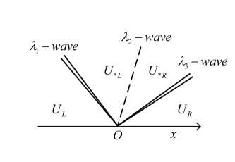
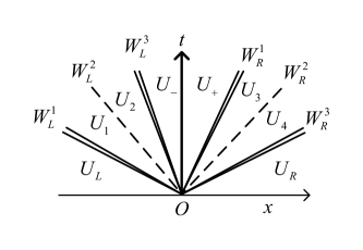
Figure 1: The general structure of Riemann solutions. Left: associate Riemann problem (2.1). Right: Riemann problem (2.11).

According to Proposition2.1, the general structure of Riemann solutions is shown in the right figure of Figure1. The elementary waves on the left and right sides are denoted as $W_{L}^{1}$, $W_{L}^{2}$, $W_{L}^{3}$ and $W_{R}^{1}$, $W_{R}^{2}$, $W_{R}^{3}$, respectively. $W_{L}^{1}$, $W_{L}^{3}$, $W_{R}^{1}$ and $W_{R}^{3}$ can be shock waves or rarefaction waves, and both $W_{L}^{2}$ and $W_{R}^{2}$ are contact discontinuities. The t-axis is a stationary wave and $U_{-}\neq U_{+}$. We follow the notation of [34, 44] to express the structure of Riemann solutions. For example, $\mathcal{S}(U_{L},U_{1})$ and $\mathcal{R}(U_{L},U_{1})$ mean that two states $U_{L}$ and $U_{1}$ are connected by a shock and a rarefaction wave, respectively. The symbol $\mathcal{W}(U_{L},U_{1})$ means that $U_{L}$ and $U_{1}$ are connected by a shock wave or a rarefaction wave. $\mathcal{C}(U_{1},U_{2})$ means that $U_{1}$ and $U_{2}$ are connected by a contact discontinuity, and $\mathcal{D}(U_{-},U_{+})$ means that $U_{-}$ and $U_{+}$ are connected by a stationary wave. The connection between multiple elementary waves and constant regions is represented by the symbol ”$\oplus$”. For example, $\mathcal{S}(U_{L},U_{1})\oplus\mathcal{C}(U_{1},U_{2})$ means that $U_{L}$ and $U_{1}$ are connected by a shock and a shock wave, followed by a contact discontinuity with the left-hand state $U_{1}$ and the right-hand state $U_{2}$.

Theorem 2.1

There are seven structures of the Riemann solution:

• non-choked structures:

  • Type1: $\mathcal{W}(U_{L},U_{-})\oplus\mathcal{D}(U_{-},U_{+})\oplus\mathcal{C}(U_{+},U_{4})\oplus\mathcal{W}(U_{4},U_{R})$.

  • Type2: $\mathcal{D}(U_{L},U_{+})\oplus\mathcal{W}(U_{+},U_{3})\oplus\mathcal{C}(U_{3},U_{4})\oplus\mathcal{W}(U_{4},U_{R})$.

• choked structures:

  • Type3: $\mathcal{W}(U_{L},U_{-})\oplus\mathcal{D}(U_{-},U_{+})\oplus\mathcal{R}(U_{+},U_{3})\oplus\mathcal{C}(U_{3},U_{4})\oplus\mathcal{W}(U_{4},U_{R})$ with $M_{+}=1$.

  • Type4: $\mathcal{D}(U_{L},U_{+})\oplus\mathcal{R}(U_{+},U_{3})\oplus\mathcal{C}(U_{3},U_{4})\oplus\mathcal{W}(U_{4},U_{R})$ with $M_{+}=1$.

  • Type5: $\mathcal{R}(U_{L},U_{-})\oplus\mathcal{D}(U_{-},U_{+})\oplus\mathcal{W}(U_{+},U_{3})\oplus\mathcal{C}(U_{3},U_{4})\oplus\mathcal{W}(U_{4},U_{R})$ with $M_{-}=1$.

  • Type6: $\mathcal{R}(U_{L},U_{-})\oplus\mathcal{D}(U_{-},U_{+})\oplus\mathcal{C}(U_{+},U_{4})\oplus\mathcal{W}(U_{4},U_{R})$ with $M_{-}=1$.

  • Type7: $\mathcal{R}(U_{L},U_{-})\oplus\mathcal{D}(U_{-},U_{+})\oplus\mathcal{R}(U_{+},U_{3})\oplus\mathcal{C}(U_{3},U_{4})\oplus\mathcal{W}(U_{4},U_{R})$ with $M_{-}=M_{+}=1$.

Theorem 2.2

• If $k>0$, then all possible structures are Type1, Type2, Type3 and Type4.

• If $k<0$, then all possible structures are Type1, Type2, Type5 and Type6.

• If $k=0$, then all possible structures are Type1, Type2 and Type7.

Remark 2.1

The initial value of the Riemann solution of Type4 satisfies $M_{L}=M^{*}_{2}$. The Riemann solution of Type4 can be regarded as a Riemann solution of Type3 for which the wave $W_{L}^{1}$ is a stationary shock, and it can also be regarded as a Riemann solution of Type2 with $M_{L}=M^{*}_{2}$.

Remark 2.2

The initial value of the Riemann solution of Type6 satisfies

$$u_{L}g_{u}^{1-\mathcal{R}}(M_{L},1)g_{u}^{\mathcal{D}}(1)-f_{u}^{3-\mathcal{W}}(U_{R},p_{L}g_{p}^{1-\mathcal{R}}(M_{L},1)g_{p}^{\mathcal{D}}(1))=0,$$ (2.12)

where $g^{\mathcal{D}}_{u}(1)$ and $g^{\mathcal{D}}_{p}(1)$ are both supersonic branches. The Riemann solution of Type6 can be regarded as a Riemann solution of Type5 for which the wave $W_{R}^{1}$ is a stationary shock, and it can also be regarded as a Riemann solution of Type1 with (2.12).

3 Numerical schemes

In this section we focus on the numerical discretization of the inhomogeneous system (1.1). The numerical computation is carried out for the following Cauchy problem:

$$\begin{cases}\partial_{t}U+\partial_{x}F(U)=\delta(x)S,\ x\in\left(-\infty,+\infty\right),\ t>0\\ U(x,0+)=U_{0}(x).\end{cases}$$ (3.1)

The computational domain $\left[a,b\right](a<0,b>0)$ is discretized using $N$ non-overlapping cells with cell interfaces $a=x_{\frac{1}{2}}<x_{\frac{3}{2}}<...<x_{N+\frac{1}{2}}=b$. The center of cell $I_{j}=\left[x_{j-\frac{1}{2}},x_{j+\frac{1}{2}}\right]$ is denoted by $x_{j}=(x_{j-\frac{1}{2}}+x_{j+\frac{1}{2}})/2$. For the rest of this paper, we assume the discretization to be uniform with the mesh size denoted by $h=x_{j+\frac{1}{2}}-x_{j-\frac{1}{2}}$. Given a uniform time step $\Delta t$, setting $t_{n}=n\Delta t,\ n\in\mathbf{N}$. Let $U_{j}^{n}$ represents the cell average of the approximate solution $U^{h}(x,t)$ at time $t^{n}$,

$$U_{j}^{n}=\frac{1}{h}\int_{I_{j}}U^{h}(x,t^{n})dx,$$ (3.2)

$$U_{j}^{0}=\frac{1}{h}\int_{I_{j}}U_{0}(x)dx.$$

The approximate solution $U^{h}(x,t)$ at time $t^{n}$ is $U^{h}(x,t^{n})|_{I_{j}}=U_{j}^{n}$. A general numerical scheme can be written as

$$U_{j}^{n+1}=\mathcal{H}(U_{j-l}^{n},...,U_{j+l}^{n}).$$

The exact solution of ((3.1)) is discontinuous at the origin. If the origin lies in the interior of a cell $I_{j}$, the approximation of a smooth approximate solution on $I_{j}$ to an discontinuous exact solution inevitably leads to a large numerical dissipation, with the result that the approximation of the value of source is wrong. A better approach would be to place the origin at the interface of two cells. Thus we use the following grid:

$$a=x_{\frac{1}{2}}<x_{\frac{3}{2}}<...<x_{j_{0}+\frac{1}{2}}=0<...<x_{N+\frac{1}{2}}=b.$$ (3.3)

The well-balanced property is related to the numerical approximation of steady solutions. We focus on the discrete methods of singular source term, therefore we need to consider whether the numerical scheme can maintain a stationary wave.

Definition 3.1

Suppose the initial value of ((3.1)) is

$$U_{0}(x)=\begin{cases}U_{-},\ x\leq 0\\ U_{+},\ x>0\end{cases}$$

A numerical scheme for solving ((3.1)) is said to be well-balanced if, given any $U_{-}$ with $M_{-}\in\Gamma_{-}$ and $U_{+}\in D(U_{-},k_{1},k_{2},k_{3})$ such that

$$U_{j}^{n}=U_{j}^{0},\ \forall n\geq 0,\forall 1\leq j\leq N.$$

Under the grid(3.3) and approximate solution (3.2), the initial value in Definition3.1 is equivalent to

$$U_{j}^{0}=\left\{\begin{aligned} &U_{-},1\leq j\leq j_{0}\\ &U_{+},j_{0}+1\leq j\leq N\end{aligned}\right.$$ (3.4)

The numerical discretization of source can be divided into two types: splitting methods and unsplitting methods. In splitting methods the source and convection are discretized separately, and in unsplitting methods the source and the convection are coupled, such as [47, 49]. In the following we give the general form of splitting methods and unsplitting methods for (3.1) and some analysis about the well-balanced property.

3.1 Splitting method

The splitting method alternates between solving homogeneous Euler equations in one step, and the ordinary differential equation of source terms in the second step.

$$\left.\begin{aligned} \text{PDE: }&U_{t}+F(U)_{x}=0,\\ \text{IC: }&U^{h}(x,t^{n}),\end{aligned}\right\}\Longrightarrow\bar{U}^{h}(x,t^{n+1})$$ (3.5a)

$$\left.\begin{aligned} \text{ODE: }&\frac{d}{dt}U=\delta(x)S,\\ \text{IC: }&\bar{U}^{h}(x,t^{n+1}),\end{aligned}\right\}\Longrightarrow U^{h}(x,t^{n+1})$$ (3.5b)

We denote by $C^{(t)}$ and $S^{(t)}$ the solution operators for (3.5a) of convection and (3.5b) of source for a time $t$, respectively, then the splitting method can be expressed as

$$U^{n+1}=S^{(\Delta t)}C^{(\Delta t)}(U^{n}).$$ (3.6)

Theorem 3.1

The splitting method is not well-balanced for any given $\Delta t>0$.

Proof 3.1

Let $U_{0}(x)$ be the initial value given in (3.4). For the splitting method to be well-balanced, it must satisfy

$$S^{(\Delta t)}C^{(\Delta t)}(U_{0})=U_{0}.$$ (3.7)

In the following we assume that both $C^{(t)}$ and $S^{(t)}$ are exactly solved, then we prove that (3.7) is not valid.

First we prove

$$\|C^{(\Delta t)}(U_{0})-U_{0}\|_{L^{2}}\neq 0.$$ (3.8)

The Cauchy problem for the convection equation with $U_{0}(x)$ as the initial value is a classical Riemann problem for the Euler equations: $CRP(U_{-},U_{+})$. If (3.8) was false, then the solution to $CRP(U_{-},U_{+})$ is a single stationary contact discontinuity or a single stationary shock wave. For the case of contact discontinuity we have $u_{-}=u_{+}=0$, which is in contradiction with $U_{-}\neq U_{+}$. For the case of shock wave we have $(M_{-}-1)(M_{+}-1)<0$, which is in contradiction with Criterion1.

Second, we show that $S^{(\Delta t)}\left(C^{(\Delta t)}(U_{0})\right)$ does not return to the initial equilibrium state. By (3.8), it follows that there exists $\xi>0$ such that $C^{(\Delta t)}(U_{0})(\xi)\neq 0$. The ODE at $x=\xi$ is $\frac{d}{dt}U(\xi)=\delta(\xi)S=0$, therefore

$$S^{(\Delta t)}\left(C^{(\Delta t)}(U_{0})\right)(\xi)=C^{(\Delta t)}(U_{0})(\xi)\neq 0.$$

We have thus proved $S^{(\Delta t)}C^{(\Delta t)}(U_{0})\neq U_{0}$.

For the numerical discretization of the PDE, we can choose one from a large number of existing consistent and stable schemes. However, Theorem3.1 shows that no choice can make the splitting method well-balanced. For the numerical discretization of the ODE, we give a upwind $S^{(t)}$ as follows.

$$\left\{\begin{aligned} &\text{if }u_{j_{0}},u_{j_{0}+1}>0,\ U_{j}^{n+1}=\begin{cases}U_{j}^{n}+\frac{\Delta t}{h}S(F(U_{j_{0}}^{n})),\ &j=j_{0}+1\\ U_{j}^{n},\ &j\neq j_{0}+1\end{cases}\\ &\text{if }u_{j_{0}},u_{j_{0}+1}<0,\ U_{j}^{n+1}=\begin{cases}U_{j}^{n}+\frac{\Delta t}{h}S(F(U_{j_{0}+1}^{n})),\ &j=j_{0}\\ U_{j}^{n},\ &j\neq j_{0}\end{cases}\\ &\text{else, }U_{j}^{n+1}=U_{j}^{n}\end{aligned}\right.$$ (3.9)

It can be shown that the above operator satisfies $S^{(\Delta t)}(U^{0})=U^{0}$ for any $U^{0}$ that satisfies (3.4).

3.2 Unsplitting method

In order to give a general form of unsplitting scheme, we perform some formal derivations of the numerical discretization of the inhomogeneous system (3.1).

Integrating (3.1) over space $I_{j}$ and time $t^{n}\leq t\leq t^{n+1}$, we have

$$U^{n+1}_{j}= U_{j}^{n}-\frac{\Delta t}{h}\left[\int_{t^{n}}^{t^{n+1}}F(U(x_{j+\frac{1}{2}}^{-},t))dt-\int_{t^{n}}^{t^{n+1}}F(U(x_{j-\frac{1}{2}}^{+},t))dt\right]$$ (3.10)

$$+\Delta t\int_{t^{n}}^{t^{n+1}}S(U(x_{j_{0}-\frac{1}{2}}^{-},t),U(x_{j_{0}+\frac{1}{2}}^{+},t))dt\int_{I_{j}}\delta(x)dx,$$

where $x^{\pm}=\lim_{\epsilon\to 0}x\pm\epsilon$.

We denote the approximation of the integral of $F$ in $[t^{n},t^{n+1}]$ in the above equation separately by

$$\widehat{F}_{j+\frac{1}{2},-}^{n}=\widehat{F}_{-}(U(x_{j+\frac{1}{2}}^{-},t^{n}),U(x_{j+\frac{1}{2}}^{+},t^{n}))\approx\int_{t^{n}}^{t^{n+1}}F(U(x_{j+\frac{1}{2}}^{-},t))dt$$ (3.11)

$$\widehat{F}_{j+\frac{1}{2},+}^{n}=\widehat{F}_{+}(U(x_{j+\frac{1}{2}}^{-},t^{n}),U(x_{j+\frac{1}{2}}^{+},t^{n}))\approx\int_{t^{n}}^{t^{n+1}}F(U(x_{j-\frac{1}{2}}^{+},t))dt$$

At the cell interface $x_{j+\frac{1}{2}}(j\neq j_{0})$, the equations is locally conservative, so

$$\widehat{F}_{j+\frac{1}{2},-}^{n}=\widehat{F}_{j+\frac{1}{2},+}^{n}.$$ (3.12)

If $j\neq j_{0}$ and $j\neq j_{0}+1$, then we have

$$\int_{I_{j}}\delta(x)dx=0,$$

and (3.10) is

$$U^{n+1}_{j}=U_{j}^{n}-\frac{\Delta t}{h}\left[\widehat{F}_{j+\frac{1}{2},-}^{n}-\widehat{F}_{j-\frac{1}{2},+}^{n}\right],\ j\neq j_{0},j\neq j_{0}+1.$$ (3.13)

The $S$ at time $t$ is $S(U(x_{j_{0}-\frac{1}{2}}^{-},t),U(x_{j_{0}+\frac{1}{2}}^{+},t))$, which is independent of the spatial coordinate $x$. We abbreviate it $S(t)$.

In cell $I_{j_{0}}$, the scheme is

$$U^{n+1}_{j_{0}}=U_{j_{0}}^{n}-\frac{\Delta t}{h}\left[\int_{t^{n}}^{t^{n+1}}\left(F(U(x_{{j_{0}}+\frac{1}{2}}^{-},t))-h\int_{I_{j_{0}}}\delta(x)dxS(t)\right)dt-\widehat{F}_{{j_{0}}-\frac{1}{2}}^{n}\right].$$ (3.14)

For simplicity of notation, we continue to use the letter $\widehat{F}$.

$$\widehat{F}_{{j_{0}}+\frac{1}{2},-}^{n}=\widehat{F}_{-}(U(x_{j_{0}+\frac{1}{2}}^{-},t^{n}),U(x_{j_{0}+\frac{1}{2}}^{+},t^{n}))\approx\int_{t^{n}}^{t^{n+1}}\left(F(U(x_{{j_{0}}+\frac{1}{2}}^{-},t))-h\int_{I_{j_{0}}}\delta(x)dxS(t)\right)dt$$ (3.15)

Then (3.10) can still be written in a conservation form for cell $I_{j_{0}}$.

$$U^{n+1}_{j_{0}}=U_{j_{0}}^{n}-\frac{\Delta t}{h}\left[\widehat{F}_{{j_{0}}+\frac{1}{2},-}^{n}-\widehat{F}_{{j_{0}}-\frac{1}{2},+}^{n}\right]$$ (3.16)

Similarly, for cell $I_{j_{0}+1}$, we have

$$U^{n+1}_{j_{0}+1}=U_{j_{0}+1}^{n}-\frac{\Delta t}{h}\left[\widehat{F}_{{j_{0}}+3/2,-}^{n}-\widehat{F}_{{j_{0}}+\frac{1}{2},+}^{n}\right]$$ (3.17)

$$\widehat{F}_{{j_{0}}+\frac{1}{2},+}^{n}=\widehat{F}_{+}(U(x_{j_{0}+\frac{1}{2}}^{-},t^{n}),U(x_{j_{0}+\frac{1}{2}}^{+},t^{n})),\approx\int_{t^{n}}^{t^{n+1}}\left(F(U(x_{{j_{0}}+\frac{1}{2}}^{+},t))+h\int_{I_{j_{0}+1}}\delta(x)dxS(t)\right)dt.$$

The unsplitting scheme is therefore in the form of a conservative scheme:

$$U^{n+1}_{j}=U_{j}^{n}-\frac{\Delta t}{h}\left[\widehat{F}_{j+\frac{1}{2},-}^{n}-\widehat{F}_{j-\frac{1}{2},+}^{n}\right].$$ (3.18)

The only thing that remains to be done is to give a definition of the numerical flux $\widehat{F}$. At the cell interface $x_{j+\frac{1}{2}}(j\neq j_{0})$ we can use some common numerical fluxes for Euler equations, such as Lax-Friedrichs flux, Roe flux, etc. At the cell interface $x_{j_{0}+\frac{1}{2}}$, because of

$$\int_{I_{j_{0}}}\delta(x)dx\text{ and }\int_{I_{j_{0}+1}}\delta(x)dx,$$

we need to design the numerical fluxes$\widehat{F}_{{j_{0}}+\frac{1}{2},-}^{n}$ and $\widehat{F}_{{j_{0}}+\frac{1}{2},+}^{n}$ specifically taking into account the effect of source.

Integrating (3.1) at $[a,b]\times[t^{n},t^{n+1}]$, we have

$$\int_{a}^{b}U(x,t^{n+1})dx=\int_{a}^{b}U(x,t^{n})dx-\int_{t^{n}}^{t^{n+1}}(F(U(b,t))-F(U(a,t)))dt+\int_{t^{n}}^{t^{n+1}}S(t)dt.$$ (3.19)

Summing (3.18) over all cells, we have

$$\sum_{j}U_{j}^{n+1}=\sum_{j}U_{j}^{n}-\frac{\Delta t}{h}\left(\widehat{F}^{n}_{N+\frac{1}{2},-}-\widehat{F}^{n}_{\frac{1}{2},+}\right)-\frac{\Delta t}{h}\left(\widehat{F}^{n}_{j_{0}+\frac{1}{2},-}-\widehat{F}^{n}_{j_{0}+\frac{1}{2},+}\right)$$ (3.20)

Comparing (3.19) and (3.20), we have

$$\widehat{F}_{j_{0}+\frac{1}{2},+}^{n}-\widehat{F}_{j_{0}+\frac{1}{2},-}^{n}\approx\int_{t^{n}}^{t^{n+1}}S(t)dt,$$ (3.21)

The effect of source is therefore approximated by the difference between $\widehat{F}_{j_{0}+\frac{1}{2},+}^{n}$ and $\widehat{F}_{j_{0}+\frac{1}{2},-}^{n}$.

We now consider the consistency condition for numerical fluxes. For the numerical flux used at the interface $x_{j+\frac{1}{2}}(j\neq j_{0})$, it should satisfy

$$\text{consistency condition: }\widehat{F}_{-}(U,U)=\widehat{F}_{+}(U,U)=F(U),\ \forall U.$$ (3.22)

At the cell interface $x_{j_{0}+\frac{1}{2}}$, the consistency condition above does not take into account the effect of source and is therefore inappropriate. We define the following consistency condition.

consistency condition: $$\widehat{F}_{-}(U_{-},U_{+})=F(U_{-}),\widehat{F}_{+}(U_{-},U_{+})=F(U_{+}),$$ (3.23)

$$\forall U_{-}\text{ with }M_{-}\in\Gamma_{-}\text{ and }U_{+}\in D(U_{-},k_{1},k_{2},k_{3}).$$

When $S$ degenerates to zero, the consistency condition (3.23) degenerates to the consistency condition (3.22).

Theorem 3.2

Under the grid (3.3), the conservative scheme (3.18) is well-balanced if for any $n\geq 0$, the numerical fluxes $\widehat{F}^{n}_{j+\frac{1}{2}\pm}$ satisfy the consistency condition (3.22) for any $j\neq j_{0}$ and the consistency condition (3.23) for $j=j_{0}$.

Proof 3.2

Suppose that the initial value of the Cauchy problem (3.1) satisfies the conditions in Definition3.1. At the cell boundary $x_{j+\frac{1}{2}}(j\neq j_{0})$, it follows from the monotonicity condition (3.22) that

$$\widehat{F}_{j+\frac{1}{2},-}^{0}=\widehat{F}_{j+\frac{1}{2},+}^{0}=F(U_{-}),\text{ if }j<j_{0}$$

$$\widehat{F}_{j+\frac{1}{2},-}^{0}=\widehat{F}_{j+\frac{1}{2},+}^{0}=F(U_{+}),\text{ if }j>j_{0}$$

At the cell boundary $x_{j_{0}+\frac{1}{2}}$, it follows from the monotonicity condition (3.23) that

$$\widehat{F}_{j_{0}+\frac{1}{2},-}^{0}=F(U_{-}),\widehat{F}_{j_{0}+\frac{1}{2},+}^{0}=F(U_{+}).$$

With the conservative scheme (3.18), we have

$$U_{j}^{1}=U_{j}^{0},\forall 1\leq j\leq N.$$

Therefore we have

$$U_{j}^{n}=U_{j}^{0},\ \forall n\geq 0,\forall 1\leq j\leq N.$$

4 Numerical flux for singular source

As the splitting method is not well-balanced, we are concerned with the unsplitting method. As long as the numerical fluxes satisfy the consistency condition, the scheme is well-balanced. However, due to the discontinuity of the wave curve of stationary waves and the restriction of Criterion1, a well-balanced scheme may still lead to unstable or even incorrect numerical solutions.

In the following we will first present the numerical flux in the K-T sheme to show the difficulties caused by the singular source, then propose a solution-structure based approximate Riemann solver and apply it to the numerical fluxes to obtain a new class of well-balanced schemes.

4.1 K-T numerical flux

In [31] Kröner and Thanh design a special numerical flux for the singular source induced by the discontinuous bottom in the shallow water equations. We apply that flux to the singular source in (1.1) and call it the K-T numerical flux.

$$\widehat{F}_{{j_{0}}+\frac{1}{2},-}^{n}=F\left(U^{A-R}\left(\frac{x}{t}=0,U(x_{{j_{0}}+\frac{1}{2}}^{-},t),D^{B}(U(x_{{j_{0}}+\frac{1}{2}}^{+},t),k_{1},k_{2},k_{3})\right)\right),$$ (4.1)

$$\widehat{F}_{{j_{0}}+\frac{1}{2},+}^{n}=F\left(U^{A-R}\left(\frac{x}{t}=0,D(U(x_{{j_{0}}+\frac{1}{2}}^{-},t),k_{1},k_{2},k_{3}),U(x_{{j_{0}}+\frac{1}{2}}^{+},t)\right)\right).$$

The K-T scheme constructs numerical fluxes based on the solutions of two classical Riemann problems. We can also use some numerical fluxes as approximate solutions, such as the Lax-Friedrichs numerical flux:

$$\widehat{F}_{{j_{0}}+\frac{1}{2},-}^{n}=\widehat{F}^{LF}\left(U(x_{{j_{0}}+\frac{1}{2}}^{-},t),D^{B}(U(x_{{j_{0}}+\frac{1}{2}}^{+},t),k_{1},k_{2},k_{3})\right),$$ (4.2)

$$\widehat{F}_{{j_{0}}+\frac{1}{2},+}^{n}=\widehat{F}^{LF}\left(D(U(x_{{j_{0}}+\frac{1}{2}}^{-},t),k_{1},k_{2},k_{3}),U(x_{{j_{0}}+\frac{1}{2}}^{+},t)\right).$$

It is easy to check that (4.1) satisfies the consistency condition, therefore by Theorem3.2 we have

Theorem 4.1

The K-T scheme is well-balanced for any $h$ and given CFL condition.

The K-T scheme applies the wave curve of the stationary wave explicitly to the construction of the numerical fluxes (4.1), which not only ensures the well-balanced property of the numerical scheme, but also reduces the numerical dissipation of the numerical solution at the origin.

In some extreme tests of the shallow water equations, as shown in [45], the K-T scheme is unable to give satisfactory results. For some extreme tests of the Cauchy problem(3.1), such as when the left-hand state of the origin is supersonic and the right-hand state is subsonic, the K-T scheme encounters similar difficulties. We believe there are two reasons for such difficulties.

One reason is the unreasonable choice of the branch of the stationary wave curve. There are two branches of the stationary wave curve and it is only reasonable to use the same branch in the numerical fluxes $\widehat{F}_{{j_{0}}+\frac{1}{2},-}^{n}$ and $\widehat{F}_{{j_{0}}+\frac{1}{2},+}^{n}$. However, the K-T scheme chooses the branch according to the single-sided state, which leads to the possibility that the branches used in fluxes $\widehat{F}_{{j_{0}}+\frac{1}{2},-}^{n}$ and $\widehat{F}_{{j_{0}}+\frac{1}{2},+}^{n}$ are different. The discontinuous property of the stationary wave curve causes the error in the numerical fluxes due to unreasonable selection of branches to become uncontrollable.

Another reason is the unresolvability of the numerical fluxes (4.1) due to the admissible range of states on either side of the stationary wave. Under Criterion1, the admissible states on either side of the stationary wave are shown in Table1. When the flow field is in non-equilibrium, the states on either side of the origin may fall within that range. In such extreme cases, $D^{B}(U(x_{{j_{0}}+\frac{1}{2}}^{+},t),k_{1},k_{2},k_{3})$ and $D(U(x_{{j_{0}}+\frac{1}{2}}^{-},t),k_{1},k_{2},k_{3})$ in the numerical fluxes (4.1) are unsolvable. Specifically, we have

Theorem 4.2

The numerical fluxes of K-T scheme are unavailable if $\exists n\geq 0$ s.t. $M_{-}^{h,n}\notin\Gamma_{-}$ or $M_{+}^{h,n}\notin\Gamma_{+}$ for given $h>0$, where $M_{-}^{h,n}$ and $M_{+}^{h,n}$ are the Mach numbers of $U^{h}(x_{j_{0}+\frac{1}{2}}^{-},t^{n})$ and $U^{h}(x_{j_{0}+\frac{1}{2}}^{+},t^{n})$ respectively, $\Gamma_{-}$ and $\Gamma_{+}$ are defined by Table1.

These two errors cause incorrect numerical fluxes and hence lead to large errors in the numerical solutions. We believe that this is the main reason for the poor performance of the K-T scheme in some tests in Section5.

4.2 Solution-structure based approximate Riemann solver and its well-balanced scheme

In this section we present a new approximate Riemann solver for (2.1) and the numerical fluxes based on the proposed solver.

4.2.1 Solution-structure based approximate Riemann solver

Given the initial values $U_{L}$ and $U_{R}$ of the Riemann problem, the present proposed solver gives an approximate solution $\widetilde{U}_{-}$ for $U^{R}(\frac{x}{t}=0-,U_{L},U_{R})$ and an approximate solution $\widetilde{U}_{+}$ for $U^{R}(\frac{x}{t}=0+,U_{L},U_{R})$.

If $u_{L}\cdot u_{R}\leq 0$, then the source (1.2) is zero, and the governing equations degenerates to the homogeneous Euler equations. We use the solution of a $CRP$ as the solution to the approximate Riemann solver:

$$\widetilde{U}_{-}=\widetilde{U}_{+}=U^{A-R}(\frac{x}{t}=0,U_{L},U_{R}).$$ (4.3)

In the following we still assume $u_{L}>0,u_{R}>0$, since the solution in the case of $u_{L}<0,u_{R}<0$ can be obtained by the transformation $x\mapsto-x,\ u\mapsto-u$. The solver’s strategy is to first predict the structure of the solution based on initial values and then solve for the states on either side of the t-axis based on the predicted structure. Below we present the implementation of these two steps in turn.

Step1: prediction of sturctures:

There are seven structures of Riemann solutions, as shown in Theorem2.1. By Remark2.1 and Remark2.2, we ignore the two structures of Type4 and Type6 in the approximate Riemann solver. The alternative predicted structures are the two non-choked structures of Type1 and Type2 as well as the three choked structures of Type3, Type5 and Type7. The prediction strategy is to first determine whether the Riemann solution is Type2 and Type1 based on $U_{L}$ and $U_{R}$ in turn, and if neither is the case, then determine which choked structure the solution is based on the value of $k$.

In the Type2 structure, the initial left-hand flow goes through the singular source point, and we use two conditions for judgement. One condition is that $U_{L}$ should be within the admissible set of left-hand states of stationary waves:

$$\left\{\begin{aligned} &k>0:\ M_{L}\geq M_{2}^{*},\\ &k=0:\ M_{L}\geq 1,\\ &k<0:\ 1\leq M_{L}<M_{3}^{**},\end{aligned}\right.$$ (4.4)

Another condition is that the speed of elementary wave $W_{R}^{1}$ is not less than 0, which is equivalent to

$$p\geq p_{+}\Rightarrow(\gamma+1)p\leq(2\gamma M_{+}^{2}-\gamma+1)p_{+},$$ (4.5)

where $p_{+}$ and $M_{+}$ are the pressure and Mach number of supersonic $U_{+}=\mathcal{D}(U_{L},k_{1},k_{2},k_{3})$, respectively, and $p$ is the pressure of the classical Riemann solution $U^{A-R}\left(\frac{x}{t},U_{+},U_{R}\right)$ at the intermediate region. If both conditions can be satisfied, then we predict the structure of Riemann solution to be Type2.

Otherwise, we check whether $U_{L}$ and $U_{R}$ satisfy the condition of Type1 structure. Associating all the waves in Type1 structure, we see that the pressure of $U_{-}$ is a root of function $T(p)$, which is defined by

$$T(p)\mathop{=}\limits^{def}f_{u}^{3-\mathcal{W}}(U_{R},pg_{p}^{\mathcal{D}}(f_{M}^{1-\mathcal{W}}(U_{L},p)))-f_{u}^{1-\mathcal{W}}(U_{L},p)g_{u}^{\mathcal{D}}(f_{M}^{1-\mathcal{W}}(U_{L},p)).$$

Using the monotonicity of function $f_{M}^{1-W}$ with respect to the second argument, we can define $p_{1}$ and $p_{2}$ are the pressures that satisfy

$$f_{M}^{1-W}(U_{L},p_{2})=\begin{cases}M_{*}^{1},\ k>0\\ 1,\ k\leq 0\end{cases}$$

and $f_{M}^{1-W}(U_{L},p_{1})=0$, respectively. According to Table1, it follows that $0<M_{-}\leq M_{1}^{*}$ for $k>0$, and $0<M_{-}\leq 1$ for $k\leq 0$, which is equivalent to $p_{2}\leq p_{-}<p_{1}$. If $T(p_{1})T(p_{2})<0$, then we predict the structure of Riemann solution to be Type1.

If none of these conditions can be met, then we predict the structure of Riemann solution to be a choked structure. Precisely, if $k>0$, then we predict the structure to be Type3; if $k=0$, then we predict the structure to be Type7; if $k<0$, then we predict the structure to be Type5. With the three steps above, we complete the prediction of structure in the approximate solver. The algorithm for predicting the structure is summarised in Algorithm1.

Algorithm 1 Structure prediction algorithm

Input: left initial value $U_{L}$, right initial value $U_{R}$, coefficients $k_{1},k_{2},k_{3},\gamma$
  Output: The structure of Riemann solution

1:if ($k>0$ and $M_{L}\geq M_{2}^{*}$) or ($k=0$ and $M_{L}\geq 1$) or ($k<0$ and $1\leq M_{L}<M_{3}^{**}$) then

2:     if $p<p_{+}$ then

3:         return Type2

4:     else if $(\gamma+1)p\leq(2\gamma M_{+}^{2}-\gamma+1)p_{+}$ then

5:         return Type2

6:     end if

7:else if $T(p_{1})T(p_{2})<0$ then

8:     return Type1

9:else

10:     if $k>0$ then

11:         return Type3

12:     else if $k=0$ then

13:         return Type7

14:     else

15:         return Type5

16:     end if

17:end if

Step2: solutions of Riemann solver:

For different predicted structures, we use different methods to obtain approximate solutions $\widetilde{U}_{-}$ and $\widetilde{U}_{+}$, as shown in Table2.

Table 2: The approximate solutions for each sturcture

Structure	left-hand approximate solution $\widetilde{U}_{-}$	right-hand approximate solution $\widetilde{U}_{+}$
Type1	$W(U_{L})\cap\{U|p=T^{-1}(0)\}$	$D(\widetilde{U}_{-},k_{1},k_{2},k_{3})$
Type2	$U_{L}$
Type3	$W(U_{L})\cap\{U|M=M_{1}^{*}\}$
Type5 and Type7	$R(U_{L})\cap\{U|M=1\}$

The branch used for the solution $D(\widetilde{U}_{-},k_{1},k_{2},k_{3})$ of $\widetilde{U}_{+}$ is specified by the structure. The only thing that needs to be given is the solution of $T^{-1}(0)$. The root of the function $T(p)$ is obtained by a dichotomy in our program. The initial values of the iteration are shown below.

$$\begin{cases}\text{if }p_{2}<p_{L}<p_{1}\text{ and }T(p_{L})*T(p_{1})\leq 0,\text{ then the initial value of iteration are }p_{1}\text{ and }p_{L},\\ \text{if }p_{2}<p_{L}<p_{1}\text{ and }T(p_{L})*T(p_{2})\leq 0,\text{ then the initial value of iteration are }p_{2}\text{ and }p_{L},\\ \text{else},\text{ then the initial value of iteration are }p_{1}\text{ and }p_{2}.\end{cases}$$ (4.6)

The following conclusion shows that the proposed solver is able to give an exact solution when the initial value of the Riemann problem is a single stationary wave.

Lemma 4.1

If the initial value of Riemann problem satisfies $M_{L}\in\Gamma_{-}$ and $U_{R}\in\mathcal{D}(U_{L},k_{1},k_{2},k_{3})$, then the solution of the approximate solver is $\widetilde{U}_{-}=U_{L},\widetilde{U}_{+}=U_{R}$.

Proof 4.1

We divide the proof into two steps, corresponding to the cases where the initial value is a supersonic stationary wave and a subsonic stationary wave, respectively.

We first show that the conclusion holds when the initial value is a supersonic stationary wave($M_{L},M_{R}\geq 1$). Obviously, $U_{L}$ satisfies the condition (4.4). Since $U_{+}=U_{R}$, the condition (4.5) can also be satisfied, therefore the predicted structure is Type2. According to Table2, the solution of solver is $\widetilde{U}_{-}=U_{L},\widetilde{U}_{+}=U_{R}$.

Secondly, we show that the conclusion holds when the initial value is a subsonic stationary wave. If $k\geq 0$, then we have $M_{L}<1,M_{R}\leq 1$, and the condition (4.4) cannot be satisfied. If $k<0$, then we have $M_{L}\leq 1,M_{R}<1$, and it is easy to check that the condition (4.5) cannot be satisfied. Thus the predicted structure cannot be Type2. By

$$0<f_{M}^{1-W}(U_{L},p_{L})=M_{L}\leq\begin{cases}M_{*}^{1},\ k>0\\ 1,\ k\leq 0\end{cases}$$

and the monotonicity of $f_{M}^{1-W}$, we have $p_{2}\leq p_{L}<p_{1}$.

$$T(p_{L})= f_{u}^{3-\mathcal{W}}(U_{R},p_{L}g_{p}^{\mathcal{D}}(f_{M}^{1-\mathcal{W}}(U_{L},p_{L})))-f_{u}^{1-\mathcal{W}}(U_{L},p_{L})g_{u}^{\mathcal{D}}(f_{M}^{1-\mathcal{W}}(U_{L},p_{L}))$$

$$= f_{u}^{3-\mathcal{W}}(U_{R},p_{L}g_{p}^{\mathcal{D}}(M_{L}))-u_{L}g_{u}^{\mathcal{D}}(M_{L})=f_{u}^{3-\mathcal{W}}(U_{R},p_{R})-u_{R}=0$$

Because $p_{2}\leq p_{L}<p_{1}$ and $p_{L}$ is a root of $T(p)$, the solution to the dichotomy with the initial value (4.6) is $U_{L}$, i.e. the solution to the approximate solver is $\widetilde{U}_{-}=U_{L},\widetilde{U}_{+}=U_{R}$.

4.2.2 solver-based numerical flux

We apply the approximate Riemann solver above to the construction of numerical fluxes:

$$\widehat{F}_{{j_{0}}+\frac{1}{2},-}^{n}=F(\widetilde{U}_{-}),\widehat{F}_{{j_{0}}+\frac{1}{2},+}^{n}=F(\widetilde{U}_{+}),$$ (4.7)

where $\widetilde{U}_{-}$ and $\widetilde{U}_{+}$ are given by the approximate Riemann solver with the initial values $U(x_{{j_{0}}+\frac{1}{2}}^{-},t)$ and $U(x_{{j_{0}}+\frac{1}{2}}^{+},t)$.

It follows from Lemma4.1 that the numerical fluxes (4.7) satisfy the consistency condition (3.23).

Theorem 4.3

Under the grid (3.3), if the numerical fluxes at the cell interfaces other than the origin satisfy the consistency condition (3.22), and the numerical fluxes at the origin are (4.7), then the conservative scheme (3.18) is well-balanced.

In the scheme based on (4.7), the branches of stationary wave curve used to calculate $\widehat{F}_{{j_{0}}+\frac{1}{2},-}^{n}$ and $\widehat{F}_{{j_{0}}+\frac{1}{2},-}^{n}$ are chosen based on the structure of the Riemann solution, so that they are always the same. In addition, due to the consideration of the coupling of convection and source terms, our scheme not only maintains the equilibrium states, but also gives satisfactory results for unsteady solutions that contain multiple elementary waves.

5 Numerical tests

A series of Riemann problems with different structures are designed to test the effects of these three numerical schemes. All of these tests use $\gamma=1.4$. The coefficients of source terms, initial values, and structures for each test are shown in Table3.

Table 3: The coefficients, initial values and structures of Test 1$\sim$8.

Test	coefficients	$U_{L}$	$U_{R}$	Structure
	$(k_{1},k_{2},k_{3})$	$(\rho_{L},u_{L},p_{L})$	$(\rho_{R},u_{R},p_{R})$
1	$(0.4,0.2,0.4)$	$(0.6,0.5,0.6)$	$(0.641338,0.654881,0.62495)$	single source stationary wave
2	$(0.2,0.0,0.2)$	$(1.0,1.0,1.0)$	$(0.933943,0.411564,1.27555)$	Type1
3	$(0.1,0.1,0.2)$	$(1.0,2.0,1.0)$	$(1.888,2.53245,2.17219)$	Type2
4	$(0.1,-0.2,0.2)$	$(1.0,1.0,1.0)$	$(0.378535,2.07562,0.46455)$	Type3
5	$(0.1,0.1,0.2)$	$(1.0,1.74007,1.0)$	$(1.65217,1.71963,1.77224)$	Type4
6	$(0.1,0.2,-0.2)$	$(1.0,0.8,1.0)$	$(1.27959,1.38758,0.671459)$	Type5
7	$(0.1,0.1,-0.1)$	$(1.0,0.8,1.0)$	$(0.468365,1.92334,0.450956)$	Type6
8	$(0.3,0.3,0.3)$	$(0.6,0.8,0.6)$	$(0.459223,1.45488,0.507773)$	Type7

We use a 3rd-order discontinuous Galerkin(DG) method[12] as a spatial discretization method. A characteristicwise TVD (total variation diminishing) limiter is empolyed to avoid numerical oscillations (see [12]). For the discretization of the convection equation (3.5a) in the splitting method we use a local Lax-Friedrichs numerical flux:

$$\widehat{F}^{LF}(U_{1},U_{2})=\frac{1}{2}\left[F(U_{1})+F(U_{2})-\alpha(U_{2}-U_{1})\right],$$ (5.1)

where $\alpha=\max_{1\leq p\leq 3}(|\lambda^{(p)}(U_{1})|,|\lambda^{(p)}(U_{2})|)$.

The local Lax-Friedrichs numerical flux above is also used for the numerical fluxes (3.11) in the unsplitting scheme and the approximation to the classical Riemann solution (4.1) in the K-T scheme.

A third-order Runge-Kutta method [22] is used for time discretization. The wave induced by the source term is a stationary discontinuity, and the influence of source term propagates through convection, hence a standard Courant-Friedrichs-Levy (CFL) condition is sufficient:

$$\sup\limits_{i,x}\left|\lambda_{i}(U^{h}(x,t^{0}))\right|\frac{\Delta t}{h}\leq\frac{1}{2}.$$

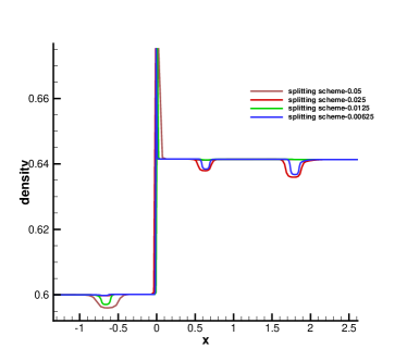
(a) density

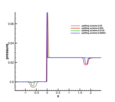
(b) pressure

Figure 2: The numerical solution of splitting scheme of Test1 at time $t=1.0s$ with different $h$: 0.05, 0.025, 0.0125, 0.00625. Left: density. Right: pressure.

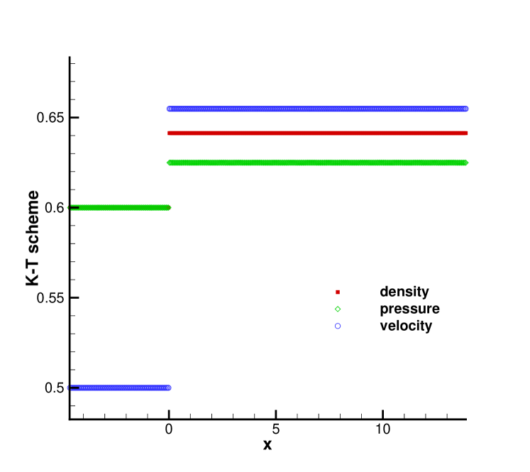
Figure 3: The numerical solution of K-T scheme of Test1 with $h=0.05$ at time $t=1.0s$.

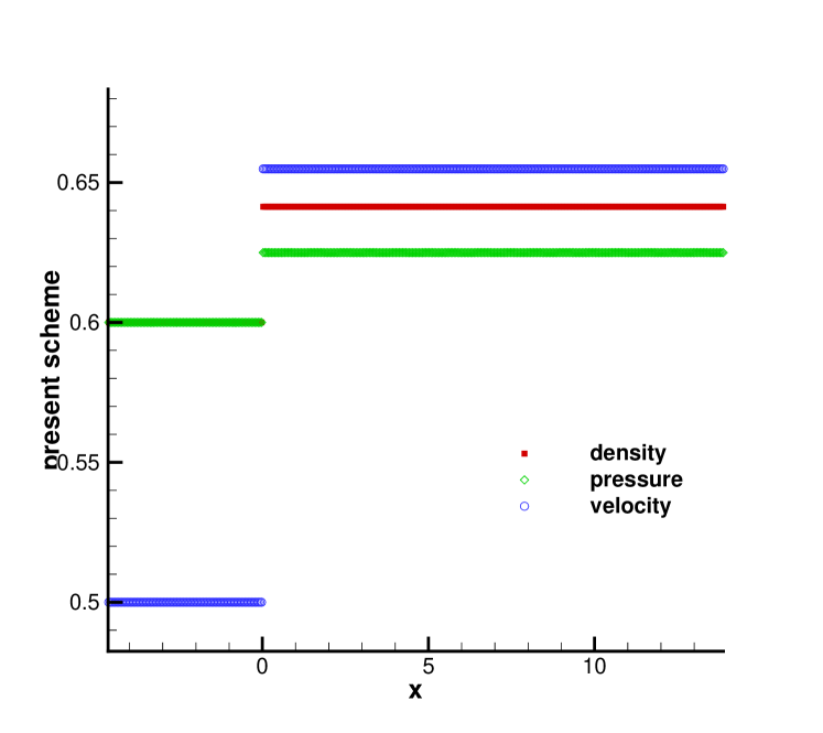
Figure 4: The numerical solution of present scheme of Test1 with $h=0.05$ at time $t=1.0s$.

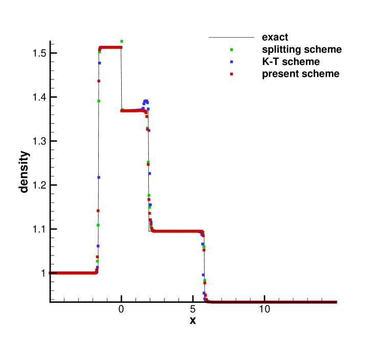
(a) density

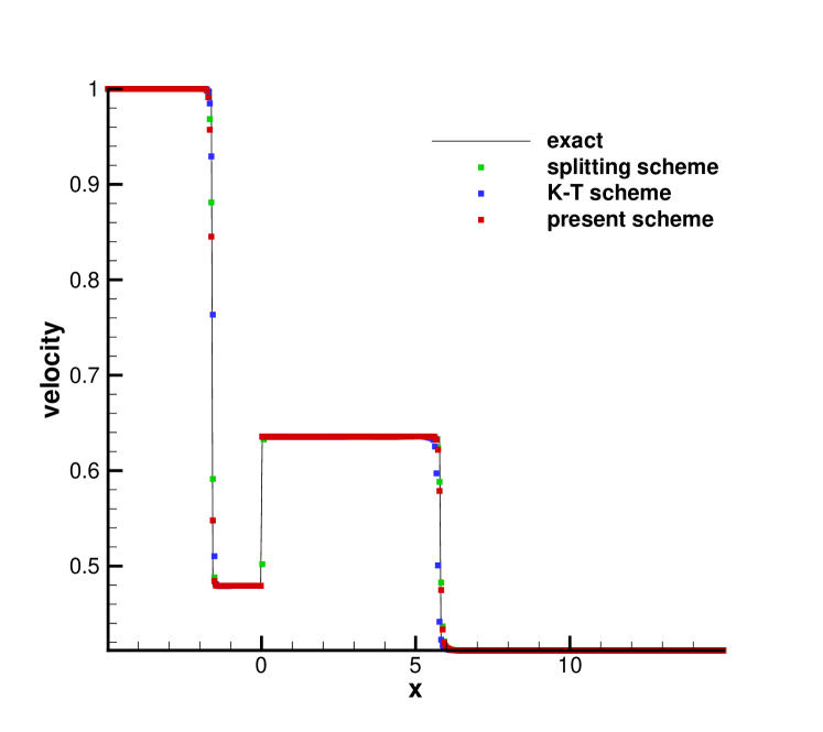
(b) velocity

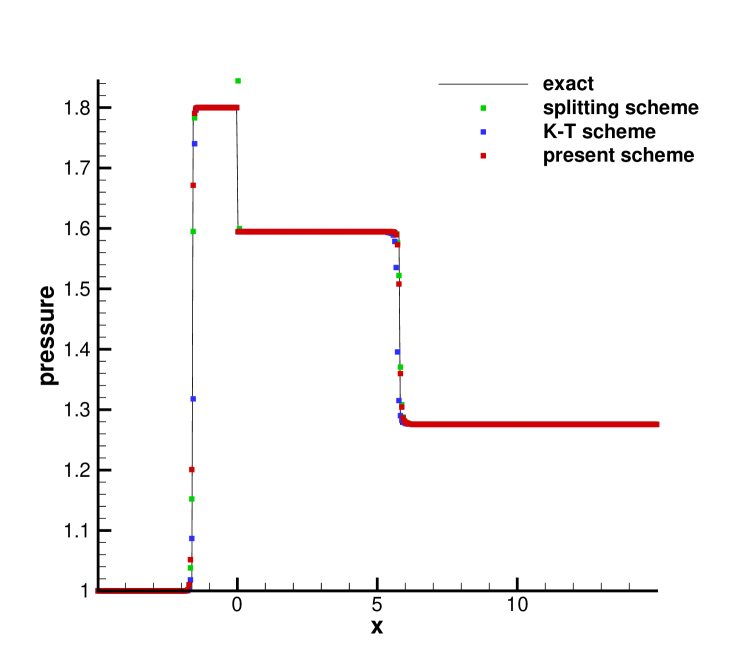
(c) pressure

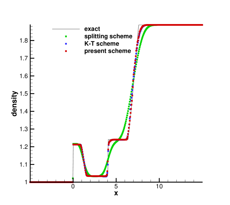
(d) density

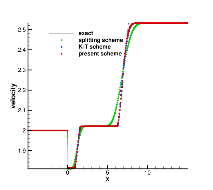
(e) velocity

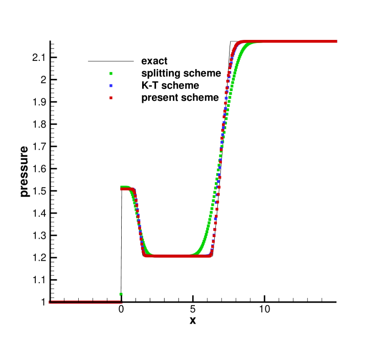
(f) pressure

Figure 5: Splitting scheme(green symbols), K-T scheme(blue symbols) and present scheme(red symbols) versus exact solutions(solid line) with $h=0.05$. Left column: Test2 and $t=3.0s$, right column: Test3 and $t=2.0s$. Top: density, middle: velocity, and bottom: pressure.

(a) density

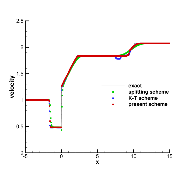
(b) velocity

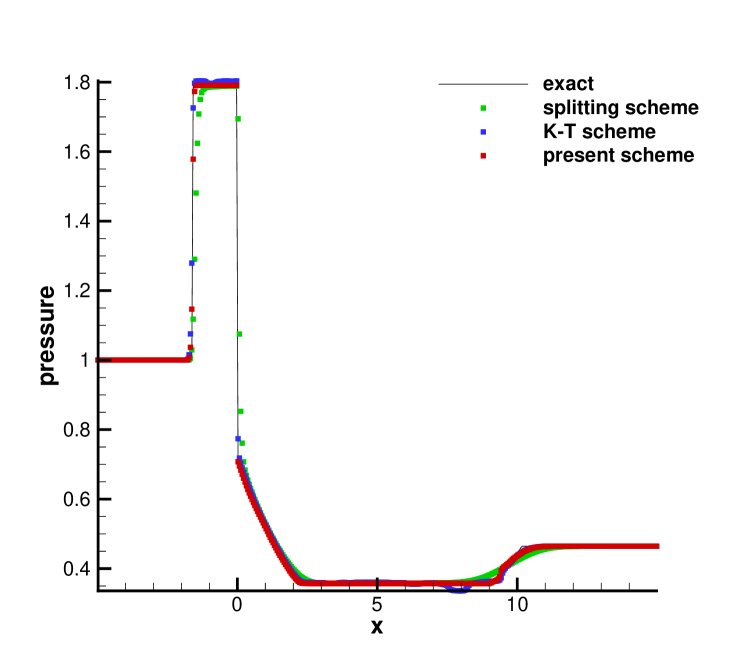
(c) pressure

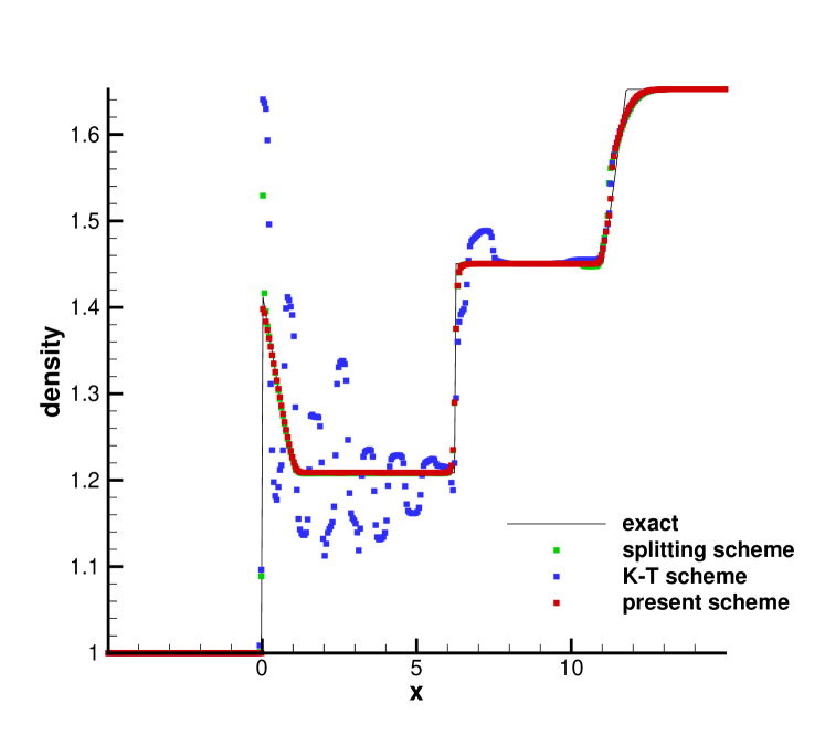
(d) density

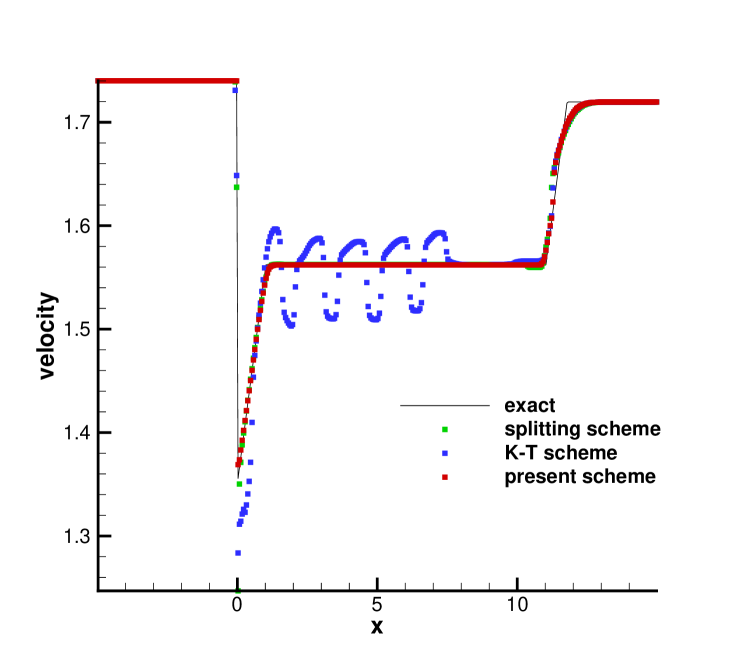
(e) velocity

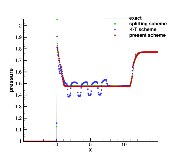
(f) pressure

Figure 6: Splitting scheme(green symbols), K-T scheme(blue symbols) and present scheme(red symbols) versus exact solutions(solid line) with $h=0.05$. Left column: Test4 and $t=3.0s$, right column: Test5 and $t=4.0s$. Top: density, middle: velocity, and bottom: pressure.

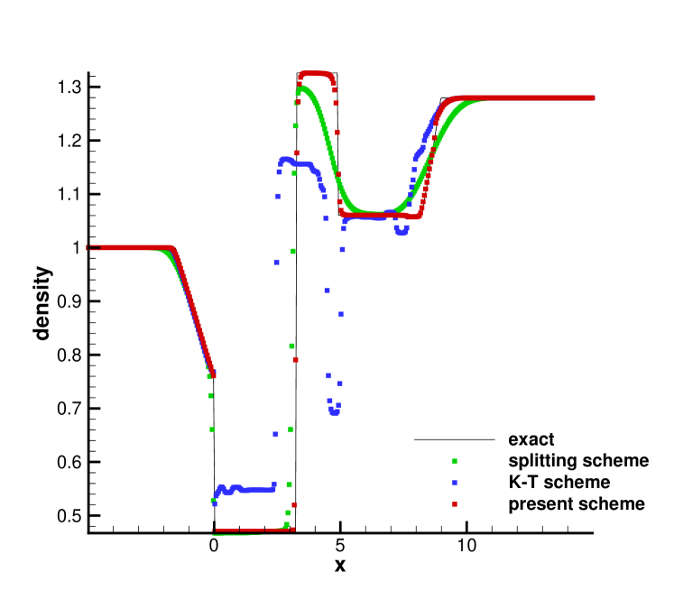
(a) density

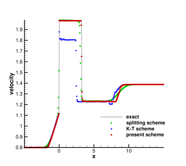
(b) velocity

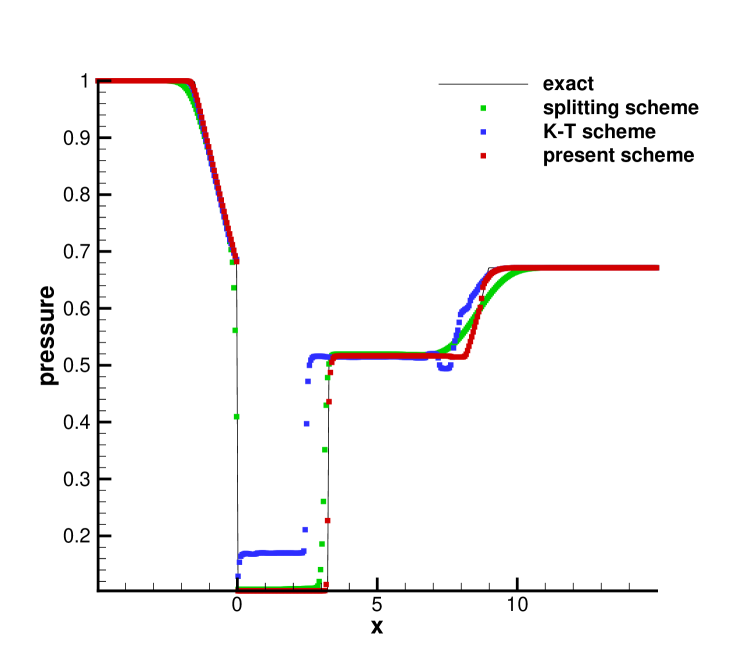
(c) pressure

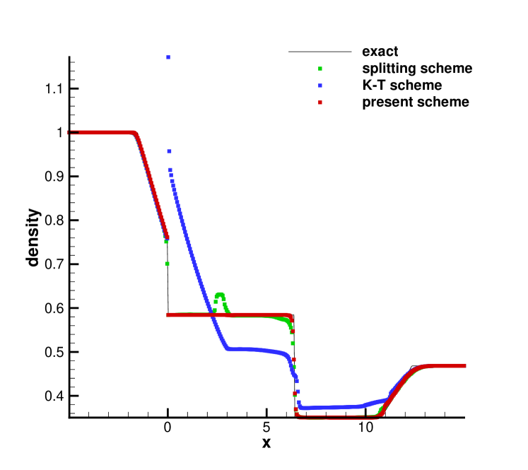
(d) density

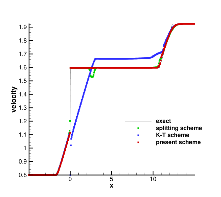
(e) velocity

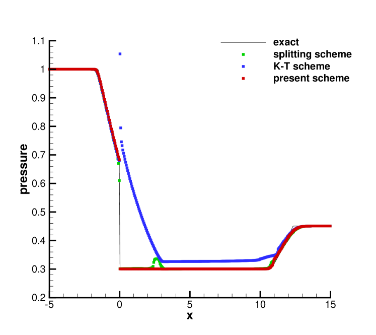
(f) pressure

Figure 7: Splitting scheme(green symbols), K-T scheme(blue symbols) and present scheme(red symbols) versus exact solutions(solid line) with $h=0.05$. Left column: Test6 and $t=4.0s$, right column: Test7 and $t=4.0s$. Top: density, middle: velocity, and bottom: pressure.

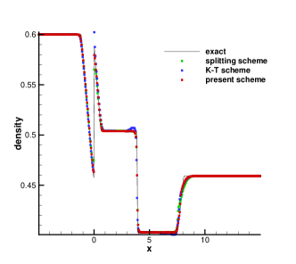
(a) density

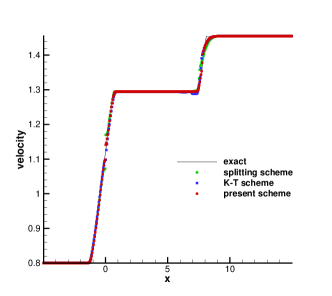
(b) pressure

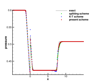
(c) pressure

Figure 8: Splitting scheme(green symbols), K-T scheme(blue symbols) and present scheme(red symbols) versus exact solutions(solid line) of Test8 with $h=0.05$ at time $t=3.0s$. Top left: density, Top right: velocity, and bottom: pressure.

The solutions of these tests are shown in Figure2, Figure4, Figure4, Figure5, Figure6, Figure7, Figure8.

In Test1, the initial value is a single stationary wave. We use this test to check whether the numerical scheme is well-balanced. As shown in Figure2, the splitting scheme is not well-balanced. the incorrect decomposition of the convection equation for the initial discontinuity leads to the numerical solution containing several incorrect perturbations, which associates with three classical characteristic domains. In addition, the numerical solution has overshoots near the origin due to the inability to maintain steady solutions. Furthermore, neither of these errors is significantly reduced as the grid is refined. The K-T scheme and our sover-based scheme are both well-balanced (see Figure4, Figure4).

The exact solutions for both Test 2 and Test 3 are non-choked, with the former having a Type1 structure and the latter a Type2. Figure5 gives the results of the three numerical schemes for these two tests, all of which are in good agreement with the exact solution. A disadvantage of the splitting scheme is that the numerical solution has overshoots in the vicinity of the stantionary wave. The K-T scheme has a slight oscillation at the downstream contact discontinuity in the numerical solution for Test2. The results of the present solver-based numerical scheme are free of both errors.

The structure of the exact solution of Test4 is Type3, which is choked. The results of the three numerical schemes are shown in the left figure of Figure6. The splitting scheme gives a relatively accurate approximation of the Riemann solution in each intermediate region, although its results have large numerical dissipation and overshoots near the stationary wave. For the K-T scheme, the numerical flux cannot satisfy the conditions in Theorem4.2 in this test. In order to make the K-T scheme work, we make some corrections, including the value of $I$ in (2.6) and (2.7) being set to zero if it is not solvable, and another branch of the stationary wave being adopted if the branch in (4.2) is not available. These corrections are also used in a few of the later tests. With these corrections, the K-T scheme works but there is still some non-physical oscillation. The present solver-based scheme approximates each elementary wave better and has less numerical dissipation.

The exact solution for Test5 is a choked solution of Type4 structure and the right figure of Figure6 shows the results for the three numerical schemes. The solution of the splitting scheme converges to the exact solution, but with larger overshoots near the stationary wave. The result of K-T scheme contains very large numerical oscillations, which we suspect, are due to the incorrect choice of branches of stationary wave curve. The state of exact solution to the right of the origin is sonic, so the state of numerical solution to the right of the origin may be perturbed around the sonic state. The perturbation of the numerical solution in the K-T scheme between the subsonic and supersonic states causes a change in the employed branch, which results in very large numerical oscillations. The results of the present solver-based scheme agrees well with the exact solution. Although our approximate Riemann solver ignores the Type4 structure, we achieve an approximation to the solution of this limit structure by the solution of the Type3 or Type2.

Test6 and Test7 are two choked solutions for $k<0$. The results of three schemes are shown in Figure7. The splitting method contains greater numerical dissipation than the other two schemes, and the numerical solution in the constant region to the right of the origin in Test7 contains oscillations. In both tests the K-T scheme gives incorrect results, and the results of our solver-based scheme agree well with the exact solution.

The last Test8 is an example of a choked solution for $k=0$. The exact solution has a rarefaction wave on each side of the origin in contact with it. The numerical solutions for all three schemes are capable of approximating the exact solution, as shown in Figure8. As can be seen from the density and pressure results, the present solver-based scheme works better than the other two schemes in the simulation of two rarefaction waves.

6 Conclusions

For Euler equations with a singular source, a solution-structure based approximate Riemann solver was proposed in this paper. The proposed solver is able to give the exact solution when the initial value is a single stationary wave and reasonable approximate solutions for different structures when the initial value is general. The numerical method based on our solver is not only well-balanced, but also can give numerical solutions in agreement with the exact solution in both non-extreme and extreme tests.

In one-dimensional problems we fixed the stationary singular source at a cell boundary. For one-dimensional equations with moving singular sources or for multidimensional equations, our solver can be directly generalised by means of reconstruction.

References

- [1] Remi Abgrall, P Bacigaluppi, and S Tokareva. A high-order nonconservative approach for hyperbolic equations in fluid dynamics. Computers & Fluids, 169:10–22, 2018.
- [2] Emmanuel Audusse, F Bouchut, Marie-Odile Bristeau, Rupert Klein, and B Perthame. A fast and stable well-balanced scheme with hydrostatic reconstruction for shallow water flows. SIAM Journal on Scientific Computing, 25(6):2050–2065, 2004.
- [3] Derek S Bale, Randall J Leveque, Sorin Mitran, and James A Rossmanith. A wave propagation method for conservation laws and balance laws with spatially varying flux functions. SIAM Journal on Scientific Computing, 24(3):955–978, 2003.
- [4] A. Bermudez and E. V. Ma. Upwind methods for hyperbolic conservation laws with source terms. Computers & Fluids, 23(8):1049–1071, 1994.
- [5] Roberto Bernetti, Vladimir A Titarev, and Eleuterio F Toro. Exact solution of the riemann problem for the shallow water equations with discontinuous bottom geometry. Journal of Computational Physics, 227(6):3212–3243, 2008.
- [6] Ramaz Botchorishvili, Benoit Perthame, and Alexis Vasseur. Equilibrium schemes for scalar conservation laws with stiff sources. Mathematics of Computation, 72(241):131–157, 2003.
- [7] Ramaz Botchorishvili and Olivier Pironneau. Finite volume schemes with equilibrium type discretization of source terms for scalar conservation laws. Journal of Computational Physics, 187(2):391–427, 2003.
- [8] Manuel Castro, José M Gallardo, Juan A López-GarcÍa, and Carlos Parés. Well-balanced high order extensions of godunov’s method for semilinear balance laws. SIAM Journal on Numerical Analysis, 46(2):1012–1039, 2008.
- [9] Manuel J Castro, Alberto Pardo Milanés, and Carlos Parés. Well-balanced numerical schemes based on a generalized hydrostatic reconstruction technique. Mathematical Models and Methods in Applied Sciences, 17(12):2055–2113, 2007.
- [10] Tung Chang and Ling Hsiao. The riemann problem and interaction of waves in gas dynamics. NASA STI/Recon Technical Report A, 90:44044, 1989.
- [11] Wan Cheng, Xisheng Luo, and MEH Van Dongen. On condensation-induced waves. Journal of fluid mechanics, 651:145–164, 2010.
- [12] Bernardo Cockburn, San Yih Lin, and Chi Wang Shu. Tvb runge-kutta local projection discontinuous galerkin finite element method for conservation laws iii: one-dimensional systems. Journal of Computational Physics, 1989.
- [13] Frédéric Coquel, Khaled Saleh, and Nicolas Seguin. A robust and entropy-satisfying numerical scheme for fluid flows in discontinuous nozzles. Mathematical Models and Methods in Applied Sciences, 24(10):2043–2083, 2014.
- [14] Dao Huy Cuong and Mai Duc Thanh. A godunov-type scheme for the isentropic model of a fluid flow in a nozzle with variable cross-section. Applied Mathematics and Computation, 256:602–629, 2015.
- [15] Pratik Das and HS Udaykumar. A sharp-interface method for the simulation of shock-induced vaporization of droplets. Journal of Computational Physics, 405:109005, 2020.
- [16] Pratik Das and HS Udaykumar. A simulation-derived surrogate model for the vaporization rate of aluminum droplets heated by a passing shock wave. International Journal of Multiphase Flow, 130:103299, 2020.
- [17] Pratik Das and HS Udaykumar. Sharp-interface calculations of the vaporization rate of reacting aluminum droplets in shocked flows. International Journal of Multiphase Flow, 134:103442, 2021.
- [18] Stefan Fechter, Claus-Dieter Munz, Christian Rohde, and Christoph Zeiler. Approximate riemann solver for compressible liquid vapor flow with phase transition and surface tension. Computers & Fluids, 169:169–185, 2018.
- [19] David L George. Augmented riemann solvers for the shallow water equations over variable topography with steady states and inundation. Journal of Computational Physics, 227(6):3089–3113, 2008.
- [20] Irene Gómez-Bueno, Manuel J Castro, and Carlos Parés. High-order well-balanced methods for systems of balance laws: a control-based approach. Applied Mathematics and Computation, 394:125820, 2021.
- [21] GOSSE and LAURENT. A well-balanced scheme using non-conservative products designed for hyperbolic systems of conservation laws with source terms. Mathematical Models & Methods in Applied Sciences, 11(02):339–365, 2008.
- [22] Gottlieb, Sigal, Shu, and Chi-Wang. Strong stability-preserving high-order time discretization methods. Siam Review, 2001.
- [23] JM Greenberg, AY Leroux, R Baraille, and A Noussair. Analysis and approximation of conservation laws with source terms. SIAM Journal on Numerical Analysis, 34(5):1980–2007, 1997.
- [24] Joshua M Greenberg and Alain-Yves LeRoux. A well-balanced scheme for the numerical processing of source terms in hyperbolic equations. SIAM Journal on Numerical Analysis, 33(1):1–16, 1996.
- [25] Timon Hitz, Matthias Heinen, Jadran Vrabec, and Claus-Dieter Munz. Comparison of macro-and microscopic solutions of the riemann problem i. supercritical shock tube and expansion into vacuum. Journal of Computational Physics, 402:109077, 2020.
- [26] Ryan W Houim and Kenneth K Kuo. A ghost fluid method for compressible reacting flows with phase change. Journal of Computational Physics, 235:865–900, 2013.
- [27] Shi Jin. A steady-state capturing method for hyperbolic systems with geometrical source terms. ESAIM: Mathematical Modelling and Numerical Analysis, 35(4):631–645, 2001.
- [28] Shi Jin and Xin Wen. Two interface-type numerical methods for computing hyperbolic systems with geometrical source terms having concentrations. SIAM Journal on Scientific Computing, 26(6):2079–2101, 2005.
- [29] Kenneth Karlsen, Siddhartha Mishra, and Nils Risebro. Well-balanced schemes for conservation laws with source terms based on a local discontinuous flux formulation. Mathematics of Computation, 78(265):55–78, 2009.
- [30] Dietmar Kröner, Philippe G LeFloch, and Mai-Duc Thanh. The minimum entropy principle for compressible fluid flows in a nozzle with discontinuous cross-section. ESAIM: Mathematical Modelling and Numerical Analysis, 42(3):425–442, 2008.
- [31] Dietmar Kröner and Mai Duc Thanh. Numerical solutions to compressible flows in a nozzle with variable cross-section. SIAM journal on numerical analysis, 43(2):796–824, 2005.
- [32] Jaewon Lee and Gihun Son. A sharp-interface level-set method for compressible bubble growth with phase change. International Communications in Heat and Mass Transfer, 86:1–11, 2017.
- [33] Moon Soo Lee, Amir Riaz, and Vikrant Aute. Direct numerical simulation of incompressible multiphase flow with phase change. Journal of Computational Physics, 344:381–418, 2017.
- [34] Philippe G Lefloch and Mai Duc Thanh. The riemann problem for fluid flows in a nozzle with discontinuous cross-section. Communications in Mathematical Sciences, 1(4):763–797, 2003.
- [35] Philippe G LeFloch and Mai Duc Thanh. A godunov-type method for the shallow water equations with discontinuous topography in the resonant regime. Journal of Computational Physics, 230(20):7631–7660, 2011.
- [36] Alain Yves Leroux. Riemann solvers for some hyperbolic problems with a source term. In ESAIM: Proceedings, volume 6, pages 75–90. EDP Sciences, 1999.
- [37] Randall J LeVeque. Balancing source terms and flux gradients in high-resolution godunov methods: the quasi-steady wave-propagation algorithm. Journal of computational physics, 146(1):346–365, 1998.
- [38] Randall J LeVeque and Helen C Yee. A study of numerical methods for hyperbolic conservation laws with stiff source terms. Journal of computational physics, 86(1):187–210, 1990.
- [39] Gang Li, Jiaojiao Li, Shouguo Qian, and Jinmei Gao. A well-balanced ader discontinuous galerkin method based on differential transformation procedure for shallow water equations. Applied Mathematics and Computation, 395:125848, 2021.
- [40] Tian Long, Jinsheng Cai, and Shucheng Pan. A fully conservative sharp-interface method for compressible mulitphase flows with phase change. arXiv preprint arXiv:2110.07995, 2021.
- [41] Miltiadis V Papalexandris, Anthony Leonard, and Paul E Dimotakis. Unsplit schemes for hyperbolic conservation laws with source terms in one space dimension. Journal of Computational Physics, 134(1):31–61, 1997.
- [42] Thomas Paula, Stefan Adami, and Nikolaus A Adams. Analysis of the early stages of liquid-water-drop explosion by numerical simulation. Physical Review Fluids, 4(4):044003, 2019.
- [43] Youngho Suh and Gihun Son. A level-set method for simulation of a thermal inkjet process. Numerical Heat Transfer, Part B: Fundamentals, 54(2):138–156, 2008.
- [44] Mai Duc Thanh. The riemann problem for a nonisentropic fluid in a nozzle with discontinuous cross-sectional area. SIAM Journal on Applied Mathematics, 69(6):1501–1519, 2009.
- [45] Mai Duc Thanh. Numerical treatment in resonant regime for shallow water equations with discontinuous topography. Communications in Nonlinear Science and Numerical Simulation, 18(2):417–433, 2013.
- [46] Nguyen Xuan Thanh, Mai Duc Thanh, and Dao Huy Cuong. Dimensional splitting well-balanced schemes on cartesian mesh for 2d shallow water equations with variable topography. Bulletin of the Iranian Mathematical Society, pages 1–28, 2021.
- [47] Eleuterio F Toro. Riemann solvers and numerical methods for fluid dynamics: a practical introduction. Springer Science & Business Media, 2013.
- [48] Y. Xing and C. W. Shu. High order well-balanced finite volume weno schemes and discontinuous galerkin methods for a class of hyperbolic systems with source terms. Journal of Computational Physics, 214(2):567–598, 2006.
- [49] Yang Yang and Chi-Wang Shu. Discontinuous galerkin method for hyperbolic equations involving delta-singularities: negative-order norm error estimates and applications. Numerische Mathematik, 124(4):753–781, 2013.
- [50] Changsheng Yu, Tiegang Liu, and Chengliang Feng. Riemann problem of euler equations with singular sources. arXiv preprint arXiv:2203.04512, 2022.