Overcoming Temptation:
Incentive Design For Intertemporal Choice

Abstract

Individuals are often faced with temptations that can lead them astray from long-term goals. We’re interested in developing interventions that steer individuals toward making good initial decisions and then maintaining those decisions over time. In the realm of financial decision making, a particularly successful approach is the prize-linked savings account: individuals are incentivized to make deposits by tying deposits to a periodic lottery that awards bonuses to the savers. Although these lotteries have been very effective in motivating savers across the globe, they are a one-size-fits-all solution. We investigate whether customized bonuses can be more effective. We formalize a delayed-gratification task as a Markov decision problem and characterize individuals as rational agents subject to temporal discounting, a cost associated with effort, and fluctuations in willpower. Our theory is able to explain key behavioral findings in intertemporal choice. We created an online delayed-gratification game in which the player scores points by selecting a queue to wait in and then performing a series of actions to advance to the front. Data collected from the game is fit to the model, and the instantiated model is then used to optimize predicted player performance over a space of incentives. We demonstrate that customized incentive structures can improve an individual’s goal-directed decision making.

Significance Statement

Individuals are often tempted to abandon long-term goals (e.g., weight loss) by enticements that provide immediate reward (e.g., a piece of cake). We use computational models of decision making to determine personalized interventions that allow an individual to overcome temptation and improve long-term outcomes. We formalize a theory in which individuals make a series of choices to persist toward long-term goals or defect and obtain an immediate reward. The theory is used to determine a limited schedule of incentives that maximizes expected outcomes. We conduct experiments with a simulated line-waiting task that show the theory’s potential.

Should you go hiking today or work on that manuscript? Should you have a slice of cake or stick to your diet? Should you upgrade your flat-screen TV or contribute to your retirement account? Individuals are regularly faced with temptations that lead them astray from long-term goals. These temptations all reflect an underlying challenge in behavioral control that involves choosing between actions leading to small but immediate rewards and actions leading to large but delayed rewards. We introduce a formal model of delayed-gratification decision tasks and use the model to optimize behavior by designing incentives to assist individuals in achieving long-term goals.

Consider the serious predicament with retirement planning in the United States. Only 55% of working-age households have retirement account assets—whether an employer-sponsored plan or an IRA—and the median account balance for near-retirement households is $14,500. Even considering households’ net worth, $2/3$ fall short of conservative savings targets based on age and income [2]. Balances in retirement accounts for age-60 participants are reduced by 31% due to leakage, including cash-outs, hardship withdrawals, and the failure to repay loans [3]. In 2013, the US government and nonprofits spent $670M on financial education, yet financial literacy accounts for a minuscule 0.1% of the variance in financial outcomes [4].

One technique that has been extremely successful in encouraging savings, primarily in Europe and the developing world but more recently in the US as well, is the prize linked savings account (PLSA) [5, 6]. The idea is to pool a fraction of the interest from all depositors to fund a prize awarded by periodic lotteries. Just as ordinary lotteries entice individuals to purchase tickets, the PLSA encourages individuals to save. Disregarding the fact that lotteries function in part because individuals overvalue low-probability gains [7], the core of the approach is to offer savers the prospect of short-term payoffs in exchange for them committing to the long term. Although the account yields a lower interest rate to fund the lottery, the PLSA increases the net expected account balance due to greater commitment to participation.

The PLSA is a one-size-fits-all solution. A set of incentives that work well for one individual or one subpopulation may not be optimal for another. In this article, we investigate approaches to customizing incentives to an individual or a subpopulation with the aim of achieving greater adherence to long-term goals and ultimately, better long-term outcomes for the participants. Our approach involves: (1) building a model to characterize the behavior of an individual or group, (2) fitting the model with behavioral data, (3) using the model to determine an incentive structure that optimizes outcomes, and (4) validating the model by showing better outcomes with model-derived incentives than with alternative incentive structures.

Intertemporal Choice

Saving for retirement and other delayed-gratification tasks involve choosing between alternatives that produce gains and losses at different points in time, or intertemporal choice. How an individual interprets delayed consequences influences the utility or value associated with a decision. When consequences are discounted with the passage of time, decision making leans toward more immediate gains and more distant losses. The delay discounting task is often used to study intertemporal choice [8]. Individuals are asked to choose between two alternatives, e.g., $1 today versus $$X$ in $Y$ days. By identifying the $X$ that yields subjective indifference for a given $Y$, one can estimate an individual’s discounting of future outcomes. Discount rates vary across individuals yet show stability over extended periods of time [9].

This paradigm involves a single, hypothetical decision and reveals the intrinsic future value of an outcome. However, it does not address the temporal dynamics of behavior over an extended period of time in delayed-gratification tasks. In such tasks, once an initial decision is made to wait for a large reward, individuals are permitted to abandon the decision at any instant in favor of the small immediate reward. For example, in the classic marshmallow test [10], children are seated at a table with a single marshmallow. They are allowed to eat the marshmallow, but if they wait while the experimenter steps out of the room, they will be offered a second marshmallow when the experimenter returns. In this scenario, children continually contemplate whether to eat the marshmallow or wait for two marshmallows. Their behavior depends not only on the hypothetical discounting of future rewards but on the individual’s willpower [11]—their ability to maintain focus on the larger reward and not succumb to temptation before the experimenter returns. Defection at any moment eliminates the possibility of the larger reward.

The marshmallow test achieved renown not only because it is claimed to be predictive of later life outcomes [12], but because it is analogous to many situations involving delayed gratification. Like the marshmallow test, some of these situations have an unspecified time horizon (e.g., exercise, waiting for an elevator, spending during retirement). However, others have a known horizon (e.g., avoiding snacks before dinner, saving for retirement, completing a college degree). Our work addresses the case of a known or assumed horizon.

Whether or not the horizon is known, delayed-gratification tasks may additionally be characterized in terms of the number of opportunities to obtain the delayed reward. The marshmallow test is one shot, but many true-to-life scenarios have an iterated nature. For example, in retirement planning, the failure to contribute to the account one month does not preclude contributing the next month. Another intuitive example involves allocating time within a work day. One must choose between tasks that are brief and provide a moment of satisfaction (e.g., answering email) and tasks that will take a long time to complete but will eventually yield a sense of accomplishment (e.g., writing a manuscript). Our work addresses both one-shot and iterated delayed-gratification tasks. For such tasks, we’re interested in developing personalized interventions that assist individuals both in making good initial decisions and in maintaining those decisions over time.

Theories of Intertemporal Choice

Nearly all previous conceptualizations of intertemporal choice have focused on the shape of the discounting function and the initial ‘now versus later’ decision, not the time course. One exception is the work of McGuire and Kable [13] who frame failure to postpone gratification as a rational, utility-maximizing strategy when the time at which future outcomes materialize is uncertain. Our theory is complementary in providing a rational account in the known time horizon situation.

When one considers the time course of delaying gratification—the need to recommit to the decision and not succumb to temptation—the appropriate framework for modeling behavior is that of sequential decision making. There is a rich literature on modeling human sequential decision-making using the formalism of Markov decision processes [MDPs; e.g., 14, 15, 16, 17, 18, 19, 20, 21]. In this framework, human behavior is interpreted with respect to the behavior of a rational agent, i.e., an agent following an optimal (reward maximizing) policy. The optimal policy is determined via dynamic programming or reinforcement learning [22], both of which can accommodate discounting of future outcomes. Even when human decisions deviate from those of the rational agent, the modeling framework is nonetheless valuable if additional bounded rationality assumptions allow it to account for human performance [23, 24, 25].

The MDP framework, which allows rewards of various magnitudes to be realized at different points in time, is well suited for modeling intertemporal choice. Kurth-Nelson and Redish [26, 27] explore a model of precommitment in decision making as a means of preventing impulsive defections. Their model addresses the initial decision to commit rather than the ongoing possibility of defection. Lieder et al. [18], whose work is closest to our own, address a class of intertemporal-choice tasks—not exactly delayed gratification tasks—in which individuals have to choose between difficult and time consuming work assignments that eventually lead to a large payout (strategic route planning, essay writing) and easy alternatives that thwart obtaining the eventual payout (making an impulsive choice, watching a YouTube video, abandoning the experiment). They use the MDP theoretical framework to develop an optimal gamification approach to help individuals avoid procrastination and to achieve future-minded goals. We further discuss this interesting work and its relation to ours later and in the Supplementary Materials.

Formalizing Delayed-Gratification Tasks as a Markov Decision Problem

In this section, we formalize a delayed-gratification task as a Markov decision problem, which we will refer to as the DGMDP. We assume time to be quantized into discrete steps and we focus on situations with a known or assumed time horizon, denoted $\tau$. At any step, the agent may defect and collect a small reward, or the agent may persist to the next step, eventually collecting a large reward at step $\tau$. We use $\mu_{\textrm{\tiny SS}}$ and $\mu_{\textrm{\tiny LL}}$ to denote the smaller sooner (SS) and larger later (LL) rewards.

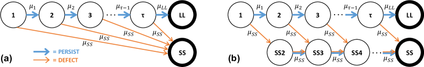
Figure 1: Finite-state environment formalizing (a) the one-shot delayed-gratification task; (b) an efficient approximation to the iterated delayed-gratification task, suitable when episodes are independent of one another and reward rate is to be maximized.

Figure 1a shows a finite-state representation of the one-shot task with terminal states LL and SS that correspond to resisting and succumbing to temptation, respectively, and states for each time step between the initial and final times, $t\in\{1,2,...,\tau\}$. Rewards are associated with state transitions. The possibility of obtaining intermediate rewards during the delay period is annotated via $\bm{\mu}_{1:\tau-1}\equiv\{\mu_{1},...,\mu_{\tau-1}\}$, which we return to later. With exponential discounting, rewards $n$ steps ahead are devalued by a factor of $\gamma^{n}$, $0\leq\gamma<1$.

Given the DGMDP, an optimal decision sequence is trivially obtained by value iteration. However, this sequence is a poor characterization of human behavior. With no intermediate rewards ($\smash{\bm{\mu}_{1:\tau-1}=\mathbf{0}}$), it takes one of two forms: either the agent defects at $t=1$ or the agent persists through $t=\tau$. In contrast, individuals will often persist some time and then defect, and when placed into the same situation repeatedly, behavior is nondeterministic. For example, replicability on the marshmallow test is quite modest, with $\rho<0.30$ [28]. The discrepancy between human delayed-gratification behavior and the optimal decision-making framework might indicate an incompatibility. However, we prefer a bounded-rationality perspective on human cognition according to which behavior is cast as optimal but subject to operational constraints [23]. We postulate two specific constraints.

1. The decision-making framework is one component of a cognitive architecture. When modeling an isolated component, it is common to treat factors external to the component as a noise source that contributes to behavioral variability. Here, we introduce a one-dimensional Gaussian process, $W=\{W_{t}\}$, with

   $$w_{1}~{}\sim~{}\mathrm{Gaussian}(0,\sigma_{1}^{2})\qquad\text{and}\qquad w_{t}~{}\sim~{}\mathrm{Gaussian}(w_{t-1},\sigma^{2}).$$

   We suppose that this quantity, which we refer to as the bias, modulates an individual’s subjective value of defecting at step $t$:

   $$Q(\{t,w\},{\text{\sc defect}})=\mu_{\textrm{\tiny SS}}-w,$$ (1)

   where $Q(\bm{s},a)$ denotes the value associated with performing action $a$ in state $\bm{s}$, and the state space consists of the discrete step $t$ and the continuous bias $w$.

2. Behavioral, economic, and neural accounts of decision making suggest that effort carries a cost, that rewards are weighed against the effort required to obtain it [e.g., 29], and that the avoidance of effort has mechanistic and rational bases [30]. Without concerning ourselves with these bases, we incorporate into the model an effort cost, $\mu_{\textrm{\tiny E}}$, that is associated with persevering:

   $$Q(\{t,w\},{\text{\sc persist}})=\begin{cases}\mu_{\textrm{\tiny E}}+\mu_{t}+\gamma~{}\mathbb{E}_{W_{t+1}|W_{t}=w}V(t+1,w_{t+1})&\text{for }t<\tau\\ \mu_{\textrm{\tiny LL}}&\text{for }t=\tau\end{cases}$$ (2)

   $$\text{where}~{}~{}V(t,w)\equiv\mathrm{max}_{a}~{}Q(\{t,w\},a).$$ (3)

With these two constraints, we will show that the model not only has adequate expressive power to fit behavioral data, but also has the explanatory power to predict experimental outcomes.

The one-shot DGMDP in Figure 1a can be extended to model the iterated task, even when there is variability in the reward ($\mu_{\textrm{\tiny LL}}$) or duration ($\tau$) across episodes (see Figure Supp-1a,b). It is straightforward to show that the solution to the iterated DGMDPs is identical to the solution to the simpler and more tractable one-shot DGMDP in Figure 1b under certain constraints (see Supplementary Information). Essentially, Figure 1b models the choice between the LL reward or a sequence of SS rewards matched in total number of steps, effectively comparing the reward rates for LL and SS, the critical variables in the iterated DGMDP.

To summarize, we have formalized one-shot and iterated delayed-gratification task with known horizon as a Markov decision problem with parameters $\Theta_{\mathrm{task}}\equiv\{\tau,\mu_{\textrm{\tiny SS}},\mu_{\textrm{\tiny LL}},\bm{\mu}_{1:\tau-1}\}$, and a constrained rational agent parameterized by $\Theta_{\mathrm{agent}}\equiv\{\gamma,\sigma_{1},\sigma,\mu_{\textrm{\tiny E}}\}$. We now turn to solving the DGMDP and characterizing its properties.

Solving The Delayed-Gratification Markov Decision Problem (DGMDP)

The simple structure of the environment allows for a backward-induction solution to the Bellman equation (Equation 2). Although the bias $w$ precludes an analytical solution for the value $V(t,w)$, we construct a piecewise-linear approximation over $w$ for each step $t$, as described in the Supplementary Materials. Figure 2a shows the value as a function of bias at each step of an eight step DGMDP with an LL reward twice that of the SS reward, like the canonical marshmallow test. Both the exact value-function formulation obtained by discretizing bias and the corresponding piecewise-linear approximation (Equation Supp-6) are presented in colored and black lines, respectively.

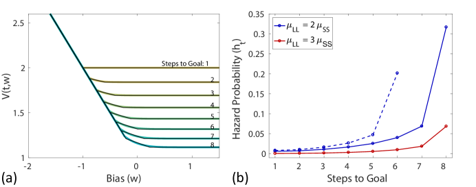
Figure 2: (a) Value function for a DGMDP with $\tau=8$, $\sigma=.25$, $\sigma_{1}=.50$, $\gamma=.92$, $\mu_{\textrm{\tiny E}}=\mu_{t}=0$, $\mu_{\textrm{\tiny LL}}=2$, $\mu_{\textrm{\tiny SS}}=1$, exact (colored curves) and piecewise linear approximation (black lines). (b) Hazard functions for the parameterization in (a) (solid blue curve), with a higher level of LL reward (red curve), and with a shorter delay period, $\tau=6$ (dashed blue curve).

Using the value function, we can characterize the agent’s behavior in the DGMDP via the likelihood of defecting at various steps. With $D$ denoting the defection step, we have the hazard probability,

$$h_{t}\equiv P(D=t|D\geq t)\equiv P(W_{t}<w_{t}^{*}|W_{1}\geq w_{1}^{*},...,W_{t-1}\geq w_{t-1}^{*}),$$ (4)

where $w^{*}$ is the bias threshold that yields action indifference,

$$Q(t,w^{*};{\text{\sc defect}})=Q(t,w^{*};{\text{\sc persist}}).$$

Estimation of Equation 4 is discussed in the Supplementary Materials.

The solid blue curve in Figure 2b shows the hazard function for the DGMDP in Figure 2a. Defection rates drop as the agent approaches the goal. Defection rates also scale with the LL reward, as illustrated by the contrast between the solid blue and red curves. Finally, defection rates depend both on relative and absolute steps to goal: contrasting the solid and dashed blue curves, corresponding to $\tau=8$ and $\tau=6$, respectively, the defection rate at a given number of steps from the goal depends on $\tau$. We show shortly that human data exhibit this same qualitative property. Interestingly, the random walk in bias is critical in obtaining this property. When bias is independent from step to step, i.e., $w_{t}~{}\sim~{}\mathrm{Gaussian}(0,\sigma^{2})$, defection rates depend only on absolute steps to goal. Thus, the moment-to-moment nonzero autocorrelation is essential for modeling human behavior.

Behavioral Phenomena Explained

We consider the solution of the DGMDP as a rational theory of human cognition. It is meant to explain both an individual’s initial choice (“Should I open a retirement account?”) as well as the temporal dynamics of sustaining that choice (“Should I withdraw the funds to buy a car?”).

Our theory explains two key phenomena in the literature. First, failure on a DG task is sensitive to the relative magnitudes of the SS and LL rewards [31]. Figure 2b presents hazard functions for two reward magnitudes. The probability of obtaining the LL reward is greater with $\mu_{\textrm{\tiny LL}}/\mu_{\textrm{\tiny SS}}=3$ than with $\mu_{\textrm{\tiny LL}}/\mu_{\textrm{\tiny SS}}=2$. Figure 2b can also accommodate the finding that environmental reliability and trust in the experimenter affect outcomes in the marshmallow test [32]: in unreliable or nonstationary environments, the expected LL reward is lower than the advertised reward, and the DGMDP is based on reward expectations. Second, a reanalysis of data from a population of children performing the marshmallow task shows a declining hazard rate over the task period of 7 minutes [13]. The rapid initial drop in the empirical curve looks remarkably like the curves in Figure 2b. One might interpret this phenomenon as a finish-line effect: the closer one gets to a goal, the greater is the commitment to achieve the goal. However, the model suggests that this behavior arises not from abstract psychological constructs but because of correlations in bias over time: if an individual starts down the path to an LL reward, the individual’s bias at that point must be high. The posterior bias distributions reflect the elimination of individuals with low momentary bias, which contributes to the declining hazard rate. Also contributing is the exponential increase in value of the discounted LL reward as the agent advances through the DGMDP. McGuire and Kable [13] explain the empirical hazard function via a combination of uncertainty in the time horizon and time-fluctuating discount rates. Our theory shows that these strong assumptions are not necessary, and our theory can address situations with a well delineated horizon such as retirement saving. Additionally, our theory aims to move beyond population data and explain the granular dynamical behavior of an individual, as we demonstrate in experiments to follow.

Optimizing Incentives

We explore a mechanism-design approach [33] aimed at steering individuals toward improved long-term outcomes. We ask whether we can provide incentives or bonuses to rational value-maximizing agents that will increase their expected reward. In contrast to [18], the bonuses are actually paid out and are constrained so as not to “print money,” as we describe shortly.

We first address an investment scenario roughly analogous to a prize-linked savings account (PLSA). Suppose an individual has $x$ dollars which they can deposit into a bank account earning interest at rate $r$, compounded annually. At the start of each year, they decide whether to continue saving (persist) or to withdraw and spend their entire savings with interest accumulated thus far (defect). Our goal to assist them in maximizing the profit they reap over $\tau-1$ years from their initial investment. Our incentive mechanism is a a schedule of lotteries. We refer to expected lottery distributions as bonuses, even though they are funded through the interest earned by a population of individuals, like the prizes of the PLSA.

With $\mu_{t}$ denoting the bonus awarded in year $t$ and $\bm{\mu}_{1:\tau-1}$ denoting the set of scheduled bonuses, our goal as mechanism designers is to identify the schedule that maximizes the expected net accumulation from an individual’s investment:

$$\textstyle{\bm{\mu}^{*}_{1:\tau-1}=\text{argmax}_{\bm{\mu}_{1:\tau-1}}\sum_{t=1}^{\tau}P(D=t|\gamma,\bm{\mu}_{1:\tau-1})\left[b_{t}+\sum_{t^{\prime}=1}^{t-1}\mu_{t^{\prime}}\right]},$$ (5)

where $b_{t}$ is the amount banked at the start of year $t$, with $b_{1}=x$ and $b_{t+1}=(1+r)(b_{t}-\mu_{t})$, and $D$ is the year of defection, where $D=1$ represents immediate defection and $D=\tau$ represents the the account reaching maturity. Defection probabilities are obtained from the theory (Equation 4).

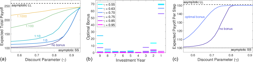
Figure 3: Bonus optimization for an agent with $\sigma_{1}=50$, $\sigma=30$, $\mu_{\textrm{\tiny E}}=0$, and $\gamma\in[0.55,0.95]$. (a) Expected payoff for the one-shot DGMDP for various bonus scenarios, including no bonus and optimal bonuses with lottery odds 1:0, 1:10, 1:100, and 1:1000. In these simulations, the interest-accrual setting is used to constrain bonuses and payoffs. (b) For the certain win (1:0) lottery with an initial fund of $x=100$, optimal bonus at each step for various $\gamma$. The optimal bonus is expressed as the percentage of initial pool of funding. (c) Expected payoff per time step for the iterated DGMDP for the bonus-limit setting used to constrain bonuses and payoffs.

To illustrate this approach, we conducted a simulation with discount factor $\smash{\gamma\in[0.55,0.95]}$, $\smash{\tau=10}$ year horizon, annual interest rate $\smash{r=0.1}$, and initial bank $\smash{x=100}$, comparing an agent’s expected accumulation without bonuses and with optimal bonuses. Optimization is via direct search using the simplex algorithm over unconstrained variables $p_{t}\equiv\text{logit}(\mu_{t}/b_{t})$, representing the proportion of the bank being distributed as a bonus.

We first consider the case of deterministic bonuses: the agent receives bonus $\mu_{t}$ in year $t$ with certainty. Figure 3a shows the expected payoff as a function of an agent’s discount factor $\gamma$ for the scenario with no bonuses (purple curve) versus optimal bonuses awarded with probability 1.0 (light blue curve, labeled with the odds of a bonus being awarded, ‘1:0’). For reference, the asymptotic SS and LL payoffs are shown with dotted and dashed lines, respectively.

With high discounting, this simulation yields a roughly $10\%$ improvement in an individual’s expected accumulation by providing bonuses at the end of the early years and going into the final year (Figure 3b). Bonuses are recommended only when the gain from encouraging persistence beats the loss of interest on an awarded bonus. With low discounting, the model optimization recommends no bonuses. Thus, the simulation recommends different incentives to individuals depending on their discount factors.

Now consider a lottery such as that conducted for the PLSA. If individuals operate based on expected returns, an uncertain lottery with odds 1:$\alpha$ and payoff $(\alpha+1)\mu_{t}$ would be equivalent to a certain payoff of $\mu_{t}$. However, as characterized by prospect theory [7], individuals overweight low probability events. Using median parameter estimates from cumulative prospect theory [34] to infer subjective probabilities on lotteries with 1:10, 1:100, and 1:000 odds, we optimize bonuses for these cases. As depicted by the three upper curves in Figure 3a, lotteries such as the PLSA can significantly boost the benefit of incentive optimization.

Lotteries and interest accrual are not suitable for all delayed-gratification tasks. For instance, one would not wish to encourage a dieter by offering a lottery for a 50-gallon tub of ice cream or the promise of a massive all-one-can-eat dessert buffet at the conclusion of the diet. To demonstrate the flexibility of our framework, we posit a bonus-limit setting as an alternative to the interest-accrual setting in which up to $n_{b}$ bonuses of fixed size can be awarded and the optimization determines the time steps at which they are awarded. We conducted a simulation with the iterated DGMDP (Figure 1b) using $\smash{\gamma\in[0.55,0.95]}$, $\smash{\tau=10}$, awarding of $n_{b}\leq 4$ bonuses each of value 50, $\smash{\mu_{\textrm{\tiny SS}}=100}$, and $\smash{\mu_{\textrm{\tiny LL}}=150\tau-50n_{b}}$. Multiple bonuses could be awarded in the same step, but bonuses were limited such that no defection could achieve a reward rate greater than $\smash{\mu_{\textrm{\tiny SS}}}$. This setting ensures that bonuses corresponds to the conditions used for human experiments that we report on next. Figure 3c shows expected payoff per step, ranging from 100 from the SS reward to 150 for the LL reward, for the no-bonus and optimal-bonus conditions. As with the alternative DGMDP formulation with a single-shot task and the interest-accrual setting, optimization of bonuses in the bonus-limit setting yields bonus distributions and benefits that depend on discount factor $\gamma$.

Human Behavioral Experiments

To evaluate the model’s ability to recommend bonuses that improve long-term outcomes, we created an online delayed-gratification game in which players score points by waiting in a queue, much as diners load their plates with food by waiting their turn at a pre-pandemic restaurant buffet (Figure 4a). The upper queue is short, having only one position, and the lower queue is long, having $\tau$ positions. The minimum time to obtain a reward has a ratio of $\tau:1$ for the long versus short queues. When the player is serviced, the short and long queues deliver a $100$ and $100\tau\rho$ point reward, respectively. The reward-rate ratio, $\rho$, is either 1.25 or 1.50 in our experiments. The player starts in a vestibule (right side of screen) and selects a queue with the up and down arrow keys. The game updates at a fixed interval (1000 or 2000 msec), at which point the player’s request is processed and the queues advance (from right to left). Upon entering the short queue, the player is immediately serviced. Upon entering the long queue, the player immediately advances to the next-to-last position as the queue shuffles forward. With every tick of the game clock, the player may hit the left-arrow key to advance in the long queue or the up-arrow key to defect to the short queue. If the player takes no action, the simulated participants behind the player jump past. When the player defects to the short queue, the player is immediately serviced. When points are awarded, the screen flashes the points and a cash register sound is played, and the player returns to the vestibule and a new episode begins. For each episode, a long queue length $\tau$ is drawn randomly, with lengths ranging from 4 to 14.

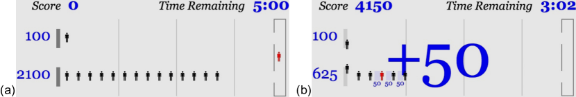
Figure 4: The queue-waiting game. (a) The player (red icon) is in the vestibule, prior to choosing a queue. Queues advance right to left. Points awarded per queue are displayed left of the queue. (b) A snapshot of the game taken while the queues advance. As described in the text, this condition includes bonuses at certain positions in the long queue. Point increments are flashed as they are awarded.

Note that the reward rate (points per action) for either queue does not depend on the long-queue length. Because of this constraint, each episode is functionally decoupled from following episodes. That is, the optimal action for the current episode will not depend on upcoming episodes. Due to this fact and the time-constrained nature of the game, the iterated DGMDP in Figure 1b is appropriate for describing a rational player’s understanding of the game. This DGMDP focuses on reward rate and treats a defection as if the player continues to defect until $\tau$ steps are reached, each step delivering the small reward. The vestibule in Figure 4a corresponds to state 1 in Figure 1b and lower queue position closest to the service desk to state $\tau$. Note the left-to-right reversal of the two Figures, which has often confused the authors of this article.

Experiment 1: Varying Reward Magnitude

Experiment 1 tested reward-rate ratios ($\rho$) 1.25 and 1.50. Figure 5a shows the reward accumulation by individual participants in the two conditions as a function of time within the session. The two dashed black lines represent the reward that would be obtained by deterministically performing the SS or LL action at each tick of the game clock. (Participants are not required to act every tick.) The traces show that some participants had a strong preference for the short queue, others had a nearly perfect preference for the long queue, and still others alternated between strategies. The variability in strategy over time within an individual suggests that they did not simply lock into a fixed, deterministic action sequence.

For each participant, each queue length, and each of the $\tau$ positions in a queue, we compute the fraction of episodes in which the participant defects at the given position. We average these proportions across participants and then compute empirical hazard curves. Figure 5b shows hazard curves for each of the six queue lengths and the two $\rho$ conditions. The $\rho=1.50$ curves are lighter and are offset slightly to the left relative to the $\rho=1.25$ curves to make the pair more discriminable. The Figure presents both human data—asterisks connected by dotted lines—and simulation results—circles connected by solid lines. Focusing on the human data for the moment, initial-defection rates rise slightly with queue length and are greater for $\rho=1.25$ than for $\rho=1.50$. We thus see robust evidence that participants are sensitive to game conditions.

To model the population data, we set the DGMDP parameters ($\Theta_{\text{task}}$) based on the game configuration. We obtain least-squares fits to the four agent parameters ($\Theta_{\text{agent}}$): discount rate $\gamma=0.957$, initial and delta bias spreads $\sigma_{1}=81.3$, and $\sigma=21.3$, and effort cost $\mu_{\textrm{\tiny E}}=-52.1$. The latter three parameters can be interpreted using the scale of the SS reward, $\mu_{\textrm{\tiny SS}}=100$ points. Although the model appears to fit the pattern of data quite well, the model has four parameters and the data can essentially be characterized by four qualitative features: the mean rate of initial defection, the modulation of the initial-defection rate based on queue length and on $\rho$, and the curvature of the hazard function. The model parameters have no direct relationship to these features of the curves, but the model is flexible enough to fit many empirical curves. Consequently, we are cautious in making claims for the model’s validity based solely on the fit to Experiment 1. We note, however, that we investigated a variant of the model in which bias is uncorrelated across steps, and it produces qualitatively the wrong prediction: it yields curves whose hazard probability depends only on the steps to the LL reward. In contrast, the curves of the correlated-bias account depend primarily on the distance from the initial state, $t$, but secondarily on distance to the LL reward, $\tau-t$.

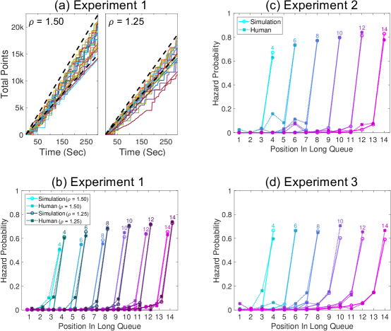
Figure 5: (a) Game points accumulated by individual participants over time in Experiment 1. (b) Hazard curves in Experiment 1 for 6 line lengths and two reward-rate ratios. Human data shown with asterisks and dashed lines, model fits with circles and solid lines. (c) Hazard curves for Experiment 2, with only one free model parameter, (d) Hazard curves for Experiment 3, with no free model parameters.

Experiments 2 and 3: Modulating Effort

To obtain additional support for the theory, we modified the queue-waiting game such that players had to work harder and experienced more frustration in reaching the front of the long queue. By increasing the required effort, we may test whether model parameters fit to Experiment 1 will also fit new data, changing only the effort parameter, $\mu_{\textrm{\tiny E}}$. The long queue’s dynamics were modified to increase the required effort. Instead of advancing deterministically every clock tick as in Experiment 1, the long queue advanced in an apparently random fashion on half the ticks. To move with the queue, the player needed to press the advance key every tick, thus requiring exactly two keystrokes for each action in the game FSM (Figure 1b). The game clock in Experiment 2 updated twice as fast as in Experiment 1 (1000 msec versus 2000 msec); consequently, the overall timing was unchanged. We tested only reward-rate ratio $\rho=1.50$.

Figure 5c shows hazard curves for Experiment 2. Using Experiment 1 parameter settings for $\gamma$, $\sigma_{1}$, and $\sigma$, we fit only the effort parameter, obtaining $\mu_{\textrm{\tiny E}}=-99.7$, which is fortuitously twice the value obtained in Experiment 1. Model fits are superimposed over the human data. To further test the theory’s predictive power, we froze all four parameters and ran an Experiment 3 identical to Experiment 2 except that we introduced a smattering of 50 and 75 point bonuses along the path to the LL (see example in Figure 4b). We also reduced the front-of-queue reward such that the reward-rate ratio $\rho=1.50$ was attained when traversing the entire queue. Using the fully constrained model from Experiment 2, the fit obtained for Experiment 3 was quite good (Figure 5d). The model may slightly underpredict long-queue initial defections, but it captures the curvature of the hazard functions due to the presence of bonuses.

Experiment 4: Customized Bonuses to a Subpopulation

In Experiment 4, we tested the effect of bonuses customized to a subpopulation. To set up this Experiment, we reviewed the Experiment 2 data to examine inter-participant variability. We stratified the 30 participants in Experiment 2 based on their mean reward rate per action. This measure reflects quality of choices and does not penalize individuals who are slow. With a median split, the weak and strong groups have average reward rates of 103 and 132, respectively. Theoretically, rates range from 0 (always switching between lines and never advancing) to 100 (deterministically selecting the short queue) to 150 (deterministically selecting the long queue). We fit the hazard curves of each group to a customized $\gamma$, leaving unchanged the other parameters previously tuned to the population. We obtained excellent fits to the distinctive hazard functions with $\gamma_{\text{strong}}=0.999$ and $\gamma_{\text{weak}}=0.875$.

We then optimized bonuses for each group for various line lengths. As in Figure 3c, we searched over a bonus space consisting of all arrangements of up-to four bonuses, each worth fifty points, allowing multiple bonuses at the same queue position. We subtracted 200 points from the LL reward, maintaining a reward-rate ratio of $\rho=1.50$ for completing the long queue. We constrained the search such that no mid-queue defection strategy would lead to $\rho>1$. A brute-force optimization yields bonuses early in the queue for the weak group, and bonuses late in the queue for the strong group (Figure 6a).

Figure 6: (a) Experiments 4 and 5: Model-predicted optimal bonus sequences, with early (yellow) and late (blue) bonuses for weak and strong participants, respectively. (b) Experiment 4: Average reward rate for weak and strong subpopulations and three bonus conditions. Error bars are $\pm 1$ SEM, corrected for between-subject variance [35]. (c) Experiment 5, Pearson correlation of individual participant’s reward rate and model prediction. The vertical dashed lines indicate the correlation when parameters estimated from an individual’s no-bonus condition performance is used to predict that individual’s bonus-condition performance. The distributions reflect shuffled parameters, i.e., when model parameters fit to one individual are used to predict another individual’s performance.

Experiment 4 tested participants on three line lengths—6, 10, and 14—and three bonus conditions—early, late, and no bonuses. (The no-bonus case was as in Experiment 2.) The 54 participants who completed Experiment 4 were median split into a weak and a strong group based on their reward rate on no-bonus episodes only. Consistent with the model-based optimization, the weak group performs better on early bonuses and the strong group on late bonuses (the yellow and blue bars in Figure 6b). Importantly, there is a $2\times 2$ interaction between group and early versus late bonus ($F(1,51)=11.82$, $p=.001$) indicating a differential effect of bonuses on the two groups. Figure 6b also shows model predictions based the parameterization determined from Experiment 2. The model has a perfect rank correlation with the data, and correctly predicts that both bonus conditions will facilitate performance, despite the objectively equal reward rate in the bonus and no-bonus conditions. That bonuses will improve performance is nontrivial: the persistence induced by the bonuses must overcome the tendency to defect because the LL reward that can be obtained in the bonus condition is reduced to compensate for the bonuses.

Experiment 5: Predicting Individual Bonus Sensitivity

Whereas Experiment 4 customized bonuses to a subpopulation, Experiment 5 focuses on individuals. To avoid the possible confound of intermixing of bonus and no-bonus trials, the experiment was divided into two phases: a four minute phase with no bonuses and a 7 minute phase with the early and late bonus structures used in Experiment 4.

We separately fit the $\Theta_{\text{agent}}$ parameters to the data from each participant in phase 1 and then used the parameterized model to predict average reward rate in the two bonus conditions of phase 2. The model obtains correlations with individuals’ early- and late-bonus reward rates of 0.81 and 0.85, respectively. When parameters fit to one individual are used to predict performance of another randomly drawn individual (shuffled parameters), the median correlation drops to -0.004 and -0.008. The top and middle panels of Figure 6c show the correlation distribution over 10,000 shuffles. The matched-parameter model is clearly an outlier: none of the 10,000 shuffles yields correlations higher than the one we observe for the matched-parameter model. Thus, the parameters inferred from the no-bonus phase are able to predict a specific individual’s response to the presence of bonuses.

A critical test of the theory is whether it can anticipate which bonus structure is superior for an individual. The matched-parameter model obtains a correlation of 0.42 with the reward-rate difference between early and late bonuses, versus a median of 0.005 for shuffled parameters. The model predictions are far better than one would expect without insight into an individual’s decision making processes (Figure 6c, bottom panel): only 30 of 10,000 shuffled parameters yield a correlation as large as the matched-parameter model (i.e., $p=.003$). One should not be disappointed that the model cannot perfectly predict the relative advantage of early versus late bonuses: model-parameter and reward-rate estimates are based on only three minutes of data collection apiece. Consequently, the resulting model predictions and dependent measures are intrinsically noisy which bounds the maximum correlation.

Discussion

In this article, we developed a formal theoretical framework to modeling the dynamics of intertemporal choice. We hypothesized that the theory is suitable to modeling human behavior. We obtained support for the theory by demonstrating that it explains key qualitative behavioral phenomena and predicts quantitative outcomes from a series of behavioral experiments. Although our first experiment merely suggests that the theory has the flexibility to fit behavioral data post hoc, each following experiment used parametric constraints from the earlier experiments, leading to strong predictions from the theory that match behavioral evidence. The theory allows us to design incentive mechanisms that steer individuals toward better outcomes, 3), and we showed that this idea works in practice for customizing bonuses to subpopulations and individuals playing our queue-waiting game. Because the theory has just four free parameters, it is readily pinned down to make strong, make-or-break predictions. Furthermore, it should be feasible to fit the theory to individuals as well as to subpopulations. With such fits comes the potential for maximally effective, truly individualized approaches to guiding intertemporal choice.

The contributions of our work can be appreciated by contrast with the recent work of Lieder et al. [18], which is also aimed at using formal theories of decision making to design incentives. Their incentives take the form of “breadcrumbs” (our term) that reduce the cognitive effort required to attain optimal performance. The approach depends on being able to restructure environments by manufacturing pseudo-rewards that need to be interpreted by participants as if they are actual rewards—often expressed in dollars—but which are not actually paid out. This approach is quite sensible in tasks where individuals procrastinate to avoid effort. However, in a delayed gratification task, this approach is effectively like promising a participant in a retirement plan that they will receive a 65" flat screen TV if they deposit funds in their retirement account and then not actually delivering it. Pseudo-rewards may work in cognitive tasks where participants are seeking breadcrumbs to follow, but unfulfilled promises will quickly lose their appeal in a delayed-gratification task. Another contrast between our work and that of Lieder et al. [18] is our focus on modeling individuals by fitting model parameters using a behavioral assessment and then optimizing incentives to the individual. This exercise places strong demands on the model.

The next step in our research program is to demonstrate utility in incentivizing individuals to persevere toward long-term goals on the time scale of months and years such as losing weight or saving for retirement. It remains uncertain whether intertemporal choice on a long time scale has the same dynamics as on the short time scale of our queue-waiting game. However, our modeling framework is in principle scale invariant, and the finding that reward-seeking behavior on the time scale of eye movements can be related to reward-seeking behavior on the time scale of weeks and months [37, 38] leads us to hope for scale invariance.

Methods

Experimental protocol. The experiments were conducted with informed consent approved by from the University of Colorado’s Institutional Review Board. Participants were recruited using the Amazon Mechanical Turk website and were compensated for their time at the rate of 8$ per hour. Five experiments were conducted all of which were based on the same basic protocol. Subjects were provided instructions to play the ’Queue Waiting game’ in which they controlled the position of a player (in red, Figure 4a). When in the waiting area, subjects could choose to move their player to either a short queue with no waiting time but a reward amount of $100$ points, or a longer queue with varying lengths, $\tau$, but proportionally larger rewards, $100\tau\rho$ points. Each experiment had a fixed duration for which subjects repeatedly performed the queue waiting task. The longer queue had a higher rate if reward, $\rho$, making it the more rewarding choice over the course of the game. The queue lengths, as well as the reward rate of the longer queue proportional to the short queue, were varied in each experiment to test varying aspects of subjects’ behavior.

Bonus presentation. The protocol was designed with the expectation that, to varying degrees, subjects would commit to the longer queue at the beginning and defect to the shorter one before obtaining the larger reward. Therefore, as described in the main text, we designed incentives to help individuals persist with their choice of the longer line. While the theory behind the incentive design has been described earlier, here we describe its appearance in the protocol. Bonus points were systematically placed in selected positions in the queue (Figure 4b) and correspondingly reduced from the final reward, in effect shifting a small portion of the reward earlier in time. Subjects received audio-visual stimuli corresponding to the bonus rewards which changed with the bonus magnitudes as well; the auditory sounds were all variations of a cash register "Ka-Ching" sound.

Data analysis and metrics. In our analyses of player behavior we found that at the start, players are learning the game actions and at the end, players may not have sufficient time to traverse the long queue and defection is the optimal strategy. Therefore, we remove the first and last thirty seconds of play. To measure their behavior we compute an empirical hazard rate (theoretically defined as in Equation (4)); for each participant, each queue length, and each of the $\tau$ positions in a queue, we compute the fraction of episodes in which the participant defects at the given position. We average these proportions across participants and then compute empirical hazard rate per line position per subject. When visualizing the theoretical or empirical hazard rates with respect to line position, we are able to generate hazard curves, using which we can determine how well the model fits empirical data as in Figure 5b—d.

Across all the experiments, participants are paid at a rate of $8.00 per hour and are awarded a score-based bonus. If they fail to act, they are warned after 7 idle seconds and rejected after 14 seconds. They are also rejected if they de-focus their browser twice, with a warning message after the first time. Specifics regarding the protocol are described for each experiment below.

In each experiment, the first thirty seconds of game play are discarded to allow participants to figure out the game, and the last thirty seconds are discarded due to the possibility of greedy end-of-game strategies. In Experiment 5, the last 30 seconds of phase 1 game play are also discarded.

Experiment 1: In this experiment, two values of the reward rate ratio, $\rho\in\{1.25,1.50\}$, were tested to determine participants’ sensitivity to the conditions of the game. Six lengths were tested across multiple iterative episodes for the long queue uniformly drawn from $\{4,6,8,10,12,14\}$. At each update of the game state which happened every 2 seconds, both queues advanced. The player advanced along with the queues if subjects pressed the left arrow key just before the game state updated. Both queues advanced deterministically on each update. Forty-one participants were recruited, twenty for the $\rho=1.50$ condition and twenty-one for the $\rho=1.25$ condition.

To compare the empirical data on participants’ behavior to the model’s predictions, we simulated the model by setting the task parameters $\Theta_{task}$ in our DGMDP based on our game configuration and obtained least squares fits for the parameters that determine subjective behvaiour $\Theta_{agent}$, namely the discount rate $\gamma$, the spread in bias distribution $\sigma$ as well as the initial value at the first time step $\sigma_{1}$, and effort cost $\mu_{\textrm{\tiny E}}$.

Experiment 2: For this experiment, moving the player through the line was made more effortful. The game state was updated every second, twice as fast as in experiment 1. However, to move the player through the queue, while every game state update required a key stroke, only one would result in a movement requiring two keystrokes per action. Therefore, advancing one position in the queues required two keystrokes as opposed to one, with the longer queue advancing pseudorandomly ensuring that an equal number of advances got the player to the end of the queue. The same set of lengths for the long queue as in experiment 1 was experienced by participants in experiment 2. Only one reward rate ratio $\rho=1.50$ was tested in this experiment and thirty participants were recruited to perform the task.

The effort parameter from the model $\mu_{\textrm{\tiny E}}$ was obtained by fitting the model to the data while using the fits for the other parameters as determined from experiment 1 ($\gamma$,$\sigma$,$\sigma_{1}$).

Experiment 3: This experiment was run to test the predictive power of a fully-constrained model from experiment 2 on unseen data. Further, we added small bonus rewards for making it to certain positions (worth 50 or 75 points) in the long queue which were correspondingly subtracted from the final reward in the queue to maintain the reward rate ratio of $\rho=1.50$ if the entire queue was traversed. The fully constrained model’s hazard rates were compared with empirical performance for the population in this experiment with the game parameters (bonuses and final reward) adjusted accordingly. Length of the longer queue was sampled from the same set of six lengths as in the previous two experiments. Thirty participants were recruited for this task.

Experiment 4: This experiment was designed to determine the effects of customized bonuses to sub-populations. Bonus schemes were designed based on data from experiment 2 within which subjects’ performance was stratified and categorized into two groups—strong and weak groups based on their earned average reward. Models were fit to the two groups separately and bonuses were then optimized to improve performance based on simulations for the two sub-populations. Bonuses awarded were subtracted from the final reward as in experiment 3 to maintain the reward rate. Brute force optimization yielded a strategy that provided early bonuses for the weak group and late bonuses to the strong group. In this experiment, three lengths were used for the longer queue, $\tau\in\{6,10,14\}$. The three queues were presented in three conditions—the no bonus, early bonus and late bonus conditions. Fifty-four participants were recruited to perform this experiment. When analyzing the data subjects were similarly grouped into strong and weak categories based on a median-split on their empirical reward rate in the no-bonus condition. Their performances in the early and late bonus conditions were then compared using a two-way repeated measures ANOVA to test the model’s hypothesis for the sub-populations’ performance on the two bonus conditions.

Experiment 5: The final experiment was designed to determine if the model could predict performance of individuals in specified bonus conditions. The experiment had two phases, the first being a no bonus phase followed by a bonus phase with both early and late bonuses. Lengths used for the longer queue were the same as in experiment 4. Forty subjects were tested in this experiment, but data from one had to be excluded given abnormally long date update times indicating a problem with the game run on their end. The no bonus phase was four minutes long while the bonus phase was seven minutes long. The game state was updated every second.

For each individual participant, the DGMDP was fit to their no bonus phase to determine each individual set of parameters $\Theta_{agent}$. Based on the fit parameters per individual, their performance in the early and late bonus phase was predicted and compared to their empirical performance. To determine the efficacy of the fit, each individual participant’s fitted model was used to predict performance of of another randomly selected subject to ensure that predictions were not just random. For each bonus type, early and late, predicted and actual performance was compared within subject along with 250 shuffled pair comparisons to ensure performance was above random chance. Further, to ensure that the model was not just scaling performance of good or bad subjects in the bonus conditions, we also determined how good it was in determining the difference between each individual’s performance in the early versus the late bonus conditions. Once again, the predicted and actual data pairs were shuffled 250 times to compare performance to random chance.

Acknowledgments

This research was supported by NSF grants DRL-1631428, SES-1461535, SMA-1041755, and seed summer funding from the Institute of Cognitive Science at the University of Colorado. We thank John Lynch for initial discussions that led to this collaboration, Ian Smith and Brett Israelson for assistance in the design and coding of experiments, and Pradeep Shenoy and Doug Eck for helpful comments on an earlier draft of the manuscript.

Supplementary Information

Modelling

Bias

Critical to our model is the random walk in bias, $w$ (Equation 1 in the main article). As we stated in the main article, it is essential for the model predictions that $w$ has temporal autocorrelations. Ideally, we might have selected pink ($1/f$) noise rather than brown (Gaussian) noise for its scale invariant property. Our model should be capable of explaining behavior in tasks where defections happen on the time scale of seconds (e.g., the line-waiting game) to years (e.g., retirement planning); scale invariant pink noise facilitates such scale invariance. However, the Gaussian formulation is mathematically convenient and facilitates simulations and our approximations.

Depending on the time scale, the bias might conceivably reflect fluctuations in life stress, sleep deprivation, mood, hunger, or cognitive load. However, we resist attaching an association between $w$ and these cognitive factors, as evidence suggests that factors such as hunger affect delay discounting [e.g., 39]. We also resist considering $w$ to relate directly to willpower, resolve, impulsivity, or grit: we argue that these psychological constructs emerge from the operation of a complex decision-making system rather than being primitive mechanisms like the fluctuations in $w$. Also, these constructs operate on a much slower time scale than the second-to-second fluctuations we model in our line-waiting experiment and impulsivity and grit are considered enduring personality traits not a time-varying state [40].

We rejected several alternative forms of noise.

1. An obvious possibility, mentioned previously, is treating the discounting rate as a random variable. However, our goal is to propose a model that could be considered scale invariant, and it seems cognitively implausible that discount rates fluctuate significantly on a second-by-second basis, considering that they are often used as a stable biomarker of individual differences [41].

2. We also decided against using $w$ as a multiplicative modulation, partly because the additive form is more amenable to analyses of the model, and partly because doing so would predict insensitivity to scaling of SS and LL rewards.

3. Our modeling and prediction was over a time period of minutes. Over long time periods, it may be necessary to consider a mean-reverting diffusion process that causes $w$ to decay back to zero in the absence of noise perturbations. We omitted decay simply to avoid an additional parameter of the model, i.e., essentially fixing a decay rate of 0.

For the purpose of our model, the critical decision for $w$ is that it is a random process that cannot be directly manipulated by executive control processes.

Approximating the Value Function

Consider the shape of $V(t,w)$. With high bias ($w\to\infty$), the agent almost certainly persists to the LL reward and the function asymptotes at the discounted $\mu_{\textrm{\tiny LL}}$. With low bias ($w\to-\infty$), the agent almost certainly defects and the function approaches $\mu_{\textrm{\tiny SS}}-w$. Thus, both extrema of the value function are linear with known slope and intercept. At step $\tau$, these two linear segments exactly define the value function. At $t<\tau$, there is an intermediate range within which small fluctuations in bias can influence the decision and the expectation in Equation 2 of the main article yields a weighted mixture of the two extrema, which is well fit by a single linear segment—defined by its slope $a_{t}$ and intercept $b_{t}$. With $V(t,w)$ expressed as a piecewise-linear approximation, the expectation in Equation 2 of the main article becomes:

$$\begin{split}\mathbb{E}_{W_{t}|W_{t-1}=w}V(t,w_{t})=&\Phi\left(z_{t}^{-}\right)(\mu_{\textrm{\tiny SS}}-w)+\left(\Phi\left(z_{t}^{+}\right)-\Phi\left(z_{t}^{-}\right)\right)(b_{t}+a_{t}w)\\ &~{}~{}~{}~{}~{}~{}~{}+\left(1-\Phi\left(z_{t}^{+}\right)\right)c_{t}+\sigma\phi(z_{t}^{-})+\sigma a_{t}\left(\phi(z_{t}^{-})-\phi(z_{t}^{+})\right),\end{split}$$ (6)

where $\Phi(.)$ and $\phi(.)$ are the cdf and pdf of a standard normal distribution, respectively, and the standardized segment boundaries are $z_{t}^{-}=\sigma^{-1}[(\mu_{\textrm{\tiny SS}}-b_{t})/(a_{t}+1)-w]$ and $z_{t}^{+}~{}=~{}\sigma^{-1}[(c_{t}-b_{t})/a_{t}-w]$. The backup is seeded with $z_{\tau}^{-}=z_{\tau}^{+}=\sigma^{-1}(\mu_{\textrm{\tiny SS}}-\mu_{\textrm{\tiny LL}}-w)$ and $a_{\tau}=b_{\tau}=c_{\tau}=\mu_{\textrm{\tiny LL}}$. After each backup step, a Levenberg-Marquardt nonlinear least squares fit obtains $a_{t-1}$ and $b_{t-1}$; $c_{t-1}$—the value of steadfast persistence—is obtained by propagating the discounted reward for persistence: $c_{t-1}~{}=~{}\mu_{\textrm{\tiny E}}+\mu_{t}+\gamma c_{t}$.

To ensure accuracy of the estimate and to eliminate an accumulation of estimation errors, we have also used a fine piecewise constant approximation in the intermediate region, yet the model output is almost identical.

Posterior Estimation of Bias

To represent the posterior distribution over bias at each non-defection step in Equation 4, we initially used particle filters but found a computationally more efficient and stable solution with quantile-based samples. We approximate the $W_{1}$ prior and $\Delta W$ with discrete, equal probability $q$-quantiles. We reject values for which defection occurs, and then propagate $W_{t+1}=W_{t}+\Delta W$ which results in up to $q^{2}$ samples, which we thin back to $q$-quantiles at each step. Using $q=1000$ produces nearly identical results to selecting a much higher density of samples.

Conditions of Equivalence of One-Shot and Iterative Delayed-Gratification Tasks

The one-shot DGMDP in Figure 1a of the main article can be extended to model the iterated task, shown in Figure 1a, even when there is variability in the reward ($\mu_{\textrm{\tiny LL}}$) or duration ($\tau$) across episodes, shown in Figure 1b. Figures 1a,b describe an indefinite series of episodes. If the total number of episodes or steps is constrained, as in any realistic scenario (e.g., an individual has eight hours in the work day to perform tasks like answering email), then the state must be augmented with a representation of remaining time. We dodge this complication by modeling situations in which the ‘end game’ is not approaching, e.g., only the first half of a work day.

It is straightforward to show that the solution to the iterated DGMDP in Figure 1b is identical to the solution to the simpler and more tractable one-shot DGMDP in Figure 1b of the main article under certain constraints that we describe next. These constraints ensure that there is no interdependence among episodes, allowing a one-shot DGMDP (Figure 1b) to serve as a proxy for an iterative task (Figure 1b).

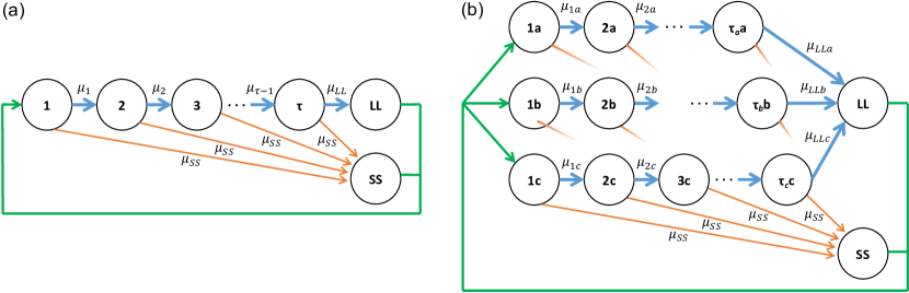
Figure 1: Finite-state environment formalizing (a) the iterated delayed-gratification task; (b) the iterated delayed-gratification task with variable delays and LL outcomes

Consider the value function for a special case where the bias does not fluctuate, i.e., $\sigma^{2}=0$ and where intermediate rewards are not provided, i.e., $\mu_{i}=0$ for $i\in\{1...\tau-1\}$. In this case, we can show that the solution to the DGMDP in Figure 1b is identical to the solution to the DGMDP in Figure 1b of the main article.

We need to extend this result to the following more general cases, roughly in order of challenge:

• Allow for nonzero intermediate rewards

• Allow for the case of Figure 1b where $\mu_{\textrm{\tiny LLa}}/\tau_{a}=\mu_{\textrm{\tiny LLb}}/\tau_{b}$ for all $a$ and $b$,

• Allow for the case where $\sigma^{2}>0$

Proof of $\sigma^{2}=0$ and $\mu_{i}=0$ case

In Figure 1a, the value of state 1 is defined by the Bellman equation as:

$$V(1)=\max(\mu_{\textrm{\tiny SS}}+\gamma V(1),\gamma^{\tau-1}[\mu_{\textrm{\tiny LL}}+\gamma V(1)])$$ (7)

We can solve for $V(1)$ if the first term is larger:

$$V_{\mathrm{SS}}(1)=\frac{1}{1-\gamma}\mu_{\textrm{\tiny SS}}.$$ (8)

We can solve for $V(1)$ if the second term is larger:

$$V_{\mathrm{LL}}(1)=\frac{\gamma^{\tau-1}}{1-\gamma^{\tau}}\mu_{\textrm{\tiny LL}}.$$ (9)

Now consider Figure 1b of the main article, whose Bellman equation can be simplified to:

$$V(1) =\max\left(\sum_{i=0}^{\tau-1}\gamma^{i}\mu_{\textrm{\tiny SS}},\gamma^{\tau-1}\mu_{\textrm{\tiny LL}}\right)$$ (10)

$$=\max\left(\frac{1-\gamma^{\tau}}{1-\gamma}\mu_{\textrm{\tiny SS}},\gamma^{\tau-1}\mu_{\textrm{\tiny LL}}\right)$$ (11)

$$=(1-\gamma^{\tau})\max\left(\frac{1}{1-\gamma}\mu_{\textrm{\tiny SS}},\frac{\gamma^{\tau-1}}{1-\gamma^{\tau}}\mu_{\textrm{\tiny LL}}\right).$$ (12)

Note that the two terms inside the max function of Equation 12 are identical to the values in Equations 8 and 9, and thus the value functions for Figure 1b of the main article and Figure 1b are identical up to a scaling constant.

Hyperbolic discounting

One challenge to modeling behavior with MDPs is that it is mathematically convenient to assume exponential discounting, whereas studies of human intertemporal choice support hyperbolic discounting [42]. Kurth-Nelson and Redish [26] have proposed a solution to this issue by exploiting the fact that a hyperbolic function can be well approximated by a mixture of exponentials. In our models, we found that exponential discounting was adequate to explain behavior, but our approach could readily be extended in the same manner as Kurth-Nelson and Redish [26]. With a mixture of exponential discounting rates [43, 44], it becomes feasible to model individual moment-to-moment variability as fluctuations in the discount rate, which correspond to different weightings of the exponential decays.

Simulation details

In simulations, we assume the effort cost $\mu_{\textrm{\tiny E}}=0$ on steps when the player is served the front-of-line reward. Similarly, we assume that $\mu_{\textrm{\tiny E}}=0$ on any step leading to a bonus.

Experiment 5

In Experiment 5, we obtained parameters $\Theta_{\text{agent}}$ for each individual based on their behavior in phase 1. We then predicted individuals’ reward rate on the early and late bonus trials in phase 2. The scatterplot of predicted and actual reward rates is shown in Figure 2a,b for early and late bonuses. Figure 2c shows the correlation of the difference between late and early rates. To evaluate the degree to which these parameters characterize an individual’s behavior, we shuffled the assignment of parameters to individuals.

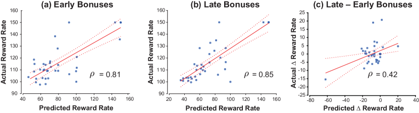
Figure 2: Experiment 5, comparing predicted and observed reward rates. The predicted reward rate for each individual is estimated via model simulations with model parameters fit to the individual’s no-bonus phase data. (a) Early-bonus condition scatterplot, with regression line and confidence interval. (b) Late-bonus condition scatterplot. (c) Difference between reward rates for early versus late bonus conditions.

Experiment Instruction Phase

Before each experiment began, subjects were given instructions and shown corresponding examples of the game screen. In each experiment, they were instructed that their goal was to reach the front of the queue to score the points indicated to the left of each queue, and that they controlled the stick figure in red (Fig 3(a)). Following this they were given instructions to choose the top or bottom queue by either pressing the up or down arrow key when the player was in the waiting area (Fig 3(b)). Once out of the waiting area, subjects were told that they could advance their player by hitting the ‘Left’ arrow key; they could defect between lines using the up or down arrow key. Finally, once they reached the front of the queue, they earned the corresponding reward which set the player back to the waiting area (Fig 3(c)). In experiments 1–4, they were instructed that this task would be repeated for 5 minutes. In experiments 3 and 4, subjects also had the opportunity to earn bonuses for crossing certain spots in the larger cue (Fig 3(d)). Once they passed that spot, they received audiovisual confirmation for earning the bonus reward.

In experiment 5, subjects were informed that, after the control phase of 4 minutes, they will receive further instructions to perform the remainder of the task with the total task lasting 11 minutes. At the break between the tasks, they were informed that for the next 7 minutes they would also earn bonuses at certain spots (Fig (Fig 3(d))) in the long line. In all experiments, they were informed that they had to keep playing to keep the experiment from being aborted.

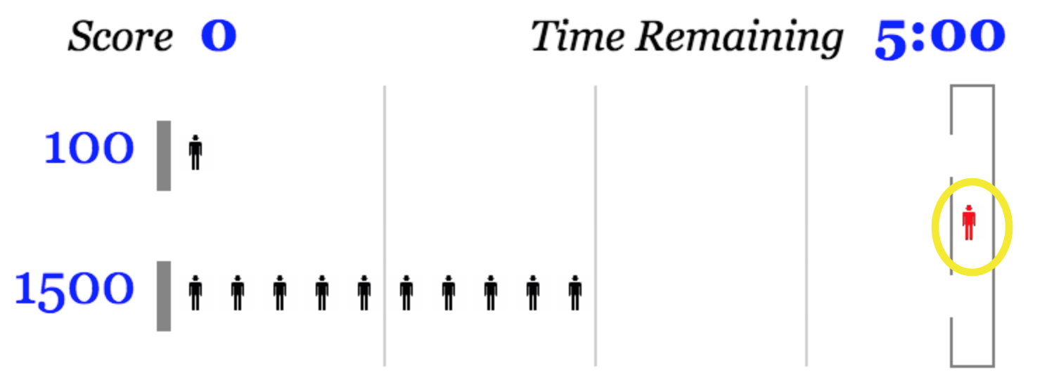
(a)

(b)

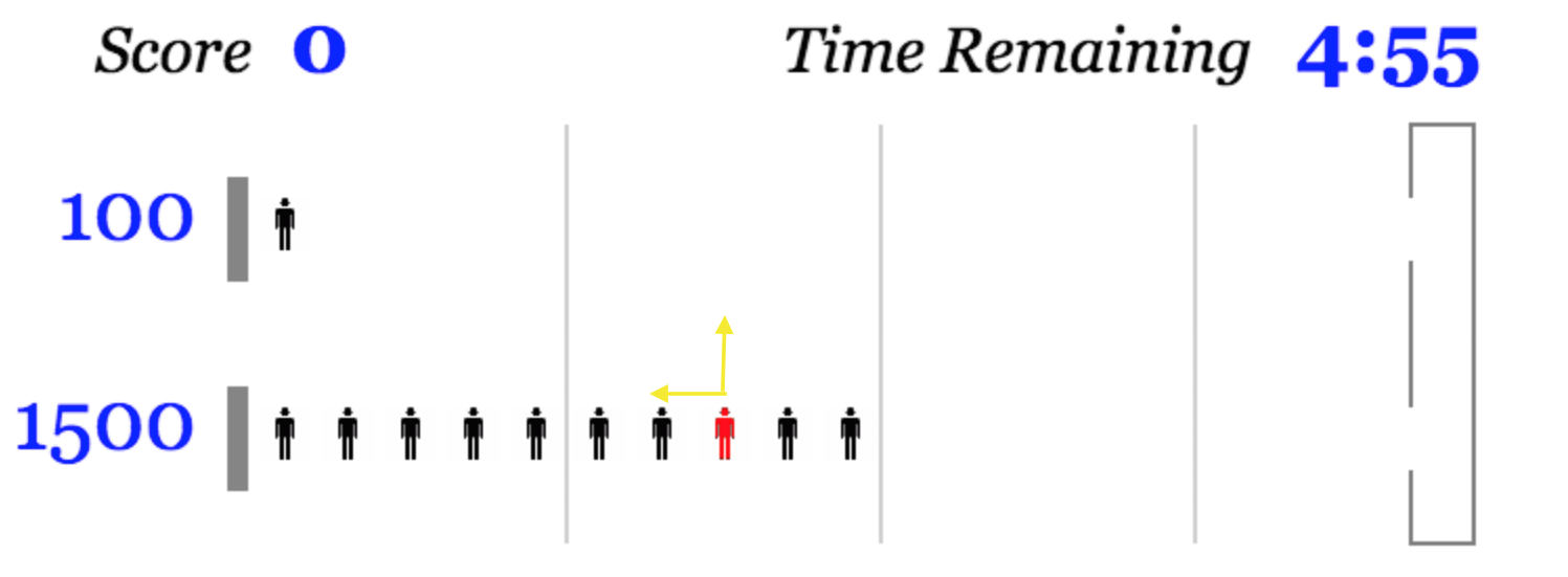
(c)

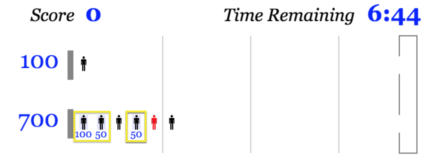
(d)

Figure 3: Subjects were shown examples of the game screen with annotated instructions: (a) They were instructed to move their player, indicated in red to the front of the queue. (b) The up or down arrow key could be used to select the line they wanted to move trhough.(c) Subjects can advance through the queue using the left arrow key and free to switch between lines using the up or down arrow key. Once they reached the end of the queue they earned the points indicated to the left of the queues. (d) Subjects also were able to earn bonuses at certain spots in the queue as indicated under the spot.

Comment on related research

Lieder et al. [18] use the MDP framework to propose incentive structures in which the one-step greedy action is also the long-term optimal action. In their Experiments 1 and 2, participants are given explicit instructions to follow the “breadcrumbs” (our term) provided by the incentive structure to attain optimal performance, thereby eliminating the cognitive effort required to choose the optimal action. In their Experiments 3 and 4, the approach gives direct guidance about what action participants should take next to make the most progress to a large payoff. In all their experiments, the more explicit the breadcrumbs are, the more effectively they are followed. For instance, in Experiment 4, the optimal incentives have positive and negative dollar values for choices an individual should prioritize and deprioritize, respectively (colored red and green, no less). In contrast, an alternative heuristic incentive condition provides all positive dollar values (all colored green), which demands inspecting and sorting the relative magnitudes of the dollar values. The approach depends on being able to restructure environments by manufacturing pseudo-rewards that need to be interpreted by participants as if they are actual rewards—often expressed in dollars—but which are not actually paid out.

To contrast our work with that of Lieder et al. [18]:

• We study canonical delayed gratification task that requires patience, whereas the laboratory tasks of Lieder et al. encourage procrastination or short cuts to avoid effort.

• We have shown that our model fits human behavioral data directly, rather than the indirect evidence that Lieder et al. obtain by using their model to determine pseudo-rewards. To fit behavioral data, it is necessary to make assumptions beyond those in the standard MDP framework in order to explain variability in individual behavior.

• We customize our model to individuals (or subpopulations) through the observation of baseline behavior and maximum-likelihood model-parameter fits. In contrast, Lieder et al. [18] assume fixed parameters (e.g., discount factor, goal-abandonment probability) for all individuals.

• The bonuses we provide to participants are expressed in the same currency as outcomes and are actually awarded, and our bonus scheme is constrained such that the reward rate obtained by harvesting bonuses cannot exceed that obtained with no bonuses. Further, our bonus computation ensures consistency in currency between the bonuses and the long term rewards. This structure can therefore be easily adopted to real-world tasks with food and monetary rewards. In contrast, fabricated pseudo-rewards are unbounded and have questionable subjective value in many scenarios. For example, if everyone is awarded 1000 stars, what value does a star have?

• Our emphasis has been optimizing incentives for an individual, and we have done the strong contrast to show that incentives optimized for one individual are more effective than those optimized for another.

References

- [1]
- Rhee and Boivie [2015] Rhee, N., & Boivie, I. (2015). The continuing retirement savings crisis. Tech. rep., National Institute on Retirement Security.
- Goodman et al. [2021] Goodman, L., Mortenson, J., Mackie, K., & Schramm, H. R. (2021). Leakage from retirement savings accounts in the United States. National Tax Journal, 73, 689–719.
- Fernandes et al. [2014] Fernandes, D., Lynch, J. G., Jr., & Netemeyer, R. G. (2014). Financial literacy, financial education, and downstream financial behaviors. Management Science, 60, 1861–1883.
- Kearney et al. [2010] Kearney, M. S., Tufano, P., Guryan, J., & Hurst, E. (2010). Making savers winners: An overview of prize-linked savings products. Working Paper 16433, National Bureau of Economic Research.
- Gertler et al. [2019] Gertler, P., Higgins, S., Scott, A., & Seira, E. (2019). Increasing financial inclusion and attracting deposits through prize-linked savings. Unpublished manuscript, University of California, Berkeley, and Instituto Tecnológico Autónomo de México. https://seankhiggins. com/assets/pdf/GertlerHigginsScottSeira_PrizeLinkedSavings.pdf.
- Kahneman and Tversky [1979] Kahneman, D., & Tversky, A. (1979). Prospect theory: An analysis of decision under risk. Econometrica, 47, 263–292.
- Green and Myerson [2004] Green, L., & Myerson, J. (2004). A discounting framework for choice with delayed and probabilistic rewards. Psychological Bulletin, 130, 769–792.
- Kirby [2009] Kirby, K. N. (2009). One-year temporal stability of delay-discount rates. Psychological Bulletin & Review, 16, 457–462.
- Mischel and Ebbesen [1970] Mischel, W., & Ebbesen, E. B. (1970). Attention in delay of gratification. Journal of Personality and Social Psychology, 16, 329–337.
- Ainslie [2021] Ainslie, G. (2021). Willpower with and without effort. Behavioral & Brain Sciences.
- Mischel et al. [1989] Mischel, W., Shoda, Y., & Rodriguez, M. (1989). Delay of gratification in children. Science, 244(4907), 933–938.
- McGuire and Kable [2013] McGuire, J. T., & Kable, J. W. (2013). Rational temporal predictions can underlie apparent failure to delay gratification. Psychological Review, 120, 395–410.
- Niv et al. [2007] Niv, Y., Daw, N. D., Joel, D., & Dayan, P. (2007). Tonic dopamine: opportunity costs and the control of response vigor. Psychopharmacology, 191(3), 507–520.
- Niv et al. [2012] Niv, Y., Edlund, J., Dayan, P., & O’Doherty, J. (2012). Neural prediction errors reveal a risk-sensitive reinforcement-learning process in the human brain. The Journal of Neuroscience, 32, 551–562.
- Shen et al. [2014] Shen, Y., Tobia, M. J., Sommer, T., & Obermayer, K. (2014). Risk sensitive reinforcement learning. Neural Computation, 26, 1298–1328.
- Lieder et al. [2019a] Lieder, F., Callaway, F., Jain, Y. R., Krueger, P. M., Das, P., Gul, S., & Griffiths, T. (2019a). A cognitive tutor for helping people overcome present bias. In C. Hartley, & M. Littman (Eds.) Proceedings of Reinforcement Learning and Decision Making, (pp. 292–296).
- Lieder et al. [2019b] Lieder, F., Chen, O. X., Krueger, P. M., & Griffiths, T. (2019b). Cognitive prostheses for goal achievement. Nature Human Behavior, 3, 1096–1106.
- Drummond and Niv [2020] Drummond, N., & Niv, Y. (2020). Model-based decision making and model-free learning. Current Biology, (pp. PR860–R865).
- Widrich et al. [2021] Widrich, M., Hofmarcher, M., Patil, V., Bitto-Nemling, A., & Hochreiter, S. (2021). Assigning credit to human decisions using modern Hopfield networks. In D. Reichman, J. Peterson, K. Tomlinson, A. Liang, & T. L. Griffiths (Eds.) Proceedings of the 2021 Workshop on Human and Machine Decision Making. San Diego, CA: Neural Information Processing Systems Foundation.
- Bastani et al. [2021] Bastani, H., Bastani, O., & Sinchairsi, P. (2021). Improving human decision making with machine learning. In D. Reichman, J. Peterson, K. Tomlinson, A. Liang, & T. L. Griffiths (Eds.) Proceedings of the 2021 Workshop on Human and Machine Decision Making. San Diego, CA: Neural Information Processing Systems Foundation.
- Sutton and Barto [2018] Sutton, R. S., & Barto, A. G. (2018). Reinforcement Learning: An Introduction (2nd Edition). MIT Press.
- Simon [1997] Simon, H. A. (1997). Models of bounded rationality: Empirically grounded economic reason, vol. 3. Cambridge, MA: MIT press.
- Todd and Gigerenzer [2012] Todd, P. M., & Gigerenzer, G. (2012). Ecological Rationality: Intelligence in the World. Oxford U. Press.
- Chater and Oaksford [1999] Chater, N., & Oaksford, M. (1999). Ten years of the rational analysis of cognition. Trends in Cognitive Science, 3, 57–65.
- Kurth-Nelson and Redish [2010] Kurth-Nelson, Z., & Redish, A. D. (2010). A reinforcement learning model of precommitment in decision making. Frontiers in Behavioral Neuroscience, 4.
- Kurth-Nelson and Redish [2012] Kurth-Nelson, Z., & Redish, A. D. (2012). Don’t let me do that! models of precommitment. Frontiers in Neuroscience, 6.
- Mischel et al. [1988] Mischel, W., Shoda, Y., & Peake, P. K. (1988). The nature of adolescent competencies predicted by preschool delay of gratification. Journal of Personality & Social Psychology, 54, 687–696.
- Kivetz [2003] Kivetz, R. (2003). The effects of effort and intrinsic motivation on risky choice. Marketing Science, 22, 477–502.
- Shenhav et al. [2017] Shenhav, A., Musslick, S., Lieder, F., Kool, W., Griffiths, T. L., Cohen, J. D., & Botvinick, M. M. (2017). Toward a rational and mechanistic account of mental effort. Annual Review of Neuroscience, 40, 99–124.
- Mischel [1974] Mischel, W. (1974). Processes in delay of gratification. Advances in Experimental Social Psychology, 7, 249–292.
- Kidd et al. [2012] Kidd, C., Palmeri, H., & Aslin, R. N. (2012). Rational snacking: Young children’s decision-making on the marshmallow task is moderated by beliefs about environmental reliability. Cognition, 126, 109–114.
- Nisan and Ronen [1999] Nisan, N., & Ronen, A. (1999). Algorithmic mechanism design (extended abstract). In Proceedings of the Thirty-first Annual ACM Symposium on Theory of Computing, STOC ’99, (pp. 129–140). New York, NY, USA: ACM.
- Tversky and Kahneman [1992] Tversky, A., & Kahneman, D. (1992). Advances in prospect theory: Cumulative representation of uncertainty. Journal of Risk and Uncertainty, 5, 279–323.
- Masson and Loftus [2003] Masson, M. E., & Loftus, G. R. (2003). Using confidence intervals for graphically based data interpretation. Canadian Journal of Experimental Psychology, 57(3), 203—220.
- Woolley and Fishbach [2016] Woolley, K., & Fishbach, A. (2016). For the fun of it: Harnessing immediate rewards to increase persistence on long-term goals. Journal of Consumer Research, 42, 952–966.
- Shadmehr et al. [2010] Shadmehr, R., de Xivry, J. J. O., Xu-Wilson, M., & Shih, T.-Y. (2010). Temporal discounting of reward and the cost of time in motor control. Journal of Neuroscience, 30(31), 10507–10516.
- Wolpert and Landy [2012] Wolpert, D. M., & Landy, M. S. (2012). Motor control is decision making. Current Opinions in Neurobiology, 22, 996–1003.
- Skrynka and Vincent [2019] Skrynka, J., & Vincent, B. T. (2019). Hunger increases delay discounting of food and non-food rewards. Psychonomic Bulletin & Review, 26, 1729––1737.
- Duckworth et al. [2007] Duckworth, A., Peterson, C., Matthews, M., & Kelly, D. (2007). Grit: Perseverance and passion for long-term goals. Journal of Personality and Social Psychology, 92, 1087–1101.
- Montague et al. [2012] Montague, P. R., Dolan, R. J., Friston, K. J., & Dayan, P. (2012). Computational psychiatry. Trends in Cognitive Science, 16, 72–80.
- Frederick et al. [2002] Frederick, S., Loewenstein, G., & O’Donoghue, T. (2002). Time discounting and time preference: A critical review. Journal of Economic Literature, 40(2), 351–401.
- Tiganj et al. [2017] Tiganj, Z., Shankar, K. H., & Howard, M. W. (2017). Scale invariant value computation for reinforcement learning in continuous time. In AAAI Spring Symposium Series – Science of Intelligence: Computational Principles of Natural and Artificial Intelligence. AAAI Press.
- Fedus et al. [2019] Fedus, W., Gelada, C., Bengio, Y., Bellemare, M. G., & Larochelle, H. (2019). Hyperbolic discounting and learning over multiple horizons. arXiv preprint arXiv:1902.06865.