An efficient multi-modes Monte Carlo homogenization method for random materials

Abstract

In this paper, we propose and analyze a new stochastic homogenization method for diffusion equations with random and fast oscillatory coefficients. In the proposed method, the homogenized solutions are sought through a two-stage procedure. In the first stage, the original oscillatory diffusion equation is approximated, for each fixed random sample $\omega$, by a spatially homogenized diffusion equation with piecewise constant coefficients, resulting in a random diffusion equation. In the second stage, the resulting random diffusion equation is approximated and computed by using an efficient multi-modes Monte Carlo method which only requires to solve a diffusion equation with a constant diffusion coefficient and a random right-hand side. The main advantage of the proposed method is that it separates the computational difficulty caused by the spatial fast oscillation of the solution and that caused by the randomness of the solution, so they can be overcome separately using different strategies. The convergence of the solution of the spatially homogenized equation (from the first stage) to the solution of the original random diffusion equation is established and the optimal rate of convergence is also obtained for the proposed multi-modes Monte Carlo method. Numerical experiments on some benchmark test problems for random composite materials are also presented to gauge the efficiency and accuracy of the proposed two-stage stochastic homogenization method.

65M12, 74Q05

1 Introduction

This paper is concerned with numerical solutions of the following diffusion equation with random coefficients and data encountered in materials science:

(1a) $$-\hbox{div}\Bigl{(}A\biggl{(}\frac{x}{\varepsilon},\omega\biggr{)}\nabla u^{\varepsilon}(x,\omega)\Bigr{)} =f(x,\omega) \qquad\mbox{in }{D}\times\Omega,$$

(1b) $$u^{\varepsilon}(x,\omega) =0 \qquad\mbox{on }\partial{D}\times\Omega.$$

Here ${D}\subset\mathbb{R}^{d}(d=1,2,3)$ is a bounded domain and $\omega$ denotes a sample point which belongs to a probability (sample) space $(\Omega,\mathcal{F},\mathbb{P})$. The coefficient matrix $A(\frac{x}{\varepsilon},\omega)=(a_{ij}(\frac{x}{\varepsilon},\omega))_{1\leq i,j\leq d}$ and the right hand side term $f(x,\omega)$ are random fields with continuous and bounded covariance functions. The parameter $\varepsilon$ represents the size of microstructure for the composite materials, which is usually very small, that is, $0<\varepsilon\ll 1$.

The random diffusion equation (1) has many applications in mechanics, hydrology and thermics (see [15, 19, 24, 26]). A direct accurate numerical solution of (1) is difficult to obtain because it requires a very fine mesh and large-scale sampling of $\omega$, and thus a prohibitive amount of computation time. In the case of absence of the randomness (i.e., the dependence on $\omega$ in (1) is dropped ), the homogenization method has been successfully developed for solving the diffusion equation with periodic deterministic coefficients (cf. [5, 8, 25]), in which the homogenized coefficients are obtained by solving a cell problem defined in the unit cell. For the diffusion equation (1) with random coefficients, a stochastic homogenization theory has also been well developed, see [6, 7, 10, 9, 14, 18, 17, 21, 23, 27, 30]. Similar to the deterministic case, the homogenized diffusion equation is constructed by solving a certain cell problem. However, a fundamental difference is that the stochastic cell problem is a random second order elliptic problem, which is posed in the whole space $\mathbb{R}^{d}$ (see (7)). Solving such an infinite domain problem numerically is not only challenging but also very expensive, and the homogenization methods quoted above did not give any practical recipe for numerically approximating the cell problem and the homogenized equation.

To circumvent the above difficulties, some localized approximations of the effective (or homogenized) coefficients by using “periodization” and “cut-off” procedures were introduced in [2, 7, 22, 31]. A big benefit of the localized approximations is that the resulting cell problem is now posed on a bounded domain and it was proved that the approximated coefficients converge to the effective (or homogenized) coefficients as the size of the bounded domain goes to infinity. We also note that the localized approximation methods, such as the representative volume element (RVE) method, have also been used to compute the effective parameters of highly heterogeneous materials and to calculate the effective coefficients related to random composite materials, by utilizing a possibly large number of realizations [9, 13, 18, 29]. After having constructed the approximated effective (or homogenized) coefficients, the main task then reduces to solve the approximated (random) diffusion equation with the constructed coefficients. As a direct application of Monte Carlo or stochastic Galerkin method, since solving this random diffusion equation is computationally expensive, other more efficient methods have been developed for the job. In [3, 4], a perturbative model for weakly random materials was proposed and the first-order and second-order asymptotic expansions were established by means of an ergodic approximation based on the weak randomness assumption. In [11], a multi-modes Monte Carlo (MMC) finite element method was proposed to solve random partial differential equations (PDEs) under the assumption that the medias (or coefficients) are weakly random in the sense that they can be expressed as small random perturbations of a deterministic background. However, to the best of our knowledge, there is still no efficient method for solving the homogenized equation for problem (1) in general setting.

The goal of this paper is to develop and analyze an efficient and practical two-stage homogenization method for problem (1). In the first stage, we construct a piecewise homogeneous (i.e., piecewise constant) material as an approximation to the original composite material for each fixed sample $\omega$ by solving several cell functions on bounded domains. Under the stationary (process) assumption, we are able to prove that the coefficient matrix of the piecewise homogeneous material can be rewritten as a small random perturbation of a deterministic matrix, which then sets the stage for us to adapt the MMC framework. In the second stage, we utilize the MMC finite element method to solve random diffusion problem with the piecewise coefficients obtained from the first stage and provide a complete convergence analysis for the MMC method. Since the first stage of the proposed method is similar to the RVE method, the work of this paper can be regarded as a mathematical interpretation and justification for the RVE method for problem (1) and introduces a numerical framework for an efficient implementation of the RVE method.

The rest of the paper is organized as follows. In Section 2, we present a few preliminaries including notations and assumptions. In Section 3, we introduce our two-stage stochastic homogenization method and characterize the piecewise constant approximate coefficients. In Section 4, we present the convergence analysis of the proposed two-stage stochastic homogenization method under the stationary assumption on the diffusion coefficients. In Section 5, we propose a finite element discretization and a detailed implementation algorithm for the proposed method. In Section 6, we present several benchmark numerical experiments to demonstrate the efficiency of the proposed method and to validate the theoretical results. Finally, the paper is completed with some concluding remarks given in Section 7.

2 Preliminaries

2.1 Notations and assumptions

Standard notations will be adopted in paper. $(\Omega,\,{\cal F},\mathbb{P})$ denotes a probability space and ${\mathbb{E}}(\mathbf{X}):=\int_{\Omega}\mathbf{X}(\omega)\textnormal{d}\mathbb{P}(\omega)$ stands for the expectation value of random variable $\mathbf{X}\in L^{1}(\Omega,\textnormal{d}\mathbb{P})$. Let $Q:=(0,1)^{d}$ be the unit cell and $Q+\mathbf{k}:=(k_{0},k_{0}+1)\times(k_{1},k_{1}+1)\times\cdots\times(k_{d},k_{d}+1)$ for $\mathbf{k}=(k_{0},k_{1},\cdots,k_{d})^{T}$ with $k_{i}\in\mathbb{Z}$. Let ${D}\subset\mathbb{R}^{d}$ be a bounded domain which can be written as ${D}=\cup_{\mathbf{k}\in\mathbb{Z}^{d}}{D}_{\mathbf{k}}$, where ${D}_{\mathbf{k}}={D}\cap\varepsilon(Q+\mathbf{k})$. For a positive integer $M\in\mathbb{Z}^{+}$, set ${\cal Q}_{M}:=MQ=(0,M)^{d}$ and ${\cal Q}_{M}^{\mathbf{k}}=MQ+M\mathbf{k}$. Let ${\cal M}(\alpha,\beta;{D})$ denote the set of invertible real-valued $d\times d$ matrices ${A}={A}(\cdot,\omega)$ with entries in $L^{\infty}({D})$ and satisfying $\mathbb{P}$-a.s

(2) $$\alpha|\xi|^{2}\leq({A}\xi,\xi)\leq\beta|\xi|^{2}\qquad\mbox{for any $\xi\in\mathbb{R}^{d}$ and a.e. in ${D}$}.$$

Here $(\cdot,\cdot)$ denotes the standard inner product in $\mathbb{R}^{d}$ and $|\xi|^{2}=(\xi,\xi)$.

Similar to [2, 3], we also assume that $A(\frac{x}{\varepsilon},\omega)\in{\cal M}(\alpha,\beta;{D})$ is stationary in the sense that

(3) $$A\Bigl{(}\frac{x}{\varepsilon}+\mathbf{k},\omega\Bigr{)}=A\Bigl{(}\frac{x}{\varepsilon},\tau_{\mathbf{k}}\omega\Bigr{)}\qquad\mbox{for any $\mathbf{k}\in\mathbb{Z}^{d}$, a.e. in ${D}$ and $\mathbb{P}$-a.s.},$$

where $\tau_{\mathbf{k}}\color[rgb]{0,0,0}$ is a mapping which is ergodic and preserves the measure $\mathbb{P}$, that is

(4) $$\tau_{\mathbf{k}}\color[rgb]{0,0,0}E=E\quad\forall E\in\mathcal{F}\quad\mbox{implies that}\quad\mathbb{P}(E)=0~{}\mbox{or}~{}1.$$

For the ease of presentation, we set $f(x,\omega)=f(x)$ in the rest of the paper, that is, $f$ is a deterministic function.

2.2 Elements of the classical stochastic homogenization theory

It is well known that [2, 6, 7, 17, 21, 23] as $\varepsilon\rightarrow 0$, the solution $u^{\varepsilon}(x,\omega)$ of equation (1) converges to the solution of the following homogenized problem:

(5a) $$-\textnormal{div}\bigl{(}A^{\star}\nabla u^{\star}(x)\bigr{)} =f(x)\color[rgb]{0,0,0} \qquad\mbox{in }D,$$

(5b) $$u^{\star}(x) =0 \qquad\mbox{on }\partial D,$$

where the $(i,\,j)$ entry of the homogenized matrix (or effective coefficient) $A^{\star}=(a_{ij}^{\star})_{d\times d}$ is defined by

(6) $$a_{ij}^{\star}=\mathbb{E}\Big{(}\int_{Q}(e_{i}+\nabla\mathbb{N}_{e_{i}}(y,\omega))^{T}A(y,\omega)e_{j}\textnormal{d}y\Big{)}.$$

$\{e_{i}\}_{i=1}^{d}$ denotes the canonical basis of $\mathbb{R}^{d}$ and the cell function $\mathbb{N}_{e_{i}}(y,\omega)$ is defined as the solution of the following cell problem:

(7a) $$-\textnormal{div}\bigl{[}A(y,\omega)(e_{i}+\nabla\mathbb{N}_{e_{i}}(y,\omega))\bigr{]} =0\qquad\mbox{in}~{}\mathbb{R}^{d},$$

(7b) $$\mathbb{E}\Big{(}\int_{Q}\nabla\mathbb{N}_{e_{i}}(y,\cdot)\textnormal{d}y\Big{)} =0,$$

(7c) $$\nabla\mathbb{N}_{e_{i}}(y,\omega)~{}\textnormal{is~{}stationary~{}in} \textnormal{~{}the~{}sense~{}of~{}\eqref{stationary}}.$$

As shown above, the classical stochastic homogenization method obtains the homogenized solution $u^{\star}(x)$ in one step, see Fig. 1 for a schematic explanation. We note that the cell problem (7) is random elliptic problem which is posed on the whole space $\mathbb{R}^{d}$ and can not be reduced to a cell problem on a bounded domain due to the global constraint $\mathbb{E}\big{(}\int_{Q}\nabla\mathbb{N}_{e_{i}}(y,\cdot)\textnormal{d}y\big{)}=0$. Solving problem (7) is the main computational challenge for implementing the classical stochastic homogenization method. A natural and widely used approach (cf. [2, 14]) is to approximate $\mathbb{R}^{d}$ by a truncated cubic domain ${\cal Q}_{{N}}\subset\mathbb{R}^{d}$ with size $N^{d}$ by using “periodization” and “cut-off” techniques and then to solve the truncated problem

(8a) $$-\textnormal{div}\bigl{[}A(y,\omega)(e_{i}+\nabla\mathbb{N}_{e_{i},N}(y,\omega))\bigr{]}=0 \qquad\textnormal{in }\mathcal{Q}_{N},$$

(8b) $$\mathbb{N}_{e_{i},N}(y,\omega)~{}\hbox{is}~{}{\cal Q}_{N}\hbox{-periodic}.$$

Consequently, the deterministic homogenized coefficient matrix $A^{\star}$ can be practically approximated by a random matrix $A^{\star}_{N}=(a_{ij,N}^{\star}(\omega))_{d\times d}\color[rgb]{0,0,0}$ whose $(i,j)$ entry is defined as

(9) $$a_{ij,N}^{\star}(\omega)\color[rgb]{0,0,0}=\frac{1}{|{\cal Q}_{N}|}\Big{(}\int_{{\cal Q}_{N}}(e_{i}+\nabla\mathbb{N}_{e_{i},N}(y,\omega))^{T}A(y,\omega)(e_{j}+\nabla\mathbb{N}_{e_{j},N}(y,\omega))\textnormal{d}y\Big{)}.$$

Then, the solution $u^{*}$ of problem (5) is approximated as $\mathbb{E}[u^{*}_{N}(\omega)]$ with $u^{*}_{N}(\omega)$ being the solution of the following equation

(10a) $$-\textnormal{div}\bigl{(}A^{\star}_{N}(\omega)\nabla u^{\star}_{N}(x,\omega)\bigr{)} =f(x) \qquad\mbox{in }D,$$

(10b) $$u^{\star}_{N}(x,\omega) =0 \qquad\mbox{on }\partial D.$$

We refer the reader to [2, 4, 14] for a detailed account about the above classical numerical approach.

3 Two-stage stochastic homogenization method

In this section, we shall present a detailed formulation of our two-stage stochastic homogenization method for problem (1). The new method only needs to solve similar diffusion equations with constant diffusion coefficients and random right-hand sides.

3.1 Formulation of the two-stage stochastic homogenization method

As explained earlier, the main difficulty for solving problem (1) is due to the oscillatory nature of its solution which is caused by the oscillatory coefficient matrix $A$ of the problem. Recall that the classical numerical homogenization methods approximate effective (or homogenized) coefficient matrix $A^{*}$ by matrix $A^{*}_{N}$ which is formed by solving the cell problem (8), which is often expensive to solve numerically. Motivated by this difficulty, the main idea of our method is to propose a different procedure to construct an approximation to $A^{*}$ (in the first stage) whose corresponding homogenized problem can be solved efficiently (in the second stage).

Specifically, our proposed method aims to construct a homogenized solution $u_{0}^{0}(x)$ by the following two stages as illustrated in Fig. 1. In the first stage, for each given sample $\omega$, the composite material with micro-structure is equivalently transformed to a piecewise homogeneous material with coefficient matrix $\hat{A}(x,\omega)=\hat{A}^{\mathbf{k}}(\omega)=\big{(}\hat{a}_{ij}^{\mathbf{k}}(\omega)\big{)}$ (see Fig. 2), referred to as the equivalent matrix in each block ${D}\cap\varepsilon{\cal Q}_{M}^{\mathbf{k}}$, where

(11) $$\hat{a}_{ij}^{\mathbf{k}}(\omega)=\frac{1}{|{\cal Q}_{M}|}\int_{{\cal Q}_{M}}(e_{i}+\nabla\mathbb{N}_{e_{i}}^{\mathbf{k}}(y,\omega))^{T}A(y+M\mathbf{k},\omega)(e_{j}+\nabla\mathbb{N}_{e_{j}}^{\mathbf{k}}(y,\omega))\textnormal{d}y,$$

and the cell function $\mathbb{N}_{e_{i}}^{\mathbf{k}}(y,\omega)$ is defined as the solution of the following cell problem on block ${\cal Q}_{M}^{\mathbf{k}}$:

(12a) $$-\textnormal{div}\bigl{[}A(y,\omega)(e_{i}+\nabla\mathbb{N}_{e_{i}}^{\mathbf{k}}(y,\omega))\bigr{]}=0 \qquad\textnormal{~{}in}~{}{\cal Q}_{M}^{\mathbf{k}},$$

(12b) $$\mathbb{N}_{e_{i}}^{\mathbf{k}}(y,\omega)~{}\hbox{is}~{}{\cal Q}_{M}^{\mathbf{k}}\hbox{-periodic}.$$

Here $M$ is a parameter used to balance the efficiency and accuracy of the proposed method. In numerical simulations, we usually choose $M={\cal O}(1)$. Notice that the equivalent matrix $\hat{A}(x,\omega)$ in each block ${\cal Q}_{M}^{\mathbf{k}}$ is a constant matrix. The equivalent matrix $\hat{A}(x,\omega)$ can be regarded as a coarse-grained approximation of the original matrix $A(\frac{x}{\varepsilon},\omega)$. In the coarsening process, the equivalent material with coefficient matrix $\hat{A}(x,\omega)$ is homogeneous in each block ${\cal Q}_{M}^{\mathbf{k}}$, but still maintain the heterogeneity between different blocks (see Fig. 2-(b)). It should be pointed out that the equivalent matrix $\hat{A}(x,\omega)$ is usually different from $A^{\star}_{N}$ obtained by “periodization” procedure. In fact, by comparing cell problems (12) and (8) with $M=N$, it is easy to see that $A^{\star}_{N}$ is the same as $\hat{A}^{0}(\omega)$ and may be different from $\hat{A}^{\mathbf{k}}(\omega)$ for $\mathbf{k}\neq 0$ due to the possible heterogeneity between different blocks (recall that $\hat{A}^{\mathbf{k}}(\omega)$ denotes the equivalent matrix in block ${D}\cap\varepsilon{\cal Q}^{\mathbf{k}}_{M}$).

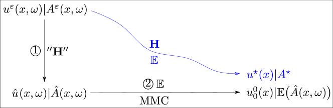
Figure 1: A schematic diagram for the two-stage stochastic homogenization method. In the first stage, the composite material with coefficient matrix $A(\frac{x}{\varepsilon},\omega)$ is equivalent to a piecewise homogeneous random material with coefficient matrix $\hat{A}(x,\omega)$. In the second stage, the homogenized solution $u_{0}^{0}(x)$ is obtained by using the MMC method. As a comparison, the classical stochastic homogenization method aims to get the stochastic homogenized solution $u^{\star}(x)$ in one step.

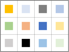
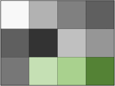
(a)  (b) (c)

Figure 2: (a) Composite material with random coefficients $A(\frac{x}{\varepsilon},\omega)$ for given $\omega$. (b) Equivalent material with random coefficients $\hat{A}(x,\omega)$ for given $\omega$, which is a constant matrix in each cell. (c) Stochastic homogenization material with deterministic coefficient $\mathbb{E}(\hat{A}(x,\omega))$.

In the second stage, we intend to solve the random diffusion problem with the equivalent (piecewise constant) coefficient matrix $\hat{A}(x,\omega)$, namely,

(13a) $$-\textnormal{div}(\hat{A}(x,\omega)\nabla\hat{u}(x,\omega)) =f(x) \qquad\textnormal{in }D,$$

(13b) $$\hat{u}(x,\omega) =0 \qquad\textnormal{on }\partial D.$$

In other words, the original oscillatory random coefficient matrix $A(\frac{x}{\varepsilon},\omega)$ is approximated by the equivalent matrix $\hat{A}(x,\omega)$ which is a constant matrix $\hat{A}^{\mathbf{k}}(\omega)$ in each block ${D}\cap\varepsilon{\cal Q}_{M}^{\mathbf{k}}$. For a given $\omega$, the computational cost for solving the homogenized problem (13) is less than that for solving the original problem (1). However, the equivalent matrix $\hat{A}(x,\omega)$ fluctuates on different blocks ${D}\cap\varepsilon{\cal Q}_{M}^{\mathbf{k}}$ due to the non-periodicity. The fluctuation leads to expensive computational costs for solving the homogenized problem (13) with small parameter $\varepsilon$ and $M={\cal O}(1)$, because the computational mesh size must be proportional to $M\varepsilon$. To overcome the difficulty, we adapt the MMC finite element method of [11] to solve (13) in an efficient way. This is possible thanks to our discovery which shows that the equivalent matrix $\hat{A}(x,\omega)$ has a nice structure, that is, it can be rewritten as a small random perturbation of the deterministic matrix $\mathbb{E}(\hat{A}(x,\cdot))$, see Section 3.2. This then sets an ideal stage for us to solve problem (13) by using the MMC method. The leading term in the MMC approximation will be defined as $u^{0}_{0}(x)$, which is the after-sought approximate solution alluded earlier, see Section 3.3.

It is important to point out that the MMC method presented in [11] can not be directly applied to a random diffusion problem (1) because its diffusion coefficient does not satisfy the weak media assumption of the MMC method (see Appendix A).

3.2 Characterization of the equivalent coefficient matrix $\hat{A}(x,\omega)$

In this subsection, we show that the equivalent matrix $\hat{A}(x,\omega)$ can be rewritten as a (small) random perturbation of a deterministic matrix. The precise statement is given in the following theorem.

Theorem 3.1.

Suppose $A(\frac{x}{\varepsilon},\omega)$ satisfies stationary hypothesis (3). Then the equivalent matrix $\hat{A}(x,\omega)$ can be rewritten as:

(14) $${\hat{A}}(x,\omega)=\mathbb{E}({\hat{A}}^{0}(\omega))+\delta A_{1}(x,\omega),$$

where ${\hat{A}}^{0}(\omega)$ denotes the equivalent matrix in any block ${D}\cap\varepsilon{\cal Q}_{M}^{\mathbf{k}}$, $A_{1}(x,\omega)=(a^{1}_{ij}(x,\omega))$ with $a^{1}_{ij}\in L^{2}(\Omega,L^{\infty}({D}))$, and $\delta$ is a (small) parameter which depends on $\varepsilon$ and $M$.

Proof 3.2.

By the stationary assumption (3), the $(i,j)$-entry of $\hat{A}(x,\omega)$ can be written as

(15) $$\hat{a}_{ij}^{\mathbf{k}}(\omega)=\frac{1}{|{\cal Q}_{M}|}\int_{{\cal Q}_{M}}(e_{i}+\nabla\mathbb{N}_{e_{i}}^{\mathbf{k}}(y,\omega))^{T}A(y+M\mathbf{k},\omega)(e_{j}+\nabla\mathbb{N}_{e_{j}}^{\mathbf{k}}(y,\omega))\textnormal{\,}dy,$$

$$\hskip 18.06749pt=\frac{1}{|{\cal Q}_{M}|}\int_{{\cal Q}_{M}}(e_{i}+\nabla\mathbb{N}_{e_{i}}^{\mathbf{k}}(y,\tau_{M\mathbf{k}}\omega))^{T}A(y,\tau_{M\mathbf{k}}\omega)(e_{j}+\nabla\mathbb{N}_{e_{j}}^{\mathbf{k}}(y,\tau_{M\mathbf{k}}\omega))\textnormal{\,}dy,$$

where the cell function $\mathbb{N}_{e_{i}}^{\mathbf{k}}(y,\tau_{M\mathbf{k}}\omega)$ satisfies

(16a) $$-\textnormal{div}[A(y,\tau_{M\mathbf{k}}\omega)(e_{i}+\nabla\mathbb{N}_{e_{i}}^{\mathbf{k}}(y,\tau_{M\mathbf{k}}\omega))]=0 \qquad\textnormal{~{}in}~{}{\cal Q}_{M},$$

(16b) $$\mathbb{N}_{e_{i}}^{\mathbf{k}}(y,\tau_{M\mathbf{k}}\omega)~{}\hbox{is}~{}{\cal Q}_{M}\hbox{-periodic}.$$

Thus, $\hat{A}^{\mathbf{k}}(\omega)=\hat{A}^{0}(\tau_{M\mathbf{k}}\omega)$, which shows that the equivalent matrix coincides with $A^{\star}_{M}(\omega)$ on each block and at each sample. Since the ergodic mapping $\tau_{k}$ preserves the measure $\mathbb{P}$, then we have

(17) $$\mathbb{E}(\hat{A}^{\mathbf{k}}(\omega))=\int\limits_{\Omega}\hat{A}^{\mathbf{k}}(\omega)\hbox{d}\mathbb{P}(\omega)=\int\limits_{\Omega}\hat{A}^{0}(\tau_{M\mathbf{k}}\omega)\hbox{d}\mathbb{P}(\tau_{M\mathbf{k}}\omega)=\mathbb{E}(\hat{A}^{0}(\omega)),$$

and

(18) $$\mathbb{V}\hbox{ar}(\hat{A}^{\mathbf{k}}(\omega)) =\int\limits_{\Omega}\left(\hat{A}^{\mathbf{k}}(\omega)-\mathbb{E}\left(\hat{A}^{\mathbf{k}}(\omega)\right)\right)^{2}\hbox{d}\mathbb{P}(\omega),$$

$$=\int\limits_{\Omega}\left(\hat{A}^{0}(\tau_{M\mathbf{k}}\omega)-\mathbb{E}\left(\hat{A}^{0}(\tau_{M\mathbf{k}}\omega)\right)\right)^{2}\hbox{d}\mathbb{P}(\tau_{M\mathbf{k}}\omega)=\mathbb{V}\hbox{ar}(\hat{A}^{\mathbf{0}}(\omega)).$$

Next, we derive a (small) random perturbation form for the equivalent matrix $\hat{A}(x,\omega)$. For a given $\mathbf{k}$, $\hat{A}^{\mathbf{k}}(\omega)=(\hat{a}_{ij}^{\mathbf{k}}(\omega))\in L^{2}(\varepsilon{\cal Q}_{M}^{\mathbf{k}})$ and the autocorrelation function of $\hat{a}_{ij}^{\mathbf{k}}(\omega)$, which is a constant, is defined by

(19) $${\hbox{Cov}_{\mathbf{k}}}=\mathbb{V}\hbox{ar}(\hat{A}^{\mathbf{k}}(\omega))=\mathbb{V}\hbox{ar}(\hat{A}^{\mathbf{0}}(\omega)).$$

Introduce the self-adjoint covariant operator ${\cal T}_{\mathbf{k}}:L^{2}(\varepsilon{\cal Q}_{M}^{\mathbf{k}})\rightarrow L^{2}(\varepsilon{\cal Q}_{M}^{\mathbf{k}})$ as

(20) $${\cal T}_{\mathbf{k}}v(\cdot):=\int_{\varepsilon{\cal Q}_{M}^{\mathbf{k}}}{\hbox{Cov}_{\mathbf{k}}}v(x)dx={\hbox{Cov}_{\mathbf{k}}}\int_{\varepsilon{\cal Q}_{M}^{\mathbf{k}}}v(x)dx\quad\forall v\in L^{2}(\varepsilon{\cal Q}_{M}^{\mathbf{k}}).$$

Let $\{(\lambda_{l},\varphi_{l})\}_{l\geq 1}$ denote a complete eigen-set of the operator ${\cal T}_{\mathbf{k}}$ with $\lambda_{1}>\lambda_{2}=\cdots=0$ and

$$\int_{\varepsilon{\cal Q}_{M}^{\mathbf{k}}}\varphi_{l}(x)\varphi_{m}(x)\hbox{d}x=\delta_{lm}\qquad l,\,m=1,\,2,\,\cdots.$$

By the Karhunen-Loéve expansion, we obtain

(21) $$\hat{a}_{ij}^{\mathbf{k}}(\omega)=\mathbb{E}(\hat{a}_{ij}^{\mathbf{k}}(\omega))+{\sum\limits_{l=1}^{\infty}}\sqrt{\lambda_{l}}\mathbf{Z}^{\mathbf{k}}_{l}(\omega)\varphi_{l}(x)=\mathbb{E}(\hat{a}_{ij}^{\mathbf{k}}(\omega))+\sqrt{\lambda_{1}}\mathbf{Z}^{\mathbf{k}}_{1}(\omega)\varphi_{1}(x),$$

where $\varphi_{1}(x)=\left|{\varepsilon{\cal Q}_{M}^{\mathbf{k}}}\right|^{-\frac{1}{2}}$ and $\mathbf{Z}^{\mathbf{k}}_{1}(\omega)$ is a standard normal variable given by

(22) $$\mathbf{Z}^{\mathbf{k}}_{1}(\omega)=\frac{\hat{a}_{ij}^{\mathbf{k}}(\omega)-\mathbb{E}(\hat{a}_{ij}^{\mathbf{k}}(\omega))}{\sqrt{\lambda_{1}}}\int_{\varepsilon{\cal Q}_{\mathbf{1}}}\varphi_{1}(x)\hbox{d}x=\sqrt{\left|{\varepsilon{\cal Q}_{\mathbf{k}}}\right|}\frac{\hat{a}_{ij}^{\mathbf{k}}(\omega)-\mathbb{E}(\hat{a}_{ij}^{\mathbf{k}}(\omega))}{\sqrt{\lambda_{1}}}.$$

The principal eigenvalue $\lambda_{1}$ satisfies

(23) $$\lambda_{1} =\frac{\int_{\varepsilon{\cal Q}_{M}^{\mathbf{k}}}{\cal T}_{\mathbf{k}}\varphi_{1}\cdot\varphi_{1}(x)\hbox{d}x}{\int_{\varepsilon{\cal Q}_{M}^{\mathbf{k}}}\varphi_{1}(x)\varphi_{1}(x)\hbox{d}x}={\hbox{Cov}_{\mathbf{k}}}\left(\int_{\varepsilon{\cal Q}_{M}^{\mathbf{k}}}\varphi_{1}(x)\hbox{d}x\right)^{2}=\left|{\varepsilon{\cal Q}_{M}^{\mathbf{k}}}\right|{\hbox{Cov}_{\mathbf{k}}},$$

which implies that

(24) $$\hat{a}_{ij}^{\mathbf{k}}(\omega)=\mathbb{E}(\hat{a}_{ij}^{\mathbf{k}}(\omega))+\sqrt{{\hbox{Cov}_{\mathbf{k}}}}\mathbf{Z}^{\mathbf{k}}_{1}(\omega)=\mathbb{E}(\hat{a}_{ij}^{\mathbf{0}}(\omega))+\sqrt{\mathbb{V}\hbox{ar}(\hat{a}_{ij}^{\mathbf{0}}(\omega))}\mathbf{Z}^{\mathbf{k}}_{1}(\omega).$$

Thus, $(i,j)$-component of $\hat{A}(x,\omega)$ satisfies

(25) $$\hat{a}_{ij}(x,\omega)=\mathbb{E}(\hat{a}_{ij}^{\mathbf{0}}(\omega))+\sqrt{\mathbb{V}\hbox{ar}(\hat{a}_{ij}^{\mathbf{0}}(\omega))}\sum\limits_{\mathbf{k}}\mathbf{Z}^{\mathbf{k}}_{1}(\omega)\Xi_{\mathbf{k}}(x).$$

where $\Xi_{\mathbf{k}}(x)$ stands for the characteristic function of the domain ${D}\cap\varepsilon{\cal Q}_{\mathbf{k}}$.

Finally, setting $\delta:=\max_{1\leq i,j\leq d}\sqrt{\mathbb{V}\hbox{ar}(\hat{a}_{ij}^{\mathbf{0}}(\omega))}$, then the equivalent matrix $\hat{A}(x,\omega)$ can be rewritten as a (small) random perturbation as stated in (14).

Remark 3.3.

The smallness of $\delta$ and the precise relationship between $\delta$ and $M$ as well as $\varepsilon$ will be given in Theorem 4.3 later in the next section.

3.3 An efficient multi-modes Monte Carlo method for solving the homogenized problem (13)

By Theorem 3.1 we know that the equivalent matrix $\hat{A}(x,\omega)$ can be rewritten as a (small) random perturbation of $\mathbb{E}({\hat{A}}^{0}(\omega))$ as given in (14). This then sets the stage for us to solve homogenized problem (13) by using the MMC method. To proceed, we first notice that $A_{1}(x,\omega)=(a^{1}_{ij}(x,\omega))$ with $a^{1}_{ij}\in L^{2}(\Omega,L^{\infty}({D}))$ satisfying

$$\mathbb{P}\bigl{\{}\omega\in\Omega;\left\|a_{ij}^{1}(\omega)\right\|_{L^{\infty}({D})}\leq\bar{a}\bigr{\}}=1.$$

In [11], the perturbation term is assumed to be in $L^{2}(\Omega,W^{1,\infty}({D}))$. However, the perturbation term $A_{1}(x,\omega)$ in (14) is not in $L^{2}(\Omega,W^{1,\infty}({D}))$ because $A_{1}(x,\omega)$ is a piecewise constant function which is discontinuous in ${D}$. Nevertheless, we show below that the MMC method can be easily extended to the case.

Due to the linear nature of the equivalent problem Eq. 13 and the small random perturbation structure of the equivalent matrix $\hat{A}(x,\omega)$, we can postulate the following multi-modes expansion for $\hat{u}(x,\omega)$:

(26) $$\hat{u}(x,\omega)={\sum_{n=0}^{\infty}\delta^{n}u^{0}_{n}(x,\omega)}.$$

Substituting Eq. 14 and Eq. 26 into Eq. 13 and matching the coefficients of $\delta^{n}$ order terms for $n=1,2,\cdots,$ we get

(27a) $$-\nabla\cdot\left(\mathbb{E}[{\hat{A}}^{0}(\omega)]\nabla u^{0}_{0}(x,\omega)\right) =f(x),$$

(27b) $$-\nabla\cdot\left(\mathbb{E}[{\hat{A}}^{0}(\omega)]\nabla u^{0}_{n}(x,\omega)\right) =\nabla\cdot\left({A}_{1}(x,\omega)\nabla u^{0}_{n-1}(x,\omega)\right)\quad\forall n\geq 1,$$

(27c) $$u^{0}_{n}(x,\omega) =0\quad\hbox{on}\quad\partial{D}\quad\forall n\geq 0.$$

Clearly, the first mode function $u_{0}^{0}(\omega,x)$ satisfies a diffusion equation with a deterministic coefficient matrix $\mathbb{E}({\hat{A}}^{0}(\omega))$ and a deterministic source term $f$. Thus, $u_{0}^{0}(\omega,x)$ is independent of $\omega$ and we relabel it as $u_{0}^{0}(x):=u_{0}^{0}(\omega,x)$. Moreover, the mode functions $\{u^{0}_{n}\}_{n\geq 0}$ satisfy a family of diffusion equations that have the same deterministic diffusion operator $L_{0}(\cdot):=-\nabla\cdot\left(\mathbb{E}[{\hat{A}}^{0}(\omega)]\nabla\cdot\right)$ but different right-hand side source terms. Furthermore, $\{u^{0}_{n}\}_{n\geq 1}$ are defined recursively with the current mode function $u_{n}$ being only dependent directly on the proceeding mode function $u_{n-1}$. The well-posedness of multi-mode functions $\{u^{0}_{n}\}$ and the corresponding error estimates will be discussed in the next section (see Theorem 4.6 and Theorem 4.8).

In this paper, we shall use the first term of the multi-modes expansion, that is, $u_{0}^{0}(x)$ as an approximation for $\hat{u}(x,\omega)$. How to efficiently compute the mode functions $\{u_{n}^{0}\}_{n\geq 1}$ is important and challenging, since $A_{1}(x,\omega)$ in the right-hand side of (27b) fluctuates in probability space and oscillates in different blocks ${D}\cap\varepsilon{\cal Q}^{\mathbf{k}}_{M}$. A natural but expensive approach is to solve (27b) for each sample $\omega$ by using a fine mesh with mesh size proportional to $M\varepsilon$, which is easily implemented but low efficient. According to Theorem 4.8 in the next section, taking $u_{0}^{0}(x)$ as an approximation of $\hat{u}(x,\omega)$ only enjoys the first order convergence rate. The convergence rate can be further improved by using more mode functions $\{u_{n}^{0}\}_{n\geq 1}$. Thus, developing more efficient numerical methods and algorithms for computing the mode functions $\{u_{n}^{0}\}_{n\geq 1}$ are important and will be addressed in future work.

4 Convergence analysis

In this section, we analyze the convergence and error estimates for the proposed two-stage stochastic homogenization method. We first show the convergence of the equivalent matrix $\hat{A}(x,\omega)$ to the homogenization matrix $A^{\star}$ as $M\to\infty$ in the next theorem.

Theorem 4.1.

Suppose $A(\frac{x}{\varepsilon},\omega)$ satisfies the stationary hypothesis (3). Let $\hat{A}(x,\omega)=(\hat{a}_{ij}(x,\omega))$ be the equivalent matrix defined by (11) and $A^{\star}=(a_{ij}^{\star})$ be defined by (6), then there holds

(28) $$\lim_{M\rightarrow\infty}\|\hat{a}_{ij}(\cdot,\omega)-a^{\star}_{ij}\|_{L^{\infty}(D)}=0\quad\text{a.s.}.$$

Proof 4.2.

By Theorem 1 in [7], we have

(29) $$\lim_{M\rightarrow\infty}\|\hat{a}^{0}_{ij}(\cdot,\omega)-a^{\star}_{ij}\|_{L^{\infty}(D)}=0\quad\hbox{a.s.}.$$

For any $\mathbf{k}$, it follows that

(30) $$\lim_{M\rightarrow\infty}\hat{a}^{\mathbf{k}}_{ij}(\omega)=\lim_{M\rightarrow\infty}\hat{a}^{0}_{ij}(\tau_{M\mathbf{k}}\omega)=a_{ij}^{\star}\quad{\color[rgb]{0,0,0}\hbox{a.s.}}\mbox{ in }L^{\infty}(D).$$

The proof is complete.

To derive the rate of convergence of $\hat{A}(x,\omega)$, we introduce the uniform mixing condition as in [7]. For a given random field $B(x,\omega)$ in $\mathbb{R}^{d}$, let ${\cal F}_{\tilde{{D}}}$ denote the $\sigma$-algebra $\sigma\{B(x),\ x\in{\tilde{{D}}}\}$. The uniform mixing coefficient of $B$ is defined as

(31) $$\gamma(s)=\sup\limits_{{\tilde{D}}_{1},{\tilde{D}}_{2}\subset\mathbb{R}^{d},\ \hbox{dist}({\tilde{D}}_{1},{\tilde{D}}_{2})\geq s}\quad\sup\limits_{\tilde{{\cal D}}_{1}\in{\cal F}_{\tilde{{\cal D}}_{1}},\tilde{{\cal D}}_{2}\in{\cal F}_{\tilde{{\cal D}}_{2}}}\left|\mathbb{P}(\tilde{{\cal D}}_{1}\cap\tilde{{\cal D}}_{2})-\mathbb{P}(\tilde{{\cal D}}_{1})\mathbb{P}(\tilde{{\cal D}}_{2})\right|.$$

In the rest of this section, we assume $\gamma(s)$ satisfies the following growth condition:

(32) $$\gamma(s)\leq c(1+s)^{-\theta}\quad\hbox{for~{}some}~{}\theta>0~{}\hbox{and}~{}\forall s>0.$$

Then we have

Theorem 4.3.

Suppose $A(\frac{x}{\varepsilon},\omega)$ satisfies the stationary hypothesis (3). Assume that the uniform mixing coefficient of $A(\frac{x}{\varepsilon},\omega)$ satisfies (32). Let $\hat{A}(x,\omega)=(\hat{a}_{ij}(x,\omega))$ and $A^{\star}=(a_{ij}^{\star})$, then there holds

(33) $$\mathbb{E}\left[(\hat{a}_{ij}(x,\cdot)-a_{ij}^{\star})^{2}\right]\leq CM^{-\zeta}\qquad\mbox{for a.e. }x\in D,$$

and there exists $\zeta=\zeta(\theta,\alpha,d)>0$ such that

(34a) $$\mathbb{V}\textnormal{ar}(\hat{a}_{ij}^{0}(\omega)) \leq CM^{-\zeta},$$

(34b) $$\delta \leq CM^{-\zeta/2}.$$

Proof 4.4.

By Theorem 5 of [7], we have

(35) $$\mathbb{E}\left[(\hat{a}^{0}_{ij}(\cdot)-a_{ij}^{\star})^{2}\right]\leq CM^{-\zeta}\qquad\mbox{for a.e. }x\in D.$$

For any $\mathbf{k}$, similar to (18), we have

(36) $$\mathbb{E}\left[(\hat{a}^{\mathbf{k}}_{ij}(\cdot)-a_{ij}^{\star})^{2}\right]=\mathbb{E}\left[(\hat{a}^{0}_{ij}(\cdot)-a_{ij}^{\star})^{2}\right]\leq CM^{-\zeta}\qquad\mbox{for a.e. }x\in D,$$

which completes the proof of (33). To show (34), using the Hölder’s inequality and (33), we get

(37) $$\bigl{(}\mathbb{E}[\hat{a}^{0}_{ij}]-a_{ij}^{\star}\bigr{)}^{2}=\left(\mathbb{E}[\hat{a}^{0}_{ij}-a_{ij}^{\star}]\right)^{2}\leq\mathbb{E}[(\hat{a}^{0}_{ij}-a_{ij}^{\star})^{2}]\leq CM^{-\zeta},$$

which implies

(38) $$\mathbb{V}\textnormal{ar}(\hat{a}_{ij}^{0}) =\mathbb{E}\left[(\hat{a}^{0}_{ij}-\mathbb{E}[\hat{a}^{0}_{ij}])^{2}\right],$$

$$\leq 2\mathbb{E}\left[(\hat{a}^{0}_{ij}-a_{ij}^{\star})^{2}\right]+2\mathbb{E}\left[(a_{ij}^{\star}-\mathbb{E}[\hat{a}^{0}_{ij}])^{2}\right],$$

$$\leq CM^{-\zeta}.$$

Thus, the proof is complete.

Remark 4.5.

One immediate corollary of Theorem 4.3 is that $\delta\rightarrow 0$ as $\varepsilon\rightarrow 0$ after taking $M=\varepsilon^{-\sigma}$ with $\sigma\in(0,1)$. This verifies that $\delta$ is indeed a small parameter.

Following Theorem 3.1 of [11], we can show the unique existence and the stability estimate for each mode $u^{0}_{n}$ in (26).

Theorem 4.6.

Assume that $A(\frac{x}{\varepsilon},\omega)\in{\cal M}(\alpha,\beta,{D})$ and $f\in L^{2}({D})$. There exists a unique solution $u^{0}_{n}\in L^{2}(\Omega,H^{1}_{0}({D}))$ to problem (27) for each $n\geq 0$ which satisfies

(39) $$\mathbb{E}(\|u_{n}^{0}\|^{2}_{H^{1}({D})})\leq C_{0}^{n+1}\|f\|^{2}_{L^{2}({D})}.$$

for some $C_{0}>0$ independent of $n$ and $\delta$.

Proof 4.7.

Using Hashin-Shtrikman bounds [16], we have $\hat{A}(x,\omega)\in{\cal M}(\alpha,\beta,{D})$. For $n=0$, the existence of a unique weak solution $u^{0}_{0}\in H^{1}_{0}({D})$ follows immediately from the Lax-Milgram Theorem (see, e.g. [12]) and there holds

(40) $$\mathbb{E}(\|u_{0}^{0}\|^{2}_{H^{1}({D})})\leq C_{0}^{1}\|f\|^{2}_{L^{2}({D})}.$$

The proof for the cases $n\geq 1$ can be done by the induction argument. Assume that (39) holds for $n=0,1,\cdots,l-1$, then $A_{1}(x,\omega)\nabla u^{0}_{n-1}\in\left[L^{2}(\Omega,L^{2}({D}))\right]^{d}$ (which is the source term in (27)). Using Theorem 3.3 in [20], there exists a unique $u_{l}^{0}\in L^{2}(\Omega,H^{1}_{0}(D))$ which solves (27) for $n=l$ and fulfills the following estimate:

(41) $$\mathbb{E}(\|u_{l}^{0}\|^{2}_{H^{1}({D})}) \leq C(D)\mathbb{E}\left(\|A_{1}(x,\omega)\nabla u^{0}_{n-1}\|^{2}_{[L^{2}({D})]^{d}}\right),$$

$$\leq dC(D)\bar{a}^{2}\mathbb{E}\left(\|\nabla u^{0}_{n-1}\|^{2}_{[L^{2}({D})]^{d}}\right),$$

$$\leq dC(D)\bar{a}^{2}\mathbb{E}\left(\|u^{0}_{n-1}\|^{2}_{H^{1}({D})}\right),$$

$$\leq C^{l+1}_{0}\|f\|^{2}_{L^{2}({D})}.$$

The proof is complete.

The next theorem establishes an estimate for the error function $\hat{u}(x,\omega)-u^{0}_{0}(x)$, which is an analogue to Theorem 3.2 of [11].

Theorem 4.8.

Suppose that $A(\frac{x}{\varepsilon},\omega)\in{\cal M}(\alpha,\beta,{D})$ satisfies stationary hypothesis (3). Assume that $\delta<1$ and $f\in L^{2}(\Omega)$, we have

(42) $$\mathbb{E}\bigl{(}\left\|\hat{u}(x,\omega)-u_{0}^{0}(x)\right\|_{{H^{1}}({D})}^{2}\bigr{)}\leqslant C_{1}{\delta^{2}}\left\|{f}\right\|_{L^{2}({D})}^{2}.$$

for some positive constant $C_{1}$ independent of $\delta$.

Proof 4.9.

Let $r(x,\omega):=\hat{u}(x,\omega)-u^{0}_{0}(x)$. Substituting (14) into (13) and combining it with the first equation of Eq. 27, we obtain

(43a) $$-\hbox{div}(\mathbb{E}({\hat{A}}(x,\omega))\nabla r(x,\omega)) =\delta\hbox{div}(A_{1}(x,\omega)\nabla\hat{u}(x,\omega)) \qquad\hbox{in }{D},$$

(43b) $$r(x,\omega) =0 \qquad\hbox{on }\partial{D}.$$

By Theorem 3.3 of [20], we get

$$\mathbb{E}\bigl{(}\left\|r\right\|_{{H^{1}}({D})}^{2}\bigr{)} \leqslant{C}(D){\delta^{2}}\mathbb{E}\bigl{(}\left\|A_{1}(x,\omega)\nabla{\hat{u}}\right\|_{[L^{2}({D})]^{d}}^{2}\bigr{)},$$

$$\leqslant d{C}(D)\bar{a}{\delta^{2}}\mathbb{E}\bigl{(}\left\|\nabla{\hat{u}}\right\|_{[L^{2}({D})]^{d}}^{2}\bigr{)},$$

$$\leqslant C_{1}{\delta^{2}}\left\|f\right\|_{L^{2}({D})}^{2}.$$

which completes the proof.

Theorem 4.10.

Let $M=C\varepsilon^{-\sigma}$ with $\sigma\in(0,1)$ and $u^{\varepsilon}$ denote the solution of problem (1). Assume that $f\in L^{2}({D})$, $A(\frac{x}{\varepsilon},\omega)\in{\cal M}(\alpha,\beta;{D})$ satisfies the stationary hypothesis (3) and is ${\cal Q}_{M}$-periodic for $\mathbb{P}$-a.s. $\omega\in\Omega$. Then there holds

(44) $$\lim_{\varepsilon\rightarrow 0}\mathbb{E}\left(\left\|{{u^{\varepsilon}}(x,\omega)-u_{0}^{0}(x)}\right\|_{{L^{2}}({D})}^{2}\right)=0.$$

Proof 4.11.

By Theorem 4.8, we have

(45) $$\mathbb{E}\Bigl{(}\left\|{{\hat{u}}(x,\omega)-u_{0}^{0}(x)}\right\|_{{L^{2}}({D})}^{2}\Bigr{)}\leq C_{1}{\delta^{2}}\left\|{f}\right\|_{{L^{2}}({D})}^{2}.$$

Since $M=C\varepsilon^{-\sigma}$ with $\sigma\in(0,1)$, it follows from Theorem 4.3 that

(46) $$\lim_{\varepsilon\rightarrow 0}\mathbb{E}\Bigl{(}\left\|{{\hat{u}}(x,\omega)-u_{0}^{0}(x)}\right\|_{{L^{2}}({D})}^{2}\Bigr{)}=0,$$

By Theorem 6.1 of [8], there hold for given $\omega\in\Omega$

(47) $$u^{\varepsilon}(x,\omega)\rightharpoonup\hat{u}(x,\omega)\quad\hbox{weakly~{}in}~{}H^{1}_{0}({D})~{}\hbox{as}~{}\varepsilon\rightarrow 0,$$

and

(48) $$u^{\varepsilon}(x,\omega)\rightarrow\hat{u}(x,\omega)\quad\hbox{strongly~{}in}~{}L^{2}({D})~{}\hbox{as}~{}\varepsilon\rightarrow 0.$$

By the triangle inequity, we get

(49) $$\lim_{\varepsilon\rightarrow 0}\mathbb{E}\left(\left\|{{u^{\varepsilon}}(x,\omega)-u_{0}^{0}(x)}\right\|_{{L^{2}}({D})}^{2}\right) \leqslant\lim_{\varepsilon\rightarrow 0}\mathbb{E}\left(\left\|{{u^{\varepsilon}}(x,\omega)-\hat{u}(x,\omega)}\right\|_{{L^{2}}({D})}^{2}\right),$$

$$\quad+\lim_{\varepsilon\rightarrow 0}\mathbb{E}\Bigl{(}\left\|{{\hat{u}}(x,\omega)-u_{0}^{0}(x)}\right\|_{{L^{2}}({D})}^{2}\Bigr{)}=0.$$

which completes the proof.

We note that the above theorem establishes the convergence of the proposed two-stage stochastic homogenization method in the case when $A(\frac{x}{\varepsilon},\omega)$ is ${\cal Q}_{M}$-periodic, the convergence for the non-periodic case remains open and will be addressed in future work.

5 Implementation algorithm for the proposed two-stage method

In this section, we address the implementation issues for the proposed two-stage stochastic homogenization method. Let $\{\omega_{s}\}_{s=1}^{L}$ be $L$ independent and identically distributed (i.i.d.) random samples in the sample space $\Omega$. Let $\mathbb{T}^{\mathbf{k}}_{h}$ stand for a quasi-uniform partition of cell ${\cal Q}^{\mathbf{k}}_{M}$ such that $\overline{{\cal Q}_{M}^{\mathbf{k}}}=\cup_{K_{\mathbf{k}}\in\mathbb{T}^{\mathbf{k}}_{h}}\overline{K_{\mathbf{k}}}$. Here we assume that the partition $\mathbb{T}^{\mathbf{k}}_{h}$ is a body-fitted grid according to the coefficients matrix $A(y+M\mathbf{k},\omega_{s})$. Let $\mathbb{V}_{r}^{{\mathbf{k}},h}$ denote the standard finite element space of degree $r$ defined by

(50) $$\mathbb{V}_{r}^{{\mathbf{k}},h}:=\{v\in H_{per}^{1}({\cal Q}^{\mathbf{k}}_{M});v|_{K_{\mathbf{k}}}~{}\hbox{is a polynomial of degree}~{}r~{}\hbox{for each}~{}K_{\mathbf{k}}\in\mathbb{T}^{\mathbf{k}}_{h}\}.$$

Here $H_{per}^{1}({\cal Q}^{\mathbf{k}}_{M})\color[rgb]{0,0,0}=\{v\in H^{1}({\cal Q}^{\mathbf{k}}_{M});~{}\hbox{such that}~{}v~{}\hbox{is}~{}{{\cal Q}^{\mathbf{k}}_{M}}\hbox{-periodic}\}$.

The finite element cell solutions $\mathbb{N}_{e_{i}}^{\mathbf{k},h}(y,\omega_{s})$ are defined as

(51) $$\left(A(y,\omega_{s})(e_{i}+\nabla\mathbb{N}_{e_{i}}^{\mathbf{k},h}(y,\omega_{s})),\nabla v^{h}\right)_{{\cal Q}^{\mathbf{k}}_{M}}=0\qquad\forall v^{h}\in\mathbb{V}_{r}^{{\mathbf{k}},h},$$

where $(u^{h},v^{h})_{{\cal Q}^{\mathbf{k}}_{M}}$ denotes the standard $L^{2}$-inner product over ${{\cal Q}^{\mathbf{k}}_{M}}$. With a help of the finite element cell solutions $\mathbb{N}_{e_{i}}^{\mathbf{k},h}(y,\omega_{s})$, the $(i,j)$-component of the approximate equivalent matrix $\hat{A}^{h}(x,\omega_{s})$ in block ${D}\cap\varepsilon{\cal Q}_{M}^{\mathbf{k}}$ is given by

(52) $$\hat{a}_{ij}^{\mathbf{k},h}(\omega_{s})=\frac{1}{|{\cal Q}_{M}|}\int_{{\cal Q}_{M}}(e_{i}+\nabla\mathbb{N}_{e_{i}}^{\mathbf{k},h}(y,\omega_{s}))^{T}A(y+M\mathbf{k},\omega_{s})(e_{j}+\nabla\mathbb{N}_{e_{j}}^{\mathbf{k},h}(y,\omega_{s}))\textnormal{d}y.$$

We define the empirical mean and variance for each component of $\hat{A}^{\mathbf{k},h}(\omega_{s})$ in block ${D}\cap\varepsilon{\cal Q}_{M}^{\mathbf{k}}$ as

(53a) $$\mu^{\mathbf{k}}_{ij,L} :=\mu_{L}\left(\hat{a}_{ij}^{\mathbf{k},h}(\omega_{s})\right)=\frac{1}{L}\sum\limits_{s=1}^{L}\hat{a}_{ij}^{\mathbf{k},h}(\omega_{s}),$$

(53b) $$\sigma^{\mathbf{k}}_{ij,L} :=\sigma_{L}\left(\hat{a}_{ij}^{\mathbf{k},h}(\omega_{s})\right)=\frac{1}{L-1}\sum\limits_{s=1}^{L}\left(\hat{a}_{ij}^{\mathbf{k},h}(\omega_{s})-\mu^{\mathbf{k}}_{ij,L}\right)^{2}.$$

Similar to [2], by the strong law of large numbers and the fact that $\hat{a}_{ij}^{\mathbf{k},h}(\omega_{s})$ is i.i.d., we have

(54) $$\mu^{\mathbf{k}}_{ij,L}\xrightarrow{L\rightarrow+\infty}\mathbb{E}\left(\hat{a}_{ij}^{\mathbf{k},h}(\omega_{s})\right)\quad\mathbb{P}\hbox{-a.s.}.$$

It follows from the central limit theorem that

(55) $$\sqrt{L}\left(\mu^{\mathbf{k}}_{ij,L}-\mathbb{E}\left(\hat{a}_{ij}^{\mathbf{k},h}(\omega_{s})\right)\right)\xrightarrow{L\rightarrow+\infty}\sqrt{\mathbb{V}\hbox{ar}\left(\hat{a}_{ij}^{\mathbf{k},h}(\omega_{s})\right)}\,{\cal N}(0,1),$$

where the convergence holds in law and ${\cal N}(0,1)$ denotes the standard Gaussian law. For sufficiently large $L$, we use $\mu^{\mathbf{k}}_{ij,L}$ as an approximation of $\mathbb{E}\left(\hat{a}_{ij}^{\mathbf{k},h}(\omega_{s})\right)$.

In the finite element approximation of the proposed two-stage stochastic homogenization method, we use $\mu_{L}=(\mu^{0}_{ij,L})$ as an approximation of $\mathbb{E}\left[\hat{A}^{0}(\omega)\right]$. Let $\mathbb{T}_{h_{0}}$ be a quasi-uniform partition of computational domain ${D}$ with mesh size $h_{0}$ such that $\overline{{D}}=\cup_{K\in\mathbb{T}_{h_{0}}}\overline{K}$. Assume $\mathbb{V}_{r}^{h_{0}}$ be the standard finite element space of order $r$ over $\mathbb{T}_{h_{0}}$ defined by

(56) $$\mathbb{V}_{r}^{h_{0}}:=\{v\in H_{0}^{1}(D);v|_{K}~{}\hbox{is a polynomial of degree}~{}r~{}\hbox{for each}~{}K\in\mathbb{T}_{h_{0}}\}.$$

The finite element approximation of the first mode function $u^{0}_{0}$ is defined by

(57) $$\left(\mu_{L}\nabla u_{0}^{0,h_{0}}(x),\nabla v^{h_{0}}\right)_{D}=(f,v^{h_{0}})_{D}\qquad\forall v^{h_{0}}\in\mathbb{V}_{r}^{h_{0}}.$$

Its implementation algorithm is given below in Algorithm 1.

Algorithm 1 The finite element two-stage stochastic homogenization method

1:  Generate a family of i.i.d. samples $\{\omega_{s}\}_{s=1}^{L}$. For each $\omega_{s}$, construct a body-fitted and quasi-uniform partition of the cell ${\cal Q}_{M}$ according to $A(y,\omega_{s})$ for $y\in{\cal Q}_{M}$.

2:  Compute finite element cell solutions $\mathbb{N}_{e_{i}}^{\mathbf{k},h}(y,\omega_{s})$ with $\mathbf{k}=0$ by solving cell problem (51) and $(i,j)$-entry of the equivalent matrix $\hat{A}^{0,h}(\omega_{s})$ by (52).

3:  Calculate the $(i,j)$-component of the empirical mean matrix $\mu_{L}$ by using (53).

4:  Solve the finite element equation Eq. 57 and obtain the finite element approximation of the first mode function $u^{0}_{0}$, which is taken as the finite element two-stage stochastic homogenization solution for the random diffusion equation (1).

Since direct simulations of the random diffusion equation (1) are computationally expensive, we use the empirical mean $\mathbb{E}(\hat{u}(x,\omega))$ of the equivalent solution for (13) as a reference solution to verify the efficiency and accuracy of the finite element two-stage stochastic homogenization method. To the end, let $\mathbb{T}_{h_{1}}$ be a quasi-uniform partition of computational domain ${D}$ with mesh size $h_{1}$ such that $\overline{{D}}=\cup_{K\in\mathbb{T}_{h_{1}}}\overline{K}$, and $\mathbb{V}_{r}^{h_{1}}$ be the standard finite element space of order $r$ defined by

(58) $$\mathbb{V}_{r}^{h_{1}}:=\{v\in H_{0}^{1}(D);v|_{K}~{}\hbox{is a polynomial of degree}~{}r~{}\hbox{for each}~{}K\in\mathbb{T}_{h_{1}}\}.$$

Let $\hat{u}^{h_{1}}(x,\omega_{s})$ be the solution of (13) with $\omega=\omega_{s}$ defined by

(59) $$\left(\hat{A}^{\mathbf{k},h}(\omega_{s})\nabla\hat{u}^{h_{1}}(x,\omega_{s}),\nabla v^{h_{1}}\right)_{D}=(f,v^{h_{1}})_{D}\qquad\forall v^{h_{0}}\in\mathbb{V}_{r}^{h_{1}}.$$

Its implementation algorithm is given below in Algorithm 2.

Algorithm 2 Algorithm for computing the reference solution

1:  Generate a family of i.i.d. samples $\{\omega\}_{s=1}^{L}$. For each $\omega_{s}$, construct a body-fitted and quasi-uniform partition of the cell ${\cal Q}^{\mathbf{k}}_{M}$ according to $A(y,\omega_{s})$ for $y\in{\cal Q}^{\mathbf{k}}_{M}$.

2:  For $\mathbf{k}\in\mathbb{Z}$ such that $\varepsilon{\cal Q}_{M}^{\mathbf{k}}\cap{D}\neq\emptyset$, compute a set of finite element cell solutions $\mathbb{N}_{e_{i}}^{\mathbf{k},h}(y,\omega_{s})$ by solving cell problem (51) and the equivalent matrix $\hat{A}^{\mathbf{k},h}(\omega_{s})=\big{(}\hat{a}_{ij}^{\mathbf{k},h}(\omega_{s})\big{)}$ by (52).

3:  For each $\omega_{s}$, solve the finite element solution $\hat{u}^{h_{1}}(x,\omega_{s})$ from (59).

4:  Calculate the reference solution for the finite element two-stage stochastic homogenization method by

$$\hat{u}^{L,h_{1}}(x)=\frac{1}{L}{\sum_{s=1}^{L}\hat{u}^{h_{1}}(x,\omega_{s})}.$$

6 Numerical experiments

In this section, we present several 2D numerical experiments to evaluate the performance of the proposed two-stage stochastic homogenization method for the random diffusion equation Eq. 1. We mainly focus on the verification of the accuracy and efficiency of the finite element approximation of the two-stage method. Our numerical experiments are performed on a desktop workstation with 16G memory and a 3.4GHz Core i7 CPU. We set $f(x)=10$ in all the tests. The cell ${\cal Q}_{M}$ in the two-stage stochastic homogenization method is taken as $Q=(0,1)^{2}$ with $M=1$. The computational domain ${D}=(0,1)^{2}$ and $\varepsilon=1/8$.

6.1 Convergence of the equivalent matrix

In this test, we study the convergence of the numerical empirical mean $\mu_{L}$ given in (53), which is used in the two-stage stochastic homogenization method. Assume ${\cal Q}_{M}=Q=Q_{1}\cup Q_{2}$ with $Q_{1}\cap Q_{2}=\emptyset$ and $Q_{2}=(0.25,0.75)^{2}$. The random coefficients in the diffusion equation Eq. 1 are chosen as

(60) $$a_{ij}(\frac{x}{\varepsilon},\omega)=\left\{\begin{split}&3\delta_{ij}+(1+\sin(2\pi\frac{x_{1}}{\varepsilon})\sin(2\pi\frac{x_{2}}{\varepsilon})\delta_{ij})Z_{\mathbf{k}}(\omega)\quad x\in\varepsilon{(Q_{1}+\mathbf{k})},\\ &300\delta_{ij}+(50+\sin(2\pi\frac{x_{1}}{\varepsilon})\sin(2\pi\frac{x_{2}}{\varepsilon})\delta_{ij})Z_{\mathbf{k}}(\omega)\quad x\in\varepsilon{(Q_{2}+\mathbf{k})}.\end{split}\right.$$

where the i.i.d. random variables $\big{(}Z_{\mathbf{k}}(\omega)\big{)}_{\mathbf{k}\in\mathbb{Z}^{2}}$ satisfy a truncated normal distribution. The probability density function for the truncated normal distribution is given by

(61) $$f(\omega,-b,b)=\left\{\begin{split}&\frac{\phi(\omega)}{\Phi(b)-\Phi(-b)}\quad&\omega\in[-b,b],\\ &0\quad&\hbox{otherwise}.\end{split}\right.$$

where $\phi(\omega)=\frac{1}{\sqrt{2\pi}}\exp{\left(-\frac{1}{2}\omega^{2}\right)}$, $\Phi(\omega)=\frac{1}{2}(1+\hbox{erf}(\omega/\sqrt{2}))$, and $b=1.5$.

For the comparison purpose, we calculate $A^{\star}_{N}=(\hat{a}_{ij,N}^{\star}(\omega))$ defined by the “cut-off” approach in (9) and take it as the reference solution. Since $A^{\star}_{N}$ converges to $A^{\star}$ as $N\rightarrow\infty$, we compare the values of $\mu_{L}$ and $A^{\star}_{N}$ by setting $L=N^{2}$ to study the convergence behavior of $\mu_{L}$. We generate a family of random variables $Z_{\mathbf{k}}(\omega)$ with $1\leq k_{1}\leq N$ and $1\leq k_{2}\leq N$. In the two-stage stochastic homogenization method, the $L$ samples are then taken as $Z_{0}(\omega_{s})=Z_{\mathbf{k}}(\omega_{s})$ with $s=k_{2}N+k_{1}$. To neglect the numerical errors coming from the finite element discretization, we use a finer quasi-uniform mesh of $\mathbb{T}^{\mathbf{k}}_{h}$ with $h=1/60$.

The numerical results for $\mu_{L}$ and $A^{\star}_{N}$ with $L=N^{2}=4,16,\cdots,1024$ are given in Table 1. From the table we observe that the relative errors for the equivalent matrix $\mu_{L}$ by taking the stochastic homogenization matrix $A^{\star}_{N}$ as reference increase as $N$ increases and stop at a small value (about 4%). Since $A^{\star}_{N}$ converges to $A^{\star}$ as $N\rightarrow\infty$, thus one can take $\mu_{L}$ as a valid approximation of $A^{\star}$. To study statistic fluctuations of the equivalent matrix $\mu_{L}$ and the stochastic homogenization matrix $A^{\star}_{N}$, we take $N=22$ as an example and run the simulation with twenty sets of i.i.d. samples. Each set consists of 484 samples. The numerical expectation and variance are given in Table 2, which clearly show that the equivalent matrix $\mu_{L}$ is a good approximation for the stochastic homogenization matrix $A^{\star}$. The total computation time for each set of the two approaches is also reported in Table 2, which demonstrates that the proposed two-stage stochastic homogenization method is more efficient than the classical stochastic homogenization method with almost the same accuracy. As a comparison to the cell problem posed on $Q_{N}$ for $N=22$ in the “periodization” stochastic homogenization method, the proposed two-stage stochastic homogenization method only needs to deal with $N^{2}$ cell problems defined on the unit cell $Q$, which is the main reason for the computational saving and the efficiency improvement. It should be pointed out that the $N^{2}$ cell problems can be solved naturally in parallel.

Table 1: The comparison of equivalent coefficients $\mu_{11,L}^{0}$ and stochastic homogenization coefficients $\hat{a}^{\star}_{11,N}$ for cell $Q_{N}$. The “Error” in the table is defined as $|\mu_{11,L}^{0}-\hat{a}^{\star}_{11,N}|/\hat{a}^{\star}_{11,N}$. The comparisons for the other three entries of the matrix are similar but not showed here.

$L=N^{2}$	$\mu_{11,L}^{0}$	$\hat{a}^{\star}_{11,N}$	Error	$L=N^{2}$	$\mu_{11,L}^{0}$	$\hat{a}^{\star}_{11,N}$	Error
4	4.9437	4.8932	0.0103	324	5.1923	5.0009	0.0383
16	5.0970	4.8020	0.0614	400	5.2592	4.9960	0.0527
36	5.3440	5.2024	0.0272	484	5.2100	4.9941	0.0432
64	5.5265	5.1084	0.0818	576	5.3724	5.0974	0.0539
100	5.3234	5.0461	0.0550	676	5.2123	4.9562	0.0517
144	5.1703	4.8894	0.0575	784	5.2520	5.0438	0.0413
196	5.1830	4.8505	0.0685	900	5.2447	5.0212	0.0445
256	5.1892	4.8886	0.0615	1024	5.1899	4.9759	0.0430

Table 2: The comparison of the numerical expectation and variance of equivalent matrix and stochastic homogenization matrix.

	Expectation	Variance	Compute time (s)
$\mu_{11,L}^{0}$	5.2130	0.1320	125.9
$\hat{a}^{\star}_{11,N}$	4.9991	0.1334	917.5

6.2 Verification of accuracy and efficiency

In order to validate the accuracy and efficiency of the proposed two-stage stochastic homogenization method, three kinds of tests (Test A, B, C) are performed in this subsection. In Test A, the composite materials have periodic structure and random coefficients; in Test B, the materials have random structure and deterministic coefficients; in Test C, both the structure and coefficients of the materials are random.

Test A: Composite materials with periodic structure and random coefficients

In this simulation, we consider two types (Type I and Type II) of composite materials with periodic structure and random parameters. The computational domain ${D}$ is decomposed into $8\times 8$ cells and all cells have the same geometry constructed by matrix (denoted by $Q_{1}$) and inclusions (denoted by $Q_{2}$). The unit cell of Type I includes a square inclusion as shown in Figure 3-(a). Figure 3-(b) shows the unit cell of Type II which contains 70 elliptical inclusions with uniform random distribution, which is generated by the take-and-place algorithm [28]. The random coefficients for matrix and inclusion are given by Eq. 60, in which i.i.d. random variables $Z_{\mathbf{k}}(\omega)$ satisfy the uniform distribution over $[-1,1]$ or a truncated normal distribution with the probability density function defined by Eq. 61.

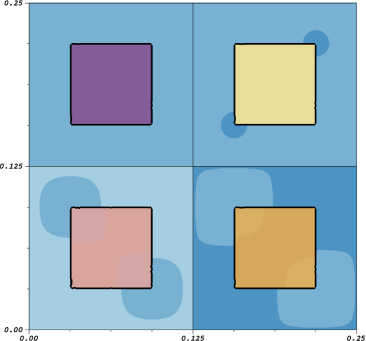
(a) (b)

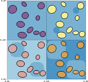
Figure 3: Test A: Composite materials with periodic structure and random coefficients. Pseudo-color of $a_{11}(x,\omega)$ on the domain $(0,\ 0.25)^{2}$ is plotted. (a) Type I: a square inclusion. (b) Type II: 10 elliptical inclusions with deterministic major/minor axis and rotation angles in each cell are taken as an example.

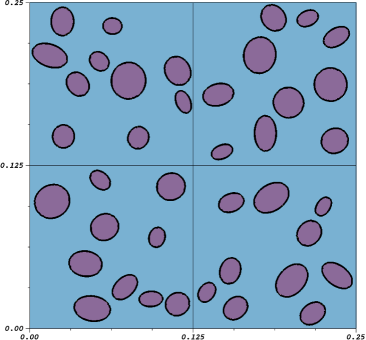
(a) (b)

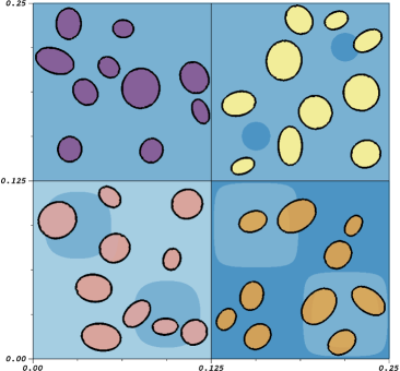
Figure 4: Pseudo-color of $a_{11}(x,\omega)$ on the domain $(0,0.25)^{2}$ is plotted. Elliptical inclusions with random position, major/minor axis, and rotation angles in each cell. (a) Test B: Composite materials with random geometry structure and deterministic coefficients. (b) Test C: Composite materials with random geometry structure and random coefficients.

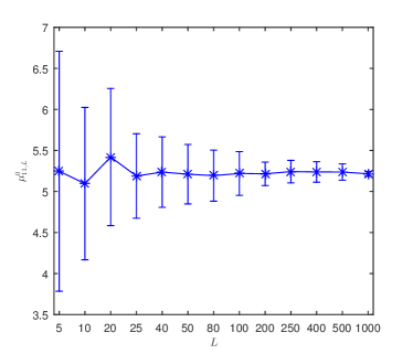
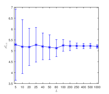
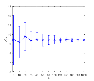
(a)  (b) (c)  (d)

Figure 5: The numerical expectation and fluctuation of equivalent coefficient $\mu^{0}_{11,L}$. (a) Type I of Test A with coefficients satisfying uniform distribution over $[-1,1]$; (b) Type I of Test A with coefficients satisfying the truncated normal distribution; (c) Type II of Test A with coefficients satisfying uniform distribution over $[-1,1]$; (d) Type II of Test A with coefficients satisfying the truncated normal distribution.

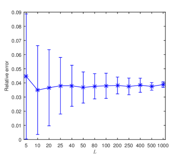
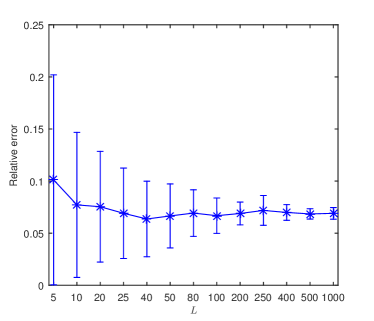
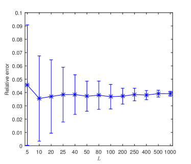
(a)  (b) (c)  (d)

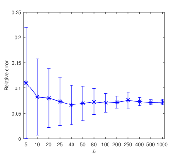
Figure 6: The relative errors of the two-stage stochastic homogenization method. (a) Type I of Test A with coefficients satisfying uniform distribution over $[-1,1]$; (b) Type I of Test A with coefficients satisfying the truncated normal distribution; (c) Type II of Test A with coefficients satisfying uniform distribution over $[-1,1]$; (d) Type II of Test A with coefficients satisfying the truncated normal distribution.

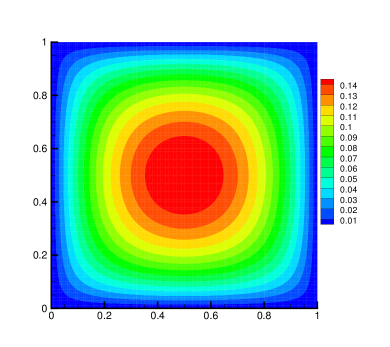
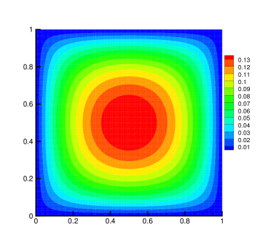
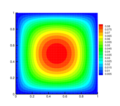
(a)  (b) (c)  (d)

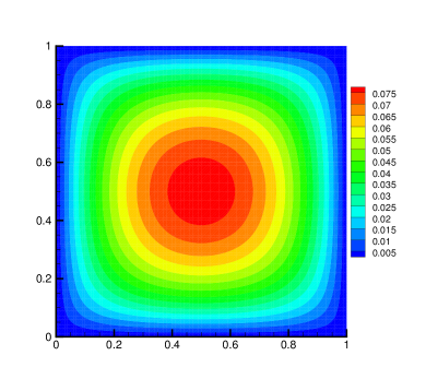
Figure 7: The contour plots of the solutions. (a) The two-stage stochastic homogenization solution $u_{0}^{0,h_{0}}$ for Type I of Test A with truncated normally distributed coefficients; (b) Reference solution $\hat{u}^{L,h_{1}}$ for Type I of Test A with standard normally distributed coefficients; (a) The two-stage stochastic homogenization solution $u_{0}^{0,h_{0}}$ for Type II of Test A with truncated normally distributed coefficients; (b) Reference solution $\hat{u}^{L,h_{1}}$ for Type II of Test A with standard normally distributed coefficients.

Test B: Composite materials with random structure and deterministic coefficients

In this test, we consider composite materials with random structure and deterministic coefficients. As shown in Figure 4-(a), the computational domain ${D}$ is decomposed into $8\times 8$ cells and each cell contains 10 elliptical inclusions with uniform random distribution sample $\omega$, which is generated by the take-and-place algorithm [28]. Denote ${D}_{1}(\omega)$ as the matrix subdomain and ${D}_{2}(\omega)$ the inclusion subdomain. The deterministic coefficients in both subdomains are taken as

$$a_{ij}(\frac{x}{\varepsilon},\omega)=\left\{\begin{split}&3\delta_{ij}&\quad x\in{D}_{1}(\omega),\\ &300\delta_{ij}&\quad x\in{D}_{2}(\omega).\end{split}\right.$$

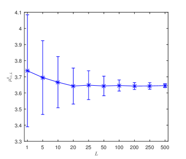
(a)  (b)

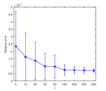
Figure 8: Test B: (a) the numerical expectation and fluctuation of equivalent coefficient $\mu^{0}_{11,L}$; (b) the relative errors of the two-stage stochastic homogenization method.

Test C: Composite materials with random structure and random coefficients

This test can be viewed as a combination of Test A and B. As shown in Figure 4-(b), the computational domain ${D}$ is decomposed into $8\times 8$ cells and each cell contains 10 elliptical inclusions with uniform random distribution sample $\omega_{1}$, which is generated by the take-and-place algorithm [28]. Let ${D}_{1}(\omega_{1})$ and ${D}_{2}(\omega_{1})$ have the same definitions as in Test B. The random coefficients in both subdomains are now defined as

$$a_{ij}(\frac{x}{\varepsilon},\omega)=\left\{\begin{split}&3\delta_{ij}+(1+\sin(2\pi\frac{x_{1}}{\varepsilon})\sin(2\pi\frac{x_{2}}{\varepsilon})\delta_{ij})Z_{\mathbf{k}}(\omega_{2})&x\in{D}_{1}(\omega_{1})\cap\varepsilon{(Q+\mathbf{k})},\\ &300\delta_{ij}+(50+\sin(2\pi\frac{x_{1}}{\varepsilon})\sin(2\pi\frac{x_{2}}{\varepsilon})\delta_{ij})Z_{\mathbf{k}}(\omega_{2})&x\in{D}_{2}(\omega_{1})\cap\varepsilon{(Q+\mathbf{k})}.\end{split}\right.$$

where the i.i.d. random variables $\big{(}Z_{\mathbf{k}}(\omega_{2})\big{)}_{\mathbf{k}\in\mathbb{Z}^{2}}$ satisfy the uniform distribution over $[-1,1]$ or the truncated normal distribution with the probability density function defined by (61) .

Table 3: The number of degrees of freedom (Dof) used in the three tests.

	Test A (Type I)	Test A (Type II), Test B,C
Cell problem	3,600	14,400
Homogenized problem	10,000	10,000

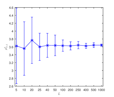
(a)  (b)

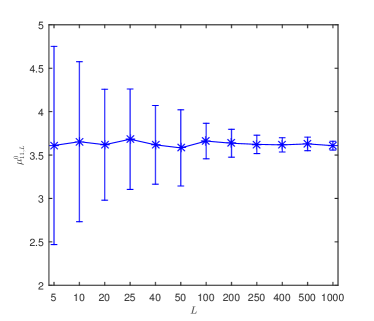
Figure 9: The numerical expectation and fluctuation of equivalent coefficient $\mu^{0}_{11,L}$. (a) Test C with uniformly distributed coefficients; (b) Test C with truncated normally distributed coefficients.

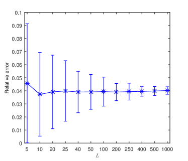
(a)  (b)

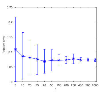
Figure 10: The relative errors of the two-stage stochastic homogenization method. (a) Test C with uniformly distributed coefficients; (b) Test C with truncated normally distributed coefficients.

Table 4: Total compute times for the three test cases by using the two-stage stochastic homogenization method (“Present”) and the reference method (“Reference”).

	Method	Total time(s)	Cell problem(s)	Homogenized problem(s)
Test A	Reference	6,415.9	2,569.9	3,846.0
	Present	2,704.4	2,703.9	0.5
Test B	Reference	10,115.5	6,258.3	3,857.2
	Present	6,337.3	6,334.4	2.9
Test C	Reference	17,294.9	13,434.1	3,860.8
	Present	12,753.5	12,750.5	3.0

In each simulation, the unit cell $Q$ is partitioned into a body-fitted and quasi-uniform mesh $\mathbb{T}^{\mathbf{k}}_{h}$. The mesh size $h=1/60$ is used for Type I of Test A and $h=1/120$ for the other tests. The equation (57) is solved on a quasi-uniform partition $\mathbb{T}_{h_{0}}$ of the domain ${D}$ with the mesh size $h_{0}=1/100$. For comparison, we calculate the reference solution by solving (59) on another quasi-uniform partition $\mathbb{T}_{h_{1}}$ of the domain ${D}$ with the mesh size $h_{1}=1/100$. The relative error for the two-stage stochastic homogenization solution is defined as $\|u_{0}^{0,h_{0}}-\hat{u}^{L,h_{1}}\|_{L^{2}({D})}/\|\hat{u}^{L,h_{1}}|_{L^{2}({D})}$. In Test A and Test C, the total number of samples is taken as $10,000$. Those samples are then divided into several subsets and they consist of respectively the following numbers of samples $L=5,\ 10,\ 20,\ \cdots,\ 1,000$. In Test B, the total number of samples is taken as $5,000$ and the numbers of samples in the subsets are set as $L=5,\ 10,\ 20,\ \cdots,\ 500$.

The numerical expectations and fluctuations of the equivalent coefficients $\mu_{11,L}^{0}$ for all three tests are presented in Figures 5, 8, and 9. The numerical results, which are not shown, for the other entries of the equivalent matrix are similar. We observe that as the number ($L$) of the total samples increases, the expectation tends to stabilize and the variance gradually decreases. Moreover, we also observe that when $L=500\sim 1,000$ the two-stage stochastic homogenization method can obtain a stable and accurate equivalent matrix. Figures 6, 8, and 10 show the relative errors of the computed two-stage stochastic homogenization solutions, and the numerical results show that the relative errors reduce to a relatively low value (about 0.1%-10%) as the number of the total samples increases. Figure 7 displays the contour plots of the computed two-stage stochastic homogenization solutions and the reference solution. The consistency of the two solutions is clearly seen. Table 3 presents the computational costs for solving the cell problem and the homogenized problem. Since the homogenized problem is only solved once in the two-stage stochastic homogenization method, the computational cost for the proposed method is much less than the other approach in which the homogenized problem must be solved $L$ times. The CPU times used by Test A, B, and C are respectively given in Table 4. Those numerical results demonstrate that the two-stage stochastic homogenization method is computationally quite efficient and accurate.

7 Conclusion

In this paper, we developed a two-stage stochastic homogenization method for solving diffusion equations with random fast oscillation coefficients. In the first stage, the proposed method constructs an equivalent matrix by solving a cell problem posed on the finite cell ${\cal Q}_{M}$. It was proved that the equivalent matrix converges to the stochastic homogenized matrix as the cell size goes to infinity. To balance the efficiency and accuracy, the proposed two-stage stochastic homogenization method usually chooses a suitable large cell and calculates the empirical mean by taking $L$ samples in the probability space. In the second stage, the approximation of the homogenized problem, which is a random diffusion problem, is solved by employing an efficient multi-modes Monte Carlo method, after having shown that the equivalent matrix can be rewritten as a small random perturbation of some deterministic matrix. As a result, the proposed two-stage method provides an efficient procedure to obtain an approximation to the homogenized solution. The efficiency and accuracy of the two-stage stochastic homogenization method were validated by several numerical experiments on some benchmark problems.

In summary, we propose a new stochastic homogenization method with a two-stage procedure, which is different with the classical stochastic homogenization method or “cut-off” procedure. This appears to be the first attempt to separate the computational difficulty caused by the spatial fast oscillation of the solution and that caused by the randomness of the solution, so they can be overcome separately using different strategies. Besides, the convergence of the solution of the spatially homogenized equation (from the first stage) to the solution of the original random diffusion equation is established and the optimal rate of convergence is also obtained for the proposed multi-modes Monte Carlo method. This appears to be the first attempt to obtain the explicit convergence order for the stochastic homogenization method.

Appendix A: The property of random matrix $A(\frac{x}{\varepsilon},\omega)$

The random matrix $A(\frac{x}{\varepsilon},\omega)$ of the composite materials usually does not satisfy the small random perturbation or can not be rewritten into the desired form by the Karhunen-Loéve expansion. The precise statement is supported by the following example. Thus, the MMC finite element method of [11] can not be applied directly to solving the random diffusion problem (1).

Example 1: Let $Q=Q_{1}\cup Q_{2}$ with $Q_{1}\cap Q_{2}=\emptyset$. Assume ${D}_{1}=\cup_{\mathbf{k}\in\mathbb{Z}^{d}}{D}\cap\varepsilon(Q_{1}+\mathbf{k})$ and ${D}_{2}=\cup_{\mathbf{k}\in\mathbb{Z}^{d}}{D}\cap\varepsilon(Q_{2}+\mathbf{k})$. The entries of the random matrix $A(\frac{x}{\varepsilon},\omega)$ are taken as

(A.1) $$a_{ij}\Bigl{(}\frac{x}{\varepsilon},\omega\Bigr{)}=\left\{\begin{gathered}a_{ij,1}(1+\omega)\quad x\in{{D}_{1}},\hfill\\ a_{ij,2}(1+\omega)\quad x\in{{D}_{2}}.\hfill\\ \end{gathered}\right.$$

where $a_{ij,1}$ and $a_{ij,2}$ are two distinct constants and $\omega$ is a uniformly distributed scalar random variable over $[0,1]$. The autocorrelation function of $a_{ij}(\frac{x}{\varepsilon},\omega)$ is given by

(A.2) $$\begin{gathered}{\hbox{Cov}_{a}}(s,t)=\mathbb{E}\left[\left(a_{ij}\Bigl{(}\frac{s}{\varepsilon},\omega\Bigr{)}-\mathbb{E}\left[a_{ij}(\frac{s}{\varepsilon},\omega)\right]\right)\left(a_{ij}\Bigl{(}\frac{t}{\varepsilon},\omega\Bigr{)}-\mathbb{E}\left[a_{ij}\Bigl{(}\frac{t}{\varepsilon},\omega\Bigr{)}\right]\right)\right],\\ \qquad\qquad=\left\{\begin{gathered}\frac{1}{12}a_{ij,1}a_{ij,2}\quad\quad\hbox{for}~{}s\in{{D}_{1}},~{}t\in{{D}_{2}},~{}\hbox{or}~{}s\in{{D}_{2}},~{}t\in{{D}_{1}},\hfill\\ \frac{1}{12}a_{ij,1}^{2}\quad\quad\hbox{for}~{}s\in{{D}_{1}},~{}t\in{{D}_{1}},\hfill\\ \frac{1}{12}a_{ij,2}^{2}\quad\quad\hbox{for}~{}s\in{{D}_{2}},~{}t\in{{D}_{2}}.\hfill\\ \end{gathered}\right.\end{gathered}$$

Therefore, ${\hbox{Cov}_{a}}(s,t)$ is a discontinuous function. By Lemma 4.2 of [1], the Karhunen-Loéve expansion does not give the required small random perturbation form for random matrix $A(\frac{x}{\varepsilon},\omega)$.

Moreover, suppose that the $(i,j)$-component of $A(\frac{x}{\varepsilon},\omega)$ can be rewritten as $a_{ij}(\frac{x}{\varepsilon},\omega)=a_{ij}^{0}(x)+\delta a^{1}_{ij}(\frac{x}{\varepsilon},\omega)$ with $a^{1}_{ij}\in L^{2}(\Omega,L^{\infty}({D}))$ satisfying

$$\mathbb{P}\bigl{\{}\omega\in\Omega;\left\|a_{ij}^{1}(\omega)\right\|_{L^{\infty}({D})}\leq\bar{a}\bigr{\}}=1,$$

where $\bar{a}$ is a constant independent of small parameter $\delta$. Thus, we have

$$a^{1}_{ij}\Bigl{(}\frac{x}{\varepsilon},\omega\Bigr{)}=\frac{a_{ij}\bigl{(}\frac{x}{\varepsilon},\omega\bigr{)}-a_{ij}^{0}(x)}{\delta},$$

Let $\omega_{1}\in\Omega_{1}=[0,\frac{1}{4}]$ and $\omega_{2}\in\Omega_{2}=[\frac{3}{4},1]$, it follows that

(A.3) $$\Bigl{\|}a^{1}_{ij}\Bigl{(}\frac{x}{\varepsilon},\omega_{1}\Bigr{)}\Bigr{\|}_{L^{\infty}({D})} +\Bigl{\|}a^{1}_{ij}\Bigl{(}\frac{x}{\varepsilon},\omega_{2}\Bigr{)}\Bigr{\|}_{L^{\infty}({D})},$$

(A.4) $$\geq\frac{\|{a_{ij}(\frac{x}{\varepsilon},\omega_{1})-a_{ij}(\frac{x}{\varepsilon},\omega_{2})\|_{L^{\infty}({D})}}}{\delta},$$

(A.5) $$\geq\frac{1}{2\delta}\max\{a_{ij,1},\,a_{ij,2}\}.$$

which contradicts with the condition $\mathbb{P}\bigl{\{}\omega\in\Omega;\left\|a_{ij}^{1}(\omega)\right\|_{L^{\infty}({D})}\leq\bar{a}\bigr{\}}=1$ with $\bar{a}$ being independent of small parameter $\delta$. Therefore, the random matrix $A(\frac{x}{\varepsilon},\omega)$ can not be rewritten as $A_{ij}(\frac{x}{\varepsilon},\omega)=A_{ij}^{0}(x)+\delta A^{1}_{ij}(\frac{x}{\varepsilon},\omega)$.

References

- [1] A. Alexanderian, A brief note on the Karhunen-Lòve expansion, arXiv:1509.07526, 2015.
- [2] A. Anantharaman, R. Costaouec, C. L. Bris, F. Legoll, and F. Thomines, Introduction to numerical stochastic homogenization and the related computational challenges: some recent developments, in Multiscale Modeling and Analysis for Materials Simulation, World Scientific Press, pp. 197–272, 2012.
- [3] A. Anantharaman and C. Le Bris, A numerical approach related to defect-type theories for some weakly random problems in homogenization, Multiscale. Model. Sim., 9 (2011), pp. 513–544.
- [4] A. Anantharaman and C. Le Bris, Elements of mathematical foundations for numerical approaches for weakly random homogenization problems, Commun. Comput. Phys., 11 (2012), pp. 1103–1143.
- [5] A. Bensoussan, J. L. Lions, and G. Papanicolaou, Asymptotic Analysis for Periodic Structures, vol. 374, American Mathematical Society, 2011.
- [6] X. Blanc, C. Le Bris, and P. L. Lions, Stochastic homogenization and random lattices, J. Math. Pure. Appl., 88 (2007), pp. 34–63.
- [7] A. Bourgeat and A. Piatnitski, Approximations of effective coefficients in stochastic homogenization, Ann. I. H. Poincare-Pr., 40 (2004), pp. 153–165.
- [8] D. Cioranescu and P. Donato, An Introduction to Homogenization, vol. 17, Oxford University Press, 1999.
- [9] J. Cui, Y. Shan, and L. Cao, Multi-scale analysis method for composite materials with random distribution and related structures, in the Proceedings of 8th Intern. Confer. Composites Engineering, 161–163, 2001.
- [10] M. Duerinckx, A. Gloria, and F. Otto, The structure of fluctuations in stochastic homogenization, Commun. Math. Phys., 377 (2020), pp. 259–306.
- [11] X. Feng, J. Lin, and C. Lorton, A multimodes Monte Carlo finite element method for elliptic partial differential equations with random coefficients, Int. J. Uncertain. Quan., 6 (2016), pp. 429–443.
- [12] D. Gilbarg and N. S. Trudinger, Elliptic Partial Differential Equations of Second Order, vol. 224, Springer, 2015.
- [13] I. Gitman, H. Askes, and L. Sluys, Representative volume: Existence and size determination, Eng. Fract. Mech., 74 (2007), pp. 2518–2534.
- [14] A. Gloria and F. Otto, An optimal error estimate in stochastic homogenization of discrete elliptic equations, Ann. Appl. Probab., 22 (2012), pp. 1–28.
- [15] I. G. Graham, F. Y. Kuo, D. Nuyens, R. Scheichl, and I. H. Sloan, Quasi-Monte Carlo methods for elliptic PDEs with random coefficients and applications, J. Comput. Phys., 230 (2011), pp. 3668–3694.
- [16] Z. Hashin and S. Shtrikman, A variational approach to the theory of the effective magnetic permeability of multiphase materials, J. Appl. Phys., 33 (1962), pp. 3125–3131.
- [17] S. M. Kozlov, Averaging of random operators, Matemat. Sbornik, 151 (1979), pp. 188–202.
- [18] Y. Li and J. Cui, The multi-scale computational method for the mechanics parameters of the materials with random distribution of multi-scale grains, Compos. Sci. Technol., 65 (2005), pp. 1447–1458.
- [19] J. Liu, J. Lu, and X. Zhou, Efficient rare event simulation for failure problems in random media, SIAM J. Sci. Comput., 37 (2015), pp. A609–A624.
- [20] O. A. Oleïnik, A. Shamaev, and G. Yosifian, Mathematical Problems in Elasticity and Homogenization, Elsevier, 2009.
- [21] G. C. Papanicolaou, Boundary value problems with rapidly oscillating random coefficients, Colloq. Math. Soc. Janos Bolyai., 27 (1979), pp. 853–873.
- [22] A. Pozhidaev and V. Yurinskiĭ, On the error of averaging symmetric elliptic systems, Izv. Akad. Nauk SSSR Ser. Mat., 53 (1989), pp. 851–867.
- [23] K. Sab, On the homogenization and the simulation of random materials, Euro. J. Mech. A-Solid., 11 (1992), pp. 585–607.
- [24] R. Suribhatla, I. Jankovic, A. Fiori, A. Zarlenga, and G. Dagan, Effective conductivity of an anisotropic heterogeneous medium of random conductivity distribution, Multiscale. Model. Sim., 9 (2011), pp. 933–954.
- [25] L. Tartar, The General Theory of Homogenization: a Personalized Introduction, vol. 7, Springer Science & Business Media, 2009.
- [26] Q. D. To and G. Bonnet, FFT based numerical homogenization method for porous conductive materials, Comput. Method. Appl. M., 368 (2020), pp. 113–160.
- [27] S. S. Vel and A. J. Goupee, Multiscale thermoelastic analysis of random heterogeneous materials: Part i: Microstructure characterization and homogenization of material properties, Comp. Mater. Sci., 48 (2010), pp. 22–38.
- [28] Z. Wang, A. Kwan, and H. Chan, Mesoscopic study of concrete I: generation of random aggregate structure and finite element mesh, Comput. Struct., 70 (1999), pp. 533–544.
- [29] X. F. Xu and X. Chen, Stochastic homogenization of random elastic multi-phase composites and size quantification of representative volume element, Mech. Mater., 41 (2009), pp. 174–186.
- [30] Y. Nie and Y. Wu, An efficient approach to determine the effective properties of random heterogeneous materials, High Temperature Ceramic Matrix Composites 8: Ceramic Transactions, pp. 23–28, 2014.
- [31] V. V. Yurinskii, Averaging of symmetric diffusion in random medium, Siberian. Math. J., 27 (1986), pp. 603–613.