Bayesian Inference via Sparse Hamiltonian Flows

Abstract

A Bayesian coreset is a small, weighted subset of data that replaces the full dataset during Bayesian inference, with the goal of reducing computational cost. Although past work has shown empirically that there often exists a coreset with low inferential error, efficiently constructing such a coreset remains a challenge. Current methods tend to be slow, require a secondary inference step after coreset construction, and do not provide bounds on the data marginal evidence. In this work, we introduce a new method—sparse Hamiltonian flows—that addresses all three of these challenges. The method involves first subsampling the data uniformly, and then optimizing a Hamiltonian flow parametrized by coreset weights and including periodic momentum quasi-refreshment steps. Theoretical results show that the method enables an exponential compression of the dataset in a representative model, and that the quasi-refreshment steps reduce the KL divergence to the target. Real and synthetic experiments demonstrate that sparse Hamiltonian flows provide accurate posterior approximations with significantly reduced runtime compared with competing dynamical-system-based inference methods.

1 Introduction

Bayesian inference provides a coherent approach to learning from data and uncertainty assessment in a wide variety of complex statistical models. Two standard methodologies for performing Bayesian inference in practice are Markov chain Monte Carlo (MCMC) [1; 2; 3, Ch. 11,12] and variational inference (VI) [4, 5]. MCMC simulates a Markov chain that targets the posterior distribution. In the increasingly common setting of large-scale data, most exact MCMC methods are intractable. This is essentially because simulating each MCMC step requires an (expensive) computation involving each data point, and many steps are required to obtain inferential results of a reasonable quality. To reduce cost, a typical approach is to perform the computation for a random subsample of the data, rather than the full dataset, at each step [6, 7, 8, 9, 10] (see [11] for a recent survey). However, recent work shows that the speed benefits are outweighed by the drawbacks; uniformly subsampling at each step causes MCMC to either mix slowly or provide poor inferential approximation quality [12, 13, 14, 11, 15]. VI, on the other hand, posits a family of approximations to the posterior and uses optimization to find the closest member, enabling the use of scalable stochastic optimization algorithms [16, 17]. While past work involved simple parametric families, recent work has developed flow families based on Markov chains [18, 19]—and in particular, those based on Langevin and Hamiltonian dynamics [20, 21, 22, 23, 24, 25]. However, because these Markov chains are typically designed to target the posterior distribution, each step again requires a computation involving all the data, making KL minimization and sampling slow. Repeated subsampling to reduce cost has the same issues that it does in MCMC.

Although repeated subsampling in each step of a Markov chain (for MCMC or VI) is not generally helpful, recent work on Bayesian coresets [26] has provided empirical evidence that there often exists a fixed small, weighted subset of the data—a coreset—that one can use to replace the full dataset in a standard MCMC or VI inference method [27]. In order for the Bayesian coreset approach to be practically useful, one must (1) find a suitable coreset that provides a good posterior approximation; and (2) do so quickly enough that the speed-up of inference is worth the time it takes to find the coreset. There is currently no option that satisfies these two desiderata. Importance weighting methods [26] are fast, but do not provide adequate approximations in practice. Sparse linear regression methods [28, 29, 30] are fast and sometimes provide high-quality approximations, but are very difficult to tune well. And sparse variational methods [27, 31] find very high quality coreset approximations without undue tuning effort, but are too slow to be practical.

This work introduces three key insights. First, we can uniformly subsample the dataset once to pick the points in the coreset (the weights still need to be optimized). This selection is not only significantly simpler than past algorithms; we show that it enables constructing an exact coreset—with KL divergence 0 to the posterior—of size $O(\log_{2}(N))$ for $N$ data points in a representative model (Proposition 3.1). Second, we can then construct a normalizing flow family based on Hamiltonian dynamics [32, 21, 22] that targets the coreset posterior (parametrized by coreset weights) rather than the expensive full posterior. This method address all of the current challenges with coresets: it enables tractable i.i.d. sampling, provides a known density and normalization constant, and is tuned using straightforward KL minimization with stochastic gradients. It also addresses the inefficiency of Markov-chain-based VI families, as the Markov chain steps are computed using the inexpensive coreset posterior density rather than the full posterior density. The final insight is that past momentum tempering methods [21] do not provide sufficient flexibility for arbitrary approximation to the posterior, even in a simple setting (Proposition 3.2). Thus, we introduce novel periodic momentum quasi-refreshment steps that provably reduce the KL objective (Propositions 3.3 and A.2). The paper concludes with real and synthetic experiments, demonstrating that sparse Hamiltonian flows compare favourably to both current coreset compression methods and variational flow-based families. Proofs of all theoretical results may be found in the appendix.

It is worth noting that Hamiltonian flow posterior approximations based on a weighted data subsample were also developed in concurrent work in the context of variational annealed importance sampling [33], and subsampling prior to weight optimization was developed in concurrent work on MCMC [34]. In this work, we focus on incorporating Bayesian coresets into Hamiltonian-based normalizing flows to obtain fast and accurate posterior approximations.

2 Background

2.1 Bayesian coresets

We are given a target probability density $\pi(\theta)$ for variables $\theta\in\mathbb{R}^{d}$ that takes the following form:

$$\pi(\theta)=\frac{1}{Z}\exp\left(\sum_{n=1}^{N}f_{n}(\theta)\right)\pi_{0}(\theta).\addcontentsline{lla}{section}{\numberline{\string\crtrefnumber{eq:target}}{e}q:target}$$ (2)

In a Bayesian inference problem with i.i.d. data, $\pi_{0}$ is the prior density, the $f_{n}$ are the log-likelihood terms for $N$ data points, and the normalization constant is in general not known. The goal is to take samples from the distribution corresponding to density $\pi(\theta)$.

In order to avoid the $\Theta(N)$ cost of evaluating $\log\pi(\theta)$ or $\nabla\log\pi(\theta)$ (at least one of which must be conducted numerous times in most standard inference algorithms), Bayesian coresets [26] involve replacing the target with a surrogate density of the form

$$\pi_{w}(\theta)=\frac{1}{Z(w)}\exp\left(\sum_{n=1}^{N}w_{n}f_{n}(\theta)\right)\pi_{0}(\theta),\addcontentsline{lla}{section}{\numberline{\string\crtrefnumber{eq:coreset}}{e}q:coreset}$$ (3)

where $w\in\mathbb{R}^{N}$, $w\geq 0$ are a set of weights. If $w$ has at most $M\ll N$ nonzeros, the $O(M)$ cost of evaluating $\log\pi_{w}(\theta)$ or $\nabla\log\pi_{w}(\theta)$ is a significant improvement upon the original $\Theta(N)$ cost.

The baseline method to construct a coreset is to draw a uniformly random subsample of $M$ data points, and give each a weight of $N/M$; although this method is fast in practice, it typically generates poor posterior approximations. More advanced techniques generally involve significant user tuning effort [26, 28, 29, 30]. The current state-of-the-art black box approach formulates the problem as variational inference [27, 31] and provides a stochastic gradient scheme using samples from $\pi_{w}$,

$$w^{\star}=\operatornamewithlimits{arg\,min}_{w\in\mathbb{R}_{+}^{N}}\mathrm{D_{KL}}\mathchoice{\left({{{{\pi_{w}||\pi}}}}\right)}{({{{{\pi_{w}||\pi}}}})}{({{{{\pi_{w}||\pi}}}})}{({{{{\pi_{w}||\pi}}}})}\quad\text{s.t.}\quad\|w\|_{0}\leq M.$$ (4)

Empirically, this method tends to produce very high-quality coresets [27]. However, to estimate the gradient at each iteration of the optimization, we require MCMC samples from the weighted coreset posterior at that iteration. While generating MCMC samples from a sparse coreset posterior is not expensive, it is difficult to tune the algorithm to ensure the quality of these MCMC samples across iterations (as the weights, and thus the coreset posterior, change each iteration). The amount of tuning effort required makes the application of this method too slow to be practical. Once the coreset is constructed, all of the aforementioned methods require a secondary inference algorithm to take draws from $\pi_{w}$. Further, since $Z(w)$ is not known in general, it is not tractable to use these methods to bound the marginal evidence $Z$.

2.2 Hamiltonian dynamics

In this section we provide a very brief overview of some important aspects of a special case of Hamiltonian dynamics and its use in statistics; see [35] for a more comprehensive overview. The differential equation below in Eq. 5 describes how a (deterministic) Hamiltonian system with position $\theta_{t}\in\mathbb{R}^{d}$, momentum $\rho_{t}\in\mathbb{R}^{d}$, differentiable negative potential energy $\log\pi(\theta_{t})$, and kinetic energy $\frac{1}{2}\rho_{t}^{T}\rho_{t}$ evolves over time $t\in\mathbb{R}$:

$$\frac{\mathrm{d}\rho_{t}}{\mathrm{d}t} =\nabla\log\pi(\theta_{t})\qquad\frac{\mathrm{d}\theta_{t}}{\mathrm{d}t}=\rho_{t}.\addcontentsline{lla}{section}{\numberline{\string\crtrefnumber{eq:ham_dynamics}}{e}q:ham_{d}ynamics}$$ (5)

For $t\in\mathbb{R}$, define the mappings $H_{t}:\mathbb{R}^{2d}\to\mathbb{R}^{2d}$ that take $(\theta_{s},\rho_{s})\mapsto(\theta_{s+t},\rho_{s+t})$ under the dynamics in Eq. 5. These mappings have two key properties that make Hamiltonian dynamics useful in statistics. First, they are invertible, and preserve volume in the sense that $\left|\det\nabla H_{t}\right|=1$. In other words, they provide tractable density transformations: for any density $q$ on $\mathbb{R}^{2d}$ and pushforward $q_{t}$ on $\mathbb{R}^{2d}$ under the mapping $H_{t}$, we have that $q_{t}(\cdot,\cdot)=q\left(H_{t}^{-1}(\cdot,\cdot)\right)$. Second, the augmented target density $\bar{\pi}(\theta,\rho)$ on $\mathbb{R}^{2d}$ corresponding to independent draws from $\pi$ and $\mathcal{N}(0,I)$,

$$\bar{\pi}(\theta,\rho)\propto\pi(\theta)\cdot\exp\left(-\frac{1}{2}\rho^{T}\rho\right),\addcontentsline{lla}{section}{\numberline{\string\crtrefnumber{eq:bpi}}{e}q:bpi}$$ (6)

is invariant under the mappings $H_{t}$, i.e., $\bar{\pi}(H_{t}(\cdot,\cdot))=\bar{\pi}(\cdot,\cdot)$. Given these properties, Hamiltonian Monte Carlo [35, 36] constructs a Gibbs sampler for $\bar{\pi}$ that interleaves Hamiltonian dynamics with periodic stochastic momentum refreshments $\rho\sim\mathcal{N}(0,I)$. Upon completion, the $\rho$ component of the samples can be dropped to obtain samples from the desired target $\pi$.

In practice, one approximately simulates the dynamics in Eq. 5 using the leapfrog method, which involves interleaving three discrete transformations with step size $\epsilon>0$,

$$\hat{\rho}_{k+1} =\rho_{k}+\frac{\epsilon}{2}\nabla\log\pi(\theta_{k}) \theta_{k+1} =\theta_{k}+\epsilon\hat{\rho}_{k+1} \rho_{k+1} =\hat{\rho}_{k+1}+\frac{\epsilon}{2}\nabla\log\pi(\theta_{k+1}).\addcontentsline{lla}{section}{\numberline{\string\crtrefnumber{eq:leapfrog}}{e}q:leapfrog}$$ (7)

Denote the map constructed by applying these three steps in sequence $T_{\epsilon}:\mathbb{R}^{2d}\to\mathbb{R}^{2d}$. As the transformations in Eq. 7 are all shear, $T_{\epsilon}$ is also volume-preserving, and for small enough step size $\epsilon$ it nearly maintains the target invariance. Note also that evaluating a single application of $T_{\epsilon}$ is of $O(Nd)$ complexity, which is generally expensive in the large-data (large-$N$) regime.

2.3 VI via Hamiltonian dynamics

Since the mapping $T_{\epsilon}$ is invertible and volume-preserving, it is possible to tractably compute the density of the pushforward of a reference distribution $q(\cdot,\cdot)$ under repeated applications of it. In addition, this repated application of $T_{\epsilon}$ resembles the steps of Hamiltonian Monte Carlo (HMC) [35], which we know converges in distribution to the target posterior distribution. [21, 22] use these facts to construct a normalizing flow [32] VI family. However, there are two issues with this methodology. First, the $O(Nd)$ complexity of evaluating each step $T_{\epsilon}$ makes training and simulating from this flow computationally expensive. Second, Hamiltonian dynamics on its own creates a flow with insufficient flexibility to match a target $\bar{\pi}$ of interest. In particular, given a density $q(\cdot,\cdot)$ and pushforward $q_{t}(\cdot,\cdot)$ under $H_{t}$, we have

$$\forall t\in\mathbb{R},\quad\mathrm{D_{KL}}\mathchoice{\left({{{{q_{t}||\bar{\pi}}}}}\right)}{({{{{q_{t}||\bar{\pi}}}}})}{({{{{q_{t}||\bar{\pi}}}}})}{({{{{q_{t}||\bar{\pi}}}}})}=\mathrm{D_{KL}}\mathchoice{\left({{{{q||\bar{\pi}}}}}\right)}{({{{{q||\bar{\pi}}}}})}{({{{{q||\bar{\pi}}}}})}{({{{{q||\bar{\pi}}}}})}.\addcontentsline{lla}{section}{\numberline{\string\crtrefnumber{eq:constantkl}}{e}q:constantkl}$$ (8)

In other words, Hamiltonian dynamics itself cannot reduce the KL divergence to $\bar{\pi}$; it simply interchanges potential and kinetic energy. [21] address this issue by instead deriving their flow from tempered Hamiltonian dynamics: for an integrable tempering function $\gamma:\mathbb{R}\to\mathbb{R}$,

$$\frac{\mathrm{d}\rho_{t}}{\mathrm{d}t} =\nabla\log\pi(\theta_{t})-\gamma(t)\rho_{t}\qquad\frac{\mathrm{d}\theta_{t}}{\mathrm{d}t}=\rho_{t}.\addcontentsline{lla}{section}{\numberline{\string\crtrefnumber{eq:tempered_ham_dynamics}}{e}q:tempered_{h}am_{d}ynamics}$$ (9)

The discretized version of the dynamics in Eq. 9 corresponds to multiplying the momentum by a tempering value $\alpha_{k}>0$ after the $k^{\text{th}}$ application of $T_{\epsilon}$. By scaling the momentum, one provides the normalizing flow with the flexibility to change the kinetic energy at each step. However, we show later in Proposition 3.2 that just tempering the momentum does not provide the required flow flexibility, even for a simple representative Gaussian target.

A related line of work uses the mapping $T_{\epsilon}$ for variational annealed importance sampling [23, 24, 25]. The major difference between these methods and the normalizing flow-based methods is that the auxiliary variable is (partially) stochastically refreshed via $\rho\sim\mathcal{N}(0,I)$ after applications of $T_{\epsilon}$. One is then forced to minimize the KL divergence between the joint distribution of $\theta$ and all of the auxiliary momentum variables under the variational and augmented target distributions.

3 Sparse Hamiltonian flows

In this section we present sparse Hamiltonian flows, a new method to construct and draw samples from Bayesian coreset posterior approximations. We first present a method and supporting theory for selecting the data points to be included in the coreset, then discuss building a sparse flow with these points, and finally introduce quasi-refreshment steps to give the flow family enough flexibility to match the target distribution. Sparse Hamiltonian flows enables tractable i.i.d. sampling, provides a tractable density and normalization constant, and is constructed by minimizing the KL divergence to the posterior with simple stochastic gradient estimates.

3.1 Selection via subsampling

The first step in our algorithm is to choose a uniformly random subsample of $M$ points from the full dataset; these will be the data points that comprise the coreset. Without loss of generality, we assume these are the first $M$ points. The key insight in this work is that while subsampling with importance weighting does not typically provide good coreset approximations [26], a uniformly random subset of the $N$ log-likelihood potential functions $\{f_{1},\dots,f_{M}\}$ still provides a good basis for approximation with high probability. Proposition 3.1 provides the precise statement of this result for a representative example model Eq. 10. In particular, Proposition 3.1 asserts that as long as we set our coreset size $M$ to be proportional to $d\log_{2}N$, the optimal coreset posterior approximation will be exact, i.e., have 0 KL divergence to the true posterior, with probability at least $1-N^{-\frac{d}{2}}(\log_{2}N)^{\frac{d}{2}}$. Thus we achieve an exponential compression of the dataset, $N\to\log_{2}N$, without losing any fidelity. Note that we will still need a method to choose the weights $w_{1},\dots,w_{M}$ for the $M$ points, but the use of uniform selection rather than a one-at-a-time approach [29, 28, 27] substantially simplifies the construction. In Proposition 3.1, $C$ is the universal constant from [37, Corollary 1.2], which provides an upper bound on the number of spherical balls of some fixed radius needed to cover a $d$-dimensional unit sphere.

Proposition 3.1.

Consider a Bayesian Gaussian location model:

$$\theta \sim\mathcal{N}(0,I)\quad\text{and}\quad\forall n\in[N],\quad X_{n}\overset{\textrm{\tiny{i.i.d.}\@}}{\sim}\mathcal{N}(\theta,I),\addcontentsline{lla}{section}{\numberline{\string\crtrefnumber{eq:simple_model}}{e}q:simple_{m}odel}$$ (10)

where $\theta,X_{n}\in\mathbb{R}^{d}$ for $d\in\mathbb{N}$. Suppose the true data generating parameter $\theta=0$, and set $M=\log_{2}(A_{d}N^{d}(\log N)^{-d/2})+C$ where $A_{d}=e^{\frac{d}{2}}d^{\frac{3}{2}}\log(1+d)$. Then the optimal coreset $\pi_{w^{\star}}$ for the model Eq. 10 built using a uniform subsample of data of size $M$ satisfies

$$\limsup_{N\to\infty}\frac{\mathbb{P}\left(\mathrm{D_{KL}}\mathchoice{\left({{{{\pi_{w^{\star}}||\pi}}}}\right)}{({{{{\pi_{w^{\star}}||\pi}}}})}{({{{{\pi_{w^{\star}}||\pi}}}})}{({{{{\pi_{w^{\star}}||\pi}}}})}\neq 0\right)}{N^{-\frac{d}{2}}(\log N)^{\frac{d}{2}}}\leq 1.$$ (11)

3.2 Sparse flows

Upon taking a uniform subsample of $M$ data points from the full dataset, we consider the sparsified Hamiltonian dynamics initialized at $\theta_{0},\rho_{0}\sim q(\cdot,\cdot)$ for reference density $q(\cdot,\cdot)$,

$$\frac{\mathrm{d}\rho_{t}}{\mathrm{d}t} =\nabla\log\pi_{w}(\theta_{t})\qquad\frac{\mathrm{d}\theta_{t}}{\mathrm{d}t}=\rho_{t}.\addcontentsline{lla}{section}{\numberline{\string\crtrefnumber{eq:wham_dynamics}}{e}q:wham_{d}ynamics}$$ (12)

Much like the original Hamiltonian dynamics for the full target density, the sparsified Hamiltonian dynamics Eq. 12 targets the augmented coreset posterior with density $\bar{\pi}_{w}(\theta,\rho)$ on $\mathbb{R}^{2d}$,

$$\bar{\pi}_{w}(\theta,\rho)\propto\pi_{w}(\theta)\exp\left(-\frac{1}{2}\rho^{T}\rho\right).$$ (13)

Discretizing these dynamics yields a leapfrog method similar to Eq. 7 with three interleaved steps,

$$\hat{\rho}_{k+1} =\rho_{k}+\frac{\epsilon}{2}\nabla\log\pi_{w}(\theta_{k}) \theta_{k+1} =\theta_{k}+\epsilon\hat{\rho}_{k+1} \rho_{k+1} =\hat{\rho}_{k+1}+\frac{\epsilon}{2}\nabla\log\pi_{w}(\theta_{k+1}).\addcontentsline{lla}{section}{\numberline{\string\crtrefnumber{eq:wleapfrog}}{e}q:wleapfrog}$$ (14)

Denote the map constructed by applying these three steps in sequence $T_{w,\epsilon}:\mathbb{R}^{2d}\to\mathbb{R}^{2d}$. Like the original leapfrog method, these transformations are both invertible and shear, and thus preserve volume; and for small enough step size $\epsilon$, they approximately maintain the invariance of $\bar{\pi}_{w}(\theta,\rho)$. However, since $w$ only has the first $M$ entries nonzero,

$$\nabla\log\pi_{w}(\theta_{k}) =\sum_{m=1}^{M}w_{m}\nabla\log f_{m}(\theta_{k}),$$ (15)

and thus a coreset leapfrog step can be taken in $O(Md)$ time, as opposed to $O(Nd)$ time in the original approach. Given that Proposition 3.1 recommends setting $M\approx d\log_{2}(N)$, we have achieved an exponential reduction in computational cost of running the flow.

However, as before, the weighted sparse leapfrog flow is not sufficient on its own to provide a flexible variational family. In particular, we know that $T_{w,\epsilon}$ nearly maintains the distribution $\bar{\pi}_{w}$ as invariant. We therefore need a way to modify the distribution of the momentum variable $\rho$. One option is to include a tempering of the form Eq. 9 into the sparse flow. However, Proposition 3.2 shows that even optimal tempering does not provide the flexibility to match a simple Gaussian target $\bar{\pi}$.

Proposition 3.2.

Let $\theta_{t},\rho_{t}\in\mathbb{R}$ follow the tempered Hamiltonian dynamics Eq. 9 targeting $\pi=\mathcal{N}(0,\sigma^{2})$, $\sigma>0$, with initial distribution $\theta_{0}\sim\mathcal{N}(\mu,1)$, $\rho_{0}\sim\mathcal{N}(0,\beta^{2})$ for initial center $\mu\in\mathbb{R}$ and momentum scale $\beta>0$. Let $q_{t}$ be the distribution of $(\theta_{t},\rho_{t})$. Then

$$\inf_{t>0,\beta>0,\gamma:\mathbb{R}_{+}\to\mathbb{R}}\mathrm{D_{KL}}\mathchoice{\left({{{{q_{t}||\bar{\pi}}}}}\right)}{({{{{q_{t}||\bar{\pi}}}}})}{({{{{q_{t}||\bar{\pi}}}}})}{({{{{q_{t}||\bar{\pi}}}}})} \geq\log\frac{1+\mu^{2}}{4\sigma}.$$ (16)

Note that if $\gamma(t)=0$ identically, then $\forall t\geq 0$, $\mathrm{D_{KL}}\mathchoice{\left({{{{q_{t}||\bar{\pi}}}}}\right)}{({{{{q_{t}||\bar{\pi}}}}})}{({{{{q_{t}||\bar{\pi}}}}})}{({{{{q_{t}||\bar{\pi}}}}})}=\mathrm{D_{KL}}\mathchoice{\left({{{{q_{0}||\bar{\pi}}}}}\right)}{({{{{q_{0}||\bar{\pi}}}}})}{({{{{q_{0}||\bar{\pi}}}}})}{({{{{q_{0}||\bar{\pi}}}}})}$.

The intuition behind Proposition 3.2 is that while adding a tempering $\gamma(t)$ enables one to change the total energy by scaling the momentum, it does not allow one fine enough control on the distribution of the momentum. For example, if $\mathbb{E}[\rho]\neq 0$ under the current flow approximation, we cannot scale the momentum to force $\mathbb{E}[\rho]=0$ as it should be under the augmented target; intuitively, we also need the ability to shift or recenter the momentum as well.

Algorithm 1 SparseHamFlow

$\theta_{0}$, $\rho_{0}$, $w$, $\epsilon$, $\lambda$, $L$, $R$

$J\leftarrow 0$, and $(\theta,\rho)\leftarrow(\theta_{0},\rho_{0})$

for $r=1,\dots,R$ do

     for $\ell=1,\dots,L$ do

         Sparse flow leapfrog:

         $\theta,\rho\leftarrow T_{w,\epsilon}(\theta,\rho)$

     end for

     Accumulate log Jacobian determinant:

     $J\leftarrow J+\log\mathchoice{\left|{{{{\det\frac{\partial R_{\lambda_{r}}}{\partial\rho}(\rho,\theta)}}}}\right|}{|{{{{\det\frac{\partial R_{\lambda_{r}}}{\partial\rho}(\rho,\theta)}}}}|}{|{{{{\det\frac{\partial R_{\lambda_{r}}}{\partial\rho}(\rho,\theta)}}}}|}{|{{{{\det\frac{\partial R_{\lambda_{r}}}{\partial\rho}(\rho,\theta)}}}}|}$

     Quasi-refreshment:

     $\rho\leftarrow R_{\lambda_{r}}(\rho,\theta)$

end for

return $\theta,\rho,J$

Algorithm 2 Estimate_ELBO

$q$, $\pi_{0}$, $w$, $\epsilon$, $\lambda$, $L$, $R$, $S$

$(\theta_{0},\rho_{0})\sim q(\cdot,\cdot)$

Forward pass:

$\theta,\rho,J\leftarrow$ SparseHamFlow$\left(\theta_{0},\rho_{0},w,\epsilon,\lambda,L,R\right)$

Obtain unbiased ELBO estimate:

$(n_{1},\dots,n_{S})\overset{\textrm{\tiny{i.i.d.}\@}}{\sim}{\sf{Unif}}(\{1,2,\dots,N\})$

$\log\bar{p}\leftarrow\log\pi_{0}(\theta)+\frac{N}{S}\sum_{s=1}^{S}f_{n_{s}}(\theta)+$

$\quad\quad\quad\quad\log\mathcal{N}(\rho\mid 0,I)$

$\log\bar{q}\leftarrow q(\theta_{0},\rho_{0})-J$

return $\log\bar{p}-\log\bar{q}$

3.3 Quasi-refreshment

Rather than resampling the momentum variable from its target marginal—which removes the ability to evaluate the density of $\theta_{t},\rho_{t}$—in this work we introduce deterministic quasi-refreshment moves that enable the flow to strategically update the momentum without losing the ability to compute the density and normalization constant of $\theta_{t},\rho_{t}$ (i.e., we construct a normalizing flow [32]). Here we introduce the notion of marginal quasi-refreshment, which tries to make the marginal distribution of $\rho_{t}$ match the corresponding marginal distribution of the augmented target $\bar{\pi}_{w}$. Proposition 3.3 shows that marginal quasi-refreshment is guaranteed to reduce the KL divergence.

Proposition 3.3.

Consider the state $\theta_{t},\rho_{t}\in\mathbb{R}^{d}$ of the flow at step $t$, and the augmented target distribution $\theta,\rho\sim\bar{\pi}$. Suppose that we have a bijection $R:\mathbb{R}^{d}\to\mathbb{R}^{d}$ such that $R(\rho_{t})\overset{d}{=}\rho$. Then

$$\mathrm{D_{KL}}\mathchoice{\left({{{{\theta_{t},R(\rho_{t})||\theta,\rho}}}}\right)}{({{{{\theta_{t},R(\rho_{t})||\theta,\rho}}}})}{({{{{\theta_{t},R(\rho_{t})||\theta,\rho}}}})}{({{{{\theta_{t},R(\rho_{t})||\theta,\rho}}}})} =\mathrm{D_{KL}}\mathchoice{\left({{{{\theta_{t},\rho_{t}||\theta,\rho}}}}\right)}{({{{{\theta_{t},\rho_{t}||\theta,\rho}}}})}{({{{{\theta_{t},\rho_{t}||\theta,\rho}}}})}{({{{{\theta_{t},\rho_{t}||\theta,\rho}}}})}-\mathrm{D_{KL}}\mathchoice{\left({{{{\rho_{t}||\rho}}}}\right)}{({{{{\rho_{t}||\rho}}}})}{({{{{\rho_{t}||\rho}}}})}{({{{{\rho_{t}||\rho}}}})}.$$ (17)

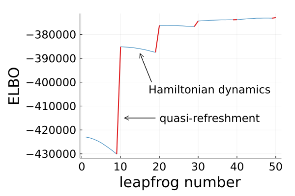
Figure 1: ELBO across leapfrog steps.

See Appendix A for the proof of Proposition 3.3 and a general treatment of quasi-refreshment; for simplicity, we focus on the type of quasi-refreshment that we use in the experiments. In particular, if we are willing to make an assumption about the marginal distribution of $\rho_{t}$ at step $t$ of the flow, we can introduce a tunable family of functions $R_{\lambda}$ with parameters $\lambda$ that is flexible enough to set $R_{\lambda}(\rho_{t})\overset{d}{=}\rho$ for some $\lambda$, and include optimization of $\lambda$ along with the coreset weights. It is important to note that this assumption on the distribution of $\rho_{t}$ is not related to the posterior $\pi$. As an example, in this work we assume that $\rho_{t}\sim\mathcal{N}(\mu,\Lambda^{-1})$ for some unknown mean $\mu$ and diagonal precision $\Lambda$, which enables us to simply set

$$R_{\lambda}(x)=\Lambda\left(x-\mu\right).\addcontentsline{lla}{section}{\numberline{\string\crtrefnumber{eq:marginal_standardization}}{e}q:marginal_{s}tandardization}$$ (18)

We then include $\lambda=(\mu,\Lambda)$ as parameters to be optimized along with the coreset weights $w$ (each quasi-refreshment step will have its own set of parameters $\mu,\Lambda$). Even when this assumption does not hold exactly, the resulting form of Eq. 18 enables the refreshment step to both shift and scale (i.e., standardize) the momentum as desired, and is natural to implement as part of a single optimization routine.

Fig. 1 provides an example of the effect of quasi-refreshment in a synthetic Gaussian location model (see Section 4.1 for details). In particular, it shows the evidence lower bound (ELBO) as a function of leapfrog step number in a trained sparse Hamiltonian flow with the quasi-refreshment scheme in Eq. 18. While the estimated ELBO values stay relatively stable across leapfrog steps in between quasi-refreshments (as expected by Eq. 8), the quasi-refreshment steps (colored red) cause the ELBO to increase drastically. We note that the ELBO does not stay exactly constant because the Hamiltonian dynamics targets the coreset posterior instead of the true posterior, and is simulated approximately using leapfrog steps. As the series of transformations brings the approximated density closer to the target, the quasi-refreshment steps no longer change the ELBO much, signalling the convergence of the flow’s approximation of the target. It is thus clear that the marginal quasi-refreshments indeed decrease the KL, as shown in Proposition 3.3.

3.4 Algorithm

In this section, we describe the procedure for training and generating samples from a sparse Hamiltonian flow. As a normalizing flow, a sparse Hamiltonian flow can be trained by maximizing the augmented ELBO using usual stochastic gradient methods (e.g. as in [32]), where the transformations follow Eq. 14 with a periodic quasi-refreshment. Here and in the experiments we focus on the shift-and-scale quasi-refreshment in Eq. 18.

We begin by selecting a subset of $M$ data points chosen uniformly randomly from the full data. Next we select a total number $R$ of quasi-refreshment steps, and a number $L$ of leapfrog steps between each quasi-refreshment. The flow parameters to be optimized consist of the quasi-refreshment parameters $\lambda=(\lambda_{r})_{r=1}^{R}$, the $M$ coreset weights $w=(w_{m})_{m=1}^{M}$, and the leapfrog step sizes $\epsilon=(\epsilon_{i})_{i=1}^{d}$; note that we use a separate step size $\epsilon_{i}$ per latent variable dimension $i$ in Eq. 14 [35, Sec. 4.2]. This modification enables the flow to fit nonisotropic target distributions.

We initialize the weights to $N/M$ (i.e., a uniform coreset), and select an initial step size for all dimensions. We use a warm start to initialize the parameters $\lambda_{r}=(\mu_{r},\Lambda_{r})$ of the quasi-refreshments. Specifically, using the initial leapfrog step sizes and coreset weights, we pass a batch of samples from the reference density $q(\cdot,\cdot)$ through the flow up to the first quasi-refreshment step. We initialize $\mu_{1},\Lambda_{1}$ to the empirical mean and diagonal precision of the samples at that point. We then apply the initialized first quasi-refreshment to the momentum, proceed with the second sequence of leapfrog steps, and repeat until we have initialized all quasi-refreshments $r=1,\dots,R$.

Once the parameters are initialized, we log-transform the step sizes, weights, and quasi-refreshment diagonal scaling matrices to make them unconstrained during optimization. We obtain an unbiased estimate of the augmented ELBO gradient by applying automatic differentiation [38, 39] to the ELBO estimation function Algorithm 2, and optimize all parameters jointly using a gradient-based stochastic optimization technique such as SGD [40, 41] and ADAM [42]. Once trained, we can obtain samples from the flow via Algorithm 1.

4 Experiments

In this section, we compare our method against other Hamiltonian-based VI methods and Bayesian coreset construction methods. Specifically, we compare the quality of posterior approximation, as well as the training and sampling times of sparse Hamiltonian flows (SHF), Hamiltonian importance sampling (HIS) [21], and unadjusted Hamiltonian annealing (UHA) [23] using real and synthetic datasets. We compare with two variants of HIS and UHA: “-Full,” in which we train using in-flow minibatching as suggested by [21, 23], but compute evaluation metrics using the full-data flow; and “-Coreset,” in which we base the flow on a uniformly subsampled coreset. We also include sampling times of adaptive HMC and NUTS [43, Alg. 5 and 6] using the full dataset. Finally, we compare the quality of coresets constructed by SHF to those obtained using uniform subsampling (UNI) and Hilbert coresets with orthogonal matching pursuit (Hilbert-OMP) [28, 44]. All experiments are performed on a machine with an Intel Core i7-12700H processor and 32GB memory. Code is available at https://github.com/NaitongChen/Sparse-Hamiltonian-Flows. Details of the experiments are in Appendix B.

4.1 Synthetic Gaussian

We first demonstrate the performance of SHF on a synthetic Gaussian-location model,

$$\theta \sim\mathcal{N}(0,I)\quad\text{and}\quad\forall n\in[N],\quad X_{n}\overset{\textrm{\tiny{i.i.d.}\@}}{\sim}\mathcal{N}(\theta,cI),$$ (19)

where $\theta,X_{n}\in\mathbb{R}^{d}$. We set $c=100$, $d=10$, $N=10,000$. This model has a closed from posterior distribution $\pi=\mathcal{N}\left(\frac{\sum_{n=1}^{N}X_{n}}{c+N},\frac{c}{c+N}I\right)$. More details may be found in Section B.1.

Fig. 2(a) compares the ELBO values of SHF, HIS, and UHA across all optimization iterations. We can see that SHF and UHA-Full result in the highest ELBO, and hence tightest bound on the log normalization constant of the target. In this problem, since we have access to the exact posterior distribution in closed form, we can also estimate the $\theta$-marginal KL divergence directly, as shown in Fig. 2(b). Here we see the posterior approximation produced by SHF provides a significantly lower KL than the other competing methods. Figs. 2(c), 2(d), 2(e) and 2(f) show, through a number of other metrics, that SHF provides a higher quality posterior approximation than others. It is worth noting that while the relative covariance error for SHF takes long to converge, we observe a monotonic downward trend in both the relative mean error and KL divergence of SHF. This means that for this particular problem, our method finds the centre of the target before fine tuning the covariance. We also note that a number of metrics go up for UHA-full because it operates on the augmented space based on a sequence of distributions that bridge some simple initial distribution and the target distribution. Therefore, it is not guaranteed that all steps of optimization improve the quality of approximation on the marginal space of the latent variables of interest, which is what the plots in Fig. 2 show.

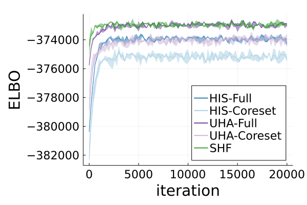
(a) (a)

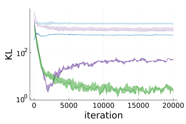
(b) (b)

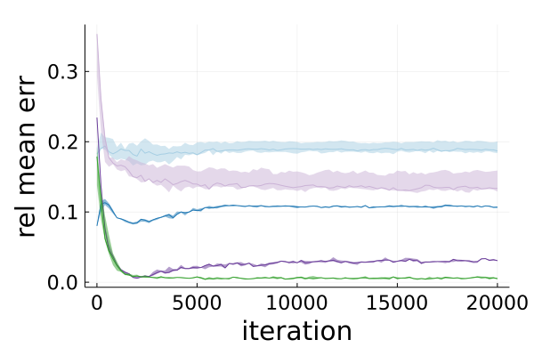
(c) (c)

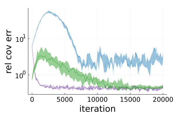
(d) (d)

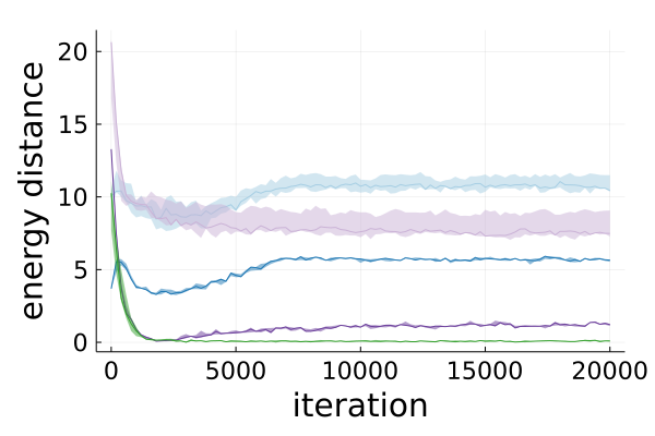
(e) (e)

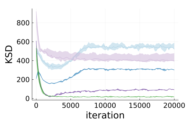
(f) (f)

Figure 2: ELBO (Fig. 2(a)), KL divergence (Fig. 2(b)), relative 2-norm mean error (Fig. 2(c)), relative Frobenius norm covariance error (Fig. 2(d)), energy distance (Fig. 2(e)), and IMQ KSD [45] (Fig. 2(f)) for synthetic Gaussian. The lines indicate the median, and error regions indicate 25${}^{\text{th}}$ to 75${}^{\text{th}}$ percentile from 5 runs.

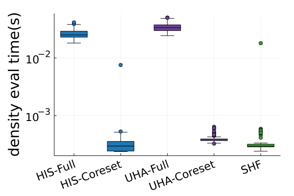
(a) (a)

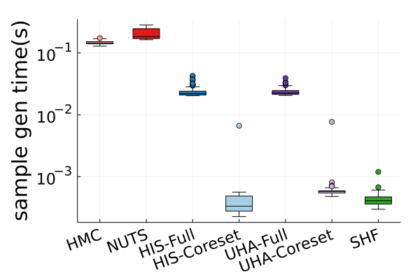
(b) (b)

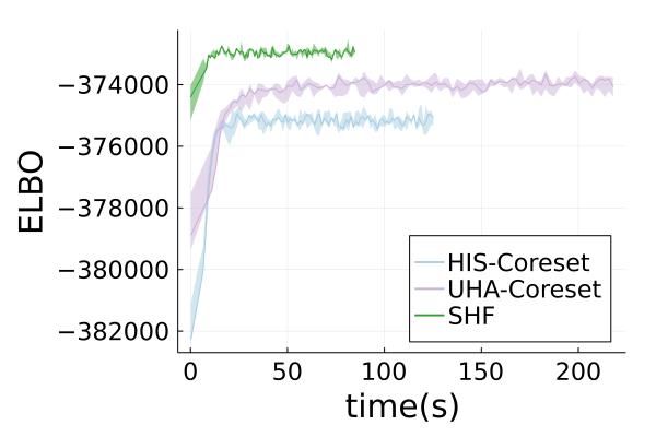
(c) (c)

Figure 3: Density evaluation (Fig. 3(a)) and sample generation time (Fig. 3(b)) (100 samples), and ELBO versus time during training (Fig. 3(c)) for synthetic Gaussian. The lines indicate the median, and error regions indicate 25${}^{\text{th}}$ to 75${}^{\text{th}}$ percentile from 5 runs.

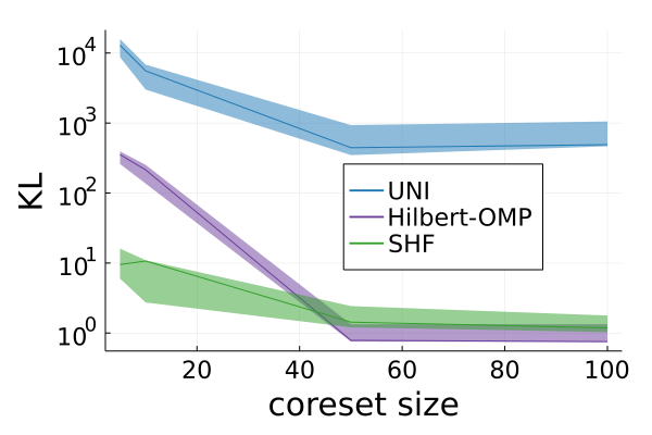
(a) (a)

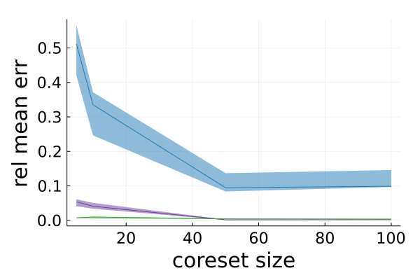
(b) (b)

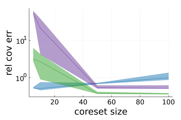
(c) (c)

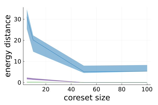
(d) (d)

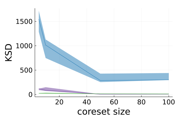
(e) (e)

Figure 4: Estimated KL divergence (Fig. 4(a)), relative 2-norm mean error (Fig. 4(b)), relative Frobenius norm covariance error (Fig. 4(c)), energy distance (Fig. 4(d)), and IMQ KSD (Fig. 4(e)) versus coreset size. The lines indicate the median, and error regions indicate 25${}^{\text{th}}$ to 75${}^{\text{th}}$ percentile from 5 runs.

Figs. 3(a) and 3(b) show the time required for each method to evaluate the density of the joint distribution of $\theta,\rho$ and to generate samples. It is clear that the use of a coreset improves the density evaluation and sample generation time by more than an order of magnitude. Fig. 3(c) compares the training times of SHF, HIS-Coreset, and UHA-Coreset (recall that due to the use of subsampled minibatch flow dynamics, HIS-Full and UHA-Full share the same training time as their -Coreset versions). The relative training speeds generally match those of sample generation from the target posterior.

Finally, Fig. 4 compares the quality of coresets constructed via SHF, uniform subsampling (UNI), and Hilbert coresets with orthogonal matching pursuit (Hilbert-OMP). Note that in this problem, the Laplace approximation is exact (the true posterior is Gaussian), and hence Hilbert-OMP constructs a coreset using samples from the true posterior. Despite this, SHF provides coresets of comparable quality, in addition to enabling tractable i.i.d. sampling, density evaluation, normalization constant bounds, and straightforward construction via stochastic optimization.

4.2 Bayesian linear regression

In the setting of Bayesian linear regression, we are given a set of data points $(x_{n},y_{n})^{N}_{n=1}$, each consisting of features $x_{n}\in\mathbb{R}^{p}$ and response $y_{n}\in\mathbb{R}$, and a model of the form

$$\begin{bmatrix}\beta&\log\sigma^{2}\end{bmatrix}^{T}\sim\mathcal{N}(0,I),\quad\forall n\in[N],\quad y_{n}\mid x_{n},\beta,\sigma^{2}\overset{\textrm{\tiny{indep}}}{\sim}\mathcal{N}\left(\begin{bmatrix}1&x_{n}^{T}\end{bmatrix}\beta,\sigma^{2}\right),\addcontentsline{lla}{section}{\numberline{\string\crtrefnumber{eq:linreg_model}}{e}q:linreg_{m}odel}$$ (20)

where $\beta\in\mathbb{R}^{p+1}$ is a vector of regression coefficients and $\sigma^{2}\in\mathbb{R}_{+}$ is the noise variance. The dataset that we use consists of $N=100,000$ flights, each containing $p=10$ features (e.g., distance of the flight, weather conditions, departure time, etc), and the response variable is the difference, in minutes, between the scheduled and actual departure times. More details can be found in Section B.2.

Since we no longer have the posterior distribution in closed form, we estimate the mean and covariance using $5000$ samples from Stan [46] and treat them as the true posterior mean and covariance. Figs. 5(a), 5(b) and 5(c) show the marginal KL, relative mean error, and relative covariance error of SHF, HIS, and UHA, where the marginal KL is estimated using the Gaussian approximation of the posterior with the estimated mean and covariance. Here we also include the posterior approximation obtained using the Laplace approximation as a baseline. We see that SHF provides the highest quality posterior approximation. Furthermore, Fig. 5(d) shows that SHF provides a significant improvement in the marginal KL compared with competing coreset constructions UNI and Hilbert-OMP. This is due to the true posterior no longer being Gaussian; the Laplace approximation required by Hilbert-OMP fails to capture the shape of the posterior. Additional plots comparing the quality of posterior approximations using various other metrics can be found in Section B.2.

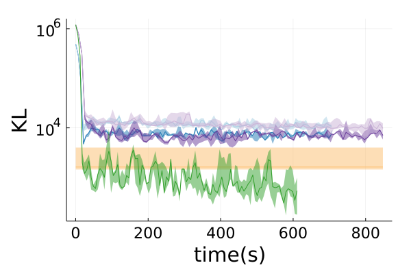
(a) (a)

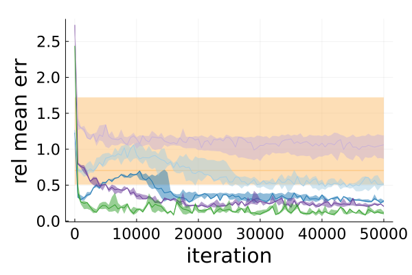
(b) (b)

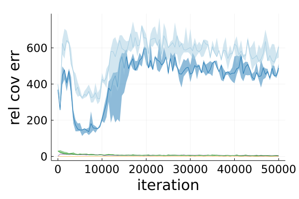
(c) (c)

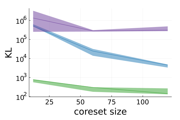
(d) (d)

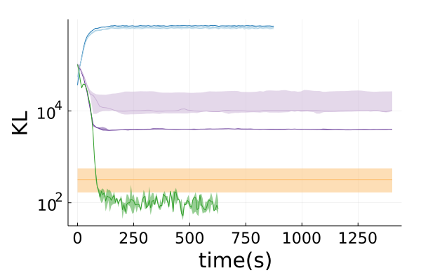
(e) (e)

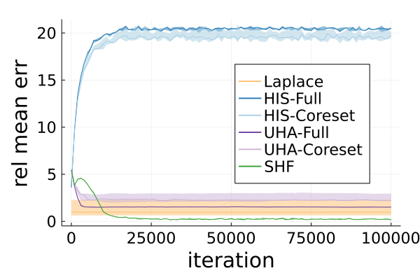
(f) (f)

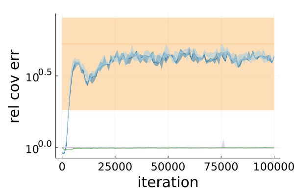
(g) (g)

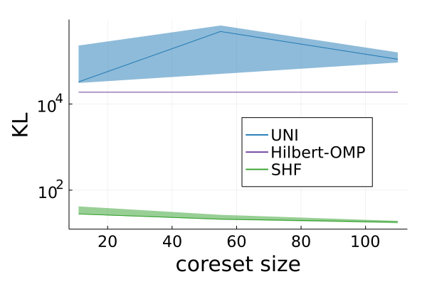
(h) (h)

Figure 5: Linear (top) and logistic (bottom) regression results: Gaussian approximated KL divergence versus training time (Figs. 5(a) and 5(e)), relative 2-norm mean error (Figs. 5(b) and 5(f)), relative Frobenius norm covariance error (Figs. 5(c) and 5(g)), and Gaussian approximated KL divergence versus coreset size (Figs. 5(d) and 5(h)). The lines indicate the median, and error regions indicate 25${}^{\text{th}}$ to 75${}^{\text{th}}$ percentile from 5 runs.

4.3 Bayesian logistic regression

In the setting of Bayesian logistic regression, we are given a set of data points $(x_{n},y_{n})^{N}_{n=1}$, each consisting of features $x_{n}\in\mathbb{R}^{p}$ and label $y_{n}\in\{0,1\}$, and a model of the form

$$\forall i\in[p+1],\,\,\beta_{i}\overset{\textrm{\tiny{i.i.d.}\@}}{\sim}{\sf{Cauchy}}(0,1),\quad\forall n\in[N],\,\,y_{n}\overset{\textrm{\tiny{indep}}}{\sim}{\sf{Bern}}\left(\left(1+\exp\left(-\begin{bmatrix}1&x_{n}^{T}\end{bmatrix}\beta\right)\right)^{-1}\right),\addcontentsline{lla}{section}{\numberline{\string\crtrefnumber{eq:logreg_model}}{e}q:logreg_{m}odel}$$ (21)

where $\beta\in\mathbb{R}^{p+1}$. The same airline dataset is used with the labels indicating whether a flight is cancelled. Of the flights included, $1.384\%$ were cancelled. More details can be found in Section B.3.

The same procedures as in the Bayesian linear regression example are followed to generate the results in Figs. 5(e), 5(f), 5(g) and 5(h). To account for the class imbalance problem present in the dataset, we construct all subsampled coresets with half the data having label $1$ and the rest with label $0$. The results in Figs. 5(e), 5(f), 5(g) and 5(h) are similar to those from the Bayesian linear regression example; SHF provides high quality variational approximations to the posterior. Additional plots comparing the quality of posterior approximations using various other metrics can be found in Section B.3.

5 Conclusion

This paper introduced sparse Hamiltonian flows, a novel coreset-based variational family that enables tractable i.i.d. sampling, and evalution of density and normalization constant. The method randomly subsamples a small set of data, and uses the subsample to construct a flow from sparse Hamiltonian dynamics. Novel quasi-refreshment steps provide the flow with the flexibility to match target posteriors without introducing additional auxiliary variables. Theoretical results show that, in a representative model, the method can recover the exact posterior using a subsampled dataset of the size that is a logarithm of its original size, and that quasi-refreshments are guaranteed to reduce the KL divergence to the target. Experiments demonstrate that the method provides high quality coreset posterior approximations. One main limitation of our methodology is that the data must be “compressible" in the sense that log-likelihood functions of a subset can be used to well represent the full log-likelihood. If the data do not live on some underlying low-dimensional manifold, this may not be the case. Additionally, while our quasi-refreshment is simple and works well in practice, more work is required to develop a wider variety of general-purpose quasi-refreshment moves. We leave this for future work.

Checklist

1. For all authors…

   1. Do the main claims made in the abstract and introduction accurately reflect the paper’s contributions and scope? [Yes]

   2. Did you describe the limitations of your work? [Yes] In Section 3.3, we assume that the momentum distribution is Gaussian. In Section 5, we mention that a direction of future work is to develop more general quasi-refreshment moves that do not require such assumptions.

   3. Did you discuss any potential negative societal impacts of your work? [No] This paper presents an algorithm for sampling from a Bayesian posterior distribution in the large-scale data regime. There are possible negative societal impacts of downstream applications of this method (e.g. inference for a particular model and dataset), but we prefer not to speculate about these here.

   4. Have you read the ethics review guidelines and ensured that your paper conforms to them? [Yes]

2. If you are including theoretical results…

   1. Did you state the full set of assumptions of all theoretical results? [Yes]

   2. Did you include complete proofs of all theoretical results? [Yes] All proofs are provided in the appendix

3. If you ran experiments…

   1. Did you include the code, data, and instructions needed to reproduce the main experimental results (either in the supplemental material or as a URL)? [Yes] We have included anonymized code in the supplement.

   2. Did you specify all the training details (e.g., data splits, hyperparameters, how they were chosen)? [Yes] All details are provided in the main paper and in Appendix B.

   3. Did you report error bars (e.g., with respect to the random seed after running experiments multiple times)? [Yes] All results come with error bars.

   4. Did you include the total amount of compute and the type of resources used (e.g., type of GPUs, internal cluster, or cloud provider)? [Yes] Hardware is listed at the beginning of the experiments.

4. If you are using existing assets (e.g., code, data, models) or curating/releasing new assets…

   1. If your work uses existing assets, did you cite the creators? [Yes] Footnotes to the source URL and bibliography citations are provided.

   2. Did you mention the license of the assets? [No] None of the real datasets we use specify a particular license that the data were released under.

   3. Did you include any new assets either in the supplemental material or as a URL? [N/A] We do not produce any new assets.

   4. Did you discuss whether and how consent was obtained from people whose data you’re using/curating? [No] Our data does not pertain to individuals.

   5. Did you discuss whether the data you are using/curating contains personally identifiable information or offensive content? [No] Our data does not pertain to individuals.

5. If you used crowdsourcing or conducted research with human subjects…

   1. Did you include the full text of instructions given to participants and screenshots, if applicable? [N/A]

   2. Did you describe any potential participant risks, with links to Institutional Review Board (IRB) approvals, if applicable? [N/A]

   3. Did you include the estimated hourly wage paid to participants and the total amount spent on participant compensation? [N/A]

Appendix A Additional details on quasi-refreshment

In this section, we extend marginal quasi-refreshment beyond what is discussed in the main text and introduce conditional quasi-refreshment, which tries to match some conditional distribution of $(\rho_{t},\theta_{t})$ to that corresponding distribution in the target.

Marginal quasi-refreshment

We begin by presenting a more general version of Proposition 3.3.

Proposition A.1.

Consider random vectors $Y,Z,Y^{\prime},Z^{\prime}\in\mathbb{R}^{d}$ for some $d\in\mathbb{N}$. Suppose that $Y\mathchoice{\mathrel{\hbox to0.0pt{$\displaystyle\perp$\hss}\mkern 4.0mu{\displaystyle\perp}}}{\mathrel{\hbox to0.0pt{$\textstyle\perp$\hss}\mkern 4.0mu{\textstyle\perp}}}{\mathrel{\hbox to0.0pt{$\scriptstyle\perp$\hss}\mkern 4.0mu{\scriptstyle\perp}}}{\mathrel{\hbox to0.0pt{$\scriptscriptstyle\perp$\hss}\mkern 4.0mu{\scriptscriptstyle\perp}}}Z$ and that we have a bijection $R:\mathbb{R}^{d}\to\mathbb{R}^{d}$ such that $R(Y^{\prime})\overset{d}{=}Y$. Then

$$\mathrm{D_{KL}}\mathchoice{\left({{{{R(Y^{\prime}),Z^{\prime}||Y,Z}}}}\right)}{({{{{R(Y^{\prime}),Z^{\prime}||Y,Z}}}})}{({{{{R(Y^{\prime}),Z^{\prime}||Y,Z}}}})}{({{{{R(Y^{\prime}),Z^{\prime}||Y,Z}}}})} =\mathrm{D_{KL}}\mathchoice{\left({{{{Y^{\prime},Z^{\prime}||Y,Z}}}}\right)}{({{{{Y^{\prime},Z^{\prime}||Y,Z}}}})}{({{{{Y^{\prime},Z^{\prime}||Y,Z}}}})}{({{{{Y^{\prime},Z^{\prime}||Y,Z}}}})}-\mathrm{D_{KL}}\mathchoice{\left({{{{Y^{\prime}||Y}}}}\right)}{({{{{Y^{\prime}||Y}}}})}{({{{{Y^{\prime}||Y}}}})}{({{{{Y^{\prime}||Y}}}})}.$$ (22)

Proof.

Since $R$ is a bijection,

$$\mathrm{D_{KL}}\mathchoice{\left({{{{R(Y^{\prime}),Z^{\prime}||Y,Z}}}}\right)}{({{{{R(Y^{\prime}),Z^{\prime}||Y,Z}}}})}{({{{{R(Y^{\prime}),Z^{\prime}||Y,Z}}}})}{({{{{R(Y^{\prime}),Z^{\prime}||Y,Z}}}})} =\mathrm{D_{KL}}\mathchoice{\left({{{{Y^{\prime},Z^{\prime}||R^{-1}(Y),Z}}}}\right)}{({{{{Y^{\prime},Z^{\prime}||R^{-1}(Y),Z}}}})}{({{{{Y^{\prime},Z^{\prime}||R^{-1}(Y),Z}}}})}{({{{{Y^{\prime},Z^{\prime}||R^{-1}(Y),Z}}}})}.$$ (23)

Because $Y\mathchoice{\mathrel{\hbox to0.0pt{$\displaystyle\perp$\hss}\mkern 4.0mu{\displaystyle\perp}}}{\mathrel{\hbox to0.0pt{$\textstyle\perp$\hss}\mkern 4.0mu{\textstyle\perp}}}{\mathrel{\hbox to0.0pt{$\scriptstyle\perp$\hss}\mkern 4.0mu{\scriptstyle\perp}}}{\mathrel{\hbox to0.0pt{$\scriptscriptstyle\perp$\hss}\mkern 4.0mu{\scriptscriptstyle\perp}}}Z$, and $R(Y^{\prime})\overset{d}{=}Y$,

$$\mathrm{D_{KL}}\mathchoice{\left({{{{Y^{\prime},Z^{\prime}||R^{-1}(Y),Z}}}}\right)}{({{{{Y^{\prime},Z^{\prime}||R^{-1}(Y),Z}}}})}{({{{{Y^{\prime},Z^{\prime}||R^{-1}(Y),Z}}}})}{({{{{Y^{\prime},Z^{\prime}||R^{-1}(Y),Z}}}})} =\mathrm{D_{KL}}\mathchoice{\left({{{{Y^{\prime}||R^{-1}(Y)}}}}\right)}{({{{{Y^{\prime}||R^{-1}(Y)}}}})}{({{{{Y^{\prime}||R^{-1}(Y)}}}})}{({{{{Y^{\prime}||R^{-1}(Y)}}}})}+\mathbb{E}\left[\mathrm{D_{KL}}\mathchoice{\left({{{{(Z^{\prime}|Y^{\prime})||Z}}}}\right)}{({{{{(Z^{\prime}|Y^{\prime})||Z}}}})}{({{{{(Z^{\prime}|Y^{\prime})||Z}}}})}{({{{{(Z^{\prime}|Y^{\prime})||Z}}}})}\right]$$ (24)

$$=\mathbb{E}\left[\mathrm{D_{KL}}\mathchoice{\left({{{{(Z^{\prime}|Y^{\prime})||Z}}}}\right)}{({{{{(Z^{\prime}|Y^{\prime})||Z}}}})}{({{{{(Z^{\prime}|Y^{\prime})||Z}}}})}{({{{{(Z^{\prime}|Y^{\prime})||Z}}}})}\right].$$ (25)

Then we add and subtract $\mathrm{D_{KL}}\mathchoice{\left({{{{Y^{\prime}||Y}}}}\right)}{({{{{Y^{\prime}||Y}}}})}{({{{{Y^{\prime}||Y}}}})}{({{{{Y^{\prime}||Y}}}})}$ to obtain the final result,

$$\mathbb{E}\left[\mathrm{D_{KL}}\mathchoice{\left({{{{(Z^{\prime}|Y^{\prime})||Z}}}}\right)}{({{{{(Z^{\prime}|Y^{\prime})||Z}}}})}{({{{{(Z^{\prime}|Y^{\prime})||Z}}}})}{({{{{(Z^{\prime}|Y^{\prime})||Z}}}})}\right] =\mathrm{D_{KL}}\mathchoice{\left({{{{Y^{\prime},Z^{\prime}||Y,Z}}}}\right)}{({{{{Y^{\prime},Z^{\prime}||Y,Z}}}})}{({{{{Y^{\prime},Z^{\prime}||Y,Z}}}})}{({{{{Y^{\prime},Z^{\prime}||Y,Z}}}})}-\mathrm{D_{KL}}\mathchoice{\left({{{{Y^{\prime}||Y}}}}\right)}{({{{{Y^{\prime}||Y}}}})}{({{{{Y^{\prime}||Y}}}})}{({{{{Y^{\prime}||Y}}}})}.$$ (26)

∎

Then Proposition 3.3 follows immediately from Proposition A.1.

Proof of Proposition 3.3.

By setting $Y=\rho,Z=\theta,Y^{\prime}=\rho_{t}$, and $Z^{\prime}=\theta_{t}$, we arrive at the stated result. ∎

More generally, in order to apply Proposition A.1, we first need to split the momentum variable into two components $(\rho^{(1)},\rho^{(2)})$ in such a way that $\rho^{(1)}\mathchoice{\mathrel{\hbox to0.0pt{$\displaystyle\perp$\hss}\mkern 4.0mu{\displaystyle\perp}}}{\mathrel{\hbox to0.0pt{$\textstyle\perp$\hss}\mkern 4.0mu{\textstyle\perp}}}{\mathrel{\hbox to0.0pt{$\scriptstyle\perp$\hss}\mkern 4.0mu{\scriptstyle\perp}}}{\mathrel{\hbox to0.0pt{$\scriptscriptstyle\perp$\hss}\mkern 4.0mu{\scriptscriptstyle\perp}}}\rho^{(2)}$ under $(\theta,\rho)\sim\bar{\pi}$, and then set $Y=\rho^{(1)}$ and $Z=(\rho^{(2)},\theta)$. Since we know that $\rho\sim\mathcal{N}(0,I)$, we have quite a few options. For example:

• Set $Y=\rho$, and $Z=\theta$. Then

  $$Y\mathchoice{\mathrel{\hbox to0.0pt{$\displaystyle\perp$\hss}\mkern 4.0mu{\displaystyle\perp}}}{\mathrel{\hbox to0.0pt{$\textstyle\perp$\hss}\mkern 4.0mu{\textstyle\perp}}}{\mathrel{\hbox to0.0pt{$\scriptstyle\perp$\hss}\mkern 4.0mu{\scriptstyle\perp}}}{\mathrel{\hbox to0.0pt{$\scriptscriptstyle\perp$\hss}\mkern 4.0mu{\scriptscriptstyle\perp}}}Z\quad\text{and}\quad Y\sim\mathcal{N}(0,I).$$ (27)

• Set $Y=\|D\rho\|^{2}_{2}$ and $Z=\left(\frac{D\rho}{\|D\rho\|_{2}},(I-D)\rho,\theta\right)$ for any binary diagonal matrix $D\in\mathbb{R}^{d\times d}$. Then

  $$Y\mathchoice{\mathrel{\hbox to0.0pt{$\displaystyle\perp$\hss}\mkern 4.0mu{\displaystyle\perp}}}{\mathrel{\hbox to0.0pt{$\textstyle\perp$\hss}\mkern 4.0mu{\textstyle\perp}}}{\mathrel{\hbox to0.0pt{$\scriptstyle\perp$\hss}\mkern 4.0mu{\scriptstyle\perp}}}{\mathrel{\hbox to0.0pt{$\scriptscriptstyle\perp$\hss}\mkern 4.0mu{\scriptscriptstyle\perp}}}Z\quad\text{and}\quad Y\sim\chi^{2}(\operatorname{tr}D).$$ (28)

• Set $Y=a^{T}\rho$ for any $a\in\mathbb{R}^{d}$ such that $\|a\|=1$, and $Z=\left((I-aa^{T})\rho,\theta\right)$. Then

  $$Y\mathchoice{\mathrel{\hbox to0.0pt{$\displaystyle\perp$\hss}\mkern 4.0mu{\displaystyle\perp}}}{\mathrel{\hbox to0.0pt{$\textstyle\perp$\hss}\mkern 4.0mu{\textstyle\perp}}}{\mathrel{\hbox to0.0pt{$\scriptstyle\perp$\hss}\mkern 4.0mu{\scriptstyle\perp}}}{\mathrel{\hbox to0.0pt{$\scriptscriptstyle\perp$\hss}\mkern 4.0mu{\scriptscriptstyle\perp}}}Z\quad\text{and}\quad Y\sim\mathcal{N}(0,1).$$ (29)

Note again that the first option recovers the marginal quasi-refreshment in the main text. Now we use the above decomposition to design a marginal quasi-refreshment move. Suppose we have run the weighted sparse leapfrog integrator Eq. 14 up to time $t$, resulting in a current random state $\theta_{t},\rho_{t}$. Let the decomposition of the current state $(\theta_{t},\rho_{t})$ that we select above be denoted $Y^{\prime},Z^{\prime}$. Then the marginal quasi-refreshment move involves finding a map $R$ such that $R(Y^{\prime})\overset{d}{=}Y$. We can then refresh the state via $(R(Y^{\prime}),Z^{\prime})$, and continue the flow. In addition to the parametric approach to designing $R$ presented in the main text, if $Y$ is 1-dimensional—for example, if we are trying to refresh the momentum norm $Y=\|\rho\|_{2}$—then given that we know the CDF $F$ of $Y$, we can estimate the CDF $\hat{F}$ of $Y^{\prime}$ using samples from the flow at timestep $t$, and then set

$$R(x)=F^{-1}\left(\hat{F}(x)\right).$$ (30)

For example, we could use this inverse CDF map technique to refresh the distribution of $\|\rho\|^{2}_{2}$ back to $\chi^{2}(d)$, or to refresh the distribution of $a^{T}\rho$ back to $\mathcal{N}(0,1)$.

Conditional quasi-refreshment

A conditional quasi-refreshment move is one that tries to make some conditional distribution of $(\rho_{t},\theta_{t})$ match the same conditional in the target. If one is able to accomplish this for any conditional distribution (with no requirement of independence as in the marginal case), the KL divergence is guaranteed to reduce.

Proposition A.2.

Consider random vectors $Y,Z,Y^{\prime},Z^{\prime}\in\mathbb{R}^{d}$ for some $d\in\mathbb{N}$. Suppose for each $s\in\mathbb{R}^{d}$ we have a bijection $R_{s}:\mathbb{R}^{d}\to\mathbb{R}^{d}$ such that $(R_{s}(Y^{\prime})\mid Z^{\prime}=s)\overset{d}{=}(Y\mid Z=s)$. Then

$$\mathrm{D_{KL}}\mathchoice{\left({{{{R_{Z^{\prime}}(Y^{\prime}),Z^{\prime}||Y,Z}}}}\right)}{({{{{R_{Z^{\prime}}(Y^{\prime}),Z^{\prime}||Y,Z}}}})}{({{{{R_{Z^{\prime}}(Y^{\prime}),Z^{\prime}||Y,Z}}}})}{({{{{R_{Z^{\prime}}(Y^{\prime}),Z^{\prime}||Y,Z}}}})} =\mathrm{D_{KL}}\mathchoice{\left({{{{Z^{\prime}||Z}}}}\right)}{({{{{Z^{\prime}||Z}}}})}{({{{{Z^{\prime}||Z}}}})}{({{{{Z^{\prime}||Z}}}})}.$$ (31)

Proof.

By assumption the distribution of $Y$ given $Z=s$ is the same as that of $R_{s}(Y^{\prime})$ given $Z^{\prime}=s$; so the result follows directly from the decomposition

$$\mathrm{D_{KL}}\mathchoice{\left({{{{R_{Z^{\prime}}(Y^{\prime}),Z^{\prime}||Y,Z}}}}\right)}{({{{{R_{Z^{\prime}}(Y^{\prime}),Z^{\prime}||Y,Z}}}})}{({{{{R_{Z^{\prime}}(Y^{\prime}),Z^{\prime}||Y,Z}}}})}{({{{{R_{Z^{\prime}}(Y^{\prime}),Z^{\prime}||Y,Z}}}})} =\mathrm{D_{KL}}\mathchoice{\left({{{{Z^{\prime}||Z}}}}\right)}{({{{{Z^{\prime}||Z}}}})}{({{{{Z^{\prime}||Z}}}})}{({{{{Z^{\prime}||Z}}}})}+\mathbb{E}\left[\mathrm{D_{KL}}\mathchoice{\left({{{{(R_{S}(Y^{\prime})|Z^{\prime}=S)||(Y|Z=S)}}}}\right)}{({{{{(R_{S}(Y^{\prime})|Z^{\prime}=S)||(Y|Z=S)}}}})}{({{{{(R_{S}(Y^{\prime})|Z^{\prime}=S)||(Y|Z=S)}}}})}{({{{{(R_{S}(Y^{\prime})|Z^{\prime}=S)||(Y|Z=S)}}}})}\right],\quad S\overset{d}{=}Z^{\prime}$$ (32)

$$=\mathrm{D_{KL}}\mathchoice{\left({{{{Z^{\prime}||Z}}}}\right)}{({{{{Z^{\prime}||Z}}}})}{({{{{Z^{\prime}||Z}}}})}{({{{{Z^{\prime}||Z}}}})}.$$ (33)

∎

Conditional moves are much harder to design than marginal moves in general. One case of particular utility occurs when one is willing to assume that $(\theta_{t},\rho_{t})$ are roughly jointly normally distributed. In this case,

$$\begin{bmatrix}\theta_{t}\\ \rho_{t}\end{bmatrix}\sim\mathcal{N}\left(\begin{bmatrix}\mu_{\theta}\\ \mu_{\rho}\end{bmatrix},\begin{bmatrix}\Sigma_{\theta\theta}&\Sigma_{\theta\rho}\\ \Sigma_{\theta\rho}^{T}&\Sigma_{\rho\rho}\end{bmatrix}\right),$$ (34)

so one can refresh the momentum $\rho_{t}$ by updating it to $R_{\theta_{t}}(\rho_{t})$, where

$$R_{s}(x)=\Sigma^{-1/2}\left(x-\mu_{\rho}-\Sigma_{\theta\rho}^{T}\Sigma_{\theta\theta}^{-1}\left(s-\mu_{\theta}\right)\right)\quad\text{and}\quad\Sigma=\Sigma_{\rho\rho}-\Sigma_{\theta\rho}^{T}\Sigma_{\theta\theta}^{-1}\Sigma_{\theta\rho}.$$ (35)

Here Proposition A.2 applies by setting $Y=\rho,Z=\theta,Y^{\prime}=\rho_{t}$, and $Z^{\prime}=\theta_{t}$. In order to use this quasi-refreshment move, one can either include the covariance matrices and mean vectors as tunable parameters in the optimization, or use samples from the flow at step $t$ to estimate them directly.

Appendix B Details of experiments

We begin by describing in detail the differences between HIS-Full/UHA-Full and HIS-Coreset/UHA-Coreset. It is worth noting noting that we were unable to train HIS/UHA with full-dataset flow dynamics; even on a small 2-dimensional Gaussian location model with 100 data points, these methods took over 8 minutes for training. Therefore, as suggested by [21, 23], we train the leapfrog step sizes and annealing parameters by using a random minibatch of the data in each iteration to construct the flow dynamics. To then obtain valid ELBO estimates for comparison, we generate samples from the trained flow with leapfrog transformations based on the full dataset (HIS-Full/UHA-Full). As a simple heuristic baseline that also provides a valid ELBO estimate, we compare to the trained flow with leapfrog transformations based on a fixed, uniformly sampled coreset (HIS-Coreset/UHA-Coreset) of the same size as used for SHF.

We now describe the detailed settings that apply across all three experiments in the main text. In all experiments, SHF uses the quasi-refreshment from Eq. 18 initialized using the warm-start procedure in Section 3 with a batch of $100$ samples. We use the same number of leapfrog, tempering, and (quasi-)refreshment steps for all of SHF, HIS and UHA respectively. The leapfrog step sizes are initialized at the same value for all three methods. For all three methods (SHF, HIS, and UHA), the unnormalized log target density used in computing the ELBO objective is estimated using a minibatch of $S=100$ data points for each optimization iteration. For both HIS and UHA, the leapfrog transitions themselves are also based on a fresh uniformly sampled minibatch of size 30—the same as the coreset size for SHF—at each optimization iteration. HIS and UHA both also involve tempering procedures, requiring optimization over the tempering schedule $0\leq\beta_{1}\leq\dots\leq\beta_{R-1}\leq\beta_{R}=1$, where $R$ denotes the number of tempering steps (equal to the number of quasi-refreshment / refreshment steps in all methods). We consider a reparameterization of $(\beta_{1},\dots,\beta_{R})$ to $(\alpha_{1},\dots,\alpha_{R-1})$, where $\alpha_{r}=\text{Logit}(\beta_{r+1}/\beta_{r})$ for $r\in\{1,\dots,R-1\}$, ensuring a set of unconstrained parameters. The initial value for each $r$ is set to $\alpha_{r}=1$. For UHA, the initial damping coefficient of its partial momentum refreshment is set to $0.5$. We estimate all evaluation metrics using $100$ samples. To estimate KSD, we use the IMQ base kernel with its parameters set to the same values as outlined in [45] ($\beta=-\frac{1}{2}$ and $c=1$).

In addition to HIS and UHA, we also include adaptive HMC and NUTS in our comparison of density evaluation and sample generation times. We tune adaptive HMC and NUTS with a target acceptance rate of $0.65$ during a number of burn-in iterations equal to the number of output samples, and include the burn-in time in the timing results for these two methods. Finally, we compare the quality of coresets constructed by SHF against UNI and Hilbert-OMP. For both UNI and Hilbert-OMP, we use NUTS to draw samples from the coreset posterior approximation. For Hilbert-OMP, we use a random log-likelihood function projection of dimension $100d$, where the true posterior parameter is of dimension $d$, generated from the Laplace approximation [47].

B.1 Synthetic Gaussian

To train SHF, a total of 5 quasi-refreshments are used with 10 leapfrog steps in between; a similar schedule is used in HIS and UHA for momentum tempering and refreshment respectively. The initial distribution is set to $\theta_{0}\sim\mathcal{N}(0,I)$ and $\rho_{0}\sim\mathcal{N}(0,I)$. For all methods, the number of optimization iterations is set to $20,000$, and the initial leapfrog step size is set to $0.01$ across all $d$ dimensions. We train all methods with ADAM with initial learning rate $0.001$.

B.2 Bayesian linear regression

To train SHF, a total of 8 quasi-refreshments are used with 10 leapfrog steps in between; a similar schedule is used in HIS and UHA for momentum tempering and refreshment respectively. The initial distribution is set to $\theta_{0}\sim\mathcal{N}(15,0.01I)$ and $\rho_{0}\sim\mathcal{N}(0,I)$. For all methods, the number of optimization iterations is set to $50,000$, and the initial leapfrog step size is set to $0.02$ across all $d$ dimensions except for the dimension for the $\log\sigma^{2}$ term, where the step size is set to $0.0002$. We train all methods with ADAM with initial learning rate $0.002$. We also include the posterior approximation obtained from the Laplace approximation, where we search for the mode of the target density at some location generated from the same distribution as that of $\theta_{0}$. Figs. 6, 8 and 7 provide additional results for this experiment. Fig. 6(a) shows that the ELBO obtained from SHF is a tighter lower bound of the log normalization constant compared to HIS and UHA. Fig. 6(b) shows that SHF produces a posterior approximation in terms of energy distance than all other methods; Fig. 6(c) shows that SHF is competitive, if not better, than the other methods in terms of KSD. Figs. 7(a), 7(b), 7(c) and 7(d) show that the coreset constructed by SHF is of better quality than those obtained from UNI and Hilbert-OMP in terms of all four metrics shown. Finally, Figs. 8(a) and 8(b) show the computational gain of using SHF to approximate density and generate posterior samples as compared to HIS and UHA.

B.3 Bayesian logistic regression

To train SHF, a total of 8 quasi-refreshments are used with 10 leapfrog steps in between; a similar schedule is used in HIS and UHA for momentum tempering and refreshment respectively. The initial distribution is set to $\theta_{0}\sim\mathcal{N}(15,10^{-4}I)$ and $\rho_{0}\sim\mathcal{N}(0,I)$. For all methods, the number of optimization iterations is set to $100,000$, and the initial leapfrog step size is set to $0.0005$ across all $d$ dimensions. We train all methods with ADAM with initial learning rate $0.001$. We also include the posterior approximation obtained from the Laplace approximation, where we search for the mode of the target density at some location generated from the same distribution as that of $\theta_{0}$. Figs. 6, 7 and 8 provide additional results for this experiment, where similar conclusions as in the Bayesian linear regression experiment can be drawn.

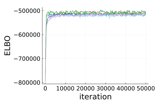
(a) (a)

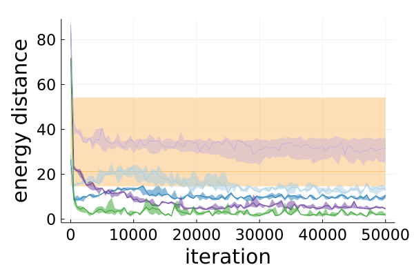
(b) (b)

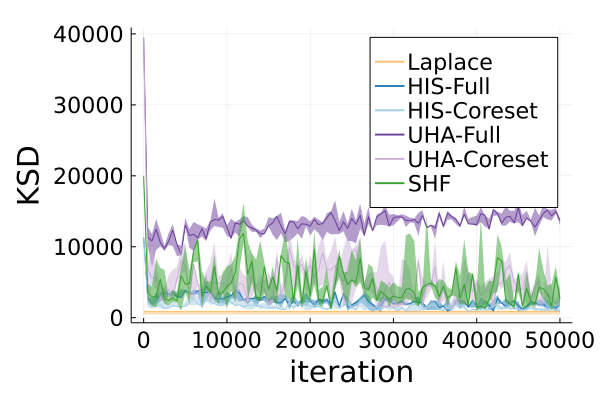
(c) (c)

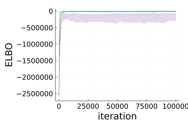
(d) (d)

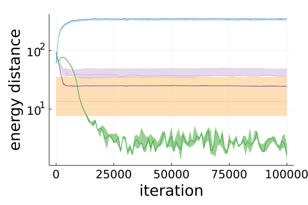
(e) (e)

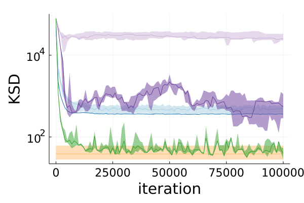
(f) (f)

Figure 6: Linear (top row, Figs. 6(a), 6(b) and 6(c)) and logistic (bottom row Figs. 6(d), 6(e) and 6(f)) regression: posterior approximation quality results. The lines indicate the median, and error regions indicate 25${}^{\text{th}}$ to 75${}^{\text{th}}$ percentile from 5 runs.

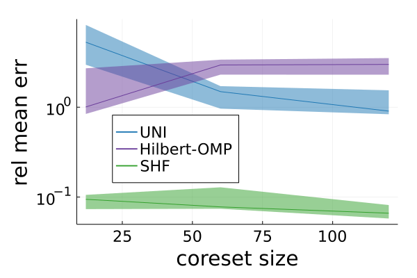
(a) (a)

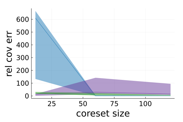
(b) (a)

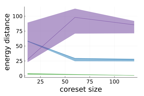
(c) (a)

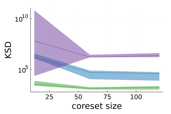
(d) (a)

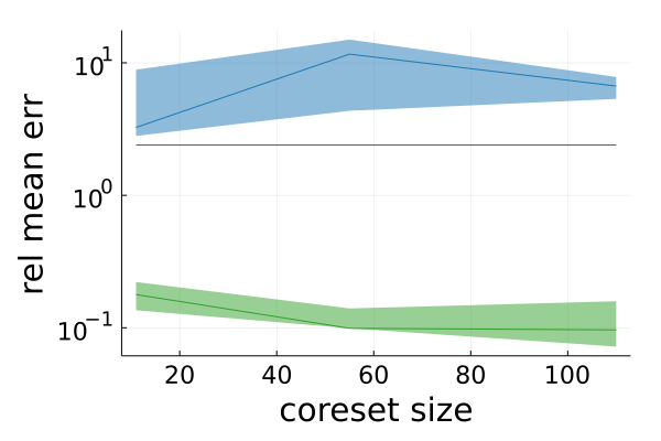
(e) (a)

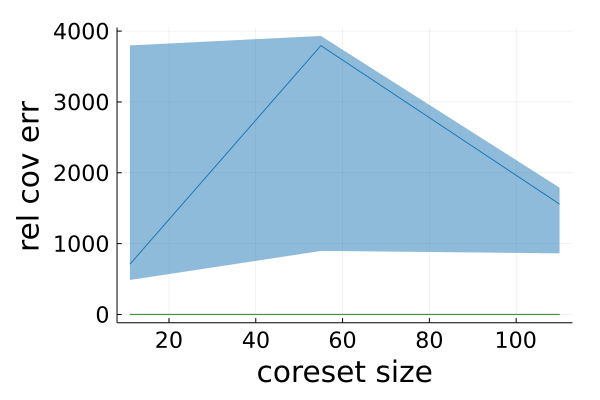
(f) (a)

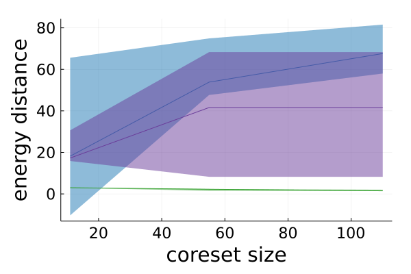
(g) (a)

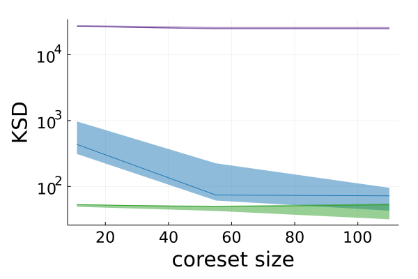
(h) (a)

Figure 7: Linear (top row, Figs. 7(a), 7(b), 7(c) and 7(d)) and logistic (bottom row Figs. 7(e), 7(f), 7(g) and 7(h)) regression: posterior approximation quality results. The lines indicate the median, and error regions indicate 25${}^{\text{th}}$ to 75${}^{\text{th}}$ percentile from 5 runs.

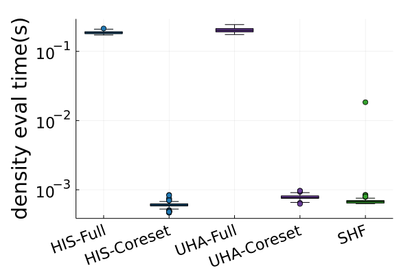
(a) (a)

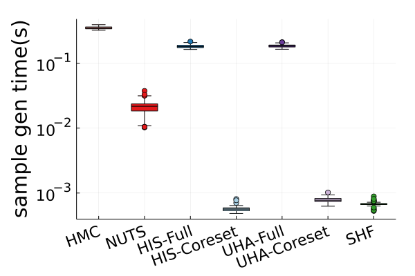
(b) (b)

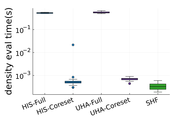
(c) (c)

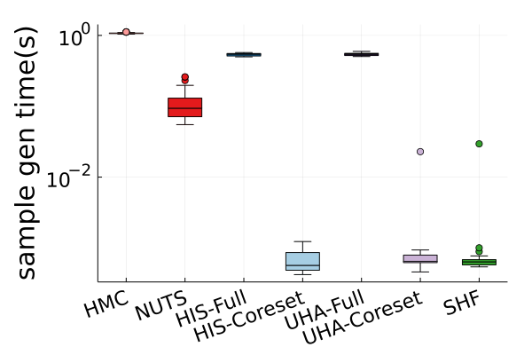
(d) (d)

Figure 8: Linear (Figs. 8(a) and 8(b)) and logistic (Figs. 8(c) and 8(d)) regression: timing results based on 100 samples.

Appendix C Gaussian KL upper bound proof

Proof of Proposition 3.1.

Suppose we are given a particular choice $\mathcal{I}\subseteq[N]$ of $N$ indices of size $|\mathcal{I}|=M\in\mathbb{N}$, $M\leq N$. Let $\mathcal{W}_{\mathcal{I}}=\left\{w\in\mathbb{R}_{+}^{N}:\forall n\in[N],n\notin\mathcal{I}\implies w_{n}=0\right\}$. In the $d$-dimensional normal location model, the exact and $w\in\mathcal{W}_{\mathcal{I}}$-coreset posteriors are multivariate Gaussian distributions, denoted as $\mathcal{N}{\left(\mu_{1},\Sigma_{1}\right)}$ and $\mathcal{N}{\left(\mu_{w},\Sigma_{w}\right)}$ respectively, with mean and covariance

$$\Sigma_{1}=\frac{1}{1+N}I,\quad\mu_{1}=\Sigma_{1}\left(\sum_{n=1}^{N}X_{n}\right)\quad\text{and}\quad\Sigma_{w}\!=\!\frac{I}{1+\left(\sum_{n\in\mathcal{I}}w_{n}\right)},\quad\mu_{w}\!=\!\Sigma_{w}\left(\sum_{n\in\mathcal{I}}w_{n}X_{n}\right).\addcontentsline{lla}{section}{\numberline{\string\crtrefnumber{eq:gauss_posts}}{e}q:gauss_{p}osts}$$ (36)

The KL divergence between these two distributions is

$$\mathrm{D_{KL}}\mathchoice{\left({{{{\pi_{w}||\pi}}}}\right)}{({{{{\pi_{w}||\pi}}}})}{({{{{\pi_{w}||\pi}}}})}{({{{{\pi_{w}||\pi}}}})}= \frac{1}{2}\left[-d\log\left(\frac{1+N}{1+\sum_{n\in\mathcal{I}}w_{n}}\right)-d+d\left(\frac{1+N}{1+\sum_{n\in\mathcal{I}}w_{n}}\right)+(\mu_{1}-\mu_{w})^{T}\Sigma_{1}^{-1}(\mu_{1}-\mu_{w})\right].\addcontentsline{lla}{section}{\numberline{\string\crtrefnumber{eq:KL_from_coreset_post_to_exact}}{e}q:KL_{f}rom_{c}oreset_{p}ost_{t}o_{e}xact}$$ (37)

We can bound this quantity above by adding the constraint $\sum_{n\in\mathcal{I}}w_{n}=N$, yielding

$$\min_{w\in\mathcal{W}_{\mathcal{I}}}\mathrm{D_{KL}}\mathchoice{\left({{{{\pi_{w}||\pi}}}}\right)}{({{{{\pi_{w}||\pi}}}})}{({{{{\pi_{w}||\pi}}}})}{({{{{\pi_{w}||\pi}}}})}\leq\min_{w\in\triangle^{M-1}}\frac{N^{2}}{2(N+1)}\left\|\bar{X}-\sum_{n\in\mathcal{I}}w_{n}X_{n}\right\|^{2},$$ (38)

where $\bar{X}=\frac{1}{N}\sum_{n=1}^{N}X_{n}$. and $\triangle^{M-1}$ is the $M-1$-dimensional simplex $w\geq 0$, $1^{T}w=1$. We aim to show that with high probability (over uniform random choice of $\mathcal{I}$ and realizations of $X_{n},n\in[N]$), there exists a $w\in\triangle^{M-1}$ such that $\bar{X}=\sum_{n\in\mathcal{I}}w_{n}X_{n}$, and hence the optimal KL divergence is 0.

Since $X_{n}\overset{\textrm{\tiny{i.i.d.}\@}}{\sim}\mathcal{N}(0,I)$, $\mathchoice{{\hbox{$\displaystyle\sqrt{N\,}$}\lower 0.4pt\hbox{\vrule height=6.14998pt,depth=-4.92001pt}}}{{\hbox{$\textstyle\sqrt{N\,}$}\lower 0.4pt\hbox{\vrule height=6.14998pt,depth=-4.92001pt}}}{{\hbox{$\scriptstyle\sqrt{N\,}$}\lower 0.4pt\hbox{\vrule height=4.305pt,depth=-3.44402pt}}}{{\hbox{$\scriptscriptstyle\sqrt{N\,}$}\lower 0.4pt\hbox{\vrule height=3.07498pt,depth=-2.46pt}}}\bar{X}\sim\mathcal{N}(0,I)$, so $\|\mathchoice{{\hbox{$\displaystyle\sqrt{N\,}$}\lower 0.4pt\hbox{\vrule height=6.14998pt,depth=-4.92001pt}}}{{\hbox{$\textstyle\sqrt{N\,}$}\lower 0.4pt\hbox{\vrule height=6.14998pt,depth=-4.92001pt}}}{{\hbox{$\scriptstyle\sqrt{N\,}$}\lower 0.4pt\hbox{\vrule height=4.305pt,depth=-3.44402pt}}}{{\hbox{$\scriptscriptstyle\sqrt{N\,}$}\lower 0.4pt\hbox{\vrule height=3.07498pt,depth=-2.46pt}}}\bar{X}\|^{2}\sim\chi^{2}(d)$ and therefore for any $s>\mathchoice{{\hbox{$\displaystyle\sqrt{d/N\,}$}\lower 0.4pt\hbox{\vrule height=6.75pt,depth=-5.40002pt}}}{{\hbox{$\textstyle\sqrt{d/N\,}$}\lower 0.4pt\hbox{\vrule height=6.75pt,depth=-5.40002pt}}}{{\hbox{$\scriptstyle\sqrt{d/N\,}$}\lower 0.4pt\hbox{\vrule height=4.72499pt,depth=-3.78001pt}}}{{\hbox{$\scriptscriptstyle\sqrt{d/N\,}$}\lower 0.4pt\hbox{\vrule height=3.375pt,depth=-2.70001pt}}}$,

$$\mathbb{P}\left(\|\bar{X}\|>s\right) \leq\left(\frac{s^{2}N}{d}e^{1-\frac{s^{2}N}{d}}\right)^{d/2}.\addcontentsline{lla}{section}{\numberline{\string\crtrefnumber{eq:bxbound}}{e}q:bxbound}$$ (39)

In other words, as $N$ increases, we can expect $\bar{X}$ to concentrate around the origin. Therefore as long as the convex hull of $X_{n}$, $n\in\mathcal{I}$ contains a ball of some fixed radius around the origin with high probability, we know that $\bar{X}$ is a convex combination of $X_{n},n\in\mathcal{I}$. The radius of the largest origin-centered ball inside the convex hull of $X_{n},n\in\mathcal{I}$ can be expressed as

$$r^{\star} =\min_{a\in\mathbb{R}^{d}:\|a\|=1,b\geq 0}\,b\quad\text{s.t.}\quad\forall n\in\mathcal{I},\quad a^{T}X_{n}-b\leq 0=\min_{a\in\mathbb{R}^{d}:\|a\|=1}\,\max_{n\in\mathcal{I}}\,a^{T}X_{n}.$$ (40)

By Böröczky and Wintsche [37, Corollary 1.2], $S^{d}$ can be covered by

$$N_{d}(\phi)=\frac{C\cdot\cos\phi}{\sin^{d}\phi}d^{\frac{3}{2}}\log(1+d\cos^{2}\phi)\leq\phi^{-d}A_{d},\quad A_{d}=Ce^{\frac{d}{2}}d^{\frac{3}{2}}\log(1+d).\addcontentsline{lla}{section}{\numberline{\string\crtrefnumber{eq:Nphid}}{e}q:Nphid}$$ (41)

balls of radius $0<\phi\leq\arccos\frac{1}{\mathchoice{{\hbox{$\displaystyle\sqrt{d+1\,}$}\lower 0.4pt\hbox{\vrule height=4.375pt,depth=-3.50002pt}}}{{\hbox{$\textstyle\sqrt{d+1\,}$}\lower 0.4pt\hbox{\vrule height=4.375pt,depth=-3.50002pt}}}{{\hbox{$\scriptstyle\sqrt{d+1\,}$}\lower 0.4pt\hbox{\vrule height=3.0625pt,depth=-2.45001pt}}}{{\hbox{$\scriptscriptstyle\sqrt{d+1\,}$}\lower 0.4pt\hbox{\vrule height=2.1875pt,depth=-1.75002pt}}}}$, where $C$ is a universal constant. Denote the centres of these balls $a_{i}\in S^{d}$, $i=1,\dots,N_{d}(\phi)$. Then

$$r^{\star} \geq\min_{i\in[N_{d}(\phi)],v\in\mathbb{R}^{d}:\|v\|\leq\phi}\,\max_{n\in\mathcal{I}}\,(a_{i}+v)^{T}X_{n}$$ (42)

$$\geq\min_{i\in[N_{d}(\phi)]}\,\max_{n\in\mathcal{I}}\,a_{i}^{T}X_{n}-\phi\|X_{n}\|.$$ (43)

Therefore the probability that the largest origin-centred ball enclosed in the convex hull is small is bounded above by

$$\mathbb{P}\left(r^{\star}\leq t\right) \leq\mathbb{P}\left(\min_{i\in[N_{d}(\phi)]}\,\max_{n\in\mathcal{I}}\,a_{i}^{T}X_{n}-\phi\|X_{n}\|\leq t\right)$$ (44)

$$\leq N_{d}(\phi)\mathbb{P}\left(\max_{n\in\mathcal{I}}\,a_{i}^{T}X_{n}-\phi\|X_{n}\|\leq t\right)$$ (45)

$$=N_{d}(\phi)\mathbb{P}\left(a^{T}Z-\phi\|Z\|\leq t\right)^{M},$$ (46)

for $a\in S^{d}$ and $Z\sim\mathcal{N}(0,I)$. Since $Z$ has a spherically symmetric distribution, $a$ is arbitrary, so we can choose $a=\begin{matrix}1&0&\dots&0\end{matrix}^{T}$. If we let $U\sim\mathcal{N}(0,1)$ and $V\sim\chi^{2}(d-1)$ be independent, this yields

$$\mathbb{P}\left(a^{T}Z-\phi\|Z\|\leq t\right) =\mathbb{P}\left(U-\phi\mathchoice{{\hbox{$\displaystyle\sqrt{U^{2}+V\,}$}\lower 0.4pt\hbox{\vrule height=7.77397pt,depth=-6.21921pt}}}{{\hbox{$\textstyle\sqrt{U^{2}+V\,}$}\lower 0.4pt\hbox{\vrule height=7.77397pt,depth=-6.21921pt}}}{{\hbox{$\scriptstyle\sqrt{U^{2}+V\,}$}\lower 0.4pt\hbox{\vrule height=5.465pt,depth=-4.37202pt}}}{{\hbox{$\scriptscriptstyle\sqrt{U^{2}+V\,}$}\lower 0.4pt\hbox{\vrule height=4.23499pt,depth=-3.38802pt}}}\leq t\right)$$ (47)

$$=\mathbb{P}\left(U-t\leq\phi\mathchoice{{\hbox{$\displaystyle\sqrt{U^{2}+V\,}$}\lower 0.4pt\hbox{\vrule height=7.77397pt,depth=-6.21921pt}}}{{\hbox{$\textstyle\sqrt{U^{2}+V\,}$}\lower 0.4pt\hbox{\vrule height=7.77397pt,depth=-6.21921pt}}}{{\hbox{$\scriptstyle\sqrt{U^{2}+V\,}$}\lower 0.4pt\hbox{\vrule height=5.465pt,depth=-4.37202pt}}}{{\hbox{$\scriptscriptstyle\sqrt{U^{2}+V\,}$}\lower 0.4pt\hbox{\vrule height=4.23499pt,depth=-3.38802pt}}}\right)$$ (48)

$$\leq\mathbb{P}\left(U<2t\right)+\mathbb{P}\left(V\geq\phi^{-2}(U-t)^{2}-U^{2},U\geq 2t\right)$$ (49)

$$\leq\Phi(2t)+\mathbb{P}\left(V^{\prime}\geq\phi^{-2}t^{2}\right),$$ (50)

where $V^{\prime}\sim\chi^{2}(d)$ and $\Phi(\cdot)$ is the CDF of the standard normal. Therefore as long as $t>\phi\mathchoice{{\hbox{$\displaystyle\sqrt{d\,}$}\lower 0.4pt\hbox{\vrule height=6.25pt,depth=-5.00003pt}}}{{\hbox{$\textstyle\sqrt{d\,}$}\lower 0.4pt\hbox{\vrule height=6.25pt,depth=-5.00003pt}}}{{\hbox{$\scriptstyle\sqrt{d\,}$}\lower 0.4pt\hbox{\vrule height=4.375pt,depth=-3.50002pt}}}{{\hbox{$\scriptscriptstyle\sqrt{d\,}$}\lower 0.4pt\hbox{\vrule height=3.125pt,depth=-2.50002pt}}}$,

$$\mathbb{P}\left(V^{\prime}\geq\phi^{-2}t^{2}\right) =\mathbb{P}\left(V^{\prime}\geq d\left(\frac{t}{\phi\mathchoice{{\hbox{$\displaystyle\sqrt{d\,}$}\lower 0.4pt\hbox{\vrule height=6.25pt,depth=-5.00003pt}}}{{\hbox{$\textstyle\sqrt{d\,}$}\lower 0.4pt\hbox{\vrule height=6.25pt,depth=-5.00003pt}}}{{\hbox{$\scriptstyle\sqrt{d\,}$}\lower 0.4pt\hbox{\vrule height=4.375pt,depth=-3.50002pt}}}{{\hbox{$\scriptscriptstyle\sqrt{d\,}$}\lower 0.4pt\hbox{\vrule height=3.125pt,depth=-2.50002pt}}}}\right)^{2}\right)$$ (51)

$$\leq\left(\left(\frac{t}{\phi\mathchoice{{\hbox{$\displaystyle\sqrt{d\,}$}\lower 0.4pt\hbox{\vrule height=6.25pt,depth=-5.00003pt}}}{{\hbox{$\textstyle\sqrt{d\,}$}\lower 0.4pt\hbox{\vrule height=6.25pt,depth=-5.00003pt}}}{{\hbox{$\scriptstyle\sqrt{d\,}$}\lower 0.4pt\hbox{\vrule height=4.375pt,depth=-3.50002pt}}}{{\hbox{$\scriptscriptstyle\sqrt{d\,}$}\lower 0.4pt\hbox{\vrule height=3.125pt,depth=-2.50002pt}}}}\right)^{2}e^{1-\left(\frac{t}{\phi\mathchoice{{\hbox{$\displaystyle\sqrt{d\,}$}\lower 0.4pt\hbox{\vrule height=3.125pt,depth=-2.50002pt}}}{{\hbox{$\textstyle\sqrt{d\,}$}\lower 0.4pt\hbox{\vrule height=3.125pt,depth=-2.50002pt}}}{{\hbox{$\scriptstyle\sqrt{d\,}$}\lower 0.4pt\hbox{\vrule height=2.1875pt,depth=-1.75002pt}}}{{\hbox{$\scriptscriptstyle\sqrt{d\,}$}\lower 0.4pt\hbox{\vrule height=1.5625pt,depth=-1.25002pt}}}}\right)^{2}}\right)^{d/2}.$$ (52)

We now combine the above results to show that for any $t>\phi\mathchoice{{\hbox{$\displaystyle\sqrt{d\,}$}\lower 0.4pt\hbox{\vrule height=6.25pt,depth=-5.00003pt}}}{{\hbox{$\textstyle\sqrt{d\,}$}\lower 0.4pt\hbox{\vrule height=6.25pt,depth=-5.00003pt}}}{{\hbox{$\scriptstyle\sqrt{d\,}$}\lower 0.4pt\hbox{\vrule height=4.375pt,depth=-3.50002pt}}}{{\hbox{$\scriptscriptstyle\sqrt{d\,}$}\lower 0.4pt\hbox{\vrule height=3.125pt,depth=-2.50002pt}}}$,

$$\mathbb{P}\left(r^{\star}\leq t\right) \leq N_{d}(\phi)\left(\Phi(2t)+d^{-\frac{d}{2}}e^{\frac{d}{2}}\phi^{-d}t^{d}e^{-\frac{1}{2}\phi^{-2}t^{2}}\right)^{M}.\addcontentsline{lla}{section}{\numberline{\string\crtrefnumber{eq:rbound}}{e}q:rbound}$$ (53)

Finally we combine the bound on the norm of $\bar{X}$ Eq. 39, the bound on $r^{\star}$ Eq. 53, and the covering number of $S^{d}$ Eq. 41 for the final result. For any $t>\max\{\phi\mathchoice{{\hbox{$\displaystyle\sqrt{d\,}$}\lower 0.4pt\hbox{\vrule height=6.25pt,depth=-5.00003pt}}}{{\hbox{$\textstyle\sqrt{d\,}$}\lower 0.4pt\hbox{\vrule height=6.25pt,depth=-5.00003pt}}}{{\hbox{$\scriptstyle\sqrt{d\,}$}\lower 0.4pt\hbox{\vrule height=4.375pt,depth=-3.50002pt}}}{{\hbox{$\scriptscriptstyle\sqrt{d\,}$}\lower 0.4pt\hbox{\vrule height=3.125pt,depth=-2.50002pt}}},\mathchoice{{\hbox{$\displaystyle\sqrt{d/N\,}$}\lower 0.4pt\hbox{\vrule height=6.75pt,depth=-5.40002pt}}}{{\hbox{$\textstyle\sqrt{d/N\,}$}\lower 0.4pt\hbox{\vrule height=6.75pt,depth=-5.40002pt}}}{{\hbox{$\scriptstyle\sqrt{d/N\,}$}\lower 0.4pt\hbox{\vrule height=4.72499pt,depth=-3.78001pt}}}{{\hbox{$\scriptscriptstyle\sqrt{d/N\,}$}\lower 0.4pt\hbox{\vrule height=3.375pt,depth=-2.70001pt}}}\}$ and $\phi\leq\arccos\frac{1}{\mathchoice{{\hbox{$\displaystyle\sqrt{d+1\,}$}\lower 0.4pt\hbox{\vrule height=4.375pt,depth=-3.50002pt}}}{{\hbox{$\textstyle\sqrt{d+1\,}$}\lower 0.4pt\hbox{\vrule height=4.375pt,depth=-3.50002pt}}}{{\hbox{$\scriptstyle\sqrt{d+1\,}$}\lower 0.4pt\hbox{\vrule height=3.0625pt,depth=-2.45001pt}}}{{\hbox{$\scriptscriptstyle\sqrt{d+1\,}$}\lower 0.4pt\hbox{\vrule height=2.1875pt,depth=-1.75002pt}}}}$,

$$\mathbb{P}\left(\bar{X}\notin\operatorname{conv}(X_{n})_{n\in\mathcal{I}}\right) \leq d^{-\frac{d}{2}}e^{\frac{d}{2}}t^{d}N^{d/2}e^{-\frac{1}{2}t^{2}N}+\phi^{-d}A_{d}\left(\Phi(2t)+d^{-\frac{d}{2}}e^{\frac{d}{2}}\phi^{-d}t^{d}e^{-\frac{1}{2}\phi^{-2}t^{2}}\right)^{M}$$ (54)

Set $\phi=\mathchoice{{\hbox{$\displaystyle\sqrt{\frac{1}{N}\,}$}\lower 0.4pt\hbox{\vrule height=8.87497pt,depth=-7.1pt}}}{{\hbox{$\textstyle\sqrt{\frac{1}{N}\,}$}\lower 0.4pt\hbox{\vrule height=6.2125pt,depth=-4.97002pt}}}{{\hbox{$\scriptstyle\sqrt{\frac{1}{N}\,}$}\lower 0.4pt\hbox{\vrule height=4.43748pt,depth=-3.55pt}}}{{\hbox{$\scriptscriptstyle\sqrt{\frac{1}{N}\,}$}\lower 0.4pt\hbox{\vrule height=4.43748pt,depth=-3.55pt}}}$ and $t=s\mathchoice{{\hbox{$\displaystyle\sqrt{d/N\,}$}\lower 0.4pt\hbox{\vrule height=6.75pt,depth=-5.40002pt}}}{{\hbox{$\textstyle\sqrt{d/N\,}$}\lower 0.4pt\hbox{\vrule height=6.75pt,depth=-5.40002pt}}}{{\hbox{$\scriptstyle\sqrt{d/N\,}$}\lower 0.4pt\hbox{\vrule height=4.72499pt,depth=-3.78001pt}}}{{\hbox{$\scriptscriptstyle\sqrt{d/N\,}$}\lower 0.4pt\hbox{\vrule height=3.375pt,depth=-2.70001pt}}}$. As long as $N\geq 2$ and $s>1$, we are guaranteed that $t>\max\{\phi\mathchoice{{\hbox{$\displaystyle\sqrt{d\,}$}\lower 0.4pt\hbox{\vrule height=6.25pt,depth=-5.00003pt}}}{{\hbox{$\textstyle\sqrt{d\,}$}\lower 0.4pt\hbox{\vrule height=6.25pt,depth=-5.00003pt}}}{{\hbox{$\scriptstyle\sqrt{d\,}$}\lower 0.4pt\hbox{\vrule height=4.375pt,depth=-3.50002pt}}}{{\hbox{$\scriptscriptstyle\sqrt{d\,}$}\lower 0.4pt\hbox{\vrule height=3.125pt,depth=-2.50002pt}}},\mathchoice{{\hbox{$\displaystyle\sqrt{d/N\,}$}\lower 0.4pt\hbox{\vrule height=6.75pt,depth=-5.40002pt}}}{{\hbox{$\textstyle\sqrt{d/N\,}$}\lower 0.4pt\hbox{\vrule height=6.75pt,depth=-5.40002pt}}}{{\hbox{$\scriptstyle\sqrt{d/N\,}$}\lower 0.4pt\hbox{\vrule height=4.72499pt,depth=-3.78001pt}}}{{\hbox{$\scriptscriptstyle\sqrt{d/N\,}$}\lower 0.4pt\hbox{\vrule height=3.375pt,depth=-2.70001pt}}}\}$ and $\phi\leq\arccos\frac{1}{\mathchoice{{\hbox{$\displaystyle\sqrt{d+1\,}$}\lower 0.4pt\hbox{\vrule height=4.375pt,depth=-3.50002pt}}}{{\hbox{$\textstyle\sqrt{d+1\,}$}\lower 0.4pt\hbox{\vrule height=4.375pt,depth=-3.50002pt}}}{{\hbox{$\scriptstyle\sqrt{d+1\,}$}\lower 0.4pt\hbox{\vrule height=3.0625pt,depth=-2.45001pt}}}{{\hbox{$\scriptscriptstyle\sqrt{d+1\,}$}\lower 0.4pt\hbox{\vrule height=2.1875pt,depth=-1.75002pt}}}}$ as required, and so

$$\mathbb{P}\left(\bar{X}\notin\operatorname{conv}(X_{n})_{n\in\mathcal{I}}\right) \leq e^{\frac{d}{2}}s^{d}e^{-\frac{d}{2}s^{2}}+N^{\frac{d}{2}}A_{d}\left(\Phi\left(s\mathchoice{{\hbox{$\displaystyle\sqrt{\frac{4d}{N}\,}$}\lower 0.4pt\hbox{\vrule height=9.32498pt,depth=-7.46002pt}}}{{\hbox{$\textstyle\sqrt{\frac{4d}{N}\,}$}\lower 0.4pt\hbox{\vrule height=6.5275pt,depth=-5.22203pt}}}{{\hbox{$\scriptstyle\sqrt{\frac{4d}{N}\,}$}\lower 0.4pt\hbox{\vrule height=4.66249pt,depth=-3.73001pt}}}{{\hbox{$\scriptscriptstyle\sqrt{\frac{4d}{N}\,}$}\lower 0.4pt\hbox{\vrule height=4.66249pt,depth=-3.73001pt}}}\right)+e^{\frac{d}{2}}s^{d}e^{-\frac{d}{2}s^{2}}\right)^{M}.$$ (55)

If we set $s=\mathchoice{{\hbox{$\displaystyle\sqrt{\log N+1\,}$}\lower 0.4pt\hbox{\vrule height=6.25pt,depth=-5.00003pt}}}{{\hbox{$\textstyle\sqrt{\log N+1\,}$}\lower 0.4pt\hbox{\vrule height=6.25pt,depth=-5.00003pt}}}{{\hbox{$\scriptstyle\sqrt{\log N+1\,}$}\lower 0.4pt\hbox{\vrule height=4.375pt,depth=-3.50002pt}}}{{\hbox{$\scriptscriptstyle\sqrt{\log N+1\,}$}\lower 0.4pt\hbox{\vrule height=3.125pt,depth=-2.50002pt}}}$,

$$e^{\frac{d}{2}}s^{d}e^{-\frac{d}{2}s^{2}}=N^{-\frac{d}{2}}(\log N+1)^{\frac{d}{2}}\quad\Phi\left(s\mathchoice{{\hbox{$\displaystyle\sqrt{\frac{4d}{N}\,}$}\lower 0.4pt\hbox{\vrule height=9.32498pt,depth=-7.46002pt}}}{{\hbox{$\textstyle\sqrt{\frac{4d}{N}\,}$}\lower 0.4pt\hbox{\vrule height=6.5275pt,depth=-5.22203pt}}}{{\hbox{$\scriptstyle\sqrt{\frac{4d}{N}\,}$}\lower 0.4pt\hbox{\vrule height=4.66249pt,depth=-3.73001pt}}}{{\hbox{$\scriptscriptstyle\sqrt{\frac{4d}{N}\,}$}\lower 0.4pt\hbox{\vrule height=4.66249pt,depth=-3.73001pt}}}\right)=\frac{1}{2}+O\left(\mathchoice{{\hbox{$\displaystyle\sqrt{\frac{\log N}{N}\,}$}\lower 0.4pt\hbox{\vrule height=11.07498pt,depth=-8.86003pt}}}{{\hbox{$\textstyle\sqrt{\frac{\log N}{N}\,}$}\lower 0.4pt\hbox{\vrule height=7.75249pt,depth=-6.20203pt}}}{{\hbox{$\scriptstyle\sqrt{\frac{\log N}{N}\,}$}\lower 0.4pt\hbox{\vrule height=5.53749pt,depth=-4.43002pt}}}{{\hbox{$\scriptscriptstyle\sqrt{\frac{\log N}{N}\,}$}\lower 0.4pt\hbox{\vrule height=5.53749pt,depth=-4.43002pt}}}\right).$$ (56)

So then setting $M=d\log_{2}(N)-\frac{d}{2}\log_{2}(\log(N))+\log_{2}A_{d}$ yields the claimed result. ∎

Appendix D Gaussian KL lower bound proof

Proof of Proposition 3.2.

Let $z(t)=(\theta_{t},\rho_{t})$. The evolution of $z(t)$ is determined by a time-inhomogeneous linear ordinary differential equation,

$$\frac{\mathrm{d}z(t)}{\mathrm{d}t} =A(t)z(t)\qquad A(t)=\begin{bmatrix}0&1\\ -\sigma^{-2}&-\gamma(t)\end{bmatrix},$$ (57)

with solution

$$z(t) =e^{B(t)}z(0)\qquad B(t)=\begin{bmatrix}0&t\\ -\sigma^{-2}t&g(t)\end{bmatrix},\qquad g(t)=-\int_{0}^{t}\gamma(t)\mathrm{d}t.$$ (58)

Therefore by writing $\bar{\pi}_{0}=\mathcal{N}\left(m(0),\Sigma(0)\right)$, $z(t)\sim q_{t}=\mathcal{N}\left(m(t),\Sigma(t)\right)$, where

$$m(t) =e^{B(t)}m(0)\qquad\Sigma(t)=e^{B(t)}\Sigma(0)e^{B(t)^{T}}.\addcontentsline{lla}{section}{\numberline{\string\crtrefnumber{eq:mtsigt}}{e}q:mtsigt}$$ (59)

The second result follows because tempered Hamiltonian dynamics where $\gamma(t)=0$ identically is just standard Hamiltonian dynamics. For the first result, suppose $q_{0}=\mathcal{N}\left(\begin{bmatrix}\mu\\ 0\end{bmatrix},\begin{bmatrix}1&0\\ 0&\beta^{2}\end{bmatrix}\right)$ for some $\mu\in\mathbb{R},\beta\in\mathbb{R}_{+}$. Note that in this case, it suffices to consider

$$m(0)=\begin{bmatrix}\mu\\ 0\end{bmatrix}\qquad\Sigma(0)=I.\addcontentsline{lla}{section}{\numberline{\string\crtrefnumber{eq:init_conds}}{e}q:init_{c}onds}$$ (60)

This is because the function $\gamma(t)$ is arbitrary; one can, for example, set $\gamma(t)=-\epsilon^{-1}\log\beta$ for $t\in[0,\epsilon)$ for an arbitrarily small $\epsilon>0$, such that the state at time $\epsilon$ is arbitrarily close to the desired initial condition. The KL divergence from $q_{t}$ to $\bar{\pi}$ is

$$\mathrm{D_{KL}}\mathchoice{\left({{{{q_{t}||\bar{\pi}}}}}\right)}{({{{{q_{t}||\bar{\pi}}}}})}{({{{{q_{t}||\bar{\pi}}}}})}{({{{{q_{t}||\bar{\pi}}}}})} =\frac{1}{2}\left[\log\left(\frac{\det\Sigma}{\det\Sigma(t)}\right)-2+\operatorname{tr}\left(\Sigma^{-1}\Sigma(t)\right)+m(t)^{T}\Sigma^{-1}m(t)\right]$$ (61)

$$=\frac{1}{2}\left[\log\left(\frac{\det\Sigma}{\det\Sigma(t)}\right)-2+\operatorname{tr}\left(\Sigma^{-1}\left(\Sigma(t)+m(t)m(t)^{T}\right)\right)\right].\addcontentsline{lla}{section}{\numberline{\string\crtrefnumber{eq:KL_initial}}{e}q:KL_{i}nitial}$$ (62)

By Eqs. 59 and 60 and the identity $\operatorname{tr}A^{T}A=\|A\|_{F}^{2}$,

$$\mathrm{D_{KL}}\mathchoice{\left({{{{q_{t}||\bar{\pi}}}}}\right)}{({{{{q_{t}||\bar{\pi}}}}})}{({{{{q_{t}||\bar{\pi}}}}})}{({{{{q_{t}||\bar{\pi}}}}})} =\frac{1}{2}\left[\log\left(\frac{\det\Sigma}{\det\Sigma(t)}\right)-2+\operatorname{tr}\left(\Sigma^{-1}e^{B(t)}\left(I+m(0)m(0)^{T}\right)e^{B(t)^{T}}\right)\right]$$ (63)

$$=\frac{1}{2}\left[\log\left(\frac{\det\Sigma}{\det\Sigma(t)}\right)-2+\left\|\Sigma^{-\frac{1}{2}}e^{B(t)}\left(I+m(0)m(0)^{T}\right)^{\frac{1}{2}}\right\|_{F}^{2}\right].\addcontentsline{lla}{section}{\numberline{\string\crtrefnumber{eq:KL_substituted}}{e}q:KL_{s}ubstituted}$$ (64)

From this point onward we will drop the explicit dependence on $t$ for notational brevity. Note that $B$ has eigendecomposition $B=VDV^{-1}$ where

$$h =\frac{g}{2t\sigma^{-1}}\qquad\lambda_{+}=h+\mathchoice{{\hbox{$\displaystyle\sqrt{h^{2}-1\,}$}\lower 0.4pt\hbox{\vrule height=7.874pt,depth=-6.29922pt}}}{{\hbox{$\textstyle\sqrt{h^{2}-1\,}$}\lower 0.4pt\hbox{\vrule height=7.874pt,depth=-6.29922pt}}}{{\hbox{$\scriptstyle\sqrt{h^{2}-1\,}$}\lower 0.4pt\hbox{\vrule height=5.535pt,depth=-4.42802pt}}}{{\hbox{$\scriptscriptstyle\sqrt{h^{2}-1\,}$}\lower 0.4pt\hbox{\vrule height=4.285pt,depth=-3.42802pt}}}\qquad\lambda_{-}=h-\mathchoice{{\hbox{$\displaystyle\sqrt{h^{2}-1\,}$}\lower 0.4pt\hbox{\vrule height=7.874pt,depth=-6.29922pt}}}{{\hbox{$\textstyle\sqrt{h^{2}-1\,}$}\lower 0.4pt\hbox{\vrule height=7.874pt,depth=-6.29922pt}}}{{\hbox{$\scriptstyle\sqrt{h^{2}-1\,}$}\lower 0.4pt\hbox{\vrule height=5.535pt,depth=-4.42802pt}}}{{\hbox{$\scriptscriptstyle\sqrt{h^{2}-1\,}$}\lower 0.4pt\hbox{\vrule height=4.285pt,depth=-3.42802pt}}}$$ (65)

$$V =t\begin{bmatrix}1&0\\ 0&\sigma^{-1}\end{bmatrix}\begin{bmatrix}1&1\\ \lambda_{+}&\lambda_{-}\end{bmatrix}\qquad D=t\sigma^{-1}\begin{bmatrix}\lambda_{+}&0\\ 0&\lambda_{-}\end{bmatrix}.$$ (66)

Also note that if $|h|<1$, this decomposition has complex entries, but $e^{B}$ is always a real matrix.

Then the log-determinant term in Eq. 64 can be written as

$$\log\left(\frac{\det\Sigma}{\det\Sigma(t)}\right) =\log\frac{\det\Sigma}{\det\Sigma(0)\det e^{2D}}=\log\frac{\sigma^{2}}{e^{2g}}=\log\frac{\sigma^{2}}{e^{4ht\sigma^{-1}}}=2(\log\sigma-2ht\sigma^{-1}).\addcontentsline{lla}{section}{\numberline{\string\crtrefnumber{eq:determinant_term}}{e}q:determinant_{t}erm}$$ (67)

By $e^{B}=Ve^{D}V^{-1}$, the squared Frobenius norm term in Eq. 64 is

$$\|\cdot\|_{F}^{2} :=\left\|\Sigma^{-\frac{1}{2}}e^{B(t)}\left(I+m(0)m(0)^{T}\right)^{\frac{1}{2}}\right\|_{F}^{2}$$ (68)

$$=\frac{\sigma^{-2}\left(e_{+}-e_{-}\right)^{2}}{(\lambda_{-}-\lambda_{+})^{2}}\left((1+\mu^{2})+\sigma^{2}+(1+\mu^{2})\left(\frac{\lambda_{-}e_{+}-\lambda_{+}e_{-}}{e_{+}-e_{-}}\right)^{2}+\sigma^{2}\left(\frac{\lambda_{-}e_{-}-\lambda_{+}e_{+}}{e_{+}-e_{-}}\right)^{2}\right).$$ (69)

where $e_{+}=e^{t\sigma^{-1}\lambda_{+}},e_{-}=e^{t\sigma^{-1}\lambda_{-}}$. Let

$$\sinh(t,h)=\sinh\left(t\sigma^{-1}\mathchoice{{\hbox{$\displaystyle\sqrt{h^{2}-1\,}$}\lower 0.4pt\hbox{\vrule height=7.874pt,depth=-6.29922pt}}}{{\hbox{$\textstyle\sqrt{h^{2}-1\,}$}\lower 0.4pt\hbox{\vrule height=7.874pt,depth=-6.29922pt}}}{{\hbox{$\scriptstyle\sqrt{h^{2}-1\,}$}\lower 0.4pt\hbox{\vrule height=5.535pt,depth=-4.42802pt}}}{{\hbox{$\scriptscriptstyle\sqrt{h^{2}-1\,}$}\lower 0.4pt\hbox{\vrule height=4.285pt,depth=-3.42802pt}}}\right)\qquad\cosh(t,h)=\cosh\left(t\sigma^{-1}\mathchoice{{\hbox{$\displaystyle\sqrt{h^{2}-1\,}$}\lower 0.4pt\hbox{\vrule height=7.874pt,depth=-6.29922pt}}}{{\hbox{$\textstyle\sqrt{h^{2}-1\,}$}\lower 0.4pt\hbox{\vrule height=7.874pt,depth=-6.29922pt}}}{{\hbox{$\scriptstyle\sqrt{h^{2}-1\,}$}\lower 0.4pt\hbox{\vrule height=5.535pt,depth=-4.42802pt}}}{{\hbox{$\scriptscriptstyle\sqrt{h^{2}-1\,}$}\lower 0.4pt\hbox{\vrule height=4.285pt,depth=-3.42802pt}}}\right),$$ (70)

we further simplify and get

$$\|\cdot\|_{F}^{2} =\frac{e^{2th\sigma^{-1}}}{\sigma^{2}}\left(\frac{\sinh(t,h)^{2}}{h^{2}-1}(1+\mu^{2}+\sigma^{2})+(1+\mu^{2})\left(\frac{h\sinh(t,h)}{\mathchoice{{\hbox{$\displaystyle\sqrt{h^{2}-1\,}$}\lower 0.4pt\hbox{\vrule height=7.874pt,depth=-6.29922pt}}}{{\hbox{$\textstyle\sqrt{h^{2}-1\,}$}\lower 0.4pt\hbox{\vrule height=7.874pt,depth=-6.29922pt}}}{{\hbox{$\scriptstyle\sqrt{h^{2}-1\,}$}\lower 0.4pt\hbox{\vrule height=5.535pt,depth=-4.42802pt}}}{{\hbox{$\scriptscriptstyle\sqrt{h^{2}-1\,}$}\lower 0.4pt\hbox{\vrule height=4.285pt,depth=-3.42802pt}}}}-\cosh(t,h)\right)^{2}+\right.$$ (71)

$$\qquad\qquad\qquad\left.\sigma^{2}\left(\frac{h\sinh(t,h)}{\mathchoice{{\hbox{$\displaystyle\sqrt{h^{2}-1\,}$}\lower 0.4pt\hbox{\vrule height=7.874pt,depth=-6.29922pt}}}{{\hbox{$\textstyle\sqrt{h^{2}-1\,}$}\lower 0.4pt\hbox{\vrule height=7.874pt,depth=-6.29922pt}}}{{\hbox{$\scriptstyle\sqrt{h^{2}-1\,}$}\lower 0.4pt\hbox{\vrule height=5.535pt,depth=-4.42802pt}}}{{\hbox{$\scriptscriptstyle\sqrt{h^{2}-1\,}$}\lower 0.4pt\hbox{\vrule height=4.285pt,depth=-3.42802pt}}}}+\cosh(t,h)\right)^{2}\right).\addcontentsline{lla}{section}{\numberline{\string\crtrefnumber{eq:frobenius_norm_term}}{e}q:frobenius_{n}orm_{t}erm}$$ (72)

Define $a=t\sigma^{-1}\mathchoice{{\hbox{$\displaystyle\sqrt{h^{2}-1\,}$}\lower 0.4pt\hbox{\vrule height=7.874pt,depth=-6.29922pt}}}{{\hbox{$\textstyle\sqrt{h^{2}-1\,}$}\lower 0.4pt\hbox{\vrule height=7.874pt,depth=-6.29922pt}}}{{\hbox{$\scriptstyle\sqrt{h^{2}-1\,}$}\lower 0.4pt\hbox{\vrule height=5.535pt,depth=-4.42802pt}}}{{\hbox{$\scriptscriptstyle\sqrt{h^{2}-1\,}$}\lower 0.4pt\hbox{\vrule height=4.285pt,depth=-3.42802pt}}}$ and $b=\frac{h}{\mathchoice{{\hbox{$\displaystyle\sqrt{h^{2}-1\,}$}\lower 0.4pt\hbox{\vrule height=5.5118pt,depth=-4.40945pt}}}{{\hbox{$\textstyle\sqrt{h^{2}-1\,}$}\lower 0.4pt\hbox{\vrule height=5.5118pt,depth=-4.40945pt}}}{{\hbox{$\scriptstyle\sqrt{h^{2}-1\,}$}\lower 0.4pt\hbox{\vrule height=3.8745pt,depth=-3.09961pt}}}{{\hbox{$\scriptscriptstyle\sqrt{h^{2}-1\,}$}\lower 0.4pt\hbox{\vrule height=2.9995pt,depth=-2.39961pt}}}}$ for $h\neq 1$. Then together with Eqs. 67 and 72, Eq. 64 can be written as

$$\mathrm{D_{KL}}\mathchoice{\left({{{{q_{t}||\bar{\pi}}}}}\right)}{({{{{q_{t}||\bar{\pi}}}}})}{({{{{q_{t}||\bar{\pi}}}}})}{({{{{q_{t}||\bar{\pi}}}}})}=\log\sigma-2ab-1+$$ (73)

$$\frac{e^{2ab}}{2\sigma^{2}}\left((b^{2}-1)\sinh(a)^{2}(1+\mu^{2}+\sigma^{2})+(1+\mu^{2})\left(b\sinh(a)-\cosh(a)\right)^{2}+\sigma^{2}\left(b\sinh(a)+\cosh(a)\right)^{2}\right).\addcontentsline{lla}{section}{\numberline{\string\crtrefnumber{eq:KL_ab}}{e}q:KL_{a}b}$$ (74)

Note that if $|h|>1$, then $a\geq 0$ and $|b|>1$; if $|h|<1$, we can write $a=ia^{\prime}$ for $a^{\prime}\geq 0$ and $b=ib^{\prime}$ for $b^{\prime}\in(-\infty,-1)\cup(1,\infty)$. We now derive lower bounds for Eq. 74 over $a$ and $b$ under three cases: ($|h|>1,b>1$), ($|h|>1,b<-1$), and ($|h|<1$).

Case ($\bm{|h|>1,b>1}$): Using the identity $\cosh(x)^{2}-sinh(x)^{2}=1$ and $\sinh(2x)=2\sinh(x)\cosh(x)$,

$$\frac{e^{2ab}}{2\sigma^{2}}\left((b^{2}-1)\sinh(a)^{2}\sigma^{2}+\sigma^{2}(b\sinh(a)+\cosh(a))^{2}\right)$$ (75)

$$= \frac{e^{2ab}}{2}\left((b^{2}-1)\sinh(a)^{2}+(b\sinh(a)+\cosh(a))^{2}\right)$$ (76)

$$= \frac{e^{2ab}}{2}\left(2b^{2}\sinh(a)^{2}+1+b\sinh(2a)\right)$$ (77)

$$\geq \frac{e^{2ab}}{2}+\frac{b\sinh(2a)}{2}$$ (78)

$$\geq 2ab,$$ (79)

where the second last line is obtained by noting that $2b^{2}\sinh(a)^{2}\geq 0$, $e^{2ab}\geq 2ab$, and the last line is obtained by noting that for $|h|>1$ and $b>1$, we have $\sinh(2a)\geq 2a$ and $e^{2ab}\geq 1$. Substituting this to Eq. 74,

$$\mathrm{D_{KL}}\mathchoice{\left({{{{q_{t}||\bar{\pi}}}}}\right)}{({{{{q_{t}||\bar{\pi}}}}})}{({{{{q_{t}||\bar{\pi}}}}})}{({{{{q_{t}||\bar{\pi}}}}})} \geq\log\sigma-1+\frac{e^{2ab}}{2\sigma^{2}}\left((b^{2}-1)\sinh(a)^{2}(1+\mu^{2})+(1+\mu^{2})(b\sinh(a)-\cosh(a))^{2}\right)$$ (80)

$$\geq\log\sigma-1+\frac{e^{2ab}(1+\mu^{2})}{2\sigma^{2}}\left(2b^{2}\sinh(a)^{2}+1-b\sinh(2a)\right).\addcontentsline{lla}{section}{\numberline{\string\crtrefnumber{eq:case1}}{e}q:case1}$$ (81)

For $|h|>1,b>1$, we know $a\geq 0$. When $a\geq 0$ and $b>1$,

$$\frac{\partial}{\partial a}\left(\log\sigma-1+\frac{e^{2ab}(1+\mu^{2})}{2\sigma^{2}}\left(2b^{2}\sinh(a)^{2}+1-b\sinh(2a)\right)\right)\geq 0$$ (82)

and increases with $a$. Therefore

$$\operatornamewithlimits{arg\,min}_{a\in\mathbb{R}_{+}}\left(\log\sigma-1+\frac{e^{2ab}(1+\mu^{2})}{2\sigma^{2}}\left(2b^{2}\sinh(a)^{2}+1-b\sinh(2a)\right)\right)=0.$$ (83)

We also note that when we set $a=0$, Eq. 81 is constant for all $b>1$. Then by substituting $a=0$ to Eq. 81, we get

$$\mathrm{D_{KL}}\mathchoice{\left({{{{q_{t}||\bar{\pi}}}}}\right)}{({{{{q_{t}||\bar{\pi}}}}})}{({{{{q_{t}||\bar{\pi}}}}})}{({{{{q_{t}||\bar{\pi}}}}})}\geq \log\sigma-1+\frac{(1+\mu^{2})}{2\sigma^{2}}\geq\log\frac{1+\mu^{2}}{4\sigma}.$$ (84)

Case ($\bm{|h|>1,b<-1}$): Note in this case, $(b^{2}-1)\sinh(a)^{2}\sigma^{2}\geq 0$, $\sigma^{2}\left(b\sinh(a)+\cosh(a)\right)^{2}\geq 0$, then we can lower bound Eq. 74 by

$$\mathrm{D_{KL}}\mathchoice{\left({{{{q_{t}||\bar{\pi}}}}}\right)}{({{{{q_{t}||\bar{\pi}}}}})}{({{{{q_{t}||\bar{\pi}}}}})}{({{{{q_{t}||\bar{\pi}}}}})}\geq \log\sigma-2ab-1+\frac{e^{2ab}}{2\sigma^{2}}\left((b^{2}-1)\sinh(a)^{2}(1+\mu^{2})+(1+\mu^{2})\left(b\sinh(a)-\cosh(a)\right)^{2}\right)$$ (85)

$$\geq \log\sigma-2ab-1+\frac{e^{2ab}(1+\mu^{2})}{2\sigma^{2}}\left(2b^{2}\sinh(a)^{2}+1-b\sinh(2a)\right)$$ (86)

$$\geq \log\sigma-2ab-1+\frac{e^{2ab}(1+\mu^{2})}{2\sigma^{2}},\addcontentsline{lla}{section}{\numberline{\string\crtrefnumber{eq:case2}}{e}q:case2}$$ (87)

where the last line is obtained by noting $2b^{2}\sinh(a)^{2}-b\sinh(2a)\geq 0$ when $|h|>1$ and $b<-1$. Also when $|h|>1$ and $b<-1$, $ab\leq 0$. We then minimize Eq. 87 over $ab\leq 0$, treating $ab$ as a single variable. The stationary point is at $(ab)^{\star}=\frac{1}{2}\log\frac{2\sigma^{2}}{1+\mu^{2}}$. Since Eq. 87 is convex in $ab$, the optimum is at $(ab)^{\star}$ if $\frac{2\sigma^{2}}{1+\mu^{2}}\leq 1$, and otherwise is at $(ab)=0$. Therefore

$$\mathrm{D_{KL}}\mathchoice{\left({{{{q_{t}||\bar{\pi}}}}}\right)}{({{{{q_{t}||\bar{\pi}}}}})}{({{{{q_{t}||\bar{\pi}}}}})}{({{{{q_{t}||\bar{\pi}}}}})} \geq\left\{\begin{array}[]{ll}\log\sigma-1+\frac{1+\mu^{2}}{2\sigma^{2}}&\frac{2\sigma^{2}}{1+\mu^{2}}>1\\ \log\frac{1+\mu^{2}}{2\sigma}&\frac{2\sigma^{2}}{1+\mu^{2}}\leq 1\end{array}\right.$$ (90)

$$\geq\log\frac{1+\mu^{2}}{4\sigma}.$$ (91)

Case ($\bm{|h|<1}$): Write $a=ia^{\prime}$ and $b=ib^{\prime}$ where $a^{\prime}\geq 0$ and $b^{\prime}\in(-\infty,-1)\cup(1,\infty)$. Using the identities $\sinh(x)=-i\sin(ix)$ and $\cosh(x)=\cos(ix)$, we can write Eq. 74 as

$$\mathrm{D_{KL}}\mathchoice{\left({{{{q_{t}||\bar{\pi}}}}}\right)}{({{{{q_{t}||\bar{\pi}}}}})}{({{{{q_{t}||\bar{\pi}}}}})}{({{{{q_{t}||\bar{\pi}}}}})}=\log\sigma+2a^{\prime}b^{\prime}-1+$$ (92)

$$\frac{e^{-2a^{\prime}b^{\prime}}}{2\sigma^{2}}\left((b^{\prime 2}+1)\sin(a)^{2}(1+\mu^{2}+\sigma^{2})+(1+\mu^{2})\left(b^{\prime}\sin(a^{\prime})+\cos(a^{\prime})\right)^{2}+\sigma^{2}\left(b^{\prime}\sin(a^{\prime})-\cos(a^{\prime})\right)^{2}\right)$$ (93)

$$=\log\sigma+2a^{\prime}b^{\prime}-1+\frac{e^{-2a^{\prime}b^{\prime}}(1+\mu^{2}+\sigma^{2})}{2\sigma^{2}}\left(b^{\prime 2}+1+b^{\prime}f\sin(2a^{\prime})-b^{\prime 2}\cos(2a^{\prime})\right),\addcontentsline{lla}{section}{\numberline{\string\crtrefnumber{eq:case3}}{e}q:case3}$$ (94)

where $f=\frac{1+\mu^{2}-\sigma^{2}}{1+\mu^{2}+\sigma^{2}}$. We know

$$a^{\prime\star}=\operatornamewithlimits{arg\,min}_{a^{\prime}\in\mathbb{R}_{+}}b^{\prime 2}+1+b^{\prime}f\sin(2a^{\prime})-b^{\prime 2}\cos(2a^{\prime})=\frac{1}{2}\tan^{-1}\left(-\frac{f}{b^{\prime}}\right)+n\pi,$$ (95)

where $n\in\mathbb{Z}$ such that $\frac{1}{2}\tan^{-1}\left(-\frac{f}{b^{\prime}}\right)+n\pi\in\mathbb{R}_{+}$. Then by $\frac{e^{-2a^{\prime}b^{\prime}}(1+\mu^{2}+\sigma^{2})}{2\sigma^{2}}\geq 0$,

$$\mathrm{D_{KL}}\mathchoice{\left({{{{q_{t}||\bar{\pi}}}}}\right)}{({{{{q_{t}||\bar{\pi}}}}})}{({{{{q_{t}||\bar{\pi}}}}})}{({{{{q_{t}||\bar{\pi}}}}})} \geq\log\sigma+2a^{\prime}b^{\prime}-1+\frac{e^{-2a^{\prime}b^{\prime}}(1+\mu^{2}+\sigma^{2})}{2\sigma^{2}}\left(b^{\prime 2}+1+b^{\prime}f\sin(2a^{\prime\star})-b^{\prime 2}\cos(2a^{\prime\star})\right)$$ (96)

$$=\log\sigma+2a^{\prime}b^{\prime}-1+\frac{e^{-2a^{\prime}b^{\prime}}(1+\mu^{2}+\sigma^{2})}{2\sigma^{2}}\left(b^{\prime 2}+1-b^{\prime 2}\mathchoice{{\hbox{$\displaystyle\sqrt{1+(f/b^{\prime})^{2}\,}$}\lower 0.4pt\hbox{\vrule height=8.374pt,depth=-6.69923pt}}}{{\hbox{$\textstyle\sqrt{1+(f/b^{\prime})^{2}\,}$}\lower 0.4pt\hbox{\vrule height=8.374pt,depth=-6.69923pt}}}{{\hbox{$\scriptstyle\sqrt{1+(f/b^{\prime})^{2}\,}$}\lower 0.4pt\hbox{\vrule height=5.885pt,depth=-4.70802pt}}}{{\hbox{$\scriptscriptstyle\sqrt{1+(f/b^{\prime})^{2}\,}$}\lower 0.4pt\hbox{\vrule height=4.535pt,depth=-3.62802pt}}}\right).$$ (97)

Since $\mathchoice{{\hbox{$\displaystyle\sqrt{1+x\,}$}\lower 0.4pt\hbox{\vrule height=5.79999pt,depth=-4.64001pt}}}{{\hbox{$\textstyle\sqrt{1+x\,}$}\lower 0.4pt\hbox{\vrule height=5.79999pt,depth=-4.64001pt}}}{{\hbox{$\scriptstyle\sqrt{1+x\,}$}\lower 0.4pt\hbox{\vrule height=4.06pt,depth=-3.24802pt}}}{{\hbox{$\scriptscriptstyle\sqrt{1+x\,}$}\lower 0.4pt\hbox{\vrule height=2.9pt,depth=-2.32pt}}}\leq 1+\frac{1}{2}x$,

$$\mathrm{D_{KL}}\mathchoice{\left({{{{q_{t}||\bar{\pi}}}}}\right)}{({{{{q_{t}||\bar{\pi}}}}})}{({{{{q_{t}||\bar{\pi}}}}})}{({{{{q_{t}||\bar{\pi}}}}})} \geq\log\sigma+2a^{\prime}b^{\prime}-1+\frac{e^{-2a^{\prime}b^{\prime}}(1+\mu^{2}+\sigma^{2})}{2\sigma^{2}}\left(1-\frac{1}{2}f^{2}\right).\addcontentsline{lla}{section}{\numberline{\string\crtrefnumber{eq:case3_convex}}{e}q:case3_{c}onvex}$$ (98)

The stationary point of Eq. 98 as a function in $a^{\prime}b^{\prime}$ is at

$$(a^{\prime}b^{\prime})^{\star}=-\frac{1}{2}\log\frac{2\sigma^{2}}{(1+\mu^{2}+\sigma^{2})\left(1-\frac{1}{2}f^{2}\right)}.$$ (99)

Since Eq. 98 is convex in $a^{\prime}b^{\prime}$ and $a^{\prime}b^{\prime}\in\mathbb{R}$, we know the minimum of Eq. 98 is attained at $(a^{\prime}b^{\prime})^{\star}$. Substituting $(a^{\prime}b^{\prime})^{\star}$ back in Eq. 98 and noting $1-\frac{1}{2}f^{2}\geq\frac{1}{2}$, we get

$$\mathrm{D_{KL}}\mathchoice{\left({{{{q_{t}||\bar{\pi}}}}}\right)}{({{{{q_{t}||\bar{\pi}}}}})}{({{{{q_{t}||\bar{\pi}}}}})}{({{{{q_{t}||\bar{\pi}}}}})} \geq\log\frac{(1+\mu^{2}+\sigma^{2})\left(1-\frac{1}{2}f^{2}\right)}{2\sigma}$$ (100)

$$\geq\log\frac{1+\mu^{2}+\sigma^{2}}{4\sigma}\geq\log\frac{1+\mu^{2}}{4\sigma}.$$ (101)

∎

References

- Robert and Casella [2004] Christian Robert and George Casella. Monte Carlo Statistical Methods. Springer, 2nd edition, 2004.
- Robert and Casella [2011] Christian Robert and George Casella. A short history of Markov Chain Monte Carlo: subjective recollections from incomplete data. Statistical Science, 26(1):102–115, 2011.
- Gelman et al. [2013] Andrew Gelman, John Carlin, Hal Stern, David Dunson, Aki Vehtari, and Donald Rubin. Bayesian data analysis. CRC Press, 3rd edition, 2013.
- Jordan et al. [1999] Michael Jordan, Zoubin Ghahramani, Tommi Jaakkola, and Lawrence Saul. An introduction to variational methods for graphical models. Machine Learning, 37:183–233, 1999.
- Wainwright and Jordan [2008] Martin Wainwright and Michael Jordan. Graphical models, exponential families, and variational inference. Foundations and Trends in Machine Learning, 1(1–2):1–305, 2008.
- Bardenet et al. [2017] Rémi Bardenet, Arnaud Doucet, and Chris Holmes. On Markov chain Monte Carlo methods for tall data. Journal of Machine Learning Research, 18:1–43, 2017.
- Korattikara et al. [2014] Anoop Korattikara, Yutian Chen, and Max Welling. Austerity in MCMC land: cutting the Metropolis-Hastings budget. In International Conference on Machine Learning, 2014.
- Maclaurin and Adams [2014] Dougal Maclaurin and Ryan Adams. Firefly Monte Carlo: exact MCMC with subsets of data. In Conference on Uncertainty in Artificial Intelligence, 2014.
- Welling and Teh [2011] Max Welling and Yee Whye Teh. Bayesian learning via stochastic gradient Langevin dynamics. In International Conference on Machine Learning, 2011.
- Ahn et al. [2012] Sungjin Ahn, Anoop Korattikara, and Max Welling. Bayesian posterior sampling via stochastic gradient Fisher scoring. In International Conference on Machine Learning, 2012.
- Quiroz et al. [2018] Matias Quiroz, Robert Kohn, and Khue-Dung Dang. Subsampling MCMC—an introduction for the survey statistician. Sankhya: The Indian Journal of Statistics, 80-A:S33–S69, 2018.
- Johndrow et al. [2020] James Johndrow, Natesh Pillai, and Aaron Smith. No free lunch for approximate MCMC. arXiv:2010.12514, 2020.
- Nagapetyan et al. [2017] Tigran Nagapetyan, Andrew Duncan, Leonard Hasenclever, Sebastian Vollmer, Lukasz Szpruch, and Konstantinos Zygalakis. The true cost of stochastic gradient Langevin dynamics. arXiv:1706.02692, 2017.
- Betancourt [2015] Michael Betancourt. The fundamental incompatibility of Hamiltonian Monte Carlo and data subsampling. In International Conference on Machine Learning, 2015.
- Quiroz et al. [2019] Matias Quiroz, Robert Kohn, Mattias Villani, and Minh-Ngoc Tran. Speeding up MCMC by efficient data subsampling. Journal of the American Statistical Association, 114(526):831–843, 2019.
- Hoffmann et al. [2013] Matthew Hoffmann, David Blei, Chong Wang, and John Paisley. Stochastic variational inference. Journal of Machine Learning Research, 14:1303–1347, 2013.
- Ranganath et al. [2014] Rajesh Ranganath, Sean Gerrish, and David Blei. Black box variational inference. In International Conference on Artificial Intelligence and Statistics, 2014.
- Salimans et al. [2015] Tim Salimans, Diederik Kingma, and Max Welling. Markov chain Monte Carlo and variational inference: bridging the gap. In International Conference on Machine Learning, 2015.
- Habib and Barber [2018] Raza Habib and David Barber. Auxiliary variational MCMC. In International Conference on Learning Representations, 2018.
- Wolf et al. [2016] Christopher Wolf, Maximilian Karl, and Patrick van der Smagt. Variational inference with Hamiltonian Monte Carlo. arXiv:1609.08203, 2016.
- Caterini et al. [2018] Anthony Caterini, Arnaud Doucet, and Dino Sejdinovic. Hamiltonian variational auto-encoder. In Advances in Neural Information Processing Systems, 2018.
- Neal [2005] Radford Neal. Hamiltonian importance sampling. Banff International Research Station (BIRS) Workshop on Mathematical Issues in Molecular Dynamics, 2005.
- Geffner and Domke [2021] Tomas Geffner and Justin Domke. MCMC variational inference via uncorrected Hamiltonian annealing. In Advances in Neural Information Processing Systems, 2021.
- Zhang et al. [2021a] Guodong Zhang, Kyle Hsu, Jianing Li, Chelsea Finn, and Roger Grosse. Differentiable annealed importance sampling and the perils of gradient noise. In Advances in Neural Information Processing Systems, 2021a.
- Thin et al. [2021] Achille Thin, Nikita Kotelevskii, Arnaud Doucet, Alain Durmus, Eric Moulines, and Maxim Panov. Monte Carlo variational auto-encoders. In International Conference on Machine Learning, 2021.
- Huggins et al. [2016] Jonathan Huggins, Trevor Campbell, and Tamara Broderick. Coresets for scalable Bayesian logistic regression. In Advances in Neural Information Processing Systems, 2016.
- Campbell and Beronov [2019] Trevor Campbell and Boyan Beronov. Sparse variational inference: Bayesian coresets from scratch. In Advances in Neural Information Processing Systems, 2019.
- Campbell and Broderick [2019] Trevor Campbell and Tamara Broderick. Automated scalable Bayesian inference via Hilbert coresets. Journal of Machine Learning Research, 20(15), 2019.
- Campbell and Broderick [2018] Trevor Campbell and Tamara Broderick. Bayesian coreset construction via greedy iterative geodesic ascent. In International Conference on Machine Learning, 2018.
- Zhang et al. [2021b] Jacky Zhang, Rajiv Khanna, Anastasios Kyrillidis, and Oluwasanmi Koyejo. Bayesian coresets: revisiting the nonconvex optimization perspective. In Artificial Intelligence in Statistics, 2021b.
- Manousakas et al. [2020] Dionysis Manousakas, Zuheng Xu, Cecilia Mascolo, and Trevor Campbell. Bayesian pseudocoresets. In Advances in Neural Information Processing Systems, 2020.
- Rezende and Mohamed [2015] Danilo Rezende and Shakir Mohamed. Variational inference with normalizing flows. In International Conference on Machine Learning, 2015.
- Jankowiak and Phan [2021] Martin Jankowiak and Du Phan. Surrogate likelihoods for variational annealed importance sampling. arXiv:2112.12194, 2021.
- Naik et al. [2022] Cian Naik, Judith Rousseau, and Trevor Campbell. Fast Bayesian coresets via subsampling and quasi-Newton refinement. arXiv:2203.09675, 2022.
- Neal [2011] Radford Neal. MCMC using Hamiltonian dynamics. In Steve Brooks, Andrew Gelman, Galin Jones, and Xiao-Li Meng, editors, Handbook of Markov chain Monte Carlo, chapter 5. CRC Press, 2011.
- Neal [1996] Radford Neal. Bayesian Learning for Neural Networks. Lecture Notes in Statistics, No. 118. Springer-Verlag, 1996.
- Böröczky and Wintsche [2003] Károly Böröczky and Gergely Wintsche. Covering the sphere by equal spherical balls. In Boris Aronov, Saugata Basu, János Pach, and Micha Sharir, editors, Discrete and Computational Geometry, volume 25 of Algorithms and Combinatorics, pages 235–251. Springer, 2003.
- Baydin et al. [2018] Aılım Güneş Baydin, Barak Pearlmutter, Alexey Radul, and Jeffrey Siskind. Automatic differentiation in machine learning: a survey. Journal of Machine Learning Research, 18:1–43, 2018.
- Kucukelbir et al. [2017] Alp Kucukelbir, Dustin Tran, Rajesh Ranganath, Andrew Gelman, and David Blei. Automatic Differentiation Variational Inference. Journal of Machine Learning Research, 18(14), 2017.
- Robbins and Monro [1951] Herbert Robbins and Sutton Monro. A stochastic approximation method. The Annals of Mathematical Statistics, pages 400–407, 1951.
- Bottou [2004] Léon Bottou. Stochastic Learning. In Olivier Bousquet, Ulrike von Luxburg, and Gunnar Rätsch, editors, Advanced Lectures on Machine Learning: ML Summer Schools 2003, pages 146–168. Springer Berlin Heidelberg, 2004.
- Kingma and Ba [2014] Diederik Kingma and Jimmy Ba. Adam: A method for stochastic optimization. International Conference on Learning Representations, 2014.
- Hoffman and Gelman [2014] Matthew Hoffman and Andrew Gelman. The No-U-Turn Sampler: adaptively setting path lengths in Hamiltonian Monte Carlo. Journal of Machine Learning Research, 15(1):1593–1623, 2014.
- Pati et al. [1993] Yagyensh Chandra Pati, Ramin Rezaiifar, and Perinkulam Sambamurthy Krishnaprasad. Orthogonal matching pursuit: Recursive function approximation with applications to wavelet decomposition. In Proceedings of 27th Asilomar Conference on Signals, Systems and Computers, pages 40–44. IEEE, 1993.
- Gorham and Mackey [2017] Jackson Gorham and Lester Mackey. Measuring sample quality with kernels. In International Conference on Machine Learning, pages 1292–1301. PMLR, 2017.
- Carpenter et al. [2017] Bob Carpenter, Andrew Gelman, Matthew Hoffman, Daniel Lee, Ben Goodrich, Michael Betancourt, Marcus Brubaker, Jiqiang Guo, Peter Li, and Allen Riddell. Stan: A probabilistic programming language. Journal of Statistical Software, 76(1), 2017.
- Tierney and Kadane [1986] Luke Tierney and Joseph Kadane. Accurate approximations for posterior moments and marginal densities. Journal of the American Statistical Association, 81(393):82–86, 1986.