Single Loop Gaussian Homotopy Method for
Non-convex Optimization

Abstract

The Gaussian homotopy (GH) method is a popular approach to finding better stationary points for non-convex optimization problems by gradually reducing a parameter value $t$, which changes the problem to be solved from an almost convex one to the original target one. Existing GH-based methods repeatedly call an iterative optimization solver to find a stationary point every time $t$ is updated, which incurs high computational costs. We propose a novel single loop framework for GH methods (SLGH) that updates the parameter $t$ and the optimization decision variables at the same. Computational complexity analysis is performed on the SLGH algorithm under various situations: either a gradient or gradient-free oracle of a GH function can be obtained for both deterministic and stochastic settings. The convergence rate of SLGH with a tuned hyperparameter becomes consistent with the convergence rate of gradient descent, even though the problem to be solved is gradually changed due to $t$. In numerical experiments, our SLGH algorithms show faster convergence than an existing double loop GH method while outperforming gradient descent-based methods in terms of finding a better solution.

Keywords

Gaussian homotopy, Gaussian smoothing, Nonconvex optimization, Worst-case iteration complexity, Zeroth-order optimization

1 Introduction

Let us consider the following non-convex optimization problem:

$${\mathop{\rm minimize}\limits_{x\in{\mathbb{R}}^{d}}}\quad f(x),$$ (1)

where $f:{\mathbb{R}}^{d}\rightarrow\mathbb{R}$ is a non-convex function. Let us also consider the following stochastic setting:

$$f(x):=\mathbb{E}_{\xi}[\bar{f}(x;\xi)],$$ (2)

where $\xi$ is the random variable following a probability distribution $P$ from which i.i.d. samples can be generated. Such optimization problems attract significant attention in machine learning, and at the same time, the need for optimization algorithms that can find a stationary point with smaller objective value is growing. For example, though it is often said that simple gradient methods can find global minimizers for deep learning (parameter configurations with zero or near-zero training loss), such beneficial behavior is not universal, as noted in [Li et al. (2017)]; the trainability of neural nets is highly dependent on network architecture design choices, variable initialization, etc. There are also various other highly non-convex optimization problems in machine learning (see e.g., [Jain & Kar (2017)]).

The Gaussian homotopy (GH) method is designed to avoid poor stationary points by building a sequence of successively smoother approximations of the original objective function $f$, and it is expected to find a good stationary point with a small objective value for a non-convex problem. More precisely, using the GH function $F(x,t)$ with a parameter $t\geq 0$ that satisfies $F(x,0)=f(x)$, the method starts from solving an almost convex smoothed function $F(x,t_{1})$ with some sufficiently large $t_{1}\geq 0$ and gradually changes the optimization problem $F(x,t)$ to the original one $f(x)$ while decreasing the parameter $t$. The homotopy method developed so far, then, consists of a double loop structure; the outer loop reduces $t$, and the inner loop solves $\min_{x}F(x,t)$ for the fixed $t$.

Related research on the GH method

The GH method is popular owing to its ease of implementation and the quality of its obtained stationary points, i.e., their function values. The nature of this method was first proposed in [Blake & Zisserman (1987)], and it was then successfully applied in various fields, including computer vision [Nielsen (1993); Brox & Malik (2010); C. Zach (2018)], physical sciences [Hemeda (2012)] and computation chemistry [Wu (1996)]. [Hazan et al. (2016)] introduces machine learning applications for the GH method, and an application to tuning hyperparameters of kernel ridge regression [Shao et al. (2019)] has recently been introduced. Although there have been recent studies on the GH function $F(x,t)$ [Mobahi & Fisher III (2015a, b); Hazan et al. (2016)], all existing GH methods use the double loop approach noted above. Moreover, to the best of our knowledge, there are no existing works that give theoretical guarantee for the convergence rate except for [Hazan et al. (2016)]. It characterizes a family of non-convex functions for which a GH algorithm converges to a global optimum and derives the convergence rate to an $\epsilon$-optimal solution. However, the family covers only a small part of non-convex functions, and it is difficult to check whether the required conditions are satisfied for each function. See Appendix A for more discussion on related work.

Table 1: Each theorem shows the iteration complexity of SLGH with respect to $\epsilon$ and the dimension of input space $d$ to reach an $\epsilon$-stationary point in the corresponding problem setting. “const. $\gamma$” shows the complexity when we treat the decreasing parameter $\gamma$ as a constant. “tuned $\gamma$” shows the lowest complexity of SLGH attained by updating $t$ appropriately, which matches the complexity of the standard first- or zeroth-order methods (see e.g., Theorem 3.4). We also consider two cases of a zeroth-order setting: “exact $f$”, in which we can query the exact or stochastic function value, and “err. $f$”, in which we can only access the function value with bounded error.

	1) first-order	zeroth-order
		2) exact $f$	3) err. $f$
a) deterministic	Thm. 3.4	Thm. 4.1	Thm. C.1
const. $\gamma$	$O\left(\frac{d^{3/2}}{\epsilon^{2}}\right)$	$O\left(\frac{d^{2}}{\epsilon^{2}}\right)$	$O\left(\frac{d^{3}}{\epsilon^{2}}\right)$
tuned $\gamma$	$O\left(\frac{1}{\epsilon^{2}}\right)$	$O\left(\frac{d}{\epsilon^{2}}\right)$	$O\left(\frac{d}{\epsilon^{2}}\right)$
b) stochastic	Thm. 3.5	Thm. 4.2	Thm. C.2
const. $\gamma$	$O\left(\frac{d}{\epsilon^{4}}+\frac{d^{3/2}}{\epsilon^{2}}\right)$	$O\left(\frac{d^{2}}{\epsilon^{4}}\right)$	$O\left(\frac{d^{2}}{\epsilon^{4}}+\frac{d^{3}}{\epsilon^{2}}\right)$
tuned $\gamma$	$O\left(\frac{1}{\epsilon^{4}}\right)$	$O\left(\frac{d}{\epsilon^{4}}\right)$	$O\left(\frac{d}{\epsilon^{4}}\right)$

Motivation for this work

This paper proposes novel deterministic and stochastic GH methods employing a single loop structure in which the decision variables $x$ and the smoothing parameter $t$ are updated at the same time using individual gradient/derivative information. Using a well-known fact in statistical physics on the relationship between the heat equation and Gaussian convolution of $f$, together with the maximum principle (e.g., [Evans (2010)]) for the heat equation, we can see that a solution $(x^{\ast},t^{\ast})$ minimizing the GH function $F(x,t)$ satisfies $t^{\ast}=0$; thus, $x^{\ast}$ is also a solution for (1). This observation leads us to a single loop GH method (SLGH, in short), which updates the current point $(x_{k},t_{k})$ simultaneously for $\min_{x\in\mathbb{R}^{d},t\geq 0}F(x,t)$. The resulting SLGH method can be regarded as an application of the steepest descent method to the optimization problem, with $(x,t)$ as a variable. We are then able to investigate the convergence rate of our SLGH method so as to achieve an $\epsilon$-stationary point of (1) and (2) by following existing theoretical complexity analyses.

We propose two variants of the SLGH method: $\text{SLGH}_{\text{d}}$ and $\text{SLGH}_{\text{r}}$, which have different update rules for $t$. $\text{SLGH}_{\text{d}}$ updates $t$ using the derivative of $F(x,t)$ in terms of $t$, based on the idea of viewing $F(x,t)$ as the objective function with respect to the variable $(x,t)$. Though this approach is effective in finding good solutions (as demonstrated in Appendix D.4), it requires additional computational cost due to the calculation of $\frac{\partial F}{\partial t}$. To avoid this additional computational cost, we also consider $\text{SLGH}_{\text{r}}$ that uses fixed-rate update rule for $t$. We also show that both $\text{SLGH}_{\text{d}}$ and $\text{SLGH}_{\text{r}}$ have the same theoretical guarantee.

Table 1 summarizes the convergence rate of our SLGH method to reach an $\epsilon$-stationary point under a number of problem settings. Since the convergence rate depends on the decreasing speed of $t$, we list two kinds of complexity in the table; details are described in the caption.

We consider the three settings in which available oracles differ. In Case 1), the full (or stochastic) gradient of $F(x,t)$ in terms of $x$ is available for the deterministic problem (1) (or stochastic problem (2), respectively). However, in this setting, we have to calculate Gaussian convolution for deriving GH functions and their gradient vectors, which becomes expensive, especially for high-dimensional applications, unless closed-form expression of Gaussian convolution is possible. While [Mobahi (2016)] provides closed-form expression for some specific functions $f$, such as polynomials, Gaussian RBFs, and trigonometric functions, such problem examples are limited. As Case 2), we extend our deterministic and stochastic GH methods to the zeroth-order setting, for which the convolution computation is approximated using only the function values. Another zeroth-order setting, Case 3), is also considered in this paper: the inexact function values (more precisely, the function value with bounded error) can be queried similarly as in the setting in [Jin et al. (2018)]. See Appendix C for more details.

Although no existing studies have analyzed the complexity of a double loop GH method to find an $\epsilon$-stationary point, we can see that its inner loop requires the same complexity as GD (gradient descent) method up to constants. Furthermore, as noted above, the complexity of the SLGH method with a tuned hyperparameter matches that of GD method. Thus, the SLGH method becomes faster than a double loop GH method by around the number of outer loops. The SLGH method is also superior to double loop GH methods from practical perspective, because in order to ensure convergence of their inner loops, we have to set the stepsize conservatively, and furthermore a sufficiently tuned terminate condition must be required.

Contributions  We can summarize our contribution as follows:

(1) We propose novel deterministic and stochastic single loop GH (SLGH) algorithms and analyze their convergence rates to an $\epsilon$-stationary point. As far as we know, this is the first analysis of convergence rates of GH methods for general non-convex problems (1) and (2). For non-convex optimization, the convergence rate of SLGH with a tuned hyperparameter becomes consistent with the convergence rate of gradient descent, even though the problem to be solved is gradually changed due to $t$. At this time, the SLGH algorithms become faster than a double loop one by around its number of outer loops.

(2) We propose zeroth-order SLGH (ZOSLGH) algorithms based on zeroth-order estimators of gradient and Hessian values, which are useful when Gaussian smoothing convolution is difficult. We also consider the possibly non-smooth case in which the accessible function contains error, and we derive the upper bound of the error level for convergence guarantee.

(3) We empirically compare our proposed algorithm and other algorithms in experiments, including artificial highly non-convex examples and black-box adversarial attacks. Results show that the proposed algorithm converges much faster than an existing double loop GH method, while it is yet able to find better solutions than are GD-based methods.

2 Standard Gaussian homotopy methods

Notation:

For an integer $N$, let $[N]:=\{1,...,N\}$. We express $\chi_{[N]}:=\{\chi_{1},\ldots,\chi_{N}\}$ for a set of some vectors. We also express the range of the smoothing parameter $t$ as $\mathcal{T}:=[0,t_{1}]$, where $t_{1}$ is an initial value of the smoothing parameter. Let $\|\cdot\|$ denote the Euclidean norm and $\mathcal{N}(0,\mathrm{I}_{d})$ denote the $d$-dimensional standard normal distribution.

Let us first define Gaussian smoothed function.

Definition 2.1.

Gaussian smoothed function $F(x,t)$ of $f(x)$ is defined as follows:

$$F(x,t) :=\mathbb{E}_{u\sim\mathcal{N}(0,\mathrm{I}_{d})}[f(x+tu)]=\int f(x+ty)k(y)dy,$$ (3)

where $k(y)=(2\pi)^{-d/2}\exp{(-{\|y\|^{2}}/2)}$ is referred to as the Gaussian kernel.

The idea of Gaussian smoothing is to take an expectation over the function value with a Gaussian distributed random vector $u$. For any $t>0$, the smoothed function $F(x,t)$ is a $C^{\infty}$ function, and $t$ plays the role of a smoothing parameter that controls the level of smoothing.

Here, let us show the link between Gaussian smoothing and the heat equation [Widder (1976)]. The Gaussian smoothing convolution is basically the solution of the heat equation [Widder (1976)].

$$\frac{\partial}{\partial t}\hat{u}=\Delta_{x}\hat{u},\quad\hat{u}(\cdot,0)=f(\cdot),$$ (4)

where $\Delta_{x}$ denotes the Laplacian. The solution of the heat equation is $\hat{u}(x,t)=(\frac{1}{4\pi t})^{\frac{d}{2}}\int f(y)e^{-\frac{\|x-y\|^{2}}{4t}}dy$. This can be made the same as the Gaussian smoothing function $F(x,t)$ by scaling its coefficient, which only changes the speed of progression.

Corollary 9 in [Mobahi & Ma (2012)] shows a sufficient condition for ensuring that $f$ has the asymptotic strict convexity in which the smoothed function $F(x,t)$ becomes convex if a sufficiently large smoothing parameter $t$ is chosen. On this basis, the standard GH method, Algorithm 1, starts with a (almost) convex optimization problem $F(x,t)$ with large parameter value $t\in\mathbb{R}$ and gradually changes the problem toward the target non-convex $f(\cdot)=F(\cdot,0)$ by decreasing $t$ gradually. [Hazan et al. (2016)] reduces $t$ by multiplying by a factor of $1/2$ for each iteration $k$. [Mobahi & Fisher III (2015b)] focuses more on theoretical work w.r.t. the general setting and do not discuss the update rule for $t$.

Algorithm 1 Standard GH method ([Mobahi & Fisher III (2015b); Hazan et al. (2016)])

0:  Objective function $f$, iteration number $T$, sequence $\{t_{1},\ldots,t_{T}\}$ satisfying $t_{1}>\cdots>t_{T}$. Find a solution $x_{1}$ for minimizing $F(x,t_{1})$.

  for $k=1$ to $T$ do

     Find a stationary point $x_{k+1}$ of $F(x,t_{k+1})$ with the initial solution $x_{k}$.

  end for

  return  $x_{T}$

3 Single loop Gaussian homotopy algorithm

A function $h(x)$ is $L_{0}$-$Lipschitz$ with a constant $L_{0}$ if for any $x,y\in\mathbb{R}^{d}$, $|h(x)-h(y)|\leq L_{0}\|x-y\|$ holds. In addition, $h(x)$ is $L_{1}$-$smooth$ with a constant $L_{1}$ if for any $x,y\in\mathbb{R}^{d}$, $\|\nabla h(x)-\nabla h(y)\|\leq L_{1}\|x-y\|$ holds. Let us here list assumptions for developing algorithms with convergence guarantee.

Assumption A1.

  

1. Objective function $f$ satisfies $\sup_{x\in\mathbb{R}^{d}}\mathbb{E}_{u}[|f(x+tu)|]<\infty$ (In the stochastic setting, $f$ satisfies $\sup_{x\in\mathbb{R}^{d},\xi}\mathbb{E}_{u}[|\bar{f}(x+tu;\xi)|]<\infty$).

2. The optimization problem (1) has an optimal value $f^{\ast}$.

3. Objective function $f(x)$ is $L_{0}$-$Lipschitz$ and $L_{1}$-$smooth$ on $\mathbb{R}^{d}$ (In the stochastic setting, $\bar{f}(x;\xi)$ is $L_{0}$-$Lipschitz$ and $L_{1}$-$smooth$ on $\mathbb{R}^{d}$ in terms of $x$ for any $\xi$).

Assumption (i) for making $F(x,t)$ well-defined and enabling to exchange the order of differentiation and integration, as well as Assumption (ii), is mandatory for theoretical analysis with the GH method. Assumption (iii) is often imposed for gradient-based methods. This is a regular boundedness and smoothness assumption in recent non-convex optimization analyses (see e.g., [Aydore et al. (2019); Mertikopoulos et al. (2020); Cutkosky & Orabona (2019)]).

In the remainder of this section, we consider the nature of the GH method and propose a more efficient algorithm, a SLGH algorithm. We then provide theoretical analyses for our proposed SLGH algorithm.

3.1 Motivation

The standard GH algorithm needs to solve an optimization problem for a given smoothing factor $t$ in each iteration and manually reduce $t$, e.g., by multiplying some decreasing factor. To simplify this process, we consider an alternative problem as follows:

$${\mathop{\rm minimize}\limits_{x\in\mathbb{R}^{d},t\in\mathcal{T}}}\quad F(x,t),$$ (5)

where $F(x,t)$ is the Gaussian smoothed function of $f(x)$. This single loop structure can reduce the number of iterations by optimizing $x$ and $t$ at the same time.

The following theorem is a (almost) special case of Theorem 6 in [Evans (2010)], which is studied in statistical physics but may not be well-known in machine learning and optimization communities. This theorem shows that the optimal solution of (5) $(x^{\ast},t^{\ast})$ satisfies $t^{\ast}=0$, and thus $x^{\ast}$ is also a solution for (1). Therefore, we can regard $F(x,t)$ as an objective function in the SLGH method.

Theorem 3.1.

Suppose that Assumptions A1 (i) and (ii) are satisfied. Unless $f$ is constant a.e., the minimum of the GH function $F(x,t)$ will be always found at $t=0$, and the corresponding $x$ will be an optimal solution for (1).

We present a proof of this theorem in Appendix B.1. The proof becomes much easier than that in [Evans (2010)] due to its considering a specific case.

Let us next introduce an update rule for $t$ utilizing the derivative information. When we solve the problem (5) using a gradient descent method, the update rule for $t$ becomes $t_{k+1}=t_{k}-\eta\frac{\partial F}{\partial t}$, where $\eta$ is a step size. The formula (4) in the heat equation implies that the derivative $\frac{\partial F}{\partial t}$ is equal to the Laplacian $\Delta_{x}F$, i.e., $\frac{\partial F}{\partial t}=\mathrm{tr}(\mathrm{H}_{F}(x))$, where $\mathrm{H}_{F}(x)$ is the Hessian of $F$ in terms of $x$. Since $\mathrm{tr}(\mathrm{H}_{F}(x))$ represents the sharpness of minima [Dinh et al. (2017)], this update rule can sometimes decrease $t$ quickly around a minimum and find a better solution. See Appendix D.4 for an example of such a problem.

3.2 SLGH algorithm

Let us next introduce our proposed SLGH algorithm, which has two variants with different update rules for $t$: SLGH with a fixed-ratio update rule ($\text{SLGH}_{\text{r}}$) and SLGH with a derivative update rule ($\text{SLGH}_{\text{d}}$). $\text{SLGH}_{\text{r}}$ updates $t$ by multiplying a decreasing factor $\gamma$ (e.g., 0.999) at each iteration. In contrast to this, $\text{SLGH}_{\text{d}}$ updates $t$ while using derivative information. Details are described in Algorithm 2. Algorithm 2 transforms a double loop Algorithm 1 into a single loop algorithm. This single loop structure can significantly reduce the number of iterations while ensuring the advantages of the GH method.

Algorithm 2 Deterministic/Stochastic Single Loop GH algorithm (SLGH)

0:  Iteration number $T$, initial solution $x_{1}$, initial smoothing parameter $t_{1}$, step size $\beta$ for $x$, step size $\eta$ for $t$, decreasing factor $\gamma\in(0,1)$, sufficient small positive value $\epsilon$

  for $k=1$ to $T$ do

     $x_{k+1}=x_{k}-\beta\widehat{G}_{x},\ \widehat{G}_{x}=\left\{\begin{array}[]{l}\nabla_{x}F(x_{k},t_{k})\ (\text{determ.})\\ \nabla_{x}\bar{F}(x_{k},t_{k};\xi_{k}),\ \xi_{k}\sim P\ (\text{stoc.})\end{array}\right.$

$$t_{k+1} =\left\{\begin{array}[]{l}\gamma t_{k}\ (\text{SLGH}_{\text{r}})\\ \text{max}\{\text{min}\{t_{k}-\eta\widehat{G}_{t},\ \gamma t_{k}\},\ \epsilon^{\prime}\}\ (\text{SLGH}_{\text{d}})\end{array},\right.\widehat{G}_{t}=\left\{\begin{array}[]{l}\frac{\partial F(x_{k},t_{k})}{\partial t}\ (\text{determ.})\\ \frac{\partial\bar{F}(x_{k},t_{k};\xi_{k})}{\partial t},\ \xi_{k}\sim P\ (\text{stoc.})\end{array}\right.$$

  end for

In the stochastic setting of (2), the gradient of $F(x,t)$ in terms of $x$ is approximated by $\nabla_{x}\bar{F}(x,t;\xi)$ with randomly chosen $\xi$, where $\bar{F}(x,t;\xi)$ is the GH function of $\bar{f}(x;\xi)$. Likewise, the derivative of $F(x,t)$ in terms of $t$ is approximated by $\frac{\partial\bar{F}(x,t;\xi)}{\partial t}$. The stochastic algorithm in Algorithm 2 uses one sample $\xi_{k}$. We can extend the stochastic approach to a minibatch one by approximating $\nabla_{x}F(x,t)$ by $\frac{1}{M}\sum_{i=1}^{M}\nabla_{x}\bar{F}(x,t;\xi_{i})$ with samples $\{\xi_{1},\ldots,\xi_{M}\}$ of some batch size $M$, but for the sake of simplicity, we here assume one sample in each iteration. In this setting, the gradient complexity matches the iteration complexity; thus, we also use the term “iteration complexity” in the stochastic setting. Other methods, such as momentum-accelerated method [Sutskever et al. (2013)] and Adam [Kingma & Ba (2015)] can also be applied here. According to Theorem 3.1, the final smoothing parameter needs to be zero. Thus, we multiply $\gamma$ by $t$ even in $\text{SLGH}_{\text{d}}$ when the decrease of $t$ is insufficient. We also assure that $t$ is larger than a sufficiently small positive value $\epsilon^{\prime}>0$ during an update to prevent $t$ from becoming negative.

3.3 Convergence analysis for SLGH

Let us next analyze the worst-case iteration complexity for both deterministic and stochastic SLGHs, but, before that, let us first show some properties for Gaussian smoothed function $F(x,t)$ under Assumption A1 for the original function $f(x)$. In the complexity analyses in this paper, we always assume that $\gamma$ is bounded from above by a universal constant $\bar{\gamma}<1$, which implies $1/(1-\gamma)=O(1)$.

Lemma 3.2.

Let $f(x)$ be a $L_{0}$-$Lipschitz$ function. Then, for any $t>0$, its Gaussian smoothed function $F(x,t)$ will then also be $L_{0}$-$Lipschitz$ in terms of $x$. Let $f(x)$ be a $L_{1}$-$smooth$ function. Then, for any $t>0$, $F(x,t)$ will also be $L_{1}$-$smooth$ in terms of $x$.

Lemma 3.2 indicates that Assumption A1 given to the function $f(x)$ also guarantees the same properties for $F(x,t)$. Below, we give some bounds between the smoothed function $F(x,t)$ and the original function $f(x)$.

Lemma 3.3.

Let $f$ be a $L_{0}$-$Lipschitz$ function. Then, for any $x\in\mathbb{R}^{d}$, $F(x,t)$ is also $L_{0}\sqrt{d}$-$Lipschitz$ in terms of $t$, i.e., for any $x$, smoothing parameter values $t_{1},t_{2}>0$, we have $|F(x,t_{1})-F(x,t_{2})|\leq L_{0}\sqrt{d}|t_{1}-t_{2}|.$

On the basis of Lemmas 3.2 and 3.3, the convergence results of our deterministic and stochastic SLGH algorithms can be given as in Theorems 3.4 and 3.5, respectively. Proofs of the following theorems are given in Appendix B.2. Let us first deal with the deterministic setting.

Theorem 3.4 (Convergence of SLGH, Deterministic setting).

Suppose Assumption A1 holds , and let $\hat{x}:=x_{k^{\prime}},\ k^{\prime}=\mathop{\mathrm{argmin}}_{k\in[T]}\|\nabla f(x_{k})\|$. Set the stepsize for $x$ as $\beta=1/L_{1}$. Then, for any setting of the parameter $\gamma$, $\hat{x}$ satisfies $\|\nabla f(\hat{x})\|\leq\epsilon$ with the iteration complexity of $T=O\left(d^{3/2}/\epsilon^{2}\right)$. Further, if we choose $\gamma\leq d^{-\Omega(\epsilon^{2})}$, the iteration complexity can be bounded as $T=O({1}/{\epsilon^{2}})$.

This theorem indicates that if we choose $\gamma$ close to $1$, then the iteration complexity can be $O\left(d^{3/2}/\epsilon^{2}\right)$, which is $O(d^{3/2})$ times larger than the $O(1/\epsilon^{2})$-iteration complexity by the standard gradient descent methods [Nesterov (2004)]. However, we can remove this dependency on $d$ to obtain an iteration complexity matching that of the standard gradient descent, by choosing $\gamma\leq d^{-\Omega(\epsilon^{2})}$, as shown in Theorem 3.4. Empirically, settings of $\gamma$ close to $1$, e.g., $\gamma=0.999$, seem to work well enough, as demonstrated in Section 5.

An inner loop of the double loop GH method using the standard GD requires the same complexity as the standard GD method up to constants since the objective smoothed function of inner optimization problem is $L_{1}$-smooth function. By considering the above results, we can see that the SLGH algorithm becomes faster than the double loop one by around the number of outer loops.

To provide theoretical analyses in the stochastic setting, we need additional standard assumptions.

Assumption A2.

  

1. The stochastic function $\bar{f}(x;\xi)$ becomes an unbiased estimator of $f(x)$. That is, for any $x\in\mathbb{R}^{d}$, $f(x)=\mathbb{E}_{\xi}[\bar{f}(x;\xi)]$ holds.

2. For any $x\in\mathbb{R}^{d}$, the variance of the stochastic gradient oracle is bounded as $\mathbb{E}_{\xi}[\|\nabla_{x}\bar{f}(x;\xi)-\nabla f(x)\|^{2}]\leq\sigma^{2}$. Here, the expectation is taken w.r.t. random vectors $\{\xi_{k}\}$.

The following theorem shows the convergence rate in the stochastic setting.

Theorem 3.5 (Convergence of SLGH, Stochastic setting).

Suppose Assumptions A1 and A2 hold. Take $k_{1}:=\Theta(1/\epsilon^{4})$ and $k_{2}:=O\left(\log_{\gamma}\min\{d^{-1/2},d^{-3/2}\epsilon^{-2}\}\right)$ and define $k_{0}=\min\{k_{1},k_{2}\}$. Let $\hat{x}:=x_{k^{\prime}}$, where $k^{\prime}$ is chosen from a uniform distribution over $\{k_{0}+1,k_{0}+2,\ldots,T\}$. Set the stepsize for $x$ as $\beta=\min\left\{1/L_{1},1/\sqrt{T-k_{0}}\right\}$. Then, for any setting of the parameter $\gamma$, $\hat{x}$ satisfies $\mathbb{E}[\|\nabla f(\hat{x})\|]\leq\epsilon$ with the iteration complexity of $T=O\left(d/\epsilon^{4}+d^{3/2}/\epsilon^{2}\right)$ where the expectation is taken w.r.t. random vectors $\{\xi_{k}\}$. Further, if we choose $\gamma\leq(\max\{d^{1/2},d^{3/2}\epsilon^{2}\})^{-\Omega(\epsilon^{4})}$, the iteration complexity can be bounded as $T=O({1}/{\epsilon^{4}})$.

We note that the iteration complexity of $T=O({1}/{\epsilon^{4}})$ for sufficiently small $\gamma$ matches that for the standard stochastic gradient descent (SGD) shown, e.g., by [Ghadimi & Lan (2013)].

4 Zeroth-order single loop Gaussian homotopy algorithm

In this section, we introduce a zeroth-order version of the SLGH algorithms. This ZOSLGH algorithm is proposed for those optimization problems in which Gaussian smoothing convolution is difficult to compute, or in which only function values can be queried.

4.1 ZOSLGH algorithm

For cases in which only function values are accessible, approximations for the gradient in terms of $x$ and derivative in terms of $t$ are needed. [Nesterov & Spokoiny (2017)] has shown that the gradient of the smoothed function $F(x,t)$ can be represented as

$$\nabla_{x}F(x,t) =\frac{1}{t}\mathbb{E}_{u}([f(x+tu)-f(x)]u),\ u\sim\mathcal{N}(0,\mathrm{I}_{d}).$$ (6)

Thus, the gradient $\nabla_{x}F(x,t)$ can be approximated by an unbiased estimator $\tilde{g}_{x}(x,t;u)$ as

$$\tilde{g}_{x}(x,t;u):=\frac{1}{t}(f(x+tu)-f(x))u,\ u\sim\mathcal{N}(0,\mathrm{I}_{d}).$$ (7)

The derivative $\frac{\partial F}{\partial t}$ is equal to the trace of the Hessian of $F(x,t)$ because the Gaussian smoothed function is the solution of the heat equation $\frac{\partial F}{\partial t}=\mathrm{tr}(\mathrm{H}_{F}(x))$. We can estimate $\mathrm{tr}(\mathrm{H}_{F}(x))$ on the basis of the second order Stein’s identity [Stein (1972)] as follows:

$$\mathrm{H}_{F}(x)\approx\frac{(vv^{\top}-\mathrm{I}_{d})}{t^{2}}(f(x+tv)-f(x)),\ v\sim\mathcal{N}(0,\mathrm{I}_{d}).$$ (8)

Thus, the estimator for derivative can be written as:

$$\tilde{g}_{t}(x,t;v):=\frac{(v^{\top}v-d)(f(x+tv)-f(x))}{{t}^{2}},\ v\sim\mathcal{N}(0,\mathrm{I}_{d}).$$ (9)

As for the stochastic setting, $f(x)$ in (7) and (9) is replaced by the stochastic function $\bar{f}(x;\xi)$ with some randomly chosen sample $\xi$. The gradient $\nabla_{x}\bar{F}(x,t;\xi)$ of its GH function $\bar{F}(x,t;\xi)$ can then be approximated by $\tilde{G}_{x}(x,t;\xi,u):=\frac{\bar{f}(x+tu;\xi)-\bar{f}(x;\xi)}{t}u$, and the derivative $\frac{\partial\bar{F}}{\partial t}$ can be approximated by $\tilde{G}_{t}(x,t;\xi,v):=\frac{(v^{\top}v-d)(\bar{f}(x+tv;\xi)-\bar{f}(x;\xi))}{{t}^{2}}$ (see Algorithm 3 for more details).

Algorithm 3 Deterministic/Stochastic Zeroth-Order Single Loop GH algorithm (ZOSLGH)

0:  Iteration number $T$, initial solution $x_{1}$, initial smoothing parameter $t_{1}$, step size $\beta$ for $x$, step size $\eta$ for $t$, decreasing factor $\gamma\in(0,1)$, sufficient small positive value $\epsilon$

  for $k=1$ to $T$ do

     Sample $u_{k}$ from $\mathcal{N}(0,\mathrm{I}_{d})$

     $x_{k+1}=x_{k}-\beta\bar{G}_{x,u},\ \bar{G}_{x,u}=\left\{\begin{array}[]{l}\tilde{g}_{x}(x_{k},t_{k};u_{k})\ (\text{determ.})\\ \tilde{G}_{x}(x_{k},t_{k};\xi_{k},u_{k}),\ \xi_{k}\sim P\ (\text{stoc.})\end{array}\right.$

     Sample $v_{k}$ from $\mathcal{N}(0,\mathrm{I}_{d})$

$$t_{k+1}=\left\{\begin{array}[]{l}\gamma t_{k}\ (\text{SLGH}_{\text{r}})\\ \text{max}\{\text{min}\{t_{k}-\eta\bar{G}_{t,v},\gamma t_{k}\},\epsilon^{\prime}\}\ (\text{SLGH}_{\text{d}})\end{array},\right.\bar{G}_{t,v}=\left\{\begin{array}[]{l}\tilde{g}_{t}(x_{k},t_{k};v_{k})\ (\text{determ.})\\ \tilde{G}_{t}(x_{k},t_{k};\xi_{k},v_{k}),\ \xi_{k}\sim P\ (\text{stoc.})\end{array}\right.$$

  end for

4.2 Convergence analysis for ZOSLGH

We can analyze the convergence results using concepts similar to those used with the first-order SLGH algorithm. Below are the convergence results for ZOSLGH in both the deterministic and stochastic settings. Proofs of the following theorems are given in Appendix B.3, and the definitions of $\hat{x}$ are provided in the proofs. We start from the deterministic setting, which is aimed at the deterministic problem (1).

Theorem 4.1 (Convergence of ZOSLGH, Deterministic setting).

Suppose Assumption A1 holds. Take $k_{1}:=\Theta(d/\epsilon^{2})$ and $k_{2}:=O\left(\log_{\gamma}d^{-1/2}\right)$, and define $k_{0}=\min\{k_{1},k_{2}\}$. Let $\hat{x}:=x_{k^{\prime}}$, where $k^{\prime}$ is chosen from a uniform distribution over $\{k_{0}+1,k_{0}+2,\ldots,T\}$. Set the stepsize for $x$ as $\beta=1/(2(d+4)L_{1})$. Then, for any setting of the parameter $\gamma$, $\hat{x}$ satisfies $\mathbb{E}[\|\nabla f(\hat{x})\|]\leq\epsilon$ with the iteration complexity of $T=O(d^{2}/\epsilon^{2})$, where the expectation is taken w.r.t. random vectors $\{u_{k}\}$ and $\{v_{k}\}$. Further, if we choose $\gamma\leq d^{-\Omega(\epsilon^{2}/d)}$, the iteration complexity can be bounded as $T=O(d/{\epsilon^{2}})$.

This complexity of $O({d}/{\epsilon^{2}})$ for $\gamma\leq d^{-\Omega(\epsilon^{2}/d)}$ matches that of zeroth-order GD (ZOGD) [Nesterov & Spokoiny (2017)].

Let us next introduce the convergence result for the stochastic setting. As shown in [Ghadimi & Lan (2013)], if we take the expectation for our stochastic zeroth-order gradient oracle with respect to both $\xi$ and $u$, under Assumption A2 (i), we will have

$$\mathbb{E}_{\xi,u}[\tilde{G}_{x}(x,t;\xi,u)]=\mathbb{E}_{u}[\mathbb{E}_{\xi}[\tilde{G}_{x}(x,t;\xi,u)|u]]=\nabla_{x}F(x,t).$$

Therefore, $\zeta_{k}:=(\xi_{k},u_{k})$ behaves similarly to $u_{k}$ in the deterministic setting.

Theorem 4.2 (Convergence of ZOSLGH, Stochastic setting).

Suppose Assumptions A1 and A2 hold. Take $k_{1}:=\Theta(d/\epsilon^{4})$ and $k_{2}:=O\left(\log_{\gamma}d^{-1/2}\right)$, and define $k_{0}=\min\{k_{1},k_{2}\}$. Let $\hat{x}:=x_{k^{\prime}}$, where $k^{\prime}$ is chosen from a uniform distribution over $\{k_{0}+1,k_{0}+2,\ldots,T\}$. Set the stepsize for $x$ as $\beta=\mathop{\rm min}\{\frac{1}{2(d+4)L_{1}},\frac{1}{\sqrt{(T-k_{0})(d+4)}}\}$. Then, for any setting of the parameter $\gamma$, $\hat{x}$ satisfies $\mathbb{E}[\|\nabla f(\hat{x})\|]\leq\epsilon$ with the iteration complexity of $T=O({d^{2}}/{\epsilon^{4}})$, where the expectation is taken w.r.t. random vectors $\{u_{k}\}$, $\{v_{k}\}$, and $\{\xi_{k}\}$. Further, if we choose $\gamma\leq d^{-\Omega(\epsilon^{4}/d)}$, the iteration complexity can be bounded as $T=O({d}/{\epsilon^{4}})$.

This complexity of $O(d/\epsilon^{4})$ for $\gamma\leq d^{-\Omega(\epsilon^{4}/d)}$ also matches that of ZOSGD [Ghadimi & Lan (2013)].

5 Experiments

In this section, we present our experimental results. We conducted two experiments. The first was to compare the performance of several algorithms including the proposed ones, using test functions for optimization. We were able to confirm the effectiveness and versatility of our SLGH methods for highly non-convex functions. We also created a toy problem in which $\text{ZOSLGH}_{\text{d}}$, which utilizes the derivative information $\frac{\partial F}{\partial t}$ for the update of $t$, can decrease $t$ quickly around a minimum and find a better solution than that with $\text{ZOSLGH}_{\text{r}}$. The second experiment was to generate examples for a black-box adversarial attack with different zeroth-order algorithms. The target models were well-trained DNNS for CIFAR-10 and MNIST, respectively. All experiments were conducted using Python and Tensorflow on Intel Xeon CPU and NVIDIA Tesla P100 GPU. We show the results of only the adversarial attacks due to the space limitations; other results are given in Appendix D.

Generation of per-image black-box adversarial attack example. Let us consider the unconstrained black-box attack optimization problem in [Chen et al. (2019)], which is given by

$${\mathop{\rm minimize}\limits_{x\in\mathbb{R}^{d}}}\ f(x):= \lambda\ell(0.5\text{tanh}(\text{tanh}^{-1}(2a)+x))+\|0.5\text{tanh}(\text{tanh}^{-1}(2a)+x)-a\|^{2},$$

where $\lambda$ is a regularization parameter, $a$ is the input image data, and $tanh$ is the element-wise operator which helps eliminate the constraint representing the range of adversarial examples. The first term $\ell(\cdot)$ of $f(x)$ is the loss function for the untargeted attack in [Carlini & Wagner (2017)], and the second term $L_{2}$ distortion is the adversarial perturbation (the lower the better). The goal of this problem is to find the perturbation that makes the loss $\ell(\cdot)$ reach its minimum while keeping $L_{2}$ distortion as small as possible. The initial adversarial perturbation $x_{0}$ was set to $0$. We say a successful attack example has been generated when the loss $\ell(\cdot)$ is lower than the attack confidence (e.g., $1e-10$).

Let us here compare our algorithms, $\text{ZOSLGH}_{\text{r}}$ and $\text{ZOSLGH}_{\text{d}}$, to three zeroth-order algorithms: ZOSGD [Ghadimi & Lan (2013)], ZOAdaMM [Chen et al. (2019)], and ZOGradOpt [Hazan et al. (2016)]. ZOGradOpt is a homotopy method with a double loop structure. In contrast to this, ZOSGD and ZOAdaMM are SGD-based zeroth-order methods and thus do not change the smoothing parameter during iterations.

Table 2 and Figure 1 show results for our experiment. We can see that SGD-based algorithms are able to succeed in the first attack with far fewer iterations than our GH algorithms (e.g., Figure 1(a), Figure 1(d)). Accordingly, the value of $L_{2}$ distortion decreases slightly more than GH methods. However, SGD-based algorithms have lower success rates than do our SLGH algorithms. This is because SGD-based algorithms remain around a local minimum $x=0$ when it is difficult to attack, while GH methods can escape the local minima due to sufficient smoothing (e.g., Figure 1(b), Figure 1(e)). Thus, the SLGH algorithms are, on average, able to decrease total loss over that with SGD-based algorithms. In a comparison within GH methods, ZOGradOpt requires more than 6500 iterations to succeed in the first attack due to its double loop structure (e.g., Figure 1(c), Figure 1(f)). In contrast to this, our SLGH algorithms achieve a high success rate with far fewer iterations. Please note that $\text{SLGH}_{\text{d}}$ takes approximately twice the computational time per iteration than the other algorithms because it needs additional queries for the computation of the derivative in terms of $t$. See Appendix E for a more detailed presentation of the experimental setup and results.

Table 2: Performance of a per-image attack over $100$ images of CIFAR-10 under $T=10000$ iterations. “Succ. rate” indicates the ratio of success attack, “Avg. iters to 1st succ.” is the average number of iterations to reach the first successful attack , “Avg. $L_{2}$ (succ.)” is the average of $L_{2}$ distortion taken among successful attacks, and “Avg. total loss” is the average of total loss $f(x)$ over 100 samples. Please note that the standard deviations are large since the attack difficulty varies considerably from sample to sample.

	Methods	Succ. rate	Avg. iters to 1st succ.	Avg. $L_{2}$ (succ.)	Avg. total loss
SGD algo.	ZOSGD	$88\%$	$\textbf{835}\pm 1238$	$0.076\pm 0.085$	$27.70\pm 74.80$
	ZOAdaMM	$85\%$	$3335\pm 2634$	$\textbf{0.050}\pm 0.055$	$20.24\pm 62.48$
GH algo.	ZOGradOpt	$65\%$	$6789\pm 1901$	$0.249\pm 0.159$	$41.45\pm 76.04$
	$\text{ZOSLGH}_{\text{r}}\ (\gamma=0.999)$	93%	$4979\pm 756$	$0.246\pm 0.178$	$\textbf{14.26}\pm 54.61$
	$\text{ZOSLGH}_{\text{d}}\ (\gamma=0.999)$	92%	$4436\pm 805$	$0.150\pm 0.084$	$\textbf{16.49}\pm 58.69$

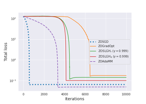
(a) CIFAR-10, Image ID = 56

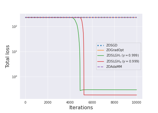
(b) CIFAR-10, Image ID = 34

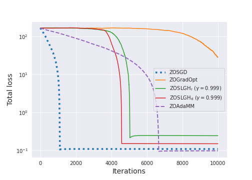
(c) CIFAR-10, Image ID = 102

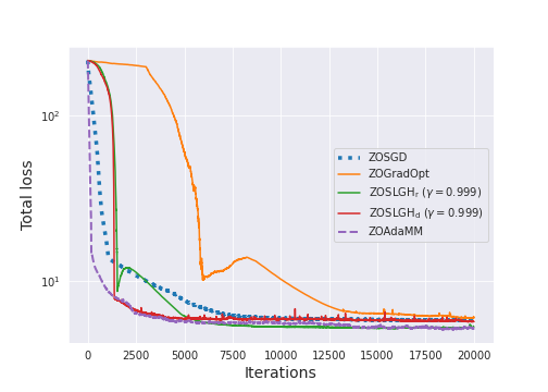
(d) MNIST, Image ID = 32

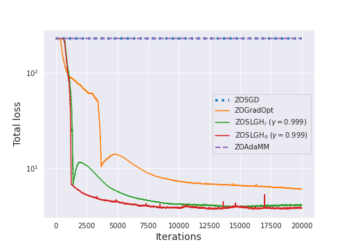
(e) MNIST, Image ID = 45

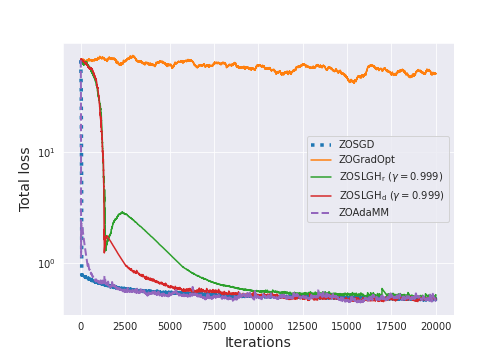
(f) MNIST, Image ID = 95

Figure 1:

Total loss for generating per-image black-box adversarial examples for different images

of CIFAR-10 and MNIST (log scale).

6 Summary and future work

We have presented here the deterministic/stochastic SLGH and ZOSLGH algorithms as well as their convergence results. They have been designed for the purpose of finding better solutions with fewer iterations by simplifying the homotopy process into a single loop. We consider this work to be a first attempt to improve the standard GH method.

Although this study has considered the case in which the accessible function contains some error and is possibly non-smooth, we assume the underlying objective function to be smooth. Further work should be carried out to investigate the case in which the objective function itself is non-smooth.

Acknowledgements

This work was supported by JSPS KAKENHI Grant Number 19H04069, JST ACT-I Grant Number JPMJPR18U5, and JST ERATO Grant Number JPMJER1903.

Appendix A Related work

Iteration complexity analysis for GH methods

To the best of our knowledge, there are no existing works that give theoretical guarantee for the convergence rate except for [Hazan et al. (2016)]. It characterized a parameterized family of non-convex functions referred to as “$\sigma$-nice”, for which a GH algorithm converges to a global optimum. Moreover, it derived the convergence rate to an $\epsilon$-optimal solution for the $\sigma$-nice function. The framework of $\sigma$-nice imposes the two conditions: (i) the solution obtained in each inner loop is located sufficiently close to an optimal solution of the optimization problem in the next inner loop; (ii) the optimization problem in each inner loop is strongly convex around its optimal solutions. Unfortunately, it is not obvious whether we can efficiently judge a function is “$\sigma$-nice”, and we cannot apply the analysis results to general non-convex functions. On the other hand, this work tackles a problem of different nature from [Hazan et al. (2016)] since it analyzes the convergence rate to an $\epsilon$-stationary point for general non-convex functions.

Guarantee for the value of the objective function

[Mobahi & Fisher III (2015b)] provided an upper bound on the objective value attained by a homotopy method. The bound was characterized by a quantity that they referred to as “optimization complexity”, which can be analytically computed when the objective function is expressed in some suitable basis functions such as Gaussian RBFs.

Other smoothing methods

Smoothing methods other than Gaussian smoothing include [Chen & Harker (1993); Chen (2012)]. The smoothing kernel in those works is simpler but restricted to specific problem settings. For example, [Chen (2012)] constructs smoothing approximations for optimization problems that can be reformulated by using the plus function $(t)_{+}:=\max\{0,t\}$.

Zeroth-order techniques

In problem settings in which the explicit gradient of the objective function cannot be calculated but the exact function values can be queried, zeroth-order optimization has become increasingly popular due to its potential for wide application. Such a class of applications appears in black-box adversarial attacks on deep neural networks [Chen et al. (2019)], structured prediction [Sokolov et al. (2016)], and reinforcement learning [Xu et al. (2020)]. Various zeroth-order methods (ZOSGD [Ghadimi & Lan (2013)], ZOAdaMM [Chen et al. (2019)], ZOSVRG [Liu et al. (2018)]) have been proposed for such black-box situations. All of them have been developed from ZOGD in [Nesterov & Spokoiny (2017)], which introduces random gradient-free oracles based on Gaussian smoothing with fixed $t$. This trend also applies to research on the GH method. [Hazan et al. (2016)] developed a GH method in the zeroth-order setting for which the objective is only accessible through a noisy value oracle. [Shao et al. (2019)] proposed a GH method for hyperparameter tuning based on [Hazan et al. (2016)] using two-point zeroth-order estimators [Nesterov & Spokoiny (2017)].

Appendix B Proofs for theorems and lemmas in Sections 3 and 4

Notation:

We sometimes denote the expectation with respect to random variables $\chi_{S+1},\ldots,\chi_{T}\ (S,T\in\mathbb{N},T>S)$ as $\mathbb{E}_{\chi}[\cdot]$ for the sake of simplicity.

B.1 Theorem 3.1

Proof for Theorem 3.1: Since the optimization problem (1) has an optimal value $f^{\ast}$ by Assumption A1 (ii), for any $t\in\mathcal{T}$ and for any $x\in\mathbb{R}^{d}$, we have

$$F(x,t)-f^{\ast}=\mathbb{E}_{u}[f(x+tu)-f^{\ast}]\geq 0.$$

Together with the relationship $F(x,0)=f(x)$, for any $x\in\mathbb{R}^{d}$, for any $t\in\mathcal{T}$ and for any optimal solution $x^{\ast}\in\mathbb{R}^{d}$ of the optimization problem (1), we have $F(x,t)-F(x^{\ast},0)\geq 0$. Furthermore, if we exclude cases where $f(x)$ is constant (a.e.), for any $(x,t)\in\mathbb{R}^{d}\times\mathcal{T}\setminus\{(x,0)\mid f(x)=f(x^{\ast})\}$, we obtain

$$F(x,t)-f^{\ast}=\mathbb{E}_{u}[f(x+tu)-f^{\ast}]>0.$$

Therefore, a minimum of the optimization problem of the GH function ${\mathop{\rm minimize}\limits_{x\in\mathbb{R}^{d},t\in\mathcal{T}}}\ F(x,t)$ holds only at $t=0$ and the corresponding $x$ becomes an optimal solution of the original optimization problem ${\mathop{\rm minimize}\limits_{x\in{\mathbb{R}}^{d}}}\ f(x)$. $\Box$

B.2 First-order SLGH algorithm

At the beginning of the subsection, we introduce a lemma that gives upper bounds for moments of Gaussian random variables, and then prove the two lemmas which appeared in the main paper.

Lemma B.1 (Lemma 1 in [Nesterov & Spokoiny (2017)]).

Let $u\in\mathbb{R}^{d}$ be a standard normal random variable. For $p\in[0,2]$, we have $\mathbb{E}_{u}[\|u\|^{p}]\leq d^{p/2}$. If $p\geq 2$, $\mathbb{E}_{u}[\|u\|^{p}]\leq(d+p)^{p/2}$ holds.

Proof for Lemma 3.2: According to the definition of Gaussian smoothing in the main paper, we have

$$|F(x,t)-F(y,t)| =\left|\int(f(x+tz)k(z)-f(y+tz)k(z))dz\right|$$

$$\leq\int\left|f(x+tz)-f(y+tz)\right|k(z)dz$$

$$\leq\int L_{0}\|x-y\|k(z)dz$$

$$\leq L_{0}\|x-y\|.$$

The proof of $L_{1}$-$smooth$ is similar to that of $L_{0}$-$Lipschitz$:

$$|\nabla_{x}F(x,t)-\nabla_{x}F(y,t)| \leq\int|\nabla f(x+tz)-\nabla f(y+tz)|k(z)dz$$

$$\leq\int L_{1}\|x-y\|k(z)dz$$

$$\leq L_{1}\|x-y\|.$$

$\Box$

The lemma has proved that the Lipschitz constants of $F(x,t)$ and $\nabla_{x}F(x,t)$ in terms of $x$ are smaller than those of $f(x)$ and $\nabla f(x)$, respectively. Therefore we can use the Lipschitz constants $L_{0}$ and $L_{1}$ of $f(x)$ and $\nabla f(x)$ for $F(x,t)$ and $\nabla_{x}F(x,t)$.

Proof for Lemma 3.3:

$$|F(x,t_{1})-F(x,t_{2})| =|\mathbb{E}_{u}[f(x+t_{1}u)-f(x+t_{2}u)]|$$

$$\leq\mathbb{E}_{u}[|f(x+t_{1}u)-f(x+t_{2}u)|]$$

$$\leq\mathbb{E}_{u}[L_{0}|t_{1}-t_{2}|\|u\|]$$

$$\leq L_{0}|t_{1}-t_{2}|\sqrt{d},$$

where the last inequality holds due to Lemma B.1. $\Box$

Before going to the convergence theorems, we introduce an additional useful lemma to estimate the gap between the gradient of the smoothed function and the true gradient.

Lemma B.2.

Let $f$ be a $L_{1}$-$smooth$ function.
(i) (Lemma 4 in [Nesterov & Spokoiny (2017)]) For any $x\in\mathbb{R}^{d}$ and $t>0$, we have

$$\|\nabla f(x)\|^{2}\leq 2\|\nabla_{x}F(x,t)\|^{2}+\frac{t^{2}}{2}L_{1}^{2}(d+6)^{3}.$$

(ii) Further, if $f$ is $L_{0}$-Lipschitz, for any $x\in\mathbb{R}^{d}$ and $t>0$, we have

$$\|\nabla f(x)\|^{2}\leq\|\nabla_{x}F(x,t)\|^{2}+tL_{0}L_{1}(d+3)^{3/2}.$$

Proof for (ii): We have

$$\|\nabla f(x)\|^{2}-\|\nabla_{x}F(x,t)\|^{2} =(\|\nabla f(x)\|+\|\nabla_{x}F(x,t)\|)(\|\nabla f(x)\|-\|\nabla_{x}F(x,t)\|)$$

$$\leq 2L_{0}(\|\nabla f(x)\|-\|\nabla_{x}F(x,t)\|)$$

$$\leq 2L_{0}\|\nabla_{x}F(x,t)-\nabla f(x)\|.$$

The term $\|\nabla_{x}F(x,t)-\nabla f(x)\|$ can be upper bounded as follows:

$$\|\nabla_{x}F(x,t)-\nabla f(x)\| \leq\left\|\mathbb{E}_{u}\left[\left(\frac{f(x+tu)-f(x)}{t}-\langle\nabla f(x),u\rangle\right)u\right]\right\|$$

$$\leq\mathbb{E}_{u}\left[\left|\frac{1}{t}\left(f(x+tu)-f(x)-t\langle\nabla f(x),u\rangle\right)\right|\|u\|\right]$$

$$\leq\mathbb{E}_{u}\left[\frac{tL_{1}}{2}\|u\|^{3}\right]$$

$$\leq\frac{tL_{1}}{2}(d+3)^{3/2},$$

where the last second inequality follows from a property of $L_{1}$-smooth function ($\forall x,y\in\mathbb{R}^{d},\ |f(y)-f(x)-\langle\nabla f(x),y-x\rangle|\leq\frac{L_{1}}{2}\|y-x\|^{2}$), and the last inequality holds due to Lemma B.1. Therefore, we obtain

$$\|\nabla f(x)\|^{2}\leq\|\nabla_{x}F(x,t)\|^{2}+tL_{0}L_{1}(d+3)^{3/2}.$$

Now, we are ready to prove Theorem 3.4.

Proof for Theorem 3.4: We follow the convergence analysis of gradient descent. According to Assumption A1 and Lemma 3.2, $F(x,t)$ is $L_{0}$-$Lipschitz$ and $L_{1}$-$smooth$ in terms of $x$. Therefore, we have

$$F(x_{k+1},t_{k}) \leq F(x_{k},t_{k})+\left<\nabla_{x}F(x_{k},t_{k}),(x_{k+1}-x_{k})\right>+\frac{L_{1}}{2}\|x_{k+1}-x_{k}\|^{2}$$

$$=F(x_{k},t_{k})-\left(\beta-\frac{L_{1}}{2}\beta^{2}\right)\|\nabla_{x}F(x_{k},t_{k})\|^{2},$$

where the last equation holds due to the updating rule of the gradient descent: $x_{k+1}-x_{k}=-\beta\nabla_{x}F(x_{k},t_{k})$. Then, we can get the upper bound for $\|\nabla_{x}F(x,t)\|^{2}$:

$$\left(\beta-\frac{L_{1}}{2}\beta^{2}\right)\|\nabla_{x}F(x_{k},t_{k})\|^{2} \leq F(x_{k},t_{k})-F(x_{k+1},t_{k})$$

$$=F(x_{k},t_{k})-F(x_{k+1},t_{k+1})+F(x_{k+1},t_{k+1})-F(x_{k+1},t_{k})$$

$$\leq F(x_{k},t_{k})-F(x_{k+1},t_{k+1})+L_{0}|t_{k+1}-t_{k}|\sqrt{d},$$

where the last inequality follows from Lemma 3.3.
Now, sum up the above inequality for all iterations $k_{0}+1\leq k\leq T\ (T>k_{0}\in\mathbb{N})$, and denote the minimum of $f$ as $f^{*}$, then we have

$$\left(\beta-\frac{L_{1}}{2}\beta^{2}\right)\sum_{k=k_{0}+1}^{T}\|\nabla_{x}F(x_{k},t_{k})\|^{2} \leq F(x_{k_{0}+1},t_{k_{0}+1})-F(x_{T+1},t_{T+1})+L_{0}\sqrt{d}\sum_{k=k_{0}+1}^{T}|t_{k+1}-t_{k}|$$

$$\leq F(x_{k_{0}+1},t_{k_{0}+1})-f^{*}+L_{0}\sqrt{d}\sum_{k={k_{0}+1}}^{T}|t_{k+1}-t_{k}|$$

$$\leq f(x_{k_{0}+1})-f^{*}+L_{0}\sqrt{d}\left(t_{k_{0}+1}+\sum_{k=k_{0}+1}^{T}|t_{k+1}-t_{k}|\right),$$ (10)

where the last inequality holds due to Lemma 3.3. Then, we can get the upper bound for $\|\nabla f(\hat{x})\|^{2}$ as

$$\|\nabla f(\hat{x})\|^{2}={\mathop{\rm min}\limits_{k\in[T]}}\|\nabla f(x_{k})\|^{2}$$

$$\leq{\mathop{\rm min}\limits_{k=k_{0}+1,\ldots,T}}\|\nabla f(x_{k})\|^{2}$$

$$\leq\frac{1}{T-k_{0}}\sum_{k=k_{0}+1}^{T}\|\nabla f(x_{k})\|^{2}$$

$$\leq\frac{1}{T-k_{0}}\sum_{k=k_{0}+1}^{T}\|\nabla_{x}F(x_{k},t_{k})\|^{2}+\frac{1}{T-k_{0}}L_{0}L_{1}(d+3)^{3/2}\sum_{k=k_{0}+1}^{T}t_{k}$$

$$\leq\frac{2\left(f(x_{k_{0}+1})-f^{*}+L_{0}\sqrt{d}\left(t_{k_{0}+1}+\sum_{k=k_{0}+1}^{T}|t_{k+1}-t_{k}|\right)\right)}{(T-k_{0})(2\beta-L_{1}\beta^{2})}+\frac{1}{T-k_{0}}L_{0}L_{1}(d+3)^{3/2}\sum_{k=k_{0}+1}^{T}t_{k},$$

where the third inequality holds due to Lemma B.2 (ii) and the last inequality follows from (10).

If we choose the step size $\beta$ as $\frac{1}{L_{1}}$, we have

$$\|\nabla f(\hat{x})\|^{2}$$

$$\leq\frac{2L_{1}\left(f(x_{k_{0}+1})-f^{*}+L_{0}\sqrt{d}\left(t_{k_{0}+1}+\sum_{k=k_{0}+1}^{T}|t_{k+1}-t_{k}|\right)\right)}{T-k_{0}}+\frac{1}{T-k_{0}}L_{0}L_{1}(d+3)^{3/2}\sum_{k=k_{0}+1}^{T}t_{k}$$

$$=O\left(\frac{1}{T-k_{0}}\left(1+d^{3/2}\sum_{k=k_{0}+1}^{T}t_{k}\right)\right),$$ (11)

where the last equality holds since $\sum_{k=k_{0}+1}^{T}|t_{k+1}-t_{k}|=O\left(\sum_{k=k_{0}+1}^{T}t_{k}\right)$ is satisfied. If we update $t_{k}$ as in Algorithm 2, we have $\sum_{k=k_{0}+1}^{T}t_{k}\leq\sum_{k=k_{0}+1}^{T}\max\{t_{1}\gamma^{k-1},\epsilon^{\prime}\}\leq\sum_{k=k_{0}+1}^{T}\left(t_{1}\gamma^{k-1}+\epsilon^{\prime}\right)\leq\frac{t_{1}\gamma^{k_{0}}}{1-\gamma}+\epsilon^{\prime}(T-k_{0}).$ By taking $\epsilon^{\prime}$ sufficiently close to $0$, together with the assumption of $1/(1-\gamma)=O(1)$, we have $\sum_{k=k_{0}+1}^{T}t_{k}=O(\gamma^{k_{0}})$. This implies that $\|\nabla f(\hat{x})\|^{2}\leq O(\frac{1+\gamma^{k_{0}}d^{3/2}}{T-k_{0}})$. Hence, we can obtain $\|\nabla f(\hat{x})\|\leq\epsilon$ in $T=k_{0}+O\left(\frac{1+\gamma^{k_{0}}d^{3/2}}{\epsilon^{2}}\right)$ iterations.

Now, set $k_{0}$ as $k_{0}=O\left(\frac{1}{\epsilon^{2}}\right)$, then, the iteration complexity can be bounded as $T=O\left(\frac{d^{3/2}}{\epsilon^{2}}\right)$. Furthermore, when $\gamma$ is chosen as $\gamma\leq d^{-3\epsilon^{2}/2}$, we can obtain $\gamma^{k_{0}}=O\left(d^{-3/2}\right)$ for some $k_{0}=O\left(\frac{1}{\epsilon^{2}}\right)$. This yields the iteration complexity of $T=O\left(\frac{1}{\epsilon^{2}}\right)$.

$\Box$

Before going to the proof of Theorem 3.5 in the stochastic setting, we prove that the gradient of the smoothed stochastic function $\nabla F(x,t;\xi)$ is unbiased, and it has a finite variance.

Lemma B.3.

Suppose that $f$ satisfies Assumption A1 (i) and Assumption A2.
(i) The stochastic gradient of the smoothed function $\nabla_{x}\bar{F}(x,t;\xi)$ becomes an unbiased estimator of $\nabla_{x}F(x,t)$. That is, for any $x\in\mathbb{R}^{d}$ and $t>0$, $\mathbb{E}_{\xi}[\nabla_{x}\bar{F}(x,t;\xi)]=\nabla_{x}F(x,t)$ holds.
(ii) For any $x\in\mathbb{R}^{d}$ and $t>0$, the variance of $\nabla_{x}\bar{F}(x,t;\xi)$ is bounded as $\mathbb{E}_{\xi}[\|\nabla_{x}\bar{F}(x,t;\xi)-\nabla_{x}F(x,t)\|^{2}]\leq\sigma^{2}$.

Proof for (i): From Assumption A1 (i), we can exchange the order of integration in terms of $\xi$ and $u$, which yields that

$$\mathbb{E}_{\xi}[\nabla_{x}\bar{F}(x,t;\xi)] =\mathbb{E}_{\xi}\left[\mathbb{E}_{u}\left[\frac{\bar{f}(x+tu;\xi)-\bar{f}(x;\xi)}{t}u\right]\right]$$

$$=\mathbb{E}_{u}\left[\mathbb{E}_{\xi}\left[\frac{\bar{f}(x+tu;\xi)-\bar{f}(x;\xi)}{t}u\right]\right]$$

$$=\mathbb{E}_{u}\left[\frac{f(x+tu)-f(x)}{t}u\right]$$

$$=\nabla_{x}F(x,t).$$

Proof for (ii): We have

$$\mathbb{E}_{\xi}[\|\nabla_{x}\bar{F}(x,t;\xi)-\nabla_{x}F(x,t)\|^{2}] =\mathbb{E}_{\xi}[\|\nabla_{x}\mathbb{E}_{u}[\bar{f}(x+tu;\xi)]-\nabla_{x}\mathbb{E}_{u}[f(x+tu)]\|^{2}]$$

$$=\mathbb{E}_{\xi}[\|\mathbb{E}_{u}[\nabla_{x}\bar{f}(x+tu;\xi)-\nabla f(x+tu)]\|^{2}]$$

$$\leq\mathbb{E}_{\xi}[\mathbb{E}_{u}[\|\nabla_{x}\bar{f}(x+tu;\xi)-\nabla f(x+tu)\|^{2}]]$$

$$=\mathbb{E}_{u}[\mathbb{E}_{\xi}[\|\nabla_{x}\bar{f}(x+tu;\xi)-\nabla f(x+tu)\|^{2}]]$$

$$\leq\sigma^{2},$$

where the second and third equalities hold due to Assumption A1 (i), and the last inequality follows from Assumption A2 (ii).

Proof for Theorem 3.5: Denote $\delta_{k}:=\nabla_{x}\bar{F}(x_{k},t_{k};\xi_{k})-\nabla_{x}F(x_{k},t_{k})$. We follow the convergence analysis of stochastic gradient descent. According to Lemma 3.2, since $f(x)$ is $L_{0}$-$Lipschitz$ and $L_{1}$-$smooth$, $F(x,t)$ is also $L_{0}$-$Lipschitz$ and $L_{1}$-$smooth$ in terms of $x$. Thus, we have

$$F(x_{k+1},t_{k}) \leq F(x_{k},t_{k})+\left<\nabla_{x}F(x_{k},t_{k}),(x_{k+1}-x_{k})\right>+\frac{L_{1}}{2}\|x_{k+1}-x_{k}\|^{2}$$

$$=F(x_{k},t_{k})-\beta\left<\nabla_{x}F(x_{k},t_{k}),\nabla_{x}\bar{F}(x_{k},t_{k};\xi_{k})\right>+\frac{L_{1}}{2}\beta^{2}\|\nabla_{x}\bar{F}(x_{k},t_{k};\xi_{k})\|^{2}$$

$$=F(x_{k},t_{k})-\left(\beta-\frac{L_{1}}{2}\beta^{2}\right)\|\nabla_{x}F(x_{k},t_{k})\|^{2}-(\beta-L_{1}\beta^{2})\left<\nabla_{x}F(x_{k},t_{k}),\delta_{k}\right>+\frac{L_{1}}{2}\beta^{2}\|\delta_{k}\|^{2},$$ (12)

where the first equation holds due to the updating rule $x_{k+1}-x_{k}=-\beta\nabla_{x}\bar{F}(x_{k},t_{k};\xi_{k})$, and the last equation holds due to the definition of $\delta_{k}$. Denote

$$A_{k}:=-(\beta-L_{1}\beta^{2})\left<\nabla_{x}F(x_{k},t_{k}),\delta_{k}\right>+\frac{L_{1}}{2}\beta^{2}\|\delta_{k}\|^{2}$$

for simplicity. From (12), we obtain the upper bound for $\|\nabla_{x}F(x,t)\|^{2}$ as follows:

$$\left(\beta-\frac{L_{1}}{2}\beta^{2}\right)\|\nabla_{x}F(x_{k},t_{k})\|^{2} \leq F(x_{k},t_{k})-F(x_{k+1},t_{k})+A_{k}$$

$$=F(x_{k},t_{k})-F(x_{k+1},t_{k+1})+F(x_{k+1},t_{k+1})-F(x_{k+1},t_{k})+A_{k}$$

$$\leq F(x_{k},t_{k})-F(x_{k+1},t_{k+1})+L_{0}|t_{k+1}-t_{k}|\sqrt{d}+A_{k},$$

where the last inequality follows from Lemma 3.3.
Now, sum up the above inequality for all iterations $k_{0}+1\leq k\leq T\ (k_{0}<T)$. Then we have

$$\left(\beta-\frac{L_{1}}{2}\beta^{2}\right)\sum_{k=k_{0}+1}^{T}\|\nabla_{x}F(x_{k},t_{k})\|^{2}$$

$$\leq F(x_{k_{0}+1},t_{k_{0}+1})-F(x_{T+1},t_{T+1})+L_{0}\sqrt{d}\sum_{k=k_{0}+1}^{T}|t_{k+1}-t_{k}|+\sum_{k=k_{0}+1}^{T}A_{k}$$

$$\leq F(x_{k_{0}+1},t_{k_{0}+1})-f^{*}+L_{0}\sqrt{d}\sum_{k=k_{0}+1}^{T}|t_{k+1}-t_{k}|+\sum_{k=k_{0}+1}^{T}A_{k}.$$

$$\leq f(x_{k_{0}+1})-f^{*}+L_{0}\sqrt{d}\left(t_{k_{0}+1}+\sum_{k=k_{0}+1}^{T}|t_{k+1}-t_{k}|\right)+\sum_{k=k_{0}+1}^{T}A_{k}.$$

Take the expectation with respect to the random vectors $\{\xi_{k_{0}+1},\ldots,\xi_{T}\}$, then we have

$$\left(\beta-\frac{L_{1}}{2}\beta^{2}\right)\sum_{k=k_{0}+1}^{T}\mathbb{E}_{\xi}[\|\nabla_{x}F(x_{k},t_{k})\|^{2}]$$

$$\leq f(x_{k_{0}+1})-f^{*}+L_{0}\sqrt{d}\left(t_{k_{0}+1}+\sum_{k=k_{0}+1}^{T}\mathbb{E}_{\xi}[|t_{k+1}-t_{k}|]\right)+\sum_{k=k_{0}+1}^{T}\mathbb{E}_{\xi}[A_{k}].$$ (13)

The expectation of $A_{k}$ is evaluated as

$$\sum_{k=k_{0}+1}^{T}\mathbb{E}_{\xi}[A_{k}] =-\sum_{k=k_{0}+1}^{T}(\beta-L_{1}\beta^{2})\mathbb{E}_{\xi}[\left<\nabla_{x}F(x_{k},t_{k}),\delta_{k}\right>]+\sum_{k=k_{0}+1}^{T}\frac{L_{1}}{2}\beta^{2}\mathbb{E}_{\xi}[\|\delta_{k}\|^{2}]$$

$$\leq(T-k_{0})\frac{L_{1}}{2}\beta^{2}\sigma^{2},$$ (14)

where the last equality holds due to Lemma B.3 (ii) ($\mathbb{E}_{\xi}[\|\delta_{k}\|^{2}]\leq\sigma^{2}$) and the fact that each point $x_{k}$ is a function of the history $\xi_{[k-1]}$ in the random process, thus $\mathbb{E}_{\xi_{k}}[\left<\nabla_{x}F(x_{k},t_{k}),\delta_{k}\right>\mid\xi_{[k-1]}]=0$.

Then, we can estimate the upper bound for $\mathbb{E}_{\xi,k^{\prime}}[\|\nabla f(\hat{x})\|^{2}]$ as

$$\mathbb{E}_{\xi,k^{\prime}}[\|\nabla f(\hat{x})\|^{2}]=\frac{1}{T-k_{0}}\sum_{k=k_{0}+1}^{T}\mathbb{E}_{\xi}[\|\nabla f(x_{k})\|^{2}]$$

$$\leq\frac{1}{T-k_{0}}\sum_{k=k_{0}+1}^{T}\mathbb{E}_{\xi}[\|\nabla_{x}F(x_{k},t_{k})\|^{2}]+\frac{1}{T-k_{0}}L_{0}L_{1}(d+3)^{3/2}\sum_{k=k_{0}+1}^{T}\mathbb{E}_{\xi}[t_{k}]$$

$$\leq\frac{2\left(f(x_{k_{0}+1})-f^{*}+L_{0}\sqrt{d}\left(t_{k_{0}+1}+\sum_{k=k_{0}+1}^{T}\mathbb{E}_{\xi}[|t_{k+1}-t_{k}|]\right)\right)}{(T-k_{0})(2\beta-L_{1}\beta^{2})}$$

$$+\frac{1}{T-k_{0}}L_{0}L_{1}(d+3)^{3/2}\sum_{k=k_{0}+1}^{T}\mathbb{E}_{\xi}[t_{k}]+\frac{L_{1}\beta^{2}\sigma^{2}}{2\beta-L_{1}\beta^{2}},$$

where the first inequality holds due to Lemma B.2 (ii) and the last inequality follows from (13) and (14).

If the step size $\beta$ is chosen as $\beta=\mathop{\rm min}\ \{\frac{1}{L_{1}},\frac{1}{\sqrt{T-k_{0}}}\}$, then we have

$$\frac{1}{2\beta-L_{1}\beta^{2}}\leq\frac{1}{\beta},$$

$$\frac{1}{\beta}\leq L_{1}+\sqrt{T-k_{0}}.$$

Hence, we can obtain

$$\frac{2\left(f(x_{k_{0}+1})-f^{*}+L_{0}\sqrt{d}\left(t_{k_{0}+1}+\sum_{k=k_{0}+1}^{T}\mathbb{E}_{\xi}[|t_{k+1}-t_{k}|]\right)\right)}{(T-k_{0})(2\beta-L_{1}\beta^{2})}$$

$$+\frac{1}{T-k_{0}}L_{0}L_{1}(d+3)^{3/2}\sum_{k=k_{0}+1}^{T}\mathbb{E}_{\xi}[t_{k}]+\frac{L_{1}\beta^{2}\sigma^{2}}{2\beta-L_{1}\beta^{2}}$$

$$=O\left(\frac{1+\sqrt{d}\mathbb{E}_{\xi}\left[\sum_{k=k_{0}+1}^{T}|t_{k+1}-t_{k}|\right]}{\sqrt{T-k_{0}}}+\frac{d^{3/2}}{T-k_{0}}\mathbb{E}_{\xi}\left[\sum_{k=k_{0}+1}^{T}t_{k}\right]\right).$$

If $t_{k}$ is updated as in Algorithm 2, we have $\sum_{k=k_{0}+1}^{T}|t_{k+1}-t_{k}|\leq t_{1}\gamma_{k_{0}}=O(\gamma^{k_{0}})$ and $\sum_{k=k_{0}+1}^{T}t_{k}\leq\frac{t_{1}\gamma^{k_{0}}}{1-\gamma}+\epsilon^{\prime}T=O(\gamma^{k_{0}})$ in the same argument that showed Theorem 3.4. Combining the above inequalities, we obtain

$$\mathbb{E}_{\xi,k^{\prime}}[\|\nabla f(\hat{x})\|^{2}]=\frac{1}{T-k_{0}}\sum_{k=k_{0}+1}^{T}\mathbb{E}_{\xi}[\|\nabla f(x_{k})\|^{2}]=O\left(\frac{1+\sqrt{d}\gamma^{k_{0}}}{\sqrt{T-k_{0}}}+\frac{d^{3/2}\gamma^{k_{0}}}{T-k_{0}}\right).$$ (15)

Here, we have $k_{0}=O\left(\frac{1}{\epsilon^{4}}\right)$ by the definition of $k_{0}$. Thus, by setting $T=k_{0}+O\left(\frac{d}{\epsilon^{4}}+\frac{d^{3/2}}{\epsilon^{2}}\right)=O\left(\frac{d}{\epsilon^{4}}+\frac{d^{3/2}}{\epsilon^{2}}\right)$, we can obtain $\mathbb{E}_{\xi,k^{\prime}}[\|\nabla f(\hat{x})\|^{2}]\leq\epsilon^{2}$. This implies $\mathbb{E}_{\xi,k^{\prime}}[\|\nabla f(\hat{x})\|]\leq\epsilon$ as $\mathbb{E}_{\xi,k^{\prime}}[\|\nabla f(\hat{x})\|]^{2}\leq\mathbb{E}_{\xi,k^{\prime}}[\|\nabla f(\hat{x})\|^{2}]$ follows from Jensen’s inequality. Furthermore, when $\gamma$ is chosen as $\gamma\leq(\max\{d^{1/2},d^{3/2}\epsilon^{2}\})^{-\epsilon^{4}}$ , we have $\log_{\gamma}\min\{d^{-1/2},d^{-3/2}\epsilon^{-2}\}=O\left(\frac{1}{\epsilon^{4}}\right)$, which implies $k_{0}=\Omega(\log_{\gamma}\min\{d^{-1/2},d^{-3/2}\epsilon^{-2}\}).$ Therefore, we can obtain $\gamma^{k_{0}}=O\left(\min\{d^{-1/2},d^{-3/2}\epsilon^{-2}\})\right)$ , which yields the iteration complexity of $T=O\left(\frac{1}{\epsilon^{4}}\right)$.

$\Box$

B.3 Zeroth-order SLGH algorithm

In the zeroth-order setting, we can evaluate the gap between the zeroth-order gradient estimator and the true gradient using the following lemma.

Lemma B.4 (Theorem 4 in [Nesterov & Spokoiny (2017)]).

Let $f$ be a $L_{1}$-$smooth$ function, then for any $x\in\mathbb{R}^{d}$ and for any $t>0$, we have

$$\mathbb{E}_{u}\left[\frac{1}{t^{2}}(f(x+tu)-f(x))^{2}\|u\|^{2}\right]\leq\frac{t^{2}}{2}L_{1}^{2}(d+6)^{3}+2(d+4)\|\nabla f(x)\|^{2}.$$

Proof for Theorem 4.1: Let $w_{k}:=(u_{k},v_{k}),\ k\in[T]$, and denote $\delta_{k}:=\tilde{g}_{x}(x_{k},t_{k};u_{k})-\nabla_{x}F(x_{k},t_{k})$, where $\tilde{g}_{x}(x_{k},t_{k};u_{k})$ is the zeroth-order estimator of gradient defined in the main paper. Utilize the updating rule of $x$ and $L_{1}$-smoothness of $F(x,t)$ in terms of $x$. Then we have

$$F(x_{k+1},t_{k}) \leq F(x_{k},t_{k})+\left<\nabla_{x}F(x_{k},t_{k}),(x_{k+1}-x_{k})\right>+\frac{L_{1}}{2}\|x_{k+1}-x_{k}\|^{2}$$

$$=F(x_{k},t_{k})-\beta\left<\nabla_{x}F(x_{k},t_{k}),\tilde{g}_{x}(x_{k},t_{k};u_{k})\right>+\frac{L_{1}}{2}\beta^{2}\|\tilde{g}_{x}(x_{k},t_{k};u_{k})\|^{2}$$

$$=F(x_{k},t_{k})-\beta\|\nabla_{x}F(x_{k},t_{k})\|^{2}-\beta\left<\nabla_{x}F(x_{k},t_{k}),\delta_{k}\right>+\frac{L_{1}}{2}\beta^{2}\|\tilde{g}_{x}(x_{k},t_{k};u_{k}))\|^{2},$$ (16)

where the first equation holds due to the updating rule $x_{k+1}-x_{k}=-\beta\tilde{g}_{x}(x_{k},t_{k};u_{k})$.
Denote

$$B_{k}:=-\beta\left<\nabla_{x}F(x_{k},t_{k}),\delta_{k}\right>+\frac{L_{1}}{2}\beta^{2}\|\tilde{g}_{x}(x_{k},t_{k};u_{k})\|^{2}$$

for simplicity. From Lemma 3.3 and (16), we get the upper bound for $\|\nabla_{x}F(x,t)\|^{2}$ as

$$\beta\|\nabla_{x}F(x_{k},t_{k})\|^{2} \leq F(x_{k},t_{k})-F(x_{k+1},t_{k})+B_{k}$$

$$=F(x_{k},t_{k})-F(x_{k+1},t_{k+1})+F(x_{k+1},t_{k+1})-F(x_{k+1},t_{k})+B_{k}$$

$$\leq F(x_{k},t_{k})-F(x_{k+1},t_{k+1})+L_{0}|t_{k+1}-t_{k}|\sqrt{d}+B_{k}.$$

Now, sum up the above inequality for all iterations $k_{0}+1\leq k\leq T\ (k_{0}<T)$. Then we have

$$\sum_{k=k_{0}+1}^{T}\beta\|\nabla_{x}F(x_{k},t_{k})\|^{2} \leq F(x_{k_{0}+1},t_{k_{0}+1})-F(x_{T+1},t_{T+1})+L_{0}\sum_{k=k_{0}+1}^{T}|t_{k+1}-t_{k}|\sqrt{d}+\sum_{k=k_{0}+1}^{T}B_{k}$$

$$\leq F(x_{k_{0}+1},t_{k_{0}+1})-f^{*}+L_{0}\sqrt{d}\sum_{k=k_{0}+1}^{T}|t_{k+1}-t_{k}|+\sum_{k=k_{0}+1}^{T}B_{k}$$

$$\leq f(x_{k_{0}+1})-f^{*}+L_{0}\sqrt{d}\left(t_{k_{0}+1}+\sum_{k=k_{0}+1}^{T}|t_{k+1}-t_{k}|\right)+\sum_{k=k_{0}+1}^{T}B_{k}.$$

Next, take the expectations with respect to random vectors $\{w_{k_{0}+1},\ldots,w_{T}\}$ on both sides. Then we can get

$$\sum_{k=k_{0}+1}^{T}\beta\mathbb{E}_{w}[\|\nabla_{x}F(x_{k},t_{k})\|^{2}] \leq f(x_{k_{0}+1})-f^{*}+L_{0}\sqrt{d}\left(t_{k_{0}+1}+\sum_{k=k_{0}+1}^{T}\mathbb{E}_{w}[|t_{k+1}-t_{k}|]\right)$$

$$+\sum_{k=k_{0}+1}^{T}\mathbb{E}_{w}[B_{k}].$$ (17)

Observe by the definition of $\tilde{g}_{x}(x_{k},t_{k};u_{k})$ in the main paper that $\mathbb{E}_{u_{k}}[\tilde{g}_{x}(x_{k},t_{k};u_{k})\mid u_{[k-1]}]=\nabla_{x}F(x_{k},t_{k})$, thus $\mathbb{E}_{w_{k}}[\left<\nabla_{x}F(x_{k},t_{k}),\delta_{k}\right>\mid w_{[k-1]}]=0$ holds. Then we have

$$\mathbb{E}_{w_{k}}[B_{k}\mid w_{[k-1]}] =-\beta\mathbb{E}_{w_{k}}[\left<\nabla_{x}F(x_{k},t_{k}),\delta_{k}\right>\mid w_{[k-1]}]+\frac{L_{1}}{2}\beta^{2}\mathbb{E}_{w_{k}}[\|\tilde{g}_{x}(x_{k},t_{k};u_{k})\|^{2}\mid w_{[k-1]}]$$

$$\leq\frac{L_{1}}{2}\beta^{2}\left(\frac{\mathbb{E}_{w_{k}}[t_{k}^{2}\mid w_{[k-1]}]}{2}L_{1}^{2}(d+6)^{3}+2(d+4)\mathbb{E}_{w_{k}}[\|\nabla f(x_{k})\|^{2}\mid w_{[k-1]}]\right)$$

$$=\frac{\mathbb{E}_{w_{k}}[t_{k}^{2}\mid w_{[k-1]}]}{4}L_{1}^{3}\beta^{2}(d+6)^{3}+L_{1}\beta^{2}(d+4)\mathbb{E}_{w_{k}}[\|\nabla f(x_{k})\|^{2}\mid w_{[k-1]}],$$ (18)

where the inequality holds due to Lemma B.4.

Lemma B.2 (ii) together with the above inequalities yields that

$$\sum_{k=k_{0}+1}^{T}\beta\mathbb{E}_{w}[\|\nabla f(x_{k})\|^{2}]$$

$$\leq\sum_{k=k_{0}+1}^{T}\beta\mathbb{E}_{w}[\|\nabla_{x}F(x_{k},t_{k})\|^{2}]+\sum_{k=k_{0}+1}^{T}\beta L_{0}L_{1}(d+3)^{3/2}\mathbb{E}_{w}[t_{k}]$$

$$\leq f(x_{k_{0}+1})-f^{*}+L_{0}\sqrt{d}\left(t_{k_{0}+1}+\sum_{k=k_{0}+1}^{T}\mathbb{E}_{w}[|t_{k+1}-t_{k}|]\right)+\sum_{k=k_{0}+1}^{T}\mathbb{E}_{w}[B_{k}]$$

$$+\sum_{k=k_{0}+1}^{T}\beta L_{0}L_{1}(d+3)^{3/2}\mathbb{E}_{w}[t_{k}]$$

$$\leq f(x_{k_{0}+1})-f^{*}+L_{0}\sqrt{d}\left(t_{k_{0}+1}+\sum_{k=k_{0}+1}^{T}\mathbb{E}_{w}[|t_{k+1}-t_{k}|]\right)+\sum_{k=k_{0}+1}^{T}\frac{\mathbb{E}_{w}[t_{k}^{2}]}{4}L_{1}^{3}\beta^{2}(d+6)^{3}$$

$$+\sum_{k=k_{0}+1}^{T}L_{1}\beta^{2}(d+4)\mathbb{E}_{w}[\|\nabla f(x_{k})\|^{2}]+\sum_{k=k_{0}+1}^{T}\beta L_{0}L_{1}(d+3)^{3/2}\mathbb{E}_{w}[t_{k}],$$ (19)

where the second inequality holds due to (17), and the last inequality follows from (B.3). Rearrange the terms in the above inequality. Then we can get

$$(\beta-(d+4)L_{1}\beta^{2})\sum_{k=k_{0}+1}^{T}\mathbb{E}_{w}[\|\nabla f(x_{k})\|^{2}] \leq f(x_{k_{0}+1})-f^{*}+L_{0}\sqrt{d}\left(t_{k_{0}+1}+\sum_{k=k_{0}+1}^{T}\mathbb{E}_{w}[|t_{k+1}-t_{k}|]\right)$$

$$+\frac{L_{1}^{3}\beta^{2}(d+6)^{3}}{4}\sum_{k=k_{0}+1}^{T}\mathbb{E}_{w}[t_{k}^{2}]+L_{0}L_{1}\beta(d+3)^{3/2}\sum_{k=k_{0}+1}^{T}\mathbb{E}_{w}[t_{k}].$$ (20)

Divide both sides of the above inequality by $(T-k_{0})(\beta-(d+4)L_{1}\beta^{2})$ and set the step size $\beta$ as $\frac{1}{2(d+4)L_{1}}$. Since $\frac{1}{\beta-(d+4)L_{1}\beta^{2}}\leq 4(d+4)L_{1}$ holds, we can obtain

$$\frac{1}{T-k_{0}}\sum_{k=k_{0}+1}^{T}\mathbb{E}_{w}[\|\nabla f(x_{k})\|^{2}] \leq\frac{4(d+4)L_{1}}{T-k_{0}}\left(f(x_{k_{0}+1})-f^{*}+L_{0}\sqrt{d}\left(t_{k_{0}+1}+\sum_{k=k_{0}+1}^{T}\mathbb{E}_{w}[|t_{k+1}-t_{k}|]\right)\right.$$

$$\left.+\frac{L_{1}(d+6)^{3}}{16(d+4)^{2}}\sum_{k=k_{0}+1}^{T}\mathbb{E}_{w}[t_{k}^{2}]+\frac{L_{0}(d+3)^{3/2}}{2(d+4)}\sum_{k=k_{0}+1}^{T}\mathbb{E}_{w}[t_{k}]\right)$$

$$=O\left(\frac{d}{T-k_{0}}\left(1+d\mathbb{E}_{w}\left[\sum_{k=k_{0}+1}^{T}t_{k}^{2}\right]+\sqrt{d}\mathbb{E}_{w}\left[\sum_{k=k_{0}+1}^{T}t_{k}\right]\right)\right)$$

$$=O\left(\frac{d}{T-k_{0}}\left(1+d\gamma^{2k_{0}}+\sqrt{d}\gamma^{k_{0}}\right)\right),$$ (21)

where the last equality follows from the update rule of $t_{k}$, as shown in the proof of Theorem 3.4 as well.

Here, we have $k_{0}=O\left(\frac{d}{\epsilon^{2}}\right)$ by the definition of $k_{0}$. Thus, by setting $T=k_{0}+O\left(\frac{d^{2}}{\epsilon^{2}}\right)=O\left(\frac{d^{2}}{\epsilon^{2}}\right)$, we can obtain $\mathbb{E}_{w,k^{\prime}}[\|\nabla f(\hat{x})\|^{2}]=\frac{1}{T-k_{0}}\sum_{k=k_{0}+1}^{T}\mathbb{E}_{w}[\|\nabla f(x_{k})\|^{2}]\leq\epsilon^{2}$. This implies $\mathbb{E}_{w,k^{\prime}}[\|\nabla f(\hat{x})\|]\leq\epsilon$ as $\mathbb{E}_{w,k^{\prime}}[\|\nabla f(\hat{x})\|]^{2}\leq\mathbb{E}_{w,k^{\prime}}[\|\nabla f(\hat{x})\|^{2}]$ follows from Jensen’s inequality. Furthermore, when $\gamma$ is chosen as $\gamma\leq d^{-\epsilon^{2}/2d}$ , we have $\log_{\gamma}d^{-1/2}=O\left(\frac{d}{\epsilon^{2}}\right)$, which implies $k_{0}=\Omega\left(\log_{\gamma}d^{-1/2}\right)$. Therefore, we can obtain $\gamma^{k_{0}}=O(d^{-1/2})$, which yields the iteration complexity of $T=O\left(\frac{d}{\epsilon^{2}}\right)$.

$\Box$

Proof for Theorem 4.2: Let $\zeta_{k}:=(\xi_{k},u_{k},v_{k})$, $k\in[T]$ and denote $\delta_{k}:=\tilde{G}_{x}(x_{k},t_{k};\xi_{k},u_{k})-\nabla_{x}F(x_{k},t_{k})$. As discussed in the main paper, we have

$$\mathbb{E}_{\xi,u}[\tilde{G}_{x}(x,t;\xi,u)]=\mathbb{E}_{u}[\mathbb{E}_{\xi}[\tilde{G}_{x}(x,t;\xi,u)|u]]=\nabla_{x}F(x,t).$$ (22)

From the update rule for $x$, we can obtain

$$F(x_{k+1},t_{k}) \leq F(x_{k},t_{k})+\left<\nabla_{x}F(x_{k},t_{k}),(x_{k+1}-x_{k})\right>+\frac{L_{1}}{2}\|x_{k+1}-x_{k}\|^{2}$$

$$=F(x_{k},t_{k})-\beta\left<\nabla_{x}F(x_{k},t_{k}),\tilde{G}_{x}(x_{k},t_{k};\xi_{k},u_{k})\right>+\frac{L_{1}}{2}\beta^{2}\|\tilde{G}_{x}(x_{k},t_{k};\xi_{k},u_{k})\|^{2}$$

$$=F(x_{k},t_{k})-\beta\|\nabla_{x}F(x_{k},t_{k})\|^{2}-\beta\left<\nabla_{x}F(x_{k},t_{k}),\delta_{k}\right>+\frac{L_{1}}{2}\beta^{2}\|\tilde{G}_{x}(x_{k},t_{k};\xi_{k},u_{k})\|^{2}.$$

Now, denote

$$D_{k}:=-\beta\left<\nabla_{x}F(x_{k},t_{k}),\delta_{k}\right>+\frac{L_{1}}{2}\beta^{2}\|\tilde{G}_{x}(x_{k},t_{k};\xi_{k},u_{k})\|^{2}$$

for simplicity. Then, we can get the upper bound for $\|\nabla_{x}F(x,t)\|^{2}$ with $D_{k}$:

$$\beta\|\nabla_{x}F(x_{k},t_{k})\|^{2} \leq F(x_{k},t_{k})-F(x_{k+1},t_{k})+D_{k}$$

$$=F(x_{k},t_{k})-F(x_{k+1},t_{k+1})+F(x_{k+1},t_{k+1})-F(x_{k+1},t_{k})+D_{k}$$

$$\leq F(x_{k},t_{k})-F(x_{k+1},t_{k+1})+L_{0}|t_{k+1}-t_{k}|\sqrt{d}+D_{k}.$$

Sum up the above inequality for all iterations $k_{0}+1\leq k\leq T\ (T>k_{0})$. Then we have

$$\sum_{k=k_{0}+1}^{T}\beta\|\nabla_{x}F(x_{k},t_{k})\|^{2}$$

$$\leq F(x_{k_{0}+1},t_{k_{0}+1})-F(x_{T+1},t_{T+1})+L_{0}\sqrt{d}\sum_{k=k_{0}+1}^{T}|t_{k+1}-t_{k}|+\sum_{k=k_{0}+1}^{T}D_{k}$$

$$\leq F(x_{k_{0}+1},t_{k_{0}+1})-f^{*}+L_{0}\sqrt{d}\sum_{k=k_{0}+1}^{T}|t_{k+1}-t_{k}|+\sum_{k=k_{0}+1}^{T}D_{k}$$

$$\leq f(x_{k_{0}+1})-f^{*}+L_{0}\sqrt{d}\left(t_{k_{0}+1}+\sum_{k=k_{0}+1}^{T}|t_{k+1}-t_{k}|\right)+\sum_{k=k_{0}+1}^{T}D_{k},$$ (23)

where the last inequality follows from Lemma 3.3. Observe from (22) that

$$\mathbb{E}_{\zeta_{k}}[\left<\nabla_{x}F(x_{k},t_{k}),\delta_{k}\right>\mid\zeta_{[k-1]}]=0.$$

Thus, we have

$$\mathbb{E}_{\zeta_{k}}[D_{k}\mid\zeta_{[k-1]}] =-\beta\mathbb{E}_{\zeta_{k}}[\left<\nabla_{x}F(x_{k},t_{k}),\delta_{k}\right>\mid\zeta_{[k-1]}]+\frac{L_{1}}{2}\beta^{2}\mathbb{E}_{\zeta_{k}}[\|\tilde{G}_{x}(x_{k},t_{k};\xi_{k},u_{k})\|^{2}\mid\zeta_{[k-1]}]$$

$$=\frac{L_{1}}{2}\beta^{2}\mathbb{E}_{\zeta_{k}}(\|\tilde{G}_{x}(x_{k},t_{k};\xi_{k},u_{k})\|^{2}\mid\zeta_{[k-1]})$$

$$\leq\frac{L_{1}}{2}\beta^{2}\left(\frac{\mathbb{E}_{\zeta_{k}}[t_{k}^{2}\mid\zeta_{[k-1]}]}{2}L_{1}^{2}(d+6)^{3}+2(d+4)(\mathbb{E}_{\zeta_{k}}[\|\nabla_{x}\bar{f}(x_{k};\xi_{k})\mid\zeta_{[k-1]}\|^{2}])\right)$$

$$\leq\frac{L_{1}}{2}\beta^{2}\left(\frac{\mathbb{E}_{\zeta_{k}}[t_{k}^{2}\mid\zeta_{[k-1]}]}{2}L_{1}^{2}(d+6)^{3}+2(d+4)(\mathbb{E}_{\zeta_{k}}[\|\nabla f(x_{k})\mid\zeta_{[k-1]}\|^{2}]+\sigma^{2})\right),$$ (24)

where the fist inequality follows from Lemma B.4 and the last inequality holds due to Assumption A2 (ii).

Take the expectation for (23) with respect to $\zeta_{k_{0}+1},\ldots,\zeta_{T}$. Together with Lemma B.2 (ii), we have

$$\sum_{k=k_{0}+1}^{T}\beta\mathbb{E}_{\zeta}[\|\nabla f(x_{k})\|^{2}]$$

$$\leq\sum_{k=k_{0}+1}^{T}\beta\mathbb{E}_{\zeta}[\|\nabla_{x}F(x_{k},t_{k})\|^{2}]+\sum_{k=k_{0}+1}^{T}\beta\mathbb{E}_{\zeta}[t_{k}]L_{0}L_{1}(d+3)^{3/2}$$

$$\leq f(x_{k_{0}+1})-f^{*}+L_{0}\sqrt{d}\left(t_{k_{0}+1}+\sum_{k=k_{0}+1}^{T}\mathbb{E}_{\zeta}[|t_{k+1}-t_{k}|]\right)+\sum_{k=k_{0}+1}^{T}\mathbb{E}_{\zeta}[D_{k}]$$

$$+\sum_{k=k_{0}+1}^{T}\mathbb{E}_{\zeta}[t_{k}]L_{0}L_{1}\beta(d+3)^{3/2}$$

$$\leq f(x_{k_{0}+1})-f^{*}+L_{0}\sqrt{d}\left(t_{k_{0}+1}+\sum_{k=k_{0}+1}^{T}\mathbb{E}_{\zeta}[|t_{k+1}-t_{k}|]\right)+\sum_{k=k_{0}+1}^{T}\mathbb{E}_{\zeta}[t_{k}]L_{0}L_{1}\beta(d+3)^{3/2}$$

$$+\sum_{k=k_{0}+1}^{T}\frac{\mathbb{E}_{\zeta}[t_{k}^{2}]}{4}L_{1}^{3}\beta^{2}(d+6)^{3}+\sum_{k=k_{0}+1}^{T}L_{1}\beta^{2}(d+4)\mathbb{E}_{\zeta}[\|\nabla f(x_{k})\|^{2}]+L_{1}\beta^{2}(d+4)\sigma^{2}(T-k_{0}),$$

where the last inequality holds due to (24). Rearrange the terms in the above inequality. Then we can get

$$(\beta-(d+4)L_{1}\beta^{2})\sum_{k=k_{0}+1}^{T}\mathbb{E}_{\zeta}[\|\nabla f(x_{k})\|^{2}] \leq f(x_{k_{0}+1})-f^{*}+L_{0}\sqrt{d}\left(t_{k_{0}+1}+\sum_{k=k_{0}+1}^{T}\mathbb{E}_{\zeta}[|t_{k+1}-t_{k}|]\right)$$

$$+\frac{L_{1}^{3}\beta^{2}(d+6)^{3}}{4}\sum_{k=k_{0}+1}^{T}\mathbb{E}_{\zeta}[t_{k}^{2}]+L_{1}\beta^{2}(d+4)\sigma^{2}(T-k_{0})$$

$$+\sum_{k=k_{0}+1}^{T}\mathbb{E}_{\zeta}[t_{k}]L_{0}L_{1}\beta(d+3)^{3/2},$$ (25)

If the step size $\beta$ is chosen as $\mathop{\rm min}\left\{\frac{1}{2(d+4)L_{1}},\frac{1}{\sqrt{(T-k_{0})(d+4)}}\right\}$, then we have

$$\frac{1}{\beta-(d+4)L_{1}\beta^{2}}\leq\frac{2}{\beta},\quad\frac{1}{\beta}\leq 2(d+4)L_{1}+\sqrt{(T-k_{0})(d+4)}.$$

Hence, by dividing both sides of (25) by $(T-k_{0})(\beta-2(d+4)L_{1}\beta^{2})$, we can obtain

$$\frac{1}{T-k_{0}}\sum_{k=1}^{T}\mathbb{E}_{\zeta}[\|\nabla f(x_{k})\|^{2}]$$

$$\leq\frac{f(x_{k_{0}+1})-f^{*}+L_{0}\sqrt{d}\left(t_{k_{0}+1}+\sum_{k=k_{0}+1}^{T}\mathbb{E}_{\zeta}[|t_{k+1}-t_{k}|]\right)+L_{0}L_{1}(d+3)^{3/2}\beta\sum_{k=k_{0}+1}^{T}\mathbb{E}_{\zeta}[t_{k}]}{(T-k_{0})(\beta-(d+4)L_{1}\beta^{2})}$$

$$+\frac{\frac{L_{1}^{3}\beta^{2}(d+6)^{3}}{4}\sum_{k=k_{0}+1}^{T}\mathbb{E}_{\zeta}[t_{k}^{2}]+L_{1}\beta^{2}(d+4)\sigma^{2}T}{{(T-k_{0})(\beta-(d+4)L_{1}\beta^{2})}}$$

$$\leq\frac{2}{T-k_{0}}\left(f(x_{k_{0}+1})-f^{*}+L_{0}\sqrt{d}\left(t_{k_{0}+1}+\sum_{k=k_{0}+1}^{T}\mathbb{E}_{\zeta}[|t_{k+1}-t_{k}|]\right)\right)\left(2(d+4)L_{1}+\sqrt{(T-k_{0})(d+4)}\right)$$

$$+\frac{2}{T-k_{0}}L_{0}L_{1}(d+3)^{3/2}\sum_{k=k_{0}+1}^{T}\mathbb{E}_{\zeta}[t_{k}]+\frac{L_{1}^{3}\beta(d+6)^{3}}{2(T-k_{0})}\sum_{k=k_{0}+1}^{T}\mathbb{E}_{\zeta}[t_{k}^{2}]+2L_{1}\beta(d+4)\sigma^{2}$$

$$=O\left(\frac{\sqrt{d}\left(1+\sqrt{d}\sum_{k=k_{0}+1}^{T}\mathbb{E}_{\zeta}[|t_{k+1}-t_{k}|]\right)}{\sqrt{T-k_{0}}}+\frac{d\left(d\mathbb{E}_{\zeta}\left[\sum_{k=k_{0}+1}^{T}t_{k}^{2}\right]+\sqrt{d}\mathbb{E}_{\zeta}\left[\sum_{k=k_{0}+1}^{T}t_{k}\right]+1\right)}{T-k_{0}}\right)$$

$$=O\left(\frac{\sqrt{d}\left(1+\sqrt{d}\gamma^{k_{0}}\right)}{\sqrt{T-k_{0}}}+\frac{d\left(d\gamma^{2k_{0}}+\sqrt{d}\gamma^{k_{0}}+1\right)}{T-k_{0}}\right)$$

where the last equality follows from the update rule of $t_{k}$, as shown in the proof of Theorem 3.4 as well.

Here, we have $k_{0}=O\left(\frac{d}{\epsilon^{4}}\right)$ by the definition of $k_{0}$. Thus, by setting $T=k_{0}+O\left(\frac{d^{2}}{\epsilon^{4}}\right)=O\left(\frac{d^{2}}{\epsilon^{4}}\right)$, we can obtain $\mathbb{E}_{\zeta,k^{\prime}}[\|\nabla f(\hat{x})\|^{2}]=\frac{1}{T-k_{0}}\sum_{k=k_{0}+1}^{T}\mathbb{E}_{\zeta}[\|\nabla f(x_{k})\|^{2}]\leq\epsilon^{2}$. This implies $\mathbb{E}_{\zeta,k^{\prime}}[\|\nabla f(\hat{x})\|]\leq\epsilon$ as $\mathbb{E}_{\zeta,k^{\prime}}[\|\nabla f(\hat{x})\|]^{2}\leq\mathbb{E}_{\zeta,k^{\prime}}[\|\nabla f(\hat{x})\|^{2}]$ follows from Jensen’s inequality. Furthermore, when $\gamma$ is chosen as $\gamma\leq d^{-\epsilon^{4}/2d}$ , we have $\log_{\gamma}d^{-1/2}=O\left(\frac{d}{\epsilon^{4}}\right)$, which implies that $k_{0}=\Omega\left(\log_{\gamma}d^{-1/2}\right)$. Therefore, we can obtain $\gamma^{k_{0}}=O(d^{-1/2})$, which yields the iteration complexity of $T=O\left(\frac{d}{\epsilon^{4}}\right)$.

$\Box$

Appendix C ZOSLGH algorithm with error tolerance

In Sections 3 and 4, we assumed that we had access to the exact function value or a gradient oracle whose variance was finite. However, in some practical cases, we will have access only to the function values containing error, and it would be impossible to obtain accurate gradient oracles of an underlying objective function. Figure 2 illustrates such a case; although the objective function $f$ (Figure 2(a)) is smooth, the accessible function $f^{\prime}$ (Figure 2(b)) contains some error, and thus many local minima arise. In this section, we consider optimizing a smooth objective function $f$ using only the information of $f^{\prime}$. We assume that the following condition holds between $f$ and $f^{\prime}$.

Assumption A3.

   The supremum norm of the difference between $f$ and $f^{\prime}$ is uniformly bounded:

$$\sup_{x\in\mathbb{R}^{d}}|f(x)-f^{\prime}(x)|\leq\nu.$$

In the stochastic setting, we assume $\sup_{x\in\mathbb{R}^{d}}|f(x;\xi)-f^{\prime}(x;\xi)|\leq\nu$ for any $\xi$.

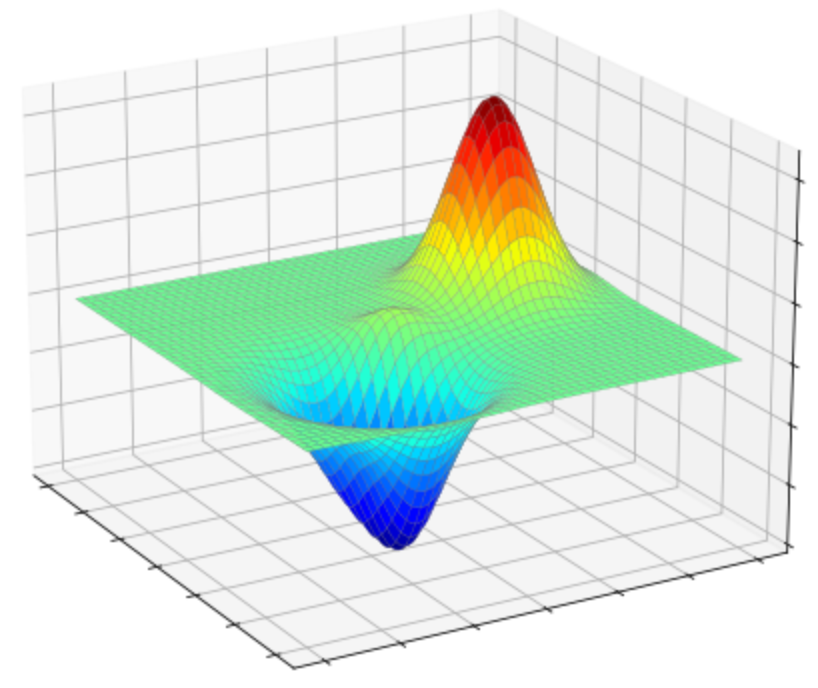
(a) Smooth objective function

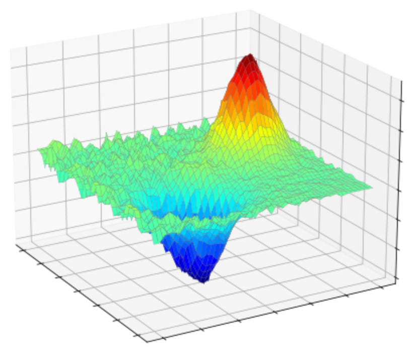
(b) Accessible function with error

Figure 2: Illustration of a smooth objective function and the accessible function that contains error.

Please note that we do not impose any other assumptions on the accessible function $f^{\prime}$. Thus, $f^{\prime}$ can be non-Lipschitz or even discontinuous. Even in such cases, we can develop an algorithm with a convergence guarantee because its smoothed function $F^{\prime}(x,t)$ is smooth as far as $t$ is sufficiently large. In the following, we denote the Lipschitz and gradient Lipschitz constant of $F^{\prime}(\cdot,t)$ as $L_{0}(t)$ and $L_{1}(t)$, respectively.

The ZOSLGH algorithm in this setting is almost the same as Algorithm 3. The only difference is $\sqrt{\nu}$ rather than $\epsilon$ in the update rule of $t_{k+1}$. See the Algorithm 4 for a more detailed description. Please note that $F^{\prime},\tilde{g}^{\prime}_{x},\tilde{G}^{\prime}_{x,u},\tilde{g}^{\prime}_{t},\tilde{G}^{\prime}_{t,v}$ are defined in the same way as the no-error setting using $f^{\prime}$.

Algorithm 4 Deterministic/Stochastic Zeroth-Order Single Loop GH algorithm (ZOSLGH) with error tolerance

0:  Iteration number $T$, initial solution $x_{1}$, initial smoothing parameter $t_{1}$, sequence of step sizes $\{\beta_{k}\}$ for $x$, step size $\eta$ for $t$, decreasing factor $\gamma\in(0,1)$, error tolerance $\nu$

  for $k=1$ to $T$ do

     Sample $u_{k}$ from $\mathcal{N}(0,\mathrm{I}_{d})$

     Update $x_{k}$ by

$$x_{k+1}=x_{k}-\beta_{k}\bar{G}^{\prime}_{x,u},$$

$$\text{where }\bar{G}^{\prime}_{x,u}=\left\{\begin{array}[]{cc}\tilde{g}^{\prime}_{x}(x_{k},t_{k};u_{k})&(\text{deterministic})\\ \tilde{G}^{\prime}_{x}(x_{k},t_{k};\xi_{k},u_{k}),\ \xi_{k}\sim P&(\text{stochastic})\end{array}\right.$$

     Sample $v_{k}$ from $\mathcal{N}(0,\mathrm{I}_{d})$

     Update $t_{k}$ by

$$t_{k+1}=\left\{\begin{array}[]{cc}\text{max}\{\gamma t_{k},\sqrt{\nu}\}&(\text{SLGH}_{\text{r}})\\ \text{max}\{\text{min}\{t_{k}-\eta\bar{G}^{\prime}_{t,v},\gamma t_{k}\},\sqrt{\nu}\}&(\text{SLGH}_{\text{d}})\end{array},\right.$$

$$\text{where }\bar{G}^{\prime}_{t,v}=\left\{\begin{array}[]{cc}\tilde{g}^{\prime}_{t}(x_{k},t_{k};v_{k})&(\text{deterministic})\\ \tilde{G}^{\prime}_{t}(x_{k},t_{k};\xi_{k},v_{k}),\ \xi_{k}\sim P&(\text{stochastic})\end{array}\right.$$

  end for

We provide the convergence analyses in the following theorems. The definitions of $\hat{x}$ in the deterministic and stochastic settings are given in Appendix C.2 and C.3, respectively.

Theorem C.1 (Convergence of ZOSLGH with error tolerance, Deterministic setting).

Suppose Assumptions A1 and A3 hold.

Take $k_{1}:=\Theta(d/\epsilon^{2})$ and $k_{2}:=O\left(\log_{\gamma}1/d\right)$ and define $k_{0}=\min\{k_{1},k_{2}\}$. Let $\hat{x}:=x_{k^{\prime}}$, where $k^{\prime}$ is chosen from a uniform distribution over $\{k_{0}+1,k_{0}+2,\ldots,T\}$. Set the stepsize for $x$ at iteration $k$ as $\beta_{k}=\frac{1}{16(d+4)L_{1}(t_{k})}\ ,k\in[T]$. Then, for any setting of the parameter $\gamma$, if the error level $\nu$ satisfies $\nu=O(\epsilon^{2}/d^{3})$, $\hat{x}$ satisfies $\mathbb{E}[\|\nabla f(\hat{x})\|]\leq\epsilon$ with the iteration complexity of $T=O({d^{3}}/{\epsilon^{2}})$, where the expectation is taken w.r.t. random vectors $\{u_{k}\}$ and $\{v_{k}\}$. Further, if we choose $\gamma\leq d^{-\Omega(\epsilon^{2}/d)}$, the iteration complexity can be bounded as $T=O({d}/{\epsilon^{2}})$.

Theorem C.2 (Convergence of ZOSLGH with error tolerance, Stochastic setting).

Suppose Assumptions A1, A2 and A3 hold. Take $k_{1}:=\Theta(d/\epsilon^{4})$ and $k_{2}:=O\left(\log_{\gamma}1/d\right)$ and define $k_{0}=\min\{k_{1},k_{2}\}$. Let $\hat{x}:=x_{k^{\prime}}$, where $k^{\prime}$ is chosen from a uniform distribution over $\{k_{0}+1,k_{0}+2,\ldots,T\}$. Set the stepsize for $x$ at iteration $k$ as $\beta_{k}=\min\left\{\frac{1}{16(d+4)L_{1}(t_{k})},\frac{1}{\sqrt{(T-k_{0})(d+4)}}\right\}$. Then, for any setting of the parameter $\gamma$, if the error level $\nu$ satisfies $\nu=O(\epsilon^{2}/d^{3})$, $\hat{x}$ satisfies $\mathbb{E}[\|\nabla f(\hat{x})\|]\leq\epsilon$ with the iteration complexity of $T=O(d^{2}/\epsilon^{4}+d^{3}/\epsilon^{2})$, where the expectation is taken w.r.t. random vectors $\{u_{k}\},\{v_{k}\}$ and $\{\xi_{k}\}$. Further, if we choose $\gamma\leq d^{-\Omega(\epsilon^{4}/d)}$, the iteration complexity can be bounded as $T=O(d/\epsilon^{4})$.

C.1 Proofs for technical lemmas

We introduce several lemmas before going to the convergence analysis. All of them describe properties of the function with error $f^{\prime}$ and its Gaussian smoothing $F^{\prime}$. Throughout this subsection, we assume that $f$ is $L_{0}$-Lipschitz and $L_{1}$-smooth function. We also suppose that the function pair $(f,f^{\prime})$ satisfies $\mathop{\rm sup}\limits_{x\in\mathbb{R}^{d}}|f(x)-f^{\prime}(x)|\leq\nu$.

Lemma C.3.

For any $x\in\mathbb{R}^{d}$ and $t>0$, we have

$$\mathbb{E}_{u}\left[\frac{1}{t^{2}}(f^{\prime}(x+tu)-f^{\prime}(x))^{2}\|u\|^{2}\right]\leq 4(d+4)\|\nabla f(x)\|^{2}+t^{2}L_{1}^{2}(d+6)^{3}+8d\frac{\nu^{2}}{t^{2}}.$$

Proof:

$$\mathbb{E}_{u}\left[\frac{1}{t^{2}}(f^{\prime}(x+tu)-f^{\prime}(x))^{2}\|u\|^{2}\right] =\mathbb{E}_{u}\left[\frac{1}{t^{2}}(f(x+tu)-f(x)+(f^{\prime}-f)(x+tu)-(f^{\prime}-f)(x))^{2}\|u\|^{2}\right]$$

$$\leq 2\mathbb{E}_{u}\left[\frac{1}{t^{2}}(f(x+tu)-f(x))^{2}\|u\|^{2}\right]+2\mathbb{E}_{u}\left[\frac{1}{t^{2}}(2\nu)^{2}\|u\|^{2}\right]$$

$$\leq 4(d+4)\|\nabla f(x)\|^{2}+t^{2}L_{1}^{2}(d+6)^{3}+8d\frac{\nu^{2}}{t^{2}},$$

where the last inequality holds due to Lemma B.1 and Lemma B.4.

Lemma C.4.

For any $x\in\mathbb{R}^{d}$ and $t>0$, we have

$$\mathbb{E}_{\zeta}\left[\frac{1}{t^{2}}(\bar{f}^{\prime}(x+tu;\xi)-\bar{f}^{\prime}(x;\xi))^{2}\|u\|^{2}\right]\leq 4(d+4)(\|\nabla f(x)\|^{2}+\sigma^{2})+t^{2}L_{1}^{2}(d+6)^{3}+8d\frac{\nu^{2}}{t^{2}}.$$

Proof:

$$\mathbb{E}_{\zeta}\left[\frac{1}{t^{2}}(\bar{f}^{\prime}(x+tu;\xi)-\bar{f}^{\prime}(x;\xi))^{2}\|u\|^{2}\right]$$

$$=\mathbb{E}_{\xi}\left[\mathbb{E}_{u}\left[\frac{1}{t^{2}}(\bar{f}(x+tu;\xi)-\bar{f}(x;\xi)+(\bar{f}^{\prime}-\bar{f})(x+tu;\xi)-(\bar{f}^{\prime}-\bar{f})(x;\xi))^{2}\|u\|^{2}\right]\right]$$

$$\leq 2\mathbb{E}_{\xi}\left[\mathbb{E}_{u}\left[\frac{1}{t^{2}}(\bar{f}(x+tu;\xi)-\bar{f}(x;\xi))^{2}\|u\|^{2}\right]\right]+\frac{2}{t^{2}}\mathbb{E}_{\xi}[\mathbb{E}_{u}[(2\nu)^{2}\|u\|^{2}]]$$

$$\leq 2\mathbb{E}_{\xi}\left[\frac{t^{2}}{2}L_{1}^{2}(d+6)^{3}+2(d+4)\|\nabla\bar{f}(x;\xi)\|^{2}\right]+8d\frac{\nu^{2}}{t^{2}}$$

$$\leq 4(d+4)(\|\nabla f(x)\|^{2}+\sigma^{2})+t^{2}L_{1}^{2}(d+6)^{3}+8d\frac{\nu^{2}}{t^{2}},$$

where the second inequality follows from Lemma B.1 and Lemma B.4, and the last inequality holds due to Assumption A2 (ii).

Lemma C.5.

For any $x\in\mathbb{R}^{d}$ and for any $t_{1},t_{2}\in\mathcal{T}$, we have

$$|F^{\prime}(x,t_{1})-F^{\prime}(x,t_{2})|\leq L_{0}|t_{1}-t_{2}|\sqrt{d}+2\nu.$$

Proof:

$$|F^{\prime}(x,t_{1})-F^{\prime}(x,t_{2})| =|F(x,t_{1})-F(x,t_{2})+(F^{\prime}-F)(x,t_{1})-(F^{\prime}-F)(x,t_{2})|$$

$$\leq|F(x,t_{1})-F(x,t_{2})|+|\mathbb{E}_{u}[(f^{\prime}-f)(x+t_{1}u)]|+|\mathbb{E}_{u}[(f^{\prime}-f)(x+t_{2}u)]|$$

$$\leq|F(x,t_{1})-F(x,t_{2})|+\mathbb{E}_{u}[|(f^{\prime}-f)(x+t_{1}u)|]+\mathbb{E}_{u}[|(f^{\prime}-f)(x+t_{2}u)|]$$

$$\leq|F(x,t_{1})-F(x,t_{2})|+2\nu$$

$$\leq L_{0}|t_{1}-t_{2}|\sqrt{d}+2\nu,$$

where the last inequality holds due to Lemma 3.3.

Lemma C.6 (Lemma 30 in [Jin et al. (2018)]).

For any $x\in\mathbb{R}^{d}$ and for any $t_{1},t_{2}\in\mathcal{T}$, we have

$$\|\nabla_{x}(F^{\prime}-F)(x,t)\|\leq\sqrt{\frac{2}{\pi}}\frac{\nu}{t}.$$

Lemma C.7.

(i) $F^{\prime}(x,t)$ is $L_{0}+\sqrt{\frac{2}{\pi}}\frac{\nu}{t}$-Lipschitz in terms of $x$.
(ii) (Lemma 20 in [Jin et al. (2018)]) $F^{\prime}(x,t)$ is $L_{1}+\frac{2\nu}{t^{2}}$-smooth in terms of $x$.

Proof for (i):

$$\|\nabla_{x}F^{\prime}(x,t)\| \leq\|\nabla_{x}F(x,t)\|+\|\nabla_{x}(F^{\prime}-F)(x,t)\|$$

$$\leq L_{0}+\sqrt{\frac{2}{\pi}}\frac{\nu}{t},$$

where the last inequality holds due to Lemma 3.2 and Lemma C.6.

Lemma C.8.

For any $x\in\mathbb{R}^{d}$ and $t>0$, we have

$$\|\nabla f(x)\|^{2}\leq 4\|\nabla_{x}F^{\prime}(x,t)\|^{2}+\frac{t^{2}}{2}L_{1}^{2}(d+6)^{3}+\frac{8}{\pi}\frac{\nu^{2}}{t^{2}}.$$

Proof: We have

$$\|\nabla f(x)\|^{2} =\|\mathbb{E}_{u}[\langle\nabla f(x),u\rangle u]\|^{2}$$

$$=\left\|\frac{1}{t}\mathbb{E}_{u}[(f(x+tu)-f(x)-[f(x+tu)-f(x)-t\langle\nabla f(x),u\rangle])u]\right\|^{2}$$

$$\leq\left\|\nabla_{x}F(x,t)-\frac{1}{t}\mathbb{E}_{u}[(f(x+tu)-f(x)-t\langle\nabla f(x),u\rangle)u]\right\|^{2}$$

$$\leq 2\|\nabla_{x}F(x,t)\|^{2}+\frac{2}{t^{2}}\left\|\mathbb{E}_{u}[(f(x+tu)-f(x)-t\langle\nabla f(x),u\rangle)u]\right\|^{2}$$

$$\leq 2\|\nabla_{x}F(x,t)\|^{2}+\frac{2}{t^{2}}\mathbb{E}_{u}[|f(x+tu)-f(x)-t\langle\nabla f(x),u\rangle|^{2}\|u\|^{2}]$$

$$\leq 2\|\nabla_{x}F(x,t)\|^{2}+\frac{t^{2}L_{1}^{2}}{2}\mathbb{E}_{u}[\|u\|^{6}]$$

$$\leq 2\|\nabla_{x}F(x,t)\|^{2}+\frac{t^{2}L_{1}^{2}}{2}(d+6)^{3}$$

$$\leq 2(2\|\nabla_{x}(F-F^{\prime})(x,t)\|^{2}+2\|\nabla_{x}F^{\prime}(x,t)\|^{2})+\frac{t^{2}L_{1}^{2}}{2}(d+6)^{3}$$

$$\leq 4\|\nabla_{x}F^{\prime}(x,t)\|^{2}+\frac{t^{2}L_{1}^{2}}{2}(d+6)^{3}+\frac{8}{\pi}\frac{\nu^{2}}{t^{2}},$$

where the third last inequality holds due to Lemma B.1, and the last inequality holds due to Lemma C.6.

C.2 Proof for the deterministic setting

Proof for Theorem C.1: Let $w_{k}:=(u_{k},v_{k})$ and denote $\delta_{k}:=\tilde{g}^{\prime}_{x}(x_{k},t_{k};u_{k})-\nabla_{x}F^{\prime}(x_{k},t_{k})$. Utilize the updating rule for $x$ and $L_{1}(t)$-smoothness of $F^{\prime}(\cdot,t)$. Then we have

$$F^{\prime}(x_{k+1},t_{k}) \leq F^{\prime}(x_{k},t_{k})+\left<\nabla_{x}F^{\prime}(x_{k},t_{k}),(x_{k+1}-x_{k})\right>+\frac{L_{1}(t_{k})}{2}\|x_{k+1}-x_{k}\|^{2}$$

$$=F^{\prime}(x_{k},t_{k})-\beta_{k}\left<\nabla_{x}F^{\prime}(x_{k},t_{k}),\tilde{g}^{\prime}_{x}(x_{k},t_{k};u_{k})\right>+\frac{L_{1}(t_{k})}{2}\beta_{k}^{2}\|\tilde{g}^{\prime}_{x}(x_{k},t_{k};u_{k})\|^{2}$$

$$=F^{\prime}(x_{k},t_{k})-\beta_{k}\|\nabla_{x}F^{\prime}(x_{k},t_{k})\|^{2}-\beta_{k}\left<\nabla_{x}F^{\prime}(x_{k},t_{k}),\delta_{k}\right>+\frac{L_{1}(t_{k})}{2}\beta_{k}^{2}\|\tilde{g}^{\prime}_{x}(x_{k},t_{k};u_{k}))\|^{2}.$$ (26)

Denote

$$E_{k}:=-\beta_{k}\left<\nabla_{x}F^{\prime}(x_{k},t_{k}),\delta_{k}\right>+\frac{L_{1}(t_{k})}{2}\beta_{k}^{2}\|\tilde{g}^{\prime}_{x}(x_{k},t_{k};u_{k})\|^{2}$$

for simplicity. From Lemma C.5 and (26), we get the upper bound for $\|\nabla_{x}F^{\prime}(x,t)\|^{2}$ as

$$\beta_{k}\|\nabla_{x}F^{\prime}(x_{k},t_{k})\|^{2} \leq F^{\prime}(x_{k},t_{k})-F^{\prime}(x_{k+1},t_{k})+E_{k}$$

$$=F^{\prime}(x_{k},t_{k})-F^{\prime}(x_{k+1},t_{k+1})+F^{\prime}(x_{k+1},t_{k+1})-F^{\prime}(x_{k+1},t_{k})+E_{k}$$

$$\leq F^{\prime}(x_{k},t_{k})-F^{\prime}(x_{k+1},t_{k+1})+L_{0}|t_{k+1}-t_{k}|\sqrt{d}+2\nu+E_{k}.$$

Now, sum up the above inequality for all iterations $k_{0}+1\leq k\leq T\ (T>k_{0})$. Then we have

$$\sum_{k=k_{0}+1}^{T}\beta_{k}\|\nabla_{x}F^{\prime}(x_{k},t_{k})\|^{2}$$

$$\leq F^{\prime}(x_{k_{0}+1},t_{k_{0}+1})-F^{\prime}(x_{T+1},t_{T+1})+L_{0}\sum_{k=k_{0}+1}^{T}|t_{k+1}-t_{k}|\sqrt{d}+2\nu(T-k_{0})+\sum_{k=k_{0}+1}^{T}E_{k}$$

$$\leq F^{\prime}(x_{k_{0}+1},t_{k_{0}+1})-f^{*}+\nu+L_{0}\sqrt{d}\sum_{k=k_{0}+1}^{T}|t_{k+1}-t_{k}|+2\nu(T-k_{0})+\sum_{k=k_{0}+1}^{T}E_{k}.$$

$$\leq f^{\prime}(x_{k_{0}+1})-f^{*}+3\nu+L_{0}\sqrt{d}\left(t_{k_{0}+1}+\sum_{k=k_{0}+1}^{T}|t_{k+1}-t_{k}|\right)+2\nu(T-k_{0})+\sum_{k=k_{0}+1}^{T}E_{k}$$

$$\leq f(x_{k_{0}+1})-f^{*}+4\nu+L_{0}\sqrt{d}\left(t_{k_{0}+1}+\sum_{k=k_{0}+1}^{T}|t_{k+1}-t_{k}|\right)+2\nu(T-k_{0})+\sum_{k=k_{0}+1}^{T}E_{k},$$ (27)

where the third inequality holds due to Lemma C.5. We can bound the conditional expectation of $E_{k}$ as

$$\mathbb{E}_{w_{k}}[E_{k}\mid w_{[k-1]}]$$

$$=-\beta_{k}\mathbb{E}_{w_{k}}[\left<\nabla_{x}F^{\prime}(x_{k},t_{k}),\delta_{k}\right>\mid w_{[k-1]}]+\frac{\mathbb{E}_{w_{k}}[L_{1}(t_{k})\mid w_{[k-1]}]}{2}\beta_{k}^{2}\mathbb{E}_{w_{k}}[\|\tilde{g}^{\prime}_{x}(x_{k},t_{k};u_{k})\|^{2}\mid w_{[k-1]}]$$

$$\leq\frac{\mathbb{E}_{w_{k}}[L_{1}(t_{k})\mid w_{[k-1]}]}{2}\beta_{k}^{2}\mathbb{E}_{w_{k}}[\|\tilde{g}^{\prime}_{x}(x_{k},t_{k};u_{k})\|^{2}\mid w_{[k-1]}]$$

$$\leq\frac{\mathbb{E}_{w_{k}}[L_{1}(t_{k})\mid w_{[k-1]}]}{2}\beta_{k}^{2}\left(4(d+4)\mathbb{E}_{w_{k}}[\|\nabla f(x_{k})\|^{2}\mid w_{[k-1]}]+L_{1}^{2}(d+6)^{3}\mathbb{E}_{w_{k}}[t_{k}^{2}\mid w_{[k-1]}]\right.$$

$$\left.\hskip 113.81102pt+8d\mathbb{E}_{w_{k}}\left[\nu^{2}/t_{k}^{2}\mid w_{[k-1]}\right]\right),$$

where the first inequality holds since we have $\mathbb{E}_{w_{k}}[\delta_{k}\mid w_{[k-1]}]=\mathbb{E}_{u_{k}}[\delta_{k}\mid u_{[k-1]}]=0$, and the last inequality holds due to Lemma C.3. Take the expectations of (27) w.r.t. random vectors $\{w_{k_{0}+1},...,w_{T}\}$. Then we can get

$$\sum_{k=k_{0}+1}^{T}\beta_{k}\mathbb{E}_{w}[\|\nabla_{x}F^{\prime}(x_{k},t_{k})\|^{2}]$$

$$\leq f(x_{k_{0}+1})-f^{*}+4\nu+L_{0}\sqrt{d}\left(t_{k_{0}+1}+\sum_{k=k_{0}+1}^{T}\mathbb{E}_{w}[|t_{k+1}-t_{k}|]\right)+2\nu(T-k_{0})$$

$$+\frac{1}{2}\left(4(d+4)\sum_{k=k_{0}+1}^{T}\beta_{k}^{2}\mathbb{E}_{w}[L_{1}(t_{k})\|\nabla f(x_{k})\|^{2}]+L_{1}^{2}(d+6)^{3}\sum_{k=k_{0}+1}^{T}\beta_{k}^{2}\mathbb{E}_{w}[L_{1}(t_{k})t_{k}^{2}]\right.$$

$$\left.\hskip 24.18483pt+8d\sum_{k=k_{0}+1}^{T}\beta_{k}^{2}\mathbb{E}_{w}\left[L_{1}(t_{k})\frac{\nu^{2}}{t_{k}^{2}}\right]\right).$$ (28)

Lemma C.8 together with (28) yields

$$\sum_{k=k_{0}+1}^{T}\beta_{k}\mathbb{E}_{w}[\|\nabla f(x_{k})\|^{2}]$$

$$\leq 4\sum_{k=k_{0}+1}^{T}\beta_{k}\mathbb{E}_{w}[\|\nabla_{x}F^{\prime}(x_{k},t_{k})\|^{2}]+\frac{1}{2}\sum_{k=k_{0}+1}^{T}\beta_{k}\mathbb{E}_{w}[t_{k}^{2}]L_{1}^{2}(d+6)^{3}+\frac{8}{\pi}\sum_{k=k_{0}+1}^{T}\beta_{k}\mathbb{E}_{w}\left[\frac{\nu^{2}}{t_{k}^{2}}\right]$$

$$\leq 4\left(f(x_{k_{0}+1})-f^{*}+4\nu+L_{0}\sqrt{d}\left(t_{k_{0}+1}+\sum_{k=k_{0}+1}^{T}\mathbb{E}_{w}[|t_{k+1}-t_{k}|]\right)+2\nu(T-k_{0})\right)$$

$$+2\left(4(d+4)\sum_{k=k_{0}+1}^{T}\beta_{k}^{2}\mathbb{E}_{w}[L_{1}(t_{k})\|\nabla f(x_{k})\|^{2}]+L_{1}^{2}(d+6)^{3}\sum_{k=k_{0}+1}^{T}\beta_{k}^{2}\mathbb{E}_{w}[L_{1}(t_{k})t_{k}^{2}]\right.$$

$$\left.\hskip 24.18483pt+8d\sum_{k=k_{0}+1}^{T}\beta_{k}^{2}\mathbb{E}_{w}\left[L_{1}(t_{k})\frac{\nu^{2}}{t_{k}^{2}}\right]\right)$$

$$+\frac{1}{2}\sum_{k=k_{0}+1}^{T}\beta_{k}\mathbb{E}_{w}[t_{k}^{2}]L_{1}^{2}(d+6)^{3}+\frac{8}{\pi}\sum_{k=k_{0}+1}^{T}\beta_{k}\mathbb{E}_{w}\left[\frac{\nu^{2}}{t_{k}^{2}}\right].$$

By rearranging the terms, we obtain

$$\sum_{k=k_{0}+1}^{T}\left(\beta_{k}\mathbb{E}_{w}[\|\nabla f(x_{k})\|^{2}]-8(d+4)\beta_{k}^{2}\mathbb{E}_{w}[L_{1}(t_{k})\|\nabla f(x_{k})\|^{2}]\right)$$

$$\leq 4\left(f(x_{k_{0}+1})-f^{*}+4\nu+L_{0}\sqrt{d}\left(t_{k_{0}+1}+\sum_{k=k_{0}+1}^{T}\mathbb{E}_{w}[|t_{k+1}-t_{k}|]\right)+2\nu(T-k_{0})\right)$$

$$+2\left(L_{1}^{2}(d+6)^{3}\sum_{k=k_{0}+1}^{T}\beta_{k}^{2}\mathbb{E}_{w}[L_{1}(t_{k})t_{k}^{2}]+8d\sum_{k=k_{0}+1}^{T}\beta_{k}^{2}\mathbb{E}_{w}\left[L_{1}(t_{k})\frac{\nu^{2}}{t_{k}^{2}}\right]\right)$$

$$+\frac{1}{2}\sum_{k=k_{0}+1}^{T}\beta_{k}\mathbb{E}_{w}[t_{k}^{2}]L_{1}^{2}(d+6)^{3}+\frac{8}{\pi}\sum_{k=k_{0}+1}^{T}\beta_{k}\mathbb{E}_{w}\left[\frac{\nu^{2}}{t_{k}^{2}}\right].$$ (29)

If we update $t_{k}\ (k\in[T])$ as in Algorithm 4, we have $\nu=O(t_{k}^{2})$, which yields $L_{1}(t_{k})=O(1)$ from Lemma C.7. Hence, by setting the step size $\beta_{k}$ as $\frac{1}{16(d+4)L_{1}(t_{k})}\ (k\in[T])$, we can obtain

$$\frac{1}{T-k_{0}}\sum_{k=k_{0}+1}^{T}\mathbb{E}_{w}[\|\nabla f(x_{k})\|^{2}] =O\left(\frac{d}{T-k_{0}}\left(1+\sqrt{d}\sum_{k=k_{0}+1}^{T}\mathbb{E}_{w}[|t_{k+1}-t_{k}|]+d^{2}\sum_{k=k_{0}+1}^{T}\mathbb{E}_{w}[t_{k}^{2}]\right)\right)$$

in the same way as before. We can also get $\sum_{k=k_{0}+1}^{T}|t_{k+1}-t_{k}|=\sum_{k=k_{0}+1}^{T}(t_{k}-t_{k+1})=t_{k_{0}+1}-t_{T+1}=t_{k_{0}+1}=O(\gamma^{k_{0}})$. Further, we have

$$\sum_{k=k_{0}+1}^{T}t_{k}^{2}\leq\sum_{k=k_{0}+1}^{T}\max\{t_{1}^{2}\gamma^{2(k-1)},\nu\}\leq\sum_{k=k_{0}+1}^{T}\left(t_{1}^{2}\gamma^{2(k-1)}+\nu\right) \leq\frac{t_{1}^{2}\gamma^{2k_{0}}}{1-\gamma^{2}}+\nu(T-k_{0})$$

$$=O(\gamma^{2k_{0}}+\nu(T-k_{0})),$$

where the first inequality follows from the update rule of $t_{k}$ in Algorithm 4. Hence, we obtain

$$\frac{1}{T-k_{0}}\sum_{k=k_{0}+1}^{T}\mathbb{E}_{w}[\|\nabla f(x_{k})\|^{2}] =O\left(\frac{d}{T-k_{0}}\left(1+\sqrt{d}\gamma^{k_{0}}+d^{2}(\gamma^{2k_{0}}+\nu(T-k_{0}))\right)\right)$$

$$=O\left(\frac{d(1+d^{2}\gamma^{2k_{0}})}{T-k_{0}}+d^{3}\nu\right)=O\left(\frac{d(1+d^{2}\gamma^{2k_{0}})}{T-k_{0}}+\epsilon^{2}\right),$$

where the last equality follows from the assumption of $\nu=O(\epsilon^{2}/d^{3})$.

Here, we have $k_{0}=O\left(\frac{d}{\epsilon^{2}}\right)$ by the definition of $k_{0}$. Thus, by setting $T=k_{0}+O\left(\frac{d^{3}}{\epsilon^{2}}\right)=O\left(\frac{d^{3}}{\epsilon^{2}}\right)$, we can obtain $\mathbb{E}_{w,k^{\prime}}[\|\nabla f(\hat{x})\|^{2}]=\frac{1}{T-k_{0}}\sum_{k=k_{0}+1}^{T}\mathbb{E}_{w}[\|\nabla f(x_{k})\|^{2}]\leq\epsilon^{2}$. This implies $\mathbb{E}_{w,k^{\prime}}[\|\nabla f(\hat{x})\|]\leq\epsilon$ as $\mathbb{E}_{w,k^{\prime}}[\|\nabla f(\hat{x})\|]^{2}\leq\mathbb{E}_{w,k^{\prime}}[\|\nabla f(\hat{x})\|^{2}]$ follows from Jensen’s inequality. Furthermore, when $\gamma$ is chosen as $\gamma\leq d^{-\epsilon^{2}/d}$ , we have $\log_{\gamma}d^{-1}=O\left(\frac{d}{\epsilon^{2}}\right)$, which implies $k_{0}=\Omega\left(\log_{\gamma}d^{-1}\right)$. Therefore, we can obtain $\gamma^{k_{0}}=O(d^{-1})$, which yields the iteration complexity of $T=O\left(\frac{d}{\epsilon^{2}}\right)$.

$\Box$

C.3 Proof for the stochastic setting

Proof for Theorem C.2:

Let $\zeta_{k}:=(\xi_{k},u_{k},v_{k})$, $k\in[T]$ and denote $\delta_{k}:=\tilde{G}^{\prime}_{x}(x_{k},t_{k};\xi_{k},u_{k})-\nabla_{x}F^{\prime}(x_{k},t_{k}).$ Since $\tilde{G}^{\prime}_{x}(x,t;\xi,u)$ is an unbiased estimator of $\nabla_{x}F^{\prime}(x,t)$, we have

$$F^{\prime}(x_{k+1},t_{k}) \leq F^{\prime}(x_{k},t_{k})+\left<\nabla_{x}F^{\prime}(x_{k},t_{k}),(x_{k+1}-x_{k})\right>+\frac{L_{1}(t_{k})}{2}\|x_{k+1}-x_{k}\|^{2}$$

$$=F^{\prime}(x_{k},t_{k})-\beta_{k}\left<\nabla_{x}F^{\prime}(x_{k},t_{k}),\tilde{G}^{\prime}_{x}(x_{k},t_{k};\xi_{k},u_{k})\right>+\frac{L_{1}(t_{k})}{2}\beta_{k}^{2}\|\tilde{G}^{\prime}_{x}(x_{k},t_{k};\xi_{k},u_{k})\|^{2}$$

$$=F^{\prime}(x_{k},t_{k})-\beta_{k}\|\nabla_{x}F^{\prime}(x_{k},t_{k})\|^{2}-\beta_{k}\left<\nabla_{x}F^{\prime}(x_{k},t_{k}),\delta_{k}\right>+\frac{L_{1}(t_{k})}{2}\beta_{k}^{2}\|\tilde{G}^{\prime}_{x}(x_{k},t_{k};\xi_{k},u_{k})\|^{2}.$$

Now, denote

$$I_{k}:=-\beta_{k}\left<\nabla_{x}F^{\prime}(x_{k},t_{k}),\delta_{k}\right>+\frac{L_{1}(t_{k})}{2}\beta_{k}^{2}\|\tilde{G}^{\prime}_{x}(x_{k},t_{k};\xi_{k},u_{k})\|^{2}$$

for simplicity. Then, we can get the upper bound for $\|\nabla_{x}F(x,t)\|^{2}$ with $I_{k}$:

$$\beta_{k}\|\nabla_{x}F^{\prime}(x_{k},t_{k})\|^{2} \leq F^{\prime}(x_{k},t_{k})-F^{\prime}(x_{k+1},t_{k})+I_{k}$$

$$=F^{\prime}(x_{k},t_{k})-F^{\prime}(x_{k+1},t_{k+1})+F^{\prime}(x_{k+1},t_{k+1})-F^{\prime}(x_{k+1},t_{k})+I_{k}$$

$$\leq F^{\prime}(x_{k},t_{k})-F^{\prime}(x_{k+1},t_{k+1})+L_{0}|t_{k+1}-t_{k}|\sqrt{d}+2\nu+I_{k},$$

where the last inequality follows from Lemma C.5. Sum up the above inequality for all iterations $k_{0}+1\leq k\leq T$. Then we have

$$\sum_{k=k_{0}+1}^{T}\beta_{k}\|\nabla_{x}F^{\prime}(x_{k},t_{k})\|^{2}$$

$$\leq F^{\prime}(x_{k_{0}+1},t_{k_{0}+1})-F^{\prime}(x_{T+1},t_{T+1})+L_{0}\sqrt{d}\sum_{k=k_{0}+1}^{T}|t_{k+1}-t_{k}|+2\nu(T-k_{0})+\sum_{k=k_{0}+1}^{T}I_{k}$$

$$\leq f(x_{k_{0}+1})-f^{*}+4\nu+L_{0}\sqrt{d}\left(t_{k_{0}+1}+\sum_{k=k_{0}+1}^{T}|t_{k+1}-t_{k}|\right)+2\nu(T-k_{0})+\sum_{k=k_{0}+1}^{T}I_{k}.$$ (30)

We can also obtain

$$\mathbb{E}_{\zeta_{k}}[I_{k}\mid\zeta_{[k-1]}]$$

$$=-\beta_{k}\mathbb{E}_{\zeta_{k}}[\left<\nabla_{x}F^{\prime}(x_{k},t_{k}),\delta_{k}\right>\mid\zeta_{[k-1]}]+\frac{\mathbb{E}_{\zeta_{k}}[L_{1}(t_{k})\mid\zeta_{[k-1]}]}{2}\beta_{k}^{2}\mathbb{E}_{\zeta_{k}}[\|\tilde{G}^{\prime}_{x}(x_{k},t_{k};\xi_{k},u_{k})\|^{2}\mid\zeta_{[k-1]}]$$

$$=\frac{\mathbb{E}_{\zeta_{k}}[L_{1}(t_{k})\mid\zeta_{[k-1]}]}{2}\beta_{k}^{2}\mathbb{E}_{\zeta_{k}}[\|\tilde{G}^{\prime}_{x}(x_{k},t_{k};\xi_{k},u_{k})\|^{2}\mid\zeta_{[k-1]}]$$

$$\leq\frac{\mathbb{E}_{\zeta_{k}}[L_{1}(t_{k})\mid\zeta_{[k-1]}]s}{2}\beta_{k}^{2}\left(4(d+4)(\mathbb{E}_{\zeta_{k}}[\|\nabla f(x_{k})\|^{2}\mid\zeta_{[k-1]}]+\sigma^{2})+\mathbb{E}_{\zeta_{k}}[t_{k}^{2}\mid\zeta_{[k-1]}]L_{1}^{2}(d+6)^{3}\right.$$

$$\left.\hskip 113.24197pt+8d\mathbb{E}_{\zeta_{k}}\left[\nu^{2}/t_{k}^{2}\mid\zeta_{[k-1]}\right]\right),$$

where the last inequality holds due to Lemma C.4.

Take the expectation of (30) with respect to $\zeta_{k_{0}+1},\ldots,\zeta_{T}$. Then we have

$$\sum_{k=k_{0}+1}^{T}\beta_{k}\mathbb{E}_{\zeta}[\|\nabla_{x}F^{\prime}(x_{k},t_{k})\|^{2}]$$

$$\leq f(x_{k_{0}+1})-f^{*}+4\nu+L_{0}\sqrt{d}\left(t_{k_{0}+1}+\sum_{k=k_{0}+1}^{T}\mathbb{E}_{\zeta}[|t_{k+1}-t_{k}|]\right)+2\nu(T-k_{0})+\sum_{k=k_{0}+1}^{T}\mathbb{E}_{\zeta}[I_{k}]$$

$$\leq f(x_{k_{0}+1})-f^{*}+4\nu+L_{0}\sqrt{d}\left(t_{k_{0}+1}+\sum_{k=k_{0}+1}^{T}\mathbb{E}_{\zeta}[|t_{k+1}-t_{k}|]\right)+2\nu(T-k_{0})+$$

$$+\frac{1}{2}\left(4(d+4)\sum_{k=k_{0}+1}^{T}\beta_{k}^{2}(\mathbb{E}_{\zeta}[L_{1}(t_{k})\|\nabla f(x_{k})\|^{2}]+\sigma^{2})+L_{1}^{2}(d+6)^{3}\sum_{k=k_{0}+1}^{T}\beta_{k}^{2}\mathbb{E}_{\zeta}[L_{1}(t_{k})t_{k}^{2}]\right.$$

$$\left.\hskip 24.18483pt+8d\sum_{k=k_{0}+1}^{T}\beta_{k}^{2}\mathbb{E}_{\zeta}\left[L_{1}(t_{k})\frac{\nu^{2}}{t_{k}^{2}}\right]\right),$$

From Lemma C.8 (ii), we have

$$\sum_{k=k_{0}+1}^{T}\beta_{k}\mathbb{E}_{\zeta}[\|\nabla f(x_{k})\|^{2}]$$

$$\leq 4\sum_{k=k_{0}+1}^{T}\beta_{k}\mathbb{E}_{\zeta}[\|\nabla_{x}F^{\prime}(x_{k},t_{k})\|^{2}]+\frac{L_{1}^{2}(d+6)^{3}}{2}\sum_{k=k_{0}+1}^{T}\beta_{k}\mathbb{E}_{\zeta}[t_{k}^{2}]+\frac{8}{\pi}\sum_{k=k_{0}+1}^{T}\beta_{k}\mathbb{E}_{\zeta}\left[\frac{\nu^{2}}{t_{k}^{2}}\right]$$

$$\leq 4\left(f(x_{k_{0}+1})-f^{*}+4\nu+L_{0}\sqrt{d}\left(t_{k_{0}+1}+\sum_{k=k_{0}+1}^{T}\mathbb{E}_{\zeta}[|t_{k+1}-t_{k}|]\right)+2\nu(T-k_{0})\right)$$

$$+2\left(4(d+4)\sum_{k=k_{0}+1}^{T}(\beta_{k}^{2}\mathbb{E}_{\zeta}[L_{1}(t_{k})(\|\nabla f(x_{k})\|^{2}+\sigma^{2})])+L_{1}^{2}(d+6)^{3}\sum_{k=k_{0}+1}^{T}\mathbb{E}_{\zeta}\beta_{k}^{2}[L_{1}(t_{k})t_{k}^{2}]\right.$$

$$\left.\hskip 21.33955pt+8d\sum_{k=k_{0}+1}^{T}\beta_{k}^{2}\mathbb{E}_{\zeta}\left[L_{1}(t_{k})\frac{\nu^{2}}{t_{k}^{2}}\right]\right)$$

$$+\frac{L_{1}^{2}(d+6)^{3}}{2}\sum_{k=k_{0}+1}^{T}\beta_{k}\mathbb{E}_{\zeta}[t_{k}^{2}]+\frac{8}{\pi}\sum_{k=k_{0}+1}^{T}\beta_{k}\mathbb{E}_{\zeta}\left[\frac{\nu^{2}}{t_{k}^{2}}\right].$$ (31)

By rearranging the terms, we obtain

$$\sum_{k=k_{0}+1}^{T}\left(\beta_{k}\mathbb{E}_{\zeta}[\|\nabla f(x_{k})\|^{2}]-8(d+4)\beta_{k}^{2}\mathbb{E}_{\zeta}[L_{1}(t_{k})\|\nabla f(x_{k})\|^{2}]\right)$$

$$\leq 4\left(f(x_{k_{0}+1})-f^{*}+4\nu+L_{0}\sqrt{d}\left(t_{k_{0}+1}+\sum_{k=k_{0}+1}^{T}\mathbb{E}_{\zeta}[|t_{k+1}-t_{k}|]\right)+2\nu(T-k_{0})\right)$$

$$+2\left(4(d+4)\sigma^{2}\sum_{k=k_{0}+1}^{T}\beta_{k}^{2}\mathbb{E}_{\zeta}[L_{1}(t_{k})]+L_{1}^{2}(d+6)^{3}\sum_{k=k_{0}+1}^{T}\beta_{k}\mathbb{E}_{\zeta}[L_{1}(t_{k})t_{k}^{2}]+8d\sum_{k=k_{0}+1}^{T}\beta_{k}\mathbb{E}_{\zeta}\left[L_{1}(t_{k})\frac{\nu^{2}}{t_{k}^{2}}\right]\right)$$

$$+\frac{L_{1}^{2}(d+6)^{3}}{2}\sum_{k=k_{0}+1}^{T}\beta_{k}\mathbb{E}_{\zeta}[t_{k}^{2}]+\frac{8}{\pi}\sum_{k=k_{0}+1}^{T}\beta_{k}\mathbb{E}_{\zeta}\left[\frac{\nu^{2}}{t_{k}^{2}}\right].$$ (32)

If we update $t_{k}\ (k\in[T])$ as in Algorithm 4, we have $\nu=O(t_{k}^{2})$, which yields $L_{1}(t_{k})=O(1)$ from Lemma C.7. Furthermore, if we set the step size $\beta_{k}$ as $\min\left\{\frac{1}{16(d+4)L_{1}(t_{k})},\frac{1}{\sqrt{(T-k_{0})(d+4)}}\right\}\ (k\in[T])$, then we have

$$\frac{1}{\beta_{k}-8(d+4)L_{1}(t_{k})\beta_{k}^{2}}\leq\frac{2}{\beta_{k}},$$

$$\frac{1}{\beta_{k}}\leq 16(d+4)L_{1}(t_{k})+\sqrt{(T-k_{0})(d+4)}.$$

for all $k\in[T]$. Using the above inequalities, we can obtain

$$\frac{1}{T-k_{0}}\sum_{k=k_{0}+1}^{T}\mathbb{E}_{\zeta}[\|\nabla f(x_{k})\|^{2}] =O\left(\frac{\sqrt{d}\left(1+\sqrt{d}\sum_{k=k_{0}+1}^{T}\mathbb{E}_{\zeta}[|t_{k+1}-t_{k}|]\right)}{\sqrt{T-k_{0}}}+\frac{d\left(1+d^{2}\sum_{k=k_{0}+1}^{T}\mathbb{E}_{\zeta}[t_{k}^{2}]\right)}{T-k_{0}}\right)$$

$$=O\left(\frac{\sqrt{d}+d\gamma^{k_{0}}}{\sqrt{T-k_{0}}}+\frac{d+d^{3}\gamma^{2k_{0}}}{T-k_{0}}+d^{3}\nu\right)$$

$$=O\left(\frac{\sqrt{d}+d\gamma^{k_{0}}}{\sqrt{T-k_{0}}}+\frac{d+d^{3}\gamma^{2k_{0}}}{T-k_{0}}+\epsilon^{2}\right),$$

where the second and last equality can be shown via a similar way as in the proof of Theorem C.1.

Here, we have $k_{0}=O\left(\frac{d}{\epsilon^{4}}\right)$ by the definition of $k_{0}$. Thus, by setting $T=O\left(\frac{d^{3}}{\epsilon^{2}}+\frac{d^{2}}{\epsilon^{4}}\right)=O\left(\frac{d^{3}}{\epsilon^{2}}+\frac{d^{2}}{\epsilon^{4}}\right)$, we can obtain $\mathbb{E}_{\zeta,k^{\prime}}[\|\nabla f(\hat{x})\|^{2}]=\frac{1}{T-k_{0}}\sum_{k=k_{0}+1}^{T}\mathbb{E}_{\zeta}[\|\nabla f(x_{k})\|^{2}]\leq\epsilon^{2}$. This implies $\mathbb{E}_{\zeta,k^{\prime}}[\|\nabla f(\hat{x})\|]\leq\epsilon$ as $\mathbb{E}_{\zeta,k^{\prime}}[\|\nabla f(\hat{x})\|]^{2}\leq\mathbb{E}_{\zeta,k^{\prime}}[\|\nabla f(\hat{x})\|^{2}]$ follows from Jensen’s inequality. Furthermore, when $\gamma$ is chosen as $\gamma\leq d^{-\epsilon^{4}/d}$ , we have $\log_{\gamma}d^{-1}=O\left(\frac{d}{\epsilon^{4}}\right)$, which implies that $k_{0}=\Omega\left(\log_{\gamma}d^{-1}\right)$. Therefore, we can obtain $\gamma^{k_{0}}=O(d^{-1})$, which yields the iteration complexity of $T=O\left(\frac{d}{\epsilon^{4}}\right)$.

$\Box$

Appendix D Optimization of test functions

In the first three subsections, let us compare the performance of our SLGH algorithms with GD-based algorithms and double loop GH algorithms using highly-non-convex test functions for optimization: the Ackley function [Molga & Smutnicki (2005)], Rosenbrock function, and Himmelblau function [Andrei (2008)]. We implemented the following five types of algorithms: (ZOS)GD, (ZO)GradOpt, in which the factor for decreasing the smoothing parameter was 0.5 or 0.8, $\text{(ZO)SLGH}_{\text{r}}$ with $\gamma=0.995$ or $\gamma=0.999$.

D.1 Ackley Function

The Ackley function is defined as

$$f(x,y)=-20\exp\left[-0.2\sqrt{0.5\left(x^{2}+y^{2}\right)}\right]-\exp[0.5(\cos 2\pi x+\cos 2\pi y)]+e+20,$$

whose global optimum is $f(0,0)=0$. As shown in Figure 3(a), it has numerous small local minima due to cosine functions which are included in the second term. We ran the aforementioned five types of zeroth-order algorithms with the stepsize $\beta=0.1$ for $T=1000$ iterations. The initial smoothing parameter for the GH algorithms (ZOGradOpt and $\text{ZOSLGH}_{\text{r}}$) was set to $t_{1}=1$, where local minima of the smoothed function almost disappeared (Figure 3(b)). The smoothing parameter for ZOSGD was chosen as $t=0.005$. We set the initial point for the optimization as $(x,y)=(5,5)$.

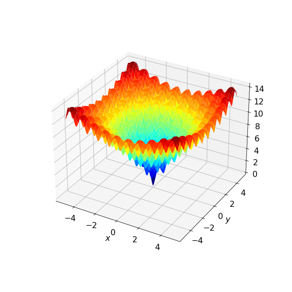
(a) Ackley function

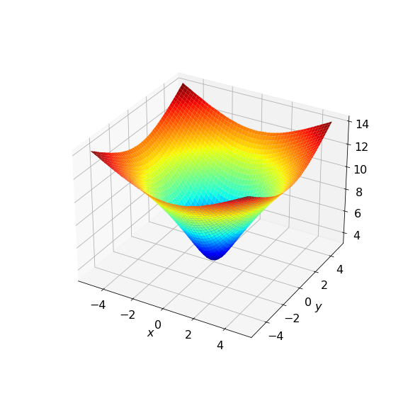
(b) Gaussian smoothed function with parameter $t=1$

Figure 3: Visualization of the Ackley function and its Gaussian smoothed function.

We illustrate the optimization results in Table 3 and Figure 4. The GH methods successfully reach near the optimal solution $(0,0)$ when the decreasing speed of $t$ is not so fast, while ZOSGD is stuck in a local minimum in the immediate vicinity of the initial point $(5,5)$. Please note that GradOpt succeeds in optimization without decreasing the smoothing parameter since the optimal solution of the smoothed function with $t=1$ almost matches that of the original target function.

Table 3: Optimization results of the Ackley function. The global optimum is $f(0,0)=0$.

	Methods	$(x,y)$	$f(x,y)$
SGD algo.	ZOSGD	$(4.99,4.99)$	$12.63$
GH algo.	ZOGradOpt $(\gamma=0.5)$	$(4.2\times 10^{-3},1.9\times 10^{-3})$	$\mathbf{1.4\times 10^{-2}}$
	ZOGradOpt $(\gamma=0.8)$	$(-2.2\times 10^{-3},6.7\times 10^{-3})$	$\mathbf{8.1\times 10^{-2}}$
	$\text{ZOSLGH}_{\text{r}}\ (\gamma=0.995)$	$(1.97,1.97)$	$6.56$
	$\text{ZOSLGH}_{\text{r}}\ (\gamma=0.999)$	$(-3.6\times 10^{-3},-4.6\times 10^{-3})$	$\mathbf{1.7\times 10^{-2}}$

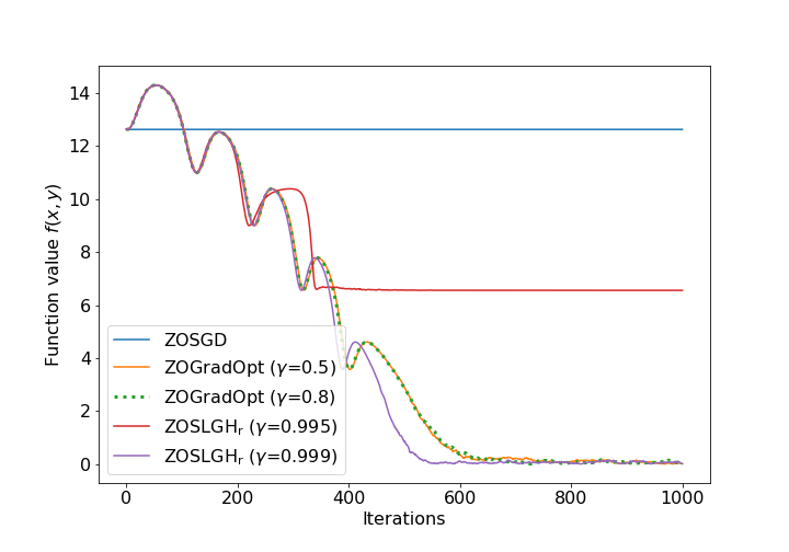
(a) Function value $f(x,y)$ versus iterations.

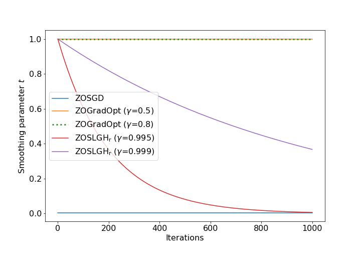
(b) Smoothing parameter $t$ versus iterations.

Figure 4: Plots of the function value and the smoothing parameter during optimization of the Ackley function.

D.2 Rosenbrock Function

Let us define the Rosenbrock function in 2D as

$$f(x,y)=100\left(y-x^{2}\right)^{2}+\left(1-x\right)^{2},$$

whose global optimum is $f(1,1)=0$. This function is difficult to optimize because the global optimum lies inside a flat parabolic shaped valley with low function value (Figure 5(a)). Since this function is polynomial, we can calculate the GH smoothed function analytically (see [Mobahi & Ma (2012)]):

$$F(x,y,t) :=\mathbb{E}_{u_{x},u_{y}}[f(x+tu_{x},y+tu_{y})],\quad\left(u_{x},u_{y}\sim\mathcal{N}(0,1)\right)$$

$$=100x^{4}+(-200y+600t^{2}+1)x^{2}-2x+100y^{2}-200t^{2}y+(300t^{4}+101t^{2}+1).$$

Thus, we applied first-order methods to this function. The stepsize and iteration number were set to $\beta=1\times 10^{-4}$ and $T=20000$, respectively. The initial smoothing parameter for the GH algorithms (GradOpt and $\text{SLGH}_{\text{r}}$) was set to $t_{1}=1.5$, where the smoothed function became almost convex around the optimal solution (Figure 5(b)). We set the initial point for the optimization as $(x,y)=(-3,2)$.

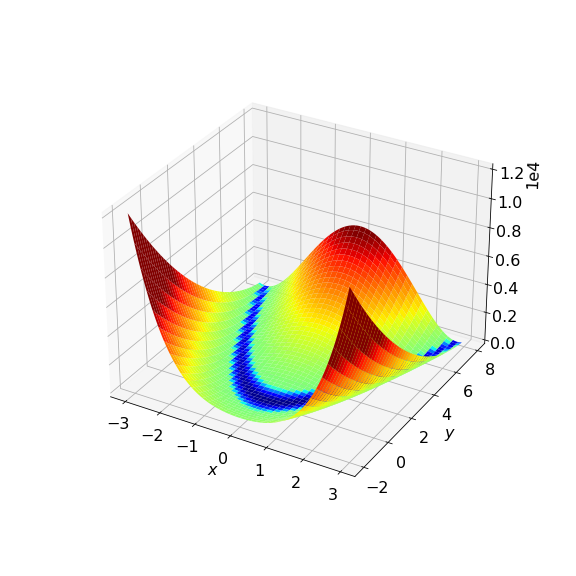
(a) Rosenbrock function

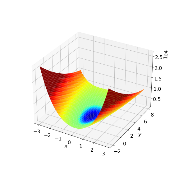
(b) Smoothed function with parameter $t=1.5$

Figure 5: Visualization of the Rosenbrock function and its Gaussian smoothed function.

We illustrate the optimization results in Table 4, Figure 6 and Figure 7. The GH methods can decrease the function value much faster than GD. This is because the smoothed function is much easier to optimize than the original function while its optimal solution is close to that of the original one. In the early stage of optimization, the GH methods reach near a point $(0,2)$, which is a good initial point for optimization, while GD falls into a point in the flat valley, which is far from the optimal solution. (Figure 7).

Table 4: Optimization results of the Rosenbrock function. The global optimum is $f(1,1)=0$.

	Methods	$(x,y)$	$f(x,y)$
GD algo.	GD	$(0.468,0.216)$	$0.284$
GH algo.	GradOpt $(\gamma=0.5)$	$(0.817,0.667)$	$\mathbf{3.36\times 10^{-2}}$
	GradOpt $(\gamma=0.8)$	$(0.808,0.652)$	$\mathbf{3.70\times 10^{-2}}$
	$\text{SLGH}_{\text{r}}\ (\gamma=0.995)$	$(0.819,0.670)$	$\mathbf{3.27\times 10^{-2}}$
	$\text{SLGH}_{\text{r}}\ (\gamma=0.999)$	$(0.795,0.631)$	$\mathbf{4.19\times 10^{-2}}$

(a) Function value $f(x,y)$ versus iterations.

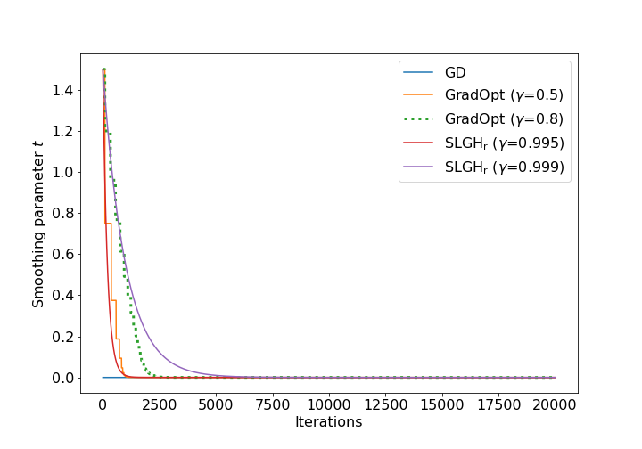
(b) Smoothing parameter $t$ versus iterations.

Figure 6: Plots of the function value and the smoothing parameter during optimization of the Rosenbrock function.

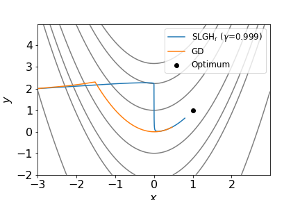
Figure 7:

Comparison of output sequences between GD and $\text{SLGH}_{\text{r}}\ (\gamma=0.999)$ with contours

of the Rosenbrock function.

D.3 Himmelblau Function

The Himmelblau function is defined as

$$f(x,y)=(x^{2}+y-11)^{2}+(x+y^{2}-7)^{2}.$$

It has four minimum points in the vicinity of $(x,y)=(3.000,2.000),(-2.805,3.131),(-3.779,-3.283)$, $(3.584,-1.848)$ and one maximum point in the vicinity of $(x,y)=(-0.271,-0.923)$. It takes the optimal value $0$ at the four points. Since this function is also polynomial, we can calculate the GH smoothed function analytically:

$$F(x,y,t):=\mathbb{E}_{u_{x},u_{y}}[f(x+tu_{x},y+tu_{y})],\quad\left(u_{x},u_{y}\sim\mathcal{N}(0,1)\right)$$

$$=x^{4}+(2y+6t^{2}-21)x^{2}+(2y^{2}+2t^{2}-14)x+y^{4}+(6t^{2}-13)y^{2}+(2t^{2}-22)y+(6t^{4}-34t^{2}+170).$$

Thus, we applied first-order methods to this function. The stepsize and iteration number were set to $\beta=1\times 10^{-4}$ and $T=2000$, respectively. The initial smoothing parameter for GH algorithms was set to $t_{1}=2$, where the smoothed function became almost convex around the optimal solution (Figure 8(b)). We set the initial point for the optimization as $(x,y)=(5,5)$.

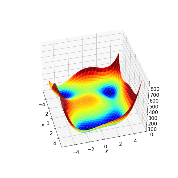
(a) Himmelblau function

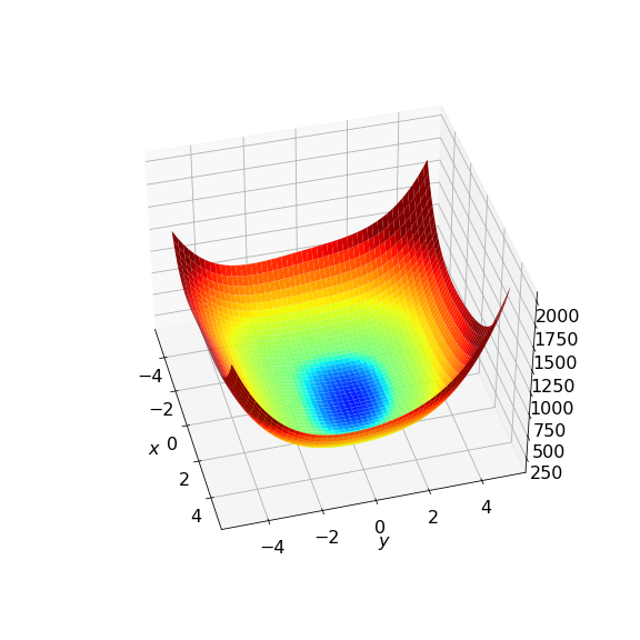
(b) Gaussian smoothed function with parameter $t=2$

Figure 8: Visualization of the Himmelblau function and its Gaussian smoothed function.

Table 5, Figure 9, and Figure 10 show the optimization results. GD and our SLGH algorithms successfully reach near the global optimum, while GradOpt fails to decrease the function value. This is because the optimal solution of the smoothed function when $t=2$ lies near the maximum point of the original Himmelblau function $(-0.271,-0.923)$. Figure 10 describes detailed optimization process. Our SLGH algorithm succeeds in returning to the optimal solution once it has passed by reducing $t$. In contrast, GradOpt reaches the vicinity of a minimum of the smoothed function without knowing the detailed shape of the original function; as a result, it is stuck around a local maximum of the original function.

Table 5: Results of optimization of the Himmelblau function. It has a global optimum $f(3,2)=0$.

	Methods	$(x,y)$	$f(x,y)$
GD algo.	GD	$(2.998,2.003)$	$\mathbf{1.6\times 10^{-4}}$
GH algo.	GradOpt $(\gamma=0.5)$	$(2.575,1.437)$	$14.14$
	GradOpt $(\gamma=0.8)$	$(1.573,0.868)$	$80.51$
	$\text{SLGH}_{\text{r}}\ (\gamma=0.995)$	$(2.999,2.002)$	$\mathbf{6.9\times 10^{-5}}$
	$\text{SLGH}_{\text{r}}\ (\gamma=0.999)$	$(2.983,1.897)$	$\mathbf{0.21}$

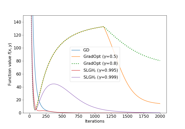
(a) Function value $f(x,y)$ versus iterations.

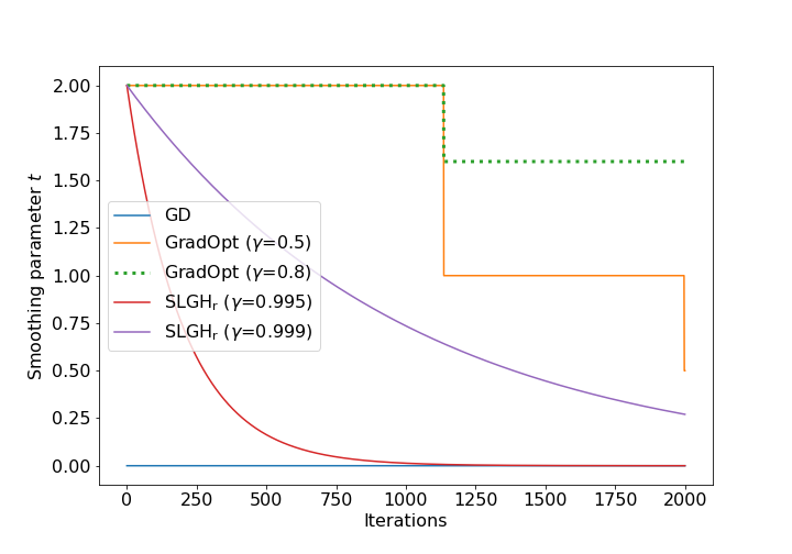
(b) Smoothing parameter $t$ versus iterations.

Figure 9: Plots of the function value and the smoothing parameter during optimization of the Himmelblau function.

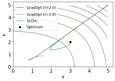
Figure 10: Comparison of output sequences of GradOpt, in which the factor for decreasing the smoothing parameter is $0.8$, and $\text{SLGH}_{\text{r}}\ (\gamma=0.999)$ with contours of the smoothed Himmelblau function. The blue and orange lines represent output sequences of GradOpt when $t=2.0$ and $t=1.6$, respectively.

D.4 Additional Toy Example

At the end of this section, let us present a toy example problem in which $\text{SLGH}_{\text{d}}$, which utilizes the derivative $\frac{\partial F}{\partial t}$ for the update of $t$, outperforms $\text{SLGH}_{\text{d}}$. Let us consider the following artificial non-convex function:

$$f(x,y)=\left\{\begin{array}[]{cc}x^{2}-150\times 1.1^{-((x-10)^{2}+y^{2})}&(x\geq 0)\\ x^{2}/50-150\times 1.1^{-((x-10)^{2}+y^{2})}&(x<0)\\ \end{array}\right..$$

The second term creates a hole around $(x,y)=(10,0)$ (see Figure12(a)), and this function has an optimum in the vicinity of $f(9.319,0)\simeq-56.670$. This function is difficult to optimize for GH methods since the hole around the optimum disappears when the smoothing parameter $t$ is large (Figure12(b)).

We ran $\text{SLGH}_{\text{r}}\ (\gamma=0.995\text{ or }0.999)$ and $\text{SLGH}_{\text{d}}\ (\gamma=0.999)$ with the stepsize (for $x$) $\beta=0.01$ for $T=1000$ iterations. The initial point and initial smoothing parameter were set to $(x,y)=(15,0)$ and $t_{1}=5$, respectively. We set the stepsize for $t$ as $0.01$.

Table 6 and Figure 11 show the optimization results. We can see that only $\text{SLGH}_{\text{d}}$ can decrease $t$ around the hole adaptively, and thus successfully can find the optimal solution.

Table 6: Optimization results of the artificial non-convex function. It has a global optimum in the vicinity of $f(9.319,0)\simeq-56.670$.

	Methods	$(x,y)$	$f(x,y)$
GH algo.	$\text{SLGH}_{\text{r}}\ (\gamma=0.995)$	$(-0.248,2.38\times 10^{-2})$	$-5.52\times 10^{-3}$
	$\text{SLGH}_{\text{r}}\ (\gamma=0.999)$	$(-2.959,-2.18\times 10^{-3})$	$0.175$
	$\text{SLGH}_{\text{d}}\ (\gamma=0.999)$	$(9.319,8.33\times 10^{-3})$	$\mathbf{-56.670}$

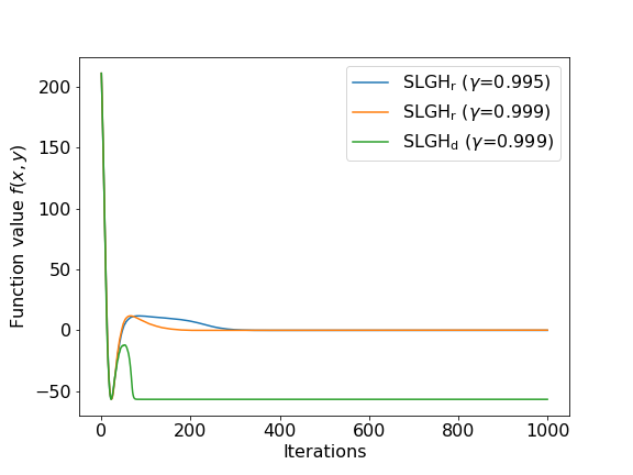
(a) Function value $f(x,y)$ versus iterations.

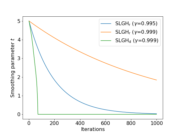
(b) Smoothing parameter $t$ versus iterations.

Figure 11:

Plots of the function value and the smoothing parameter during optimization

of the artificial non-convex function.

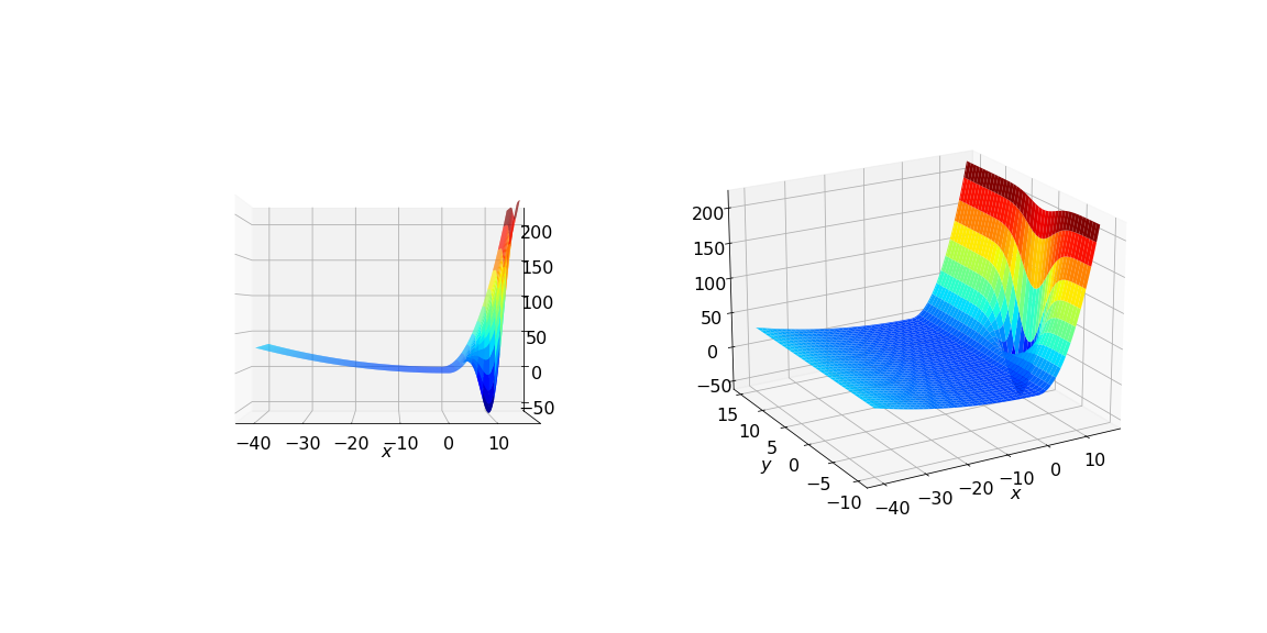
(a) Artificial non-convex function

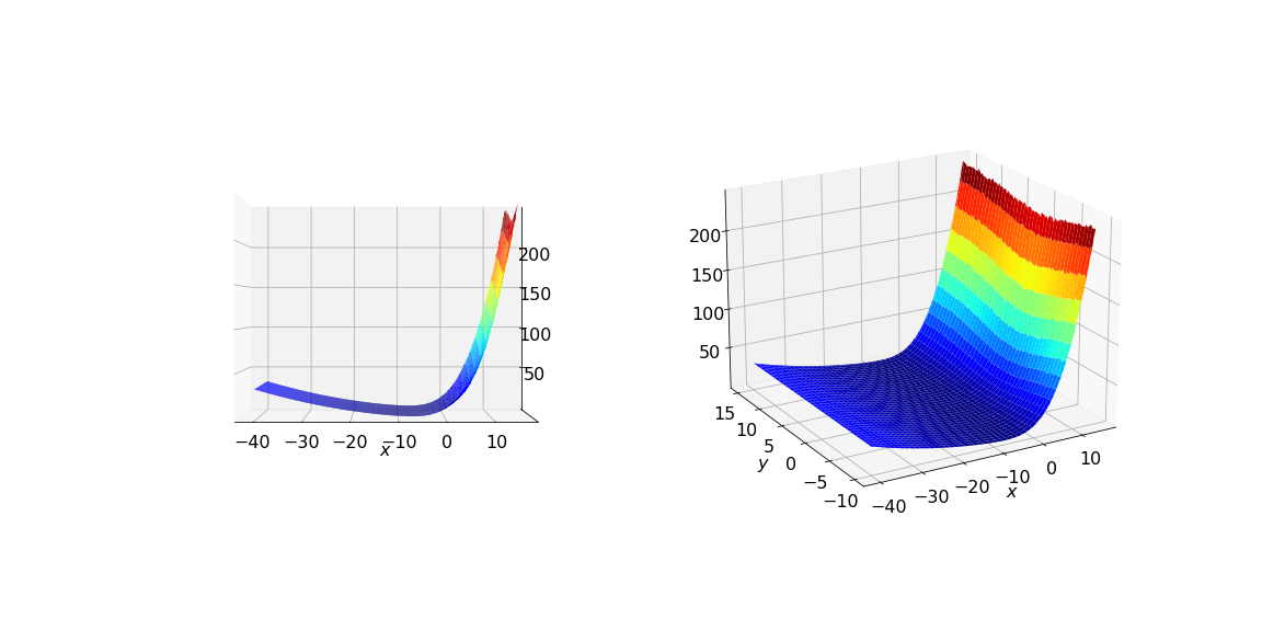
(b) Gaussian smoothed function with parameter $t=5$

Figure 12: Visualization of the artificial non-convex function and its Gaussian smoothed function.

Appendix E Black-box adversarial attack

E.1 Experimental Setup

We used well-trained $\mathop{\rm DNNs}$ for CIFAR10 and MNIST classification tasks as target models, respectively. We adopt the implementation in [Chen et al. (2019)] for ZOSGD and ZOAdaMM. GradOpt [Hazan et al. (2016)] in our implementation adopts the same random gradient-free oracles [Nesterov & Spokoiny (2017)] as with our ZOSLGH methods, rather than their smoothed gradient oracle, where random variables are sampled from the unit sphere. Moreover, we set the stepsize in its inner loop as a constant instead of $\Theta(1/k)$, where $k$ denotes an iteration number in the inner loop, due to less efficiency of the original setting. Therefore, the essential difference between GradOpt and $\text{ZOSLGH}_{\text{r}}$ is whether or not the structure of algorithms is single loop.

As recommended in their work, we set the parameter for ZOAdaMM as ${v}_{0}=10^{-5}$, $\beta_{1}=0.9$, and $\beta_{2}=0.3$. The factor for decreasing the smoothing parameter in ZOGradOpt was set to $0.5$. For all algorithms, we chose the regularization parameter $\lambda$ as $\lambda=10$ and set attack confidence $\kappa=1e-10$. We chose minibatch size as $M=10$ to stabilize estimation of values and gradients of the smoothed function. The initial adversarial perturbation was chosen as $x_{0}=0$, and the initial smoothing parameter $t_{0}$ was $10$ for GH methods and $0.005$ for the others. The decreasing factor for $t$ in the ZOSLGH algorithm was set to $\gamma=0.999$ for both of $\text{ZOSLGH}_{\text{r}}$ and $\text{ZOSLGH}_{\text{d}}$, unless otherwise noted. Other parameter settings are described in Table 7. We used different step sizes for ZOAdaMM because it adaptively penalizes the step size using the information of past gradients [Chen et al. (2019)].

Table 7: Parameter settings in the adversarial attack problems. $T$ represents the iteration number. $\beta$ is the step size for $x$, and $\eta$ is the step size for $t$. $N_{0}$ and $\epsilon_{0}$ are used to determine termination condition of the inner loop in ZOGradOpt: we stop the inner loop and decrease $t$ if the condition $|\frac{1}{M}\sum_{i=1}^{M}f(x_{k+1}+tu_{i})-\frac{1}{M}\sum_{i=1}^{M}f(x_{k}+tu^{\prime}_{i})|\leq\epsilon_{0}$ is satisfied $N_{0}$ times, where $u_{i}$ and $u_{i}^{\prime}\ (i=1,...,M)$ are sampled from $\mathcal{N}(0,\mathrm{I}_{d})$. Each of “3072” and “784” is the dimension of images in CIFAR-10 and MNIST.

	$T$	$\beta$ (other than ZOAdaMM)	$\beta$ (for ZOAdaMM)	$\eta$	$(N_{0},\epsilon_{0})$
CIFAR-10	$10000$	$0.01/3072$	$0.5/3072$	$1\times 10^{-4}/3072$	$(100,5\times 10^{-3})$
MNIST	$20000$	$1/784$	$100/784$	$0.1/784$	$(100,1\times 10^{-3})$

E.2 CIFAR-10

Additional plots

Figures 13 and 14 show additional plots for total loss and $L_{2}$ distortion, respectively. We can see that our ZOSLGH algorithms successfully decrease the total loss value except in cases where images are so difficult to attack that no algorithms succeed in attacking (Figure 13(i), 13(j)). Plots in Figure 14 imply that the algorithms are stuck around a local minimum $x=0$ when they are failed to decrease the loss value.

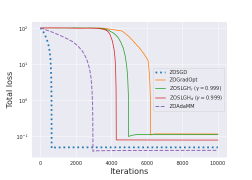
(a) CIFAR-10, Image ID = 1

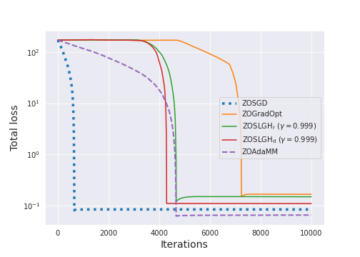
(b) CIFAR-10, Image ID = 16

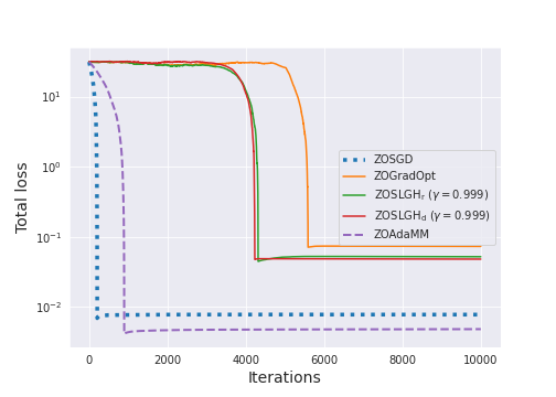
(c) CIFAR-10, Image ID = 37

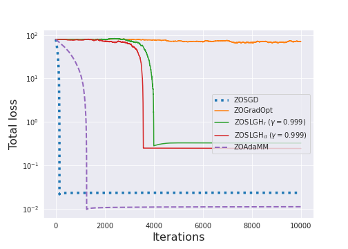
(d) CIFAR-10, Image ID = 7

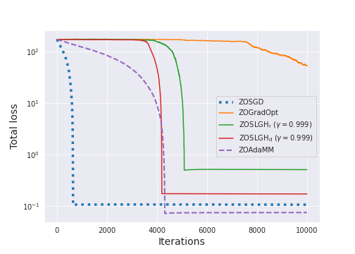
(e) CIFAR-10, Image ID = 51

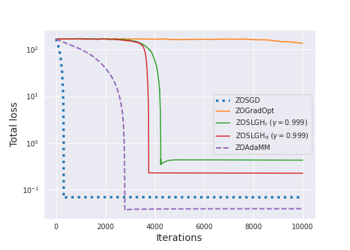
(f) CIFAR-10, Image ID = 96

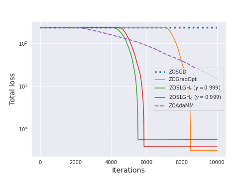
(g) CIFAR-10, Image ID = 39

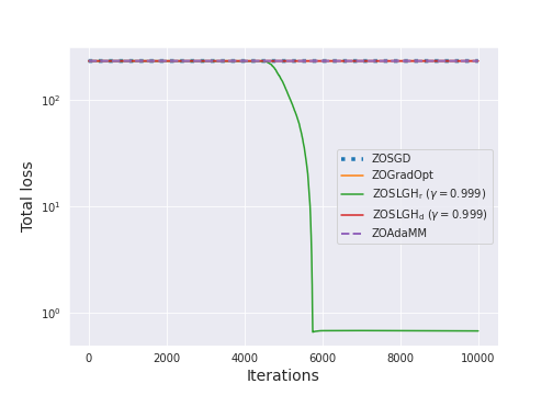
(h) CIFAR-10, Image ID = 104

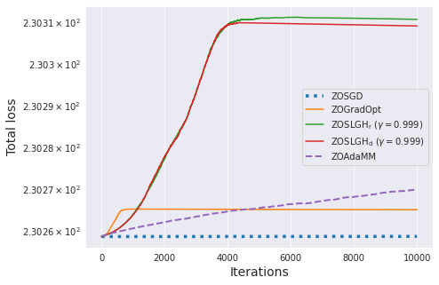
(i) CIFAR-10, Image ID = 14

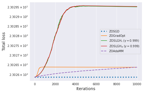
(j) CIFAR-10, Image ID = 41

Figure 13: Additional plots of total loss versus iterations on CIFAR-10 (log scale). (a)-(c) All algorithms can successfully decrease the loss value when images are easy to attack. In particular, in plot (c), SGD-based algorithms can find better solutions than GH-based algorithms. (d)-(f) Only GradOpt fails to attack due to its slow convergence. (g) Only ZOSGD is stuck around a local minimum $x=0$. (h) Only our $\text{ZOSLGH}_{\text{r}}$ algorithm succeeds in escaping the local minimum, and thus it can decrease the loss value more than 200 than other algorithms. (i), (j): These images are so difficult to attack that no algorithms can succeed in attacking.

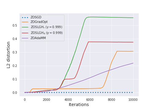
(a) CIFAR-10, Image ID = 39

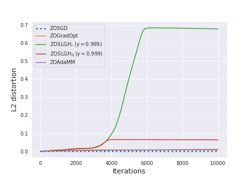
(b) CIFAR-10, Image ID = 104

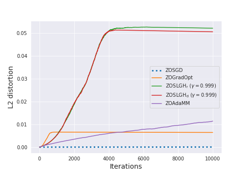
(c) CIFAR-10, Image ID = 14

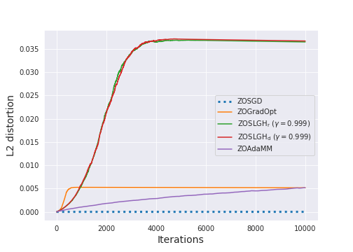
(d) CIFAR-10, Image ID = 41

Figure 14: Plots of $L_{2}$ distortion versus iterations for images that are difficult to attack on CIFAR-10. Each plot of (a)-(d) corresponds to Figure 13(g)-Figure 13(j).

Effect of choice of the parameter $\gamma$ in the ZOSLGH algorithm

We also investigated the effect of choice of the decreasing parameter $\gamma$ in the ZOSLGH algorithm. We compared ZOSGD, $\text{ZOSLGH}_{\text{r}}$ with $\gamma=0.995$, and $\text{ZOSLGH}_{\text{r}}$ with $\gamma=0.999$. All other parameters were set to the same values as before. Figure 15 implies that the decreasing speed of $t$ is associated with a trade-off: a rapid decrease of $t$ yields fast convergence, but reduces the possibility to find better solutions.

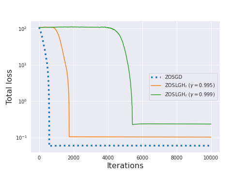
(a) CIFAR-10, Image ID = 8

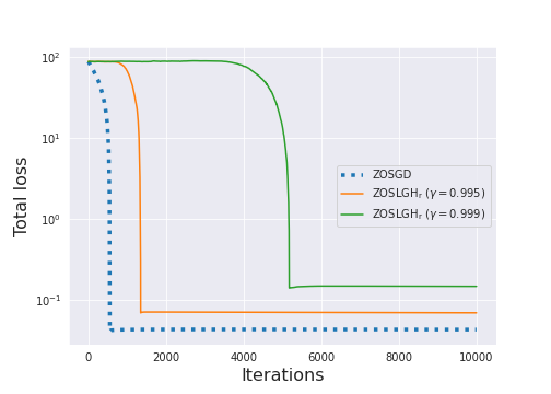
(b) CIFAR-10, Image ID = 66

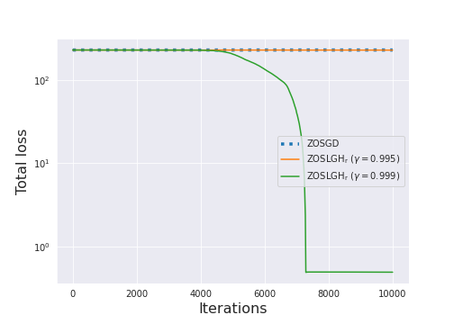
(c) CIFAR-10, Image ID = 105

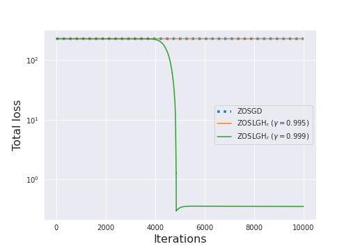
(d) CIFAR-10, Image ID = 89

Figure 15: Comparison of total loss transition of ZOSGD, $\text{ZOSLGH}_{\text{r}}$ with $\gamma=0.995$, and $\text{ZOSLGH}_{\text{r}}$ with $\gamma=0.999$ (log scale).

Generated adversarial examples

Table 8 shows adversarial images generated by different algorithms and their original images.

Table 8: Comparison of adversarial images for CIFAR-10 with different algorithms.

Image ID	39	79	89	115
Original
Classified as	dog	ship	truck	cat
$L_{2}$ distortion:	0	0	0	0
ZOSGD
Classified as	dog (fail.)	airplane	truck (fail.)	horse
$L_{2}$ distortion:	$6.7\times 10^{-5}$	$0.154$	$5.6\times 10^{-5}$	$4.5\times 10^{-3}$
ZOAdaMM
Classified as	dog (fail.)	airplane	truck (fail.)	horse
$L_{2}$ distortion:	$0.226$	$0.145$	$0.131$	$1.6\times 10^{-3}$
ZOGradOpt
Classified as	cat	airplane	truck (fail.)	horse
$L_{2}$ distortion:	$0.304$	$0.254$	$1.1\times 10^{-30}$	$0.192$
$\text{ZOSLGH}_{\text{r}}$
Classified as	cat	airplane	automobile	horse
$L_{2}$ distortion:	$0.540$	$0.212$	$0.282$	$0.076$
$\text{ZOSLGH}_{\text{d}}$
Classified as	cat	airplane	automobile	horse
$L_{2}$ distortion:	$0.359$	$0.174$	$0.241$	$0.075$

E.3 MNIST

Finally, let us show the experimental results on the MNIST dataset. Our ZOSLGH algorithms attain higher success rates than other algorithms on this dataset as well as CIFAR-10 (Table LABEL:table:results_mnist). Moreover, the average number of iterations to achieve the first successful attack becomes comparable to ZOSGD. The main difference from the results on CIFAR-10 is that the average of $L_{2}$ distortion at successful time becomes far larger, from $0.050\sim 0.250$ to $4.25\sim 5.20$. This implies that attacks on MNIST are more difficult than those on CIFAR-10. See Figure 16 and Figure 17 for additional plots for total loss and $L_{2}$ distortion. Figure 10 shows adversarial images generated by different algorithms and their original images.

Table 9: Performance of a per-image attack over $100$ images of MNIST under $T=20000$ iterations. “Succ. rate” indicates the ratio of success attack, “Avg. iters to 1st succ.” is the average number of iterations to reach the first successful attack, “Avg. $L_{2}$ (succ.)” is the average of $L_{2}$ distortion taken among successful attacks, and “Avg. total loss” is the average of total loss $f(x)$ over 100 samples. Please note that the standard deviations are large since the attack difficulty varies considerably from sample to sample.

	Methods	Succ. rate	Avg. iters to 1st succ.	Avg. $L_{2}$ (succ.)	Avg. total loss
SGD algo.	ZOSGD	$67\%$	$1171\pm 1954$	$4.83\pm 4.13$	$73.60\pm 102.70$
	ZOAdaMM	$71\%$	$\textbf{261}\pm 1068$	$\textbf{4.25}\pm 3.36$	$67.49\pm 100.25$
	ZOGradOpt	$84\%$	$6166\pm 4354$	$5.16\pm 2.28$	$28.25\pm 65.35$
GH algo.	$\text{ZOSLGH}_{\text{r}}\ (\gamma=0.999)$	96%	$1537\pm 277$	$\textbf{4.32}\pm 2.44$	$\textbf{11.83}\pm 37.88$
	$\text{ZOSLGH}_{\text{d}}\ (\gamma=0.999)$	96%	$1342\pm 242$	$\textbf{4.37}\pm 2.58$	$\textbf{12.09}\pm 38.56$

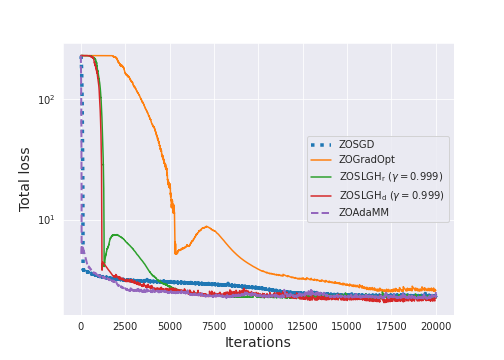
(a) MNIST, Image ID = 7

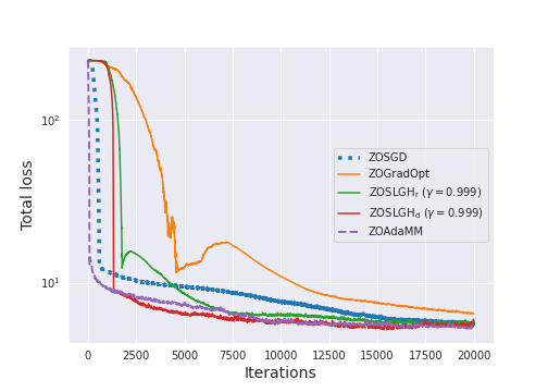
(b) MNIST, Image ID = 58

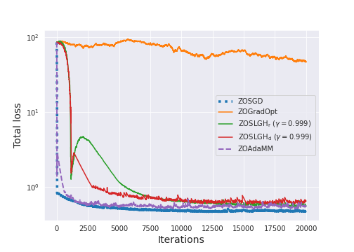
(c) MNIST, Image ID = 18

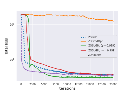
(d) MNIST, Image ID = 94

(e) MNIST, Image ID = 61

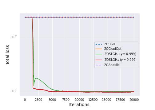
(f) MNIST, Image ID = 30

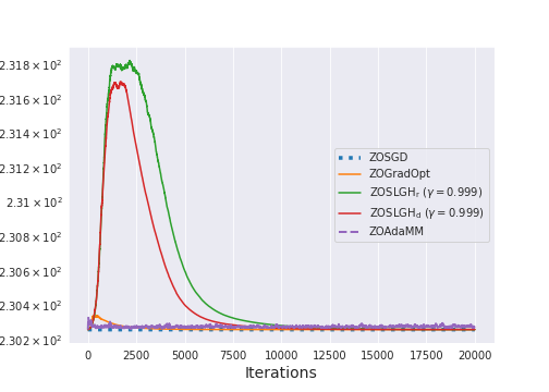
(g) MNIST, Image ID = 68

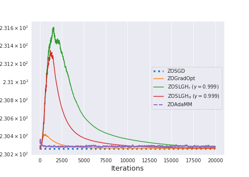
(h) MNIST, Image ID = 82

Figure 16: Additional plots of total loss versus iterations on MNIST (log scale). (a)-(b) All algorithms can successfully decrease the loss value when images are easy to attack. (c)-(d) Only GradOpt fails to attack due to its slow convergence. (e) ZOSGD and ZOAdaMM are stuck around a local minimum $x=0$. (f) Only our ZOSLGH algorithms succeed in escaping the local minimum, and thus they can decrease the loss value more than 200 than other algorithms. (g), (h): These images are so difficult to attack that no algorithms can succeed in attacking.

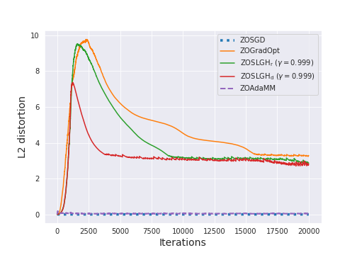
(a) MNIST, Image ID = 61

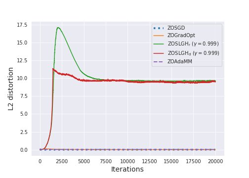
(b) MNIST, Image ID = 30

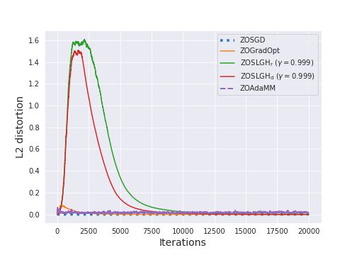
(c) MNIST, Image ID = 68

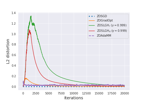
(d) MNIST, Image ID = 82

Figure 17: Plots of $L_{2}$ distortion versus iterations for images that are difficult to attack on MNIST. Each plot of (a)-(d) corresponds to Figure 16(e)-Figure 16(h).

Table 10: Comparison of the adversarial images for MNIST with different algorithms.

Image ID	10	21	48	83
Original
Classified as	0	6	4	7
$L_{2}$ distortion:	0	0	0	0
ZOSGD
Classified as	0 (fail.)	5	9	7 (fail.)
$L_{2}$ distortion:	$4.1\times 10^{-7}$	$1.194$	$1.183$	$1.8\times 10^{-4}$
ZOAdaMM
Classified as	0 (fail.)	5	9	7 (fail.)
$L_{2}$ distortion:	$4.9\times 10^{-14}$	$1.334$	$1.100$	$4.0\times 10^{-14}$
ZOGradOpt
Classified as	2	5	9	9
$L_{2}$ distortion:	$3.898$	$1.378$	$1.903$	$6.379$
$\text{ZOSLGH}_{\text{r}}$
Classified as	2	5	9	9
$L_{2}$ distortion:	$3.867$	$1.261$	$1.106$	$6.075$
$\text{ZOSLGH}_{\text{d}}$
Classified as	2	5	9	9
$L_{2}$ distortion:	$4.048$	$1.222$	$1.059$	$5.722$

References

- Andrei (2008) Andrei, N. An unconstrained optimization test functions collection. Advanced Modeling and Optimization, 10(1):147–161, 2008.
- Aydore et al. (2019) Aydore, S., Zhu, T., and Foster, D. P. Dynamic local regret for non-convex online forecasting. In Advances in Neural Information Processing Systems, pp. 7982–7991, 2019.
- Blake & Zisserman (1987) Blake, A. and Zisserman, A. Visual reconstruction. MIT press, 1987.
- Brox & Malik (2010) Brox, T. and Malik, J. Large displacement optical flow: descriptor matching in variational motion estimation. IEEE transactions on pattern analysis and machine intelligence, 33(3):500–513, 2010.
- C. Zach (2018) C. Zach, G. B. Descending, lifting or smoothing: Secrets of robust cost optimization. In Proc. ECCV, volume 12, pp. 558–574, 2018.
- Carlini & Wagner (2017) Carlini, N. and Wagner, D. Towards evaluating the robustness of neural networks. In 2017 IEEE Symposium on Security and Privacy, pp. 39–57, 2017.
- Chen & Harker (1993) Chen, B. and Harker, P. T. A non-interior-point continuation method for linear complementarity problems. SIAM Journal on Matrix Analysis and Applications, 14(4):1168–1190, 1993.
- Chen (2012) Chen, X. Smoothing methods for nonsmooth, nonconvex minimization. Mathematical programming, 134(1):71–99, 2012.
- Chen et al. (2019) Chen, X., Liu, S., Xu, K., Li, X., Lin, X., Hong, M., and Cox, D. Zo-adamm: Zeroth-order adaptive momentum method for black-box optimization. In Advances in Neural Information Processing Systems, pp. 7204–7215, 2019.
- Cutkosky & Orabona (2019) Cutkosky, A. and Orabona, F. Momentum-based variance reduction in non-convex sgd. In Advances in Neural Information Processing Systems, pp. 15236–15245. Curran Associates, Inc., 2019.
- Dinh et al. (2017) Dinh, L., Pascanu, R., Bengio, S., and Bengio, Y. Sharp minima can generalize for deep nets. In Proceedings of the 34th International Conference on Machine Learning, pp. 1019–1028. PMLR, 2017.
- Evans (2010) Evans, L. Partial Differential Equations. American Mathematical Society, 2010.
- Ghadimi & Lan (2013) Ghadimi, S. and Lan, G. Stochastic first-and zeroth-order methods for nonconvex stochastic programming. SIAM Journal on Optimization, 23(4):2341–2368, 2013.
- Hazan et al. (2016) Hazan, E., Levy, K. Y., and Shalev-Shwartz, S. On graduated optimization for stochastic non-convex problems. In Proceedings of the 33rd International Conference on Machine Learning, pp. 1833–1841, 2016.
- Hemeda (2012) Hemeda, A. A. Homotopy perturbation method for solving systems of nonlinear coupled equations. Applied Mathematical Sciences, 6(93-96):4787–4800, 2012.
- Jain & Kar (2017) Jain, P. and Kar, P. Non-convex optimization for machine learning. Foundations and Trends in Machine Learning, 10(3–4):142–336, 2017.
- Jin et al. (2018) Jin, C., Liu, L. T., Ge, R., and Jordan, M. I. On the local minima of the empirical risk. In Proceedings of the 32nd International Conference on Neural Information Processing Systems, pp. 4901–4910, 2018.
- Kingma & Ba (2015) Kingma, D. P. and Ba, J. Adam: A method for stochastic optimization. In 3rd International Conference on Learning Representations, 2015.
- Li et al. (2017) Li, H., Xu, Z., Taylor, G., Studer, C., and Goldstein, T. Visualizing the loss landscape of neural nets. In Advances in Neural Information Processing Systems, pp. 6389–6399, 2017.
- Liu et al. (2018) Liu, S., Kailkhura, B., Chen, P. Y., Ting, P. S., Chang, S. Y., and Amini, L. Zeroth-order stochastic variance reduction for nonconvex optimization. In Advances in Neural Information Processing Systems, pp. 3727–3737, 2018.
- Mertikopoulos et al. (2020) Mertikopoulos, P., Hallak, N., Kavis, A., and Cevher, V. On the almost sure convergence of stochastic gradient descent in non-convex problems. In Advances in Neural Information Processing Systems, pp. 1117–1128. Curran Associates, Inc., 2020.
- Mobahi (2016) Mobahi, H. Closed form for some gaussian convolutions. arXiv preprint arXiv:1602.05610, 2016.
- Mobahi & Fisher III (2015a) Mobahi, H. and Fisher III, J. W. On the link between gaussian homotopy continuation and convex envelopes. In Energy Minimization Methods in Computer Vision and Pattern Recognition, pp. 43–56, 2015a.