Abstract

In this paper, we examine the (LRS) Bianchi-type-I cosmological model with holographic dark energy. The exact solutions to the corresponding field equations are obtained by using generalized hybrid expansion law (HEL). The EoS parameter $\omega$ for DE is found to be time dependent and redshift dependent and its exiting range for derived model is agreeing well with the current observations. Here we likewise apply two mathematical diagnostics, the statefinder (r, s) and $\omega_{d}-\omega^{{}^{\prime}}_{d}$ plane to segregate HDE model from the $\Lambda CDM$ model. Here the $\omega_{d}-\omega^{{}^{\prime}}_{d}$ diagnostic trajectories is the good tool to classifying the dynamical DE model. We found that our model lies in both thawing region and freezing region. We have also construct the potential as well as dynamics of the quintessence and tachyon scalar field. Some physical and geometric properties of this model along with the physical acceptability of cosmological solution have been discussed in detail.

Keywords : LRS Bianchi-I HDE models; Statefinders; $\omega_{d}-\omega_{d}^{{}^{\prime}}$ plane; Scalar field DE models
PACS: 98.80.-k

1 Introduction

Motivated by the discovery of “black hole thermodynamics [1, 2] Hooft proposed the well known holographic principle (HP)” [3]. As a advanced form of “Plato’s cave ”, the HP describes that all of the info confined in a bulk of space may be visualized as a hologram, which correlates to a concept positioning on the frontier of that space. Afterward, Susskind [4] suggest the exact string hypothesis thought of the rule. Besides, Maldacena [5] recommended the notable “ AdS/CFT correspondence” in 1997, which is the best acknowledgment of Holographic Principle. Presently it notable that Holographic Principle is normally used to be an essential idea of quantum gravity.

According to the basic concepts of quantum gravitational, we can also investigate the nature of DE, by HDE principle. As per this rule, the ‘degrees of freedom’ in a constrained structure must be finite and not measure with the volume of the system [6]. As we mention above that HP is the essential part of “quantum gravity” and has significant potential to solve several long-lasting problems in different fields. The HP can also be used to solve the DE problem. The HP reveal us that all the physical measures of the universe, like energy density of DE ($\rho_{d}$), can be depicted by certain amounts on the limit of the universe. This indicates that only two physical measures “the diminished Planck mass $M_{p}$ and the cosmological length scale $L$”, can be utilized to develop the expression of $\rho_{d}$. In view of the dimensional analysis, we have

$$\rho_{d}=c_{1}M_{p}^{4}+c_{2}M_{p}^{4}L^{-2}+c_{3}L^{4-}+........$$ (1)

here $c_{1},c_{2},c_{3}$ are constants. Author [7] suggest that the $c_{1}$ expression is not viable with Holographic principle. According to the HP, the local quantum field (LQF) theory should not be a decent characterization for a black hole. Particularly, the traditional estimate $\rho_{d}\approx c_{1}M^{4}_{P}$ the (LQF) this explanation should not include any theory. The LQF theory attains a non-trivial ‘UV cutoff’ $\Lambda$. As a consequence of the QF theory, the vacuum fluctuation calculated is $\rho_{d}\approx c_{1}M_{4}^{p}L^{-2}$. The suggestion of HDE was depend on the concept of (QF) theory, that a short distance cut-off is associated to a long-distance cut-off due to the limit set by the establishment of a black hole [8]-[14].

We compared only second term and neglecting other terms then we get HDE as

$$\rho_{d}=3C^{2}M^{2}_{p}L^{-2}$$ (2)

where $C$ is other constant. In Eq.(1) $c_{1}$ term is not present in this expression. It is important to note that this expression of $\rho_{d}$ is obtained by dimensional analysis and applying HP, rather than adding a DE term to the Lagrangian. Because of this remarkable feature HDE theory distinguished from other DE theories. In the cosmological context Fischler and Susskind [15] suggested a new version of the holographic concept in the cosmological evolution. In the framework of the DE problem, HP provides a relation $\rho=H^{2}$. Granda and Olivers suggested a holographic density of the type $\rho\approx\alpha H^{2}+\beta\dot{H}$ in [16], where $\alpha$ and $\beta$ are constants. They contend that their new DE model describes the universe’s accelerated expansion and it is consistent with current observational findings. Bianchi-type models are the most basic and accurate anisotropic models, completely describing anisotropic effects. Chimento et al. [17] looked at a Universe with an interacting dark sector and a decoupling component that may be used to simulate a radiation term. [18] discusses a model of interacting dark matter and dark energy based on a modified holographic Ricci cutoff in a spatially flat FRW spacetime. In [19], a universe with interacting dark matter, holographic dark energy, and dark radiation is examined for FRW spacetime. FRW universe with interacting dark matter, modified holographic Ricci dark energy, and a decoupled baryonic component was studied by Chimento et al. [20]. Chimento et al. [21] also introduced scalar field models through internal space structure generalization of the quintom cosmological scenario.

In this manner numerous cosmologist have proposed the various aspects of these spatially homogeneous and anisotropic Bianchi-type models in various modified theories [22]-[29]. Zadeh [30] examined the astronomical advancement of THDE in Bianchi type-I model with various IR cut-offs. Author [31, 32, 33] dealt with different anisotropic DE cosmological models . Authors [34, 35] worked on the general class of anisotropic cosmological models in particular theories.

In the literature, anisotropic Bianchi type-I, III, and V DE models with the standard perfect fluid have been also widely researched [36]-[42]. Sarkar and Mahanta [43] developed a HDE cosmological model in Bianchi type-I space time with quintessence. Adhav et al. [44] investigated an homogeneous and anisotropic Bianchi type-I universe field with interacting dark matter and HDE. A similar way Pradhan and Amirhashchi [45] constructed a accelerating DE model and investigated some new precise solutions of Einstein’s field conditions in a spatially and anisotropic Bianchi type-V space-time.

The Bianchi type-I string cosmological model with bulk viscosity was examined by Tiwari and Sonia [46] . Many cosmologists [47, 48, 49] have explored the Bianchi type-I models from a different perspective. Now we can say that Spatially homogeneous and anisotropic cosmological models play an important role in the description of large-scale phenomena in the cosmos. Among the numerous dynamical DE models, the cosmological constant is the most important component but it suffers from ‘cosmic coincidence and fine tuning’ problems. As a result of this explanation, various dynamical DE models have been recommended and they were given as family of ‘scalar field models ( quintessence, k-essence, phantom, ghost, etc.), Chaplygin gas as well as holographic DE (HDE)’ models. The authors [50] concluded that the modified structure scalars play an important role in the dynamics of compact object. The authors [51] investigated the oscillatory behaviour of the anisotropy Bianchi -I spacetime. and emphasized the presence of a residue in the energy density in a late time isotropic universe coming from its past anisotropic behaviour. Renyi HDE correspondence is discussed in higher dimensional Kaluza-Klein cosmology [52].

In this manuscript we have chosen LRS Bianchi types-I (LRSBT-I) homogeneous and isotropic model. This model is very important to study space-times where anisotropy occurs at early stage and isotropy at later stage of the evolution of the universe. We have developed various cosmological parameters to describe the dynamics of universe. These parameters are evaluated in terms of $t$ and redshift $z$. Our work is outlined in the following manner: In Sec. $2$, we formulate the basic field equations for LRSBT-I metric. The solutions and the physical behaviour of the cosmological parameters are discussed in Sec. $3$. In Sect. $4$, we have discussed the state finder diagnosis. In Sec. $5$, we have studied the distinct regions in $\omega_{d}-\omega_{d}^{{}^{\prime}}$ plane. In Sec. $6$, we have constructed the DE scalar field models for tachyon and quintessence. The nature of the deceleration parameter ($q$) is discussed in Sec. $7$. We have concluded the results in the last Sec. $8$.

2 LRS Bianchi type-I universe and Basic Field Equations

In this cosmological model we consider the LRS Bianchi type I metric of the form

$$ds^{2}=-dt^{2}+A(t)^{2}dx^{2}+B(t)^{2}\left(dy^{2}+dz^{2}\right),$$ (3)

where the metric coefficients “$A$ and $B$” are function of $t$ only.

In general relativity, Einstein’s field equation with the cosmological constant:

$$R_{ij}-\frac{1}{2}g_{ij}R+\Lambda g_{ij}=-\left(T_{ij}+\bar{T}_{ij}\right)$$ (4)

The notations have their typical significance. The new HDE for actual interpretation and the energy momentum tensor for matter can be composed as : $T_{ij}=\rho_{m}u_{i}u_{j}$, $\bar{T}_{ij}=(\rho_{d}+p_{d})u_{i}u_{j}+g_{ij}p_{d}$, where $\rho_{m}$ and $\rho_{d}$ address the matter energy density and new HDE density, and $p_{d}$ stands for the HDE pressure. The field equations given by Eq. (4) along with the energy momentum tensors defined above for the LRSBT-I metric of three independent equations:

$$2\frac{\ddot{B}}{B}+\frac{\dot{B}^{2}}{B^{2}}=-p_{d}+\Lambda,$$ (5)

$$\frac{\ddot{A}}{A}+\frac{\ddot{B}}{B}+\frac{\dot{A}\dot{B}}{AB}=-p_{d}+\Lambda,$$ (6)

$$2\frac{\dot{A}\dot{B}}{AB}+\frac{\dot{B}^{2}}{B^{2}}=\rho_{m}+\rho_{d}+\Lambda.$$ (7)

Now, as indicated in Refs. [53, 54], the HDE density with IR cut-off is defined as:

$$\rho_{d}=3M^{2}_{p}(kH^{2}+m\dot{H}),$$ (8)

where $k$ and $m$ are the dimensionless parameters and must satisfy the restrictions imposed by the current observational framework with $M^{2}_{p}=8\pi G=1$. The energy conservation law is determined as $T^{ij}_{;j}=0$, gives $\rho_{m}+\dot{\rho_{d}}+3H(\rho_{m}+\rho_{d}+p_{d})=0$. The energy conservation law for matter and dark energy are, separately expressed as $\dot{\rho_{m}}+3H\rho_{m}=0$ and $\dot{\rho_{d}}+3H(\rho_{d}+p_{d})=0$ respectively. Here, $H$ is the Hubble parameter defined by $H=\frac{\dot{a(t)}}{a(t)}$, where the dot represents a time derivative. The Hubble parameter varies with time, not with space, being the Hubble constant $H_{0}$ is the current value. The relative expansion of the universe is parametrized by a dimensionless scale factor $a$. The Hubble constant ($H_{0}$) is important as it is needed to estimate the size and the age of the Universe. $H$ indicates the rate at which the universe is expanding, from the pre mordial “Big Bang”.

3 Solutions and Physical Behaviour of the Model

Here, we have three equations Eq. (5)- Eq. (7) with five unknown parameters namely A, B, $\rho_{d}$, $\rho_{m}$ and $\Lambda$. For solving these equations, we need two more physical assumption. Our first assumption has to taken in Eq. (8) and the second assumption is the scale factor $a(t)$ which is defined as [55, 56] :

$$a=t^{\alpha}e^{\beta t}$$ (9)

here $\alpha$ and $\beta$ are constant. The scale factor is the fundamental function that characterises the global features of our Universe. For the analysis of various problems, an exact equation for this scale factor as a function of physical and conformal time is desirable [57]. In cosmology, the scale factor is a parameter that represents how the universe’s size is changing in relation to its current size.

This results have a linear relationship between the directional Hubble parameters as $H_{1}=nH_{2}$ where $n$ is positive constant. Here $A=\left(t^{\alpha}e^{\beta t}\right)^{\frac{3n}{(n+2)}}$, $B=\left(t^{\alpha}e^{\beta t}\right)^{\frac{3}{(n+2)}}$, then we obtained $H_{1}=\frac{\dot{A}}{A}=\frac{3n}{(n+2)}\left(\frac{\alpha}{t}+\beta\right)$, $H_{2}=\frac{\dot{B}}{B}=\frac{3}{(n+2)}\left(\frac{\alpha}{t}+\beta\right)$ are the directional Hubble Parameters. The Hubble Parameter is derived as:

$$H=\left(\frac{\alpha}{t}+\beta\right)$$ (10)

By using Eq. (9) we obtained deceleration parameter $q=\frac{\alpha}{(\alpha+\beta t)^{2}}-1$. This defines the relation $\beta=\dfrac{1}{13.8}[\left(\frac{\alpha}{0.27}\right)^{1/2}-\alpha]$, between $\alpha$ and $\beta$, by using $t_{0}=13.8Gry$ $q_{0}=-0.73$, we get the corresponding value of $\beta$ [58, 59] [See Table - 1]. From this table, we observe that $\alpha$ increases with the increase of $\beta$. For $0<\alpha\leq 1$, $\beta$ increases but for $\alpha>1$, $\beta$ starts decreasing. In all figures we have considered the three sets of ($\alpha$, $\beta$) as ($0.25$, $0.0516$), ($0.50$, $0.0624$) and ($0.75$, $0.0665$) respectively. It is worth mentioned that for $0<\alpha<1$, our models show the transitioning scenario whereas for $\alpha\geq 1$, the models are in accelerating phase only.

Using Eq. (9) in (8), we obtain the HDE of the model as:

$$\rho_{d}=\frac{3\left(k(\alpha+\beta t)^{2}-\alpha m\right)}{t^{2}}.$$ (11)

By using Eqs. (10)-(11) in energy conservation law $\dot{\rho_{d}}+3H(1+\omega_{d})\rho_{d}=0$, we get the EoS parameter for the model as:

$$\omega_{d}=-\frac{2\alpha(m-k(\alpha+\beta t))}{3(\alpha+\beta t)\left(k(\alpha+\beta t)^{2}-\alpha m\right)}-1.$$ (12)

Solving Eqs. (5)-(7) and using Eqs. (9)-(11), the expressions for different cosmological parameters, $p_{d}$, $\rho_{m}$ and $\Lambda$ are obtained as

$$p_{d}=\frac{3\left(k(\alpha+\beta t)^{2}-\alpha m\right)}{t^{2}}\left(-\frac{2\alpha(m-k(\alpha+\beta t))}{3(\alpha+\beta t)\left(k(\alpha+\beta t)^{2}-\alpha m\right)}-1\right),$$ (13)

$$\rho_{m}=\frac{2}{t^{2}}\left(\frac{\alpha(-k)(n+2)^{2}+9\alpha^{2}(n-1)+9\beta^{2}(n-1)t^{2}+3\alpha(6\beta nt+n-6\beta t+2)}{(n+2)^{2}}+\frac{\alpha m}{\alpha+\beta t}\right),$$ (14)

$$\Lambda=\frac{1}{t^{2}}\left(2\alpha k+3\left(\alpha m-k(\alpha+\beta t)^{2}\right)-\frac{2\alpha m}{\alpha+\beta t}-\frac{6\alpha}{n+2}+\frac{27(\alpha+\beta t)^{2}}{(n+2)^{2}}\right).$$ (15)

The matter density parameter $\Omega_{m}$ and HDE density parameter $\Omega_{d}$ are given by $\Omega_{m}=\frac{\rho_{m}}{3H^{2}}$ and $\Omega_{d}=\frac{\rho_{d}}{3H^{2}}$.

$$\Omega_{m}=\frac{\alpha(-k)(n+2)^{2}+18\alpha^{2}(n-1)+18\beta^{2}(n-1)t^{2}+6\alpha(6\beta nt+n-6\beta t+2)}{3(2\alpha+\beta t)^{2}(n+2)^{2}}+\frac{2\alpha m}{3(\alpha+\beta t)^{3}}$$ (16)

$$\Omega_{d}=k-\frac{\alpha m}{(\alpha+\beta t)^{2}}$$ (17)

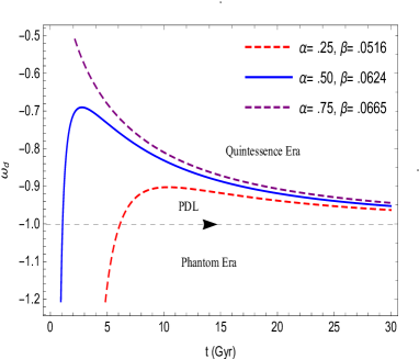
(a) (b) .

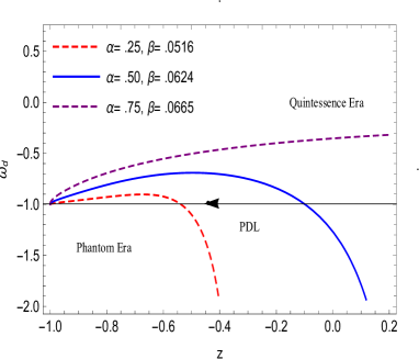
Figure 1: Variation of EoS parameter $\omega_{d}$ versus $t$ and $z$

The redshift of a comoving cosmological source will change with time along the expansion of the universe. The monitoring of the redshift was first proposed by Sandage in 1962 [60], as a useful tool for testing of the cosmology. The expansion of universe can be directly measured by the redshift drift. Therefore, redshift is projected as a valuable addition to other DE probes [61, 62, 63]. Now in our derived model, we use Hubble horizon as a IR cut-off, where $L=H^{-1}$. In general, the transformation between scale factor and redshift is given by $a=\frac{a_{0}}{(1+z)}$, where $a_{0}$ is the present value of $a$. The redshift transformations are useful in validation of models with observational data. Here we obtained cosmological parameters in terms of $t$ as well as redshift in this paper.

The evolution of EoS parameter $\omega_{d}$ versus $t$ and $z$ for different values of $\alpha$ and $\beta$ are shown in fig.1(a)$\&$ 1(b). The EoS parameter exists in both quintessence and phantom regions and also crosses the phantom divided line (PDL) ($\omega_{d}=-1$). Also, the latest cosmological data from SNIa (Supernova Legacy Survey, Gold Sample of Hubble Space Telescope) [64, 65], CMB (WMAP, BOOMERANG) [66] and large scale structure (SDSS) [67] rule out that $\omega_{d}=-1$, they moderately support dynamically developing DE crossing the PDL (see [68, 69, 70]). In cosmology, a redshift is an increase in the wavelength of electromagnetic radiation, with a corresponding fall in frequency and photon energy (such as light). Negative redshift, or blueshift, is the total opposite of positive redshift, with a reduction in wavelength and concomitant rise in frequency and energy. In our LRS Bianchi type-I model, $\omega_{d}=-1$, in late time as $z\to-1$ which suggests that matter in the Universe behaves like a perfect fluid initially. Later on the model is similar to a dark energy model and behaves like a quintessence model and finally approaches -1 then entering the phantom region.

As a consequence, our DE model agrees well with both well-established simulated predictions and current findings.The dynamical features of the model with HEL is most general and interesting feature as obtained from the power law or the exponential expansion. Fig.1(b), shows that the EoS parameter approaches towards $\Lambda$CDM ($\omega_{d}=-1$) in late time.

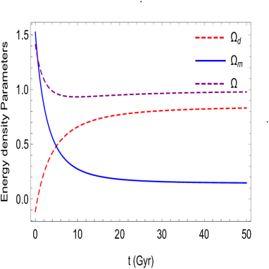
(a) (b) ‘

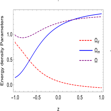
Figure 2: Variation of energy density parameters.

Figure 2 describe the behaviour of energy density parameters with respect to time and redshift $z$ respectively. In the late time the total energy density $\Omega\to 1$ of the universe approaches to unity at low redshift region as clearly shown in Figure 2(a) $\&$ 2(b).

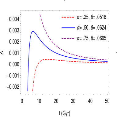
(a) (b)

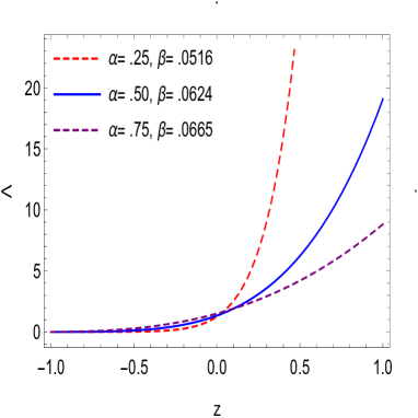
Figure 3: Variation of cosmological constant $(\Lambda)$.

Figures $3a$ $\&$ $3b$ depict the behavior of the ‘cosmological constant $\Lambda$’ versus $t$ and redshift $z$ respectively and show the universe’s expanding mode. We observed that the cosmological parameter is the positive decreasing function of time and redshift $(z\to-1$) and approaches towards zero in late time. Which is a good agreement with recent SNe Ia observation [71, 72]. Authors [73, 74, 75] propose the existence of a positive cosmological constant with a magnitude of $\Lambda(Gh/c3)\approx 10^{-123}$. The most impressive clarification for these info is that the dark energy compares to a positive cosmological constant. These findings on the amplitude and redshift of type Ia supernovas show that our universe is accelerating, with cosmological density produced by the cosmological expansion. The outcome suggests a very minute positive value having magnitude $10^{-123}$.

4 Statefinder

The Statefinder is a geometrical diagnostic and allows us to characterize the properties of dark energy in a model independent manner. The Statefinder is dimensionless and is constructed from the scale factor of the Universe and its time derivatives only. In our model we demonstrate that the Statefinder diagnostic can effectively differentiate between different forms of dark energy.

The stability of DE models can also be examined through the statefinder diagnostic pair $(r,s)$, which gives us an idea related to the dynamical nature of the model. The statefinder parameters $(r,s)$ [76, 77, 78] are a pair of parameters that explore the dynamics of the universe’s expansion by using the higher derivatives of the scale factor. In fact, the trajectories in the $(r,s)$ plane corresponding to different cosmological models show qualitative behaviour.

$$r=\frac{\dddot{a}}{aH^{3}}=\frac{\alpha(-3\alpha-3\beta t+2)}{(\alpha+\beta t)^{3}}+1$$ (18)

$$s=\frac{r-1}{3(-\frac{1}{2}+q)}=\frac{\alpha(-3\alpha-3\beta t+2)}{3(\alpha+\beta t)^{3}\left(\frac{1}{2}-\frac{\alpha}{(\alpha+\beta t)^{2}}\right)}$$ (19)

In the derived model, the ($r,s$) trajectories divide the region into two parts for the various value of the $\alpha$ and $\beta$ as shown in figure 4a. The region $r<1$ ,$s>0$ shows the quintessence era and $r>1$ ,$s<0$ shows the Chaplygin Gas (CG)region. The region $r=1$ ,$s=2/3$ describing the HDE and region $r=1$ ,$s=0$ approaches to $\Lambda$CDM model. In figure 4b, the trajectories $(r,q)$ show the evolution of the universe. Our model starts with SCDM ($(r,q)=(1,0.5)$), $\Lambda$CDM ($(r,q)=(1,0)$) and tends to SS ($(r,q)=(1,-1)$) model as shown in figure by the dots.

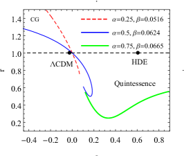
(a) (b)

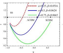
Figure 4: Plots of $r$ versus $s$ and $r$ versus $q$ .

5 $\omega_{d}-\omega_{d}^{{}^{\prime}}$ plane

The EoS parameter of dark energy $\omega_{d}=p_{d}/\rho_{d}$, plays a key role in observational cosmology. According to the distinct region in the $\omega_{d}-\omega^{\prime}_{d}$ plane, Caldwell and Linder [79, 80] categorized the quintessence models defined by the quantities $\omega_{d}$ and $\omega^{\prime}_{d}$ and divide into two parts ”thawing” and ”freezing,” region. Some researchers have recently examined the evolution of quintessence DE models on the $\omega_{d}-\omega^{\prime}_{d}$ plane, where $\omega^{\prime}_{d}$ is the time derivative of $\omega_{d}$ with respect to $\log a$.

$$\omega^{\prime}_{d}=\frac{d\omega_{d}}{d\log a}=\frac{\alpha t\left(3\alpha^{2}k^{2}-3km(\alpha-\beta t)(\alpha+\beta t)-2\beta m^{2}(\alpha+\beta t)^{2}\right)}{3(\alpha+\beta t)^{3}(\alpha k-m(\alpha+\beta t))^{2}}$$ (20)

In our derived model the quintessence region asymptotically approaches to zero. Later this analysis was extended by many researchers to other dynamic DE models. Clearly, a fixed point at (-1,0) is the $\Lambda$ CDM in the $\omega_{d}-\omega^{\prime}_{d}$ plane.

Finally we analyzed the evolutionary behavior of the EoS parameter of the HDE in figure $5$. The trajectories lies in both freezing and thawing regions for three values of parameters $\alpha$ and $\beta$ as clearly shown in figure.

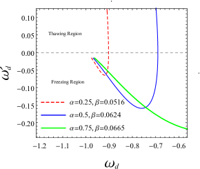
Figure 5: Plot of $\omega_{d}-\omega^{\prime}_{d}$.

6 Scalar Field DE Models

6.1 Tachyon scalar field model of HDE

To depicts the accelerated expansion and evaluation of universe, the tachyon field (TF) is one of the DE candidates [81, 82]. Some tachyon condensate by an powerful Lagrangian density [83, 84] recommends a tachyon field is given by

$$L=-V(\phi)\sqrt{1+\partial_{i}\phi\ \partial^{i}\phi}$$ (21)

Tachyon is observed the most important DE constituent which explain the accelerated expansion of the universe. The EoS parameter of the tachyon DE matter distribution lies between $-1$ and $0$ [85]. The ‘energy density $\rho_{d}$’ and ‘pressure $p_{d}$’ associated with Scalar field ($\phi$) and ‘scalar potential $V(\phi)$’ for tachyon matter distribution are read as:

$$p_{d}=\left(1-\dot{\phi}^{2}\right)^{1/2}V(\phi)$$ (22)

$$\rho_{d}=\frac{V(\phi)}{\sqrt{1-\dot{\phi}^{2}}}$$ (23)

Here, $\dot{\phi}^{2}$ is the scalar field and $V(\phi)$ is the potential respectively.
From Eqs. (22) - (23) and using Eqs. (11) and (13), the scalar $\phi$ and potential $V(\phi)$ are determined as:

$$\phi=\int\sqrt{\frac{2}{3}}\sqrt{-\frac{\alpha(m-k(\alpha+\beta t))}{(\alpha+\beta t)\left(k(\alpha+\beta t)^{2}-\alpha m\right)}}\,dt+c_{1}$$ (24)

$$V(\phi)=\sqrt{3}\sqrt{\frac{\left(k(\alpha+\beta t)^{2}-\alpha m\right)\left(-2\alpha k+3\left(k(\alpha+\beta t)^{2}-\alpha m\right)+\frac{2\alpha m}{\alpha+\beta t}\right)}{t^{4}}}$$ (25)

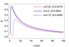
(a) (b)

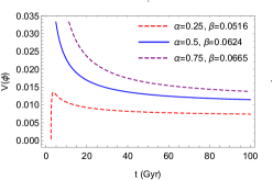
Figure 6: Plots of $\dot{\phi}$ and $V(\phi)$ for tachyon field .

We likewise present an extensive examination of the cosmological results of homogeneous tachyon matter coinciding with non-relativistic matter and radiation, with an emphasis on the converse square and exponential potentials for the tachyonic scalar field. Figures $6a$ and $6b$ show that the scalar field $\phi$ and potential $V(\phi)$ both remains positive as time advances in our determined model. The dynamical behaviour of the tachyon field associated with an exponential potential is presented, and we demonstrate that the pre-inflation dynamics in modified loop cosmology and standard loop quantum cosmology are remarkably similar.

6.2 Quintessence scalar field model of HDE

Quintessence is a conceptual formulation of DE characterized by homogeneous variable ‘Scalar field and the potential’, which are essential for the expansion of the universe [86]. For the quintessence scalar $\phi$, the general formulation of action is as follows:

$$S=\int{d^{4}x\sqrt{-g}\left(-V(\phi)-\frac{1}{2}g^{ij}\partial_{i}\phi\partial_{j}\phi\right)}$$ (26)

The EoS parameter in the quintessence model indicates that the accelerated expansion of the universe exists for $-1\leq\omega\leq-\frac{1}{3}$ [83]. For the quintessence model, the relations of $\rho_{d}$ and $p_{d}$ in the form of ‘$\phi$’ and ‘$V(\phi)$’ are established as [69]:

$$p_{d}=\frac{1}{2}\left(\dot{\phi}^{2}-2V(\phi)\right)$$ (27)

$$\rho_{d}=\frac{1}{2}\left(\dot{\phi}^{2}+2V(\phi)\right)$$ (28)

From Eqs. (11), (13), (27) and (28), the scalar $\phi$ and potential $V(\phi)$ for the ‘quintessence model’ are obtained as

$$\phi=\int\sqrt{\frac{3\left(-\frac{2\alpha(m-k(\alpha+\beta t))}{3(\alpha+\beta t)\left(k(\alpha+\beta t)^{2}-\alpha m\right)}-1\right)\left(k(\alpha+\beta t)^{2}-\alpha m\right)}{t^{2}}+\frac{3\left(k(\alpha+\beta t)^{2}-\alpha m\right)}{t^{2}}}\,dt+c_{2}$$ (29)

$$V(\phi)=\frac{k\left(3\alpha^{3}+3\beta^{3}t^{3}+\alpha^{2}(9\beta t-1)+\alpha\beta t(9\beta t-1)\right)+\alpha m(-3\alpha-3\beta t+1)}{t^{2}(\alpha+\beta t)}$$ (30)

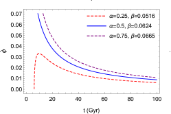
(a) (b)

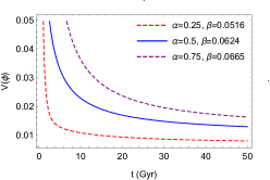
Figure 7: Plots of $\dot{\phi}$ and $V(\phi)$ for quintessence field .

Figures $7a$ and $7b$ depict the growth of the ‘scalar field $\phi$’ and ‘ potential $V(\phi)$’ with time $t$ for all three values of $\alpha$ and $\beta$ in our derived model. The Scale field and potential diminish with time and tends to be low positive at the present epoch.

7 Deceleration parameter for the Model

From the Table-1, we observe that $\alpha$ increases with the increase of $\beta$. For $0<\alpha\leq 1$, $\beta$ increases but for $\alpha>1$, $\beta$ starts decreasing. It is worth mentioned that for $0<\alpha<1$, our models show the transitioning scenario whereas for $\alpha\geq 1$, the models are in accelerating phase only.

Figure $8(a)$ depicts the variation of DP ($q$) with time $t$. Because DP ($q$) lies between the range $-1<q<0$, SNe Ia data reveals the expansion of the present universe in accelerating mode. As a result, the value of the decelerating parameter matches recent data.

We have demonstrated in Fig. $8(b)$ that expansion of $q(z)$ takes place with the change of signature flipping from a decelerating to an accelerating phase. We also observed that $q$ tends to $-1$ as $z$ approaches to $-1$. SNe Ia data shows the progression from previous deceleration to current acceleration. The transition point $z_{t}=0.46\pm 0.13$ at $(1\;\sigma)$ c.l. was investigated in 2004 by the HZSNS group [74]. In 2007, this value of $z_{t}$ was improved by $z_{t}=0.43\pm 0.07$ at $(1\;\sigma)$ c.l. [87]. SNLS first year data set [88] combined with ESSENCE supernova data [89], provide a progress redshift $z_{t}\sim 0.6(1\;\sigma)$ in improved agreement with the flat $\Lambda$CDM model ($z_{t}=(2\Omega_{d}/\Omega_{m})^{\frac{1}{3}}-1\sim 0.66$).

Again $q(z)$ is reconstructed by the joined $(SNIa+CC+H_{0})$, and obtained the transition redshift $z_{t}={0.69}^{+0.09}_{-0.06},{0.65}^{+0.10}_{-0.07}$ and ${0.61}^{+0.12}_{-0.08}$ within $(1\sigma)$ [90] and found consistent with past outcomes [91, 92, 93, 94, 95] including the $\Lambda CDM$ expectation $z_{t}\approx 0.7$. $0.6\leq z_{t}\leq 1.18$ ($2\sigma$, joint examination ) [96] is the other limit of transition redshift.

From the figure $8(b)$, the transitioning redshifts occur at $z_{t}\cong 0.6921$ (for $\alpha=0.25$ & $\beta=0.9516$); $z_{t}\cong 0.4443$ (for $\alpha=0.50$ & $\beta=0.0624$), and $z_{t}\cong 0.995$ (for $\alpha=0.75$ & $\beta=0.0665$) for above three cases which are found to be well consistent with the recent 36 observational Hubble data (OHD) provides the redshift range $0.07\leq z\leq 2.36$ [97]. Comprising 740 SNIa with JLA indicates the redshift range ‘$0.01\leq z\leq 1.30$’. Obviously, our results are in good accordance with those reported in Refs. [74, 89, 96, 97].

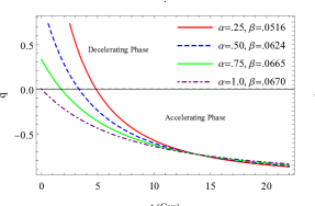
(a) (b)

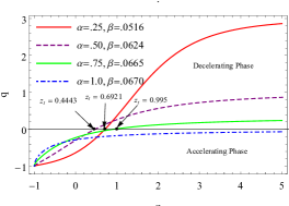
Figure 8: Plots of Deceleration parameter $q$ versus $t$ and redshift $z$.

Table 1: The behaviour of physical parameter

$\alpha$	$\beta$	$q$	$\omega$	$\Omega_{d}$	$\Omega_{m}$	$\Omega$	$r$	$s$	$\omega_{d}^{{}^{\prime}}$
0.25	0.0516124	1.00372	4.93611	-0.115795	2.06244	1.94665	6.33415	3.52981	59.0776
0.5	0.0623788	0.280993	-0.711735	0.232561	0.863276	1.09584	1.25779	-0.392361	0.232003
0.75	0.0664251	-0.0377516	-0.494967	0.386196	0.539123	0.925319	0.293123	0.438168	-0.224348
1.	0.0669928	-0.222349	-0.53636	0.475172	0.400258	0.87543	0.0385825	0.443653	-0.124511
1.25	0.0653375	-0.344267	-0.589897	0.533937	0.326571	0.860507	-0.0173261	0.401661	-0.0699145
1.5	0.0621031	-0.431397	-0.635868	0.575933	0.282205	0.858139	-0.00564742	0.359906	-0.041409
1.75	0.0576721	-0.497056	-0.673521	0.607581	0.253154	0.860735	0.0304176	0.324149	-0.0255545
2.	0.0522939	-0.54846	-0.704391	0.632358	0.232952	0.86531	0.0744813	0.294247	-0.0161907
2.25	0.0461414	-0.589887	-0.729989	0.652325	0.218254	0.87058	0.119843	0.269189	-0.0103853
2.5	0.0393408	-0.624037	-0.751496	0.668786	0.207177	0.875963	0.163705	0.248003	-0.00664547
2.75	0.0319872	-0.65271	-0.769794	0.682606	0.198589	0.881195	0.204962	0.229904	-0.00416254
3.	0.0241546	-0.677148	-0.785542	0.694385	0.191773	0.886159	0.243268	0.214284	-0.00247481

8 Conclusion

In this paper we have developed an anisotropic dark energy cosmological model in the framework of the LRS Bianchi type-I metric. The anisotropic behaviour of the model is simulated by taking HSF scale factor. In this model we are able to get the exact solutions to the field equations by using the hybrid scale factor. This manuscript depends on the HP and dimensional analysis and explored various parameters in the context of HDE, like EoS parameter, density parameter, and cosmological constant. In addition, the state finder trajectories and $\omega_{d}-\omega_{d}{{}^{\prime}}$ plane are also diagnosed. We also analyzed the Hubble parameter for HDE, for both, theoretical and observational aspects.

The main findings of our model are as follows.

• The EoS parameter, which is a function of time and redshift, has been displayed in Figs. $1(a)$ and $1(b)$. Now in our derived model, we have obtained a quintessence and phantom region and crosses the Phantom divided line for three values of ($\alpha$, $\beta$) are shown in Figs. $1(a)$ and $1(b)$. From the graph it is clear that the universe is under the influence of dark energy as the equation of state predicted accelerated expansion phase

• Figs. $2a$ $\&$ $2b$ depict the overall density parameter, which has been matched with $\Lambda CDM$ and approaches to Unity i.e. $\Omega\equiv 1$ for the different values of ($\alpha$, $\beta$).
  

• Figures $3a$ $\&$ $3b$ depict the evolution of the cosmological constant versus $t$ and $z$ respectively. Here $\Lambda$ is a positive decreasing function and approaches towards zero.

• As illustrated in Figs. $4a$ and $4b$, the trajectories of ‘ $(r,s)$ and $(r,q)$’ for various values of $\alpha$ and $\beta$ have been displayed. During the early time, the statefinder trajectory $(r,s)$ plane is separated into two regions: “ $r<1,s>0$ quintessence region and the $r>1,s<0$ Chaplygin Gas”, and its approaches to $\Lambda$CDM $(r,s)=(1,0)$ in the late time. The trajectory $(r,q)$ evolves from the region of (SCDM) in the $(r-q)$ plane and approaches the SS model in late time.

• In Fig. $5$ we have analyzed the evolutionary behaviour of the EoS parameter of the HDE models by constructing the $\omega_{d}-\omega_{d}^{{}^{\prime}}$ plane and found that $\omega_{d}^{{}^{\prime}}<0$ for $\omega_{d}<0$ for the HDE model implying the plane to lie in the freezing region as well as $\omega_{d}^{{}^{\prime}}>0$ for $\omega_{d}<0$ thawing region.

• We have also constructed the potential as well as dynamics of the quintessence and tachyon scalar field see Figs $6$ & $7$.

• Figure $8(b)$ shows the transition redshift from decelerated to accelerated expansion occurs at $z_{t}\cong 0.6921$ (for $\alpha=0.25$ & $\beta=0.9516$); $z_{t}\cong 0.4443$ (for $\alpha=0.50$ & $\beta=0.0624$), and $z_{t}\cong 0.995$ (for $\alpha=0.75$ & $\beta=0.0665$) for above three cases which are in good agreement with those reported in Refs. [74, 89, 96, 97].

As a result, our findings support recent observational data that revealed the current isotropic state. This demonstrates that our model closely matches current observations.

Credit authorship contribution statement

Anirudh Pradhan: Ideas, Formulation and writing- original draft preparation. Vinod Kumar Bhardwaj: Application of mathematical formulation, computation & drawing figures. Archana Dixit: Writing- reviewing, validation & editing. Symala Krishannair: Final draft preparation.

Declaration of competing interest

The authors declare that they have no known competing financial interests or personal relationships that could have appeared to influence the work reported in this paper.

References

- [1] J. D. Bekenstein, Black holes and entropy, Phys. Rev. D 7, (1973) 2333 .
- [2] S. W. Hawking, Particle Creation by Black Holes, Commun. Math. Phys. 43, (1975) 199 .
- [3] G. ’t Hooft, Dimensional Reduction in Quantum Gravity, arXiv:gr-qc/9310026v2 (2009).
- [4] L. Susskind, The world as a hologram, J. Math. Phys. 36, (1995) 6377.
- [5] J. M. Maldacena, The Large N limit of super conformal field theories and supergravity, Int.J. Theor. Phys. 38, (1999) 1113.
- [6] S. Wang, Yi Wang and Miao Li, Holographic Dark Energy, Phys. Rep. 696, (2017) 1.
- [7] A. G. Cohen, D. B. Kaplan and A. E. Nelson, Effective Field Theory, Black Holes, and the cosmological constant, Phys. Rev. Lett. 82, (1999) 4971.
- [8] M. Li, A model of holographic dark energy, Phys. Lett. B 603, (2004) 1.
- [9] E. Elizalde et al., Dark energy: vacuum fluctuations, the effective phantom phase, and holography, Phys. Rev. D 71, (2005) 103504.
- [10] E. Elizalde et al., Unifying inflation with dark energy in modified F(R) Horava-Lifshitz gravity, Eur. Phys. J. C 70, (2010) 351.
- [11] K. Bamba, S. Capozziello, S. Nojiri and S. D Odintsov, Dark energy cosmology: the equivalent description via different theoretical models and cosmography tests, Astrophys Space Sci. 342, (2012) 155.
- [12] S. Nojiri and S. D. Odintsov, Unifying phantom inflation with late-time acceleration: scalar phantom–non-phantom transition model and generalized holographic dark energy, Gen. Relativ. Gravit. 38, 1285 (2006) 1285.
- [13] S. Nojiri and S. D. Odintsov, Modified gravity consistent with realistic cosmology: From a matter dominated epoch to a dark energy universe, Phys. Rev. D 74, (2006) 086005.
- [14] M. Jamil, M. U. Farooq and M. A Rashid, Generalized holographic dark energy model, Eur. Phys. J. C 61, (2009) 471.
- [15] W. Fischler and L. Susskind, Holography and cosmology, arXiv preprint hep-th/9806039 (1998).
- [16] L. N. Granda and A. Oliveros, Infrared cut-off proposal for the holographic density, Phys. Lett. B 669 , (2008) 275.
- [17] L. P. Chimento and M. G. Richarte, Interacting dark matter and modified holographic Ricci dark energy plus a noninteracting cosmic component, Phys. Rev. D 85, (2012) 127301.
- [18] L. P. Chimento and M. G. Richarte, Interacting dark matter and modified holographic Ricci dark energy induce a relaxed Chaplygin gas, Phys. Rev. D 84, (2011) 123507.
- [19] L. P. Chimento and M. G. Richarte, Dark radiation and dark matter coupled to holographic Ricci dark energy, The Euro. Phys. J. C 73, (2013) 2352.
- [20] L. P. Chimento, M. Forte and M. G. Richarte, Modified holographic Ricci dark energy coupled to interacting dark matter and non-interacting baryonic, Euro. Phys. J. C 73, (2013) 2285.
- [21] L. P. Chimento, M. Forte and M. G. Richarte, Interal space structure generalization of the quintom, Phys. Rev. D 79, (2009) 043502.
- [22] O. Akarsu and C. B. Kilinc, de Sitter expansion with anisotropic fluid in Bianchi type-I space-time, Astrophys. Space Sci. 326, (2010) 315.
- [23] C. R Mahanta and N. Sarma, Anisotropic ghost dark energy cosmological model with hybrid expansion law, New Astron. 57, (2017) 70.
- [24] A. K Yadav and B. Saha, LRS Bianchi-I anisotropic cosmological model with dominance of dark energy, Astrophys. Space Sci. 337, (2012) 759.
- [25] D. D Pawar, G. G Bhuttampalle and P. K Agrawal, Kaluza–Klein string cosmological model in theory of gravity, New Astron. 65, (2018) 1.
- [26] V. K. Bhardwaj and Archana Dixit, LRS Bianchi type-I bouncing cosmological models in f(R, T) gravity, Int. J Geom. Meth. Mod. Phys. 17, (2020) 2050203.
- [27] G. K. Goswami, M. Mishra, A. K. Yadav and A. Pradhan, Two fluid scenario in Bianchi type-I Universe, Mod. Phys. Lett. A 35, (2020) 2050086.
- [28] A. Pradhan, H. Amirhashchi and R. Jaiswal, A new class of LRS Bianchi type-II dark energy models with variable EoS parameter, Astrophys. Space Sci. 334, (2011) 249.
- [29] R. Chaubey, A. K Sukla and R. Raushan, Locally rotationally symmetric Bianchi type-I cosmological model with dynamical and in f(R) gravity, Pramana- J. Phys. 92, (2019) 1.
- [30] M. A Zadeh, A. Sheykh, H. Moradpour and K. Bamba, Effects of anisotropy on the sign-changeable interacting Tsallis holographic dark energy, Mod. Phys. Lett. A 35, (2020) 2050053.
- [31] B. Saha, Isotropic and anisotropic dark energy models, Phys. Part. Nucl. 45 , (2014) 349.
- [32] R. Chaubey and A. K. Shukla, The anisotropic cosmological models in gravity with , Pramana-J. Phys. 88, (2017) 65.
- [33] A. Pradhan, A. Dixit, S. Singhal, Anisotropic MHRDE model in BD theory of gravitation, Int. J. Geom. Meth. Mod. Phys., 16, (2019) 1950185.
- [34] R. Chaubey and A. K. Shukla, Holographic dark energy model with quintessence in general class of Bianchi cosmological models, Can. J. Phys. 93, (2015) 68.
- [35] R. Chaubey and A. K. Shukla, The general class of Bianchi cosmological models with varying EoS parameter, Astrophys Space Sci. 356, (2015) 181.
- [36] A. Pradhan, A. K. Singh and D. S. Chouhan, Accelerating Bianchi type-V cosmology with perfect fluid and heat flow in Saez-Ballester theory, Int. J. Theor. Phys. 52, 266 (2013) 266.
- [37] J. P. Singh, R. K. Tiwari and P. Shukla, Bianchi Type-III Cosmological Models with Gravitational Constant G and the Cosmological Constant , Chin Phys. Lett. 24, (2007) 3325.
- [38] K. S. Adhav, Statefinder diagnostic for modified Chaplygin gas in Bianchi type- universe, Eur. Phys. J. Plus 126, (2011) 52.
- [39] A. Pradhan, A. Amirhashchi and B. Saha, Bianchi type-I anisotropic dark energy model with constant deceleration parameter, Int. J. Theor. Phys. 50, (2011) 2923.
- [40] A. K. Yadav and L. Yadav, Bianchi type III anisotropic dark energ models with constant deceleration parameter, Int. J Theor. Phys. 50, (2011) 218.
- [41] R. Rakesh, et al., Locally rotationally symmetric Bianchi type-I cosmological model with dynamical and in f (R) gravity, Pramana-J. Phys. 92, (2019) 1.
- [42] A. K. Yadav, A. Pradhan and A. K. Singh, Bulk viscous LRS Bianchi-I universe with and , Astrophys. Space Sci. 337, (2012) 379.
- [43] S. Sarkar and C. R. Mahanta, Holographic dark energy model with quintessence in Bianchi type-I space-time, Int. J. Theor. Phys. 52, (2013) 1482.
- [44] K. S. Adhav, G. B. Tayade and A. S. Bansod, Interacting dark matter and holographic dark energy in an anisotropic universe, Astrophys. Space Sci. 353, (2014) 249.
- [45] A. Pradhan and H. Amirhashchi, Accelerating dark energy models in Bianchi Type-V spacetime, Mod. Phys. Lett. A 26, (2011) 2261.
- [46] R. K. Tiwari and S. Sharma, Bianchi Type-I string cosmological Model with bulk viscosity and time-dependent term, Chin. Phys. Lett. 28, (2011) 090401.
- [47] M. F. Shamir, Locally rotationally symmetric Bianchi type I cosmology in f(R, T) gravity, Eur. Phys. J. C 75, (2015) 1.
- [48] M. F. Shamir and Z. Raza,Locally rotationally symmetric Bianchi type I cosmology in f (R) gravity, Can. J. Phys. 93, (2015) 37.
- [49] M. Sharif and R. Saleem, Statefinder Diagnostic for Dark Energy Models in Bianchi I Universe, Int. J. Mod. Phys. D 21, (2012) 1250046.
- [50] Z. Yousaf, M. Z. Bhatti and U. Farwa, Axially symmetric systems and structure scalars in gravity, Ann. Phys. 433, (2021) 168601.
- [51] B. B. Bizarria, G. A. S. Silva, L. G. Gomes and W. O. Clavijo, The oscillatory anisotropy in the spatially flat cosmological models, Ann. Phys. 432, (2021) 168571.
- [52] A. Saha, S. Ghose, A. Chanda and B. C. Paul, Renyi holographic dark energy in higher dimension cosmology, Ann. Phys. 426, (2021) 168403.
- [53] L. N. Granda and A.Oliveros, New infrared cut-off for the holographic scalar fields models of dark energy, Phys. Lett. B 671, (2008) 199.
- [54] C. P. Singh, M. Srivastava, Viscous cosmology in new holographic dark energy model and the cosmic acceleration, Eur. Phys. J. C 78, (2018) 1.
- [55] B. Mishra, S. K. Tripathy and S. Tarai, Cosmological models with a hybrid scale factor in an extended gravity theory, Mod. Phys. Lett. A 33, (2018) 1850052.
- [56] B. Mishra, S. K. Tripathy and R. P. Ray, Bianchi-V string cosmological model with dark energy anisotropy, Astrophys. Space Sci. 363, (2018) 1.
- [57] M. V, Sazhin, O. S. Sazhina and U. Chadayammuri, The scale factor in the Universe with dark energy, arXiv: 1109.2258[astro-ph.CO] (2011).
- [58] J. V. Cunha, Kinematic constraints to the transition redshift from supernovae type Ia union data, Phys. Rev. D 79, (2009) 047301.
- [59] V. K. Bhardwaj, A. Pradhan and A. Dixit, Compatibility between the scalar field models of tachyon, k-essence and quintessence in gravity, New Astron. 83, (2021) 101478.
- [60] A. Sandage, The change of redshift and apparent Luminosity of galaxies due to the deceleration of selected expanding universes, Astrophys. J. 136, (1962) 319.
- [61] A. Balbi and C. Quercellini, The time evolution of cosmological redshift as a test of dark energy, Mon. Not. Roy. Astron. Soc. 382, (2007) 1623.
- [62] J. P. Uzan, C. Clarkson and G. F. R. Ellis, Time drift of cosmological redshifts as a test of the Copernican principle, Phys. Rev. Lett. 100, (2008) 191303.
- [63] D. Jain and S. Jhingan, Constraints on dark energy and modified gravity models by the cosmological redshift drift test, Phys. Lett. B 692, (2010) 219.
- [64] A. Pierre et al., The Supernova Legacy Survey: measurement of, and w from the first year data set, Astron. Astrophys. 447 , (2006) 31. arXiv:astro-ph/0510447.
- [65] E. Komatsu et al., Five-year wilkinson microwave anisotropy probe observations: cosmological interpretation, Astrophys. J. Suppl. Ser. 180, (2009) 330. arXiv:0803.0547 [astro-ph].
- [66] C. J. MacTavish et al. Cosmological parameters from the 2003 flight of BOOMERANG, Astrophys. J. 647, (2006) 799. arXiv:astro-ph/0507503.
- [67] E. Eisenstein,et al., Detection of the baryon acoustic peak in the large-scale correlation function of SDSS luminous red galaxies, Astrophys. J. 633, (2005) 560. arXiv:astro-ph/0501171
- [68] G. B. Zhao, Probing for dynamics of dark energy and curvature of universe with latest cosmological observations, Phys. Lett B 648 , (2007) 8.
- [69] E. J. Coperland, M. Sami and S. Tsujikawa, Dynamics of dark energy, Int. J. Mod. Phys. D 15, (2006) 1753. arXiv:hep-th/0603057.
- [70] H. Wei and R. G. Cai, Interacting vectorlike dark energy, the first and second cosmological coincidence problems, Phys. Rev. D 73, (2006) 083002.
- [71] S. Perlmutter et al. Discovery of a supernova explosion at half the age of the universe, Nature 391, (1998) 51.
- [72] S. Perlmutter et.al., Measurments of and from 42 High-Redshift Supernovae, Astrophys. J. 517, (1999) 565.
- [73] A. G. Riess et al., Observational evidence from supernovae for an accelerating universe and a cosmological constant, Astrophys. J. 116, (1998) 1009.
- [74] A. G. Riess et al., Type Ia supernova discoveries at from the Hubble Space Telescope: Evidence for past deceleration and constraints on dark energy evolution, Astrophys. J. 607, (2004) 665.
- [75] J. Tonry et al., Cosmological results from high-z supernovae, Astrophys. J. 594, (2003) 1.
- [76] V. Sahni et al., Statefinder-a new geometrical diagnostic of dark energy, Jour. Exper. Theor. Phys. Lett. 77, (2003) 201.
- [77] A. Pradhan, A. Dixit and V. K. Bhardwaj, Barrow HDE model for Statefinder diagnostic in FLRW Universe, Int. J. Mod. Phys. A 36, (2021) 2150030.
- [78] V. K. Bhardwaj, A. Dixit and A. Pradhan, Statefinder hierarchy model for the Barrow holographic dark energy, New Astronomy, 88, (2021) 101623.
- [79] R. R. Caldwell and E. V. Linder, Limits of quintessence, Phys. Revi Lett. 95, (2005) 141301.
- [80] E. V. Linder, The dynamics of quintessence, the quintessence of dynamics. Gen. Relat. Gravit. 40, (2008) 329.
- [81] T. Padmanabhan, Accelerated expansion of the universe driven by tachyonic matter, Phys. Rev. D 66 , (2002) 021301.
- [82] L. R. W. Abramo and F. Finelli, Cosmological dynamics of the tachyon with an inverse power-law potential, Phys. Lett. B 575 (2003) 165.
- [83] E. A. Bergshoeff, et al., T-duality and actions for non-BPS D-branes, JHEP 05 (2000) 009.
- [84] A. Sen, Rolling tachyon, JHEP 04, (2002) 048.
- [85] G. W. Gibbons, Cosmological evolution of the rolling tachyon, Phy. Letts. B 537, (2002) 1.
- [86] A. Pasqua, M. Jamil, R. Myrzakulov and B. Majeed, Power-law entropy-corrected Ricci dark energy and dynamics of scalar fields, Phys. Scr. 86, (2012) 045004.
- [87] A. G. Riess et al., New Hubble space telescope discoveries of type Ia supernovae at : narrowing constraints on the early behavior of dark energy, Astrophys. J. 659, (2007) 98.
- [88] P. Astier et al., The supernova legacy survey; measurment of from the first year data set, Astron. Astrophys. 447, (2006) 31.
- [89] T. M. Davis et al., Scrutinizing exotic cosmological models using ESSENCE supernova data combined with other cosmological probes, Astrophysical J. 666, (2007) 716.
- [90] A. A. Mamon, Constraints on a generalized deceleration parameter from cosmic chronometers, Mod. Phys. Lett. A 33, (2018) 1850056.
- [91] R. Nair et al., Cosmokinetics: a joint analysis of standard candles, rulers and cosmic clocks, J. Cosmol. Astropart. Phys. 01, (2012) 018.
- [92] A. A. Mamon and S. Das, A divergence-free parametrization of deceleration parameter for scalar field dark energy, Int. J. Mod. Phys. D. 25, (2016) 1650032.
- [93] O. Farooq and B. Ratra, Hubble parameter measurement constraints on the cosmological deceleration-acceleration transition redshift, Astrophys. J. 766, (2013) L7.
- [94] J. Magana et al., Cosmic slowing down of acceleration for several dark energy parametrizations, J. Cosmol. Astropart. Phys. 10, (2014) 017.
- [95] A. A. Mamon, K. Bamba and S. Das, Constraints on reconstructed dark energy model from SN Ia and BAO/CMB observations, Eur. Phys. J. C 77, (2017) 29.
- [96] J. A. S. Lima, J. F. Jesus, R. C. Santos and M. S. S. Gill, Is the transition redshift a new cosmological number, arXiv: 1205.4688v3[astro-ph.CO] (2012).
- [97] H. Yu, B. Ratra and Fa-Yin Wang, Hubble parameter and Baryon Acoustic Oscillation measurement constraints on the Hubble constant, the deviation from the spatially flat CDM model, the deceleration-acceleration transition redshift, and spatial curvature, Astrophys. J. 856, (2018) 3.