KDSource, a tool for the generation of Monte Carlo particle sources using kernel density estimation

Abstract

Monte Carlo radiation transport simulations have clearly contributed to improve the design of nuclear systems. When performing in-beam or shielding simulations a complexity arises due to the fact that particles must be tracked to regions far from the original source or behind the shielding, often lacking sufficient statistics. Different possibilities to overcome this problem such as using particle lists or generating synthetic sources have already been reported. In this work we present a new approach by using the adaptive multivariate kernel density estimator (KDE) method. This concept was implemented in KDSource, a general tool for modelling, optimizing and sampling KDE sources, which provides a convenient user interface. The basic properties of the method were studied in an analytical problem with a known density distribution. Furthermore, the tool was used in two Monte Carlo simulations that modelled neutron beams, which showed good agreement with experimental results.

1 Introduction

The calculation of radiation beams is a specific topic of the general radiation transport problem. Normally it is decoupled from the source since the nuclear reactions that govern the generation of particles in the source are independent of the specific interactions that take place in the beam path. In the design of experimental nuclear facilities, radiation beams are usually transported far away from the source both to reduce the background signal in the measurements and the radiation dose of the personnel. When trying to evaluate the beam under different operating conditions, it is useful to have a source that can be re-sampled. A possible solution is to capture the particles that are produced in the position of the source by fission, decay or other events, and transport them into the beam [1]. Although this is the most common approach, its application to Monte Carlo simulation requires complex variance reduction techniques (such as specifically generated weight windows using CADIS and FW-CADIS [2]), and has a high computational cost. Another approach is to use particle lists or track files, in which the particles that cross a specific surface are recorded and reused in a downstream simulation [3]. This method is computationally more efficient but it may create artificial hot spots in the final solution due to the discrete nature of the recorded data. To avoid this problem, a third solution is to use a synthetic source, fitting an analytical distribution for each of the source variables (energy, position, direction and time) [4, 5]. Although this solution is simple, it strongly depends on the expertise or knowledge of the user and usually fails to capture implicit (or less evident) correlations between variables [6, 7]. With this in mind we propose the use of the adaptive multivariate Kernel Density Estimation (KDE) method to estimate the source distribution at a given point in the beam trajectory, which seeks to overcome the discussed limitations of the previous approaches. Similar ideas have been proposed by Tyagi et al. in medical physics applications [8], generating phase-space samples without the need of direct particle simulation, and by Banerejee and Burke [9, 10] for the improvement of tally computations. However, its use in source generation has not been yet implemented in a practical way in any of the main beam simulation codes.

The aim of this work is to present KDSource, a tool for general modeling of sources by means of adaptive multivariate kernel density estimation, especially suited for radiation beam and radiation shielding simulations. The software consists of a module for KDE model optimization, and another for sampling (i.e. generating new particles using the previously optimized model).

The organization of this paper is the following. For those unfamiliar with KDE, section 2 provides a brief introduction to the theoretical concepts used. Section 3 presents KDSource, the proposed tool for modeling and sampling source distributions by means of KDE. The results are summarized in three parts. In section 4.1 KDSource is used to estimate a known probability distribution of a sample, to verify the goodness of its fit, and to study its convergence with the number of particles in the sample. Section 4.2 shows the comparison between measurements performed on a pulsed neutron source based on a linear accelerator and its simulation using KDSource. Finally, in section 4.3, an example of the application of KDSource to a problem of neutron radiation shielding in a neutrography facility in a research reactor is shown. A general discussion about the advantages of using this tool, comments on the results obtained, and the conclusions of this work are presented in section 5.

2 Theory

Kernel density estimation is a non-parametric method to estimate an unknown probability density function (PDF) using a sample set. Although many other non-parametric methods exist, such as histograms or frequency polygons, KDE has the advantage that it is independent of the bin size and the starting bin, and that it produces a smooth estimate of the PDF, allowing for a better representation of multimodality [11]. In KDE, the goodness of the PDF estimation depends crucially on two concepts: the chosen kernel function and the bandwidth size. Multivariate kernel density estimation is the extension of KDE to higher dimensions, when the joint probability distribution of a set of variables must be estimated. On the other hand, adaptive KDE refers to the possibility of using a different smoothing parameter in different regions of the PDF domain. The name KDE will refer to all variants of the kernel density estimation method throughout this work.

To give a brief introduction to the method, let us consider a problem characterized by a joint PDF of $D$ variables $f({x}_{1},{x}_{2},...,{x}_{\rm D})$ of the $D$-dimensional phase space. Consider $N$ observations $\textbf{p}_{1},\textbf{p}_{2},...,\textbf{p}_{\rm N}$, where each $\textbf{p}_{\rm i}=((p_{i})_{1},(p_{i})_{2},...,(p_{i})_{D}$) is a $D$-dimensional vector of the phase space. Each of the $D$ variables is characterized by their standard deviations $\sigma_{1},\sigma_{2},...,\sigma_{\rm D}$. When dealing with any physical problem the components of the vector p can have different units (energy, length, angle, etc.) and can vary by different orders of magnitude, so a good practice that will be used in this work consists in rescaling them, dividing them by their corresponding standard deviation. The result is that the new variables will be dimensionless. Let the rescaled variables be $\tilde{\textbf{p}}_{1},\tilde{\textbf{p}}_{2},...,\tilde{\textbf{p}}_{\rm D}$, the KDE method estimates the PDF by setting a specified kernel function at the exact position of each observation, and adding these functions over all data points (with a corresponding normalization factor). The multivariate KDE method estimates the unknown joint PDF $f(x_{1},x_{2},...,x_{D})$ from the $N$ observations using the estimator $\hat{f}(x_{1},x_{2},...,x_{D})$ given by

$$\hat{f}(\textbf{x})=\hat{f}(x_{1},x_{2},...,x_{D})=\sum_{\rm i=1}^{N}w_{\rm i}\left\{\prod_{\rm j=1}^{D}\frac{1}{h}K\left(\frac{x_{\rm j}-(\tilde{p}_{\rm i})_{\rm j}}{h}\right)\right\}$$ (1)

where $\frac{1}{h}K(\frac{x_{\rm j}-(\tilde{p}_{\rm i})_{\rm j}}{h})\equiv K_{h}(x_{\rm j},(\tilde{p}_{\rm i})_{\rm j})$ is a user-specified kernel function, $w_{\rm 1},w_{\rm 2},...,w_{\rm N}$ is a set of normalized weights giving the observations different importance in the estimation if needed (if not, $w_{i}=1/n$ for all $i$), and $h$ is a hyper-parameter of KDE called the bandwidth or smoothing parameter [12]. This hyper-parameter may be interpreted as the standard deviation of the selected kernel. The definition in Eq. (1) has been simplified with respect to other definitions given in the literature by taking the multivariate kernel as the product of $D$ one-dimensional kernels, and replacing the bandwidth matrix $H$ by $h^{2}I$ (where $I$ is the identity matrix).

In KDE, the kernel can be any normalized and positive definite function. Even though there are no constraints on symmetry properties, symmetric kernels are usually preferred. Some of the most commonly used are Epanechnikov, Gaussian, triangular, Tophat and exponential kernels, each of which is better suited in different scenarios, and some authors go further by carefully choosing the kernel in order to reduce the contribution of the bias to the Mean Integrated Square Error (MISE) [13]. The bandwidth $h$ is the most important parameter to define. If $h$ is very small, KDE will reproduce the statistical noise, due to the finite size of the sample. On the contrary, if $h$ is too wide, it will generate an over-smoothing representation of the PDF, and it can produce a loss of information regarding the underlying physics. Therefore, there is a compromise between overfitting and over-smoothing when defining the optimal bandwidth. There are many methods to select an optimal bandwidth by minimizing an estimator of the total error. A common rule of thumb for bandwith selection is Silverman’s rule [14], which assumes that the data are distributed normally so it only works well in unimodal distributions.

As an alternative to conventional KDE where a single value of $h$ is chosen, a generalization of the method, called adaptive KDE, allows a different bandwidth value for each data point. In such cases, Eq.(1) is not strictly valid. To avoid confusions, the reader interested in observing how this equation is modified can refer to Eq. (6.84) in Ref. [11]. In adaptive KDE the value of the bandwidth depends on each data point by a defined criterion [15]. The one of interest to this work is to use the k-Nearest Neighbor (kNN) algorithm to select the bandwidth $h_{i}$ for each data point $\mathbf{x}_{i}$, taking $h_{i}$ as the distance to the $k$-th nearest neighbor of the data point.

Another concept that we will use in this work is the Kulback-Leibler divergence [16]

$$D_{KL}(P||Q)=\int_{-\infty}^{\infty}P(x)\log\left(\frac{P(x)}{Q(x)}\right)dx$$ (2)

used to compare the estimated distribution $Q(x)$ to the known analytical distribution $P(x)$. This divergence is the expectation value of the logarithmic difference between the probability densities $P(x)$ and $Q(x)$, where the expectation value is taken with respect to the probability $P(x)$. This measure is 0 if both distributions are equal, and results in a positive value if the distribution $Q(x)$ differs from $P(x)$. In information theory it is called the relative entropy and is interpreted as the amount of information lost when $Q$ is used to approximate $P$ (or as the statistical distance between $P(x)$ and $Q(x)$).

3 KDSource: a tool for modeling and sampling sources

KDSource, the tool presented in this work, uses the adaptive multivariate kernel density estimator to give an estimate of the underlying joint probability distribution of the phase space variables by means of a particle list recorded in an intermediate position in a Monte Carlo simulation, and allows sampling from the estimated distribution. The tool consists of a Python application programming interface (API) for the modeling, analysis, and plotting of the source, and a C API for sampling the estimated distribution that provides compatibility with Monte Carlo codes for sampling sources on-the-fly. It also includes a command line tool with a high level interface for particle sampling and access to several helpful utilities. The source code can be found in the KDSource GitHub repository [17]. KDSource uses the MCPL [18] format for particle lists, which is a general binary format that can easily be used as input or output for codes such as MCNP [19, 20, 21], PHITS [22], GEANT4 [23], McStas [24, 25, 26], McXtrace [27] and, in the modified version included in the KDSource package, TRIPOLI-4 [28] and OpenMC [29]. The following subsections describe different parts of KDSource and its implementation.

3.1 Data preprocessing

This part consists of two steps: specific transformations of variables and a subsequent normalization. The first step starts from the phase vector p, which together with the weight $w$ comprises the list of parameters defining the state of a particle

$$\textbf{p}=(E,x,y,z,d_{x},d_{y},d_{z}),$$ (3)

where $E$ is the particle energy, $(x,y,z)$ are its position Cartesian coordinates, and $(d_{x},d_{y},d_{z})$ its flight direction unit-vector. Variables time and polarization, which also can be taken into account, are ignored in this work. The phase vectors, recorded as a list in MCPL format, make up the track lists that record the trajectory of the particles. They must contain only one type of particles (neutrons, photons, etc.). Depending on the source geometry and other specific characteristics of the problem, the phase vector as presented in (3) may not be appropriate for the problem. KDSource makes the necessary variable changes, and selection of variables relevant to the problem. After this process, the MCPL format (3) can be altered, and hence the vector p in the KDE model shown in Eq. (1) will correspond to the transformed variables. Those transformations can be chosen from the set of implemented functions. Thus, the energy can be transformed into the variable lethargy $u=\log(E_{0}/E)$ ($E_{0}$ being a reference energy), suitable for cases in which neutron thermalization processes are relevant. Regarding the position, flat sources can be modeled using only the $x,y$ components of the position. Neutron guide sources, which are tube-shaped surface sources with a rectangular cross-section, are also implemented. Finally, either polar coordinates (variables $\theta$ and $\varphi$) or Cartesian coordinates are used for direction variables. It is also possible to leave any of the variables untransformed (i.e., in the starting MCPL format).

Since, as already mentioned, the variables that intervene in the problem to be treated have different units and orders of magnitude, a previous step to the application of the method consists of renormalizing them by their respective standard deviations. In such a way we work with normal dimensionless variables. Furthermore, by using a scaling factor different from $\sigma_{j}$ for variable $j$, the quality of the estimation along that dimension can be controlled. In particular, an importance factor (or degree of priority) $\alpha_{j}$ for each variable $j$ can be fixed by setting its scaling factor as $\sigma_{j}/\alpha_{j}$. An $\alpha_{j}$ higher than 1 leads to a better estimation of the distribution along the variable $j$, at the expense of a decrease in the quality on the other variables.

3.2 Modeling

At the moment, only Gaussian kernels are available in KDSource, but a future release will also allow the possibility to select different kernel functions. The bandwidth parameter can be selected by three different means, namely using Silverman’s Rule, minimizing a total error estimator, or using adaptive KDE, which are described below.

1. Silverman’s rule [14] is used to determine the value of $h$ in the kernel function assigned to each data point.

2. The Maximum-Likelihood Cross-Validation (MLCV) method [30] with $k$-fold cross validation [31] ($k=10$) is used to select the optimal bandwidth $h$, which is assigned to every data point. The method consists first in dividing the data into equally sized k segments or folds. Then, one of the folds is left for testing (with $N_{test}=N_{fold}$ particles) and the remaining $k-1$ folds are used for training (with $N_{train}=(k-1)N_{fold}$). The training split is used to estimate the density with KDE, and the test split is used to evaluate the estimated density in a quantity called Figure of Merit (FoM). This procedure is repeated $k$ times, each time selecting a different fold as test, and the average FoM over all folds is finally calculated. This process is done for different bandwidths and the one that maximizes the averaged FoM is selected as the optimal one. There are many different FoMs possible to choose. The MLCV method is based on maximizing the following FoM:

   $$\mathrm{FoM}_{\mathrm{MLCV}}=\sum_{i=1}^{N_{\mathrm{test}}}w_{i}\log(\hat{f}_{\mathrm{train}}(\textbf{x}_{i}))$$ (4)

   where the probability density $\hat{f}_{\mathrm{train}}$ is estimated with KDE using the training split of the data and afterwards is evaluated in the test split. Each data point of the test split is weighed with the weight $w_{i}$ already mentioned in Sect 3.1.

3. Adaptive KDE employing the kNN algorithm as described in the previous section is used to select a seed bandwidth $h_{i}$ for the kernel function assigned to each data point $\mathbf{x_{i}}$. Subsequently, the vector $\vec{h}$ is multiplied by a scale factor that is optimized using the MLCV method. This case is useful when the distribution to be estimated varies by several orders of magnitude between two regions of interest in phase space, and is generally the recommended bandwidth selection method.

3.3 Sampling

The sampling stage is performed once the estimation of the distribution described above is completed. KDSource samples the estimated distribution by applying multidimensional perturbations $\delta$ on the transformed sample data. These perturbations are distributed according to the selected kernel function and have a dispersion given by the chosen optimal bandwidth $h$ ($h_{i}$ in the case of adaptive KDE where the sample data $\mathbf{x_{i}}$ are perturbed), i.e.,

$$\widetilde{\textbf{x}}=\textbf{x}_{i}+\delta,\>\>\>\>\>\>\>\>\>\>\delta\sim K_{h}=N(0,h),$$ (5)

where $\textbf{x}_{i}$ is a data point from the complete list of simulated data, which is sampled following the list order, and $\delta$ has a distribution according to $K_{h}$, which is normal with mean value 0 and variance $h$. The sample generated by this method follows the estimated distribution given in Eq. (1) [11]. Finally, the generated phase vectors $\widetilde{\textbf{x}}$ are reconverted to the MCPL format, to be used as input of a new simulation.

3.4 Workflow and implementation

The KDSource workflow is depicted in Fig. 1. It begins with an initial Monte Carlo simulation, in which a track list is recorded at an intermediate position between the original source (e.g., the reactor core) and the point of interest (e.g., a beam end). Since the track list has the specific format of the Monte Carlo code, the first step is to convert it to MCPL format. The particle list is then loaded from Python, and used to fit a KDE model with the KDSource Python API (as explained in section 3.2), which is then saved as an XML file containing the optimized bandwidth, the path to the MCPL file, and other source parameters. The C API then loads this file to rebuild the KDE model and use it to generate new particles. These particles can be either directly inserted into the second simulation (path A in Fig. 1) as an “on-the-fly source”, or saved in a new MCPL file, usually larger than the first one (path B in Fig. 1), which can then be transformed to the required specific format and used as input for the second simulation. It should be noted that the Monte Carlo codes used in this workflow must be MCPL compliant. These codes were listed at the beginning of this section. So far, on-the-fly sources were only implemented for McStas and TRIPOLI-4. Although each KDE source can produce only one type of particle (neutron, photon, etc.), two or more sources that produce different types of particles can be overlapped in the second simulation, allowing coupled neutron-photon simulations with the KDSource methodology.

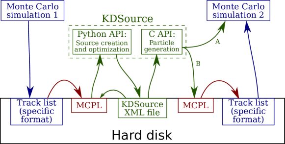
Figure 1: Workflow for the KDSource algorithm. Blue indicates the files and actions related to the Monte Carlo simulation codes, red indicates the MCPL files and related conversions, and green indicates the files and actions related to the KDSource tool.

In the Python API, KDE is implemented using the TreeKDE class of KDEpy library [32]. The main advantage of this library is that it implements adaptive KDE, and that the class TreeKDE includes acceleration via the KDTree structure [33], which reduces the computational cost of evaluating the estimated density and optimizing the KDE source. The proposed tool also uses some utilities from Scikit-Learn [34] (KNN search, K-folding), and CPU parallelization via the joblib library [35].

4 Results

This section is divided into three parts. In the first one, KDSource is tested with a known a priori analytical distribution of correlated variables. To do so, first an analytical multivariate joint distribution is constructed and sampled, after which KDSource is applied to obtain the estimated distribution. Then, both distributions are compared using the Kulback-Leibler divergence. In the subsequent parts, examples of application to the analysis of simulations of real cases are presented. The second part, shows an application of KDSource in a Monte Carlo neutron transport problem to reproduce the spectrum obtained at the LINAC neutron source at CAB (Bariloche, Argentina). In this part, KDSource is used to estimate the joint distribution of the phase-space vector at a certain distance from the source, and then it is sampled to continue the simulation at a further distance. Here it is clear how KDSource is an advantageous tool to accelerate calculations at a great distance between the neutron source and the detector, with accurate results. Finally, in part three, KDSource is used to enhance the convergence of the dose rate map in a neutron tomography facility in the RA-6 research reactor at CAB.

4.1 Verification

In order to evaluate the performance of KDSource, a benchmark test was performed. For this purpose, we generated a multivariate analytical distribution representing a neutron source, with which the variables were sampled, and the KDE method was applied to generate an estimated PDF. The calculation details of this process are described in a Google Colab notebook in the GitHub repository [17].

We chose a 2D-flat source, whose variables (see section 3) are the lethargy $u$, the positions $x,y$, and the direction vector $(d_{x},d_{y},d_{z})=(\sin\theta\cos\varphi,\sin\theta\sin\varphi,\cos\theta)$. The distribution function was constructed so that there were correlated variables, in order to evaluate the ability of the tool to correctly describe it.

The joint distribution function was defined as

$$f(u,x,y,\mu,\varphi)=\left[f_{u,1}(u)f_{x,1}(x)+f_{u,2}(u)f_{x,2}(x)\right]f_{y}(y)f_{\mu}(\mu)f_{\varphi}(\varphi),$$ (6)

where $\mu=\cos\theta$, $f_{u_{1}}$, $f_{u_{2}}$, $f_{x_{1}}$, $f_{x_{2}}$, and $f_{y}$ are normal distributions, $f_{\mu}$ is linear, and $f_{\varphi}$ a constant distribution, as defined below

$$f_{u,i}(u)=\frac{1}{\sqrt{2\pi}\sigma_{\rm u}}\exp{\left[-\frac{(u-\mu_{u,i})^{2}}{2\sigma_{\rm u}^{2}}\right]}$$ (7)

$$f_{x,i}(x)=\frac{1}{\sqrt{2\pi}\sigma_{\rm x}}\exp{\left[-\frac{(x-\mu_{x,i})^{2}}{2\sigma_{\rm x}^{2}}\right]}$$ (8)

$$f_{y}(y)=\frac{1}{\sqrt{2\pi}\sigma_{\rm y}}\exp{\left[-\frac{y^{2}}{2\sigma_{\rm y}^{2}}\right]}$$ (9)

$$f_{\mu}(\mu)=2\mu$$ (10)

$$f_{\varphi}(\varphi)=\frac{1}{2\pi},$$ (11)

where $u$, $x$ and $y$ $\in[-\infty,\infty]$, $\mu>0$ and $\phi\in[0,2\pi]$. The parameters employed in the Gaussian functions are summarized in Table 1.

Parameter	$f_{u,1}$	$f_{u,2}$	$f_{x,1}$	$f_{x,2}$	$f_{y}$
$\mu$	5	9	10	-10	0
$\sigma$	1	1	10	10	10

Table 1: Parameters employed for the definition of the Gaussian functions in Eq.(6).

From the definition of the distribution function, we observe that the lethargy variable $u$ is correlated with the position variable $x$ (the distribution presents two non-aligned Gaussian peaks in the $u-x$ plane). The remaining variables are independent.

A random particle list with the distribution given by Eq. (6) was generated using the numpy library within the Python environment. From this list, the KDE method was applied using KDSource with an optimized bandwidth through the kNN and MLCV methods described in Sect. 3.2. The process was repeated varying the number of particles in the list $N$. In Fig. 2 the MLCV figure of merit (Eq. 4) is shown as a function of the scaling factor of the $h$ vector obtained by kNN, for $N=10^{6}$ training particles, where a clear maximum that defines the optimal bandwidth can be observed. Analytical and estimated distributions were compared using the Kulback-Leibler divergence ($D_{KL}$, see section 2) for different number of sampled particles, and the results are shown in Fig. 3. It can be seen that the $D_{KL}$ is a decreasing function of $N$, meaning that the larger the sample set, the closer is the estimated density to the true PDF. Nevertheless, the information gain decreases with $N$. In fact, the $D_{KL}$ decrease from $10^{5}$ to $10^{6}$ particles is around the 27% of the decrease from $10^{4}$ to $10^{5}$, and the 1% of the same amount from $10^{2}$ to $10^{3}$.

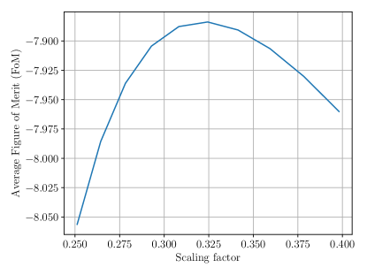
Figure 2: Average Figure of merit of the Maximum Likelihood Cross Validation method, as a function of the scaling factor of the seed bandwidth. The selected normalized bandwidth is the one with the highest average FoM value.

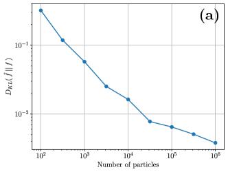
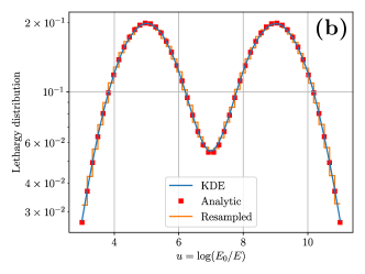
Figure 3: (a) Comparison between analytical and estimated energy spectra. Kulback-Leibler divergence between the analytical and estimated lethargy distribution, as a function of the number of training particles. (b) Comparison between analytical lethargy distribution, estimated distribution (with $N=10^{6}$) and histogram of the resampled particles.

Fig. 3 shows a comparison between the analytical lethargy distribution (red squares), the KDSource estimated distribution with $N=10^{6}$ (blue connected lines), and the histogram obtained by sampling $10^{6}$ new particles from the estimated distribution (orange steps). This figure manifests that the distribution of the sampled points follows accurately the original analytical distribution in the entire energy range. Moreover, we checked the adequate modeling of the distribution correlation between energy and $x$ by plotting the energy spectrum for different ranges of $x$ to see its variation. In Fig. 4 the estimated and analytical distributions are compared for $x<0$ and $x>0$, showing good agreement.

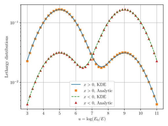
Figure 4: Comparison of the estimated and analytic energy distributions for $x<0$ (red triangles) and $x>0$ (orange squares).

The results presented in this section show that the KDSource tool successfully estimates an analytical correlated joint distribution of the source’s phase space vector, and that it allows to generate new samples from it maintaining the correlations between variables. In the following section, KDSource will be used to produce particles in a Monte Carlo simulation.

4.2 Validation

Next, we will show the use of KDSource in computational simulations applied to neutron spectra measurement experiments made in a pulsed neutron source based on a linear electron accelerator (LINAC). The experiments, described in detail in Ref. [36], correspond to those carried out at the LINAC facility of the Bariloche Atomic Center (CAB) during the 1970s. They consist in the measurement of neutron spectra of pure water at $23\text{\,}\mathrm{\SIUnitSymbolCelsius}$ ($296.15\text{\,}\mathrm{K}$). A simplified sketch of the geometry with its dimensions can be observed in Fig. 5. Fast neutrons are generated by a photonuclear reaction from the bremsstrahlung radiation of the electrons, which, accelerated by the LINAC to an energy of 25 MeV, are stopped by a Fansteel target. The neutrons thus produced are moderated in a $25\text{\,}\mathrm{m}\mathrm{m}$ side H₂O cubic tank, with a re-entrant hole facing a 17 m long flight tube, at the end of which the neutrons are detected.

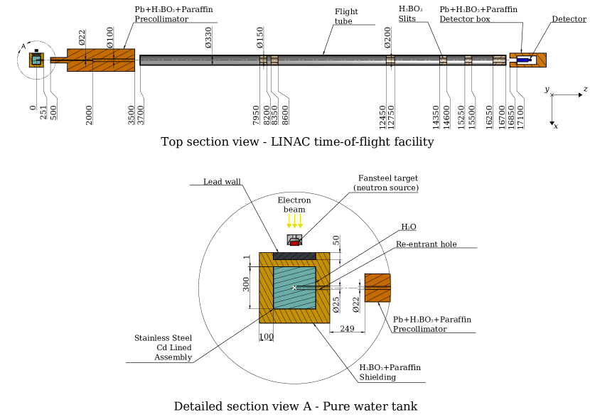
Figure 5: Experimental scheme for the measurement of neutron spectra in pure H₂O. In the upper part a general sketch of the experimental facility is observed. Electrons from the LINAC (not shown in the figure) hit a Fansteel target where fast neutrons are generated. On the left is the moderator consisting of a water cubic container shielded with paraffin and boric acid. The neutrons are extracted through a re-entrant hole facing the flight tube and are detected at a distance of 17 m. On the right the detector placed into a shielding made of lead, boric acid and paraffin is shown. The lower graph shows a detail of the moderator system. The white cross in the lower graph indicates the common coordinate origin for the OpenMC and McStas simulations. All the dimensions shown in the graph are in mm.

The H₂O cubic tank and its shieldings were modeled with the OpenMC Monte Carlo code [29] using the ENDF/B-VII.0 nuclear data library [37], and the flight tube and its slits were modeled with the McStas Monte Carlo code. The calculations were performed starting from a neutron source, modeled as a $3\text{\,}\mathrm{cm}$ radius monodirectional flat disk with a Watt energy distribution

$$S(E)\>dE=c\,e^{-E/a}\sinh\sqrt{b\,E}\>dE,$$ (12)

where $E$ is given in MeV, $a=$$0.38\text{\,}\mathrm{MeV}$, $b=$$7\text{\,}\mathrm{M}\mathrm{eV}^{-1}$, and $c$ is a source particle normalization constant set as $1\text{\,}\mathrm{n}\mathrm{/}\mathrm{s}$. All the particles that cross the surface determined by the start of the re-entrant hole in the OpenMC simulation were saved into an HDF5 file named surface source file (SSF), and only the ones that were directed to the flight tube were filtered and saved into the MCPL format. The coordinate origin common to the OpenMC and McStas simulations, placed at the extreme of the re-entrant hole (center of the surface source), is indicated with a white cross in the lower graph of Fig. 5. The $z$-axis is parallel to the direction of the flight path.

In the experiments, the measured spectra were detected at $17\text{\,}\mathrm{m}$ from the source. This poses a problem for a conventional Monte Carlo simulation since very few of the emitted particles will reach a detector at such a great distance. A conventional OpenMC simulation shows that out of $1\times 10^{10}$ source particles, about $7\times 10^{6}$ cross the reference surface with direction to the flight tube and, only $83$ reach the detector. To overcome this problem and increase the statistics at the detector, KDSource was used to estimate the SSF distribution generated by OpenMC.

Two sources with different lethargy importance factors $\alpha_{u}$ (see Section 3.1) were estimated, resampled, and saved into MCPL format to evaluate their impact in the energy distribution at the end of the flight tube. For the first source (case 1) $\alpha_{u}$ was set to 1 (default value in KDSource) and for the second one (case 2), $\alpha_{u}=10$.

The number of resampled particles was the same as in the original OpenMC SSF, and the resampled particle weights were normalized to preserve the OpenMC integral partial current which is defined as

$$J_{\hat{\mathbf{n}}}^{+}=\dfrac{S_{0}}{N_{\text{sim}}}\sum_{i=1}^{N_{\text{surf}}}w_{i},$$ (13)

where $S_{0}$ is the simulation source factor, $N_{\text{sim}}$ is the total number of source simulated particles, $N_{\text{surf}}$ is the total number of particles that cross out the reference surface with normal direction $\hat{\mathbf{n}}$, and $w_{i}$ are the particle statistical weights. Also, following the notation used in [38], the outgoing normal angular current $j_{\hat{\mathbf{n}}}^{+}(\mathbf{r},E,\hat{\mathbf{\Omega}})$ can be rewritten as

$$j_{\hat{\mathbf{n}}}^{+}(\textbf{r},E,\hat{\mathbf{\Omega}})=J_{\hat{\mathbf{n}}}^{+}\>f(\textbf{r},E,\hat{\mathbf{\Omega}}),$$ (14)

where $f(\textbf{r},E,\hat{\mathbf{\Omega}})$ is a joint PDF obtained as a multivariable histogram weighted with the particle weights.

The lethargy distributions $J_{\hat{\mathbf{z}}}^{+}f(u)$ at the origin of the flight path ($z=$0\text{\,}\mathrm{m}$$) for both cases are shown in Fig. 6, and the values of the integral partial current as a function of the flight length $z$ are shown in Fig. 6. Both figures also show the relative difference between the resampled sources and the OpenMC SSF. Also, a summary with the integral values for different energy and angular ranges is reported in Table 2. The large relative differences shown for the first case can be attributed to the high value of the second derivative in those lethargy regions, as discussed in [11, 39]. The importance factor used for the lethargy variable in the second case reduces the broadening of the lethargy distribution, showing a good agreement with the original SSF. This can also be observed from the integral values shown in Table 2, since the relative difference is larger in the first case than in the second one for all the chosen ranges.

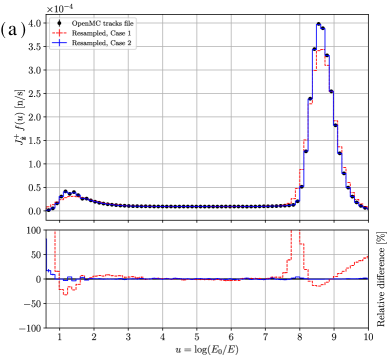
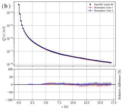
Figure 6: Comparison between the partial current distributions and integral values obtained from the OpenMC SSF and the resampled ones with KDSource code for different lethargy scaling factors ($\alpha_{u}=1.0$ for case 1, and $\alpha_{u}=10.0$ for case 2). (a) Lethargy distribution at the origin of the flight path ($z=0$ m). (b) Integral partial current as a function of the flight length. The lower frames show the relative differences between cases 1 and 2.

Integration range		OpenMC track file	Resampled
			Case 1 ($\alpha_{u}=1.0$)		Case 2 ($\alpha_{u}=10.0$)
$\Delta E$ [eV]	$\Delta\mu$	$J^{+}_{\hat{\mathbf{z}}}$ [n/s]	$J^{+}_{\hat{\mathbf{z}}}$ [n/s]	Difference [%]	$J^{+}_{\hat{\mathbf{z}}}$ [n/s]	Difference [%]
Total	Total	$4.226(2)\times 10^{-4}$
[1$\times 10^{-5}$, 0.3]	Total	$3.281(1)\times 10^{-4}$	$3.265(1)\times 10^{-4}$	$-0.47(6)$	$3.280(1)\times 10^{-4}$	$-0.01(6)$
	[0.0, 0.5]	$8.316(7)\times 10^{-5}$	$8.268(7)\times 10^{-5}$	$-0.6(1)$	$8.369(7)\times 10^{-5}$	$0.6(1)$
	[0.5, 1.0]	$2.449(1)\times 10^{-4}$	$2.439(1)\times 10^{-4}$	$-0.43(7)$	$2.445(1)\times 10^{-4}$	$-0.23(7)$
[0.3, 2$\times 10^{7}$]	Total	$9.45(1)\times 10^{-5}$	$9.60(1)\times 10^{-5}$	$1.6(1)$	$9.46(1)\times 10^{-5}$	$0.0(1)$
	[0.0, 0.5]	$3.134(6)\times 10^{-5}$	$3.213(4)\times 10^{-5}$	$2.5(2)$	$3.198(4)\times 10^{-5}$	$2.0(2)$
	[0.5, 1.0]	$6.319(8)\times 10^{-5}$	$6.389(6)\times 10^{-5}$	$1.1(2)$	$6.258(6)\times 10^{-5}$	$-1.0(2)$

Table 2: Comparison between integral $J^{+}_{\hat{\mathbf{z}}}$ values obtained from the OpenMC SSF and the resampled ones with KDSource code for different ranges of energy ($\Delta E$) and polar angle direction ($\Delta\mu$), indicated in the first two columns (“Total” indicating intergation over the whole variable range). The first value for $J_{\hat{\mathbf{z}}}^{+}$ corresponds to the integral partial current, i.e. integrated over all the phase space variables domain, and it is equal for both cases due to the normalization chosen.

Fig. 7 shows the comparison between the original distributions of the SSF variables and those obtained from the resampling of the estimated distribution (case 2). Also, for each variable the relative difference between the resampled histogram and the OpenMC particle lists histogram is shown. To verify the correlation between the variables, different domains of interest were used for each distribution. The subscript $\Delta(...)$ of the PDF function in ordinates indicates that a partial integration has been performed in the variables in parentheses. As this figure shows, the largest differences between original SSF and resampled distributions are generally less than 20%. In particular, the relative difference increases when the distributions tends to zero at the domain borders, attributable this also to a high second derivative and to the lower statistics in those regions of the phase space. This figure also shows that the correlations for the lethargy, position, direction are respected.

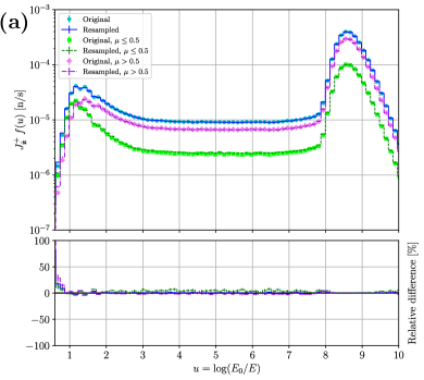
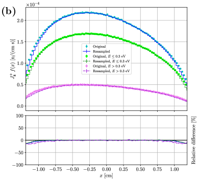
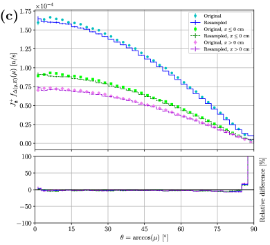
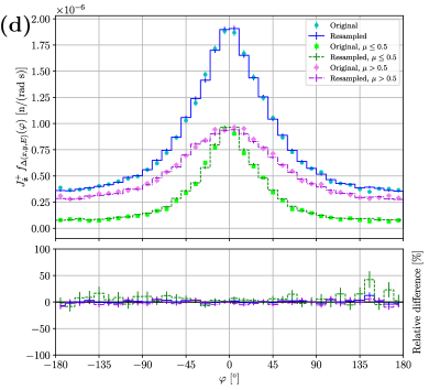
Figure 7: Partial current distributions of the neutrons emitted by the source obtained from the OpenMC SSF and the resampled ones with KDSource code. In all the lower frames relative differences are shown for comparison. (a) Lethargy distribution, where $x$ and $y\in(-\infty,\infty)$ and $\varphi\in[0,2\pi$]. (b) Position distribution, where $y\in(-\infty,\infty)$, $\mu\in[0,1]$ and $\varphi\in[0,2\pi]$. (c) Polar angle direction distribution, where $y\in[-0.25,0.25]$ cm, $E\in[0,0.3]$ eV and $\varphi\in[0,2\pi]$. (d) Azimuthal angle direction distribution, where $x$ and $y\in[-0.25,0.25]$ cm and $E\in[0.3,\infty)$ eV.

Finally, in Fig. 8, the experimental spectra [40] is compared with the ones obtained with McStas using the original SSF and the resampled one with KDSource (case 2). The number of particles sampled with the distribution estimated by KDSource was 1000 times larger than that of the original OpenMC SSF. The agreement between the experimental and the sampled spectra is remarkable, which is evidenced by the fact that the relative bin-to-bin difference values are always below 20%, as shown in the lower frame. Figure 8 also shows that in a common Monte Carlo simulation, there are energies that are never recorded due to the finite number of particles, a situation that is overcome with the use of KDSource.

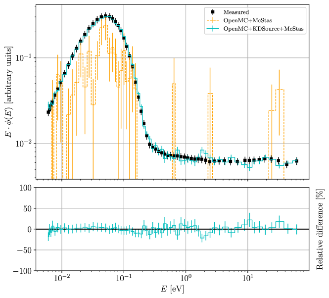
Figure 8: Comparison between the experimental spectrum (black squares) and those calculated by a standard OpenMC simulation (orange bars with errors) and by combining OpenMC, McStas and KDSource. Relative differences between experimental measurements and KDSource results are shown for comparison in the lower frame.

4.3 Application

As an application case of the method presented here, we show its use in transport calculations using the OpenMC code, employed in the design of an instrument using a neutron beam of an experimental reactor. The case studied is the neutrography facility of the RA-6 reactor of the Bariloche Atomic Center (Argentina). The goal is to map the neutron flux inside the instrument housing to perform the dosimetry evaluation. A first simulation using OpenMC starting from the reactor core reveals the difficulty in obtaining an adequate dose rate statistic (see Fig. 9). To improve the calculations, KDSource was used to evaluate the source defined at surface S1 of the reactor neutron beam port entrance. For this, the simulation was employed to generate a track list of $N=5\times 10^{4}$ neutrons at surface S1.

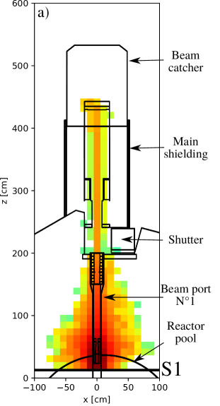
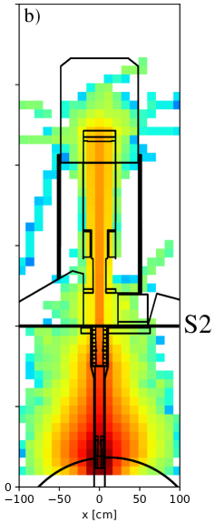
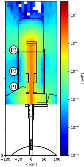
Figure 9: Neutron dose rate map of RA6 reactor’s conduit that leads to the neutrography facility. Samples from Kernel density estimations of the dose rate map at different distances (S1 and S2) from the source are depicted. (a) Core simulation. source. (b) First KDE source. (c) Second KDE source.

The application of KDSource served to estimate the joint PDF of the neutron phase vector components. This allowed to perform a second simulation with $N=5\times 10^{6}$ neutrons generated from the estimated distribution at S1. The dose rate map thus obtained can be seen in Fig. 9. Although the map has improved in the vicinity of the beam port with respect to that of Fig. 9, it has not yet converged in the region downstream the tube exit (referred as surface S2 in fig. 9). Since our goal is to determine a dose rate map in the surroundings of the instrument, reliable enough to be compared with measured dose rates, we generated a new particle list at surface S2 consisting in $N=1\times 10^{4}$ neutrons registered from the previous simulation of the KDE source at S1, and performed a third simulation. The new source distribution at surface S2 thus generated keeps the correlations between variables of the phase space vector. The dose rate map was obtained by resampling $1\times 10^{7}$ neutrons from S2. The result is shown in fig. 9. Thus, an efficient propagation of the source distribution (with the corresponding correlations between variables) at a greater distance along the beamline can be achieved, allowing a better estimation of the dose rate map far away of the reactor core.

Finally, the simulation’s results of the dose rate map shown in fig. 9 were contrasted with experimental measurements taken at the points P1, P2, and P3 near the main shielding structure (see fig. 9). The measurements were carried out for a radiological survey of the facility, in order to detect surrounding locations that require protected actions such as improved shieldings, barrier placement and standards of use. Measured values of the neutron dose rate and values obtained by simulation are shown in table 3 for three points.

Point	Neutron dose rate $[\mu Sv/h]$		Relative Error [%]
	Experimental	Calculation
P1	30	46	53
P2	25	29	16
P3	120	125	4

Table 3: Neutron dose rate comparison of RA6 reactor’s beamport.

As can be seen, the values obtained from the simulation are consistent with the experimental values, and the consistency increases with the distance to the surface S2. It is also interesting to note that the dose rate at point P3, which is the farthest from the source is higher than at points P1 and P2 due to the backscattering in the beam catcher. This feature is being correctly represented in the simulation because KDE is allowing to sample a large amount of neutrons from the surface S2, allowing the map to converge adequately.

5 Discussion and conclusions

In this work we presented KDSource, a new tool for generating source distributions based on the kernel density estimation (KDE) method. The implemented algorithm automatically optimizes a KDE model based on a list of particles recorded at an intermediate position of a Monte Carlo simulation, normally the input of a radiation beam, thus estimating the current density distribution there. As already shown in previous similar implementations [8, 9, 10], this technique clearly benefits the tally computation in beam simulations compared to direct use of the particle list. The tool aims to simplify the application of the KDE method with respect to the mentioned implementations, reducing the required user expertise and the engineering hours, by providing an abstract user interface.

The properties and usefulness of the KDSource tool were studied in three different problems. The first one, referred as verification, allowed to check some basic properties of the KDSource algorithm, such as the convergence of the estimated distribution to the real density, and the adequate correlation modeling. This was possible because, in this analytical problem, the real density was known. The second problem provided a demonstration of KDSource’s benefits in a real Monte Carlo simulation, significantly increasing the statistics at the end of a neutron beam. In this case validity of the KDE source was verified by comparing it with the track source at the points where both had sufficient statistics, and with the experimental results. Finally, in the application problem the KDSource algorithm was used to solve an actual problem of interest in a research reactor neutron beam, allowing shielding calculations far away from the core, with reasonable agreement with experimental results.

From a more theoretical point of view, the advantages of the KDSource algorithm, observed in the last two problems, can be understood as follows. In a Monte Carlo simulation, uncertainties in the sources distribution result in systematic errors in the computed tallies. Sensitivity is maximal in vacuum propagation problems, where flux maps depend strongly on the source, and not in the properties of the medium (as in moderation problems). In such cases, KDSource improves the simulation by reducing the variances of the tallies caused by the statistical fluctuations of the particle list, which could be noticeable with a tracks source. Therefore, the KDSource tool is expected to be useful on applications with strong vacuum propagation, specially beam simulations and associated shielding calculations. Furthermore, if the tracks list on which the KDE model is fitted is independent of the downstream problem, which is common in beams, the KDE source can be reused with different downstream configurations, increasing the benefits of the methodology.

In future works the capabilities of KDSource are expected to be extended in several ways. This includes the possibility of choosing between different kernel functions (Epanechnikov, Gaussian, triangular, Tophat, Exponential, etc.), the inclusion of other possible bandwidth optimization methods, such as Least-Squares Cross-Validation, and further source optimization techniques like source-biasing. It is also important to complete the documentation of all the functionalities of KDSource, following the usual software standards. In addition, there are other application problems that can be explored, such as the calculation of coupled optics shielding around neutron guides, and the modeling of neutron activation sources. Finally, regarding the statistical properties of the implemented algorithm, a practical procedure to determine the minimum number of training particles required to properly fit a KDE model is left as a possibility for future improvements.

6 Acknowledgements

Funding from Universidad Nacional de Cuyo (Project 06-C563), ANPCYT (Agencia Nacional de Promoción Científica y Tecnológica - Argentina) (PICT 2019 - 02665) and CNEA (Argentine National Commission of Atomic Energy) are gratefully acknowledged.

References

- Jazbec et al. [2021] A. Jazbec, B. Kos, K. Ambrožič, L. Snoj, Dose rate calculations at beam tube no. 5 of the JSI TRIGA mark II research reactor using Monte Carlo method, Applied Radiation and Isotopes 168 (2021) 109510.
- Mosher et al. [2013] S. W. Mosher, S. R. Johnson, A. M. Bevill, A. M. Ibrahim, C. R. Daily, T. M. Evans, J. C. Wagner, J. O. Johnson, R. E. Grove, ADVANTG—an automated variance reduction parameter generator, ORNL/TM-2013/416 Rev 1 (2013).
- Kittelmann et al. [2017] T. Kittelmann, E. Klinkby, E. B. Knudsen, P. Willendrup, X.-X. Cai, K. Kanaki, Monte carlo particle lists: MCPL, Computer Physics Communications 218 (2017) 17–42.
- Willendrup and Lefmann [2020] P. K. Willendrup, K. Lefmann, McStas (ii): An overview of components, their use, and advice for user contributions, Journal of Neutron Research (2020) 1–21.
- Ersez et al. [2018] T. Ersez, F. Esposto, H. Lake, N. R. de Souza, Validation of the Radiological Shielding for the EMU Neutron Spectrometer at the OPAL Reactor, in: Proceedings of the International Conference on Neutron Optics (NOP2017), 2018, p. 011006.
- Fairhurst Agosta [2017] R. E. Fairhurst Agosta, Detailed neutronic calculus of the beams and neutrons guides of the RA-10, Master’s thesis, Universidad Nacional de Cuyo, 2017.
- Ayala [2019] J. E. Ayala, Implementation of a shielding radiation calculation line for RA-10 reactor, Master’s thesis, Universidad Nacional de Cuyo, 2019.
- Tyagi et al. [2006] N. Tyagi, W. R. Martin, J. Du, A. Bielajew, I. J. Chetty, A proposed alternative to phase-space recycling using the adaptive kernel density estimator method, Medical physics 33 (2006) 553–560.
- Banerjee [2010] K. Banerjee, Kernel Density Estimator Methods for Monte Carlo Radiation Transport., Ph.D. thesis, University of Michigan, 2010.
- Burke [2016] T. Burke, Kernel Density Estimation Techniques for Monte Carlo Reactor Analysis., Ph.D. thesis, University of Michigan, 2016.
- Scott [2015] D. W. Scott, Multivariate density estimation: theory, practice, and visualization, John Wiley & Sons, 2015.
- Silverman [1986] B. W. Silverman, Density Estimation for Statistics and Data Analysis, Chapman & Hall, London, 1986.
- Bartlett [1963] M. S. Bartlett, Statistical estimation of density functions, Sankhyā: The Indian Journal of Statistics, Series A (1961-2002) 25 (1963) 245–254.
- Silverman [1998] B. Silverman, Density Estimation for Statistics and Data Analysis, 1 ed., Routledge, Boca Raton, 1998. doi:https://doi.org/10.1201/9781315140919.
- Terrell and Scott [1992] G. R. Terrell, D. W. Scott, Variable Kernel Density Estimation, The Annals of Statistics 20 (1992) 1236 – 1265. doi:10.1214/aos/1176348768.
- Kullback and Leibler [1951] S. Kullback, R. A. Leibler, On Information and Sufficiency, The Annals of Mathematical Statistics 22 (1951) 79 – 86. doi:10.1214/aoms/1177729694.
- Abatte et al. [2021] I. O. Abatte, N. Schmidt, Z. Prieto, J. I. Robledo, J. Dawidowski, A. Márquez, J. I. Márquez, KDSource, a tool for the generation of Monte Carlo particle sources using kernel density estimation, 2021. URL: https://github.com/KDSource/KDSource.
- Kittelmann and et. al. [2017] T. Kittelmann, et. al., Monte Carlo Particle Lists: MCPL, Computer Physics Communications 218 (2017) 17–42.
- X-5 Monte Carlo Team [2003] X-5 Monte Carlo Team, MCNP - Version 5, Vol. I: Overview and Theory, 2003. Report LA-UR-03-1987.
- Pelowitz [2011] D. Pelowitz, MCNPX Users Manual Version 2.7.0, 2011. Report LA-CP-11-00438.
- Werner [2017] C. Werner, MCNP Users Manual - Code Version 6.2, 2017. Report LA-UR-17-29981.
- Sato et al. [2018] T. Sato, Y. Iwamoto, S. Hashimoto, T. Ogawa, T. Furuta, S. ichiro Abe, T. Kai, P.-E. Tsai, N. Matsuda, H. Iwase, N. Shigyo, L. Sihver, K. Niita, Features of Particle and Heavy Ion Transport code System (PHITS) version 3.02, Journal of Nuclear Science and Technology 55 (2018) 684–690. doi:10.1080/00223131.2017.1419890.
- Agostinelli and et. al. [2003] S. Agostinelli, et. al., Geant4—a simulation toolkit, Nuclear Instruments and Methods in Physics Research Section A: Accelerators, Spectrometers, Detectors and Associated Equipment 506 (2003) 250–303. doi:https://doi.org/10.1016/S0168-9002(03)01368-8.
- Lefmann and Nielsen [1999] K. Lefmann, K. Nielsen, McStas, a general software package for neutronray-tracing simulations, Neutron News 10 (1999) 20–23. doi:10.1080/10448639908233684.
- Willendrup et al. [2004] P. Willendrup, E. Farhi, K. Lefmann, McStas 1.7 - a new version of the flexible Monte Carlo neutron scattering package, Physica B: Condensed Matter 350 (2004) E735–E737. doi:https://doi.org/10.1016/j.physb.2004.03.193, proceedings of the Third European Conference on Neutron Scattering.
- Willendrup et al. [2014] P. Willendrup, E. Farhi, E. Knudsen, U. Filges, K. Lefmann, McStas: Past, Present and Future, Journal of Neutron Research 17 (2014) 35 – 43. doi:10.3233/JNR-130004.
- Bergbäck Knudsen et al. [2013] E. Bergbäck Knudsen, A. Prodi, J. Baltser, M. Thomsen, P. Willendrup, M. Sanchez Del Rio, C. Ferrero, E. Farhi, M. Haldrup, A. Vickery, R. Feidenhans’l, K. Mortensen, M. Nielsen, H. Poulsen, S. Schmidt, K. Lefmann, McXtrace: A Monte Carlo software package for simulating X-ray optics, beamlines and experiments, Journal of Applied Crystallography 46 (2013) 679–696. doi:10.1107/S0021889813007991.
- Brun et al. [2015] E. Brun, F. Damian, C. Diop, E. Dumonteil, F. Hugot, C. Jouanne, Y. Lee, F. Malvagi, A. Mazzolo, O. Petit, J. Trama, T. Visonneau, A. Zoia, TRIPOLI-4®, CEA, EDF and AREVA reference Monte Carlo code, Annals of Nuclear Energy 82 (2015) 151–160. doi:https://doi.org/10.1016/j.anucene.2014.07.053.
- Romano and Forget [2013] P. K. Romano, B. Forget, The OpenMC monte carlo particle transport code, Annals of Nuclear Energy 51 (2013) 274–281.
- Duin [1976] R. Duin, On the Choice of Smoothing Parameters for Parzen Estimators of Probability Density Functions, IEEE Transactions on Computers C-25 (1976) 1175–1179. doi:10.1109/TC.1976.1674577.
- Refaeilzadeh et al. [2016] P. Refaeilzadeh, L. Tang, H. Liu, Cross-Validation, Springer New York, New York, NY, 2016, pp. 1–7. doi:10.1007/978-1-4899-7993-3_565-2.
- Odland [2018] T. Odland, KDEpy, 2018. URL: https://kdepy.readthedocs.io/en/latest/.
- Weinberger [2018] K. Weinberger, Machine Learning for Intelligent Systems, cap. 16: KD Trees, 2018. Accesed: 4-sep-2021.
- Pedregosa et al. [2011] F. Pedregosa, G. Varoquaux, A. Gramfort, V. Michel, B. Thirion, O. Grisel, M. Blondel, P. Prettenhofer, R. Weiss, V. Dubourg, J. Vanderplas, A. Passos, D. Cournapeau, M. Brucher, M. Perrot, E. Duchesnay, Scikit-learn: Machine learning in Python, Journal of Machine Learning Research 12 (2011) 2825–2830.
- Joblib Development Team [2020] Joblib Development Team, Joblib: running python functions as pipeline jobs, 2020. URL: https://joblib.readthedocs.io/.
- Abbate et al. [1974] M. Abbate, L. Remez, J. Lolich, J. Volkis, Facility for the measurement of neutron spectra by the time-of-flight method, Technical Report, Comisión Nacional de Energía Atómica, 1974.
- Chadwick et al. [2006] M. Chadwick, P. Obložinskỳ, M. Herman, N. Greene, R. McKnight, D. Smith, P. Young, R. MacFarlane, G. Hale, S. Frankle, et al., ENDF/B-VII. 0: next generation evaluated nuclear data library for nuclear science and technology, Nuclear data sheets 107 (2006) 2931–3060.
- Duderstadt and Martin [1979] J. J. Duderstadt, W. R. Martin, Transport theory., Transport theory (1979).
- Stoker [1993] T. M. Stoker, Smoothing bias in density derivative estimation, Journal of the American Statistical Association 88 (1993) 855–863.
- Abbate et al. [1976] M. Abbate, J. Lolich, T. Parkinson, Neutron Thermalization in Light Water—Measurement and Calculation of Spectra, Nuclear Science and Engineering 60 (1976) 471–477.