Correlating exciton coherence length, localization, and its optical lineshape. I. a finite temperature solution of the Davydov soliton model

Abstract

The lineshape of spectroscopic transitions offer windows into the local environment of a system. Here, we present a novel approach for connecting the lineshape of a molecular exciton to finite-temperature lattice vibrations within the context of the Davydov soliton model (A. S. Davydov and N. I. Kislukha, Phys. Stat. Sol. 59,465(1973)). Our results are based upon a numerically exact, self-consistent treatment of the model in which thermal effects are introduced as fluctuations about the zero-temperature localized soliton state. We find that both the energy fluctuations and the localization can be described in terms of a parameter-free, reduced description by introducing a critical temperature below which exciton self-trapping is expected to be stable. Above this temperature, the self-consistent ansatz relating the lattice distortion to the exciton wavefunction breaks down. Our theoretical model coorelates well with both experimental observations on molecular J-aggregate and resolves one of the critical issues concerning the finite temperature stability of soliton states in alpha-helices and protein peptide chains.

I Introduction

One of the the fundamental issues in the materials science of disordered semiconductors is in the unravelling optical and electronic properties from disordered energy landscapes and correlating these to complex solid-state microstructures. In polymeric semiconductors in particular, the structure-property interdependence is such that the excitation spectral line shapes are governed by the interplay between inter- and intra-chain electronic interactions both of which are highly sensitive to the local microstructures of the system. Within the Kubo-Anderson model, the homogeneous lifetime is related to the variance or fluctuations in the spectroscopic energy level and the correlation time of the fluctuations via. $T_{2}=(\Delta^{2}\tau_{c})^{-1}$. [1, 2, 3] It is desirable to relate both $\Delta^{2}$ and $\tau_{c}$ to properties of the material substrate.

It was suggested in Ref.4 following arguments in Ref. 5 that the lineshape in polycrystaline polymeric semiconductors could be interpreted in the context of a weakly coupled aggregate model simple two-dimensional free-exciton model of an aggregate composed of polymer chains of with a persistence length $\ell_{x}$ that are assembled to form a lamellar stack of persistence length $\ell_{y}$. Excitonic coupling effects, both along and between chains can be described by an intrachain (parallel) hopping integral $J_{\parallel}$, and an interchain (perpendicular) hopping integral $J_{\perp}$. Using a two-dimensional free exciton model we showed the ratio of the homogeneous linewidths of the isolated (single chain) to the aggregate is related to delocalization along each direction.

$$r=\frac{\gamma_{iso}}{\gamma_{agg}}=\frac{J_{\parallel}}{J_{\perp}}\left(\frac{\ell_{\perp}}{\ell_{\parallel}}\right)^{2}$$ (1)

Consequently, by taking the ratio of the homogeneous line-widths for the isolated vs. aggregate system, one obtains a succinct measure of the localization of the exciton. However, the model is based upon a simple free-exciton model, essentially a particle-in-a-box, where one expands the approximately parabolic energy bands about the super-radiant transition giving $\gamma_{homog}\propto|J|/(\ell)^{2}$. This is expected to be true in the high-temperature limit where the exciton momentum is no longer a good quantum number and localization is due to dynamical disorder. At low temperature, however, the lineshape reflects the static localization due to the static disorder. This trend is observed in studies of cyanine dye J-aggregate films (Ref. 5) in which it is reported that the dynamical scattering limit persists even down to 9K with no transition to the static disorder limit.

In this paper, we revisit this model with the goal of correlating the exciton lineshape with its localization length taking into account static and dynamic disorder at finite temperature. For this, we present exciton models in which energy fluctuations are introduced in terms of local site energy fluctuations and include the effect of self-trapping whereby the initial exciton localization is due to coupling to the lattice phonons. We then introduce finite-temperature fluctuations around the $T=0K$ STE and consider how the STE picture is modified at finite temperature. Our results are based upon a numerically exact, self-consistent treatment of the Davydov soliton model[6] in thermal effects are introduced as fluctuations about the zero-temperature soliton state. We find that both the energy fluctuations and the exciton localization can be described in terms of a parameter-free, reduced description by introducing a critical temperature below which exciton self-trapping is expected to be stable. Above this temperature, the self-consistent ansatz relating the lattice distortion to the exciton wavefunction breaks down.

II Theoretical model

The central issue of this paper concerns the connection between dynamic disorder and the homogeneous line width of molecular excitons. To set the framework for our discussion, we begin with a basic finite 1D lattice exciton model with weak diagonal disorder,

$$H =\sum_{n=0}^{N-1}(E_{n}+\delta\epsilon_{n}(t))|n\rangle\langle n|$$ (2)

$$+J\sum_{n=0}^{N-1}(|n+1\rangle\langle n|+|n\rangle\langle n+1|,$$ (3)

in which $|n\rangle$ represents a local excitation on site $n$ with energy $E_{n}+\delta\epsilon_{n}(t)$ and $J$ is the hopping integral between nearest neighbors. For J-aggregates, $J<0$ such that the lowest-energy exciton transition corresponds to a super-radiant state. We introduce a time-dependent local energy fluctuation $\delta\epsilon_{n}(t)$ which we shall assume arises from stochastic process describing the local environment. For now, we leave that processes unspecified but assume that $E_{n}=E_{o}$ for a homogeneous lattice and that $J^{2}>>\langle\delta\epsilon^{2}\rangle$. Under this assumption, we can easily diagonalize the static part:

$$E_{k}=E_{o}+2J\cos\left(\frac{\pi k}{N+1}\right)$$ (4)

where $k=1,\cdots N$ is a quantum number and with states

$$|k\rangle=\left(\frac{2}{N+1}\right)^{1/2}\sum_{n=1}^{N}\sin\left(\frac{kn\pi}{N+1}\right)|(n-1)\rangle$$ (5)

In the high-temperature limit, fluctuations produce excitations about the $T=0K$ exciton which we can include by expanding $E_{k}$ about the lowest-energy transition (corresponding to quantum number $k=1$) and introducing fluctuations $k-1\to\delta k(t)$

$$E(t) =\left(E_{o}+2J\cos(\ell^{-1})\right)-\delta k(t)\frac{2J}{\ell}\sin(\ell^{-1})+\cdots$$ (6)

where we write $\ell^{-1}=\pi/(N+1)$ which becomes small as the number of sites $N$ increases. Thus, we can write the exciton energy fluctuations as

$$\delta E(t) \approx\frac{2|J|}{\ell^{2}}\delta k(t).$$ (7)

This model assumes that the exciton is in some thermal population driven by contact with a finite temperature bath. We can use the fluctuation/dissipation theorem,

$$\langle\delta E(t)\delta E(0)\rangle\propto k_{B}T\frac{2|J|}{\ell^{2}}Z(t),$$ (8)

where the memory kernel $Z(t)$ is the Fourier transform of the spectral density associated with the system/bath interaction.[7, 8] Consequently, the homogeneous lineshape is expected to increase with temperature. Both of these trends are apparent in Ref.5 and Ref. 4.

However, the model is highly unsatisfactory since it imposes a localization length, $\ell$, on the exciton and does not account for lattice reorganization effects which would contract the exciton which would suggest that the homogeneous linewidths of the photoemission spectra would be broad compared to the absorption spectra. This prompts us to consider a unified model under which the coupling between the lattice and the exciton is treated under a non-perturbative and self-consistent framework at both $T=0K$ and at finite temperature.

II.1 Self-trapped excitons

We now consider the competition between noise and localization due to the relaxation of the lattice about the excitation. Here, we will remain in the exchange narrowing regime and treat the stochastic contribution as a perturbative correction to the exciton energy. As above, taking the local fluctuations to be site-wise statistically uncorrelated, the exciton energy correlation is simply proportional to the IPR for the state, viz.

$$\langle\delta E(t)\delta E(0)\rangle=\sigma^{2}e^{-t/\tau_{c}}\ell^{-1}$$ (9)

For polymers, we need a non-perturbative approach whereby the lattice relaxation and the exciton are treated on co-equal footings. For this, we append to the lattice model described above a term for the harmonic motion of the lattice sites from their equilibrium positions

$$H_{latt}=\sum_{n}\left(\frac{m}{2}\dot{u}_{n}^{2}(t)+\frac{k}{2}(u_{n}-u_{n+1})^{2}\right)$$ (10)

whereby $m$ is the mass, $u_{n}$ is the site displacement, and $k$ is the spring constant. We consider the lattice/exciton interaction to be specified by

$$H_{int}=\chi\sum_{n}(u_{n+1}-u_{n-1})|n\rangle\langle n|$$ (11)

which accounts for the fact that an excitation on site $|n\rangle$ induces either an attractive $(\chi<0)$ or repulsive $(\chi>0)$ interaction that either compresses or expands the lattice about a local exciton. This is the well-known Davydov model used to describe solitons in protein peptide $\alpha$-helices. [6, 9, 10] For completion, we discuss the derivation and mathematical solutions of the model and point out how the model connects the exciton lineshape.

The exciton/lattice equations of motion can now be obtained by writing the exciton state as

$$\langle n|\phi(t)\rangle=\phi_{n}(t)$$ (12)

and substituting this into the Schrödinger equation,

$$i\hbar\partial_{t}\phi_{n} =(E+H_{latt}+\chi(u_{n+1}-u_{n-1})\phi_{n}$$

$$-J(\phi_{n-1}+\phi_{n+1})$$ (13)

$$m\ddot{u}_{n} =k(u_{n+1}-2u_{n}+u_{n-1})$$

$$+\chi(|\phi_{n+1}|^{2}-|\phi_{n-1}|^{2}).$$ (14)

Accordingly, this can be cast into continuum form,

$$i\hbar\partial_{t}\phi(x) =\left(E_{o}+2\chi\nabla u\right)\phi(x)-J\nabla^{2}\phi(x)$$ (15)

$$\ddot{u}-\frac{k}{m}\nabla^{2}u =2\frac{\chi}{m}\nabla|\phi|^{2},$$ (16)

where the energy $E_{o}$ is given by

$$E_{o}=E-2J+\frac{1}{2}\int_{-\infty}^{\infty}\left(m\ddot{u}^{2}+ku^{\prime\prime}\right)dx.$$ (17)

In the continuum limit, we see that the lattice is described as a wave equation that driven by its coupling to the quantum motion of the exciton. With this in mind, we seek traveling wave solutions of the form $u(x,t)=u(x-vt)$ where $v$ is the phonon group velocity. Substituting this into the wave equation produces

$$\nabla u=-\frac{2\chi}{k(1-s^{2})}|\phi|^{2}$$ (18)

where $s=v/c$ is the speed relative to the speed of sound of the lattice. One can then introduce this last term into the Schrödinger equation:

$$i\hbar\partial_{t}\phi=\left(-J\nabla^{2}-g|\phi|^{2}-E_{o})\right)\phi$$ (19)

with $g=4\chi^{2}/(k(1-s^{2}))$. This is the non-linear Schrödinger equation (NLSE) and for $g>0$, one obtains a “bright” soliton,

$$\phi_{bright}(x)=\sqrt{\frac{1}{2\lambda}}\frac{1}{\cosh(x/\lambda)},$$ (20)

in which the exciton is localized over a finite spatial region with eigenvalue $\mu=g^{2}/16J$ and $\lambda=4J/g$.

As above, we can compute the IPR for the case where $s=0$

$$IPR=\frac{1}{3\lambda}=\frac{g}{12J}=\frac{1}{3J}\frac{\chi^{2}}{k}.$$ (21)

This reveals how exciton delocalization (increasing with $J$) and exciton/phonon coupling, which localizes the state with increasing $\chi$ compete to determine the exciton localization length. We need to bear in mind that this is a $T=0K$ result and we can not make the perturbative separation between the exciton localization length and the local site energy fluctuations as we did above. Finally, the IPR is related to the the lattice reorganization energy (c.f. Ref. 10 Eq. 1.12)

$$E_{B} =\frac{|g|}{24}\int\phi^{4}(x)dx$$

$$=\frac{g^{2}}{18J}.$$ (22)

As a brief aside, our result differs from that of Ref. 10 because of the difference in the form of the exciton/phonon interaction Hamilonian. However, it allows us to directly relate the parameters of our model to observed spectroscopic quantities.

II.2 STE Energy fluctuations at finite temperature

To proceed, we assume that the lattice can be treated within the continuum limit and that the traveling wave condition can still be applied. Also, we make the semiclassical ansatz that exciton wavefunction takes the form

$$\phi(x)=\sqrt{n(x)}e^{-i\mu t}$$

where $n(x)$ is the exciton density and we consider only the self-trapped or bright-soliton case. Any fluctuations in the system must correspond to excitations from the bright soliton state. Assuming the $T=0K$ state to be good reference, we introduce $T\neq 0$ fluctuations by writing

$$\phi(r,t) =\phi_{o}(r,t)+\delta\phi(r,t).$$ (23)

We now write the fluctuations as

$$\delta\phi=e^{-i\mu t}\left(u(r)e^{-i\omega t}-v^{*}(r)e^{+i\omega t}\right),$$ (24)

which we then insert into the NLSE above. Linearizing with respect to the fluctuations, we obtain a set of coupled differential equations which can be cast into the form

$${\bf T}\cdot{\bf y}=\hbar\omega{\bf y}$$ (25)

where $T$ is the anti-Hermitian matrix

$${\bf T}=\left[\begin{array}[]{cc}A&B\\ -B^{*}&-A\end{array}\right]$$ (28)

with

$$A =(-J\partial_{x}^{2}-2gn(x)-\hbar\mu)$$ (29)

$$B =-gn(x)$$ (30)

and

$${\bf y}=\left[\begin{array}[]{c}u(x)\\ v(x)\end{array}\right]$$ (33)

are the two-component eigenfunction solutions. Mathematical properties of the ${\bf T}$ matrix and its eigenspectrum are discussed in the Appendix.

To proceed, we construct numerical solutions of Eq. 25 using the NDEigensystem[] package implemented in Mathematica (v 12).[11] The approach uses finite element discretization over a finite range of $x$, corresponding to $x\in 8[-\lambda,\lambda]$ to insure the stationary state boundary condition $y(x)=0$ as $x\to\pm\infty$ and a fine enough mesh to converge the eigenvalues to a satisfactory tolerance. For parameters, we choose our energy unit to be $J$, which determines the band-width of the free exciton, and consider solutions with increasing values of the coupling constant $g$. The output consists of numerical eigenvalues and two-component eigenvectors.

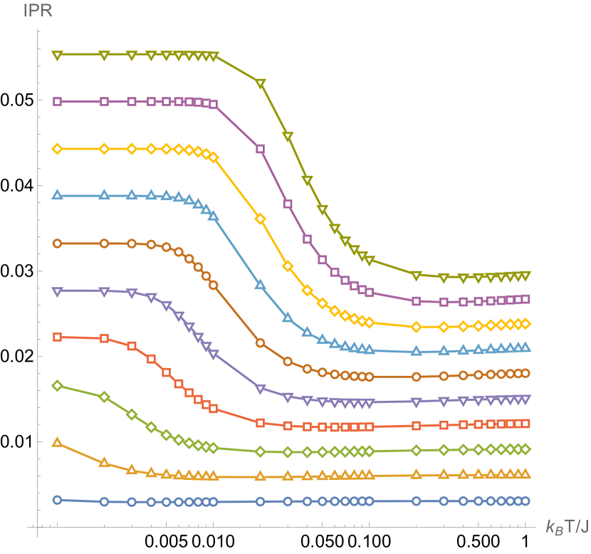
Figure 1: IPR vs. Temperature with increasing values of the coupling parameter $g$. As the temperature increases, the STE undergoes a transition from a localized to delocalized state.

Our model assumes that the fluctuations $\delta\psi$ are from the thermal fluctuations of the lattice itself. With this in mind, we construct the thermal density matrix for the exciton as

$$n_{T}(x)=n_{o}(x)+\frac{1}{Z}\sum_{i}e^{-\hbar\beta\omega_{i}}\delta n_{i}(x)$$ (34)

where the sum is over all positive real eigenvalues of the stability equations from above, $Z$ is the partition function

$$Z=\sum_{i}e^{-\hbar\beta\omega_{i}}$$ (35)

taken by summing over positive real eigenvalues and $\delta n_{i}(x)$ is the (normalized) fluctuation density contribution given by

$$\delta n_{i}(x) ={\bf y}_{i}(x)\cdot\sigma_{3}\cdot{\bf y}_{i}(x)$$ (36)

$$=|u_{i}(x)|^{2}-|v_{i}(x)|^{2}.$$ (37)

Correspondingly, we define the IPR by integrating over the (normalized) total density,

$$IPR=\int n_{T}^{2}(x)dx.$$ (38)

Figure  1 shows the variation of the IPR for the STE as a function of increasing temperature for various choices of $g$ ranging from $g/J=0.1$ to $g/J=1$. For very weak exciton/lattice couplings, the IPR shows little to no variation with temperature and as the coupling increases there is a distinct and continuous transition from localized (higher IPR) to delocalized (lower IPR) over a broad temperature range, above which the IPR saturates.

Using the scaling suggested by Eq. 22, we can define a reduced IPR

$$(IPR)_{red}(T)=\frac{18J}{g}IPR(T)$$ (39)

and a critical temperature

$$k_{B}T^{*}=\frac{g^{2}}{J}.$$ (40)

Under these scalings, all of the IPR curves in Fig. 1 clearly follow a common (reduced) form. The reduced inverse participation ratio is best interpreted as the IPR of the finite temperature solution relative the IPR of the $T=0$ soliton. Since the IPR is inversely proportional to the exciton coherence length, the finite temperature STE model gives the correct monotonic decrease in the coherence length in agreement with Ref. 5 and gives the expected zero-temperature limit for a localized exciton. The uniformity of our numerical data over 5 decades in reduced temperature units confirms the convergence of the numerical studies.

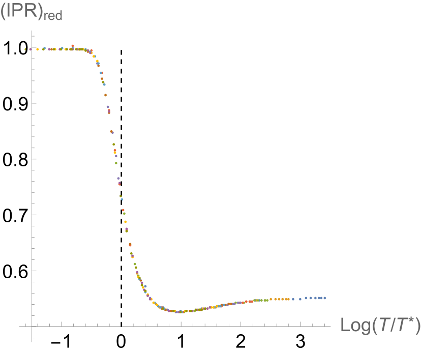
Figure 2: $(IPR)_{red}$ vs. Reduced Temperature. The curves shown in Fig. 1 can be cast into a reduced form with a single critical temperature, $k_{B}T^{*}=g^{2}/J$. The colored points correspond to the data in Fig. 1. The dashed line indicates the critical temperature.

We now turn our attention towards the exciton lineshape as a function of $T$ for various parametric ranges. To reiterate, the homogeneous lineshape is proportional to the RMS deviation of the exciton energy about its mean. For this, we compute

$$\sigma_{E}^{2}=\langle(E-\langle E\rangle)^{2}\rangle$$ (41)

directly from the positive-branched eigenvalues of Eq. 25 with the appropriate thermal weights. The results are shown in Fig. 3. As expected, the line width increases with increasing $T$ when the coupling to the lattice is sufficiently strong.

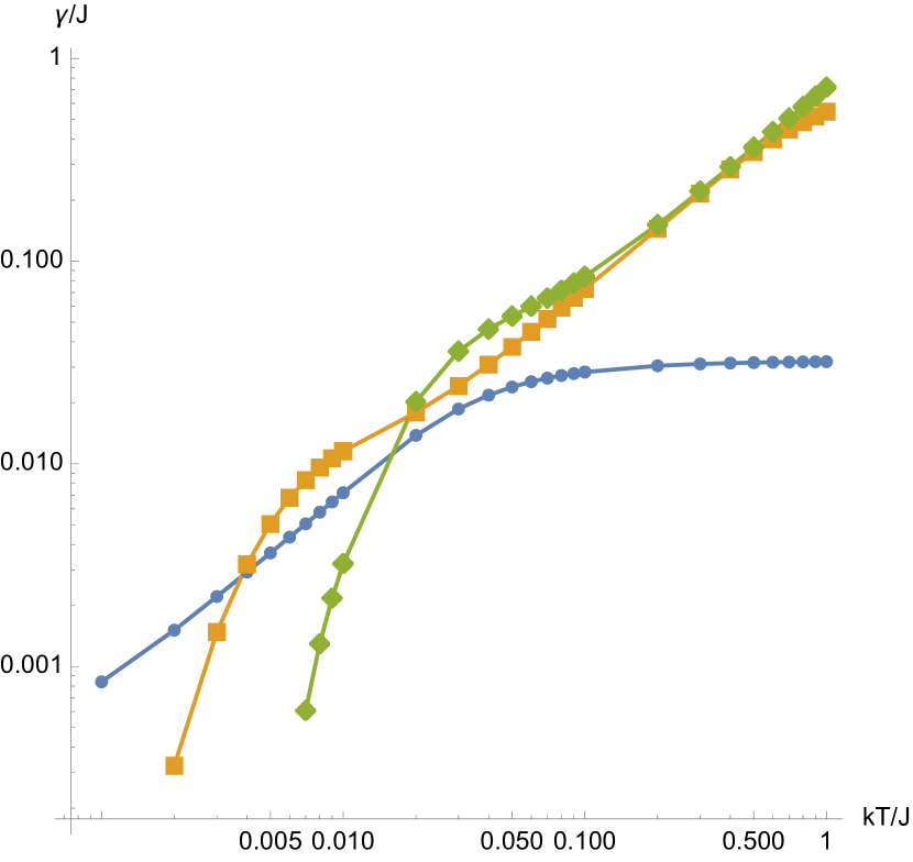
Figure 3: Exciton homogeneous linewidth $\gamma$ vs. Temperature at various coupling strengths. Blue: $g/J=0.1$ ; gold: $g/J=0.5$; green: $g/J=1$. Taking a typical coupling as $J=200meV$, these correspond to $T^{*}=23K$ (blue), $580K$ (gold) and $2321K$ (green), respectively.

For the case of weak coupling ($g/J\ll 1)$ the line width increases linearly with increasing temperature and eventually saturates at higher temperatures. The behaviour at strong coupling is dominated by quantum fluctuations at low temperature becoming linear before rolling over to a finite width. As in the reduced IPR curve in Fig. 2, the homogeneous line width curves can be cast in a reduced form by scaling with respect to the critical temperature as given in Fig. 4. In this case, the inflection in the numerical data occurs at $T=2T^{*}$.

The critical temperature clearly marks the boundary between the high and low-temperature limits of our model. As such, it is useful to put some in experimental numbers for the reorganization energy and the exciton hopping integrals. The reorganization energy for $J-$aggregate systems is typically on the order of 10-20 meV for organic systems. [12, 13, 14, 15, 16] This gives a critical temperature of 4200K (0.360 meV), which implies that most and if not all systems of interest are in the low-temperature limits of our model.

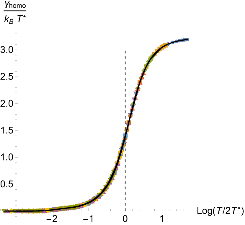
Figure 4: Homogeneous line width vs. temperature. The dashed line corresponds to the inflection point in the data at $T=2T^{*}$.

This is important since above $T^{*}$ it is unlikely that the assumption we made relating the lattice displacement and the soliton wave function in Eq. 18 is likely invalid since thermal noise in the lattice will strongly disrupt the smooth traveling waveform we have imposed on the system.

III Discussion

We present here a model for the Davydov soliton at finite temperature and use it to understand localization and energy fluctuations of excitons in conjugated polymers. However, the story of the finite temperature Davydov soliton reaches back a half-century within the peptide literature, starting with Davydov’s papers in the 1970’s. [6, 9] Simulations and theoretical treatments with various degrees of “quantum-ness” regarding the lattice phonons gave conflicting reports concerning whether or not solitons could actually exist in peptides at finite temperature. While we will not attempt a comprehensive review of the relevant literature here, we shall briefly give some high points of the debate. Lomdahl and Kerr used finite-temperature mixed quantum classical molecular dynamics to integrate Eq. 13 and 14 and concluded that random thermal motions prevent self-trapping from occurring at temperatures of interest for transport in real proteins.[17] On the other hand, Forner addressed the question of finite-temperature effects in the Davydov model in a series of papers in the 90’s and concluded that in peptides at least, Davydov-like solitons are stable up to about 310K.[18, 19] Similarly, Cruzeiro et al. performed quantum/classical MD simulations[20] on the model and generally agree with Forner’s results. Hamm and Edler reported the direct observation of self-trapped vibtational soliton states in the amide-I band of model peptide crystals and in $\alpha-$helices of proteins. [21, 22] Goj and Bittner used a fully atomistic MD approach with realistic hydrogen-bonding interactions for a polypeptide chain in water, treating the CO vibrational exciton quantum dynamics with surface hopping, concluded that stable solitons could not form in poly-peptide oligomer chains in a hydrogen-bonding solvent due to competition with solvent-solute hydrogen bonding that disrupted the chain. [23]. Similarly, quantum/classical simulations suggest that solitons remain stable even along thermal gradients and could be useful conduits for quantum transport in a wide range of physical systems ranging from resonant electronic energy transport in DNA chains to Joule heating in molecular wires.[24] The various forms of the model have been proposed recently to study non-linear dynamics in DNA helices. [25]. The model remains a test-bed for incorporating finite-temperature/lattice dynamics into a solvable quantum model.

In this paper, we add to this rich discussion by introducing the lattice fluctuations effect in a way such that STE and the phonon lattice are kept in a stationary state. The fact that the stability matrix has only real-valued eigenvalues implies that the excitations from $T=0K$ produce stable oscillations and do not produce instabilities that would otherwise grow exponentially. Consequently, the treatment is valid at low temperatures with regards to the critical temperature $T^{*}=g^{2}/J$ for the system. The analysis also predicts that the finite temperature properties of the Davydov model over all parameter ranges can be described with the context of a single set of reduced parameters. It would be of interest to apply the analysis to other polaron models, such as the Su-Schrieffer-Heeger model[26] which has direct bearing on topological soliton states [27], topological insulators, and one-dimensional optomechanical arrays.[28]

Appendix A Discussion of the STE excitation spectrum

We briefly discuss the properties of the anti-Hermitian matrix used to determine the fluctuations from the localized STE state. As shown above, by introducing fluctuations about the STE state, $\phi\to\phi_{o}+\delta\phi$ and reintroducing this into the NLSE one obtains

$${\bf T}\cdot{\bf y}=\hbar\omega{\bf y}$$ (42)

where $T$ is the anti-Hermitian matrix

$${\bf T}=\left[\begin{array}[]{cc}A&B\\ -B^{*}&-A\end{array}\right]$$ (45)

with

$$A =(-J\partial_{x}^{2}-2gn(x)-\hbar\mu)$$ (46)

$$B =-gn(x)$$ (47)

and

$${\bf y}=\left[\begin{array}[]{c}u(x)\\ v(x)\end{array}\right]$$ (50)

are the two-component eigenfunction solutions.

The fact that ${\bf T}$ is non-Hermitian implies that its eigenvalues may take complex values, which will imply that the resulting fluctuations will either grow or decay exponentially in time. The $2\times 2$ matrix ${\bf T}$ possesses important symmetries under $su(2)$ transformations, namely

$$\sigma_{1}\cdot{\bf T}\cdot\sigma_{1} =-{\bf T}^{*}$$ (51)

$$\sigma_{2}\cdot{\bf T}\cdot\sigma_{2} =-{\bf T}^{T}$$ (52)

$$\sigma_{3}\cdot{\bf T}\cdot\sigma_{3} ={\bf T}^{\dagger}.$$ (53)

using the usual definitions of the Pauli matrices. The last of these implies that ${\bf T}$ is pseudo-hermitian and consequently,

$$({\bf y}_{i},{\bf T}{\bf y}_{j})=({\bf T}{\bf y}_{i},{\bf y}_{j})$$

and $({\bf y}_{i},{\bf y}_{j})=({\bf y}_{j},{\bf y}_{i})^{*}$. This leads to

$$(\omega_{i}-\omega_{j}^{*})({\bf y}_{j},{\bf y}_{i})=0$$ (54)

which means that eigenfunctions with different eigenvalues must be orthogonal according to the inner product rule

$$({\bf y}_{i},{\bf y}_{j}) =\int dx{\bf y}_{i}^{\dagger}(x)\sigma_{3}{\bf y}_{j}(x)$$ (55)

$$=\int dx\left(u^{*}_{i}(x)u_{j}(x)-v^{*}_{i}(x)v_{j}(x)\right).$$ (56)

This preserves the bosonic nature of the Bogoliubov transformation used in defining the fluctuations.

Furthermore, it implies that

$$Im(\omega_{n})({\bf y}_{n},{\bf y}_{n})=0.$$ (57)

That is to say, if $\omega_{n}$ is complex, then the norm $||{\bf y}_{n}||^{2}=0$. Else, if $\omega_{n}$ is strictly real, $||{\bf y}_{n}||^{2}\neq 0$ and can arbitrarily be normalized to unity. Also, if ${\bf y}$ is an eigenfunction of ${\bf T}$ with corresponding eigenvalue $\omega$ , then ${\bf z}=\sigma_{1}{\bf y}$ is also an eigenfunction of ${\bf T}$, but with eigenvalue $-\omega$. Thus, all real eigenvalues are paired with $\pm\omega$ and their corresponding norms are non-zero with

$$||{\bf y}||^{2}=-||{\bf z}||^{2}.$$

For convenience, we take the branch with $+\omega_{n}>0$ to have eigenvectors ${\bf y}_{n}$ and the the branch with $\omega_{n}<0$ to have eigenvectors ${\bf z}_{n}$. We use the positive eigenvalue branch to construct the thermal properties of the STE state.

Data Availability:The data that supports the findings of this study are available within the article.

References

- [1] P W. Anderson. A mathematical model for the narrowing of spectral lines by exchange or motion. J. Phys. Soc. Jpn., 9(3):316–339, 1954.
- [2] Ryogo Kubo. Note on the stochastic theory of resonance absorption. J. Phys. Soc. Jpn., 9(6):935–944, 1954.
- [3] Ryogo Kubo. A stochastic theory of line shape, volume 15, pages 101–127. John Wiley & Sons, 1969.
- [4] Pascal Grégoire, Eleonora Vella, Matthew Dyson, Claudia M. Bazán, Richard Leonelli, Natalie Stingelin, Paul N. Stavrinou, Eric R. Bittner, and Carlos Silva. Excitonic coupling dominates the homogeneous photoluminescence excitation linewidth in semicrystalline polymeric semiconductors. Phys. Rev. B, 95:180201, May 2017.
- [5] Dylan H. Arias, Katherine W. Stone, Sebastiaan M. Vlaming, Brian J. Walker, Moungi G. Bawendi, Robert J. Silbey, Vladimir Bulović, and Keith A. Nelson. Thermally-limited exciton delocalization in superradiant molecular aggregates. The Journal of Physical Chemistry B, 117(16):4553–4559, 2013. PMID: 23199223.
- [6] A.S. Davydov. The theory of contraction of proteins under their excitation. Journal of Theoretical Biology, 38(3):559–569, 1973.
- [7] R Kubo. The fluctuation-dissipation theorem. Reports on Progress in Physics, 29(1):255–284, jan 1966.
- [8] Abraham Nitzan. Chemical Dynamics in Condensed Phases. Oxford University Press, Oxford, UK, 2006.
- [9] A.S. Davydov. Solitons and energy transfer along protein molecules. Journal of Theoretical Biology, 66(2):379–387, 1977.
- [10] Alwyn Scott. Davydov’s soliton. Physics Reports, 217(1):1–67, 1992.
- [11] NDEigenvalues, 2015. [Mathematica v.12.3.0].
- [12] Jean-Luc Brédas, David Beljonne, Veaceslav Coropceanu, and Jérôme Cornil. Charge-transfer and energy-transfer processes in -conjugated oligomers and polymers: A molecular picture. Chemical Reviews, 104(11):4971–5004, 2004. PMID: 15535639.
- [13] Frank C. Spano and Carlos Silva. H- and j-aggregate behavior in polymeric semiconductors. Annual Review of Physical Chemistry, 65(1):477–500, 2014. PMID: 24423378.
- [14] Frank C. Spano. Excitons in conjugated oligomer aggregates, films, and crystals. Annual Review of Physical Chemistry, 57(1):217–243, 2006. PMID: 16599810.
- [15] Jenny Clark, Jui-Fen Chang, Frank C. Spano, Richard H. Friend, and Carlos Silva. Determining exciton bandwidth and film microstructure in polythiophene films using linear absorption spectroscopy. Applied Physics Letters, 94(16):163306, 2009.
- [16] Alexei Cravcenco, Yi Yu, Fredrik Edhborg, Jonas F. Goebel, Zoltan Takacs, Yizhou Yang, Bo Albinsson, and Karl Börjesson. Exciton delocalization counteracts the energy gap: A new pathway toward nir-emissive dyes. Journal of the American Chemical Society, 143(45):19232–19239, 2021. PMID: 34748317.
- [17] P. S. Lomdahl and W. C. Kerr. Do davydov solitons exist at 300 k? Phys. Rev. Lett., 55:1235–1238, Sep 1985.
- [18] W Forner. Quantum and temperature effects on davydov soliton dynamics. II. the partial dressing state and comparisons between different methods. Journal of Physics: Condensed Matter, 5(7):803–822, feb 1993.
- [19] W Forner. Davydov soliton dynamics: temperature effects. Journal of Physics: Condensed Matter, 3(24):4333–4338, jun 1991.
- [20] L. Cruzeiro, J. Halding, P. L. Christiansen, O. Skovgaard, and A. C. Scott. Temperature effects on the davydov soliton. Phys. Rev. A, 37:880–887, Feb 1988.
- [21] J. Edler and P. Hamm. Self-trapping of the amide i band in a peptide model crystal. The Journal of Chemical Physics, 117(5):2415–2424, 2002.
- [22] Julian Edler, Rolf Pfister, Vincent Pouthier, Cyril Falvo, and Peter Hamm. Direct observation of self-trapped vibrational states in -helices. Physical Review Letters, 93:106405, 2004.
- [23] Anne Goj and Eric R. Bittner. Mixed quantum classical simulations of excitons in peptide helices. The Journal of Chemical Physics, 134(20):205103, 2011.
- [24] Eric R. Bittner, Anne M. Goj, and Irene Burghardt. Drift-diffusion of a localized quantum state along a thermal gradient in a model -helix. Chemical Physics, 370(1):137–142, 2010. Dynamics of molecular systems: From quantum to classical.
- [25] Dalibor Chevizovich, Davide Michieletto, Alain Mvogo, Farit Zakiryanov, and Slobodan Zdravković. A review on nonlinear dna physics. Royal Society open science, 7(11):200774–200774, 11 2020.
- [26] W. P. Su, J. R. Schrieffer, and A. J. Heeger. Solitons in polyacetylene. Phys. Rev. Lett., 42:1698–1701, Jun 1979.
- [27] Eric J. Meier, Fangzhao Alex An, and Bryce Gadway. Observation of the topological soliton state in the su–schrieffer–heeger model. Nature Communications, 7(1):13986, 2016.
- [28] Xun-Wei Xu, Yan-Jun Zhao, Hui Wang, Ai-Xi Chen, and Yu-Xi Liu. Generalized su-schrieffer-heeger model in one dimensional optomechanical arrays. Frontiers in Physics, 9, 2022.