Galactic chemical evolution of the solar neighborhood, solar twins and exoplanet indicators

Abstract

Galactic chemical evolution (GCE), solar analogues or twins, and peculiarities of the solar composition with respect to the twins are inextricably related. We examine GCE parameters from the literature and present newly derived values using a quadratic fit that gives zero for a Solar age (i.e., 4.6 Gyr). We show how the GCE parameters may be used not only to “correct” abundances to the solar age, but to predict relative elemental abundances as a function of age. We address the question of whether the solar abundances are depleted in refractories and enhanced in volatiles and find that the answer is sensitive to the selection of a representative standard. The best quality data sets do not support the notion that the Sun is depleted in refractories and enhanced in volatiles. A simple model allows us to estimate the amount of refractory-rich material missing from the Sun or alternately added to the average solar twin. The model gives between zero and 1.4 earth masses.

1 Introduction

Galactic chemical evolution (GCE) refers to the relation between the abundances of chemical elements and ages of the stars. Elemental abundances of the Sun and its twins are the keystone to galactic chemical evolution in the solar neighborhood–a volume defined by stars with mean distances of $\leq$ some 100 pc (Bedell et al., 2018). The elemental abundance is typically taken as the logarithmic ratio of an element to a reference element, which is usually hydrogen or iron: $[El/H]$ or $[El/Fe]$. The bracket notation indicates that the stellar ratio is relative to a standard. That standard is usually the Sun, although we explore the possibility of using some average of nearby solar-type stars.

In the small volume within some 100 pc of the Sun, secular changes due to stellar nucleosynthesis are modified by the diffusion of stars from the interior and exterior of the Galaxy (Manea et al., 2022). Possible stream remnants further complicate the picture (Matsuno et al., 2021), adding random or stochastic components to any overall smooth relation between mean abundance and age. Nevertheless a number of studies have described the behavior of $[El/Fe]$ with stellar age by a simple linear relation (cf. Bedell et al. (2018) and references below). We explore below the use of GCE parameters which give zero for a star of the solar age.

2 The data

The present work is entirely based on published results of five studies of stellar abundances and ages. Three of these, Bedell et al. (2018, henceforth, BD18) which includes data from Spina et al. (2018), Nissen et al. (2020, henceforth, NIS), and Liu et al. (2020, henceforth, LIU), give data for fewer than 100 stars. Two, Brewer et al. (2016, henceforth, BR) and Delgado Mena et al. (2017, 2019, henceforth, DM), have data for more than 1000 stars. Stellar ages have been taken directly from the cited references.

All five works use the method of precision differential abundances (PDAs, cf. Monroe et al. (2013). Abundance differences are based on ratios of abundances from line pairs for each spectrum (e.g., Fe i or Fe ii). Individual stellar properties do enter, as model atmospheres are used. However, the abundance differences are more accurate than individual abundances determined separately for each star, because uncertain factors such as oscillator strengths cancel.

Many papers relevant to PDAs, GCE, solar twins, and $T_{\rm c}$ correlations are not examined here. A sample list includes: Adibekyan et al. (2012), Adibekyan, et al. (2014), Adibekyan et al. (2015),Bensby et al. (2014), Battistini & Bensby (2016), Casali et al. (2020), Gonzalez et al. (2010), González Hernández et al. (2013), Ramirez et al. (2009), Ramírez et al. (2014a), Spina et al. (2016b), and Ramírez et al. (2014b). The latter reference is of interest because it lists all but one of the BD18 stars in a solar twin search. Additional references may be found in the exhaustive study of the solar twin problem by Yana Galarza et al. (2021).

We focus here on the BD18 work for two reasons. First, that study includes 30 elements from carbon to dysprosium, significantly more elements than in the other studies considered here. Second, we find the accuracy of the abundances is at least as good as the best of the others. The NIS survey has 13 elements, C-Ni, Sr and Y.   LIU has 17 elements C-Zn, Sr, Y, Zr, Ba-Dy. BR and DM are discussed below.

Tab. 1 will give some insight into the relative accuracy of the five studies. We give averages for the absolute value of the pairwise abundance differences for carbon, iron, aluminium, and silicon for stars in common. The mean and/or standard deviations of the differences in Tab.1 indicate that uncertainties range from the 0.01 dex level to somewhat more than 0.1 dex for some elements. The BD18 and NIS differences are the smallest.

Table 1: Abundance absolute magnitude differences for $[C/H],[Fe/H],[Al/H]$, and $[Si/H]$ from five studies

|BD18-BR|
	C	Fe	Al	Si
Mean	0.044	0.013	0.067	0.018
St. Dev.	0.032	0.009	0.138	0.023
No. Stars	15	15	15	15
|BD18-DM|
Mean		0.112	0.127	0.107
St. Dev.		0.053	0.093	0.020
No. Stars		8	8	8
|LIU-NIS|
Mean	0.073	0.040	0.080	0.025
St. Dev.	0.084	0.056	0.085	0.025
No. Stars	3	4	4	4
|BD18-NIS|
Mean	0.022	0.007	0.010	0.008
St. Dev.	0.011	0.005	0.009	0.005
No. Stars	22	22	22	22

• No carbon abundances in DM

• Carbon is an outlier for LIU-NIS in HD 4915 and is omitted

The BR and DM stellar samples are an order of magnitude more numerous (BR: 1615; DM: 1059) than BD18 and significantly more diverse in $T_{\rm eff}$, $\log(g)$, and composition. The BR stars have 15 elements, including nitrogen, missing from the other surveys. DM also has 15 elements: the refractories Mg - Ti and the intermediate volatiles Cu and Zn as well as Ba, Ce, Nd, and Eu.

The relation between stellar abundance and age for these surveys is complex. Plots of abundance versus age reveal “families” of stars defined by common spatial (thin or thick disk) or chemical (metal- or alpha-rich) properties (see Fig. 7 of DM). The BD18 data constitute a spatially and chemically more homogeneous group than the larger samples. Similar remarks apply to the NIS and LIU data.

3 Galactic Chemical Evolution–plots and parameters

Four of the five studies considered here, excepting BR, have obtained linear relations between $[El/Fe]$ and stellar age. We report values of GCE parameters for the BR stars based on a selected set of 160 stars described in Tab. 3 (see note to Col. 11).

The most common GCE parameters are the slope and intercept of a linear fit, or sometimes, a broken linear fit to a plots of $[El/Fe]$ vs. age such as in Fig. 1.

The elemental abundances of a star of a given age may considered as due to smooth, secular changes (GCE) and other, peculiar, causes such as accretion from a nearby supernova or the ingestion of an earthlike planet. These parameters may be used to compare the peculiar abundances of stars that are not due to the secular effect of GCE. If we want to compare the peculiar abundances of solar twins to the Sun, we must remove the differences due to GCE and obtain the abundances the star would have (had) if its age were 4.6 Gyr, the age of the Sun (Bonanno et al., 2002). We refer to these adjustments as “corrections”. Since the current linear fits do not give precisely zero corrections for 4.6 Gyr, we have explored two relations that do give precisely zero for the solar age. The first is a constrained linear (CL) relation with only one parameter. Its fits have significantly larger variances than the two-parameter unconstrained linear (UL) fits; it is therefore not useful. The second is a constrained quadratic (CQ), which like the UL fit has two free parameters.

The CQ fit, as well as the broken linear fits, allow for a change of slope with age. This can be of importance when attempting to make a correction for GCE, which depends on the slope of $[El/Fe]$ vs. age. The corrections add (or subtract) an amount from the $[El/Fe]$. For example, the BD18 GCE parameters, $m(age)$ and $b$ are used in

$$[El/Fe]_{\rm corrected}=[El/Fe]-[m(age)+b]$$ (1)

This linear correction does not allow for a change in slope $m$, so if the true slope does change the "correction" could be in the wrong direction for some age range!

The GCE plots of silicon and sodium are shown in Fig. 1. They represent the typical monotonic behavior of the abundances with age, and the occasional element for which the plot changes slope. A liberal uncertainty estimate for the points in the vertical direction is 0.022 dex, compatible with entry in Tab. 1, the mean of $|BD18-NIS|$ for carbon. The symbol in the upper left of the diagrams of Fig. 1 represents these abundance uncertainties. The age uncertainty is taken as 1.4 Gyr which is based on the standard deviation of independent age determinations of NIS and Spina et al. (2018). We present similar plots for all 30 elements and 79 stars of the BD18 study in the files PlotsofEloFe* at https://doi.org/10.5281/zenodo.6077735. The archive contains both PowerPoint (pptx) and pdf versions.

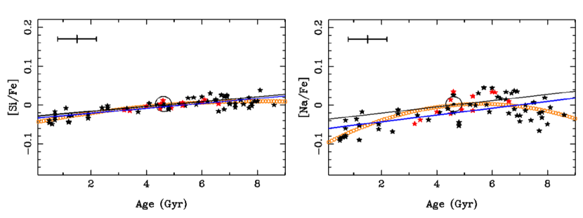
Figure 1: $[Si/Fe]$ and $[Na/Fe]$ vs. Age for 68 BD18 stars in Gyr. Blue: unconstrained linear (UL) fit; Black: constrained linear (CL) fit; Orange: constrained quadratic (CQ) fit. In these plots, the standard abundance is not that of the Sun but the average of the 12 BD18 twins of table 2. Selected “twins” are plotted as red stars. See text for further discussion.

The CQ parameters are derived by least squares fits to plots such as those of Fig. 1 and have the form

$$[El/Fe]=aa\cdot({\rm age}-4.6)+bb\cdot({\rm age}-4.6)^{2},$$ (2)

where $aa$ and $bb$ are constants for individual elements. Age is in units of Gyr. The constant $aa$ is the slope at age 4.6 Gyr.

Values of the variance ratios for the UL and CQ fits are remarkably close to unity for the BD18, NIS, and LIU samples. Most have values between 0.95 and 1.1, and none indicate a strong preference for the UL or CQ fits.

Plots similar to those of Fig. 1 were shown by da Silva et al. (2012) and Spina et al. (2016a). In the latter paper, three fitting techniques were employed: a simple linear and a broken linear fit as well as a hyperbolic fit (see their Fig. 1). Most of those hyperbolic fits are in qualitative agreement with those in PlotsofEloFe on zenodo: Na, Ca, Co, Ni, Cu, and Zn.

Table 2: Selected twins from BD18 stars and parameters

HD	HIP	Te (K)	$\log{g}$	$[Fe/H]$	age (Gyr)
13357	10175	5719	4.485	-0.028	3.2
16008	11915	5769	4.48	-0.067	3.4
36152	25670	5760	4.42	0.054	4.9
88072	49756	5789	4.435	0.023	4.5
115169	64713	5788	4.435	-0.043	5.3
124523	69645	5751	4.435	-0.026	5.3
138573	76114	5740	4.41	-0.024	6.6
146233	79672	5808	4.44	0.041	4.0
145927	79715	5816	4.38	-0.037	6.1
167060	89650	5851	4.415	-0.015	4.6
183658	95962	5805	4.38	0.029	6.0
200633	104045	5826	4.41	0.051	4.5
BD18 stars	averages	5785.	4.427	-0.0035	4.86

NIS (see their Fig. 4) has plots of $[El/Fe]$ for 12 elements vs. age similar to our Fig. 1. The color coding of these plots emphasizes their conclusion that the sample consists of two groups with distinct chemical history. The first group consists mostly of stars that are younger than the Sun, while stars of the second group are mostly older. This is consistent with the morphology of our plots of $[El/H]$ vs. atomic number, $Z$, which may be downloaded from zenodo. An examination of those plots of the BD18 data shows that most of the stars with positive overall shapes (POS) are younger than the Sun, while those with the V-shape are older (see Fig. 2).

The overall shapes of the NIS plots (see their Fig. 4) generally agree with our CQ fits, but not entirely. For example, the plot for $[Na/Fe]$ vs. age would support our negative curvature, except for high outliers which are unusually sodium rich: HD 1461, HD 66428, HD 111031, HD 134487, HD 134606, HD 169691, and HD 204313. These same stars lie below the mean of the $[O/Fe]$-plot; alternately, they are part of a separate population if broken GCE lines are adopted.

Figs. 4, 5, and 6 of LIU show $[El/Fe]$ vs age. We examined similar plots for their 68 “comparison” stars only, finding little convincing evidence of curvature, even for Na and Cu. Only 4 of the LIU stars were in the BD18 and NIS surveys.

The larger BR and DM samples are broader in the temperature-gravity spread. The DM stars are classified into populations. Most, 882, are thin disk. There are 108 thick disk, 60 high-$\alpha$, and 9 halo stars. This mixture causes apparent clustering in certain age ranges, often somewhat displaced from the general trend. In addition to DM’s published GCE parameters, we determined new UL ones based on severely limited samples (see Tab. 3 footnote to Col. 6). The 73 DM stars had all been classified as thin disk. BR does not explicitly classify its stars into populations, but notes the occurrence of $\alpha$-rich stars at sub-solar metalicities. Selection criterior for the BR stars are in the table footnotes to Cols. 11 and 12.

We made GCE fits to $[El/Fe]$ vs. age for the BR and DM samples. Without careful sample selection, the results show a considerable scatter due to the inclusion of populations that were purged in the BD18 sample. Different populations are readily seen in DM’s colorful plots of $[El/Fe]$ vs age (see Delgado Mena et al., 2019), Fig. 7.

Unlike the other four surveys, BR concentrated on the techniques and results of abundance determinations; GCE parameters were not obtained. We obtain them here for the limited sample of 160 BR stars.

In Tab.3 we compare published and newly computed slopes of the GCE relations from BD18, NIS, LIU and selections of stars from BR and DM. All newly derived parameters are from unweighted least squares fits. All of the stars are from the thin disk. We followed BD18 and excluded 11 of their 79 stars that are old, $\alpha$-rich or of the thick disk population. Thus the plots of Fig. 1 and in the zenodo archive are of the 68 thin disk stars. Similarly in Nissen (2015)’s study of 21 stars, they excluded 3 $\alpha$-enhanced stars from their GCE fits. In addition to the slopes from the 2015 paper, we present newly derived UL slopes based on the more recent Nissen et al. (2020) results, one determined using 71 stars excluding those with $[Fe/H]\geq 0.15$, (Col. 8), and 40 (Col. 9) stars also excluding those with $|[Fe/H]|\geq 0.15$. The Liu et al. (2020) figures are for the 68 “comparison stars” taken from that paper.

New UL coefficients for 73 DM stars are based on the criteria specified in 3, Col. 6. The age accuracy condition was adopted from DM and also applies to Cols. 5 and 6 of Tab. 3.

UL and CQ coefficients were derived in the present study from 160 stars of the BR study (Cols. 11 and 12). The 1615 BR stars were filtered as described in the supplement to Tab. 3.

The BR survey was the only one of the five discussed here to determine an abundance for the element nitrogen. This element is critical to the search for correlations of $[El/Fe]$ with $T_{\rm c}$, as there are only two other highly volatile elements that are spectroscopically available, carbon and oxygen. The $[N/Fe]$ ratio was included in the extensive examination of carbon isotopes and elemental nitrogen by Botelho et al. (2020). Fig. 5 of that study shows $[C/Fe]$ and $[N/Fe]$ vs. age; their broken-linear fit for nitrogen is in agreement with our CQ fit to the BR data–positive slope for the younger stars, and negative for the older.

Although the slopes of Tab. 3 differ numerically, they generally agree as summarized here:

1. For the lighter elements, the slopes are positive or small (e.g. Ca). Positive slopes indicate an increase in the $[El/Fe]$-ratio for the older stars.

2. Beyond the iron-group (3d) elements the slopes are mostly negative, indicating an increase in $[El/Fe]$ for the youngest stars.

3. The slope parameter for exceptions to items (1) and (2), such as for Ca or Cr are small.

4. The triplet of neutron-addition (nA) elements, Sr, Y, and Zr has very steep slopes in the BD18 data, and NIS data for Y.

5. The heaviest nA elements, from Ba to Dy all have negative slopes in the 68 BD18 stars. The DM slopes from Ba to Dy are mixed.

Table 3: GCE slopes for elements. CQ constants in Columns 2 and 3

1	2	3	4	5	6	7	8	9	10	11	12
el	aa	bb	BD18, m	Fig.7(DM)	DM(UL)	Nissen	Nissen	Nissen	Liu	Brew(CQ)	Brew(UL)
C	0.01481	-0.00227	0.0115	0.0187		0.0139	0.0162	0.0147	0.013	0.0091	0.0084
N										0.0093	0.0090
O	0.00849	0.00002	0.0088			0.0161	0.0201	0.0172	0.002	0.0141	0.0137
Na	0.00651	-0.00326	0.0086			0.0098	0.0064	0.0071	0.001	0.0161	0.0176
Mg	0.01027	-0.00054	0.0099	0.02059	0.0149	0.0089	0.0126	0.01	0.011	0.0145	0.0149
Al	0.01424	0.00007	0.0139	0.0126	0.0113	0.0167	0.0168	0.0163	0.033	0.0255	0.0272
Si	0.00578	-0.00086	0.0063	0.0075	0.0073	0.0006	0.0079	0.0065	0.000	0.0098	0.0104
S	0.00757	-0.00194	0.0098			0.0007			0.003
Ca	-0.00045	0.00105	-0.0011	0.00616	-0.0005	-0.0001	0.0026	0.0002	-0.002	-0.0016	-0.0016
Sc	0.00605	-0.00015	0.0059						0.024
Ti	0.00418	0.00053	0.0036	0.01136	0.0048	0.0063	0.0087	0.0062	0.007	0.0088	0.0079
V	0.00122	0.00010	0.0013						-0.013	0.0058	0.0043
Cr	-0.00131	0.00012	-0.0016			-0.0026	-0.0014	-0.0018	0.001	-0.0023	-0.0031
Mn	0.00075	-0.00235	0.0023						-0.012	0.0066	0.0072
Co	0.00628	-0.00176	0.0074						0.007
Ni	0.00575	-0.00218	0.0071			0.0048	0.0033	0.0041	0.007	0.0116	0.0124
Cu	0.01442	-0.00286	0.0149	0.00609	0.0112
Zn	0.00932	-0.00161	0.0102	0.01413	0.0121	0.0117			0.027
Sr	-0.02749	-0.00096	-0.0251	-0.01922	-0.0255		-0.0172	-0.0211
Y	-0.02581	-0.00106	-0.0238	-0.01658	-0.0223	-0.033	-0.0207	-0.0233	-0.007	-0.0159	-0.0149
Zr	-0.02359	-0.00088	-0.0219	-0.00787	-0.0165
Ba	-0.02898	0.00441	-0.0317	-0.01193	-0.0196
La	-0.02196	0.00155	-0.0227
Ce	-0.02007	0.00282	-0.0220	-0.00525	-0.0079		-0.0021
Pr	-0.01020	0.00028	-0.0103
Nd	-0.01800	0.00271	-0.0198	0.00767	-0.0021
Sm	-0.00727	0.00149	-0.0077
Eu	-0.00583	-0.00076	-0.0056	0.01058	0.0085
Gd	-0.00616	-0.00013	-0.0060
Dy	-0.00780	0.00234	-0.0073

• (Col. 1) Element

• (Col. 2) $aa$, CQ slope at 4.6 Gyr, Eq. 3, 68 stars, this work

• (Col. 3) $bb$, CQ constant, Eq. 3, 68 stars, this work

• (Col. 4) UL slope $m(t)$ taken directly from BD18 Table 3, 68 stars

• (Col. 5) DM GCE parameters a and b from Figure 7, for about 270 thin disk stars with age uncertainties $\leq$ 1.5 Gyr

• (Col. 6) 73 selected DM stars; age uncertainty $\leq 1.5$ Gyr, age < 9 Gyr, 5480 K < $T_{\rm eff}$< 6080 K, 4.24 < log($g$)< 4.64

• (Col. 7) Nissen et al. (2015) Table 6, 18 stars

• (Col. 8) Nissen et al. (2020), Vizier Cat., 71 stars

• (Col. 9) Same as 8, but -0.15 < [Fe/H] < 0.15, 40 stars

• (Col. 10) Liu, et al. (2020), Figs. 4, 5, & 6, 68 stars

• (Col. 11) Brewer, et al. (2016), 160 stars, CQ fit; age < 9.0 Gyr, 5400K < $T_{\rm eff}$< 6400K, 4.24 < log($g$), and -0.15 < $[Fe/H]$ < 0.15.

• (Col. 12) Brewer, et al. (2016), 160 stars, UL fit, same restrictions as CQ fit.

In Sec. 4 below, we consider the question of whether the abundance deviations from solar values are correlated with elemental condensation temperatures, $T_{\rm c}$ (Lodders, 2003). Many studies have looked for such correlations (see references in Sec. 2).

The chemical elements with stellar abundances have an obvious correlation of $[El/Fe]$ with GCE (Adibekyan, et al., 2014). Basically, the volatile elements carbon and oxygen are more abundant relative to iron, silicon and other refractories in older stars. Thus one should correct a star’s abundance for GCE prior to looking for a correlation with $T_{\rm c}$: The first part of Eq. 3 describes the UL fit, while the second gives tha CQ fit, where the correction vanishes for 4.6 Gyr.

$$[El/Fe]_{\rm corr} = [El/Fe]_{\rm obs}-[m*{\rm age}+b],{\rm or}$$ (3)

$$= [El/Fe]_{\rm obs}-[aa\cdot({\rm age}-4.6)+$$

$$bb\cdot({\rm age}-4.6)^{2}].$$

The constants $m$, $b$, $aa$, and $bb$ belong to each element.

But these GCE coefficients have additional meaning. They give the mean abundance for the sample as a function of age. A motion picture display may be seen in the iPoster from the 235th meeting of the American Astronomical Society that shows the average abundance patterns $[El/H]$ as a function of atomic number. Ten epochs are shown in steps of 1 Gyr based on the BD18 UL parameters of their Tab. 3. They clearly illustrate the transition from a positive overall slope (POS) in young stars to a V-shaped configuration in the oldest stars. Those two basic shapes are illustrated by the squares (and stars) in Fig. 2.

A dominant feature of these plots is the migration of the triplet Sr, Y, Zr from high values in young to low values in old stars. While Sr, Y, Zr move downward with age, the lighter refractories, Mg, Al, Si (black dots between Z = 11, Na, and Z = 16, S) move up slightly. This accounts for the ratio $[Y/Mg]$ used as a Galactic clock (da Silva et al., 2012; Magrini et al., 2021), but also shows that the behavior of these two elements is closely related to their neighbors in Z.

Most of the downward migration of the Sr, Y, Zr triplet takes place within 2 Gyr of the Sun’s age. This could be related to the “bi-modality” of s-process production discussed by Kamath et al. (2021), as well as the two populations discussed by NIS.

In the young stars, with POS-type slopes the elements Mg-Zn align nearly perpendicular to the overall slope. In the older stars, this line rotates slightly counter clockwise, nearly as a whole. In the oldest stars, the heaviest elements of this group, Cu and Zn, disconnect, and move upward. This is due primarily to eleven stars that were purged from the original BD18 list of 79 stars but are included in the file BD18stars_plots in the zenodo archive.

We now compare the differential abundances of individual stars with the mean values computed from the CQ GCE coefficients. Fig. 2 shows two examples–of relatively young (HIP 101905) and old (HIP 15527) stars. The star symbols represent the elemental differential abundances for individual stars. Ordinates (y-values) for the squares are given by Eq. 3; we show the $Z$-dependence of the GCE coefficients explicitly:

$$y(Z,{\rm age}) = <[El/Fe]>_{\rm ave}$$

$$= aa(Z)\cdot({\rm age}-4.6)+bb(Z)\cdot({\rm age}-4.6)^{2}$$

The young-star abundances display the expected pattern– POS, both observed (stars) and predicted (squares). The older star shows the typical V-shape, due to the strong drop for the intermediate s-process-dominated elements Sr, Y, and Zr.

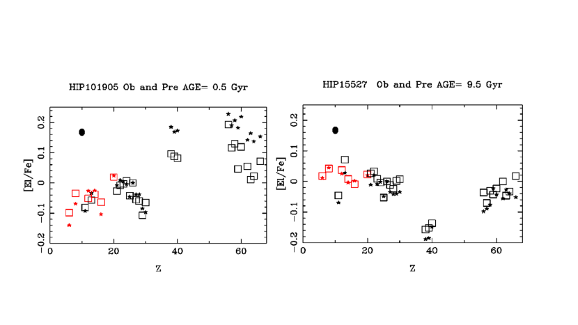
Figure 2: [El/Fe] vs. Z for 2 BD18 stars. Stars represent observed abundances while squares come from the CQ “average” fits. Alpha elements, C, O, Mg, Si, S, and Ca are shown in red. The black mark in the upper-left corner represents the uncertainty in $[El/Fe]$ for the star points, roughly 0.02 dex. The squares are computed directly from the CQ formula and do not have a similar uncertainty. See text for further discussion.

In Fig. 2 (left), the iron group (3d) elements follow the means (squares). The alpha elements scatter from the means (squares): C, O and S are about 0.04 dex low, while Mg, Si, and Ca are approximately fit. All of the neutron addition (nA) elements are significantly higher than the means.

Abundances in the older star fit the means more closely. Individual stars have their own usually small departures from the mean abundances for their age. Plots of this kind may be seen for all the BD18 stars in ObsandPrePlots in the zenodo archive. It will be seen that deviations from the average patterns are common, and occasionally as large as 0.1 dex.

4 Solar twins, condensation, and engulfment

Meléndez et al. (2009, henceforth, MEL09) showed that the Sun may not be the best chemical sample of its neighborhood. Their Fig. 3 is a good illustration, where logarithmic differential abundances–Sun minus twins–are plotted against condensation temperature, $T_{\rm c}$. This plot shows the highly volatile element C ($T_{\rm c}$ = 40K) with an excess of about 0.05 dex. The highly refractive Al ($T_{\rm c}$ = 1641K) has a depletion of about 0.03 dex. The extremes of about 0.08 dex, are comparable to the differences of Tab. 1, excepting BD18 and NIS. The corresponding slope, $-5\cdot 10^{-5}{\rm dex\ deg}^{-1}$ is similar in magnitude to those of (suspected and) confirmed planet host stars (see LIU Table 5, Column 2).

Numerous workers have sought an optimum sample of representative stars for the solar neighborhood. The topic was reviewed in detail by Yana Galarza et al. (2021), who discuss new criteria based on Gaia data, geochronology, and magnetic activity.

Our “twins” were selected with four parameters: $T_{\rm eff}$, $\log{(g)}$, $[Fe/H]$, and age, taken from the original papers (BD18, NIS, LIU, BR, and DM). A dozen stars were were chosen based on minimum Euclidian distances from the Sun in these parameters. Prior to calculating the distances, the variables were normalized to fall between -1 and +1. We selected the 12 stars with the smallest distances in hyperspace from the Sun for each of the surveys.

Average values of $[El/Fe]$ for the nA elements from carbon to zinc were obtained. This average of the logarithms is not the same as the logarithm of the (non-logarithmic) average (Bedell et al., 2018, see Eq. 1), but differs, typically, by one or two units in the third decimal, which is unimportant for our purposes. Note that averaging logs rather than taking an average of antilogs has the advantage of weakening the effect of outliers.

The BD18 twins are given in Tab. 2; the remaining sets are in Tab 4.

A number of very impressive abundance surveys are related to correlations of differential abundances with $T_{\rm c}$ as an indication of planetary engulfment (see references in Sec. 2).

The study by Spina et al. (2021) argues strongly that engulfment is the most likely explanation for many such correlations. However, they present an argument independent of $T_{\rm c}$, essentially based on the probability of abundance anomalies due to engulfment being more prominant in stars with higher effective temperatures with thinner convection zones.

Relative elemental abundance averages for each of the five surveys were plotted as a function of condensation temperature, $T_{\rm eff}$ (Lodders, 2003). Here, the relative abundances are for the Sun, with respect to the mean for the twins of Tab. 2 and Tab. 4. The average twin $[El/Fe]$ relative to the Sun and corrected with CQ for GCE we designati $[El/Fe]_{\rm twc}$, for "twin, corrected":

$$[El/Fe]_{\rm twc} = \frac{1}{12}\sum_{i=1}^{12}[El/H]_{\rm BD18}-[Fe/H]_{\rm BD18}$$ (5)

$$- \left(aa\cdot({\rm age}-4.6)+bb\cdot({\rm age}-4.6)^{2}\right)$$

The plots of Fig. 3 follow the orientation of MEL09, so that deficiencies of refractory elements in the Sun result in a downward slope with increasing $T_{\rm c}$.

Only elements from carbon to zinc were used. We excluded the neutron-addition (nA) elements from consideration in the search for $T_{\rm c}$ correlations for reasons noted by Meléndez et al. (2014), and adopted by Cowley et al. (2020) in their survey of the BD18 sample. Many examples may be seen in the plots of the BD18 abundances vs. $T_{\rm c}$, where the nA abundances scatter sometimes above (HIP 8507) and sometimes below (HIP 9349) the trends for the lighter elements (see TccorGIF1 in the zenodo archive). This is evidence that the neutron-addition elements have a distinct GCE from C-Zn, as argued by Meléndez et al. (2014).

The BD18 survey has abundances for 18 elements, from C to Zn, plus 12 nA elements not used here. BR has one such, element, Y, and 14 from C to Ni, including the ultravolatile, N, which is unavailable in the other two surveys. DM has only the intermediate volatiles Cu and Zn, and the refractories Mg - Fe.

Twins for BR, DM, NIS, and LIU in Tab. 4 are listed in order of their distance in hyperspace from the Sun. Thus, of the BR twins, HD 9407 is closer to the Sun in $T_{\rm eff}$, $log(g)$, $[Fe/H]$, and age than HD 157347.

Table 4: Twins from four PDA surveys; last row gives minimum and maximum ages in Gyr

BR(160*)	DM(73*)	NIS(71*)	LIU(68*)
HD	HD	HD	HD
9407	150437	2071	146233
157347	29137	1461	140538
152391	134987	4915	138004
203030	115585	361	68168
50692	90722	7134	10307
147750	33822	6204	190406
103828	109271	13724	106116
85689	134664	196390	219542
157338	147513	189625	141937
34411	76151	202628	159222
24496	155968	12264	4915
10307	189625	59967	217014
4.3–4.9	1.6–7.2	1.5–7	2.5–6.8

Figure 3: $[El/Fe]_{\rm twc\ or\ 68twc}$ = $[El/Fe]_{\rm Sun}-[El/Fe]_{\rm Average\,twins}$. vs. condensation temperature, $T_{\rm c}$. Filled circles are BD18 points; grey (blue online) points are volatiles C (40K), O (179K), Na (953K), S (655K), and Zn (723K) and Cu (1033K). Black filled circles are refractories. Error bars are the lengths of the standard deviations of BD18 minus NIS Left: GCE CQ corrections are used. Right: UL GCE corrections used. The straight lines are an unweighted least square fits. Note the different vertical scales, left and right.

Fig. 3 uses GCE-corrected abundances for 12 twins, by CQ (left) and 68 twins UL (right), numerical values for the latter are from BD18’s Tab.  3. Error bars are given for elements in common for BD18 and NIS surveys. The bar lengths are equal to the standard deviations of $[El/H]_{\rm BD18}-[El/H]_{\rm NIS}$ for the 11 non neutron-addition elements in common. S, Zn, Cu, and Mn (1158 K) were not determined in NIS.

Neither fit in Fig. 3 is significant The larger of the absolute value of the two tiny slopes is $-0.21\cdot 10^{-5}$ for the 12 twins (left). This “lack” of an indication of depletion of the solar refractories was sufficiently surprising that a calculation was made using all 68 stars from BD18 as twins. We again excluded 11 of their 79 stars. The resulting plot, Fig. 3 (right) supported the normality of the solar refractory abundances relative to these two sets of twins.

A further confirmation of the normality of solar refractories in BD18 are the abundances of a subset of 25 stars with ages within $\pm$ 1.5 Gyr of the Sun’s age. Because of their proximity to the Sun’s age, GCE corrections are small. Averages of $[El/Fe]$ are very small from a minimum of $-$0.026 for carbon and a maximum of +0.017 for calcium. Values for the refractory Ti (1573 K) and Al (1641 K) were respectively 0.013 and 0.006.

Scatter for the other surveys is larger than for BD18. If we combine the recent NIS and LIU into 26 points, unweighted linear fits (not shown) have slopes of $-1.39\times 10^{-5}{\rm dex\ deg}^{-1}$ (uncorrected for GCE), sig = 0.054, and $-0.95\times 10^{-5}{\rm dex\ deg}^{-1}$ (corrected), sig = 0.20, giving weak support to the depletion of solar refractories. An examination of 60 NIS stars with ages < 9 Gyr shows small depletion of all 10 elements from carbon to nickel. Depletions of refractories magnesium – nickel are all < 0.02 dex if GCE corrections are applied. The greatest depletion is for oxygen, -0.04 dex.

It is possible to relate the slopes of abundance vs $T_{\rm c}$ plots to an engulfed mass using the toy model of Cowley et al. (2021). The model gives the slope, $q$, of the $[El/H]$ vs. $T_{\rm c}$plot. Because $[El/H]=[El/Fe]-[Fe/H]$ there will be no difference in the slope of plots of $[El/H]$ and $[El/Fe]$ for constant $[Fe/H]$.

We assume solar abundances (Asplund et al., 2021) for the mass and composition of the convection zone (SCZ) as well as the composition of the mass ($q\times M_{\rm BE}$) added. Here, we take $M_{\rm SCZ}=0.025M_{\odot}$, having the Sun’s composition (Asplund et al., 2021). For negative slopes, the mass is added to the average solar twin and missing from the Sun.

The added mass is $q$ times the earth’s mass and has the earth’s composition (Wang et al., 2018). For other convection zone masses, the added mass must be adjusted accordingly–e.g. in a linear regime, doubling the $M_{\rm SCZ}$ would require doubling the added mass.

Quantitative values for the $q$ parameters and the corresponding slopes are given in Tab. 5. The coefficient of $10^{-5}$ is fortuitously nearly equal to $q$ because of the correlation of $M_{\rm BE}/M_{\rm SCZ}$ with $T_{\rm c}$.

Table 5: Slopes of $[El/H]$ for different values of $q$; last row gives minimum and maximum ages in Gyr

$q$	slope*105	$q$	slope*105
0.02	0.02	1.0	1.08
0.10	0.11	3.0	3.13
0.33	0.36	10.0	9.35
0.50	0.54	30.0	22.1

The negative slopes of the abundances vs. $T_{\rm c}$ indicate 0.21 to 1.4 $M_{\rm BE}$ was added to the average solar twin but is missing from the Sun. The tiny slopes of Fig. 3 corresponds to no refractive mass difference in the Sun and average twin.

5 Summary

We have examined precision differential abundances from five surveys. We obtained new GCE parameters from the BD18 set, using an algorithm that gives zero correction for stars with solar age. The new constrained quadratic (CQ) algorithm allows for curvature that is in agreement for a number of elements with previous studies and in particular supports the conclusion of NIS of two populations with different abundance patterns for stars younger and older than the Sun. For most elements, curvature described by our CQ fits was small; the overall agreement BD18 parameters is good.

Sets of twelve stars were chosen from each of five surveys of F, G, and K stars as solar analogues or “twins.” The choice was based on proximity in a hyperspace consisting of $T_{\rm eff}$, $\log{(g)}$, [Fe/H], and age. Additionally, we considered a subgroup of 68 BD18 stars as twins.

Similar parameters for the NIS, LIU, and the larger DM and BR were obtained. Results depend sensitively on the selection of subsets of stars from the samples. Abundances from each set were averaged, and plotted against condensation temperature. The peak-to-peak scatter is nearly 0.1 dex, In the case of the BD18 data, that scatter is about 0.025 dex. The BD18 data does not support the thesis that the Sun is depleted in refractory elements. Examination of several subsets of the data shows generally very small depletions of solar refractories but also depletions of oxygen.

Depletions of the refractories in the Sun are probably < 0.02 dex, but depend on the choise of comparison stars (twins).

A simple model of addition of bulk earth material to a solar convection zone connects the slopes of $[El/Fe]$ vs. $T_{\rm c}$ plots to the amount of ingested (or missing) refractory-rich material. We estimate the amount of ingested (or missing) material is between zero and 1.4 earth masses.

6 Data Availability

This work is based entirely on data that may be obtained from the CDS in Strasbourg France.

References

- Adibekyan et al. (2012) Adibekyan, V. Zh., Sousa, S. G., Santos, N. C., et al. 2012, A&A, 545, A32. doi:10.1051/0004-6361/201219401
- Adibekyan, et al. (2014) Adibekyan, V. Zh., González Hernández, J. I., Delgado Mena, E., et al. 2014, A&A, 564, L15 doi:10.1051/0004-6361/201423435
- Adibekyan et al. (2015) Adibekyan, V. Zh, Santos, N. C., Figueira, P., et al. 2015, A&A, 581, L2. doi:10.1051/0004-6361/201527059
- Asplund et al. (2021) Asplund, M., Amarsi, A. M., & Grevesse, N. 2021, A&A, 653, A141. doi:10.1051/0004-6361/202140445
- Battistini & Bensby (2015) Battistini, C. & Bensby, T. 2015, A&A, 577, A9. doi:10.1051/0004-6361/201425327
- Battistini & Bensby (2016) Battistini, C. & Bensby, T. 2016, A&A, 586, A49. doi:10.1051/0004-6361/201527385
- Bedell et al. (2018) Bedell, M., Bean, J. L., Meléndez, J., et al. 2018, ApJ, 865, 68. doi:10.3847/1538-4357/aad908 (BD18)
- Bensby et al. (2014) Bensby, T., Feltzing, S., & Oey, M. S. 2014, A&A, 562, A71. doi:10.1051/0004-6361/201322631
- Bonanno et al. (2002) Bonanno, A., Schlattl, H., & Paternò, L. 2002, A&A, 390, 1115B. doi:10.1051/0004-6361:20020749
- Botelho et al. (2020) Botelho, R. B., Milone, A. de C., Meléndez, J., et al. 2020, MNRAS, 499, 2196. doi:10.1093/mnras/staa2917
- Brewer et al. (2016) Brewer, J. M., Fischer, D. A., Valenti, J. A., et al. 2016, ApJS, 225, 32. doi:10.3847/0067-0049/225/2/32 (BR)
- Casali et al. (2020) Casali, G., Spina, L., Magrini, L., et al. 2020, A&A, 639, A127. doi:10.1051/0004-6361/202038055
- Cowley et al. (2020) Cowley, C. R., Bord, D. J., & Yüce, K. 2020, Research Notes of the American Astronomical Society, 4, 31. doi:10.3847/2515-5172/ab79a3
- Cowley et al. (2021) Cowley, C. R., Bord, D. J., & Yüce, K. 2021, AJ, 161, 142. doi:10.3847/1538-3881/abdf5d
- da Silva et al. (2012) da Silva, R., Porto de Mello, G. F., Milone, A. C., et al. 2012, A&A, 542, A84. doi:10.1051/0004-6361/201118751
- Delgado Mena et al. (2017) Delgado Mena, E., Tsantaki, M., Adibekyan, V. Zh., et al. 2017, VizieR Online Data Catalog, J/A+A/606/A94
- Delgado Mena et al. (2019) Delgado Mena, E., Moya, A., Adibekyan, V., et al. 2019, A&A, 624, A78. doi:10.1051/0004-6361/201834783 (DM)
- Gonzalez et al. (2010) Gonzalez, G., Carlson, M. K., & Tobin, R. W. 2010, MNRAS, 407, 314. doi:10.1111/j.1365-2966.2010.16900.x
- González Hernández et al. (2013) González Hernández, J. I., Delgado-Mena, E., Sousa, S. G., et al. 2013, A&A, 552, A6. doi:10.1051/0004-6361/201220165
- Kamath et al. (2021) Kamath, D., Van Winckel, H., Ventura, P., et al. 2021, arXiv:2112.04318.
- Liu et al. (2020) Liu, F., Yong, D., Asplund, M., et al. 2020, MNRAS, 495, 3961. doi:10.1093/mnras/staa1420 (LIU)
- Lodders (2003) Lodders, K. 2003, ApJ, 591, 1220. doi:10.1086/375492
- Magrini et al. (2021) Magrini, L., Vescovi, D., Casali, G., et al. 2021, A&A, 646, L2. doi:10.1051/0004-6361/202040115
- Manea et al. (2022) Manea, C., Hawkins, K. & Maas, Z. G. 2002, arXiv:2201.07809
- Matsuno et al. (2021) Matsuno, T., Hirai, Y., Tarumi, Y., et al. 2021, A&A, 650, A110. doi:10.1051/0004-6361/202040227
- Meléndez et al. (2009) Meléndez, J., Asplund, M., Gustafsson, B., et al. 2009, ApJ, 704, L66 doi:10.1088/0004-637X/704/1/L66 (MEL09)
- Meléndez et al. (2014) Meléndez, J., Ramírez, I., Karakas, A. I., et al. 2014, ApJ, 791, 14. doi:10.1088/0004-637X/791/1/14
- Monroe et al. (2013) Monroe, T. R., Meléndez, J., Ramírez, I., et al. 2013, ApJ, 774, L32. doi:10.1088/2041-8205/774/2/L32
- Nissen (2015) Nissen, P. E. 2015, A&A, 579, A52. doi:10.1051/0004-6361/201526269
- Nissen et al. (2020) Nissen, P. E., Christensen-Dalsgaard, J., Mosumgaard, J. R., et al. 2020, A&A, 640, A81. doi:10.1051/0004-6361/202038300 (NIS)
- Ramirez et al. (2009) Ramirez, I., Melendez, J. & Asplund, M. 2009, A&A, 508, L17. doi: 10.1051/0004-6361/200913038
- Ramírez et al. (2014a) Ramírez, I., Meléndez, J., & Asplund, M. 2014, A&A, 561, A7. doi:10.1051/0004-6361/201322558
- Ramírez et al. (2014b) Ramírez, I., Meléndez, J., Bean, J., et al. 2014, A&A, 572, A48. doi:10.1051/0004-6361/201424244
- Spina et al. (2016a) Spina, L., Meléndez, J., Karakas, A. I., et al. 2016, A&A, 593, A125. doi:10.1051/0004-6361/201628557
- Spina et al. (2016b) Spina, L., Meléndez, J., & Ramírez, I. 2016, A&A, 585, A152. doi:10.1051/0004-6361/201527429
- Spina et al. (2018) Spina, L., Melendez, J., Karakas, A. I., et al. 2018, VizieR Online Data Catalog, J/MNRAS/474/2580
- Spina et al. (2021) Spina, L., Sharma, P., Meléndez, J., et al. 2021, Nature Astronomy, 5, 1163. doi:10.1038/s41550-021-01451-8
- Wang et al. (2018) Wang, H. S., Lineweaver, C. H., & Ireland, T. R. 2018, Icarus, 299, 460. doi:10.1016/j.icarus.2017.08.024
- Wenger et al. (2000) Wenger, M., Ochsenbein, F., Egret, D., et al. 2000, A&AS, 143, 9. doi:10.1051/aas:2000332
- Yana Galarza et al. (2021) Yana Galarza, J., López-Valdivia, R., Lorenzo-Oliveira, D., et al. 2021, MNRAS, 504, 1873. doi:10.1093/mnras/stab987