Quantum information with top quarks in QCD
Abstract
Top quarks represent unique high-energy systems since their spin correlations can be measured, thus allowing to study fundamental aspects of quantum mechanics with qubits at high-energy colliders. We present here the general framework of the quantum state of a top-antitop () quark pair produced through quantum chromodynamics (QCD) in a high-energy collider. We argue that, in general, the total quantum state that can be probed in a collider is given in terms of the production spin density matrix, which necessarily gives rise to a mixed state. We compute the quantum state of a pair produced from the most elementary QCD processes, finding the presence of entanglement and CHSH violation in different regions of phase space. We show that any realistic hadronic production of a pair is a statistical mixture of these elementary QCD processes. We focus on the experimentally relevant cases of proton-proton and proton-antiproton collisions, performed at the LHC and the Tevatron, analyzing the dependence of the quantum state with the energy of the collisions. We provide experimental observables for entanglement and CHSH-violation signatures. At the LHC, these signatures are given by the measurement of a single observable, which in the case of entanglement represents the violation of a Cauchy-Schwarz inequality. We extend the validity of the quantum tomography protocol for the pair proposed in the literature to more general quantum states, and for any production mechanism. Finally, we argue that a CHSH violation measured in a collider is only a weak form of violation of Bell’s theorem, necessarily containing a number of loopholes.
1 Introduction
The Standard Model of particle physics is a relativistic quantum field theory, based on special relativity and quantum mechanics. Therefore, it allows to study fundamental properties of quantum mechanics in a genuinely relativistic environment, at the frontier of the known Physics. However, even though the Standard Model is inherently a quantum theory, observing basic quantum phenomena in a high-energy collider can become quite challenging due to the nature of the measurement process.
Some light on this problem can be shed by the field of quantum information, where most of the foundations of quantum mechanics find a direct application. There, a characteristic signature of quantumness is provided by the existence of correlations that cannot be accounted by a classical probability theory, arising due to the intrinsic wave nature of quantum mechanics. Here emerges the concept of entanglement [1, 2, 3], perhaps the most genuine feature of quantum mechanics. Entanglement plays a key role in quantum technologies like quantum computation, cryptography, metrology and teleportation [4, 5, 6, 7, 8, 9, 10]. In particular, the study of entanglement in high-energy setups is of fundamental interest since entanglement is expected to be critically affected by relativistic effects [11, 12, 13, 14, 15, 16]. A number of works have already addressed the role of entanglement in the context of high-energy physics [17, 18, 19, 20, 21, 22].
The simplest system which can exhibit entanglement is that formed by two qubits. In high-energy physics, an interesting realization of a two-qubit system is a pair of decaying spin-1/2 particles, since their spin correlations can be measured from the kinematical distribution of their decay products. The best candidate from the Standard Model to carry out such a measurement is the top quark, the most massive fundamental particle known to exist (), first discovered by the D0 and CDF collaborations at the Tevatron in the Fermilab in 1995 [23, 24]. Top quarks are typically produced in top-antitop () pairs which, due to their high mass, quickly decay well before any other process can affect their spin correlations. As a result, the spins of the pair are correlated with the kinematical distribution of the decay products, from where the original top spin quantum state can be reconstructed.
This feature has rendered top spin correlations a rich subject of study within high-energy physics [25, 26, 27, 28, 29, 30, 31, 32]. Indeed, spin correlations between pairs have already been measured by the D0 and CDF collaborations at the Tevatron with proton-antiproton () collisions [33, 34, 35], and by the ATLAS and CMS collaborations at the Large Hadron Collider (LHC) with proton-proton () collisions [36, 37, 38, 39, 40].
However, despite the extensive literature on the topic, only a very recent work has studied the entanglement between pairs [41]. Specifically, it was proposed that the entanglement of a pair can be detected at the LHC with high statistical significance using the current data recorded during Run 2. This would represent the first measurement ever of entanglement in a quark pair, and the highest-energy observation of entanglement so far. Entanglement has been also recently postulated as potentially sensitive to effects of New Physics beyond the Standard Model [42, 43]. An experimental protocol for the quantum tomography of a pair was also developed in Ref. [41], a canonical technique in quantum information but novel in the high-energy context. In parallel, some recent works have also addressed the possibility of measuring the violation of Bell inequalities with pairs [44, 45, 46], and also with pairs [47], which are massive spin-1 bosons. Even the measurement of such a basic quantum phenomenon as quantum interference can become non-trivial in a high-energy collider [48]. Apart from the intrinsic interest of studying foundational aspects of quantum mechanics at the frontier of the known Physics, all these works are paving the way to also use high-energy colliders for the study of quantum information theory. Due to their genuine relativistic behavior, the exotic character of the symmetries and interactions involved, as well as their fundamental nature, high-energy colliders are extremely attractive systems for these purposes.
Here, we provide the general formalism of the quantum state of a pair created through quantum chromodynamics (QCD) within a genuine quantum information approach. We discuss that, in general, the total quantum state that can be probed in a scattering experiment in a collider is given in terms of the so-called production spin density matrix [26], which is necessarily a mixed state.
For the specific case of a pair, we analyze in detail its quantum state for the most elementary QCD production processes: light quark-antiquark () or gluon-gluon () interactions. We extend the entanglement analysis of Ref. [41] to also include the violation of Bell inequalities, finding that both quantum phenomena emerge in certain regions of phase space for both and processes. Interestingly, the entanglement structure can be qualitatively understood in terms of basic conservation laws, without the need of knowledge of the particular details of QCD interactions.
We show that any realistic QCD mechanism of production can be seen as a statistical mixture of the previous building blocks. In particular, we focus on the case of and collisions, corresponding to the LHC and the Tevatron, respectively. We study the dependence of the quantum state on the energy of the collisions, extending the current phenomenological literature restricted to Run 2 of LHC [41, 44, 45, 46]. We find that, for sufficiently high energies, both types of collisions converge to the same state due to the dominance of processes.
In a high-energy collider, spin correlations are measured from the fit of the differential cross-section describing the angular distribution of the decay products [29, 49]. We propose realistic experimental observables for the characterization of the quantum state by integrating the signal in certain regions of phase space. At the LHC, it was shown that an entanglement signature can be obtained from the measurement of one single magnitude, proportional to the trace of the spin correlation matrix [41]. We prove in this work that the violation of Bell inequality can be also signaled from the measurement of just one parameter, the transverse spin correlations. Moreover, we carry out a study of the energy dependence of both signatures. Regarding the Tevatron, we find that an entanglement signature is provided by direct integration over the whole phase space.
Finally, we analyze in detail the conceptual significance of the experimental implementation of these techniques. We show explicitly that an entanglement measurement at the LHC represents the violation of a Cauchy-Schwarz inequality. In contrast, we do not expect a statistically significant observation of entanglement at the Tevatron. We argue that the quantum tomography protocol developed in Ref. [41] can be extended to more general quantum states, and to any production process. We discuss that, due to the nature of the detection process, only weak violations of Bell inequalities can be measured in a high-energy collider, since some loopholes, like those related to the free-will or to the detection efficiency, cannot be closed.
Remarkably, while the probability and the spin density matrix of each production process are computed by the high-energy theory, once both are given, we are simply left with a typical problem in quantum information involving the convex sum of two-qubit quantum states, where the usual techniques of the field can be applied. This important observation is translated into the article presentation, fully developed within a quantum information language, aimed at making it easily understandable by the physics community outside the high-energy field.
The paper is arranged as follows. Section 2 discusses in detail the general framework upon we build the results of this work, presenting the basic tools of two-qubit systems used throughout this work along with a general discussion about quantum states in colliders and relativistic particle-antiparticle production. Section 3 studies the quantum state in elementary QCD processes. Section 4 extends the previous results to more realistic processes occurring in actual colliders, analyzing in detail the energy dependence. Section 5 translates these ideas into relevant experimental observables. Section 6 provides some technical remarks about the experimental implementation of the discussed quantum information techniques. Finally, Section 7 summarizes the main conclusions, and discusses future perspectives. Technical details are given in the Appendices.
2 General formalism
2.1 Two-qubit systems
Quantum states are represented in general by a density matrix , a Hermitian non-negative operator with unit trace in a certain Hilbert space , . These conditions imply that the number of real parameters characterizing for is . Expectation values for observables are computed by taking the product trace, .
The most simple example of density matrix is provided by a qubit, that is, a two-level quantum system. The density matrix of a qubit takes the simple form
| (1) |
with the identity matrix and , , the usual Pauli matrices. A physical (i.e., non-negative) density matrix is described by Bloch vectors , with pure states given by unit vectors saturating the inequality. The coefficients completely determine the quantum state of the system. For a spin-1/2 particle, they represent the spin polarization, . An alternative description of can be provided in terms of angular momentum coherent states through the -representation (see Appendix A for a summary of its main properties):
| (2) |
where the angular momentum coherent states satisfy , and is the solid angle associated to the unit vector . The function is the qubit analogue of the celebrated Glauber-Sudarshan -function in quantum optics [50]. It is easily seen that can be always chosen as non-negative for any density matrix describing a qubit.
More intriguing quantum states arise in bipartite Hilbert spaces composed of subsystems . A quantum state is called separable iff it can be written as a convex sum of product states
| (3) |
with . An entangled state is defined as a non-separable state.
To illustrate this concept, we consider the case of a pair of qubits, whose density matrix can be decomposed as
| (4) |
Now, the quantum state of the system is determined by parameters , which for spin-1/2 particles are their spin polarizations , and their spin correlations .
An insightful way to understand entanglement for -qubit systems arises by considering the -representation
| (5) |
where . From Eq. (3), it is immediately seen that a state is separable iff it admits a non-negative -representation. This implies that the spin correlations for a separable state
| (6) |
are purely classical, described by a classical probability distribution. The same applies to the spin polarizations. Thus, in the language of the -function, entanglement is equivalent to a -function that necessarily presents negative values, a genuine distinctive signature of non-classicality and quantum behavior as well known from quantum optics [50].
In order to signal the presence of entanglement, several theoretical criteria can be used. Perhaps the most well-known one is the Peres-Horodecki criterion [51, 52], which simply states that if is separable, taking partial transpose with respect to the second subsystem
| (7) |
also yields a non-negative operator. Hence, a not positive semi-definite implies that is entangled. In two-qubit systems, the Peres-Horodecki criterion is also a necessary condition for entanglement.
A quantitative measurement of the entanglement of two qubits is provided by the concurrence [53]:
| (8) |
with the eigenvalues of the matrix ordered in decreasing magnitude, , and the complex conjugate of in the spin basis of . The concurrence is related to the entanglement of formation and satisfies , where a quantum state is entangled iff . Hence, implies that is maximally entangled.
The computation of these magnitudes requires full knowledge of the quantum state. This can be achieved by means of quantum tomography, a technique able to reconstruct a quantum state from the measurement of a selected set of observables. For the case of a single qubit, characterized by parameters, it is enough to measure the Bloch vector , which is the spin polarization for a spin-1/2 particle. For the case of two qubits, the quantum tomography is performed by measuring the parameters determining , which for spin-1/2 particles represent the spin polarizations and spin correlations, respectively. In actual experiments, an additional measurement is typically required to ensure the proper normalization of the density matrix [54]. Nevertheless, in order to detect entanglement, simpler criteria which require the measurement of just a few parameters can be formulated. Appendix B contains some general entanglement criteria specifically developed for quantum states and used throughout this work.
An even stronger requirement than entanglement is the violation of Bell-type inequalities [3]. No local hidden-variable model can give rise to it, implying a violation of local realism. The Clauser-Horner-Shimoni-Holt (CHSH) inequality [55] provides a particularly useful form of Bell inequality for systems:
| (9) |
where , are measurement settings in the Alice, Bob subsystems , and are their correlations. In the case of spin-1/2 particles, they can be interpreted as measurements of spin polarizations along certain directions defined by unit vectors , . Thus, Eq. (9) can be rewritten in vector notation as simply
| (10) |
with the same correlation matrix of Eq. (4). Any separable state of the form (3) satisfies Eq. (10). Hence, only entangled states can violate a CHSH inequality.
2.2 Quantum states in colliders
We now study how the physics in real colliders can be described in terms of quantum states. For illustrative purposes, we first address the simple non-relativistic scattering of an incident spinless particle with mass from a single fixed target, characterized by a potential (the interested reader is referred to Ref. [58] for the basics of scattering theory). The process is determined by the scattering matrix , whose elements in momentum representation are
| (12) |
where the -matrix satisfies the Lippmann-Schwinger equation , with the usual retarded free Green’s function, and is the kinetic energy. In the Dirac picture, the wave function of the scattered state resulting from an incident particle with well-defined momentum is
| (13) |
The scattering amplitude determines the differential cross-section characterizing the scattering to some momentum with the same energy,
| (14) |
being the solid angle associated to . Therefore, the differential cross-section is proportional to the probability of the process, given by the squared on-shell -matrix element connecting the initial to the final state.
The scattered state can be also rewritten as a density matrix:
| (15) | ||||
In a real collider, only momentum measurements of the scattered particle can be performed and thus, not all the information is needed to describe the quantum state in experiments. Moreover, scattering events along the beam direction are not typically measured. Therefore, the relevant quantum state that encodes all the information that can be probed in a collider results from projecting onto momentum states with the operators as
| (16) | ||||
where the factor in the denominator ensures proper normalization, . The quantum state described by the density matrix is thus mixed, resulting from the incoherent sum of momentum states with a probability proportional to the differential cross-section, where the total cross-section here plays an analogue role to the partition function in statistical mechanics. As a result, is written only in terms of differential cross-sections, the observables measured in actual colliders, computed in terms of -matrix elements. In this way, the expectation value of any momentum observable can be obtained from as
| (17) |
For a spin-half particle, things go along the same lines. By noticing that the spin of the scattered particle is not typically detected in a collider, we now project using with labeling spin indices, finding that the quantum state characterizing the scattering of an incident particle with momentum and spin is
| (18) |
where we have used . In the equation above, the partition function is defined to ensure normalization, and the production spin density matrix, in the following simply denoted as the -matrix [42], is defined as
| (19) |
The -matrix is not properly normalized, since its trace is proportional to the differential cross-section of the process,
| (20) | ||||
The proportionality factor can be chosen arbitrarily; for the present moment, we take directly proportional to the on-shell -matrix elements. Thus, the partition function becomes once more proportional to the total cross-section
| (21) |
As a Hermitian matrix, the most general form of the -matrix is similar to that of Eq. (1),
| (22) |
but with an extra parameter that determines the probability of the process, .
The proper spin density matrix with unit trace describing the quantum state for a scattering process along a fixed direction is obtained by normalization of ,
| (23) |
and whose spin polarization is given by . In terms of these quantum substates, the total quantum state of Eq. (2.2) can be written as simply
| (24) |
Hence, we can intuitively understand the total spin-momentum quantum state as the incoherent average in momentum of the spin quantum states describing the scattering along a fixed direction, weighted with the probability of that scattering process (proportional to the differential cross-section). The total cross-section plays once more the role of the partition function.
Finally, we note that in a collider the initial state is typically unpolarized since spin degrees of freedom cannot be controlled. Thus, the real quantum state describing the experiment after many events results from the averaged -matrix
| (25) |
In summary, the quantum state describing the scattered particles in a collider is a mixed state because of two fundamentally different reasons, related to the control over the degrees of freedom. (i) Regarding orbital variables: Momentum distributions of the scattered particles are the only measurable observables in colliders, given in terms of differential cross-sections. Thus, even if the scattered state is pure, one can only access to the diagonal part in momentum, which motivates the use of a reduced mixed density matrix. (ii) Regarding discrete variables: Internal degrees of freedom of the initial state cannot be typically controlled and one has to average uniformly over them. This average over all possible initial states after many scattering events results in an incoherent mixture that is described by a density matrix.
2.3 Relativistic particle-antiparticle pair production
We now switch to the actual case of high-energy colliders, whose physics is described by relativistic quantum field theories within the framework of the Standard Model. The Standard Model is composed of fundamental spin-1/2 particles (and their corresponding antiparticles) which interact through the mediation of gauge bosons of spin-1. These interactions can be either strong (mediated by massless gluons ), weak (mediated by the massive bosons), or electromagnetic (mediated by the photon ), corresponding to a Yang-Mills theory , respectively. Electromagnetic and weak interactions are both unified within the framework of electroweak theory, while strong interactions are described by quantum chromodynamics. The remaining particle of the Standard Model, the Higgs boson, has spin-0, and is the responsible for the occurrence of mass in massive particles.
A natural Standard Model candidate for an entangled two-qubit system is a particle-antiparticle (denoted generically as ) pair produced from some initial state :
| (26) |
In the following, we restrict to the case where is a Standard Model fermion of mass , although the formalism can be easily generalized to the case where is some massless spin-1 gauge boson like the photon. Among the Standard Model fermions, we can distinguish between quarks and leptons, where the latter do not interact through QCD since they do not have color degrees of freedom. Typically, the components of the initial state annihilate themselves through gauge interactions, giving rise to the pair. In the process, total energy and momentum are conserved.
The kinematics of a pair is determined in the center-of-mass (c.m.) frame by the invariant mass and the direction of flight of the particle . In this frame, the particle/antiparticle four-momenta read , with , and satisfy the Lorentz-invariant dispersion relation
| (27) |
where in the following we work in natural units .
The invariant mass is the c.m. energy of the pair, defined from the usual invariant Mandelstam variables as
| (28) |
In the c.m. frame, , where the momentum is related to the particle velocity by , so
| (29) |
Hence, threshold production () is at the minimum energy possible for a pair, , as naturally expected.
With respect to the quantum state of the pair, mutatis mutandis, we define again an -matrix in terms of the on-shell relativistic -matrix elements as
| (30) |
with labeling the initial state of the system and
| (31) |
where the first/second subspace correspond to the particle/antiparticle, respectively. The spins of the particles are computed in their respective rest frames, where they are well defined. Once more, if internal degrees of freedom of the initial state cannot be controlled (like spin or color), one uses the averaged -matrix
| (32) |
with the number of internal degrees of freedom of . In analogy to Eq. (2.2), the resulting quantum state is
| (33) | ||||
with the partition function proportional once more to the total cross-section
| (34) |
The -matrix characterizes the quantum state of any pair produced in a relativistic process, which is a mixed state by the very same reasons as in the non-relativistic case. It takes the general form
| (35) | ||||
in a similar fashion to Eq. (4), but once more with an extra coefficient proportional to the c.m. differential cross-section.
The actual spin density matrix is obtained from the normalization of :
| (36) |
As a result, the spin polarizations and spin correlations of the pair are
| (37) |
In terms of these quantum states, one can retrieve the relativistic version of Eq. (24),
| (38) | ||||
3 Production of in elementary QCD processes
A particularly interesting example of particle-antiparticle pair is provided by a top-antitop quark pair, which will be the subject of study throughout the rest of the work. Specifically, we restrict to the production of pairs through QCD processes, although the concepts and techniques developed here can be straightforwardly extended to other types of interaction and/or particle-antiparticle pairs. For the theoretical computations, we employ leading-order (LO) QCD perturbation theory, since it provides analytical results and a clear picture of the underlying physics. Higher-order corrections are known to be small and do not change the main results [29, 41, 44, 45, 42].
At LO QCD, only two initial states can produce a pair: a light quark-antiquark () or a gluon () pair,
| (39) | ||||
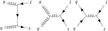
Representative Feynman diagrams for these processes in the Standard Model are depicted in Fig. 1.
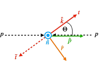
Each initial state creates a pair in a spin quantum state described by the production spin density matrix , where the spin and color degrees of freedom of the initial state have already been averaged, is the invariant mass of the pair, and is the flight direction of the top quark. For the characterization of the -matrix, an orthonormal basis needs to be fixed in order to compute the corresponding spin polarizations and correlations. The most common choice is the helicity basis [31], defined in the c.m. frame as , with , , where is a unitary vector along the direction of the initial state and is the production angle of the top quark with respect to the beam, . We note here that, due to momentum conservation, the c.m. frame of the initial state is the same as that of the pair.
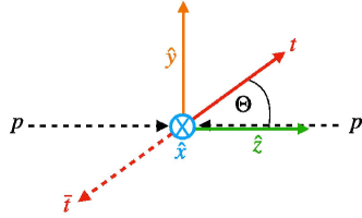
The advantage of the helicity basis is that, although the relativistic spins are only well-defined in their respective rest frames, those are equivalent to the c.m. frame via a Lorentz transformation along the top direction, which does not change the orientation of the helicity basis. A schematic representation of this basis is provided in Fig. 2.
The production spin density matrix in the helicity basis is only a function of (or, equivalently, of ) and . Specifically, in the Standard Model, the correlation matrix is symmetric and . Furthermore, at LO, the pair is unpolarized, , and, in QCD production, their spins along the -axis are uncorrelated with respect to the remaining directions, [39]. Therefore, is characterized at LO QCD by only parameters in the helicity basis: . The values of those coefficients can be computed analytically and are well known [28, 30, 31]. Here, we fix the normalization of such that the c.m. differential cross-section for production from an initial state is [28]
| (40) |
with the strong coupling constant characterizing the strength of QCD interactions.
 |
 |
The actual spin density matrices are computed from the normalization of . As a result of the above considerations, at LO is unpolarized, its correlation matrix is symmetric, and it is already diagonal in the direction. These last two properties imply that the correlation matrix can be diagonalized by an appropriated rotation in the plane, with eigenvalues ,
| (41) |
and orthonormal eigenvectors . We will refer to this orthonormal basis as the diagonal basis.
Regarding entanglement, since in all phase space and for both initial states [see Eqs. (45), (3.2)], we find that the Peres-Horodecki criterion is equivalent to (see Appendix B), where
| (42) | ||||
We note that this definition differs from that of Ref. [41] by a factor , so the concurrence is directly equal to for entangled states:
| (43) |
Previous approaches in high-energy physics based on the entanglement entropy [59, 60, 21] are not useful here since they are only valid for pure states. We recall that the entanglement of the quantum state is Lorentz invariant because it has well-defined momentum [11, 12].
Regarding the violation of the CHSH inequality, from Eq. (2.1) it is immediately seen in the diagonal basis to be equivalent to
| (44) | ||||
3.1 processes
For processes, the coefficients of the -matrix in the helicity basis are
| (45) | ||||
The resulting quantum state is entangled in the bulk of phase space as 111We note that the result for in Ref. [41] contained a typo, and a factor was missing.
| (46) |
The above inequality is saturated only at threshold () or for forward production (). In both limits, the spins are aligned along the beam axis in a maximally correlated but separable mixed state:
| (47) | ||||
where are the spin eigenstates along the direction . This spin alignment at threshold is a consequence of spin conservation, since the pair is produced from the initial state via gluon exchange (see Fig. 1), which is a massless spin-1 boson.
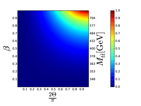
Hence, for low production angles or close to threshold, the degree of entanglement is expected to be small, as can seen in left Fig. 3, where the concurrence of is represented.
In the opposite limit of high transverse momentum (i.e., high energies and production angles close to ), the pair is in a spin-triplet pure state,
| (48) | ||||
This state is maximally entangled, , as seen in upper right corner of left Fig. 3.
With respect to the CHSH inequality, it is also violated by production processes in the bulk of phase space. This is seen in the diagonal basis, where
| (49) |
This basis is often called the off-diagonal basis [61] in the literature of processes, and is commonly used because the spins along the direction are perfectly correlated. Because of this,
| (50) |
Therefore, remarkably, entanglement and CHSH violation are equivalent conditions for processes.
3.2 processes
For processes, the coefficients of the -matrix in the helicity basis are
| (51) |
The resulting quantum state is entangled iff , where
| (52) |
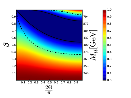
The second line implies that is not entangled for , so there are finite regions of separability in phase space, in contrast to the case. In particular, two regions of entanglement can be distinguished: one close to threshold, and another one for high , delimited by the lower and upper critical boundaries :
| (53) |
These features can be observed in right Fig. 3, where the concurrence of is represented, with the black solid lines signaling the critical boundaries between entanglement and separability.
The strong entanglement signature close to threshold results from the fact that the spin polarizations of the initial state are allowed to align in different directions. Due to angular momentum conservation, these features produce at threshold a pair in a spin singlet
| (54) | ||||
which is maximally entangled.
In the opposite limit of high , gluon fusion produces the same maximally entangled triplet state as processes, Eq. (48). The reason behind this similarity is that for high energies the orbital angular momentum contribution dominates over the spin contribution.
With respect to the violation of the CHSH inequality, the eigenvalues of the correlation matrix are
|
|
(55) |
As a result, an explicit analytical computation of the critical boundaries of the regions where the CHSH inequality is violated becomes much more cumbersome; even in the relatively simple case of , the critical values are obtained from the zeros of fourth order polynomials in , finding , and . The numerically computed boundaries are represented by black dashed lines in right Fig. 3. As expected, the regions where CHSH inequality is violated are within entangled regions of phase space, .
An important conclusion is that the entanglement structure of production can be mostly understood from basic laws of angular momentum conservation between the initial and final state, without the need to invoke technical details of the specific form of QCD interactions.
4 Production of in realistic QCD processes
Because of color confinement, quarks and gluons are not free particles and cannot be found isolated in nature. Instead, they are forming hadrons, which are bound states of quarks through QCD interactions. As a result, we can understand hadrons as a sea of quarks and gluons, which within this context are indistinctively denoted as partons [62, 63]. Quantitatively, the composition of a hadron is modeled by its so-called parton distribution function (PDF), which determines the participation of each parton in a particular QCD process at a certain energy scale. Due to its non-perturbative character, PDF distributions are typically computed by fitting experimental data (see Appendix C for more technical details about PDF). Here, we focus on production from two main types of hadron processes which are of high relevance for experiments: proton-proton collisions, as in the LHC, and proton-antiproton collisions, as in the Tevatron.
The above considerations modify the results of the previous section as following. For given energy and top direction in the c.m. frame, the -matrix describing the pair resulting from a hadronic process is computed in terms of each partonic matrix as
| (56) |
The function is the so-called luminosity function [28], and is computed in terms of the PDF describing the colliding hadrons. The luminosity function can be regarded as the probability distribution of occurrence of each initial state in the total hadronic process for a given , depending also on the hadron c.m. energy [see Eq. (134)]. We note that the c.m. frame of the colliding hadrons is not the same as the parton c.m. frame. However, at LO the direction of the parton initial state in its c.m. frame is to a very good approximation that of the initial hadron beam, so one can take safely along the hadron beam in Fig. 2, which is the one whose direction is controlled in a collider [29].
With the help of the luminosities and the -matrix, the differential cross-section characterizing production from a given hadronic process is computed as
| (57) | ||||
where the partonic differential cross-sections are those of Eq. (40). Thus, the differential cross-section per unit solid angle and per unit c.m. energy is just the sum of the partonic differential cross-sections from an initial state , multiplied by the probability distribution of producing each initial state with energy .
\stackinsetl18ptt12pt(a)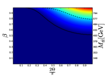
|
\stackinsetl18ptt12pt(b)
|
\stackinsetl18ptt12pt(c)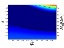
|
\stackinsetl18ptt12pt(d)
|
\stackinsetl18ptt12pt(e)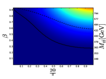
|
\stackinsetl18ptt12pt(f)
|
\stackinsetl18ptt12pt(g)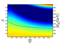
|
\stackinsetl18ptt12pt(h)
|
\stackinsetl18ptt12pt(i)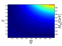
|
\stackinsetl18ptt12pt(j)
|
\stackinsetl18ptt12pt(k)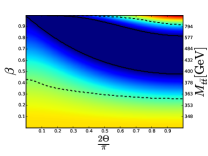
|
\stackinsetl18ptt12pt(l)
|
Regarding the actual spin quantum state, since , then
| (58) |
Similar expressions can be written for the spin polarizations and spin correlations of in terms of their partonic counterparts, computed from Eqs. (45), (3.2). The weights are obtained from the luminosities as
| (59) |
and represent the probability of production of each individual partonic quantum state , satisfying . They can be simply understood as the probability of occurrence of the initial state , , multiplied by the probability of producing a pair from , proportional to the differential cross-section, in turn proportional to the coefficient .
We stress that the nature of the specific hadron collision only enters in the calculations through the probabilities , which are PDF dependent. Hence, the LO QCD and processes are the building blocks of any realistic hadronic production process, whose role is reduced to change the amount of mixing between them. From a more general perspective, we can regard the production spin density matrices and the luminosities as inputs from the theory of high-energy physics, from which we can compute the physical spin density matrices and the probabilities . Once done, we are simply left with a typical problem in quantum information involving the convex sum of two-qubit states, where the usual techniques of the field can be applied.
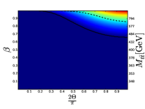
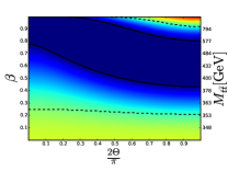
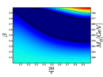
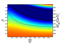
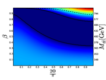
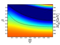
In order to understand better how the mixture between and channels affects the quantum state , we first use a toy model where both partonic probabilities are constant, . We gradually introduce processes in a pure reaction in upper row of Fig. 4. For a small amount of processes, the effect of mixing is reduced to shrink the entangled region towards the high region. By further increasing the amount of processes, at some point entangled states also emerge at threshold. We can actually compute from Eq. (42) the critical value at which entanglement appears, since
| (60) |
For , , so
| (61) |
Hence, in order to have entanglement close to threshold, we need at least of the pairs to be produced through gluon fusion. Regarding the violation of the CHSH inequality, the corresponding critical value is computed by switching to the off-diagonal basis where both correlation matrices are diagonal ( at threshold is a spin singlet, invariant under rotations). This gives
| (62) |
from where we find
| (63) |
Once this simple model is understood, we switch to real hadron processes. We analyze production from collisions for different c.m. energies in central row of Fig. 4. By direct comparison with upper row, we observe that for low c.m. energies processes dominate. However, the amount of processes increases with the c.m. energy, eventually dominating the production mechanism. A similar calculation is shown in the lower row of Fig. 4 for collisions where, although contributions are stronger at low energies, dominance is again recovered for sufficiently high c.m. energies, and both types of collisions converge to a similar quantum state.
 |
 |
We can further quantify the amount of mixing of and processes in the total production by computing the relative contribution of each channel to the total cross-section from Eq. (57):
| (64) |
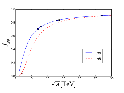
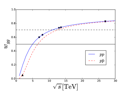
where we stress that the maximum invariant mass achievable by the pair is precisely the c.m. energy of the hadron pair, . The fraction of processes for both and collisions is represented in left Fig. 5, where its predicted increase with the c.m. energy indicated by the entanglement analysis is clearly observed, as well as the stronger contribution of processes for collisions with respect to at low energies. At high energies, both hadronic processes converge to the same gluon fraction . This analysis suggests that entanglement measurements can be also used to understand the underlying structure of a certain high-energy process without direct knowledge of it.
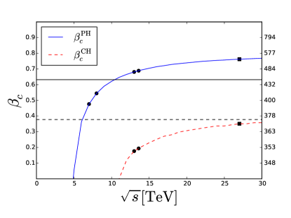
A related plot is that of right Fig. 5, in which the threshold values of the gluon probability are represented (there is no angular dependence at threshold). We observe that entanglement [] can be achieved in collisions for small c.m. energies , below current LHC energies. In particular, the relevant experimental values [36, 37, 38], [39, 40] and [64] are marked by circles, corresponding to the c.m. energies of Run 1, Run 2 and the ongoing Run 3 of the LHC, respectively. The expected value for a possible upgrade of the LHC is [65], marked by a square. In addition, the c.m. energy for collisions in the Future Circular Collider (FCC), [66], is represented explicitly in Fig. 4h. With respect to CHSH violation [], we observe that we need larger energies , with Run 2 and Run 3 only slightly above this limit. For collisions, even threshold entanglement cannot be observed since the c.m. energies required are well above the maximum energy achieved at the Tevatron, [33, 34, 35], marked by a triangle.
From these plots, we conclude that the Tevatron and the LHC provide experimental realizations to a very good approximation of the two main paradigms of production through QCD, and reactions.
5 Experimental observables
5.1 Experimental motivation
How are all these spin magnitudes translated into actual observables that can be measured in high-energy colliders? This is where the unique properties of the top quark enter in place. As explained in the Introduction, the top quark is the most massive particle of the Standard Model. This property makes that even its large width is still narrow when compared to its mass . In turn, this large width results in a very short lifetime . This implies that a pair decays so fast that any other process, such as hadronisation (with a time scale ) or spin decorrelation (with a time scale ), cannot affect their spin quantum state, whose information is directly translated into the properties of the decay products. This is what makes the top quark so special, as any other quark hadronizes before decaying, losing its spin information in the process. On the other hand, if the top quark did not decay, its spin state could not be extracted because detectors only measure the momentum of the arriving particles.
Quantitatively, we describe the decay of a top quark to some final state in terms of a decay spin density matrix, defined in the top rest frame as
| (65) |
where is the top state with zero momentum and spin , is the final state after the decay, and is here the on-shell -matrix determining the amplitude of the decay process. A similar decay spin density matrix can be defined for the decay of the antitop quark to a final state .
The idea is to describe the production and decay of a pair using the production and decay spin density matrices. Specifically, we consider a pair with fixed c.m. energy and momentum produced from a hadron collision, whose quantum state is specified by the matrix . In the so-called narrow-width approximation, valid since [26], the differential cross-section characterizing the decay of a pair to two final states is proportional to [29, 49]
| (66) |
Thus, the information about the quantum state of the pair, encoded in , is contained in the cross-section characterizing the decay products of the final states .
We can retrieve this information from final states including a lepton , which can be either an electron or a muon, . Specifically, we consider the electroweak leptonic decay of both the top and the antitop quark:
| (67) | ||||
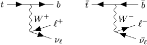
where , with the antilepton and its associated neutrino, and its conjugate, . A diagrammatic representation of the top/antitop decay is provided in Fig. 6.
The expression for the decay spin density matrices vastly simplifies if we integrate out all the degrees of freedom of the final states except for the lepton directions. In that case, due to the rotational invariance in the top (antitop) rest frames, the resulting decay spin density matrices can only be of the form [31]
| (68) |
being the antilepton (lepton) directions in each one of the parent top (antitop) rest frames, and the so-called spin analyzing powers of the leptons.
As a result, the cross-section characterizing the angular distribution reads
| (69) |
where , are the solid angles associated to , . The differential elements arise because we are considering the decay of a pair with fixed energy and direction. The total angular differential cross-section describing the leptons arising from the decay is then obtained by integration over all possible top directions and c.m. energies:
| (70) |
This implies that the normalized angular differential cross-section characterizing the dileptonic decay is
| (71) |
where the vectors and the matrix are the integrated values of the top/antitop spin polarizations and the spin correlation matrix, respectively. Therefore, we can measure all the integrated spin information of a pair by fitting the angular distribution of the leptonic decay products.
In particular, from the kinematic reconstruction of each event, the momenta of the and pairs can be determined. By defining the polar angle with respect to a certain direction given by the unit vector , , and after integrating over the azimuthal angles, we find that the spin polarizations can be easily obtained from a linear fit of the angular distributions for each individual lepton as
| (72) |
The spin correlations for a pair of directions can be measured from the distribution of the product , given by integration of Eq. (71):
| (73) |
Another measurable magnitude of interest is the trace of the correlation matrix, which can be directly extracted from
| (74) |
where is the angle between the lepton directions in each one of their parent top and antitop rest frames, .
The determination of the momentum of the pair also implies that their spins can be characterized in any orthonormal basis, e.g. in the helicity basis considered so far. The measurement of the spin polarizations and spin correlations through this technique is well-established, and has already been performed by the CMS collaboration at the LHC [39], where were obtained in the helicity basis, with no restrictions on phase space. However, no entanglement signature was provided by these measurements.
5.2 Integrated expectation values
The formalism of the previous subsection focused on integrated values over all phase space. However, as explained, the momenta can be experimentally reconstructed, allowing to restrict the contributions to the integral of Eq. (5.1) to specific regions of phase space. In that case, the measured spin polarizations and spin correlations would correspond to integrated values just within the region . This allows to further explore the properties in search of richer physics. For instance, we can take within the regions of phase space where entanglement is present (delimited by the black lines in Figs. 3, 4).
Ideally, one would restrict to a small bin around a given value , since that would allow to study the individual spin quantum states . However, in actual experiments, the signal needs to be integrated in order to collect a sufficient number of events for achieving statistically significant measurements. Therefore, an adaptation of the formalism developed in the previous sections is required.
We begin by noting that the total quantum state describing the pairs produced from a certain hadronic process is obtained by generalizing Eq. (38) as
| (75) |
If we consider now some observable diagonal in momentum space, with matrix elements , its expectation value is simply computed as
| (76) |
This expectation value is readily understood as the average of the expectation values of for all possible quantum states of the pair, with a probability proportional to the differential cross-section of the process, normalized by the total cross-section for production.
The above equation can be simply rewritten in terms of the -matrix as
| (77) |
From these considerations, it is immediate to compute the reduced quantum state that describes the pair within a certain region of phase space by projecting only onto the relevant states contained in :
| (78) |
with the partition function being the cross-section in the region
| (79) |
Similar relations can be obtained for the expectation value of any observable in the region by restricting the integrals of Eqs. (76), (77) to the region .
Furthermore, we can define a genuine two-qubit quantum state by taking the trace in momentum space
| (80) |
In matrix notation,
| (81) |
As a two-qubit quantum state, is determined by the respective integrated spin polarizations and spin correlations , which can be measured from the cross-section of the dileptonic decay, Eqs. (72), (73). However, since is already the result of an integration in phase space, the orthonormal basis used to compute cannot depend on , which invalidates the use of the helicity or the diagonal basis. A natural choice is then the beam basis , where points along the initial beam, and point transverse directions to the beam, where all directions are fixed in the c.m. frame [29]. The beam basis is represented in Fig. 7.
If one inserts the density matrices computed in the helicity or the diagonal basis in Eq. (5.2), the resulting integrated density matrix, which we denote as , does not represent an actual spin quantum state of the pair, Eq. (5.2), even though it satisfies the usual properties of a density matrix as it is a convex sum of physical density matrices (i.e., it is a non-negative Hermitian matrix with unit trace). The coefficients characterizing this fictitious quantum state are precisely the expectation values in of the spin polarizations and the spin correlations in the basis chosen for the integration. Nevertheless, since both the set of separable and Bell-local states are convex, any signature of entanglement/CHSH violation in the fictitious quantum state implies entanglement/CHSH violation in some of the physical substates , and so in the total spin-momentum quantum state .
The upshot of the discussion of this subsection is that we can aim at obtaining entanglement signatures by applying the previous criteria to the corresponding integrated expectation values in selected regions of phase space where the pair is entangled. Moreover, we can analyze directly if the physical two-qubit quantum state itself is entangled. In fact, by measuring the coefficients we can perform the full quantum tomography of .
Due to its experimental simplicity and availability of analytical results, leading to a better understanding of the physics involved, in the following we take the region as . That is, we integrate over all possible top directions so we only have to specify the cuts in the invariant mass spectrum that delimit the region .
 |
 |
5.3 Angular integration
We compute first the distributions resulting from averaging over the angular coordinates. We start with the -matrix for each partonic initial state :
| (82) |
The invariance under rotations around the beam axis implies that, in the beam basis, the correlation matrix describing after azimuthal integration is diagonal, , with . Thus, the matrices are characterized by just parameters that can be computed analytically from Eqs. (45), (3.2): and , where is the angular average of . Actual spin density matrices are obtained from by normalization, .
With respect to entanglement, due to the symmetry around the beam axis of , the Peres-Horodecki criterion is equivalent now to [see Eq. (132) and ensuing discussion], with
| (83) |
from where the concurrence reads .
Regarding the CHSH violation, can achieve it iff , where now
| (84) |
The angular average of the expectation values in the helicity and the diagonal basis are computed similarly:
| (85) |
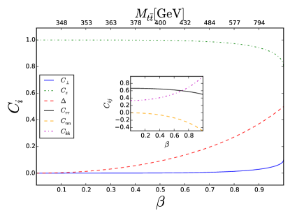
We note that the matrix is also diagonal in the helicity basis after the angular averaging since vanishes at LO due to the odd parity under inversion of the coefficient .
Moreover, a complementary entanglement signature can be obtained from , with
| (86) |
since, if all substates for fixed were separable, and so would its angular average , which satisfies . Hence, necessarily implies that some of the substates must be entangled. Another way to put it is that is an entanglement criterion for a fictitious quantum state [see discussion after Eq. (5.2)]. Similarly, one can obtain a criterion for CHSH violation that results from the angular integration of , see Eq. (2.1).
Technical details about the analytical calculation of the angular integrals are provided in Appendix D.
5.3.1 processes
We obtain for that
| (87) | ||||
while for the angular averages of the helicity spin correlations we find
| (88) | ||||
These results imply that the quantum state is completely separable as
| (89) |
We note that this only means that the angular-averaged state is separable, but not that entanglement disappears after the angular average. Indeed,
| (90) |
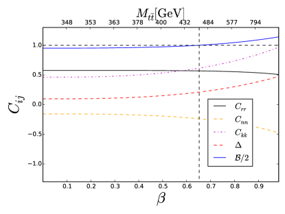
which means that entanglement is still present in the whole energy range (except exactly at threshold, ). Since in the diagonal basis , its angular average also satisfies , and thus there is CHSH violation for any non-zero , . Left Fig. 8 displays all the angular-averaged magnitudes for .
5.3.2 processes
We obtain for that
| (91) | ||||
while for the helicity spin correlations we find
| (92) | ||||
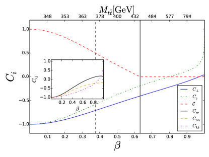
We note that for all the energies of interest (the sign crossover is produced only in the ultrarelativistic limit ). This implies that for practical purposes we can take as
| (93) |
From this expression, we compute the critical top velocity below which the state is still entangled, with the associated critical mass being .
On the other hand, since in the entangled region , can violate the CHSH inequality iff
| (94) |
This condition is satisfied below the critical value , corresponding to a critical mass .
We can also reproduce these results from the spin correlations in the helicity basis. Indeed, since
| (95) |
we have that for , and thus, in the energy range where the state is entangled, . In fact, this result can be obtained in any orthonormal basis due to the rotational invariance of the trace, , reflecting the symmetry of the spin-singlet state.
However, entanglement is again lost at high energies for : even if we use the full ,
| (96) |
we do not get any entanglement signature, in contrast to processes. Right Fig. 8 displays all the angular-averaged magnitudes for .
5.3.3 General considerations
We analyze the global results of Fig. 8 for both processes in the light of the 2D plots of Fig. 3 for . The entanglement loss in for both quark and gluon processes arises due to the statistical average over all possible top directions. However, close to threshold, gluon fusion produces a pair in a spin singlet [see Eq. (54)], invariant under rotations, and thus unaffected by the angular average, keeping the entanglement.
Nevertheless, an entanglement signature can be recovered for processes by averaging , since the helicity basis changes accordingly its orientation to produce a constructive sum of the spin correlations. The same technique does not work for the channel at high energies because there is no entanglement close to forward production , which spoils the high- entanglement when averaging over all top directions.
\stackinsetl31ptt22pt(a)
|
\stackinsetl37ptt25pt(b)
|
|---|---|
\stackinsetl31ptt22pt(c)
|
\stackinsetl39ptt25pt(d)
|
5.4 Mass integration
With the help of the angular-averaged -matrix, it is quite simple to compute expectation values in the region of phase space by integrating in the mass range specified by . Since mass integration involves luminosity functions (which we stress that do not depend on the direction), one has necessarily to consider specific hadron processes.
The angular average of the total matrix describing a realistic hadronic production process for fixed c.m. energy is
| (97) |
The actual spin density matrix is computed from its partonic counterparts as in Eq. (58):
| (98) |
where the probabilities are now
| (99) |
Finally, by Eq. (5.2), the density matrix reads in terms of these angular-averaged magnitudes as
| (100) |
with
| (101) |
Similar considerations apply to the mass integration of the angular-averaged expectation values, such as the spin correlations in the helicity basis.
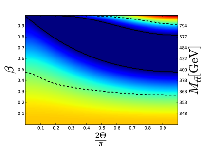
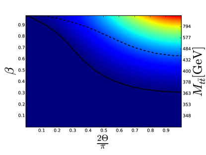
Because of their illustrative character and their high-experimental relevance, we focus on two particular hadronic processes: collisions at (very close to the actual value at the Tevatron), and collisions at (corresponding to the c.m. energy of Run 2 at the LHC). As shown in Fig. 5, at the Tevatron processes dominate while at the LHC processes do. The 2D plot of their concurrences is depicted in left column of Fig. 9. We focus on integrating the signal in the two relevant regions for entanglement: close to threshold and at high .
5.4.1 Threshold analysis
Close to threshold, the angular results of the previous subsection predict that only the channel gives rise to entangled pairs. Therefore, we restrict to the LHC example and take , which means that only events in the window are selected, so
| (102) | ||||
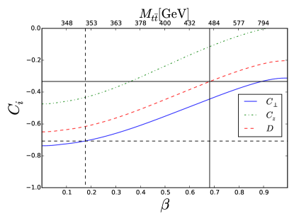
with the total integrated cross-section in the same mass window. Since it is computed in terms of the angular-averaged substates , the quantum state is also characterized by its integrated transverse and longitudinal spin correlations , represented in Fig. 9b. The necessary and sufficient condition for to be entangled is that the integrated value satisfies . Remarkably, this implies that a directly measurable entanglement witness , which satisfies only for entangled states [67], is provided by the observable of Eq. (74),
| (103) |
The concurrence is also readily computed from as . The integrated value of is represented in Fig. 9b, along with the critical value (marked by horizontal and vertical solid black lines) below which .
Regarding the CHSH violation, its presence can be also signaled by just one parameter, , as given by the condition . The critical value below which there is CHSH violation, , is marked in Fig. 9b by horizontal and vertical dashed black lines.
We compute the critical values as a function of the c.m. energy and represent them in Fig. 10. We compare these critical values with those for the angular-averaged substates , (horizontal dashed and solid lines). We observe that, for sufficiently large c.m. energies, the critical value exceeds its angular-averaged counterpart, even though contains some mixing with processes that reduces the entanglement (see lower part of right Fig. 3 and Fig. 9a). This exceeding arises from the fact that the total quantum state is a convex sum of the substates . Therefore, one needs higher energies to include a sufficient amount of separable states in order to dilute the entanglement. Nevertheless, if the integration window was entirely placed in the region of separability of , no entanglement would be observed. In contrast, for the CHSH violation, is always below its angular-averaged counterpart, at least within the range of energies considered. This is because of the critical effect introduced by the mixing with processes at threshold, see Fig. 5, which cannot be overcome by the opposite effect of mass integration due to the lower size of the CHSH-violating window. Indeed, for the considered energy of Run 2, , the weight of the channel at threshold is barely above the critical value , Fig. 5b.
5.4.2 High- analysis
For high at the Tevatron, entanglement is not present in the two-qubit quantum state but is instead signaled by the integrated value of . Indeed, Fig. 9c suggests to choose now the mass window as :
| (104) |
with . We define in a similar fashion the integrated value of the CHSH violation, .
The values of and , along with the integrated helicity spin correlations, are represented in Fig. 9d. Interestingly, even though the pairs produced close to threshold are not entangled (see lower Fig. 9c), the integration in the mass range makes in the whole mass spectrum, similarly to the increase of the critical value of for processes. However, this does not apply to the CHSH violation, which can only be observed now at high energies .
Within the angular-averaged scheme considered here, no entanglement can be detected for processes at high . We note, however, that entanglement and CHSH violation can be observed at the LHC for high if one also introduces a cut in the top direction, as suggested by Fig. 9a and implemented in Refs. [44, 45].
6 Experimental remarks
We complement here the theoretical predictions for observables of the previous section with some experimental remarks about the actual measurement scheme in high-energy colliders, and the potential statistical significance of the discovery. Nevertheless, a dedicated analysis of the expected experimental sensitivity of each prediction is beyond the scope of the present work.
6.1 Entanglement detection
The detection of entanglement is more delicate than it could be naively expected from Figs. 3, 4 since, even though entanglement is present in a wide region of phase space, one has to select carefully the phase space regions where the signal is integrated in order to obtain an entanglement signature. In fact, the recent measurement of the CMS collaboration at the LHC with the data of Run 2 [39], with no restrictions in phase space, yielded no entanglement signature, .
Our analysis reveals that there are two main regions where entanglement can be in principle detected: close to threshold and for high transverse momentum.
6.1.1 Threshold
Close to threshold, as shown in Fig. 5, the only experiment with high enough c.m. energy to give rise to entanglement is the LHC. The idea here is to measure from the cross-section of Eq. (74), applying an upper cut in the mass spectrum for the integrated signal. Although our calculation is restricted to LO, in general, the criterion still provides a sufficient condition for the entanglement of without any assumption on its specific form [see Eq. (124)].
The entanglement witness can be rewritten as the violation of a Cauchy-Schwarz inequality, a typical entanglement signature in other fields such as quantum optics, condensed matter, or analog Hawking radiation [50, 68, 69, 70]. This is proven by using the -representation of Eq. (5). If a state is separable, , and then
| (105) |
Hence, the directly measurable observable represents in the range of values a genuine non-classical feature, which can be qualitatively understood from the fact that the classical average of the scalar product of two vectors with unit length is never larger than one, . A similar entanglement criterion based on the trace of the correlation matrix was derived for Heisenberg spin chains [71].
A dedicated analysis of the entanglement discovery was performed in Refs. [41, 45], finding that high-statistical significance can be expected, potentially more than statistical deviations (), the standard candle for discovery in high-energy physics.
Figures 5, 10 show that the effect of increasing the c.m. energy saturates for large energies. Therefore, we do not expect that future hadron colliders with higher collision energies, such as possible upgrades of the LHC or the FCC, will strongly increase the entanglement in production. However, we do expect that a larger data collection will enhance the sensitivity of the measurements by reducing the statistical uncertainties. For example, the LHC is expected to collect about times more events with respect to the currently recorded data [72], a possible upgrade of the LHC to access higher energies (HE-LHC) is expected to collect about times more events [65], and the FCC is expected to collect about times more events [73]. Another possibility to increase entanglement is to enhance the contribution from the channel by further rejecting events from the channel, as recently proposed in Ref. [46].
6.1.2 High
For high , both partonic processes and give rise to the same triplet state due to orbital angular momentum dominance. Nevertheless, because the procedure used here averages over all possible top directions, only processes yield an entanglement signature in our scheme. A detailed study of the statistical significance of an entanglement detection for high at the LHC has been already provided in Ref. [45], predicting also a potential discovery.
Regarding the Tevatron, entanglement is detected from the integrated value of , which is in general a sufficient condition for the presence of entanglement [see Eq. (123)]. There are important conceptual differences between the detection of entanglement close to threshold (involving the measurement of ) and that at high (involving the measurement of ). First, close to threshold, entanglement is detected from one single magnitude, , while requires the measurement of magnitudes, which are the diagonal spin correlations in the helicity or the diagonal basis (we note that a recent work has proposed to measure also from a single parameter [46]). Second, reveals that the physical two-qubit quantum state is entangled, while signals entanglement in the fictitious quantum state , and so in the total spin-momentum quantum state .
At the Tevatron, the relatively low c.m. energy and data recorded yielded high uncertainties on spin-correlation observables [33, 34, 35]. Therefore, by considering typical uncertainties of the carried measurements, we do not expect in principle to find there an entanglement signature with high-statistical significance.
6.1.3 Lorentz invariance
Finally, we would like to discuss the possible role of the reference frame choice on the entanglement detection. While our calculations assume that the momenta for each production process are well-defined and therefore their spin-entanglement is Lorentz invariant, in realistic situations their wave function is necessarily described by wave packets with finite width, so their entanglement is no longer independent of the reference frame. However, within the current experimental scheme, the spins are by definition measured in their respective rest frames, since these are precisely the frames where the lepton directions are defined in Eq. (68).
6.2 Quantum tomography
A protocol for the quantum tomography of the pair was developed in Ref. [41], based on the fact that the experimental procedure of Section 5.1 allows to measure the integrated value of the spin correlations and spin polarizations. Thus, by implementing a cut in the invariant mass spectrum, one can extract all the parameters characterizing the total quantum state of Eq. (102). As explained, such a reconstruction requires the use of a fixed orthonormal basis in space, like the beam basis.
We extend here the proposed quantum tomography protocol to more general situations. First, we note that the protocol is not restricted to the state , but it is rather valid for any arbitrary integrated quantum state by measuring all the parameters in the beam basis. We can further simplify the process if we integrate over the azimuth around the beam axis, since then rotational invariance is recovered and thus, at LO, only parameters are needed for quantum tomography: the integrated transverse and longitudinal spin correlations . In general, by only assuming symmetry around the beam axis, the quantum tomography of the pair requires the measurement of just parameters, , with the spin polarizations along the beam axis. Nevertheless, from the recent CMS measurement [40], the values of these polarizations are still expected to be quite small. A summary of the parameters needed for the quantum tomography of the pair is presented in Table 1.
| Assumption | Coefficients | #Parameters |
|---|---|---|
| Symmetry + LO | 2 | |
| Symmetry | 4 | |
| None | 15 |
Moreover, since the quantum tomography protocol only depends on the decay properties of the pair and not on the nature of the production process, it can be extended to any production mechanism, such as positron-electron () collisions. Furthermore, even though we have focused on the case of a dileptonic decay of the pair, Eqs. (68), (5.1) are valid for any pair of detectable decay products by just replacing and by the corresponding flight directions in the parent rest frames and spin analyzing powers. We conclude by noting that the proposed quantum tomography protocol for the pair goes beyond the general approach to high-energy processes presented in Ref. [60].
6.3 CHSH violation
Since entanglement is a necessary condition for the violation of CHSH inequalities, CHSH violations are generally expected to be measured with lower statistical significance than entanglement [45]. This is clearly seen by examining Fig. 10, where we see that the upper critical value for a CHSH violation is well below that for entanglement. Remarkably, in a similar fashion to entanglement, the CHSH violation close to threshold is also inferred from the value of just one parameter, . Nevertheless, one can always measure the full CHSH violation in a more conventional way through Eq. (10). Due to the rotational invariance in the perpendicular plane to the beam, the experimental scheme is similar to the usual case of Bell inequalities with spin-singlet states, and one chooses four vectors in that plane satisfying and . Since the correlation matrix should be isotropic in this plane, this experimental scheme is equivalent to measure . We note that our choice of spin directions is fixed a priori, so no statistical bias is introduced [45].
Regarding the statistical significance of the CHSH violation close to threshold, we expect it to be much lower than that of entanglement. However, even if a significant detection is not achievable with the current Run 2 data, it could be performed with the increased c.m. energies (as seen from Fig. 10) and larger amount of data provided by future runs and/or colliders. At the Tevatron, since entanglement detection already seems quite challenging, we do not expect to achieve a statistically significant observation of a CHSH violation.
As for the case of entanglement, the scheme presented here does not allow to observe CHSH violation at the LHC at high . Nevertheless, a thorough analysis of the potential detection of CHSH violation in this regime and its statistical significance is presented in Refs. [44, 45].
So far, we have discussed the violation of the CHSH inequality of Eq. (10). However, a measurement of a genuine violation of Bell theorem implies much more than just measuring some linear combination of spin correlations above certain critical value, like in the case of entanglement. In order to fully rule out a local hidden-variable model, one needs to perform a loophole-free test that ensures that the experimental setup satisfies all the hypotheses of Bell theorem. Loophole-free violations of Bell inequalities were measured for the first time in 2015 [74, 75], and only in 2018 the so-called “free will” loophole was completely closed [76].
Consequently, a careful analysis of the measurement process in a collider is in order. Due to its illustrative character, we examine the paradigmatic case of Run 2 at the LHC. Run 2 consisted of colliding a bunch of protons every ns, yielding typically 60-80 collisions per bunch [77]. The products of these collisions are recorded by different detectors surrounding the interaction point that trace their direction and momentum/energy. This process goes on for several years (Run 1 went from 2009 to 2012, and Run 2 went from 2015 to 2018) to collect sufficient amount of statistics.
As a result, in our specific case, the experiments of Alice and Bob should be regarded as the detector recording of the pair resulting from a decay. First, one needs to ensure that the detection events are causally disconnected. This in principle could be done, since the lepton pair is typically ultrarelativistic due to the large top mass, and in addition causally-connected detection events can be rejected after reconstruction of the lepton momenta.
However, a major problem arises due to the fact that the direction of the spin measurements cannot be controlled, since we only detect the lepton directions. In fact, technically, one does not even have access to the spins, but rather infers their expectation values since they are correlated with the lepton directions. We stress that Eq. (68) is only valid after integrating out all the remaining degrees of freedom of the decay products, and cannot be used on an event by event basis. In other words: there is not a measurement setting that yields a in each detection event or that can be controlled by Alice or Bob. Therefore, the free-will loophole cannot be closed and even the specific measurement setting of the CHSH inequality is not achievable; only once the spin correlation matrix has been extracted from the fit of the angular differential cross-section of the decay products, one can aim at measuring a CHSH violation. Moreover, many of the events are not useful for the analysis, which gives rise to the so-called detection loophole.
The emergence of all these loopholes is quite natural because high-energy colliders were not specifically designed for testing Bell inequalities. As a result, in a high-energy collider, we can only detect a weak violation of the CHSH inequality, in the sense that some loopholes can never be closed. Related discussions on the validity of Bell tests in high-energy colliders can be found in Refs. [44, 45, 47].
7 Conclusions and outlook
In this work, we have provided the general framework to study the quantum state of pairs produced in QCD processes. We have discussed that, due to the nature of the measurement scheme, the most general quantum state that can be probed in a collider is fully determined by the production spin density matrix. This has to be necessarily a mixed state since a) only momentum measurements are carried out in a collider and b) one has to average over the internal degrees of freedom (like spin or color) of the initial state.
We have analyzed production for the most elementary QCD partonic reactions, extending the work of Ref. [41] to also include the analysis of CHSH violation. For processes, entanglement and CHSH violation are equivalent conditions, and are present in whole phase space. For processes, entangled pairs are produced at threshold in a spin-singlet state, and at high in a spin-triplet state, both violating the CHSH inequality. Remarkably, all these features can be essentially understood in terms of basic conservation laws of angular momentum, without invoking the specific details of QCD interactions.
We have shown that, at least at LO, any production from a real hadronic process can be written in terms of these basic building blocks through the luminosity functions, which determine the probability of a certain partonic reaction at a given c.m. energy in terms of PDF. In particular, we have focused on and collisions, which are those carried out at the LHC and the Tevatron, respectively. We have performed a detailed analysis on how the quantum state depends on the c.m. energy of the collisions, finding that at low energies the channel dominates, with the contribution increasing with the c.m. energy for both types of collisions. For the LHC, the channel already dominates at the energies of its first run. For the Tevatron, however, due to its relatively low-energy operating point, processes dominate. Thus, both colliders represent a perfect example of each elementary QCD process.
Thinking about potential experimental realizations, we have proposed a number of realistic observables for the characterization of the quantum state that provide signatures of entanglement and CHSH violation. Interestingly, at the LHC these signatures are obtained by the measurement of a single magnitude: for entanglement, the trace of the correlation matrix is a good entanglement witness, as already predicted in Ref. [41], while CHSH violation can be signaled by measuring the spin correlations in the transverse plane to the beam.
Finally, we analyze in detail the experimental implementation of these ideas. We explicitly show that an entanglement measurement at the LHC represents the violation of a Cauchy-Schwarz inequality. Regarding the Tevatron, we find that a statistically significant observation of entanglement seems quite challenging due to the relatively large expected uncertainties.
We also extend the quantum tomography protocol developed in Ref. [41] to more general quantum states, arguing that it can be applied in general to any quantum state. In particular, if one averages over the beam axis, rotational symmetry is recovered and the quantum tomography can be implemented from the measurement of just parameters, related to the transverse and longitudinal spin correlations, and to the longitudinal spin polarizations. Furthermore, since the protocol does not depend on the specific production process, it can be extended to any production mechanism, like electroweak production from collisions.
Regarding the CHSH violation, since it is a stronger requirement than entanglement, its statistical significance is expected to be lower. Moreover, we argue that, due to the nature of the detection process, only weak violations of Bell inequalities can be measured in a high-energy collider, since some loopholes, like those related to the free-will or to the detection efficiency, cannot be closed. This is not surprising: after all, high-energy colliders were not designed to test Bell inequalities.
From a quantum information perspective, top quarks allow to export fundamental concepts in quantum information, such as entanglement, CHSH violation or quantum tomography, to the high-energy field. This opens the prospect of using high-energy colliders to study quantum information problems at the highest-energy scale available. The genuine relativistic behavior, the exotic character of the interactions and symmetries involved, and the fundamental nature of this environment make it especially attractive for such purpose. Indeed, the detection of entanglement or CHSH violation in pairs would represent their highest-energy detections ever, many orders of magnitude above standard laboratory setups. Another interesting experiment is the implementation of the quantum tomography of the pair, which could be used for instance to measure quantum discord [78, 79].
A very interesting perspective is provided by future colliders, where pairs are expected to be produced from collisions, such as the FCC- [80]. In particular, in future linear colliders such as the International Linear Collider (ILC) [81] and the the Compact Linear Collider (CLIC) [82, 83], spin degrees of the initial state can be controlled to a large extent, in contrast to the QCD production discussed in this work. These colliders are then revealed as quite promising scenarios to study quantum information problems, where the techniques of this work can be straightforwardly adapted. Alternative candidates to top quarks for the study of quantum information problems are gauge bosons arising from Higgs decays and leptons [47, 84, 43].
From the high-energy perspective, the introduction of quantum information concepts can provide new relevant observables in the field. For example, entanglement measurements can help to understand the underlying mechanism of a certain production process. A very intriguing extension of this work is to explore New Physics beyond the Standard Model by measuring the quantum state of the pair, comparing the experimental results with the predictions of the different theories available. Indeed, some recent works already address the possibility of using entanglement to trace signatures of New Physics [42, 43].
We conclude by stressing that the work has been fully developed within a genuine quantum information framework, since once the production spin density matrix and the luminosity functions are computed by the theory of high-energy physics, all the calculations are reduced to study convex combinations of two-qubit quantum states using standard tools of quantum information theory. Our work then provides a simple and general approach for non-particle physicists to the quantum information aspects of high-energy colliders, a fascinating arena to study the foundations of quantum mechanics.
Acknowledgements
We thank E. Madge, M. Vos, F. Sols, G. Sierra and J. J. García-Ripoll for valuable comments. JRMdN acknowledges funding from European Union’s Horizon 2020 research and innovation programme under the Marie Skłodowska-Curie grant agreement No 847635, and also from Grant FIS2017-84368-P from Spain’s MINECO.
Appendix A -representation and coherent states for qudits
We review here the main properties of the -representation for qudits introduced in Ref. [85]. We describe a Hilbert space of dimension as an irreducible representation of SU(2) with angular momentum such that . The qudit basis is relabeled as , with the eigenvalues of the -component of the angular momentum, . Angular momentum coherent states are defined as those simultaneously eigenstates of and , i.e., and , where we work in the usual orthonormal basis in spherical coordinates :
| (106) | ||||
One can easily compute from the ladder operators as , finding
| (107) |
As the more usual coherent states, these states form an overcomplete basis of the Hilbert space,
| (108) |
The -representation for a quantum state is defined from these coherent states as
| (109) |
This definition does not completely fix . In order to check it, we consider its expansion in spherical harmonics
| (110) | ||||
where are the associated Legendre polynomials. Normalization of implies . Since spherical harmonics form an orthonormal basis, when inserting Eq. (A) in Eq. (109) we realize that only the coefficients with are involved, while those for remain undetermined. Thus, the most general expression for is
| (111) |
with the projector onto and an arbitrary angular function. Since is a real function, the number of real parameters determining the coefficients is precisely , the number of parameters fixing an arbitrary density matrix in a Hilbert space of dimension . Therefore, any density matrix can be described in terms of a certain function , where those admitting a non-negative -function represent classical states described by a conventional probability distribution.
We now focus on the case of qubits, where and the coherent states are the usual spin states
| (112) |
where are the spin states along the -axis, . Since , only spherical harmonics up to in the expansion of are involved in the expression of . This can be straightforwardly checked by noticing in Eq. (2) that
| (113) |
Moreover, if we choose the basis for the spherical harmonics , we simply find that the coefficients of Eq. (1) are
| (114) |
and thus
| (115) |
For one qubit, a non-negative can always be found since is in fact an incoherent mixture of the two spin states along the direction of the Bloch vector .
The two-qubit case is straightforwardly adapted from the one qubit case. In particular, the most general expression for , defined through Eq. (5), is now
| (116) |
Entangled states are thus states for which no can be found such that is non-negative.
Appendix B Specific entanglement criteria for pairs
We derive here some adapted results for quantum states from the general entanglement criteria discussed in Section 2.1. For that purpose, we write the full matrix form of the general expression for a density matrix in a Hilbert space, Eq. (4):
|
|
(117) |
where we are following the usual convention for the Pauli matrices . For the analysis of the Peres-Horodecki criterion, we compute the partial transpose of with respect to the second subsystem, , which amounts to transpose its four blocks, namely:
|
|
(118) |
The Peres-Horodecki criterion states that is non-negative iff is separable. A simpler version of this statement is obtained by considering vectors with only first and fourth component, which gives a reduced quadratic form
| (119) |
The non-negative character of implies . Thus, is a sufficient condition of entanglement since it implies that is not positive semi-definite. In turn, can be rewritten as , with
| (120) |
Furthermore,
| (121) |
so provides an even simpler entanglement criterion. Specifically, since , iff
| (122) |
Thus, the entanglement signatures used in the main text
| (123) |
as well as
| (124) |
are sufficient conditions for entanglement in general, valid for arbitrary quantum states in bipartite Hilbert spaces.
We now address the specific case of production through LO QCD, characterized by unpolarized quantum states (the so-called -states [86]), , and a symmetric correlation matrix, . The latter condition implies that the correlation matrix can be diagonalized after the appropriated rotation, , which reduces Eq. (117) to
|
|
(125) |
It is easy to see that
| (126) |
by demanding to be a physical state described by a non-negative density matrix. This complements the Peres-Horodecki criterion, which says that the state is entangled iff
| (127) |
By combining both conditions, we find that Peres-Horodecki is equivalent to
| (128) | ||||
where the first line is just the condition of Eq. (123).
For a -state, the concurrence can be also analytically computed from its definition (8), since in that case . Hence, , and are the eigenvalues of , , . Moreover, as has unit trace,
| (129) |
and the concurrence is simply , with . By noting the analogy with Eq. (127), we can write the concurrence directly in terms of the Peres-Horodecki criterion:
| (130) |
For the study of the angular-averaged quantum states , we consider the particular case in which there is invariance under rotations around a certain direction, chosen along and labeled as the -axis. In that case, the spin polarizations must be longitudinal, , and the correlation matrix is diagonal, , with eigenvalues and . The Peres-Horodecki criterion is then equivalent to
| (131) |
If the state is unpolarized,
| (132) |
is a necessary and sufficient condition for entanglement, while for , is just a sufficient condition.
Appendix C Parton distribution functions
We further explain here the concept of PDF and detail how the luminosity functions of Eq. (56) are computed. The PDF determines the probability of originating a parton from the corresponding hadron with an energy fraction . For instance, in the case of collisions, a pair is originated from the interaction between a parton from one of the protons and the corresponding antiparton from the other proton. The probability of producing a state with partonic c.m. energy is . In the case of , can be either some light quark, , or its corresponding antiparticle . In the case of , is a gluon. Since the partonic c.m. frame is that of the pair, the c.m. energy is the same, , and thus we can compute the luminosity function as
| (133) |
where the sum over the index runs over all the possible partons giving rise to the state . Changing to dimensionless variables , gives
| (134) |
For the case of collisions, we simply replace one of the proton PDF above by the antiproton PDF , which is that of the proton but interchanging partons with antipartons, .
Appendix D Angular averaging
We outline here the main technical details about the computation of the angular integrals presented in Section 5.3.
D.0.1 processes
For computing the angular averages involved in the channel, the polar integrals in can be computed either as polynomials in or in terms of
| (135) |
with the usual Euler gamma function.
The integral giving rise to the CHSH violation is much more delicate. We sketch here the main steps for its computation. First, we change variable as , so
| (136) |
This last integral can be recurrently rewritten after integrating by parts as
| (137) | |||
with
| (138) |
This integral can be in turn expressed in terms of elliptic integrals:
| (139) | ||||
where
| (140) | ||||
The last step is changing to angular variables as
| (141) | ||||
which yields
| (142) | |||
In the above equation, is the modulus of the elliptic integral, and , with
| (143) |
The integrals can be analitically obtained in terms of elliptic functions. For instance,
| (144) |
is just the usual incomplete elliptic integral of the first kind, which through the relation defines the Jacobi elliptic functions
| (145) |
These functions allow to rewrite
| (146) |
This integral can be computed analytically through recurrence relations. Nevertheless, the values of for , needed for the computation of , are too cumbersome to write them here; we refer the interested reader to Ref. [88] for its complete expressions. For any practical purpose, we find that direct numerical integration of Eq. (D.0.1) is faster and simpler.
D.0.2 production
For processes, it can be seen that all the involved integrals can be put in terms of , with
| (147) |
This integral satisfies recursion relations
| (148) | ||||
that eventually yield
| (149) | ||||
References
- [1] Albert Einstein, Boris Podolsky, and Nathan Rosen. “Can quantum mechanical description of physical reality be considered complete?”. Phys. Rev. 47, 777–780 (1935).
- [2] E. Schrodinger. “Discussion of probability relations between separated systems”. Pro. Cambridge Phi. Soc. 31, 555 (1935).
- [3] J. S. Bell. “On the Einstein-Podolsky-Rosen paradox”. Physics Physique Fizika 1, 195–200 (1964).
- [4] Charles H. Bennett, Gilles Brassard, Claude Crépeau, Richard Jozsa, Asher Peres, and William K. Wootters. “Teleporting an unknown quantum state via dual classical and Einstein-Podolsky-Rosen channels”. Phys. Rev. Lett. 70, 1895–1899 (1993).
- [5] Dik Bouwmeester, Jian-Wei Pan, Klaus Mattle, Manfred Eibl, Harald Weinfurter, and Anton Zeilinger. “Experimental quantum teleportation”. Nature 390, 575–579 (1997).
- [6] Daniel Gottesman and Isaac L. Chuang. “Demonstrating the viability of universal quantum computation using teleportation and single-qubit operations”. Nature 402, 390–393 (1999).
- [7] Charles H Bennett and David P DiVincenzo. “Quantum information and computation”. Nature 404, 247 (2000).
- [8] Robert Raussendorf and Hans J. Briegel. “A one-way quantum computer”. Phys. Rev. Lett. 86, 5188–5191 (2001).
- [9] Nicolas Gisin, Grégoire Ribordy, Wolfgang Tittel, and Hugo Zbinden. “Quantum cryptography”. Rev. Mod. Phys. 74, 145–195 (2002).
- [10] Vittorio Giovannetti, Seth Lloyd, and Lorenzo Maccone. “Quantum-enhanced measurements: Beating the standard quantum limit”. Science 306, 1330–1336 (2004).
- [11] Robert M. Gingrich and Christoph Adami. “Quantum entanglement of moving bodies”. Phys. Rev. Lett. 89, 270402 (2002).
- [12] Asher Peres and Daniel R. Terno. “Quantum information and relativity theory”. Rev. Mod. Phys. 76, 93–123 (2004).
- [13] Nicolai Friis, Reinhold A. Bertlmann, Marcus Huber, and Beatrix C. Hiesmayr. “Relativistic entanglement of two massive particles”. Phys. Rev. A 81, 042114 (2010).
- [14] N. Friis, A. R. Lee, K. Truong, C. Sabín, E. Solano, G. Johansson, and I. Fuentes. “Relativistic quantum teleportation with superconducting circuits”. Phys. Rev. Lett. 110, 113602 (2013).
- [15] Flaminia Giacomini, Esteban Castro-Ruiz, and Časlav Brukner. “Relativistic quantum reference frames: The operational meaning of spin”. Phys. Rev. Lett. 123, 090404 (2019).
- [16] Podist Kurashvili and Levan Chotorlishvili. “Quantum discord and entropic measures of two relativistic fermions” (2022). arXiv:2207.12963.
- [17] Albert Bramon and Gianni Garbarino. “Novel Bell’s inequalities for entangled pairs”. Phys. Rev. Lett. 88, 040403 (2002).
- [18] Yu Shi. “Entanglement in relativistic quantum field theory”. Phys. Rev. D 70, 105001 (2004).
- [19] Boris Kayser, Joachim Kopp, R. G. Hamish Robertson, and Petr Vogel. “Theory of neutrino oscillations with entanglement”. Phys. Rev. D 82, 093003 (2010).
- [20] Alba Cervera-Lierta, José I. Latorre, Juan Rojo, and Luca Rottoli. “Maximal entanglement in High Energy Physics”. SciPost Phys. 3, 036 (2017).
- [21] Zhoudunming Tu, Dmitri E. Kharzeev, and Thomas Ullrich. “Einstein-Podolsky-Rosen paradox and quantum entanglement at subnucleonic scales”. Phys. Rev. Lett. 124, 062001 (2020).
- [22] X. Feal, C. Pajares, and R. A. Vazquez. “Thermal and hard scales in transverse momentum distributions, fluctuations, and entanglement”. Phys. Rev. C 104, 044904 (2021).
- [23] S. Abachi et al. “Observation of the top quark”. Phys. Rev. Lett. 74, 2632–2637 (1995). arXiv:hep-ex/9503003.
- [24] F. Abe et al. “Observation of top quark production in collisions”. Phys. Rev. Lett. 74, 2626–2631 (1995). arXiv:hep-ex/9503002.
- [25] G. L. Kane, G. A. Ladinsky, and C. P. Yuan. “Using the top quark for testing standard-model polarization and predictions”. Phys. Rev. D 45, 124–141 (1992).
- [26] Werner Bernreuther and Arnd Brandenburg. “Tracing violation in the production of top quark pairs by multiple tev proton-proton collisions”. Phys. Rev. D 49, 4481–4492 (1994).
- [27] Stephen J. Parke and Yael Shadmi. “Spin correlations in top quark pair production at colliders”. Phys. Lett. B 387, 199–206 (1996). arXiv:hep-ph/9606419.
- [28] W. Bernreuther, M. Flesch, and P. Haberl. “Signatures of Higgs bosons in the top quark decay channel at hadron colliders”. Phys. Rev. D 58, 114031 (1998).
- [29] W. Bernreuther, A. Brandenburg, Z.G. Si, and P. Uwer. “Top quark pair production and decay at hadron colliders”. Nuclear Physics B 690, 81 – 137 (2004).
- [30] Peter Uwer. “Maximizing the spin correlation of top quark pairs produced at the large hadron collider”. Physics Letters B 609, 271 – 276 (2005).
- [31] Matthew Baumgart and Brock Tweedie. “A new twist on top quark spin correlations”. Journal of High Energy Physics 2013, 117 (2013).
- [32] Werner Bernreuther, Dennis Heisler, and Zong-Guo Si. “A set of top quark spin correlation and polarization observables for the LHC: Standard Model predictions and new physics contributions”. Journal of High Energy Physics 2015, 1–36 (2015).
- [33] T. Aaltonen et al. “Measurement of Spin Correlation in Collisions Using the CDF II Detector at the Tevatron”. Phys. Rev. D83, 031104 (2011). arXiv:1012.3093.
- [34] Victor Mukhamedovich Abazov et al. “Measurement of spin correlation in production using a matrix element approach”. Phys. Rev. Lett. 107, 032001 (2011). arXiv:1104.5194.
- [35] Victor Mukhamedovich Abazov et al. “Measurement of Spin Correlation between Top and Antitop Quarks Produced in Collisions at 1.96 TeV”. Phys. Lett. B757, 199–206 (2016). arXiv:1512.08818.
- [36] Georges Aad et al. “Observation of spin correlation in events from pp collisions at sqrt(s) = 7 TeV using the ATLAS detector”. Phys. Rev. Lett. 108, 212001 (2012). arXiv:1203.4081.
- [37] Serguei Chatrchyan et al. “Measurements of spin correlations and top-quark polarization using dilepton final states in collisions at = 7 TeV”. Phys. Rev. Lett. 112, 182001 (2014). arXiv:1311.3924.
- [38] Georges Aad et al. “Measurement of Spin Correlation in Top-Antitop Quark Events and Search for Top Squark Pair Production in Collisions at TeV Using the ATLAS Detector”. Phys. Rev. Lett. 114, 142001 (2015). arXiv:1412.4742.
- [39] Albert M Sirunyan et al. “Measurement of the top quark polarization and spin correlations using dilepton final states in proton-proton collisions at 13 TeV”. Phys. Rev. D100, 072002 (2019). arXiv:1907.03729.
- [40] Morad Aaboud et al. “Measurements of top-quark pair spin correlations in the channel at TeV using collisions in the ATLAS detector”. Eur. Phys. J. C 80, 754 (2020). arXiv:1903.07570.
- [41] Yoav Afik and Juan Ramón Muñoz de Nova. “Entanglement and quantum tomography with top quarks at the LHC”. The European Physical Journal Plus 136, 1–23 (2021). arXiv:2003.02280.
- [42] Rafael Aoude, Eric Madge, Fabio Maltoni, and Luca Mantani. “Quantum SMEFT tomography: Top quark pair production at the LHC”. Phys. Rev. D 106, 055007 (2022). arXiv:2203.05619.
- [43] Marco Fabbrichesi, Roberto Floreanini, and Emidio Gabrielli. “Constraining new physics in entangled two-qubit systems: top-quark, tau-lepton and photon pairs” (2022). arXiv:2208.11723.
- [44] M. Fabbrichesi, R. Floreanini, and G. Panizzo. “Testing Bell inequalities at the LHC with top-quark pairs”. Phys. Rev. Lett. 127, 161801 (2021). arXiv:2102.11883.
- [45] Claudio Severi, Cristian Degli Esposti Boschi, Fabio Maltoni, and Maximiliano Sioli. “Quantum tops at the LHC: from entanglement to Bell inequalities”. The European Physical Journal C 82, 285 (2022). arXiv:2110.10112.
- [46] J. A. Aguilar-Saavedra and J. A. Casas. “Improved tests of entanglement and Bell inequalities with LHC tops”. The European Physical Journal C 82, 666 (2022). arXiv:2205.00542.
- [47] Alan J. Barr. “Testing Bell inequalities in Higgs boson decays”. Phys. Lett. B 825, 136866 (2022). arXiv:2106.01377.
- [48] Andrew J. Larkoski. “General analysis for observing quantum interference at colliders”. Phys. Rev. D 105, 096012 (2022).
- [49] Werner Bernreuther and Zong-Guo Si. “Distributions and correlations for top quark pair production and decay at the Tevatron and LHC”. Nucl. Phys. B 837, 90–121 (2010). arXiv:1003.3926.
- [50] D.F. Walls and G.J. Milburn. “Quantum optics”. Springer-Verlag. Berlin, Heidelberg, New York (2008).
- [51] Asher Peres. “Separability criterion for density matrices”. Phys. Rev. Lett. 77, 1413–1415 (1996).
- [52] Pawel Horodecki. “Separability criterion and inseparable mixed states with positive partial transposition”. Physics Letters A 232, 333 – 339 (1997).
- [53] William K. Wootters. “Entanglement of formation of an arbitrary state of two qubits”. Phys. Rev. Lett. 80, 2245–2248 (1998).
- [54] Daniel F. V. James, Paul G. Kwiat, William J. Munro, and Andrew G. White. “Measurement of qubits”. Phys. Rev. A 64, 052312 (2001).
- [55] John F. Clauser, Michael A. Horne, Abner Shimony, and Richard A. Holt. “Proposed experiment to test local hidden-variable theories”. Phys. Rev. Lett. 23, 880–884 (1969).
- [56] R. Horodecki, P. Horodecki, and M. Horodecki. “Violating Bell inequality by mixed spin-12 states: necessary and sufficient condition”. Physics Letters A 200, 340–344 (1995).
- [57] B. S. Cirel’son. “Quantum generalizations of Bell’s inequality”. Letters in Mathematical Physics 4, 93–100 (1980).
- [58] J.R. Taylor. “Scattering theory: The quantum theory of nonrelativistic collisions”. Dover. New York (2006).
- [59] Dmitri E. Kharzeev and Eugene M. Levin. “Deep inelastic scattering as a probe of entanglement”. Phys. Rev. D 95, 114008 (2017).
- [60] John C. Martens, John P. Ralston, and J. D. Tapia Takaki. “Quantum tomography for collider physics: Illustrations with lepton pair production”. Eur. Phys. J. C 78, 5 (2018). arXiv:1707.01638.
- [61] Gregory Mahlon and Stephen Parke. “Angular correlations in top quark pair production and decay at hadron colliders”. Phys. Rev. D 53, 4886–4896 (1996).
- [62] R. P. Feynman. “The behavior of hadron collisions at extreme energies”. Conf. Proc. C 690905, 237–258 (1969).
- [63] J.D. Bjorken and Emmanuel A. Paschos. “Inelastic Electron Proton and gamma Proton Scattering, and the Structure of the Nucleon”. Phys. Rev. 185, 1975–1982 (1969).
- [64] Stephane Fartoukh et al. “LHC Configuration and Operational Scenario for Run 3”. Technical report. CERNGeneva (2021). url: cds.cern.ch/record/2790409.
- [65] A. Abada et al. “HE-LHC: The High-Energy Large Hadron Collider: Future Circular Collider Conceptual Design Report Volume 4”. Eur. Phys. J. ST 228, 1109–1382 (2019).
- [66] Michael Benedikt, Alain Blondel, Patrick Janot, Michelangelo Mangano, and Frank Zimmermann. “Future Circular Colliders succeeding the LHC”. Nature Phys. 16, 402–407 (2020).
- [67] Barbara M. Terhal. “Bell inequalities and the separability criterion”. Physics Letters A 271, 319–326 (2000).
- [68] Sabine Wölk, Marcus Huber, and Otfried Gühne. “Unified approach to entanglement criteria using the Cauchy-Schwarz and Hölder inequalities”. Phys. Rev. A 90, 022315 (2014).
- [69] J. R. M. de Nova, F. Sols, and I. Zapata. “Violation of Cauchy-Schwarz inequalities by spontaneous Hawking radiation in resonant boson structures”. Phys. Rev. A 89, 043808 (2014).
- [70] J. R. M. de Nova, F. Sols, and I. Zapata. “Entanglement and violation of classical inequalities in the Hawking radiation of flowing atom condensates”. New J. Phys. 17, 105003 (2015). arXiv:1509.02224.
- [71] John Schliemann. “Entanglement in su(2)-invariant quantum spin systems”. Phys. Rev. A 68, 012309 (2003).
- [72] I. Zurbano Fernandez et al. “High-Luminosity Large Hadron Collider (HL-LHC): Technical design report”. Technical report. CERNGeneva (2020).
- [73] A. Abada et al. “FCC-hh: The Hadron Collider: Future Circular Collider Conceptual Design Report Volume 3”. Eur. Phys. J. ST 228, 755–1107 (2019).
- [74] B. Hensen et al. “Loophole-free Bell inequality violation using electron spins separated by 1.3 kilometres”. Nature 526, 682–686 (2015). arXiv:1508.05949.
- [75] Marissa Giustina, Marijn A. M. Versteegh, Sören Wengerowsky, Johannes Handsteiner, Armin Hochrainer, Kevin Phelan, Fabian Steinlechner, Johannes Kofler, Jan-Åke Larsson, Carlos Abellán, Waldimar Amaya, Valerio Pruneri, Morgan W. Mitchell, Jörn Beyer, Thomas Gerrits, Adriana E. Lita, Lynden K. Shalm, Sae Woo Nam, Thomas Scheidl, Rupert Ursin, Bernhard Wittmann, and Anton Zeilinger. “Significant-loophole-free test of Bell’s Theorem with entangled photons”. Phys. Rev. Lett. 115, 250401 (2015).
- [76] The BIG Bell Test Collaboration. “Challenging local realism with human choices”. Nature 557, 212–216 (2018).
- [77] Georges Aad et al. “Operation of the ATLAS trigger system in Run 2”. JINST 15, P10004 (2020). arXiv:2007.12539.
- [78] Harold Ollivier and Wojciech H. Zurek. “Quantum discord: A measure of the quantumness of correlations”. Phys. Rev. Lett. 88, 017901 (2001).
- [79] Yoav Afik and Juan Ramón Muñoz de Nova. “Quantum discord and steering in top quarks at the LHC” (2022). arXiv:2209.03969.
- [80] Alain Blondel et al. “Polarization and Centre-of-mass Energy Calibration at FCC-ee” (2019). arXiv:1909.12245.
- [81] T. Barklow, J. Brau, K. Fujii, J. Gao, J. List, N. Walker, and K. Yokoya. “ILC Operating Scenarios” (2015). arXiv:1506.07830.
- [82] M J Boland et al. “Updated baseline for a staged Compact Linear Collider” (2016). arXiv:1608.07537.
- [83] T. K. Charles et al. “The Compact Linear Collider (CLIC) - 2018 Summary Report” (2018). arXiv:1812.06018.
- [84] Alan J. Barr, Pawel Caban, and Jakub Rembieliński. “Bell-type inequalities for systems of relativistic vector bosons” (2022). arXiv:2204.11063.
- [85] Olivier Giraud, Petr Braun, and Daniel Braun. “Classicality of spin states”. Phys. Rev. A 78, 042112 (2008).
- [86] Ryszard Horodecki and Michal/ Horodecki. “Information-theoretic aspects of inseparability of mixed states”. Phys. Rev. A 54, 1838–1843 (1996).
- [87] Richard D. Ball et al. “Parton distributions for the LHC Run II”. JHEP 04, 040 (2015). arXiv:1410.8849.
- [88] Paul F. Byrd and Morris D. Friedman. “Handbook of Elliptic Integrals for Engineers and Scientists”. Springer-Verlag. Berlin, Heidelberg, New York (1971).
