Autofocusing+: Noise-Resilient Motion Correction in Magnetic Resonance Imaging

Abstract

Image corruption by motion artifacts is an ingrained problem in Magnetic Resonance Imaging (MRI). In this work, we propose a neural network-based regularization term to enhance Autofocusing, a classic optimization-based method to remove motion artifacts. The method takes the best of both worlds: the optimization-based routine iteratively executes the blind demotion and deep learning-based prior penalizes for unrealistic restorations and speeds up the convergence. We validate the method on three models of motion trajectories, using synthetic and real noisy data. The method proves resilient to noise and anatomic structure variation, outperforming the state-of-the-art demotion methods.

1 Introduction

Magnetic Resonance Imaging (MRI) non-invasively measures precise anatomical and functional patterns within the human body. During the scan, it is nearly impossible for the patients to remain still in the scanner, with the movement of several millimeters or more being typical even for a healthy adult [7]. Despite delivering superb detail and accelerating the acquisition, powerful MRI machines are invariably prone to motion artifacts. This stems from the voxels of the modern sensors, such as those in the high-resolution 7-Tesla scanners, so small that even a miniature patient movement results in severe voxel displacements [10].

Generally, motion artifacts degrade the scan’s quality, manifesting themselves as ghosting or blurring in the image [33]. The nature of these artifacts is convoluted, with many possible causing factors, ranging from the motion of an inner organ to that of the scanned body part, to the specifics of the k-space trajectory in the signal acquisition protocol, to the patient’s trembling, etc. The periodic movements, such as cardiac motion and arterial pulsation, introduce distinctive well-defined patterns, whereas an arbitrary motion of the patient leads to a uniform image blur [35, 8].

Motion artifacts lessen the overall diagnostic value of MRI data and may lead to misinterpretation when confused with pathology. The effect of motion alone, e.g., is estimated to introduce a 4% error into the measurement of the gray matter in the brain [23]. That is especially crucial on the low signal-to-noise ratio (SNR) scans in the presence of noise or when the pathology is smaller than the voxel size of the scanner. Compensating for the motion artifacts is referred to as demotion and is one of the most important tasks in the medical vision.

Related Work.

The demotion methods can be broadly classified into prospective (during the scan, e.g., [19]) and retrospective (after the scan, e.g., [20]).

In the latter category, ‘Autofocusing’ [2] optimization algorithm became classic, allowing the motion parameters to be found iteratively with respect to a chosen quality metric and assuming the image corruption model is known. Any such model, however, is hardly universal, given the omni-directional and non-uniform movements make the selection of a proper metric problematic [17]. Perception-based metrics could alleviate the challenge [30, 5]; however, MRI-specific standards for visual evaluation of motion artifacts do not exist [29].

Another powerful optimization-based Autofocusing method to remove motion artifacts is GradMC [15], the latest version of which compensates for nonrigid physiological motions by distilling local rigid motion of separate patches of the image. Instrumental in some cases, the method fails to handle sufficiently large movements and is computationally complex. In the presence of certain noise levels or when an object’s structure varies abruptly GradMC underperforms and can introduce new artefacts.

With the advent of deep learning, the optimization methods were somewhat substituted by the convolutional neural networks (CNNs) [9, 1, 13], improving convergence of the non-convex motion parameter optimization procedure and/or increasing the reconstruction quality. A plethora of CNN-based deblurring methods, such as popular DnCNN [37], have then been implemented [29, 30], without taking the physical nature of the MRI artifacts into account. Same applies to a generative adversarial network (GAN) approach MedGAN [13], entailing extra adversarial loss functions and the associated long training routine.

In the majority of works on MRI demotion, the corrupted data are either private [13, 30] or generated by a model [1, 29, 5]. Herein, we also resort to the latter and employ a physics-based model to introduce the artifacts.

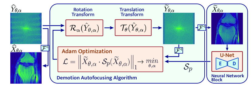
We propose to enhance the widely used Autofocusing algorithm by a CNN-extracted prior knowledge about k-space specific motion corruption model, adding to the popular algorithm the new attributes of stability to anatomic structure variation and resilience to noise. Fig. 1 summarizes the proposed method.

Figure 1: Autofocusing+: proposed demotion method. The classic Autofocusing output $\widetilde{Y}_{\theta,\alpha}$ (left) is iteratively regularized with U-Net prior $\mathcal{S}_{p}(\widetilde{Y}_{\theta,\alpha})$(right). The L1-minimization of the regularized output updates the motion parameters $\theta$ and $\alpha$.

2 Methods

2.0.1 Motion Artifact Model.

Figure 2: MR image corrupted with different motion artifact trajectories in k-space (insets show the corresponding spectra). Second raw: corresponding motion vectors. The movement trajectories considered: single-sine, multi-sine (or harmonic), and random (random contribution of multiple waves to the overall trajectory).

We restrict the modeling to the problem of rigid body movements. The corrupted image $\hat{X}_{\theta,\alpha}$ can be obtained via sequential affine transforms of the clean image $X$: rotation $\mathcal{R}_{\alpha}(\cdot)$ and translation $\mathcal{T}_{\theta}(\cdot)$, characterized in the k-space domain by the trajectory parameters $\alpha$ and $\theta$, respectively [2]). Denoting $Y=\mathcal{F}(X)$ as the Fourier transform,

$$\hat{X}_{\theta,\alpha}=\mathcal{F}^{-1}(\mathcal{R}_{\alpha}(\mathcal{T}_{\theta}(Y)))\,.$$ (1)

In practice, the k-space rotation is performed by multiplying each column of the coordinate grid $G$ by a rotation matrix:

$$G_{\alpha}=\left[\begin{array}[]{cc}\cos\alpha&\sin\alpha\\ -\sin\alpha&\cos\alpha\end{array}\right]\cdot G\,,$$ (2)

which destroys the uniformity of the equispaced periodic frequencies and requires methods, such as Non-Uniform Fourier Transform (NUFFT) [6], to place the frequency components on a new uniform grid correctly:

$$\mathcal{R}_{\alpha}(Y)=\text{NUFFT}(Y,G_{\alpha})\,.$$ (3)

Likewise, the translation operation can be formalized as:

$$\mathcal{T}_{\theta}(Y)=|Y|\,\text{exp}(-j2\pi\angle Y+\theta)\,,$$ (4)

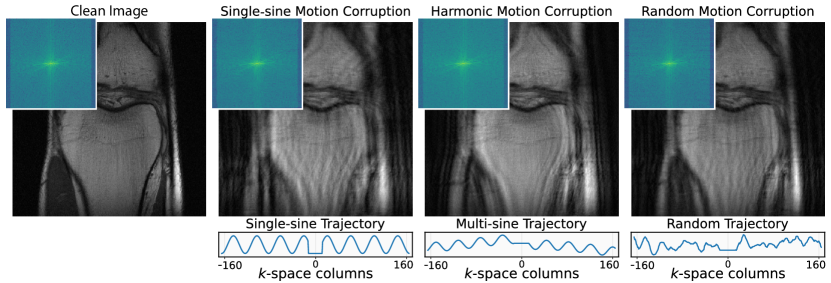
where $\theta$ is the shift parameter, $\angle Y$ and $|Y|$ are the angle and the magnitude of the complex values of $Y$. The motion artifacts, generated by Eqns. (3) and (4), have to be reversible ($\mathcal{T}^{-1}_{\theta}(\mathcal{T}_{\theta}(X))=X$, $\mathcal{R}^{-1}_{\alpha}(\mathcal{R}_{\alpha}(X))=X$) and commutative ($\mathcal{T}_{\theta}(\mathcal{R}_{\alpha}(X))=\mathcal{R}_{\alpha}(\mathcal{T}_{\theta}(X))$). The motion vectors, set by various configurations of harmonic trajectories and parametrized by $\alpha$ and $\theta$, along with the modified k-space and the resulting artifacts are shown in Fig. 2.

2.0.2 Autofocusing+ Algorithm.

The optimization task of finding motion trajectories can be formulated as a blind demotion, because the amplitude and the motion trajectory are unknown:

$$\operatorname*{argmin}_{\theta,\alpha}\left\|\hat{X}_{\theta,\alpha}\right\|_{1}\,.$$ (5)

For the optimization routine (ref. Algorithm 1), previously conjugate gradient and LBFGS were used, but because of the computational complexity of our method, we apply basic Adam gradient descent [11] to iteratively update the motion vectors w.r.t. the image quality metric. Inspired by previous studies [16][34], L1-norm was used as the image quality measure $\mathcal{L}_{AF}$. The L1-norm choice is rational because the motion artifacts blur sharp edges in the image and, therefore, decrease the image sparsity by ‘redistributing’ intensity values between the neighboring pixels. Below, the Adam-based autofocusing algorithm is referred to as ‘baseline Autofocusing’.

Algorithm 1 Autofocusing+ Optimization

0:  $\hat{Y}_{\theta,\alpha}\in\mathbb{C}^{n\times n}$ // k-space corrupted by motion with parameters $\theta,\alpha$

0:  $\tilde{Y}_{\theta,\alpha}\in\mathbb{C}^{n\times n}$ // Refined k-space

  for train epoch do

     for optimization step do

        Compute image quality metric $\mathcal{L}_{AF}=\left\|\hat{X}_{\theta,\alpha}\cdot\mathcal{S}_{p}(\hat{X}_{\theta,\alpha})\right\|_{1}$

        Calculate gradients for Autofocusing parameters $\theta$, $\alpha$

        Update Autofocusing parameters $\theta,\alpha$ with Adam Gradient Descent

     end for

     Compute loss between target and refined image $\mathcal{L}_{NN}(\hat{X}_{\theta,\alpha},X)$

     Calculate gradients for Neural Network parameters $p$

     Update Neural Network parameters $p$ with Adam Gradient Descent

  end for

2.0.3 U-Net as an Additional Prior.

Our idea is to use a CNN alongside the image quality metric in the optimization procedure to improve the image restoration quality via an additional image prior [12, 28]. Naturally, a simple U-Net [24] architecture was considered for such a regularization task.

Importantly, in the proposed pipeline (See Fig.1), the CNN is the part of the minimized function, the parameters of which are also trainable. That is, we propose to use CNN as a part of loss and then learn the parameters of this loss in the Autofocusing algorithm. As such, given the refined image $\hat{X}_{\theta,\alpha}$ and the output of the network $\mathcal{S}_{p}(\hat{X}_{\theta,\alpha})$, the optimization problem can be re-written as

$$\theta(p),\alpha(p)=\operatorname*{argmin}_{\theta,\alpha}\left\|\hat{X}_{\theta,\alpha}\cdot\mathcal{S}_{p}(\hat{X}_{\theta,\alpha})\right\|_{1}\,,$$ (6)

where $\mathcal{S}_{p}(\cdot)$ and $p$ are the CNN inference output and its weights, respectively. For consistency between various extents of corruption by the motion, a sigmoid is applied to the final layer of the network to scale all its values from 0 to 1. Thus, the output of the network scales the corrupted image prior to the L1-norm.

Basic U-Net architecture with the blocks consisting of Instance Norm and Leaky ReLu is then trained as follows:

$$p=\operatorname*{argmin}_{p}\left\|X-\mathcal{R}^{-1}_{\alpha(p)}\left(\mathcal{T}^{-1}_{\theta(p)}(\hat{X}_{\theta,\alpha})\right)\right\|_{1}\,,$$ (7)

introducing new hyperparameters: the number of autofocusing steps in Algorithm 1 and the learning rate. Figs. 3, 4, 5 showcase the algorithm’s performance.

3 Experiments

Data. fastMRI dataset with the raw k-space data was used [36]. To train and evaluate the model, the single-coil proton density weighted knee scans, acquired at 3T and 1T, were selected, including 10,374 scans for training and 1,992 scans for validation. Images were cropped to the size of 320$\times$320 pixels and then corrupted with the motion artifact model described in Sec. 2.0.1.

Metrics. The reconstructed images are compared using four metrics: PSNR, SSIM [31], MS-SSIM [32], and VIF (Visual Information Fidelity [26]).

Figure 3: Comparison of different demotion methods for mild (first row) and severe (second row) corruption with harmonic trajectories for the data from low-SNR MRI machine (1T, real noise). The brightness was adjusted for viewer’s convenience.

Implementation Details. To train U-Net inside the algorithm, Adam optimizer was used with $\beta_{1}$ = 0.900, $\beta_{2}$ = 0.999, and the learning rate $lr$ = 5$\times 10^{-5}$. The gradients are accumulated at each iteration of Autofocusing algorithm, with the total number of steps set to 30, and with the rate of updating the motion parameters $lr$ = 3$\times 10^{-4}$. When the Autofocusing optimization ends, L1-loss between the ground truth and the refined image is taken and the error is backpropagated to optimize the weights of U-Net. Thus, the dependence on parameters $\theta,\alpha$, and the weights $p$, implicit in Eqns. (7) and (6), is examined. On average, it takes 160 epochs to converge. No augmentation was required.

The upper bound for the motion vector was set to 2 degree rotations and 5 pixel translations, and the corruption model dismissed the central 8% of the k-space, ensuring the low frequencies, responsible for the content, are preserved [15]. Random motion vector was generated from the Gaussian distribution and then smoothed with Savitzky–Golay filter [25] with the kernel size of 20.

4 Results

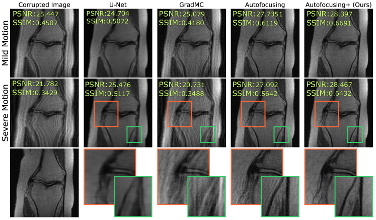
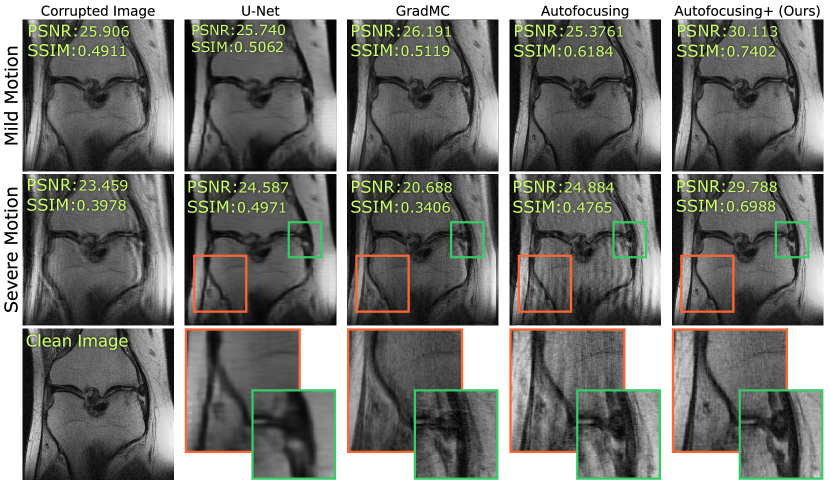
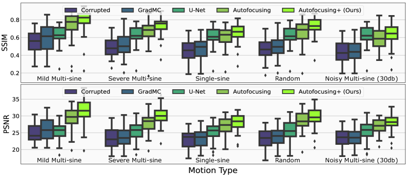
The comparison between the state-of-the-art (SOTA) optimization- and deep learning-based algorithms is shown in Fig. 3 for mild and severe motion corruptions. The validation of our method was performed with all three types of motion trajectories shown in Fig. 2. A full comparison of the trajectories is presented in Fig. 4, suggesting that the technique is functional for each of them, even the random one. We refer to Supplementary material for all four quality metrics and each motion trajectory (Table LABEL:s:all_metrics), while presenting only selected metrics herein for brevity, with the focus on the harmonic corruption as the most realistic [13].

Figure 4: Mild corruption demotion via different methods. 3T scans and synthetic noise. Autofocusing+ differs from Autofocusing for all data significantly (max p-value <10^-5).

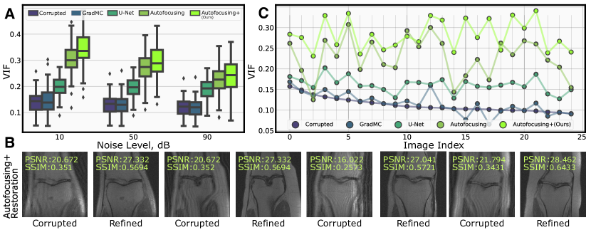
Resilience to Noise. The demotion methods have to be resilient to noise (e.g., electronic [4]) and abrupt fluctuations in the detail of an anatomic structure (e.g., when the ligaments of the joint appear next to the motion artifact). These cases are thoroughly studied in Fig. 5, where either classic optimization or deep learning methods sometimes fail to function. On the opposite, Autofocusing+ is consistent and robust on all images, showing resilience to the strongest noise levels (90 dB). In the synthetic noise experiments, the noise is modeled as Gaussian distribution $\mathcal{N}(\mu,\sigma^{2})$ added to the signal in k-space: $Y^{\prime}=Y+\mathcal{N}(\mu,\sigma^{2})$ [18], where $Y^{\prime}$ is a noise-corrupted spectrum, $\mu$ is the mean, and $\sigma$ is the standard deviation of the noise.

We also validated our algorithm on a real-noise data subset, a part of fastMRI acquired at 1T, where the SNR and the contrast are visually sub-optimal (the factual noise level is unknown). Although all methods fluctuate more severely than in the case of synthetic noise, the t-test confirms that our algorithm still outperforms the second best method (classic Autofocusing) with statistical significance (max p-value <0.0047).

Figure 5: Demotion results for harmonic motion corruption and real noise (1T scans). A. Performance for different noise levels (max p-value <0.0047). B. Example of real noisy images restored by Autofocusing+. C. Performance of all methods on 25 random images in the real-noise dataset. In some cases, classic Autofocusing fails to restore the image (e.g., image #2, #14, and #17), whereas Autofocusing+ handles the demotion.

5 Discussion

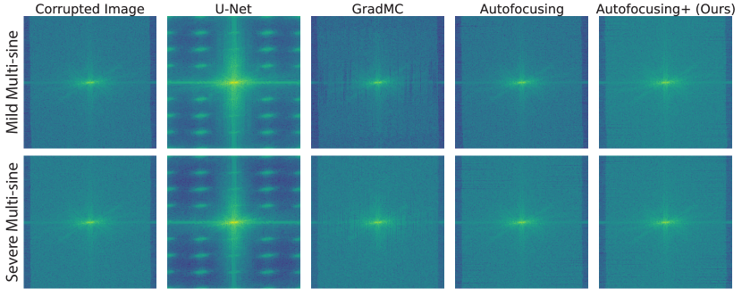
As can be seen in Figs. 4 and 5, Autofocusing+ always outperforms the SOTA models for all four metrics, all noise levels, and all motion trajectories. This affirms that the addition of neural network helps to regularize the optimization problem and improves the performance of the baseline Autofocusing method. Even visually (Fig.5(C)), Autofocusing+ succeeds in the cases where the classic optimization alone fails to refine the detail and even introduces new artifacts. We observe that such new artifacts correspond to abrupt variation of pixel intensity in the anatomic detail, where the structure ‘couples’ with the motion artifacts. The use of the neural network, however, extracts prior knowledge for the image quality measure and eliminates the issue, making the reconstruction stable and the image well-refined.

The evaluation of the reconstructed knee images for mild motion harmonic trajectories in Fig. 3 and Fig. 6 reveals only subtle differences in the performance of various methods. However, the severe corruption makes the classical optimization-based approaches inapt for removing the artifacts, whereas Autofocusing+ refines image detail, making the fine structure acceptable visually and leaving the uniform regions intact. According to Fig.5, Autofocusing+ is also efficient in the demotion task in the presence of noise, being functional both for high levels of added noise and for real low-SNR noisy MRI scans.

It can also be noticed that a simple deblurring with a stand-alone U-Net yields approximately the same consistent output for different noise levels and the strengths of motion corruption (Table LABEL:s:all_metrics in Supplementary material), learning to ‘smooth out’ the motion artefact patterns instead of fixing them [28, 22]. This results in an irreversible loss of the fine tissue structure, making the use of optimization-based demotion methods more justified and preferred in practice.

Hence, our method takes the best of both worlds: the optimization-based routine iteratively performs the blind demotion with interpretable measure of the image detail and the deep learning-based prior helps to penalize for unrealistic restorations. The latter is especially useful in practice as it helps prevent the emergence of new artifacts, sometimes induced by neural networks in MRI reconstructions [3].

Limitations. Similarly to other synthetic motion works [5, 15, 21], a Cartesian sampling with 2D in-plane motions in the phase encoding direction was assumed. Elastic movements (e.g., compression and stretching in the soft tissues [8]) were beyond the scope of our work and should be revisited, following, e.g., [35].

Stemming from the baseline Autofocusing, and similarly to other optimization-based methods, there is room to improve the inference time of Autofocusing+ which takes 7–9 minutes to process a batch of 10 images. Parallel computing and the pertinent efficient acceleration of the gradients and the Fourier transforms [27] should work well and will be the subject of future work. Likewise, the study of different neural network architectures should be conducted.

5.0.1 Conclusion.

In this work, we presented Autofocusing+, a new deep learning-based regularization method to enhance the classic optimization algorithm for compensating the corruption caused by the subject’s motion. The blind demotion routine uses the regularizer as an image prior penalizing for unrealistic restorations and improving the reconstruction quality. We validated the method on three models of motion trajectories, using synthetic and real noisy data, showing resilience to noise and anatomic structure variation and outperforming the SOTA demotion methods.

6 Supplementary

Table S1: Demotion results on validation datasets for various motion trajectories, noise inputs and methods.

Motion Type	Method	PSNR	SSIM	VIF	MS-SSIM
Harmonic Mild	Corrupted	24.98 $\pm$ 2.60	0.554 $\pm$ 0.11	0.186 $\pm$ 0.06	0.873 $\pm$ 0.05
	GradMC	26.06 $\pm$ 3.23	0.595 $\pm$ 0.15	0.216 $\pm$ 0.09	0.895 $\pm$ 0.06
	U-Net	25.51 $\pm$ 2.48	0.629 $\pm$ 0.09	0.196 $\pm$ 0.04	0.890 $\pm$ 0.03
	Autofocusing	29.46 $\pm$ 3.02	0.740 $\pm$ 0.14	0.373 $\pm$ 0.09	0.963 $\pm$ 0.03
	Autofocusing+(Ours)	31.46 $\pm$ 3.36	0.792 $\pm$ 0.13	0.407 $\pm$ 0.10	0.972 $\pm$ 0.03
Harmonic Severe	Corrupted	23.14 $\pm$ 2.75	0.486 $\pm$ 0.10	0.142 $\pm$ 0.04	0.804 $\pm$ 0.06
	GradMC	23.71 $\pm$ 2.81	0.512 $\pm$ 0.12	0.148 $\pm$ 0.06	0.819 $\pm$ 0.07
	U-Net	25.57 $\pm$ 2.68	0.626 $\pm$ 0.09	0.195 $\pm$ 0.04	0.889 $\pm$ 0.03
	Autofocusing	27.91 $\pm$ 2.55	0.664 $\pm$ 0.12	0.305 $\pm$ 0.06	0.946 $\pm$ 0.03
	Autofocusing+(Ours)	30.08 $\pm$ 2.56	0.735 $\pm$ 0.09	0.349 $\pm$ 0.06	0.964 $\pm$ 0.02
Single-sine	Corrupted	22.90 $\pm$ 2.57	0.458 $\pm$ 0.10	0.132 $\pm$ 0.03	0.780 $\pm$ 0.05
	GradMC	23.33 $\pm$ 2.48	0.482 $\pm$ 0.10	0.136 $\pm$ 0.04	0.793 $\pm$ 0.06
	U-Net	25.27 $\pm$ 2.65	0.613 $\pm$ 0.09	0.183 $\pm$ 0.03	0.879 $\pm$ 0.03
	Autofocusing	27.27 $\pm$ 2.30	0.608 $\pm$ 0.10	0.261 $\pm$ 0.04	0.924 $\pm$ 0.03
	Autofocusing+(Ours)	28.15 $\pm$ 2.48	0.653 $\pm$ 0.10	0.285 $\pm$ 0.05	0.939 $\pm$ 0.03
Random	Corrupted	23.26 $\pm$ 2.68	0.468 $\pm$ 0.10	0.136 $\pm$ 0.04	0.786 $\pm$ 0.06
	GradMC	23.89 $\pm$ 2.75	0.501 $\pm$ 0.11	0.145 $\pm$ 0.05	0.810 $\pm$ 0.07
	U-Net	25.50 $\pm$ 2.74	0.621 $\pm$ 0.09	0.189 $\pm$ 0.04	0.884 $\pm$ 0.03
	Autofocusing	28.68 $\pm$ 2.75	0.665 $\pm$ 0.13	0.303 $\pm$ 0.07	0.942 $\pm$ 0.04
	Autofocusing+(Ours)	29.83 $\pm$ 2.94	0.723 $\pm$ 0.11	0.341 $\pm$ 0.07	0.958 $\pm$ 0.03
Harmonic with noise 30 dB	Corrupted	23.35 $\pm$ 2.66	0.440 $\pm$ 0.11	0.136 $\pm$ 0.04	0.800 $\pm$ 0.06
	GradMC	23.46 $\pm$ 2.61	0.449 $\pm$ 0.11	0.135 $\pm$ 0.04	0.802 $\pm$ 0.06
	U-Net	25.67 $\pm$ 2.70	0.625 $\pm$ 0.09	0.195 $\pm$ 0.04	0.889 $\pm$ 0.03
	Autofocusing	26.86 $\pm$ 2.13	0.586 $\pm$ 0.11	0.270 $\pm$ 0.06	0.927 $\pm$ 0.03
	Autofocusing+(Ours)	28.19 $\pm$ 2.49	0.640 $\pm$ 0.12	0.300 $\pm$ 0.06	0.942 $\pm$ 0.03
Real noisy with	Corrupted	22.81 $\pm$ 2.23	0.379 $\pm$ 0.09	0.810 $\pm$ 0.05	0.131 $\pm$ 0.03
mild harmonic	GradMC	23.28 $\pm$ 2.26	0.399 $\pm$ 0.13	0.140 $\pm$ 0.05	0.814 $\pm$ 0.07
	U-Net	23.92 $\pm$ 2.39	0.442 $\pm$ 0.08	0.148 $\pm$ 0.02	0.840 $\pm$ 0.04
	Autofocusing	26.03 $\pm$ 2.77	0.590 $\pm$ 0.15	0.271 $\pm$ 0.08	0.931 $\pm$ 0.04
	Autofocusing+(Ours)	26.97 $\pm$ 2.26	0.631 $\pm$ 0.07	0.289 $\pm$ 0.04	0.948 $\pm$ 0.02
Real noisy with	Corrupted	21.70 $\pm$ 2.15	0.328 $\pm$ 0.07	0.731 $\pm$ 0.05	0.094 $\pm$ 0.02
severe harmonic	GradMC	21.82 $\pm$ 2.19	0.332 $\pm$ 0.08	0.096 $\pm$ 0.03	0.730 $\pm$ 0.06
	U-Net	23.93 $\pm$ 2.18	0.441 $\pm$ 0.08	0.144 $\pm$ 0.02	0.836 $\pm$ 0.03
	Autofocusing	25.17 $\pm$ 2.21	0.491 $\pm$ 0.11	0.219 $\pm$ 0.05	0.899 $\pm$ 0.04
	Autofocusing+(Ours)	26.45 $\pm$ 2.19	0.579 $\pm$ 0.08	0.261 $\pm$ 0.04	0.933 $\pm$ 0.02

Figure 6: k-space of refined images.

Figure 7: Examples of the demotion performance of different methods.

References

- [1] Al-masni, M.A., Lee, S., Yi, J., Kim, S., Gho, S.M., Choi, Y.H., Kim, D.H.: Stacked u-nets with self-assisted priors towards robust correction of rigid motion artifact in brain mri. arXiv preprint arXiv:2111.06401 (2021)
- [2] Atkinson, D., Hill, D.L., Stoyle, P.N., Summers, P.E., Keevil, S.F.: Automatic correction of motion artifacts in magnetic resonance images using an entropy focus criterion. IEEE Transactions on Medical Imaging 16 (1997)
- [3] Belov, A., Stadelmann, J., Kastryulin, S., Dylov, D.V.: Towards ultrafast mri via extreme k-space undersampling and superresolution. In: International Conference on Medical Image Computing and Computer-Assisted Intervention. pp. 254–264. Springer, Cham (2021)
- [4] Brown, R.W., Cheng, Y.C.N., Haacke, E.M., Thompson, M.R., Venkatesan, R.: Magnetic resonance imaging: physical principles and sequence design. John Wiley & Sons (2014)
- [5] Duffy, B.A., Zhao, L., Sepehrband, F., Min, J., Wang, D.J., Shi, Y., Toga, A.W., Kim, H.: Retrospective motion artifact correction of structural mri images using deep learning improves the quality of cortical surface reconstructions. NeuroImage 230 (2021)
- [6] Fessler, J.A., Sutton, B.P.: Nonuniform fast fourier transforms using min-max interpolation. IEEE Transactions on Signal Processing 51 (2003)
- [7] Friston, K.J., Williams, S., Howard, R., Frackowiak, R.S., Turner, R.: Movement-related effects in fmri time-series. Magnetic Resonance in Medicine 35 (1996)
- [8] Godenschweger, F., Kägebein, U., Stucht, D., Yarach, U., Sciarra, A., Yakupov, R., Lüsebrink, F., Schulze, P., Speck, O.: Motion correction in mri of the brain. Physics in medicine & biology 61(5), R32 (2016)
- [9] Haskell, M.W., Cauley, S.F., Bilgic, B., Hossbach, J., Splitthoff, D.N., Pfeuffer, J., Setsompop, K., Wald, L.L.: Network accelerated motion estimation and reduction (namer): Convolutional neural network guided retrospective motion correction using a separable motion model. Magnetic Resonance in Medicine 82 (2019)
- [10] Havsteen, I., Ohlhues, A., Madsen, K.H., Nybing, J.D., Christensen, H., Christensen, A.: Are movement artifacts in magnetic resonance imaging a real problem?—a narrative review. Frontiers in neurology 8, 232 (2017)
- [11] Kingma, D.P., Ba, J.L.: Adam: A method for stochastic optimization (2015)
- [12] Kingma, D.P., Welling, M.: Auto-encoding variational bayes. arXiv preprint arXiv:1312.6114 (2013)
- [13] Küstner, T., Armanious, K., Yang, J., Yang, B., Schick, F., Gatidis, S.: Retrospective correction of motion-affected mr images using deep learning frameworks. Magnetic resonance in medicine 82(4), 1527–1540 (2019)
- [14] Larkin, K.G., Oldfield, M.A., Klemm, H.: Fast fourier method for the accurate rotation of sampled images. Optics communications 139(1-3), 99–106 (1997)
- [15] Loktyushin, A., Nickisch, H., Pohmann, R., Schölkopf, B.: Blind multirigid retrospective motion correction of mr images. Magnetic Resonance in Medicine 73 (2015)
- [16] Lustig, M., Donoho, D.L., Santos, J.M., Pauly, J.M.: Compressed sensing mri. IEEE signal processing magazine 25(2), 72–82 (2008)
- [17] McGee, K.P., Manduca, A., Felmlee, J.P., Riederer, S.J., Ehman, R.L.: Image metric-based correction (autocorrection) of motion effects: Analysis of image metrics. Journal of Magnetic Resonance Imaging 11 (2000)
- [18] Mohan, J., Krishnaveni, V., Guo, Y.: A survey on the magnetic resonance image denoising methods. Biomedical signal processing and control 9, 56–69 (2014)
- [19] Nehrke, K., Börnert, P.: Prospective correction of affine motion for arbitrary mr sequences on a clinical scanner. Magnetic Resonance in Medicine 54 (2005)
- [20] Nielles-Vallespin, S., et al.: In vivo diffusion tensor mri of the human heart: reproducibility of breath-hold and navigator-based approaches. Magnetic resonance in medicine 70(2), 454–465 (2013)
- [21] Oksuz, I., et al.: Deep learning using k-space based data augmentation for automated cardiac mr motion artefact detection. In: International Conference on Medical Image Computing and Computer-Assisted Intervention. pp. 250–258. Springer (2018)
- [22] Pronina, V., Kokkinos, F., Dylov, D.V., Lefkimmiatis, S.: Microscopy image restoration with deep wiener-kolmogorov filters. In: European Conference on Computer Vision. pp. 185–201. Springer, Cham (2020)
- [23] Reuter, M., et al.: Head motion during mri acquisition reduces gray matter volume and thickness estimates. NeuroImage 107 (2015)
- [24] Ronneberger, O., et al.: U-net: Convolutional networks for biomedical image segmentation. In: MICCAI 2015. pp. 234–241. Springer International Publishing, Cham (2015)
- [25] Savitzky, A., Golay, M.J.: Smoothing and differentiation of data by simplified least squares procedures. Analytical Chemistry 36 (1964)
- [26] Sheikh, H.R., Bovik, A.C.: Image information and visual quality. IEEE Transactions on Image Processing 15 (2006)
- [27] Shipitsin, V., Bespalov, I., Dylov, D.V.: Global adaptive filtering layer for computer vision. arXiv preprint arXiv:2010.01177 (2020)
- [28] Siddique, N., Paheding, S., Elkin, C.P., Devabhaktuni, V.: U-net and its variants for medical image segmentation: A review of theory and applications. IEEE Access (2021)
- [29] Sommer, K., et al.: Correction of motion artifacts using a multiscale fully convolutional neural network. American Journal of Neuroradiology 41 (2020)
- [30] Tamada, D., Kromrey, M.L., Ichikawa, S., Onishi, H., Motosugi, U.: Motion artifact reduction using a convolutional neural network for dynamic contrast enhanced mr imaging of the liver. Magnetic Resonance in Medical Sciences 19 (2020)
- [31] Wang, Z., Bovik, A.C., Sheikh, H.R., Simoncelli, E.P.: Image quality assessment: From error visibility to structural similarity. IEEE Transactions on Image Processing 13 (2004)
- [32] Wang, Z., Simoncelli, E.P., Bovik, A.C.: Multiscale structural similarity for image quality assessment. In: The Thrity-Seventh Asilomar Conference on Signals, Systems & Computers, 2003. vol. 2, pp. 1398–1402. Ieee (2003)
- [33] Wood, M.L., Henkelman, R.M.: Mr image artifacts from periodic motion. Medical Physics 12 (1985)
- [34] Yang, Z., Zhang, C., Xie, L.: Sparse mri for motion correction (2013)
- [35] Zaitsev, M., Maclaren, J., Herbst, M.: Motion artifacts in mri: A complex problem with many partial solutions (2015)
- [36] Zbontar, J., , et al.: fastmri: An open dataset and benchmarks for accelerated mri. arXiv preprint arXiv:1811.08839 (2018)
- [37] Zhang, K., Zuo, W., Chen, Y., Meng, D., Zhang, L.: Beyond a gaussian denoiser: Residual learning of deep cnn for image denoising. IEEE Transactions on Image Processing 26(7), 3142–3155 (2017)