Floquet engineering of optical nonlinearities: a quantum many-body approach

Abstract

Subjecting a physical system to a time-periodic drive can substantially modify its properties and applications. This Floquet-engineering approach has been extensively applied to a wide range of classical and quantum settings in view of designing synthetic systems with exotic properties. Considering a general class of two-mode nonlinear optical devices, we show that effective optical nonlinearities can be created by subjecting the light field to a repeated pulse sequence, which couples the two modes in a fast and time-periodic manner. The strength of these drive-induced optical nonlinearities, which include an emerging four-wave mixing, can be varied by simply adjusting the pulse sequence. This leads to topological changes in the system’s phase space, which can be detected through light intensity and phase measurements. Our proposal builds on an effective-Hamiltonian approach, which derives from a parent quantum many-body Hamiltonian describing driven interacting bosons. As a corollary, our results equally apply to Bose-Einstein condensates in driven double-well potentials, where pair tunneling effectively arises from the periodic pulse sequence. Our scheme offers a practical route to engineer and finely tune exotic nonlinearities and interactions in photonics and ultracold quantum gases.

I Introduction

Floquet engineering is a vaste and pluridisciplinary program, which consists in controlling and designing synthetic systems with time-periodic drives in view of exploring novel phenomena eckardt2017colloquium ; oka2019floquet ; rudner2020band ; weitenberg2021tailoring . This general approach concerns a wide range of physical platforms, including ultracold quantum gases eckardt2017colloquium ; weitenberg2021tailoring , solid-state materials oka2019floquet ; rudner2020band , universal quantum simulators and computers georgescu2014quantum ; altman2021quantum , mechanical salerno2016floquet and acoustical fleury2016floquet systems, and photonic devices rechtsman2013photonic ; schine2016synthetic ; roushan2017chiral ; ozawa2019topological .

More specifically, Floquet engineering can be applied to modify the band structure of lattice systems eckardt2017colloquium ; rudner2020band , generate artificial gauge fields goldman2014periodically ; aidelsburger2018artificial and design complex interaction processes rapp2012ultracold ; ajoy2013quantum ; di2014quantum ; daley2014effective ; hung2016quantum ; pieplow2018generation ; lee2018floquet ; choi2020robust ; barbiero2020bose ; dehghani2021light ; geier2021floquet . These remarkable possibilities open the door to the experimental exploration of a broad range of intriguing physical phenomena, such as high-temperature superconductivity fausti2011light ; mitrano2016possible , magnetism struck2011quantum ; struck2013engineering ; gorg2018enhancement , topological physics ozawa2019topological ; rudner2020band ; weitenberg2021tailoring , many-body localization ponte2015many ; abanin2019colloquium , chaos-assisted tunneling hensinger2001dynamical ; arnal2020chaos , and lattice gauge theories barbiero2019coupling ; schweizer2019floquet .

Floquet engineering has been particularly fruitful in the realm of photonics, where various settings and periodic-driving scenarios have been proposed and experimentally realized. In laser-written optical waveguide arrays szameit2010discrete , where waveguides can be finely modulated along the propagation direction, Floquet schemes were implemented in view of generating topological band structures rechtsman2013photonic ; mukherjee2017experimental ; maczewsky2017observation ; mukherjee2018state ; mukherjee2020observation ; mukherjee2021observation , synthetic dimensions lustig2019photonic and artificial magnetic fields mukherjee2018experimental for light; these settings led to the observation of dynamic localization longhi2006observation ; szameit2009inhibition , coherent destruction of tunneling della2007visualization and modulation-assisted tunneling mukherjee2015modulation , Floquet anomalous edge states mukherjee2017experimental ; maczewsky2017observation , disorder-induced topological states stutzer2018photonic , topological solitons mukherjee2020observation ; mukherjee2021observation , as well as Aharonov-Bohm cages mukherjee2018experimental . In the context of optical resonators, electro-optical modulators were used to resonantly couple different cavity modes and realize synthetic dimensions yuan2018synthetic ; dutt2019experimental ; dutt2020single ; balvcytis2021synthetic ; englebert2021bloch , while non-planar geometries were designed to create stroboscopic dynamics reflecting an effective magnetic field for photons schine2016synthetic . In the context of circuit-QED, time-modulated couplers connecting superconducting qubits were exploited to create artificial magnetic fields for strongly-interacting photons hopping on a lattice roushan2017chiral . Finally, drive-induced optical nonlinearities recently emerged as an exciting avenue in the context of polaritons clark2019interacting ; johansen2020multimode , insulating materials shan2021giant , and high-Q microwave cavities coupled to transmon qubits zhang2022drive .

In this work, we explore the possibility of generating effective optical nonlinearities upon subjecting a propagating light field to a repeated pulse sequence. The emergence of effective nonlinearities is investigated for a general class of two-mode nonlinear systems, described by the nonlinear Schrödinger equation, where the driving sequence corresponds to a succession of fast (linear) mode-mixing operations. This framework captures a broad range of nonlinear physical settings, including two-mode optical cavities cao2017experimental ; hill2020effects ; garbin2020asymmetric , optical waveguide couplers szameit2010discrete ; szameit2009inhibition and coupled superconducting microwave cavities roushan2017chiral , but also quantum gases trapped in double-well potentials andrews1997observation ; smerzi1997quantum and two-component Bose-Einstein condensates zibold2010classical . In fact, the periodically-driven nonlinear Schrödinger equation (or Gross-Pitaevskii equation pitaevskii2016bose ) was previously investigated in the context of driven quantum gases holthaus2001towards ; kramer2005parametric ; susanto2008effects ; lellouch2017parametric ; driben2018nonlinearity ; kidd2019quantum , and more recently, in the realm of topological photonics mukherjee2020observation ; maczewsky2020nonlinearity ; mukherjee2021observation ; mochizuki2021fate ; ivanov2021topological ; see also Refs. szameit2009inhibition ; higashikawa2018floquet ; sentef2020quantum .

Our analysis is based on a parent quantum many-body Hamiltonian, which describes two species of interacting bosons subjected to a periodic pulse sequence; see the sketch in Fig. 1. This theoretical framework captures the physics of driven nonlinear optical settings in the classical (mean-field) limit pitaevskii2016bose ; carusotto2013quantum ; cao2020reconfigurable . Specifically, we first derive an effective quantum Hamiltonian that well describes the stroboscopic dynamics of the driven parent quantum system, in the high-frequency regime of the pulse sequence goldman2014periodically ; goldman2015periodically ; bukov2015universal ; eckardt2015high ; mikami2016brillouin . From this, we then derive the effective classical equations of motion, hence revealing the effective optical nonlinearities generated by the driving sequence [Section III]. We explore the validity of both approximations (i.e. the high-frequency approximation related to the drive and the mean-field approximation associated with the classical limit) through numerical simulations of the quantum and classical dynamics, comparing the full time dynamics generated by the pulse sequence to the effective descriptions [Section IV]. As a by-product, this analysis illustrates how the effective nonlinearities can be detected through the dynamics of simple observables: the relative intensity and relative phase of the two optical modes. We then discuss how the strength of the effective optical nonlinearities can be tuned by simply adjusting the pulse sequence [Section V]. This control over drive-induced optical nonlinearities is directly reflected in the topology of the systems phase space, which can be detected through light intensity and phase measurements.

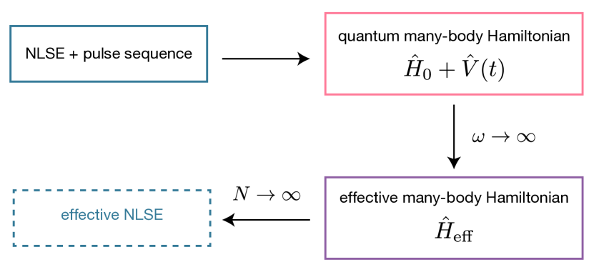
Figure 1: Schematic of the approach. We consider a general class of two-mode nonlinear systems, driven by a periodic pulse sequence and described by the nonlinear Schrödinger equation (NLSE). To analyse these settings, we introduce a parent quantum many-body Hamiltonian, $\hat{H}_{0}+\hat{V}(t)$, which describes two species of interacting bosons driven by a periodic pulse sequence. From this, we derive an effective quantum Hamiltonian $\hat{H}_{\text{eff}}$ in the high-frequency limit of the drive ($\omega\!\rightarrow\infty$). We then derive the effective nonlinear Schrödinger equation upon taking the classical limit, $N\!\rightarrow\infty$, where $N$ is the number of bosons, hence revealing the effective nonlinearities generated by the driving pulse sequence.

II The driven nonlinear system and its effective description

We consider a class of two-mode nonlinear systems, described by the (possibly coupled) nonlinear Schrödinger equations

$$i\frac{\partial\psi_{1}}{\partial t}=\left(-\gamma\frac{\partial^{2}}{\partial x^{2}}+|\psi_{1}|^{2}+\beta|\psi_{2}|^{2}\right)\psi_{1}-\frac{\Omega_{0}}{2}\psi_{2},$$

$$i\frac{\partial\psi_{2}}{\partial t}=\left(-\gamma\frac{\partial^{2}}{\partial x^{2}}+|\psi_{2}|^{2}+\beta|\psi_{1}|^{2}\right)\psi_{2}-\frac{\Omega_{0}}{2}\psi_{1}.$$ (1)

Here, $\psi_{1,2}(x,t)$ denote the complex amplitude of the fields corresponding to the modes $\sigma=1,2$; they depend on the evolution “time” $t$ and the “spatial” coordinate $x$. The focus of this work is set on the “internal” dynamics associated with the two modes, such that the “spatial” coordinate $x$ [and the related kinetic-energy term $\sim\gamma$ in Eq. (1)] does not play any role in the following. For the sake of generality, the equations of motion (1) contain two types of nonlinearities, which are generically present in optical cavities cao2017experimental ; hill2020effects ; garbin2020asymmetric : the so-called self-phase modulation and the cross-phase modulation, whose respective strengths are set by the parameter $\beta$; we have also included a static linear coupling of strength $\Omega_{0}/2$. We point out that the nonlinear equations (1) are decoupled in the limit $\Omega_{0}\!=\!\beta\!=\!0$, i.e. in the absence of linear coupling and cross-phase modulation.

While Eq. (1) naturally describes the two polarization modes of a light field propagating in a lossless cavity cao2017experimental ; hill2020effects ; garbin2020asymmetric , or light propagating in a pair of adjacent waveguides szameit2010discrete ; szameit2009inhibition , it should be noted that Eq. (1) also captures the physics of quantum gases trapped in a double well potential and two-component Bose-Einstein condensates smerzi1997quantum ; zibold2010classical .

In order to create effective nonlinearities in Eq. (1), we now include a time-periodic pulse sequence of period $T$, which mixes the two modes in a stroboscopic manner:

• Pulse $\oplus$: At times $t_{\mathfrak{n}}^{\oplus}\!=\!(T/2)\!\times\!(2\mathfrak{n}-1)$, where $\mathfrak{n}\!\in\!\mathbb{N}$, the two components undergo the mixing operation

  $$\psi_{1}\rightarrow(1/\sqrt{2})\left(\psi_{1}+i\psi_{2}\right),\,\,\psi_{2}\rightarrow(1/\sqrt{2})\left(i\psi_{1}+\psi_{2}\right).$$ (2)

• Pulse $\ominus$: at times $t_{\mathfrak{n}}^{\ominus}\!=\!T\!\times\!\mathfrak{n}$, the system undergoes the reverse operation

  $$\psi_{1}\rightarrow(1/\sqrt{2})\left(\psi_{1}-i\psi_{2}\right),\,\,\psi_{2}\rightarrow(1/\sqrt{2})\left(\psi_{2}-i\psi_{1}\right).$$ (3)

In a two-mode optical cavity cao2017experimental ; hill2020effects ; garbin2020asymmetric , these pulsed operations would correspond to a coupling between the two polarization eigenmodes of the cavity, as directly realized by means of quarter-wave plates kockaert2006fast ; kozyreff2006fast ; see the sketch in Fig. 2(a). In this case, the “time” coordinate $t$ should be interpreted as the propagation distance along the cavity fatome2021self .

More generally, when the mixing processes in Eqs. (2)-(3) cannot be directly performed by a device, they can also be realized by activating a linear coupling between the two modes, during a short pulse duration $\tau\ll T$, such that the equations of motion of the driven system can be written in the form

$$i\frac{\partial\psi_{1}}{\partial t}=\left(-\gamma\frac{\partial^{2}}{\partial x^{2}}+|\psi_{1}|^{2}+\beta|\psi_{2}|^{2}\right)\psi_{1}-\frac{\Omega(t)}{2}\psi_{2},$$ (4)

$$i\frac{\partial\psi_{2}}{\partial t}=\left(-\gamma\frac{\partial^{2}}{\partial x^{2}}+|\psi_{2}|^{2}+\beta|\psi_{1}|^{2}\right)\psi_{2}-\frac{\Omega(t)}{2}\psi_{1}.$$

Here, the function $\Omega(t)\!=\!\Omega_{0}-f_{\text{pulse}}(t)$ includes the pulse sequence defined by the function [Fig. 3(a)]

$$f_{\text{pulse}}(t) =(\pi/2\tau)\qquad t_{\mathfrak{n}}^{\oplus}-\tau\leq t\leq t_{\mathfrak{n}}^{\oplus},$$

$$=(7\pi/2\tau)\hskip 15.36429ptt_{\mathfrak{n}}^{\ominus}-\tau\leq t\leq t_{\mathfrak{n}}^{\ominus},$$

$$=0\hskip 44.10185pt\text{otherwise}.$$ (5)

To verify that the drive in Eqs. (4)-(5) indeed realizes the mixing operations in Eqs. (2)-(3), we restrict ourselves to the (linear) driving terms in the coupled Schrdinger equations (4) and we obtain the time-evolution operators corresponding to the first and second pulses, respectively:

$$\hat{U}(t_{\mathfrak{n}}^{\oplus};t_{\mathfrak{n}}^{\oplus}-\tau)=e^{-i\tau(\frac{\pi}{2\tau})(-\frac{1}{2})\hat{\sigma}_{x}}=e^{i\frac{\pi}{4}\hat{\sigma}_{x}}\equiv\hat{U}_{\text{mix}},$$ (6)

$$\hat{U}(t_{\mathfrak{n}}^{\ominus};t_{\mathfrak{n}}^{\ominus}-\tau)=e^{-i\tau(\frac{7\pi}{2\tau})(-\frac{1}{2})\hat{\sigma}_{x}}=e^{-i\frac{\pi}{4}\hat{\sigma}_{x}}=\hat{U}_{\text{mix}}^{\dagger},$$

where $\hat{\sigma}_{x}$ is the standard Pauli matrix. The operators $\hat{U}_{\text{mix}}$ and $\hat{U}_{\text{mix}}^{\dagger}$ in Eq. (6) indeed realize the mixing operations in Eqs. (2)-(3), respectively. We note that these mixing operations are reminiscent of $\pi/2$ pulses in quantum optics gardiner2014quantum ; kitagawa1993squeezed ; gross2010nonlinear . We also point out that the choice of the pulse function in Eq. (5) is not unique, e.g. the amplitude of the second pulse ($\ominus$) can be set to the value $(-\pi/2+2\pi\mathfrak{p})/\tau$, with $\mathfrak{p}\!\in\!\mathbb{Z}$, without affecting the dynamics. The advantage of the pulse function proposed in Eq. (5) is that the linear coupling does not change sign over time, which can be convenient for certain physical realizations.

In optical-waveguides settings szameit2010discrete , the two modes ($1$ and $2$) would describe light propagating in two adjacent waveguides. In this case, the pulsed linear couplings in Eqs. (4)-(5) can be realized by abruptly changing the spatial separation between the two waveguides; see Fig. 2(b) for a sketch and Refs. mukherjee2017experimental ; maczewsky2017observation ; mukherjee2020observation ; mukherjee2021observation for experimental realizations using ultrafast-laser-inscribed waveguides. Such optical-waveguides settings could benefit from the state-recycling technique of Refs. mukherjee2018state ; duncan2020synthetic , where light is re-injected into the waveguides (and possibly modified) at every roundtrip; see also Refs. kraych2019nonlinear ; kraych2019statistical ; kraych2020instabilites regarding setups based on recirculating fiber loops.

In the context of quantum gases trapped in a double well potential, the linear coupling between the two neighboring sites (orbitals) can be activated in a pulsed manner through a dynamical variation of the potential barrier schumm2005bose ; see also Ref. gross2010nonlinear , where fast $\pi/2$ pulses were implemented in a two-component Bose-Einstein condensate.

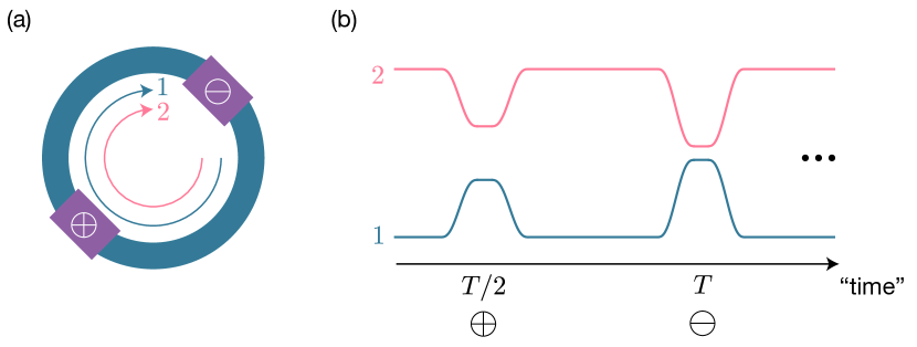
Figure 2: Two possible realizations in optics: (a) Two modes in an optical ring cavity ($1$ and $2$), repeatedly undergoing mixing operations ($\oplus$ and $\ominus$) along the ring. These operations correspond to a coupling between the two polarization eigenmodes of the cavity, as realized by means of quarter-wave plates; see Eqs. (2)-(3). (b) Two optical waveguides ($1$ and $2$) with modulated inter-waveguide separation, realizing a “time-periodic” linear coupling between the two optical modes [Eq. (4)]. In both cases, the “time” coordinate corresponds to the propagation direction szameit2010discrete ; fatome2021self .

In the limit of a fast pulse sequence, namely, when the period of the drive $T\ll T_{\text{eff}}$ is much smaller than the effective “time” scale of the system (to be discussed below), the stroboscopic time-evolution of the nonlinear system is found to be well described by the effective equations of motion

$$i\frac{\partial\psi_{1}}{\partial t}=\left(-\gamma\frac{\partial^{2}}{\partial x^{2}}+\frac{\chi}{4}|\psi_{1}|^{2}\right)\psi_{1}-\frac{\Omega_{0}}{2}\psi_{2}-\frac{\chi}{4}\psi_{1}^{*}\psi_{2}^{2},$$

$$i\frac{\partial\psi_{2}}{\partial t}=\left(-\gamma\frac{\partial^{2}}{\partial x^{2}}+\frac{\chi}{4}|\psi_{2}|^{2}\right)\psi_{2}-\frac{\Omega_{0}}{2}\psi_{1}-\frac{\chi}{4}\psi_{2}^{*}\psi_{1}^{2},$$ (7)

where we introduced the quantity $\chi\!=\!1-\beta$, and where the system is assumed to be measured stroboscopically ($t\!=\!T\!\times\!\mathfrak{n}$, with $\mathfrak{n}\!\in\!\mathbb{N}$). Comparing Eq. (7) with the original Eq. (1), we find that the repeated mixing processes in Eqs. (2)-(3) effectively produce a new form of nonlinearity, commonly known in optics as four-wave mixing agrawal2001applications ; agrawal2012nonlinear . The drive also renormalizes the self-phase-modulation and it effectively annihilates the cross-phase modulation. We point out that the effective four-wave mixing is induced even in the limit of two initially decoupled modes ($\beta\!=\!\Omega_{0}\!=\!0$).

It is the aim of the following Sections III-IV to demonstrate the effective description displayed in Eq. (7) and to explore its regimes of validity. We then introduce an “imbalanced” pulse sequence in Section V, which allows one to tune the relative strengths of effective nonlinearities and induce topological changes in phase space. While this work sets the focus on the Floquet engineering of classical nonlinear systems, the results obtained below also apply to the quantum dynamics of driven interacting bosonic systems.

As a technical note, we point out that the mixing processes in Eqs. (2)-(3) do not modify the kinetic-energy terms in Eq. (1). For the sake of presentation, we henceforth set $\gamma\!=\!0$ (except otherwise stated), but we do keep in mind that these terms can be readily added in the description without affecting the results footnote .

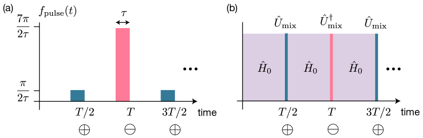
Figure 3: (a) Pulse function determining the stroboscopic activation of the linear coupling in Eqs. (4)-(5). (b) The pulse sequence associated with the time-evolution operator in Eq. (18), which involves stroboscopic mixing operations $\hat{U}_{\text{mix}}^{(\dagger)}$ separated by “free” time evolution ($\hat{H}_{0}$).

III A quantum many-body approach

Our approach consists in three successive steps [Fig. 1]:

• We introduce a parent quantum many-body Hamiltonian, whose semiclassical dynamics reproduces the time evolution of the driven nonlinear system in Eq. (4);

• Within this quantum framework, we derive the effective (Floquet) Hamiltonian that well captures the long time dynamics in the high-frequency limit ($2\pi/T\rightarrow\infty$);

• We then obtain the effective classical equations of motion from the effective quantum Hamiltonian.

The validity of this approach will then be verified in Section IV, through numerical studies of both quantum and classical dynamics.

III.1 The parent quantum many-body system

Our starting point is the quantum many-body Hamiltonian

$$\hat{H}_{0}= \frac{1}{2}\left(\hat{a}_{1}^{\dagger}\hat{a}_{1}^{\dagger}\hat{a}_{1}\hat{a}_{1}+\hat{a}_{2}^{\dagger}\hat{a}_{2}^{\dagger}\hat{a}_{2}\hat{a}_{2}\right)$$

$$+\beta\hat{a}_{1}^{\dagger}\hat{a}_{2}^{\dagger}\hat{a}_{1}\hat{a}_{2}-\frac{\Omega_{0}}{2}\left(\hat{a}_{1}^{\dagger}\hat{a}_{2}+\hat{a}_{2}^{\dagger}\hat{a}_{1}\right),$$ (8)

where $\hat{a}_{\sigma}^{\dagger}$ (resp. $\hat{a}_{\sigma}$) creates (resp. annihilates) a boson in the mode $\sigma\!=\!1,2$. These operators satisfy the bosonic commutation relations, $[\hat{a}_{\sigma},\hat{a}_{\sigma^{\prime}}^{\dagger}]=\delta_{\sigma,\sigma^{\prime}}$. The first line in Eq. (8) describes intra-mode (Hubbard) interactions, while the second line describes inter-mode (cross) interactions of strength $\beta$; the Hamiltonian also includes single-particle hopping processes of amplitude $\Omega_{0}/2$; see Fig. 4(a)-(c) for a sketch of the processes and Refs. bloch2008many ; dutta2015non . Henceforth, the Hubbard interaction strength $U\!=\!1$ sets our unit of energy, as well as our unit of time $t_{\text{unit}}\!=\!\hbar/U$.

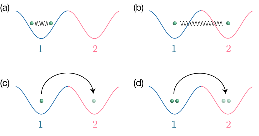
Figure 4: Processes in the Hamiltonian in Eq. (8): (a) Intra-mode (Hubbard) interactions; (b) inter-mode (cross) interactions; and (c) single-particle hopping processes. (d) The effective Hamiltonian in Eq. (30) includes pair-hopping processes, by which two interacting particles in the same mode simultaneously change mode. In this illustration, the two modes $1$ and $2$ correspond to the low-energy orbitals of a double-well potential, and the bosons are represented by green atoms.

First of all, we note that the classical equations of motion in Eq. (1) are readily obtained from Heisenberg’s equations, $d\hat{a}_{\sigma}/dt=i[\hat{H}_{0},\hat{a}_{\sigma}]$, upon taking the classical limit $\hat{a}_{1,2}\rightarrow\psi_{1,2}$; see Refs. holthaus2001towards ; carusotto2013quantum ; cao2020reconfigurable . Specifically, the self-phase modulation in Eq. (1) stems from the intra-mode (Hubbard) interaction terms in Eq. (8), while the cross-phase modulation stems from the inter-mode (cross) interaction term. Hence, this justifies the choice of Eq. (8) as a proper parent quantum Hamiltonian for our initial (non-driven) system. Note that we set $\hbar\!=\!1$ throughout this work.

In fact, for the sake of later convenience, it is instructive to derive the classical equations of motion in Eq. (1) using a different approach. Indeed, this will allow us to introduce central notions and quantities, which will be used throughout this work. Let us introduce a set of angular momentum (Schwinger) operators auerbach2012interacting , defined as

$$\hat{J}_{x}=\frac{1}{2}\left(\hat{a}_{1}^{\dagger}\hat{a}_{2}+\hat{a}_{2}^{\dagger}\hat{a}_{1}\right),\quad\hat{J}_{y}=\frac{1}{2i}\left(\hat{a}_{2}^{\dagger}\hat{a}_{1}-\hat{a}_{1}^{\dagger}\hat{a}_{2}\right),$$

$$\hat{J}_{z}=\frac{1}{2}\left(\hat{a}_{2}^{\dagger}\hat{a}_{2}-\hat{a}_{1}^{\dagger}\hat{a}_{1}\right),\quad\hat{N}=\hat{a}_{1}^{\dagger}\hat{a}_{1}+\hat{a}_{2}^{\dagger}\hat{a}_{2}.$$ (9)

These operators satisfy the spin commutation relations $[\hat{J}_{\mu},\hat{J}_{\nu}]=i\varepsilon_{\mu\nu\lambda}\hat{J}_{\lambda}$, and the operator $\hat{N}$ counts the total number of bosons in the system (assumed to be constant); note that $\hat{J}_{\mu}\!=\!\hat{\sigma}_{\mu}/2$ for a single boson ($N\!=\!1$), where $\hat{\sigma}_{x,y,z}$ denote the Pauli matrices. Using the operators in Eq. (9), the parent Hamiltonian in Eq. (8) simply reads

$$\hat{H}_{0}=\chi\hat{J}_{z}^{2}-\Omega_{0}\hat{J}_{x}+\text{constant},\qquad\chi\!=\!1-\beta,$$ (10)

and we henceforth neglect the constant terms (proportional to $\hat{N}$ and $\hat{N}^{2}$); see Appendix A. We note that the Hamiltonian in Eq. (10) has been extensively studied in the context of the bosonic Josephson effect zibold2010classical ; zibold2012classical and nuclear physics lipkin1965validity .

The equations of motion associated with Eq. (10) are readily obtained from Heisenberg’s equations

$$\frac{d\hat{J}_{z}(t)}{dt}=i[\hat{H}_{0},\hat{J}_{z}(t)]=-\Omega_{0}\hat{J}_{y}(t),$$ (11)

$$\frac{d\hat{J}_{y}(t)}{dt}=i[\hat{H}_{0},\hat{J}_{y}(t)]=\Omega_{0}\hat{J}_{z}(t)$$

$$\hskip 99.58464pt+\chi\left(\hat{J}_{z}(t)\hat{J}_{x}(t)+\hat{J}_{x}(t)\hat{J}_{z}(t)\right).$$

In order to connect Eq. (11) to the classical nonlinear Schrödinger equation in Eq. (1), we take the classical limit and introduce the Bloch-Poincaré sphere representation $(\theta,\varphi)$ through the mapping

$$\hat{J}_{x}\rightarrow\frac{N}{2}\sqrt{1-z^{2}}\cos\varphi,\quad\hat{J}_{y}\rightarrow-\frac{N}{2}\sqrt{1-z^{2}}\sin\varphi,$$

$$\hat{J}_{z}\rightarrow-\frac{N}{2}z,\hskip 56.9055ptz=\cos\theta.$$ (12)

Injecting this into Eq. (11), one obtains the classical equations of motion

$$\dot{z}=-\Omega_{0}\sqrt{1-z^{2}}\sin\varphi,$$

$$\dot{\varphi}=N\chi z+\Omega_{0}\frac{z}{\sqrt{1-z^{2}}}\cos\varphi,$$ (13)

for the two canonical conjugate variables $z(t)$ and $\varphi(t)$ zibold2010classical ; smerzi1997quantum .

We point out that Eq. (13) is equivalent to the nonlinear Schrödinger equation in Eq. (1) upon representing the complex amplitudes $\psi_{1,2}$ on the Bloch-Poincaré sphere paraoanu2001josephson ; cao2020reconfigurable

$$\psi_{1}=\sqrt{N}\cos(\theta/2)\,e^{-i\varphi/2}=\sqrt{\frac{N}{2}+n}\,e^{-i\varphi/2},$$

$$\psi_{2}=\sqrt{N}\sin(\theta/2)\,e^{i\varphi/2}=\sqrt{\frac{N}{2}-n}\,e^{i\varphi/2},$$ (14)

where we introduced the relative phase $\varphi$ between the two modes, the relative population (or relative light intensity)

$$z=\cos\theta=\frac{2n}{N}=\left(|\psi_{1}|^{2}-|\psi_{2}|^{2}\right)/N,$$ (15)

and the total population (or total light intensity)

$$N=|\psi_{1}|^{2}+|\psi_{2}|^{2}.$$ (16)

We emphasize that the dynamics in phase space, i.e. the trajectories ($z(t),\varphi(t))$, can be simply monitored in an optical setting by measuring the light intensity and the relative phase of the two modes.

For the sake of completeness, we note that the equations of motion in Eq. (13) can be derived from Hamilton’s equation, using the classical Hamiltonian zibold2010classical ; smerzi1997quantum ; di2019nonlinear

$$\mathcal{H}_{0}(z,\varphi)=\frac{\chi N}{2}z^{2}-\Omega_{0}\sqrt{1-z^{2}}\cos\varphi.$$ (17)

The classical dynamics of the non-driven system hence relies on a competition between the “mean-field” interaction parameter $g\!=\!\chi N$ and the linear coupling $\Omega_{0}$. This competition is at the core of bifurcations and symmetry breaking in the bosonic Josephson effect zibold2010classical ; cao2017experimental ; cao2020reconfigurable .

III.2 The pulse sequence and the effective Floquet Hamiltonian

We now introduce the quantum-many-body analogue of the pulse sequence introduced in Eqs. (2)-(5). We write the time-evolution operator over one period $T$ in the form [Fig. 3(b)]

$$\hat{U}(T;0)=\hat{U}_{\text{mix}}^{\dagger}\,e^{-i\frac{T}{2}\hat{H}_{0}}\hat{U}_{\text{mix}}\,e^{-i\frac{T}{2}\hat{H}_{0}},$$ (18)

where the mixing operator is defined as

$$\hat{U}_{\text{mix}}=e^{i\frac{\pi}{2}\hat{J}_{x}}.$$ (19)

We note that this indeed corresponds to the $\pi/2$-pulse operator in Eq. (6) for a single boson ($N\!=\!1$), which is consistent with the fact that the mixing operation is a single-particle process. We also point out that we explicitly took the limit $\tau\!\rightarrow\!0$, where $\tau$ is the pulse duration; see Eq. (5).

The state of the quantum many-body system at time $t_{\mathfrak{n}}\!=\!T\!\times\!\mathfrak{n}$ is then obtained as

$$|\psi(t_{\mathfrak{n}})\rangle=\hat{U}(t_{\mathfrak{n}};0)|\psi(0)\rangle=\left(\hat{U}(T;0)\right)^{\mathfrak{n}}|\psi(0)\rangle,$$ (20)

where $|\psi(0)\rangle$ denotes the initial state of the system.

We now derive the effective (Floquet) Hamiltonian goldman2014periodically ; goldman2015periodically ; bukov2015universal , which captures the stroboscopic dynamics of the driven system, and hence, its time evolution over long time scales $t_{\mathfrak{n}}\!\gg\!T$. The effective Hamiltonian is defined through the time-evolution operator over one period kitagawa2010topological ; goldman2014periodically

$$\hat{U}(T;0)=e^{-iT\hat{H}_{\text{eff}}},$$ (21)

and it can be evaluated explicitly through a $1/\omega$-expansion, where $\omega\!=\!2\pi/T$ denotes the drive frequency; see Refs. goldman2014periodically ; goldman2015periodically ; bukov2015universal ; eckardt2015high ; mikami2016brillouin . In order to reach convergence of this infinite series expansion, we partially resum the series goldman2014periodically by splitting the time-evolution operator in Eq. (18) into two parts

$$\hat{U}(T;0)=e^{-i\frac{T}{2}\hat{H}_{1}}e^{-i\frac{T}{2}\hat{H}_{0}},$$ (22)

where we introduced the operator $\hat{H}_{1}$ defined as

$$e^{-i\frac{T}{2}\hat{H}_{1}}\equiv e^{-i\frac{\pi}{2}\hat{J}_{x}}e^{-i\frac{T}{2}\hat{H}_{0}}e^{i\frac{\pi}{2}\hat{J}_{x}}.$$ (23)

Then, assuming that $T\omega_{\text{eff}}\!\ll\!1$, where $\omega_{\text{eff}}$ is the characteristic frequency associated with the processes included in the Hamiltonians $\hat{H}_{0}$ and $\hat{H}_{1}$, we apply the Trotter approximation to Eq. (22),

$$\hat{U}(T;0)\approx e^{-i\frac{T}{2}(\hat{H}_{0}+\hat{H}_{1})},$$ (24)

from which we directly obtain the effective Hamiltonian [Eq. (21)]

$$\hat{H}_{\text{eff}}=\frac{1}{2}(\hat{H}_{0}+\hat{H}_{1})+\mathcal{O}(T).$$ (25)

Our problem of finding the effective Hamiltonian thus reduces to the calculation of $\hat{H}_{1}$ defined in Eq. (23). This step can be performed exactly, by noting that

$$\hat{H}_{1}=e^{-i\frac{\pi}{2}\hat{J}_{x}}\hat{H}_{0}\,e^{i\frac{\pi}{2}\hat{J}_{x}}=\chi\left(e^{-i\frac{\pi}{2}\hat{J}_{x}}\hat{J}_{z}^{2}\,e^{i\frac{\pi}{2}\hat{J}_{x}}\right)-\Omega_{0}\hat{J}_{x},$$ (26)

where we used the definition of $\hat{H}_{0}$ in Eq. (10). Using the Baker-Campbell-Hausdorff formula, one obtains kidd2019quantum

$$e^{-i\frac{\pi}{2}\hat{J}_{x}}\hat{J}_{z}^{2}\,e^{i\frac{\pi}{2}\hat{J}_{x}}=\hat{J}_{y}^{2},$$ (27)

such that

$$\hat{H}_{1}=\chi\hat{J}_{y}^{2}-\Omega_{0}\hat{J}_{x}.$$ (28)

The effective Hamiltonian in Eq. (25) finally reads

$$\hat{H}_{\text{eff}}=\frac{\chi}{2}(\hat{J}_{y}^{2}+\hat{J}_{z}^{2})-\Omega_{0}\hat{J}_{x}+\mathcal{O}(T).$$ (29)

From this result, we find that the Trotter approximation [Eq. (24)] is valid for a sufficiently short driving period satisfying $T\!\ll\!1/\chi$ and $T\!\ll\!1/\Omega_{0}$.

It is instructive to rewrite the effective Hamiltonian in Eq. (29) using the original bosonic operators [Appendix A],

$$\hat{H}_{\text{eff}} =\frac{\chi}{8}\left(\hat{a}_{1}^{\dagger}\hat{a}_{1}^{\dagger}\hat{a}_{1}\hat{a}_{1}+\hat{a}_{2}^{\dagger}\hat{a}_{2}^{\dagger}\hat{a}_{2}\hat{a}_{2}\right)$$

$$-\frac{\chi}{8}\left(\hat{a}_{1}^{\dagger}\hat{a}_{1}^{\dagger}\hat{a}_{2}\hat{a}_{2}+\hat{a}_{2}^{\dagger}\hat{a}_{2}^{\dagger}\hat{a}_{1}\hat{a}_{1}\right)$$

$$-\frac{\Omega_{0}}{2}\left(\hat{a}_{1}^{\dagger}\hat{a}_{2}+\hat{a}_{2}^{\dagger}\hat{a}_{1}\right)+\mathcal{O}(T).$$ (30)

A comparison with the initial Hamiltonian $\hat{H}_{0}$ in Eq. (8) indicates that the driving pulse sequence has effectively generated novel interaction terms; see the second line of Eq. (30). These “pair-hopping” terms dutta2015non ; anisimovas2015role describe processes by which two particles in mode $\sigma$ collide and end up in the other mode $\sigma^{\prime}\!\neq\!\sigma$; see Fig. 4(d). As we now discuss below, these pair-hopping terms are at the origin of the four-wave mixing nonlinearity announced in Eq. (7). We also note that the effective interaction strength is given by $U_{\text{eff}}=\chi/8\!=\!(1-\beta)/8$, where $\beta$ sets the strength of the inter-mode (cross) interaction in the initial Hamiltonian $\hat{H}_{0}$ in Eq. (8).

III.3 Effective classical equations of motion

First of all, we find that the effective nonlinear Schrödinger equation in Eq. (7) is directly obtained from the effective Hamiltonian $\hat{H}_{\text{eff}}$ in Eq. (30), using Heisenbergs equations $d\hat{a}_{\sigma}/dt=i[\hat{H}_{\text{eff}},\hat{a}_{\sigma}]$, and upon taking the classical limit $\hat{a}_{1,2}\rightarrow\psi_{1,2}$. In particular, the effective four-wave mixing in Eq. (7) originates from the effective pair-hopping terms in Eq. (30).

In analogy with Eqs. (11)-(13), we explicitly derive the classical equations of motion for the two canonical conjugate variables $z(t)$ and $\varphi(t)$, describing the relative population and phase of the two modes. Using the effective Hamiltonian in Eq. (29) and Heisenbergs equations, we find

$$\frac{d\hat{J}_{z}(t)}{dt}=i[\hat{H}_{\text{eff}},\hat{J}_{z}(t)]=-\Omega_{0}\hat{J}_{y}(t)$$

$$\hskip 99.58464pt-\frac{\chi}{2}\left(\hat{J}_{y}(t)\hat{J}_{x}(t)+\hat{J}_{x}(t)\hat{J}_{y}(t)\right),$$

$$\frac{d\hat{J}_{y}(t)}{dt}=i[\hat{H}_{\text{eff}},\hat{J}_{y}(t)]=\Omega_{0}\hat{J}_{z}(t)$$

$$\hskip 99.58464pt+\frac{\chi}{2}\left(\hat{J}_{z}(t)\hat{J}_{x}(t)+\hat{J}_{x}(t)\hat{J}_{z}(t)\right).$$

Finally, applying the Bloch-Poincaré-sphere mapping in Eq. (12), we obtain the classical equations of motion

$$\dot{z}=-\frac{\chi N}{2}(1-z^{2})\cos\varphi\sin\varphi-\Omega_{0}\sqrt{1-z^{2}}\sin\varphi,$$

$$\dot{\varphi}=\frac{\chi N}{2}z\cos^{2}\varphi+\Omega_{0}\frac{z}{\sqrt{1-z^{2}}}\cos\varphi.$$ (31)

We find that the equations of motion (31) can be derived from Hamilton’s equation, using the classical Hamiltonian

$$\mathcal{H}_{\text{eff}}(z,\varphi)=\frac{\chi N}{4}\left(z^{2}\cos^{2}\varphi+\sin^{2}\varphi\right)-\Omega_{0}\sqrt{1-z^{2}}\cos\varphi.$$ (32)

We stress that the classical equations of motion in Eq. (31) are physically equivalent to the effective nonlinear Schrödinger equation announced in Eq. (7), through the mapping provided by Eq. (14).

IV Numerical analysis

This Section aims at exploring the validity of the effective-Hamiltonian analysis developed in Section III.2 and its classical limit presented in Section III.3.

IV.1 Validating the effective quantum Hamiltonian

First, we demonstrate that the dynamics associated with the effective Hamiltonian in Eq. (30) reproduces the stroboscopic dynamics of the driven system described by Eqs. (18)-(20). To this end, we choose a coherent spin state as an initial state kitagawa1993squeezed ; zibold2012classical

$$|\psi(0)\rangle=|N,\theta,\varphi\rangle=\left(\hat{a}_{\theta,\varphi}^{\dagger}\right)^{N}|\emptyset\rangle,$$ (33)

which corresponds to a macroscopic occupation of the single-particle state,

$$|\theta,\varphi\rangle=\cos(\theta/2)|1\rangle+\sin(\theta/2)e^{i\varphi}|2\rangle,$$ (34)

defined on the Bloch sphere. Here we introduced the single-particle states $|1\rangle\!=\!\hat{a}_{1}^{\dagger}|\emptyset\rangle$ and $|2\rangle\!=\!\hat{a}_{2}^{\dagger}|\emptyset\rangle$, associated with the two modes, as well as the creation operator $\hat{a}_{\theta,\varphi}^{\dagger}|\emptyset\rangle\!=\!|\theta,\varphi\rangle$. We note that the chosen initial state in Eq. (33) behaves classically in the limit $N\!\rightarrow\!\infty$ zibold2012classical , which will be convenient for later purposes (i.e. when comparing quantum and classical dynamics).

We analyze the quantum dynamics through the evaluation of the population imbalance

$$\langle z(t_{\mathfrak{n}})\rangle=(2/N)\langle\psi(t_{\mathfrak{n}})|\hat{J}_{z}|\psi(t_{\mathfrak{n}})\rangle,\quad t_{\mathfrak{n}}\!=\!T\!\times\!\mathfrak{n},$$

where the time-evolved state $|\psi(t_{\mathfrak{n}})\rangle$ is obtained from: (i) the full time dynamics of the driven system [Eqs. (18)-(20)], and (ii) the effective Hamiltonian [Eq. (30)]. Figure 5 compares these two results for both $N\!=\!10$ and $N\!=\!50$ bosons, and the same interaction parameter $g\!=\!\chi N\!=\!5$. In both cases, one obtains that the effective description well captures the stroboscopic dynamics when the driving period is sufficiently small, $T\!\lesssim\!0.1$ in the current units [see Eq. (8)]. This analysis validates the effective Hamiltonian in Eq. (30) in the high-frequency regime.

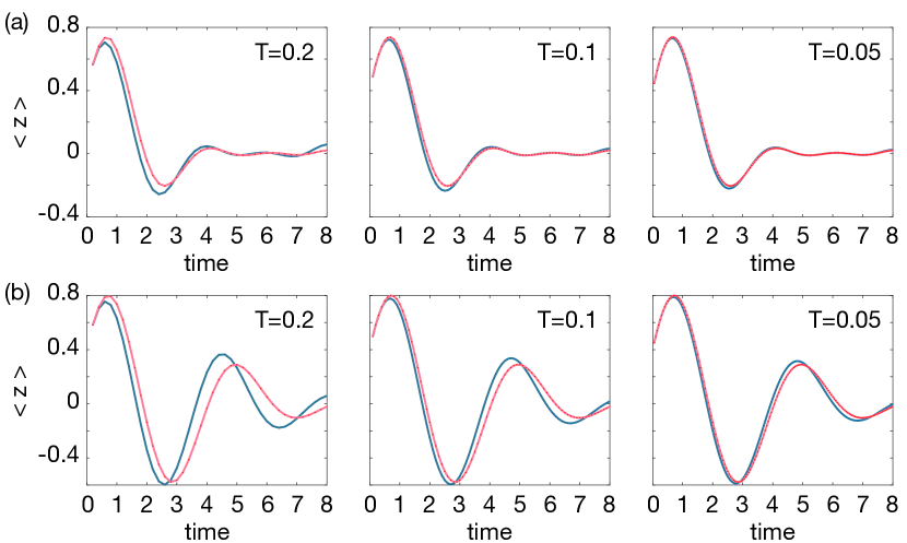
Figure 5: Population imbalance $\langle z\rangle$ as a function of time, as obtained from the quantum dynamics of the driven system (blue curve) and the effective-Hamiltonian quantum dynamics (red curve) for: (a) $N\!=\!10$ bosons and (b) $N\!=\!50$ bosons. For each case, the full time dynamics of the driven system is generated using the sequence in Eq. (18) with a period $T\!=\!0.2$, $T\!=\!0.1$ and $T\!=\!0.05$. Here the interaction parameter is set to $g\!=\!\chi N\!=\!5$ and the static linear coupling is set to $\Omega_{0}\!=\!0$; the initial coherent spin state $|N,\theta,\varphi\rangle$ corresponds to $z\!=\!\cos\theta\!=\!0.4$ and $\varphi\!=\!2.25$. In all plots, the time-evolved state is evaluated at stroboscopic times $t_{\mathfrak{n}}\!=\!T\!\times\!\mathfrak{n}$.

IV.2 The effective semiclassical dynamics

As a next step, we now show that the effective Hamiltonian $\hat{H}_{\text{eff}}$ in Eq. (30) well captures the classical dynamics generated by the equations of motion in Eq. (31). We remind that the latter classical description is associated with the Hamiltonian function $\mathcal{H}_{\text{eff}}(z,\varphi)$ displayed in Eq. (32), where $z$ and $\varphi$ describe the relative population and phase of the two modes; see Eqs. (14)-(15). The agreement between the quantum and classical descriptions is expected to be reached in the limit $N\!\rightarrow\infty$, where quantum fluctuations become negligible smerzi1997quantum ; gajda1997fluctuations ; zibold2010classical ; zibold2012classical ; carusotto2013quantum ; larre2015propagation . We also remind the reader that the classical equations of motion in Eq. (31), which are analyzed in this Section, are equivalent to the effective nonlinear Schrödinger equation in Eq. (7), through the mapping defined in Eq. (14).

First of all, let us analyze the dynamics generated by the effective classical equations of motion in Eq. (31). In order to highlight the role of nonlinearities, we hereby set the static linear coupling to $\Omega_{0}\!=\!0$. In Fig. 6, we display a few representative trajectories over the energy landscape $\mathcal{H}_{\text{eff}}(z,\varphi)$ defined in Eq. (32). These trajectories reflect the presence of two stable fixed points at $(z\!=\!0,\varphi\!=\!0)$ and $(z\!=\!0,\varphi\!=\!\pi)$. We stress that this configuration of fixed points radically differs from that associated with the non-driven system [see $\mathcal{H}_{0}(z,\varphi)$ in Eq. (17)] for the same choice of $\Omega_{0}\!=\!0$.

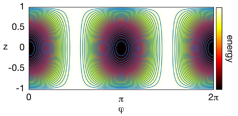
Figure 6: Energy landscape associated with the classical Hamiltonian $\mathcal{H}_{\text{eff}}(z,\varphi)$ displayed in Eq. (32), for $\Omega_{0}\!=\!0$. A few trajectories are indicated as thin blue curves (equipotential lines of the energy landscape).

We now compare these classical predictions to the quantum dynamics associated with the effective Hamiltonian $\hat{H}_{\text{eff}}$ in Eq. (30), using a coherent spin state $|N,\theta,\varphi\rangle$ as an initial condition; see Eq. (33). Figure 7 shows the trajectories $\langle z(t)\rangle$ for $N\!=\!5,10,80,170$ bosons, while keeping the “mean-field” interaction parameter $\chi N\!=\!5$ constant. From these results, we confirm that a good agreement between the effective classical and quantum descriptions is indeed obtained in the large $N$ limit.

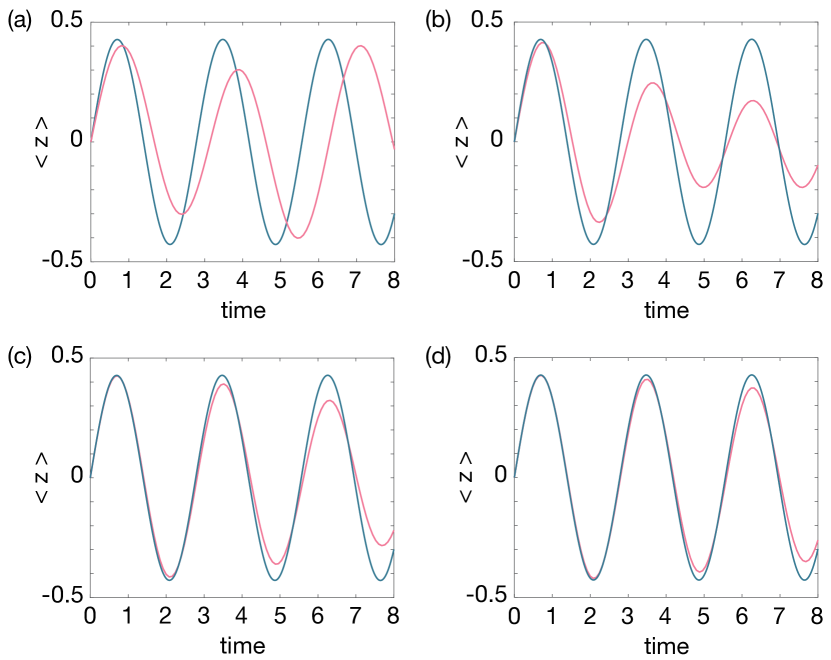
Figure 7: Population imbalance $\langle z\rangle$ as a function of time, as obtained from the effective-Hamiltonian quantum dynamics (red curve) and the effective classical equations of motion (blue curve). The number of bosons is: (a) $N\!=\!5$; (b) $N\!=\!10$; (c) $N\!=\!80$; (d) $N\!=\!170$. Here the interaction parameter is set to $g\!=\!\chi N\!=\!5$, while the static linear coupling is set to $\Omega_{0}\!=\!0$; the initial coherent spin state $|N,\theta,\varphi\rangle$ corresponds to $z\!=\!\cos\theta\!=\!0$ and $\varphi\!=\!2.7$; the same initial condition is chosen for the effective classical dynamics.

In order to further appreciate the residual deviations between the quantum and classical dynamics in the small $N$ regime, we depict the time-evolving Husimi function $Q(z,\varphi;t)$ in Fig. 8 for the case $N\!=\!80$. The Husimi function zibold2010classical ; zibold2012classical ; julia2012dynamic ; bruno2012quantum ; strobel2014fisher ; evrard2019enhanced ; nascimbene2020quantum is obtained by evaluating the squared overlap of the time-evolving state $|\psi(t)\rangle$ with the coherent spin states defined over the Bloch sphere (with same particle number $N$),

$$Q(z,\varphi;t)=|\langle N,\theta,\varphi|\psi(t)\rangle|^{2},\quad z=\cos\theta.$$ (35)

Here the state $|\psi(t)\rangle$ is evolved according to the effective Hamiltonian $\hat{H}_{\text{eff}}$ in Eq. (30), so that the evolution of the Husimi function in Fig. 8 is to be compared with the quantum dynamics displayed in Fig. 7(c) for $N\!=\!80$ bosons. The time-evolution of the Husimi function $Q(z,\varphi;t)$ shown in Fig. 8 indicates that the initial coherent spin state $|\psi(0)\rangle\!=\!|N,\theta,\varphi\rangle$ becomes substantially squeezed kitagawa1993squeezed around time $t\!\approx 3$, which also corresponds to the time around which the classical trajectory starts deviating from the effective-Hamiltonian quantum dynamics in Fig. 7(c). At later times, $t\!\approx\!12$, the state becomes oversqueezed and it exhibits Majorana stars in the Husimi distribution bruno2012quantum ; evrard2019enhanced ; nascimbene2020quantum . We find that these non-classical features are postponed to later evolution times upon increasing the number of bosons $N$ while keeping the interaction parameter $g\!=\!\chi N$ fixed. Despite these non-classical features, the center of mass of the Husimi function is found to approximately follow a classical orbit around the stable fixed point $(z\!=\!0,\varphi\!=\!\pi)$, as depicted in Fig. 6.

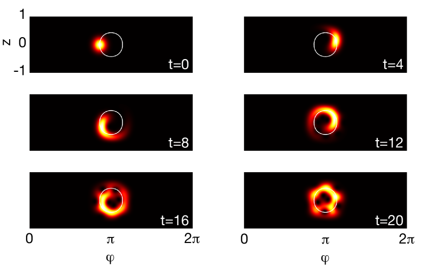
Figure 8: Time-evolving Husimi function $Q(z,\varphi;t)$ for a state $|\psi(t)\rangle$ that evolves according to the effective Hamiltonian $\hat{H}_{\text{eff}}$ in Eq. (30). Here, the number of bosons is $N\!=\!80$, and the other parameters are the same as in Fig. 7(c). The initial coherent spin state $|\psi(0)\rangle\!=\!|N,\theta,\varphi\rangle$, at $z\!=\!\cos\theta\!=\!0$ and $\varphi\!=\!2.7$, becomes substantially squeezed around time $t\!\approx\!3$, hence signaling the breakdown of its classical description. An oversqueezed state, exhibiting Majorana stars, appears around $t\!\approx\!12$. The trajectory predicted by the effective classical equations of motion [Eq. (31)] is depicted in white.

IV.3 The driven nonlinear Schrödinger equation
and its effective description

In this Section, we analyze the agreement between the classical dynamics associated with the driven nonlinear Schrödinger equation [Eqs. (4)-(5)] and the dynamics generated by the effective classical equations of motion [Eq. (31)], which derive from the Hamiltonian $\mathcal{H}_{\text{eff}}(z,\varphi)$ in Eq. (32). We remind that these effective equations of motion are equivalent to the effective nonlinear Schrödinger equation announced in Eq. (7).

In practice, we numerically solve the classical equations of motion [Eq. (13)]

$$\dot{z}=f_{\text{pulse}}(t)\sqrt{1-z^{2}}\sin\varphi,$$

$$\dot{\varphi}=N\chi z-f_{\text{pulse}}(t)\frac{z}{\sqrt{1-z^{2}}}\cos\varphi,$$ (36)

where the pulse function $f_{\text{pulse}}(t)$ is defined in Eq. (5). These equations of motion are equivalent to the driven nonlinear Schrödinger equation in Eqs. (4)-(5) through the mapping provided by Eq. (14).

The resulting dynamics are displayed in Fig. 9, together with the dynamics generated from the effective classical Hamiltonian $\mathcal{H}_{\text{eff}}(z,\varphi)$ in Eq. (32). The results in Fig. 9 confirm that the effective classical description very well captures the dynamics of the driven nonlinear system at stroboscopic times $t\!=\!t_{\mathfrak{n}}$, while a finite micromotion is observed at intermediate times $t\!\neq\!t_{\mathfrak{n}}$.

Altogether, the numerical studies presented in this Section IV validate the effective description announced in Eq. (7) [see also Sections III.2 and III.3], and hence, confirm the creation of effective interactions and nonlinearities through the repeated pulse sequence.

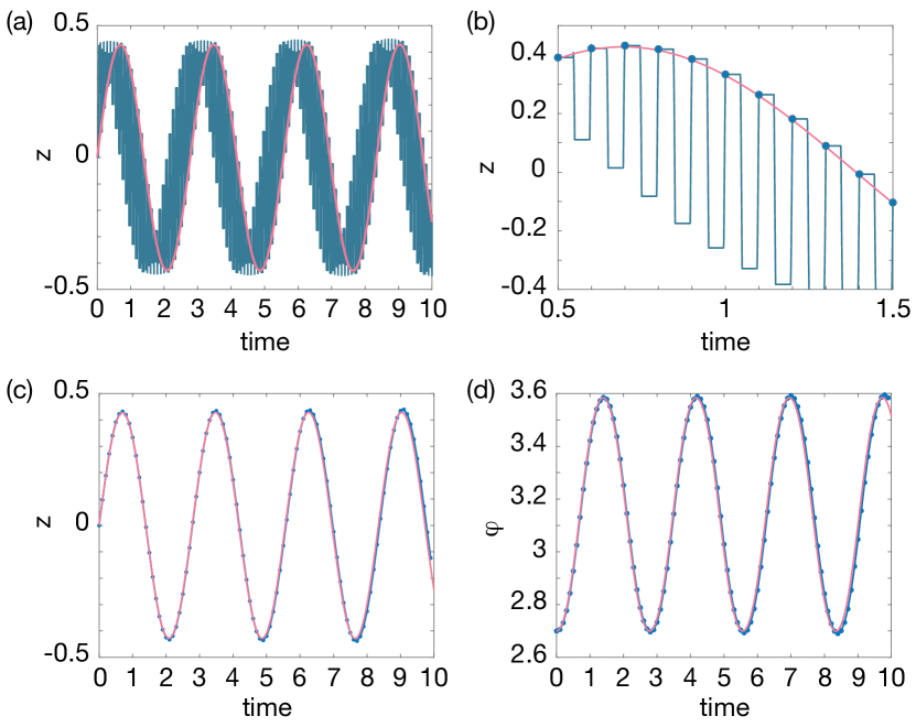
Figure 9: The driven nonlinear Schrödinger equation versus its effective description: (a) Population imbalance $z(t)$ as a function of time, as obtained from the driven nonlinear Schrödinger equation in Eq. (36) (blue curve) and from the effective classical equations of motion in Eq. (31) (red curve). (b) Zoom in the panel (a): the blue dots highlight the stroboscopic dynamics at times $t_{\mathfrak{n}}$; note the micromotion at arbitrary times $t\!\neq\!t_{\mathfrak{n}}$. (c) Stroboscopic dynamics $z(t_{\mathfrak{n}})$ obtained from the driven nonlinear Schrödinger equation (blue curve and dots), compared with the effective classical description (red curve). (d) Same as in panel (c) but for the other canonical variable $\varphi$. In all panels, the period of the drive is set to $T\!=\!0.1$ and the pulse duration to $\tau\!=\!T/20$; the interaction parameter is set to $g\!=\!\chi N\!=\!5$, while the static linear coupling is set to $\Omega_{0}\!=\!0$; the initial condition corresponds to $z\!=\!\cos\theta\!=\!0$ and $\varphi\!=\!2.7$ as in Fig. 7.

V Tuning interaction processes and classical nonlinearities

V.1 The imbalanced pulse sequence

The pulse sequence introduced in Eq. (18) corresponds to a balanced four-step sequence, with a free-evolution duration set to $T/2$ during the first and third steps of the sequence [Fig. 3(b)]. However, it is instructive to consider the “imbalanced” sequence

$$\hat{U}_{\alpha}(T;0)=\hat{U}_{\text{mix}}^{\dagger}\,e^{-i(1-\alpha)T\hat{H}_{0}}\hat{U}_{\text{mix}}\,e^{-i\alpha T\hat{H}_{0}},$$ (37)

where the parameter $\alpha$ quantifies the imbalance; note that $\alpha\!=\!1/2$ for the balanced sequence in Eq. (18). Following the approach of Section III.2, the effective Hamiltonian in Eqs. (25) and (29) is then generalized to

$$\hat{H}_{\text{eff}}^{(\alpha)} =\alpha\hat{H}_{0}+(1-\alpha)\hat{H}_{1}+\mathcal{O}(T)$$ (38)

$$=\chi\left(\alpha\hat{J}_{z}^{2}+(1-\alpha)\hat{J}_{y}^{2}\right)-\Omega_{0}\hat{J}_{x}+\mathcal{O}(T).$$

At this stage, it is important to consider two limiting cases: when $\alpha\!=\!1$, one finds $\hat{H}_{\text{eff}}\!=\!\hat{H}_{0}$, which reflects the triviality of the sequence in Eq. (37) in this case. When $\alpha\!=\!0$, one finds the effective Hamiltonian

$$\hat{H}_{\text{eff}}^{(0)}=\chi\hat{J}_{y}^{2}-\Omega_{0}\hat{J}_{x}=e^{-i\frac{\pi}{2}\hat{J}_{x}}(\hat{H}_{0})\,e^{i\frac{\pi}{2}\hat{J}_{x}},$$ (39)

which is thus strictly equivalent to the non-driven Hamiltonian $\hat{H}_{0}$ up to a unitary transformation [see Eq. (27)]: the Hamiltonians $\hat{H}_{0}$ and $\hat{H}_{\text{eff}}^{(0)}$ share the same spectrum. In fact, in the “pathological” case $\alpha\!=\!0$, the driving sequence simply generates an initial and final kick goldman2014periodically , as can be deduced by explicitly writing the time-evolving state at some arbitrary stroboscopic time $t\!=\!t_{\mathfrak{n}}$ [Eq. (20)]

$$|\psi(t_{\mathfrak{n}})\rangle =\left(\hat{U}_{\alpha=0}(T;0)\right)^{\mathfrak{n}}|\psi(0)\rangle,$$

$$=e^{-i\frac{\pi}{2}\hat{J}_{x}}e^{-it_{\mathfrak{n}}\hat{H}_{0}}e^{i\frac{\pi}{2}\hat{J}_{x}}|\psi(0)\rangle.$$ (40)

The long-time dynamics in Eq. (40) is indeed dictated by the static Hamiltonian $\hat{H}_{0}$, but it is also affected by the initial kick $e^{i\frac{\pi}{2}\hat{J}_{x}}$ and the final kick $e^{-i\frac{\pi}{2}\hat{J}_{x}}$.

Altogether, one finds that non-trivial interaction (or nonlinearity) effects are generated by driving sequences corresponding to $\hat{U}_{\alpha}(T;0)$ in Eq. (37) with $\alpha\!\neq\!0$ and $\alpha\!\neq\!1$. One indeed verifies that $\hat{H}_{\text{eff}}^{(\alpha)}$ in Eq. (38) and $\hat{H}_{0}$ do not have the same spectrum in this case.

V.2 The classical analysis: phase-space transitions and spontaneous symmetry breaking

Following Section III.3, we obtain the generalized classical equations of motion for the relative population and phase,

$$\dot{z}=-\chi N(1-\alpha)(1-z^{2})\cos\varphi\sin\varphi-\Omega_{0}\sqrt{1-z^{2}}\sin\varphi,$$

$$\dot{\varphi}=\chi Nz\left(\alpha-(1-\alpha)\sin^{2}\varphi\right)+\Omega_{0}\frac{z}{\sqrt{1-z^{2}}}\cos\varphi.$$

These equations of motion are found to derive from the classical Hamiltonian

$$\mathcal{H}_{\text{eff}}(z,\varphi;\alpha)=-\Omega_{0}\sqrt{1-z^{2}}\cos\varphi$$ (41)

$$\hskip 34.14322pt+\frac{\chi N}{2}\left(\alpha z^{2}-(1-\alpha)z^{2}\sin^{2}\varphi+(1-\alpha)\sin^{2}\varphi\right).$$

We represent the corresponding trajectories in Fig. 10, for various values of the imbalance parameter $\alpha$; in order to highlight the role of effective nonlinearities, we again set the static linear coupling to $\Omega_{0}\!=\!0$. Interestingly, the system undergoes a succession of transitions as the imbalance parameter $\alpha$ is varied, which are characterized by changes in the topology of phase space zibold2010classical : When $\alpha\!=\!0$, the system is characterized by two stable classical fixed points at $(z\!=\!0,\varphi\!=\!\pi/2)$ and $(z\!=\!0,\varphi\!=\!3\pi/2)$ [Fig. 10(a)]; increasing $\alpha$ then generates two new stable fixed points at $(z\!=\!0,\varphi\!=\!0)$ and $(z\!=\!0,\varphi\!=\!\pi)$ [Fig. 10(b)]; the two initial fixed points at $(z\!=\!0,\varphi\!=\!\pi/2)$ and $(z\!=\!0,\varphi\!=\!3\pi/2)$ then become unstable at $\alpha\!=\!0.5$ [Fig. 10(c)], giving rise to two new stable fixed points located at the poles of the Bloch-Poincaré sphere $z\!=\!\pm 1$ [Fig. 10(d)]. We note that the emerging fixed points at $z\!=\!\pm 1$ are associated with the notion of spontaneous symmetry breaking, and were previously investigated in the context of ultracold gases zibold2010classical ; zibold2012classical and in optical microcavities cao2017experimental ; cao2020reconfigurable . In the present context, the symmetry breaking occurs as soon as the $\hat{J}_{z}^{2}$ interaction term dominates over the $\hat{J}_{y}^{2}$ interaction term; see the effective Hamiltonian $\hat{H}_{\text{eff}}^{(\alpha)}$ in Eq. (38). We finally point out that the fixed points at $(z\!=\!0,\varphi\!=\!0)$ and $(z\!=\!0,\varphi\!=\!\pi)$ become unstable when $\alpha\!=\!1$ (not shown in Fig. 10).

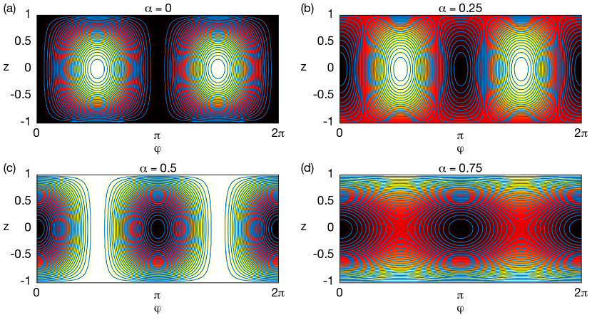
Figure 10: Energy landscape associated with the effective classical Hamiltonian $\mathcal{H}_{\text{eff}}(z,\varphi;\alpha)$ displayed in Eq. (41), for four values of the imbalance parameter: (a) $\alpha\!=\!0$, (b) $\alpha\!=\!0.25$, (c) $\alpha\!=\!0.5$ and (d) $\alpha\!=\!0.5$. A few trajectories are indicated as thin blue curves (equipotential lines of the energy landscape) for each case. The static linear coupling is set to $\Omega_{0}\!=\!0$. Note the emergence and disappearance of stable fixed points on the Bloch-Poincaré sphere, as the imbalance parameter $\alpha$ is varied.

V.3 Tunable interactions and nonlinearities

We now rewrite the generalized effective Hamiltonian in Eq. (38) in terms of the original bosonic operators [Eq. (9)],

$$\hat{H}_{\text{eff}}^{(\alpha)} =\frac{U_{1}}{2}\left(\hat{a}_{1}^{\dagger}\hat{a}_{1}^{\dagger}\hat{a}_{1}\hat{a}_{1}+\hat{a}_{2}^{\dagger}\hat{a}_{2}^{\dagger}\hat{a}_{2}\hat{a}_{2}\right)$$

$$+U_{2}\left(\hat{a}_{1}^{\dagger}\hat{a}_{2}^{\dagger}\hat{a}_{1}\hat{a}_{2}\right)$$

$$+\frac{U_{3}}{2}\left(\hat{a}_{1}^{\dagger}\hat{a}_{1}^{\dagger}\hat{a}_{2}\hat{a}_{2}+\hat{a}_{2}^{\dagger}\hat{a}_{2}^{\dagger}\hat{a}_{1}\hat{a}_{1}\right)$$

$$-\frac{\Omega_{0}}{2}\left(\hat{a}_{1}^{\dagger}\hat{a}_{2}+\hat{a}_{2}^{\dagger}\hat{a}_{1}\right)+\mathcal{O}(T),$$ (42)

where the interaction strengths are given by

$$U_{1}=\alpha(1-\beta)/2,$$

$$U_{2}=(1-2\alpha)(1-\beta)/2,$$

$$U_{3}=(\alpha-1)(1-\beta)/2.$$ (43)

From this, we find that the imbalanced pulse sequence offers an efficient method to control the strength and sign of the different interaction processes.

This picture also offers an insightful view on the transition to spontaneous symmetry breaking discussed in Section V.2: this transition, which takes place at $\alpha\!=\!1/2$, results from a competition between the intra-mode (Hubbard) interaction strength $U_{1}$ and the pair-hopping strength $U_{3}$ in Eq. (42), in the absence of linear coupling ($\Omega_{0}\!=\!0$). This is different from the transition discussed in Refs. zibold2010classical ; cao2017experimental , which involves a competition between the Hubbard interaction strength $U_{1}$ and the linear coupling $\Omega_{0}$.

Finally, in the classical limit ($N\!\rightarrow\!\infty$), the effective nonlinear Schrödinger equation associated with the imbalanced pulse sequence reads

$$i\frac{\partial\psi_{1}}{\partial t}=\left(-\gamma\frac{\partial^{2}}{\partial x^{2}}+U_{1}|\psi_{1}|^{2}+U_{2}|\psi_{2}|^{2}\right)\psi_{1}$$

$$\hskip 34.14322pt+U_{3}\psi_{1}^{*}\psi_{2}^{2}-\frac{\Omega_{0}}{2}\psi_{2},$$

$$i\frac{\partial\psi_{2}}{\partial t}=\left(-\gamma\frac{\partial^{2}}{\partial x^{2}}+U_{1}|\psi_{2}|^{2}+U_{2}|\psi_{1}|^{2}\right)\psi_{2}$$

$$\hskip 34.14322pt+U_{3}\psi_{2}^{*}\psi_{1}^{2}-\frac{\Omega_{0}}{2}\psi_{1},$$ (44)

where the three types of nonlinearities are controlled by the parameters $U_{1,2,3}$ displayed in Eq. (43). Consequently, the three types of effective nonlinearities can be tuned by adjusting the imbalanced pulse sequence.

In an optics setting, the modification of (effective) optical nonlinearities will directly manifest in the topology of phase space [Fig. 10], which can be explored by extracting the trajectories $(z(t),\varphi(t))$ through light intensity and phase measurements.

VI Concluding remarks

This work proposed a method to engineer and tune nonlinearities in two-mode optical devices, using a designed pulse sequence that couples the optical modes in a fast and periodic manner. These repeated mixing operations simply correspond to the pulsed activation of a linear coupling between the two modes, and they can thus be implemented in a broad range of two-mode nonlinear systems, ranging from microresonators cao2017experimental ; cao2020reconfigurable and two-waveguide couplers szameit2010discrete ; szameit2009inhibition to circuit-QED platforms roushan2017chiral . While we considered a generic setting that includes both self-phase and cross-phase modulations in the absence of the periodic drive [Eq. (1)], we found that effective nonlinearities emerge even when a single type of nonlinearity is present. Importantly, we demonstrated that the strength (and sign) of effective nonlinearities can be tuned by simply adjusting the pulse sequence.

To detect the emergence of drive-induced nonlinearities, we proposed to study changes in the phase space’s topology zibold2010classical , which can be explored by monitoring the dynamics of the relative intensity $z(t)$ and phase $\varphi(t)$ of the two optical modes. According to our numerical studies, these properties could already be revealed over “time” scales of the order of $5-10T$, where $T$ denotes the period of the driving sequence. This is particularly appealing for waveguide settings szameit2010discrete , where the “evolution time” associated with the propagation distance – and hence the number of driving periods – is limited. In this context, it would be interesting to combine such driving schemes with a state-recycling protocol mukherjee2018state .

While we considered a simple pulse sequence, characterized by the alternance of linear mixing operations and “free” evolution, we note that more complicated protocols and configurations could be envisaged. For instance, different types of mixing processes could be activated within each period of the drive, including nonlinear processes. Moreover, we note that similar driving schemes could be designed for $N$-mode devices, such as realized in arrays of ultrafast-laser-inscribed waveguides szameit2010discrete . In the simplest scenario, one would couple the $N$ modes by pairs, i.e. apply the pulse sequence in Eq. (18) for the neighboring modes $1\leftrightarrow 2,3\leftrightarrow 4,\dots,(N-1)\leftrightarrow N$, and then for the complementary pairs $2\leftrightarrow 3,4\leftrightarrow 5,\dots,(N-2)\leftrightarrow(N-1)$, and repeat this whole sequence in a fast and time periodic manner. In this context, it would be exciting to study the interplay of drive-induced nonlinearities and topological band structures; see for instance Ref. ivanov2021four , where edge solitons were studied in the presence of four-wave mixing.

It would also be intriguing to explore the applicability of our scheme in the context of superconducting microwave cavities chakram2021seamless , where optical nonlinearities originate from the coupling to transmon ancillas. Indeed, it was recently shown that such optical nonlinearities can be modified by applying an off-resonant drive on the transmon ancillas zhang2022drive . Moreover, in circuit-QED platforms, the linear coupling between neighboring qubits can be modulated in a time-periodic manner roushan2017chiral ; applying our pulse protocol to such settings could be used to modify the nonlinearity of the qubits, and hence, the interaction between microwave photons. In general, we anticipate that drive-induced nonlinearities, such as the effective four-wave mixing studied in this work, could be useful for nonlinear optics applications agrawal2001applications ; agrawal2012nonlinear .

Finally, we remark that the present work relies on a non-dissipative theoretical framework, where the number of bosons is conserved. Our scheme could nevertheless be applied to driven-dissipative optical devices carusotto2013quantum , such as fiber ring cavities or microresonators described by the Lugiato-Lefever equation lugiato1987spatial ; haelterman1992dissipative ; leo2010temporal ; coen2013modeling ; garbin2020asymmetric , upon treating dissipation within the Floquet analysis  higashikawa2018floquet ; schnell2020there ; schnell2021high .

Acknowledgments

This work was initiated through discussions with J. Fatome and S. Coen, who are warmly acknowledged. M. Bukov, I. Carusotto, N. R. Cooper, A. Eckardt, N. Englebert, M. Di Liberto, B. Mera, F. Petiziol and A. Schnell are also acknowledged for various discussions. The author is also very grateful to S. Coen, N. Englebert, J. Fatome, P. Kockaert and S. Mukherjee for their comments on the manuscript. The author is supported by the FRS-FNRS (Belgium), the ERC Starting Grant TopoCold and the EOS project CHEQS.

Appendix A Useful formulas

This work uses two families of operators: the bosonic operators $\hat{a}_{1}^{(\dagger)}$ and $\hat{a}_{2}^{(\dagger)}$ associated with the two modes, and which satisfy the canonical bosonic commutation relations, $[\hat{a}_{\sigma},\hat{a}_{\sigma^{\prime}}^{\dagger}]=\delta_{\sigma,\sigma^{\prime}}$, where $\sigma\!=\!1,2$; and the angular momentum (Schwinger) operators, defined as

$$\hat{J}_{x}=\frac{1}{2}\left(\hat{a}_{1}^{\dagger}\hat{a}_{2}+\hat{a}_{2}^{\dagger}\hat{a}_{1}\right),\quad\hat{J}_{y}=\frac{1}{2i}\left(\hat{a}_{2}^{\dagger}\hat{a}_{1}-\hat{a}_{1}^{\dagger}\hat{a}_{2}\right),$$

$$\hat{J}_{z}=\frac{1}{2}\left(\hat{a}_{2}^{\dagger}\hat{a}_{2}-\hat{a}_{1}^{\dagger}\hat{a}_{1}\right),\quad\hat{N}=\hat{a}_{1}^{\dagger}\hat{a}_{1}+\hat{a}_{2}^{\dagger}\hat{a}_{2}.$$ (45)

These operators satisfy the spin commutation relations $[\hat{J}_{\mu},\hat{J}_{\nu}]=i\varepsilon_{\mu\nu\lambda}\hat{J}_{\lambda}$, and the operator $\hat{N}$ counts the total number of bosons in the system (assumed to be constant).

In view of expressing interaction processes with Schwinger operators, it is useful to note that

$$\hat{J}_{z}^{2}=\frac{1}{4}\left(\hat{a}_{1}^{\dagger}\hat{a}_{1}^{\dagger}\hat{a}_{1}\hat{a}_{1}+\hat{a}_{2}^{\dagger}\hat{a}_{2}^{\dagger}\hat{a}_{2}\hat{a}_{2}-2\hat{a}_{1}^{\dagger}\hat{a}_{2}^{\dagger}\hat{a}_{1}\hat{a}_{2}+\hat{N}\right),$$

$$\hat{J}_{y}^{2}=\frac{1}{4}\left(2\hat{a}_{1}^{\dagger}\hat{a}_{2}^{\dagger}\hat{a}_{1}\hat{a}_{2}-\hat{a}_{1}^{\dagger}\hat{a}_{1}^{\dagger}\hat{a}_{2}\hat{a}_{2}-\hat{a}_{2}^{\dagger}\hat{a}_{2}^{\dagger}\hat{a}_{1}\hat{a}_{1}+\hat{N}\right),$$

$$\hat{N}^{2}=\left(\hat{a}_{1}^{\dagger}\hat{a}_{1}^{\dagger}\hat{a}_{1}\hat{a}_{1}+\hat{a}_{2}^{\dagger}\hat{a}_{2}^{\dagger}\hat{a}_{2}\hat{a}_{2}+2\hat{a}_{1}^{\dagger}\hat{a}_{2}^{\dagger}\hat{a}_{1}\hat{a}_{2}+\hat{N}\right).$$ (46)

Hence, both $\hat{J}_{z}^{2}$ and $\hat{N}^{2}$ contain intra-mode (Hubbard) and inter-mode (cross) interactions, while $\hat{J}_{y}^{2}$ contains a combination of inter-mode interactions and pair-hopping processes [Fig. 4]. We point out that $\hat{J}_{z}^{2}$ is related to $\hat{J}_{y}^{2}$ through a unitary transformation; see Eq. (27).

From Eq. (46), we can express the intra-mode (Hubbard) interaction terms as

$$\frac{1}{2}\left(\hat{a}_{1}^{\dagger}\hat{a}_{1}^{\dagger}\hat{a}_{1}\hat{a}_{1}+\hat{a}_{2}^{\dagger}\hat{a}_{2}^{\dagger}\hat{a}_{2}\hat{a}_{2}\right)=\hat{J}_{z}^{2}+\text{constant},$$ (47)

where the irrelevant constant term reads $\hat{N}(\hat{N}-2)/4$. Similarly, the inter-mode (cross) interaction term reads

$$\hat{a}_{1}^{\dagger}\hat{a}_{2}^{\dagger}\hat{a}_{1}\hat{a}_{2}=-\hat{J}_{z}^{2}+\text{constant},$$ (48)

with the irrelevant constant term $\hat{N}^{2}/4$. These expressions were used to derive the Hamiltonian in Eq. (10) from Eq. (8).

Finally, it is useful to note that a combination of intra-mode (Hubbard) interactions and pair-hopping processes can be expressed as

$$\hat{J}_{z}^{2}+\hat{J}_{y}^{2} =\frac{1}{4}\left(\hat{a}_{1}^{\dagger}\hat{a}_{1}^{\dagger}\hat{a}_{1}\hat{a}_{1}+\hat{a}_{2}^{\dagger}\hat{a}_{2}^{\dagger}\hat{a}_{2}\hat{a}_{2}\right)$$

$$-\frac{1}{4}\left(\hat{a}_{1}^{\dagger}\hat{a}_{1}^{\dagger}\hat{a}_{2}\hat{a}_{2}+\hat{a}_{2}^{\dagger}\hat{a}_{2}^{\dagger}\hat{a}_{1}\hat{a}_{1}\right)+\text{constant}.$$ (49)

This expression was used to derive the effective Hamiltonian in Eq. (30) from Eq. (29).

References

- (1) A. Eckardt, “Colloquium: Atomic quantum gases in periodically driven optical lattices,” Reviews of Modern Physics, vol. 89, no. 1, p. 011004, 2017.
- (2) T. Oka and S. Kitamura, “Floquet engineering of quantum materials,” Annual Review of Condensed Matter Physics, vol. 10, pp. 387–408, 2019.
- (3) M. S. Rudner and N. H. Lindner, “Band structure engineering and non-equilibrium dynamics in floquet topological insulators,” Nature reviews physics, vol. 2, no. 5, pp. 229–244, 2020.
- (4) C. Weitenberg and J. Simonet, “Tailoring quantum gases by floquet engineering,” Nature Physics, vol. 17, no. 12, pp. 1342–1348, 2021.
- (5) I. M. Georgescu, S. Ashhab, and F. Nori, “Quantum simulation,” Reviews of Modern Physics, vol. 86, no. 1, p. 153, 2014.
- (6) E. Altman, K. R. Brown, G. Carleo, L. D. Carr, E. Demler, C. Chin, B. DeMarco, S. E. Economou, M. A. Eriksson, K.-M. C. Fu, et al., “Quantum simulators: Architectures and opportunities,” PRX Quantum, vol. 2, no. 1, p. 017003, 2021.
- (7) G. Salerno, T. Ozawa, H. M. Price, and I. Carusotto, “Floquet topological system based on frequency-modulated classical coupled harmonic oscillators,” Physical Review B, vol. 93, no. 8, p. 085105, 2016.
- (8) R. Fleury, A. B. Khanikaev, and A. Alu, “Floquet topological insulators for sound,” Nature communications, vol. 7, no. 1, pp. 1–11, 2016.
- (9) M. C. Rechtsman, J. M. Zeuner, Y. Plotnik, Y. Lumer, D. Podolsky, F. Dreisow, S. Nolte, M. Segev, and A. Szameit, “Photonic floquet topological insulators,” Nature, vol. 496, no. 7444, pp. 196–200, 2013.
- (10) N. Schine, A. Ryou, A. Gromov, A. Sommer, and J. Simon, “Synthetic landau levels for photons,” Nature, vol. 534, no. 7609, pp. 671–675, 2016.
- (11) P. Roushan, C. Neill, A. Megrant, Y. Chen, R. Babbush, R. Barends, B. Campbell, Z. Chen, B. Chiaro, A. Dunsworth, et al., “Chiral ground-state currents of interacting photons in a synthetic magnetic field,” Nature Physics, vol. 13, no. 2, pp. 146–151, 2017.
- (12) T. Ozawa, H. M. Price, A. Amo, N. Goldman, M. Hafezi, L. Lu, M. C. Rechtsman, D. Schuster, J. Simon, O. Zilberberg, et al., “Topological photonics,” Reviews of Modern Physics, vol. 91, no. 1, p. 015006, 2019.
- (13) N. Goldman and J. Dalibard, “Periodically driven quantum systems: effective hamiltonians and engineered gauge fields,” Physical review X, vol. 4, no. 3, p. 031027, 2014.
- (14) M. Aidelsburger, S. Nascimbene, and N. Goldman, “Artificial gauge fields in materials and engineered systems,” Comptes Rendus Physique, vol. 19, no. 6, pp. 394–432, 2018.
- (15) Á. Rapp, X. Deng, and L. Santos, “Ultracold lattice gases with periodically modulated interactions,” Physical review letters, vol. 109, no. 20, p. 203005, 2012.
- (16) A. Ajoy and P. Cappellaro, “Quantum simulation via filtered hamiltonian engineering: Application to perfect quantum transport in spin networks,” Physical review letters, vol. 110, no. 22, p. 220503, 2013.
- (17) M. Di Liberto, C. E. Creffield, G. Japaridze, and C. M. Smith, “Quantum simulation of correlated-hopping models with fermions in optical lattices,” Physical Review A, vol. 89, no. 1, p. 013624, 2014.
- (18) A. J. Daley and J. Simon, “Effective three-body interactions via photon-assisted tunneling in an optical lattice,” Physical Review A, vol. 89, no. 5, p. 053619, 2014.
- (19) C.-L. Hung, A. González-Tudela, J. I. Cirac, and H. Kimble, “Quantum spin dynamics with pairwise-tunable, long-range interactions,” Proceedings of the National Academy of Sciences, vol. 113, no. 34, pp. E4946–E4955, 2016.
- (20) G. Pieplow, F. Sols, and C. E. Creffield, “Generation of atypical hopping and interactions by kinetic driving,” New Journal of Physics, vol. 20, no. 7, p. 073045, 2018.
- (21) C. H. Lee, W. W. Ho, B. Yang, J. Gong, and Z. Papić, “Floquet mechanism for non-abelian fractional quantum hall states,” Physical review letters, vol. 121, no. 23, p. 237401, 2018.
- (22) J. Choi, H. Zhou, H. S. Knowles, R. Landig, S. Choi, and M. D. Lukin, “Robust dynamic hamiltonian engineering of many-body spin systems,” Physical Review X, vol. 10, no. 3, p. 031002, 2020.
- (23) L. Barbiero, L. Chomaz, S. Nascimbene, and N. Goldman, “Bose-hubbard physics in synthetic dimensions from interaction trotterization,” Physical Review Research, vol. 2, no. 4, p. 043340, 2020.
- (24) H. Dehghani, M. Hafezi, and P. Ghaemi, “Light-induced topological superconductivity via floquet interaction engineering,” Physical Review Research, vol. 3, no. 2, p. 023039, 2021.
- (25) S. Geier, N. Thaicharoen, C. Hainaut, T. Franz, A. Salzinger, A. Tebben, D. Grimshandl, G. Zürn, and M. Weidemüller, “Floquet hamiltonian engineering of an isolated many-body spin system,” Science, vol. 374, no. 6571, pp. 1149–1152, 2021.
- (26) D. Fausti, R. Tobey, N. Dean, S. Kaiser, A. Dienst, M. C. Hoffmann, S. Pyon, T. Takayama, H. Takagi, and A. Cavalleri, “Light-induced superconductivity in a stripe-ordered cuprate,” science, vol. 331, no. 6014, pp. 189–191, 2011.
- (27) M. Mitrano, A. Cantaluppi, D. Nicoletti, S. Kaiser, A. Perucchi, S. Lupi, P. Di Pietro, D. Pontiroli, M. Riccò, S. R. Clark, et al., “Possible light-induced superconductivity in k3c60 at high temperature,” Nature, vol. 530, no. 7591, pp. 461–464, 2016.
- (28) J. Struck, C. Ölschläger, R. Le Targat, P. Soltan-Panahi, A. Eckardt, M. Lewenstein, P. Windpassinger, and K. Sengstock, “Quantum simulation of frustrated classical magnetism in triangular optical lattices,” Science, vol. 333, no. 6045, pp. 996–999, 2011.
- (29) J. Struck, M. Weinberg, C. Ölschläger, P. Windpassinger, J. Simonet, K. Sengstock, R. Höppner, P. Hauke, A. Eckardt, M. Lewenstein, et al., “Engineering ising-xy spin-models in a triangular lattice using tunable artificial gauge fields,” Nature Physics, vol. 9, no. 11, pp. 738–743, 2013.
- (30) F. Görg, M. Messer, K. Sandholzer, G. Jotzu, R. Desbuquois, and T. Esslinger, “Enhancement and sign change of magnetic correlations in a driven quantum many-body system,” Nature, vol. 553, no. 7689, pp. 481–485, 2018.
- (31) P. Ponte, Z. Papić, F. Huveneers, and D. A. Abanin, “Many-body localization in periodically driven systems,” Physical review letters, vol. 114, no. 14, p. 140401, 2015.
- (32) D. A. Abanin, E. Altman, I. Bloch, and M. Serbyn, “Colloquium: Many-body localization, thermalization, and entanglement,” Reviews of Modern Physics, vol. 91, no. 2, p. 021001, 2019.
- (33) W. K. Hensinger, H. Häffner, A. Browaeys, N. R. Heckenberg, K. Helmerson, C. McKenzie, G. J. Milburn, W. D. Phillips, S. L. Rolston, H. Rubinsztein-Dunlop, et al., “Dynamical tunnelling of ultracold atoms,” Nature, vol. 412, no. 6842, pp. 52–55, 2001.
- (34) M. Arnal, G. Chatelain, M. Martinez, N. Dupont, O. Giraud, D. Ullmo, B. Georgeot, G. Lemarié, J. Billy, and D. Guéry-Odelin, “Chaos-assisted tunneling resonances in a synthetic floquet superlattice,” Science advances, vol. 6, no. 38, p. eabc4886, 2020.
- (35) L. Barbiero, C. Schweizer, M. Aidelsburger, E. Demler, N. Goldman, and F. Grusdt, “Coupling ultracold matter to dynamical gauge fields in optical lattices: From flux attachment to ?2 lattice gauge theories,” Science advances, vol. 5, no. 10, p. eaav7444, 2019.
- (36) C. Schweizer, F. Grusdt, M. Berngruber, L. Barbiero, E. Demler, N. Goldman, I. Bloch, and M. Aidelsburger, “Floquet approach to lattice gauge theories with ultracold atoms in optical lattices,” Nature Physics, vol. 15, no. 11, pp. 1168–1173, 2019.
- (37) A. Szameit and S. Nolte, “Discrete optics in femtosecond-laser-written photonic structures,” Journal of Physics B: Atomic, Molecular and Optical Physics, vol. 43, no. 16, p. 163001, 2010.
- (38) S. Mukherjee, A. Spracklen, M. Valiente, E. Andersson, P. Öhberg, N. Goldman, and R. R. Thomson, “Experimental observation of anomalous topological edge modes in a slowly driven photonic lattice,” Nature communications, vol. 8, no. 1, pp. 1–7, 2017.
- (39) L. J. Maczewsky, J. M. Zeuner, S. Nolte, and A. Szameit, “Observation of photonic anomalous floquet topological insulators,” Nature communications, vol. 8, no. 1, pp. 1–7, 2017.
- (40) S. Mukherjee, H. K. Chandrasekharan, P. Öhberg, N. Goldman, and R. R. Thomson, “State-recycling and time-resolved imaging in topological photonic lattices,” Nature communications, vol. 9, no. 1, pp. 1–6, 2018.
- (41) S. Mukherjee and M. C. Rechtsman, “Observation of floquet solitons in a topological bandgap,” Science, vol. 368, no. 6493, pp. 856–859, 2020.
- (42) S. Mukherjee and M. C. Rechtsman, “Observation of unidirectional solitonlike edge states in nonlinear floquet topological insulators,” Physical Review X, vol. 11, no. 4, p. 041057, 2021.
- (43) E. Lustig, S. Weimann, Y. Plotnik, Y. Lumer, M. A. Bandres, A. Szameit, and M. Segev, “Photonic topological insulator in synthetic dimensions,” Nature, vol. 567, no. 7748, pp. 356–360, 2019.
- (44) S. Mukherjee, M. Di Liberto, P. Öhberg, R. R. Thomson, and N. Goldman, “Experimental observation of aharonov-bohm cages in photonic lattices,” Physical review letters, vol. 121, no. 7, p. 075502, 2018.
- (45) S. Longhi, M. Marangoni, M. Lobino, R. Ramponi, P. Laporta, E. Cianci, and V. Foglietti, “Observation of dynamic localization in periodically curved waveguide arrays,” Physical review letters, vol. 96, no. 24, p. 243901, 2006.
- (46) A. Szameit, Y. V. Kartashov, F. Dreisow, M. Heinrich, T. Pertsch, S. Nolte, A. Tünnermann, V. A. Vysloukh, F. Lederer, and L. Torner, “Inhibition of light tunneling in waveguide arrays,” Physical review letters, vol. 102, no. 15, p. 153901, 2009.
- (47) G. Della Valle, M. Ornigotti, E. Cianci, V. Foglietti, P. Laporta, and S. Longhi, “Visualization of coherent destruction of tunneling in an optical double well system,” Physical review letters, vol. 98, no. 26, p. 263601, 2007.
- (48) S. Mukherjee, A. Spracklen, D. Choudhury, N. Goldman, P. Öhberg, E. Andersson, and R. R. Thomson, “Modulation-assisted tunneling in laser-fabricated photonic wannier–stark ladders,” New journal of physics, vol. 17, no. 11, p. 115002, 2015.
- (49) S. Stützer, Y. Plotnik, Y. Lumer, P. Titum, N. H. Lindner, M. Segev, M. C. Rechtsman, and A. Szameit, “Photonic topological anderson insulators,” Nature, vol. 560, no. 7719, pp. 461–465, 2018.
- (50) L. Yuan, Q. Lin, M. Xiao, and S. Fan, “Synthetic dimension in photonics,” Optica, vol. 5, no. 11, pp. 1396–1405, 2018.
- (51) A. Dutt, M. Minkov, Q. Lin, L. Yuan, D. A. Miller, and S. Fan, “Experimental band structure spectroscopy along a synthetic dimension,” Nature communications, vol. 10, no. 1, pp. 1–8, 2019.
- (52) A. Dutt, Q. Lin, L. Yuan, M. Minkov, M. Xiao, and S. Fan, “A single photonic cavity with two independent physical synthetic dimensions,” Science, vol. 367, no. 6473, pp. 59–64, 2020.
- (53) A. Balčytis, T. Ozawa, Y. Ota, S. Iwamoto, J. Maeda, and T. Baba, “Synthetic dimension band structures on a si cmos photonic platform,” arXiv preprint arXiv:2105.13742, 2021.
- (54) N. Englebert, N. Goldman, M. Erkintalo, N. Mostaan, S.-P. Gorza, F. Leo, and J. Fatome, “Bloch oscillations of driven dissipative solitons in a synthetic dimension,” arXiv preprint arXiv:2112.10756, 2021.
- (55) L. W. Clark, N. Jia, N. Schine, C. Baum, A. Georgakopoulos, and J. Simon, “Interacting floquet polaritons,” Nature, vol. 571, no. 7766, pp. 532–536, 2019.
- (56) C. H. Johansen, J. Lang, A. Morales, A. Baumgärenter, T. Donner, and F. Piazza, “Multimode-polariton superradiance via floquet engineering,” arXiv preprint arXiv:2011.12309, 2020.
- (57) J.-Y. Shan, M. Ye, H. Chu, S. Lee, J.-G. Park, L. Balents, and D. Hsieh, “Giant modulation of optical nonlinearity by floquet engineering,” Nature, vol. 600, no. 7888, pp. 235–239, 2021.
- (58) Y. Zhang, J. C. Curtis, C. S. Wang, R. Schoelkopf, and S. Girvin, “Drive-induced nonlinearities of cavity modes coupled to a transmon ancilla,” Physical Review A, vol. 105, no. 2, p. 022423, 2022.
- (59) Q.-T. Cao, H. Wang, C.-H. Dong, H. Jing, R.-S. Liu, X. Chen, L. Ge, Q. Gong, and Y.-F. Xiao, “Experimental demonstration of spontaneous chirality in a nonlinear microresonator,” Physical Review Letters, vol. 118, no. 3, p. 033901, 2017.
- (60) L. Hill, G.-L. Oppo, M. T. Woodley, and P. Del’Haye, “Effects of self-and cross-phase modulation on the spontaneous symmetry breaking of light in ring resonators,” Physical Review A, vol. 101, no. 1, p. 013823, 2020.
- (61) B. Garbin, J. Fatome, G.-L. Oppo, M. Erkintalo, S. G. Murdoch, and S. Coen, “Asymmetric balance in symmetry breaking,” Physical Review Research, vol. 2, no. 2, p. 023244, 2020.
- (62) M. Andrews, C. Townsend, H.-J. Miesner, D. Durfee, D. Kurn, and W. Ketterle, “Observation of interference between two bose condensates,” Science, vol. 275, no. 5300, pp. 637–641, 1997.
- (63) A. Smerzi, S. Fantoni, S. Giovanazzi, and S. Shenoy, “Quantum coherent atomic tunneling between two trapped bose-einstein condensates,” Physical Review Letters, vol. 79, no. 25, p. 4950, 1997.
- (64) T. Zibold, E. Nicklas, C. Gross, and M. K. Oberthaler, “Classical bifurcation at the transition from rabi to josephson dynamics,” Physical review letters, vol. 105, no. 20, p. 204101, 2010.
- (65) L. Pitaevskii and S. Stringari, Bose-Einstein condensation and superfluidity, vol. 164. Oxford University Press, 2016.
- (66) M. Holthaus, “Towards coherent control of a bose-einstein condensate in a double well,” Physical Review A, vol. 64, no. 1, p. 011601, 2001.
- (67) M. Krämer, C. Tozzo, and F. Dalfovo, “Parametric excitation of a bose-einstein condensate in a one-dimensional optical lattice,” Physical Review A, vol. 71, no. 6, p. 061602, 2005.
- (68) H. Susanto, P. Kevrekidis, B. Malomed, and F. K. Abdullaev, “Effects of time-periodic linear coupling on two-component bose–einstein condensates in two dimensions,” Physics Letters A, vol. 372, no. 10, pp. 1631–1638, 2008.
- (69) S. Lellouch, M. Bukov, E. Demler, and N. Goldman, “Parametric instability rates in periodically driven band systems,” Physical Review X, vol. 7, no. 2, p. 021015, 2017.
- (70) R. Driben, V. Konotop, B. Malomed, T. Meier, and A. Yulin, “Nonlinearity-induced localization in a periodically driven semidiscrete system,” Physical Review E, vol. 97, no. 6, p. 062210, 2018.
- (71) R. Kidd, M. Olsen, and J. Corney, “Quantum chaos in a bose-hubbard dimer with modulated tunneling,” Physical Review A, vol. 100, no. 1, p. 013625, 2019.
- (72) L. J. Maczewsky, M. Heinrich, M. Kremer, S. K. Ivanov, M. Ehrhardt, F. Martinez, Y. V. Kartashov, V. V. Konotop, L. Torner, D. Bauer, et al., “Nonlinearity-induced photonic topological insulator,” Science, vol. 370, no. 6517, pp. 701–704, 2020.
- (73) K. Mochizuki, K. Mizuta, and N. Kawakami, “Fate of topological edge states in disordered periodically driven nonlinear systems,” Physical Review Research, vol. 3, no. 4, p. 043112, 2021.
- (74) S. K. Ivanov, Y. V. Kartashov, M. Heinrich, A. Szameit, L. Torner, and V. V. Konotop, “Topological dipole floquet solitons,” Physical Review A, vol. 103, no. 5, p. 053507, 2021.
- (75) S. Higashikawa, H. Fujita, and M. Sato, “Floquet engineering of classical systems,” arXiv preprint arXiv:1810.01103, 2018.
- (76) M. A. Sentef, J. Li, F. Künzel, and M. Eckstein, “Quantum to classical crossover of floquet engineering in correlated quantum systems,” Physical Review Research, vol. 2, no. 3, p. 033033, 2020.
- (77) I. Carusotto and C. Ciuti, “Quantum fluids of light,” Reviews of Modern Physics, vol. 85, no. 1, p. 299, 2013.
- (78) Q.-T. Cao, R. Liu, H. Wang, Y.-K. Lu, C.-W. Qiu, S. Rotter, Q. Gong, and Y.-F. Xiao, “Reconfigurable symmetry-broken laser in a symmetric microcavity,” Nature communications, vol. 11, no. 1, pp. 1–7, 2020.
- (79) N. Goldman, J. Dalibard, M. Aidelsburger, and N. R. Cooper, “Periodically driven quantum matter: The case of resonant modulations,” Physical Review A, vol. 91, no. 3, p. 033632, 2015.
- (80) M. Bukov, L. D’Alessio, and A. Polkovnikov, “Universal high-frequency behavior of periodically driven systems: from dynamical stabilization to floquet engineering,” Advances in Physics, vol. 64, no. 2, pp. 139–226, 2015.
- (81) A. Eckardt and E. Anisimovas, “High-frequency approximation for periodically driven quantum systems from a floquet-space perspective,” New journal of physics, vol. 17, no. 9, p. 093039, 2015.
- (82) T. Mikami, S. Kitamura, K. Yasuda, N. Tsuji, T. Oka, and H. Aoki, “Brillouin-wigner theory for high-frequency expansion in periodically driven systems: Application to floquet topological insulators,” Physical Review B, vol. 93, no. 14, p. 144307, 2016.
- (83) P. Kockaert, C. Cambournac, M. Haelterman, G. Kozyreff, and T. Erneux, “Fast self-pulsing through nonlinear incoherent feedback,” Optics letters, vol. 31, no. 4, pp. 495–497, 2006.
- (84) G. Kozyreff, T. Erneux, M. Haelterman, and P. Kockaert, “Fast optical self-pulsing in a temporal analog of the kerr-slice pattern-forming system,” Physical Review A, vol. 73, no. 6, p. 063815, 2006.
- (85) J. Fatome, G. Xu, B. Garbin, N. Berti, G.-L. Oppo, S. G. Murdoch, M. Erkintalo, and S. Coen, “Self-symmetrization of symmetry-breaking dynamics in passive kerr resonators,” arXiv preprint arXiv:2106.07642, 2021.
- (86) C. Gardiner and P. Zoller, The Quantum World of Ultra-Cold Atoms and Light Book I: Foundations of Quantum Optics, vol. 2. World Scientific Publishing Company, 2014.
- (87) M. Kitagawa and M. Ueda, “Squeezed spin states,” Physical Review A, vol. 47, no. 6, p. 5138, 1993.
- (88) C. Gross, T. Zibold, E. Nicklas, J. Esteve, and M. K. Oberthaler, “Nonlinear atom interferometer surpasses classical precision limit,” Nature, vol. 464, no. 7292, pp. 1165–1169, 2010.
- (89) C. W. Duncan, M. J. Hartmann, R. R. Thomson, and P. Öhberg, “Synthetic mean-field interactions in photonic lattices,” The European Physical Journal D, vol. 74, no. 5, pp. 1–7, 2020.
- (90) A. E. Kraych, P. Suret, G. El, and S. Randoux, “Nonlinear evolution of the locally induced modulational instability in fiber optics,” Physical review letters, vol. 122, no. 5, p. 054101, 2019.
- (91) A. E. Kraych, D. Agafontsev, S. Randoux, and P. Suret, “Statistical properties of the nonlinear stage of modulation instability in fiber optics,” Physical review letters, vol. 123, no. 9, p. 093902, 2019.
- (92) A. Kraych, Instabilités modulationnelles dans un anneau de recirculation fibré. PhD thesis, Lille, 2020.
- (93) T. Schumm, Bose-Einstein condensates in magnetic double well potentials. PhD thesis, 2005.
- (94) G. Agrawal, Applications of nonlinear fiber optics. Elsevier, 2001.
- (95) G. Agrawal, Nonlinear fiber optics. Elsevier, 2012.
- (96) The nonlinear Schrödinger equation in Eq. (1) assumes that the parameter is the same for both modes. If this is not the case, then Eq. (1) would display a term of the form . Since the Pauli matrix does not commute with the mixing operator in Eq. (6), this kinetic term will be modified in the effective Hamiltonian [Eq. (7)].
- (97) I. Bloch, J. Dalibard, and W. Zwerger, “Many-body physics with ultracold gases,” Reviews of modern physics, vol. 80, no. 3, p. 885, 2008.
- (98) O. Dutta, M. Gajda, P. Hauke, M. Lewenstein, D.-S. Lühmann, B. A. Malomed, T. Sowiński, and J. Zakrzewski, “Non-standard hubbard models in optical lattices: a review,” Reports on Progress in Physics, vol. 78, no. 6, p. 066001, 2015.
- (99) A. Auerbach, Interacting electrons and quantum magnetism. Springer Science & Business Media, 2012.
- (100) T. Zibold, Classical bifurcation and entanglement generation in an internal bosonic josephson junction. PhD thesis, 2012.
- (101) H. J. Lipkin, N. Meshkov, and A. Glick, “Validity of many-body approximation methods for a solvable model:(i). exact solutions and perturbation theory,” Nuclear Physics, vol. 62, no. 2, pp. 188–198, 1965.
- (102) G.-S. Paraoanu, S. Kohler, F. Sols, and A. Leggett, “The josephson plasmon as a bogoliubov quasiparticle,” Journal of Physics B: Atomic, Molecular and Optical Physics, vol. 34, no. 23, p. 4689, 2001.
- (103) M. Di Liberto, S. Mukherjee, and N. Goldman, “Nonlinear dynamics of aharonov-bohm cages,” Physical Review A, vol. 100, no. 4, p. 043829, 2019.
- (104) T. Kitagawa, E. Berg, M. Rudner, and E. Demler, “Topological characterization of periodically driven quantum systems,” Physical Review B, vol. 82, no. 23, p. 235114, 2010.
- (105) E. Anisimovas, G. Žlabys, B. M. Anderson, G. Juzeliūnas, and A. Eckardt, “Role of real-space micromotion for bosonic and fermionic floquet fractional chern insulators,” Physical Review B, vol. 91, no. 24, p. 245135, 2015.
- (106) M. Gajda and K. Rzazewski, “Fluctuations of bose-einstein condensate,” Physical review letters, vol. 78, no. 14, p. 2686, 1997.
- (107) P.-É. Larré and I. Carusotto, “Propagation of a quantum fluid of light in a cavityless nonlinear optical medium: General theory and response to quantum quenches,” Physical Review A, vol. 92, no. 4, p. 043802, 2015.
- (108) B. Julia-Diaz, T. Zibold, M. Oberthaler, M. Mele-Messeguer, J. Martorell, and A. Polls, “Dynamic generation of spin-squeezed states in bosonic josephson junctions,” Physical Review A, vol. 86, no. 2, p. 023615, 2012.
- (109) P. Bruno, “Quantum geometric phase in majoranas stellar representation: mapping onto a many-body aharonov-bohm phase,” Physical Review Letters, vol. 108, no. 24, p. 240402, 2012.
- (110) H. Strobel, W. Muessel, D. Linnemann, T. Zibold, D. B. Hume, L. Pezzè, A. Smerzi, and M. K. Oberthaler, “Fisher information and entanglement of non-gaussian spin states,” Science, vol. 345, no. 6195, pp. 424–427, 2014.
- (111) A. Evrard, V. Makhalov, T. Chalopin, L. A. Sidorenkov, J. Dalibard, R. Lopes, and S. Nascimbene, “Enhanced magnetic sensitivity with non-gaussian quantum fluctuations,” Physical review letters, vol. 122, no. 17, p. 173601, 2019.
- (112) S. Nascimbene, “Quantum-enhanced sensing and topological matter with ultracold dysprosium atoms,” 2020.
- (113) S. K. Ivanov, Y. V. Kartashov, and V. V. Konotop, “Four-wave mixing floquet topological solitons,” Optics Letters, vol. 46, no. 19, pp. 4710–4713, 2021.
- (114) S. Chakram, A. E. Oriani, R. K. Naik, A. V. Dixit, K. He, A. Agrawal, H. Kwon, and D. I. Schuster, “Seamless high-q microwave cavities for multimode circuit quantum electrodynamics,” Physical review letters, vol. 127, no. 10, p. 107701, 2021.
- (115) L. A. Lugiato and R. Lefever, “Spatial dissipative structures in passive optical systems,” Physical review letters, vol. 58, no. 21, p. 2209, 1987.
- (116) M. Haelterman, S. Trillo, and S. Wabnitz, “Dissipative modulation instability in a nonlinear dispersive ring cavity,” Optics communications, vol. 91, no. 5-6, pp. 401–407, 1992.
- (117) F. Leo, S. Coen, P. Kockaert, S.-P. Gorza, P. Emplit, and M. Haelterman, “Temporal cavity solitons in one-dimensional kerr media as bits in an all-optical buffer,” Nature Photonics, vol. 4, no. 7, pp. 471–476, 2010.
- (118) S. Coen, H. G. Randle, T. Sylvestre, and M. Erkintalo, “Modeling of octave-spanning kerr frequency combs using a generalized mean-field lugiato–lefever model,” Optics letters, vol. 38, no. 1, pp. 37–39, 2013.
- (119) A. Schnell, A. Eckardt, and S. Denisov, “Is there a floquet lindbladian?,” Physical Review B, vol. 101, no. 10, p. 100301, 2020.
- (120) A. Schnell, S. Denisov, and A. Eckardt, “High-frequency expansions for time-periodic lindblad generators,” Physical Review B, vol. 104, no. 16, p. 165414, 2021.