Non-zero $\theta_{13}$, CP-violation and Neutrinoless Double Beta Decay for Neutrino Mixing in the $A_{4}\times Z_{2}\times Z_{3}$ Flavor Symmetry Model

Abstract

We study the modification of the Altarelli-Feruglio $A_{4}$ flavor symmetry model by adding three singlet flavons $\xi^{\prime}$, $\xi^{\prime\prime}$ and $\rho$ and the model is augmented with extra $Z_{2}\times Z_{3}$ symmetry to prevent the unwanted terms in our study. The addition of these three flavons lead to two higher order corrections in the form of two perturbation parameters $\epsilon$ and $\epsilon^{\prime}$. These corrections yield the deviation from exact tri-bimaximal (TBM) neutrino mixing pattern by producing a non-zero $\theta_{13}$ and other neutrino oscillation parameters which are consistent with the latest experimental data. In both the corrections, the neutrino masses are generated via Weinberg operator. The analysis of the perturbation parameters $\epsilon$ and $\epsilon^{\prime}$, shows that normal hierarchy (NH) and inverted hierarchy (IH) for $\epsilon$ does not change much. However, as the values of $\epsilon^{\prime}$ increases, $\theta_{23}$ occupies the lower octant for NH case. We further investigate the neutrinoless double beta decay parmeter $m_{\beta\beta}$ using the parameter space of the model for both normal and inverted hierarchies of neutrino masses.

Keywords: flavor symmetry, flavons, tri-bimaximal, Weinberg operator, neutrinoless double beta decay.
PACS numbers: 12.60.-i, 14.60.Pq, 14.60.St

I Introduction

Though the particle physics experiments and observations have been successfully confirming the standard model (SM) of particle physics, the origin of flavor structure, strong CP problem, matter-antimatter asymmetry of the universe, dark matter, dark energy, non-zero tiny neutrino masses, presence of extra flavor of neutrinos, etc. are still open questions. The discovery of neutrino oscillations in 1998 by Super-Kamiokande (SK), Japan and Sudbury Neutrino Observatory (SNO), Canada are the first proof of physics beyond the standard model. In neutrino physics, we still do not know if the leptonic CP symmetry is violated or not, whether the neutrino mass eigenvalues follow normal hierarchy (NH) or inverted hierarchy (IH), if the atmospheric mixing angle $\theta_{23}$ is maximal or not, are the neutrinos of the Dirac or Majorana type, the absolute mass of the lightest neutrino flavor etc. The neutrino oscillation experiments are only sensitive to the mass squared differences $\Delta m_{ij}^{2}$, and the leptonic mixing angles $\theta_{ij}$ ($i=1,2,3$).

Neutrino physics is an experimentally driven field. It has made tremendous progress over the past few decades and attempts are underway to quantify the neutrino oscillation parameters more precisely. A few notable works in neutrino physics are placed in references King et al. (2014); King (2004); Cao et al. (2021); McDonald (2016); Kajita (2016); Vien (2020); de Salas et al. (2021); King (2017); Phong Nguyen et al. (2020); Nguyen et al. (2022).

Neutrino oscillation phenomenology is characterized by two large mixing angles, the solar angle $\theta_{12}$ and the atmospheric angle $\theta_{23}$ together with the relatively small reactor mixing angle $\theta_{13}$. In tri-bimaximal mixing (TBM), the reactor mixing angle $\theta_{13}$ is zero and the CP phase $\delta_{CP}$ is consequently undefined. However, in 2012 the Daya Bay reactor neutrino experiment ($\sin^{2}2\theta_{13}=0.089\pm 0.010\pm 0.005$) An et al. (2012) and RENO experiment $\sin^{2}2\theta_{13}=0.113\pm 0.013\pm 0.019$ Ahn et al. (2012) showed that $\theta_{13}\simeq 9^{\circ}$. Several accelerator-based long baseline neutrino oscillation experiments like MINOS Adamson et al. (2011), Double Chooz Abe et al. (2012), T2K Abe et al. (2011) also measured consistent non-zero values for $\theta_{13}$. Since TBM has been ruled out due to a non-zero reactor mixing angle, Ahn et al. (2012); Abe et al. (2012) one of the admired ways to achieve realistic mixing is through either it’s extensions or through modifications.

The widely accepted PMNS matrix encodes the mixing between the neutrino flavor eigen states ($\nu_{e}$, $\nu_{\mu}$, $\nu_{\tau}$) and their mass eigen states ($\nu_{1}$, $\nu_{2}$, $\nu_{3}$). In the three flavored paradigm, three mixing angles and one CP phase are used to parameterize this PMNS matrix , given by Equation 1.

$$U_{PMNS}=\begin{pmatrix}c_{12}c_{13}&s_{12}c_{13}&s_{13}e^{-i\delta}\\ -s_{12}c_{23}-c_{12}s_{23}s_{13}e^{i\delta}&c_{12}c_{23}-s_{12}s_{23}s_{13}e^{i\delta}&s_{23}c_{13}\\ s_{12}s_{23}-c_{12}c_{23}s_{13}e^{i\delta}&-c_{12}s_{23}-s_{12}c_{23}s_{13}e^{i\delta}&\ c_{23}c_{13}\end{pmatrix}\cdot U_{Maj}$$ (1)

where, $c_{ij}=\cos{\theta_{ij}}$, $s_{ij}=\sin{\theta_{ij}}$ such that ($i,j=1,2,3$ and $i<j$). The diagonal matrix $U_{Maj}=diag(1,e^{i\alpha},e^{i\beta})$ contains the Majorana CP phases, $\alpha$ and $\beta$, which become observable in case the neutrinos behave as Majorana particles. To show that neutrinos are Majorana particles, it require neutrino-less double beta decay to be discovered. Such kind of decays are yet to be observed. To explain these issues, symmetry would play an important role. Wendell Furry Furry (1939) considered Majorana nature of particles, to study a kinetic process which was similar to double beta disintegration without neutrino emission popularly known as neutrino-less double beta decay (NDBD) Dell’Oro et al. (2016). It can be expressed as $(A,Z)\rightarrow(A,Z+2)+2e^{-}$ which violates the lepton number by two units and creates a pair of electron, and Majorana neutrino masses are generated as electroweak symmetry is broken. The large value of the cut-off scale of lepton number violation (LNV), typically $\Lambda\sim(10^{14}-10^{15})$ GeV, is generally linked to the observed smallness of neutrino masses. Since, the neutrino mass is zero in standard modelBilenky and Giunti (2012), we need to construct a model which is beyond the standard model by adopting a new symmetry and generate non-zero neutrino mass. One such model is the effective theories, which can generate neutrino masses through Weinberg operator Weinberg (1979).

There are other frameworks beyond the standard model (BSM) that can explain the origin of neutrino masses, for examples, the Seesaw Mechanism Yanagida (1980); Minkowski (1977); Das and Das (2020); Gell-Mann (1979); Mohapatra and Senjanovic (1980); Fukuyama and Nishiura (1997); Vien et al. (2019); Yanagida (1979); Boruah and Das (2022), Supersymmetry Ma (1998), Minimal Supersymmetric Standard Model (MSSM)Csaki (1996), Next-to-Minimal Supersymmetric Standard Model (NMSSM)Ellwanger et al. (2010), String theory Ibanez and Uranga (2012), models based on extra dimensions Arkani-Hamed et al. (2001), Radiative Seesaw Mechanism Ma (2006a) and also some other models. Now, many neutrino experiments have proved beyond doubt that neutrino has tiny non-zero mass and indicate flavor mixing Aker et al. (2019); Francis (2014); Group et al. (2020); Nath and Francis (2021).

Tri-bimaximal (TBM) Harrison et al. (2002); Harrison and Scott (2002),Trimaximal (TM1/TM2) Albright and Rodejohann (2009); He and Zee (2011); Thapa and Francis (2021), Quasi-degenerate neutrino mass models Francis and Singh (2012) and Bi-large mixing patterns Boucenna et al. (2012); Chen et al. (2019); Ding et al. (2019) are examples of phenomenological neutrino mixing patterns. Also, various models based on non-abelian discrete flavor symmetries King and Luhn (2013) like $A_{4}$ Ishimori et al. (2010); Ma (2006b, 2016), $S_{3}$ Ma (2004), $S_{4}$ Bazzocchi and Merlo (2013); Ma (2005); Vien et al. (2015), $\Delta_{27}$ Ma (2008); de Medeiros Varzielas et al. (2007); Harrison et al. (2014), $\Delta_{54}$ Ishimori et al. (2009); Loualidi (2021) have been proposed to obtain tri-bimaximal mixing (TBM).

Our model is based on the Altarelli-Feruglio (A-F) $A_{4}$ discrete flavor symmetry model Altarelli and Feruglio (2006, 2005, 2010). We have extended the flavon sector of A-F model by introducing extra flavons $\xi^{\prime}$, $\xi^{\prime\prime}$ and $\rho$ which transform as $1^{\prime}$, $1^{\prime\prime}$ and 1 respectively under $A_{4}$ to get the deviation from exact TBM neutrino mixing pattern. We also introduce $Z_{2}\times Z_{3}$ symmetry in our model to prevent unwanted terms and this helps in constructing specific structure of the coupling matrices. We calculate higher dimension perturbative parameters $\epsilon$ and $\epsilon^{\prime}$ from the Lagrangian, modified the neutrino mass matrix $M_{\nu}$ and realized symmetry based studies. However, in a few similar works Brahmachari et al. (2008); Shimizu et al. (2011), they have been simply added arbitrarily perturbative terms to $M_{\nu}$ obtained from A-F model without calculations from the Lagrangian. But in these papers Karmakar and Sil (2015); King and Luhn (2011); Cooper et al. (2012); Ding and Meloni (2012), perturbative term was calculated using Type-I seesaw mechanism and departed from the tri-bimaximal mixing pattern.

Also, various efforts have been made to deviate from TBM structure by adding extra flavons in order to generate non-zero $\theta_{13}$, non-trivial CP phase, thereby explaining the experimental data. A few of them like Ahn and Kang (2012) where the author shows that non-degeneracy of the neutrino Yukawa coupling constants are the origin of the deviations from the TBM mixing and unremovable CP-phases in the neutrino Yukawa matrix give rise both low energy CP violation measurable from neutrino oscillation and high energy CP violation. In Ref. Ahn et al. (2013) the authors show that CP is spontaneously broken at high energies, after breaking of flavon symmetry by a complex vacuum expectation value of $A_{4}$ triplet and gauge singlet scalar field. In Ref. Kang et al. (2018), Dirac CP violating phase is predicted by using the experimental mixing parameters and this model is consistent with the experimental data only for the normal hierarchy of neutrino masses.

Therefore, this gives us an opportunity to analyze $M_{\nu}$ obtained through Weinberg operator in detail and study the effect of two perturbative terms $\epsilon$ and $\epsilon^{\prime}$ on neutrino oscillation parameters and NDBD parameter $m_{ee}$.

The content material of our paper is organised as follows: In section 2, we give the overview of the framework of our model by specifying the fields involved and their transformation properties under the symmetries imposed. We give two types of corrections, analyse and study the impact of these correction terms on neutrino oscillation parameters. In section 3, we do numerical analysis and study the results for the neutrino phenomenology. We finally conclude our work in section 4.

Parameters	NH (3$\sigma$)	IH (3$\sigma$)
$\Delta{m}^{2}_{21}[{10}^{-5}eV^{2}]$	$6.82\rightarrow 8.04$	$6.82\rightarrow 8.04$
$\Delta{m}^{2}_{31}[{10}^{-3}eV^{2}]$	$2.431\rightarrow 2.599$	$-2.584\rightarrow-2.413$
$\sin^{2}\theta_{12}$	$0.269\rightarrow 0.343$	$0.269\rightarrow 0.343$
$\sin^{2}\theta_{13}$	$0.02034\rightarrow 0.02430$	$0.02053\rightarrow 0.02434$
$\sin^{2}\theta_{23}$	$0.405\rightarrow 0.620$	$0.410\rightarrow 0.623$
$\delta_{CP}$	$105\rightarrow 405$	$192\rightarrow 361$

Table 1: The $3\sigma$ ranges of neutrino oscillation parameters from NuFIT 5.1 (2021) Esteban et al. (2020)

II Framework of the Model

The non-Abelian discrete symmetry group $A_{4}$ is a group of even permutations of four objects and it has 12 elements (12= $\frac{4!}{2}$). It can describe the orientation-preserving symmetry of a regular tetrahedron, so this group is also known as tetrahedron group. It can be generated by two basic permutations S and T having properties $S^{2}=T^{3}=(ST)^{3}=1$. This group representations include three one-dimensional unitary representations $1$, $1^{\prime}$, $1^{\prime\prime}$ with the generators S and T given, respectively as follows:

$$1:S=1,T=1$$

$$1^{\prime}:S=1,T=\omega^{2}$$

$$1^{\prime\prime}:S=1,T=\omega$$

and a three dimensional unitary representation with the generators

$$T=\begin{pmatrix}1&0&0\\ 0&\omega^{2}&0\\ 0&0&\omega\end{pmatrix}$$ (2)

$$S=\frac{1}{3}\begin{pmatrix}-1&2&2\\ 2&-1&2\\ 2&2&-1\end{pmatrix}$$ (3)

. Here, $\omega$ is the cubic root of unity, $\omega=exp(i2\pi)$, so that $1+\omega+\omega^{2}=0$.
The multiplication rules corresponding to the specific basis of two generators S and T are as follows:

$$1\times 1=1$$

$$1^{\prime\prime}\times 1^{\prime}=1$$

$$1^{\prime}\times\ 1^{\prime\prime}=1$$

$$3\times 3=3+3_{A}+1+1^{\prime}+1^{\prime\prime}$$

For two triplets

$$a=(a_{1},a_{2},a_{3})$$

$$b=(b_{1},b_{2},b_{3})$$

we can write

$$1\equiv(ab)=a_{1}b_{1}+a_{2}b_{3}+a_{3}b_{2}$$

$$1^{\prime}\equiv(ab)^{\prime}=a_{3}b_{3}+a_{1}b_{2}+a_{2}b_{1}$$

$$1^{\prime\prime}\equiv(ab)^{\prime\prime}=a_{2}b_{2}+a_{1}b_{3}+a_{3}b_{1}$$

Here, 1 is symmetric under the exchange of second and third elements of a and b, $1^{\prime}$ is symmetric under the exchange of the first and second elements while $1^{\prime\prime}$ is symmetric under the exchange of first and third elements.

$$3\equiv(ab)_{S}=\frac{1}{3}(2a_{1}b_{1}-a_{2}b_{3}-a_{3}b_{2},2a_{3}b_{3}-a_{1}b_{2}-a_{2}b_{1},2a_{2}b_{2}-a_{1}b_{3}-a_{3}b_{1})$$

$$3_{A}\equiv(ab)_{A}=\frac{1}{3}(a_{2}b_{3}-a_{3}b_{2},a_{1}b_{2}-a_{2}b_{1},a_{3}b_{1}-a_{1}b_{3})$$

Here 3 is symmetric and $3_{A}$ is anti-symmetric. For the symmetric case, we notice that the first element here has 2-3 exchange symmetry, the second element has 1-2 exchange symmetry and the third element has 1-3 exchange symmetry.

Field	$l$	$e^{c}$	$\mu^{c}$	$\tau^{c}$	$h_{u}$	$h_{d}$	$\Phi_{S}$	$\Phi_{T}$	$\xi$	$\xi^{\prime}$	$\xi^{\prime\prime}$	$\rho$
SU(2)	2	1	1	1	2	2	1	1	1	1	1	1
A4	3	1	$1^{\prime\prime}$	$1^{\prime}$	1	1	3	3	1	$1^{\prime}$	$1^{\prime\prime}$	1
Z3	$\omega$	$\omega^{2}$	$\omega^{2}$	$\omega^{2}$	1	1	$\omega$	1	$\omega$	$\omega$	$\omega$	1
Z2	l	1	1	1	1	1	1	1	1	1	1	-1

Table 2: Full particle content of our model.

Our model is based on the Altarelli-Feruglio $A_{4}$ model Altarelli and Feruglio (2006, 2005, 2010). We have added additional flavons $\xi^{\prime}$, $\xi^{\prime\prime}$ and $\rho$ to get the deviation from exact TBM neutrino mixing pattern. We put extra symmetry $Z_{2}\times Z_{3}$ to avoid unwanted terms. The particle content and their charge assignment under the symmetry group is given in Table 4. The left-handed lepton doublets and right-handed charged leptons ($e^{c},\mu^{c},\tau^{c}$) are assigned to triplet and singlet ($1,1^{\prime\prime},1^{\prime}$) representation under A₄ respectively and other particles transform as shown in Table-II. Here, $h_{u}$ and $h_{d}$ are the standard Higgs doublets which remain invariant under $A_{4}$. There are six $SU(2)\otimes U_{Y}(1)$ Higgs singlets, four ($\xi$, $\xi^{\prime}$, $\xi^{\prime\prime}$ and $\rho$) of which singlets under $A_{4}$ and two ($\Phi_{T}$ and $\Phi_{S}$) of which transform as triplets.

Consequently, the invariant Yukawa Lagrangian is as follows:

$$\mathcal{L}=y_{e}e^{c}(\Phi_{T}l)+y_{\mu}\mu^{c}(\Phi_{T}l)^{\prime}+y_{\tau}\tau^{c}(\Phi_{T}l)^{\prime\prime}+x_{a}\xi(ll)+x_{a}^{\prime}\xi^{\prime}(ll)^{\prime\prime}+x_{a}^{\prime\prime}\xi^{\prime\prime}(ll)^{\prime}+x_{b}(\Phi_{S}ll)+h.c.+...$$ (4)

where we have used the compact notation,

$$y_{e}e^{c}(\Phi_{T}l)\equiv y_{e}e^{c}(\Phi_{T}l)\frac{h_{d}}{\Lambda}$$ (5)

$$x_{a}\xi(ll)\equiv x_{a}\xi\frac{(lh_{u}lh_{u})}{\Lambda^{2}}$$ (6)

and so on and $\Lambda$ is the cut-off scale of the theory. The terms $y_{e}$, $y_{\mu}$, $y_{\tau}$, $x_{a}$, $x_{a}^{\prime}$ and $x_{a}^{\prime\prime}$, $x_{b}$ are coupling constants. We assume $\Phi_{T}$ does not couple to the Majorana mass matrix and $\Phi_{S}$ does not couple to the charged leptons.

After spontaneous symmetry breaking of flavor and electroweak symmetry, we obtain the mass matrices for the charged leptons and neutrinos. The vacuum expectation values (VEV) of the scalar fields are of the form Altarelli and Feruglio (2006, 2005, 2010). For the sake of completeness, we present the explicit form of the scalar potentials and their corresponding VEVs in Appendix A.
$\langle\Phi_{T}\rangle=(v_{T},0,0)$, $\langle\Phi_{S}\rangle=(v_{S},v_{S},v_{S})$, $\langle\xi\rangle=u$, $\langle\xi^{\prime}\rangle=u^{\prime}$, $\langle\xi^{\prime\prime}\rangle=u^{\prime\prime}$, $\langle h_{u}\rangle=v_{u}$ and $\langle h_{d}\rangle=v_{d}$.
The charged lepton mass matrix is given as

$$M_{l}=\frac{v_{d}v_{T}}{\Lambda}\begin{pmatrix}y_{e}&0&0\\ 0&y_{\mu}&0\\ 0&0&y_{\tau}\end{pmatrix}$$ (7)

where, $v_{d}$ and $v_{T}$ are the VEV of $h_{d}$ and $\Phi_{T}$ respectively. Now, taking higher dimension terms in the neutrino sector, we consider two types of corrections of the form $x_{\epsilon}^{\prime\prime}\xi^{\prime\prime}{(ll)}^{\prime}\frac{\rho\rho}{\Lambda^{2}}$ and $x_{\epsilon}^{\prime}\xi^{\prime}{(ll)}^{\prime\prime}\frac{\rho\rho}{\Lambda^{2}}$, where, $x_{\epsilon}^{\prime}$ and $x_{\epsilon}^{\prime\prime}$ are coupling constants. These give rise to two cases and we will study the impact of these correction terms on neutrino oscillation parameters.

II.1 Case I

With the additional higher dimension term $x_{\epsilon}^{\prime\prime}\xi^{\prime\prime}{(ll)}^{\prime}\frac{\rho\rho}{\Lambda^{2}}$ and using the VEVs $\langle\Phi_{s}\rangle=(v_{s},v_{s},v_{s})$, $\langle\xi\rangle=0$, $\langle\xi^{\prime}\rangle=u^{\prime}$, $\langle\xi^{\prime\prime}\rangle=u^{\prime\prime}$, $\langle h_{u}\rangle=v_{u}$ and $\langle\rho\rangle=v_{\rho}$, we obtain the neutrino mass matrix which may be written as

$$M^{(I)}_{\nu}=m_{0}\begin{pmatrix}\frac{2b}{3}&c-\frac{b}{3}+\epsilon&d-\frac{b}{3}\\ c-\frac{b}{3}+\epsilon&d+\frac{2b}{3}&-\frac{b}{3}\\ d-\frac{b}{3}&-\frac{b}{3}&c+\frac{2b}{3}+\epsilon\end{pmatrix}$$ (8)

where, $m_{0}=\frac{v_{u}^{2}}{\Lambda}$, $b=2x_{b}\frac{v_{s}}{\Lambda}$, $c=2x_{a}^{\prime\prime}\frac{u^{\prime\prime}}{\Lambda}$, $d=2x_{a}^{\prime}\frac{u^{\prime}}{\Lambda}$ and $\epsilon$=$x_{\epsilon}^{\prime\prime}\frac{u^{\prime\prime}v_{\rho}^{2}}{\Lambda^{3}}$. We can assume c$\simeq$d. This is a reasonable assumption to make since the phenomenology does not change drastically unless the VEVs of the singlet Higgs vary by a huge amount. Thus, the neutrino mass matrix in equation (8) becomes

$$M^{(I)}_{\nu}=m_{0}\begin{pmatrix}\frac{2b}{3}&d-\frac{b}{3}+\epsilon&d-\frac{b}{3}\\ d-\frac{b}{3}+\epsilon&d+\frac{2b}{3}&-\frac{b}{3}\\ d-\frac{b}{3}&-\frac{b}{3}&d+\frac{2b}{3}+\epsilon\end{pmatrix}$$ (9)

II.2 Case II

Here, we will take into consideration the correction term of the second type $x_{\epsilon}^{\prime}\xi^{\prime}{(ll)}^{\prime\prime}\frac{\rho\rho}{\Lambda^{2}}$. The resulting neutrino mass matrix obtained in such a case is given as

$$M^{(II)}_{\nu}=m_{0}\begin{pmatrix}\frac{2b}{3}&c-\frac{b}{3}&d-\frac{b}{3}+\epsilon^{\prime}\\ c-\frac{b}{3}&d+\frac{2b}{3}+\epsilon^{\prime}&-\frac{b}{3}\\ d-\frac{b}{3}+\epsilon^{\prime}&-\frac{b}{3}&c+\frac{2b}{3}\end{pmatrix}$$ (10)

where $\epsilon^{\prime}$=$x_{\epsilon}^{\prime}\frac{u^{\prime}v_{\rho}^{2}}{\Lambda^{3}}$, parameterizes the correction to the TBM neutrino mixing. Applying similar condition on $c$ and $d$ as in case I, we obtain

$$M^{(II)}_{\nu}=m_{0}\begin{pmatrix}\frac{2b}{3}&d-\frac{b}{3}&d-\frac{b}{3}+\epsilon^{\prime}\\ d-\frac{b}{3}&d+\frac{2b}{3}+\epsilon^{\prime}&-\frac{b}{3}\\ d-\frac{b}{3}+\epsilon^{\prime}&-\frac{b}{3}&d+\frac{2b}{3}\end{pmatrix}$$ (11)

In section 3, we give the detailed phenomenological analysis for both the cases and discuss the effect of perturbations ($\epsilon$ and $\epsilon^{\prime}$) on various neutrino oscillation parameters. Further, we present a numerical study of neutrinoless double-beta decay considering the allowed parameter space of the model.

III Numerical Analysis and results

In the previous section, we have shown how Altarelli-Feruglio A₄ model could be modified by adding extra three singlet flavons and taking into consideration higher dimension terms. In this section, we perform a numerical analysis to study the capability of the perturbation parameters $\epsilon$ and $\epsilon^{\prime}$ to produce the deviation of neutrino mixing from exact TBM. For each case, we will discuss the results for both normal as well as inverted hierarchies. Throughout the numerical analysis, we have taken the value of $m_{0}$ to be in the range [0.016 - 0.032] eV.

The neutrino mass matrix $M^{(I)}_{\nu}$ and $M^{(II)}_{\nu}$ can be diagonalized by the PMNS matrix $U$ as

$$U^{\dagger}M^{(i)}_{\nu}U^{*}=\textrm{diag(}m_{1},m_{2},m_{3}\textrm{)}$$ (12)

with $i$ = {I, II}. We can numerically calculate $U$ using the relation $U^{\dagger}hU=\textrm{diag(}m_{1}^{2},m_{2}^{2},m_{3}^{2}\textrm{)}$, where $h=M^{(i)}_{\nu}M^{(i)\dagger}_{\nu}$. The neutrino oscillation parameters $\theta_{12}$, $\theta_{13}$, $\theta_{23}$ and $\delta_{CP}$ can be obtained from $U$ as

$$s_{12}^{2}=\frac{\lvert U_{12}\rvert^{2}}{1-\lvert U_{13}\rvert^{2}},~{}~{}~{}~{}~{}~{}s_{13}^{2}=\lvert U_{13}\rvert^{2},~{}~{}~{}~{}~{}~{}s_{23}^{2}=\frac{\lvert U_{23}\rvert^{2}}{1-\lvert U_{13}\rvert^{2}},$$ (13)

and $\delta$ may be given by

$$\delta=\textrm{sin}^{-1}\left(\frac{8\,\textrm{Im(}h_{12}h_{23}h_{31}\textrm{)}}{P}\right)$$ (14)

with

$$P=(m_{2}^{2}-m_{1}^{2})(m_{3}^{2}-m_{2}^{2})(m_{3}^{2}-m_{1}^{2})\sin 2\theta_{12}\sin 2\theta_{23}\sin 2\theta_{13}\cos\theta_{13}$$ (15)

For the comparison of theoretical neutrino mixing parameters with the latest experimental data Esteban et al. (2020), the modified $A_{4}$ model is fitted to the experimental data by minimizing the following $\chi^{2}$ function:

$$\chi^{2}=\sum_{i}\left(\frac{\lambda_{i}^{model}-\lambda_{i}^{expt}}{\Delta\lambda_{i}}\right)^{2}.$$ (16)

where $\lambda_{i}^{model}$ is the $i^{th}$ observable predicted by the model, $\lambda_{i}^{expt}$ stands for the $i^{th}$ experimental best-fit value and $\Delta\lambda_{i}$ is the $1\sigma$ range of the $i^{th}$ observable.

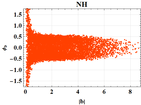
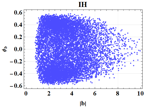
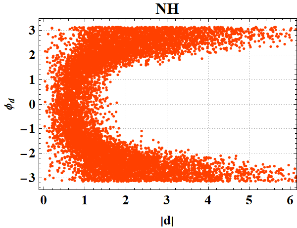
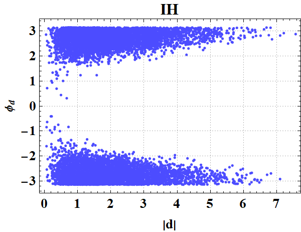
Figure 1: Case I - Correlation among the model parameters $\lvert b\rvert$, $\phi_{b}$ & $\lvert d\rvert$, $\phi_{d}$ in both NH (left column) as well as IH (right column).

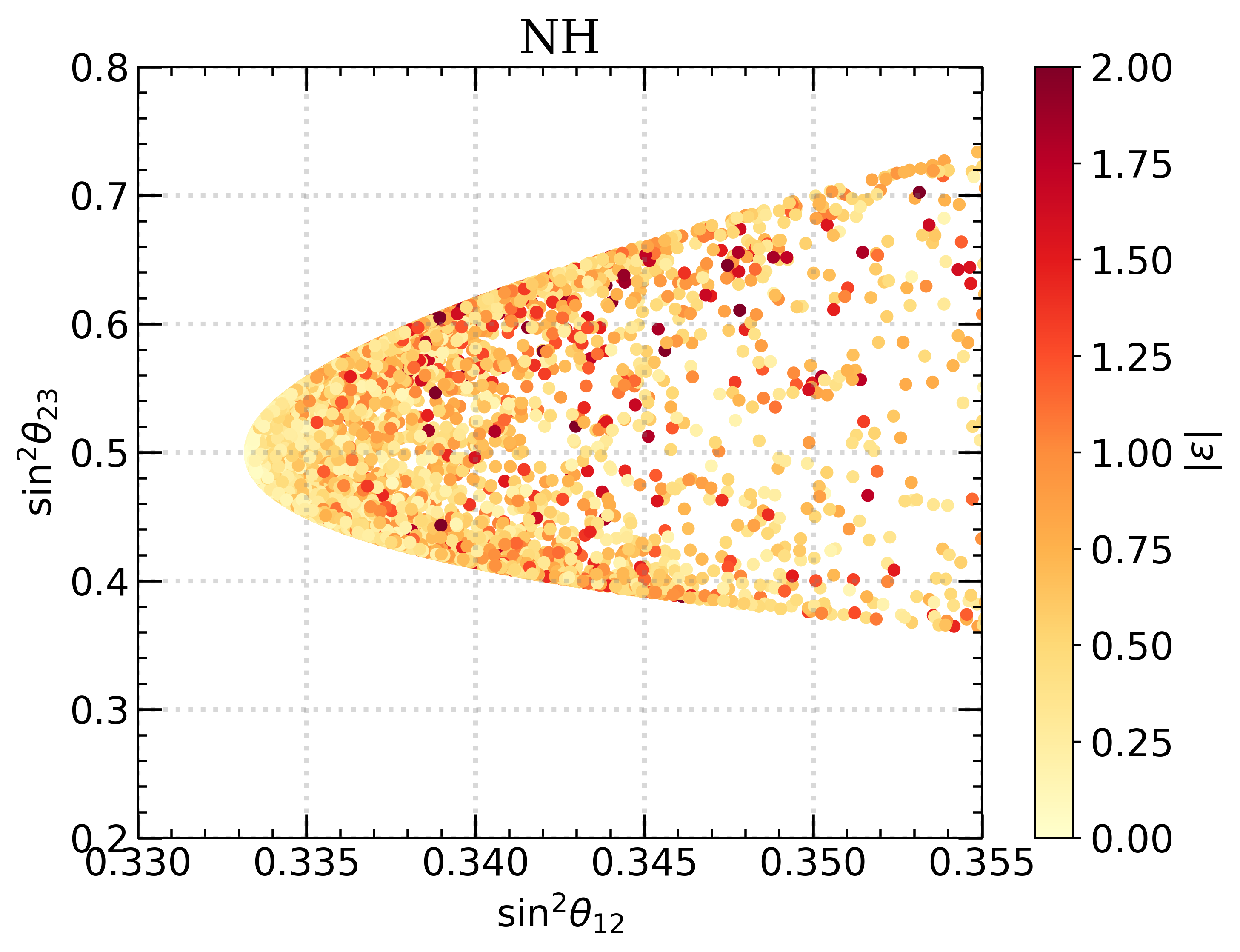
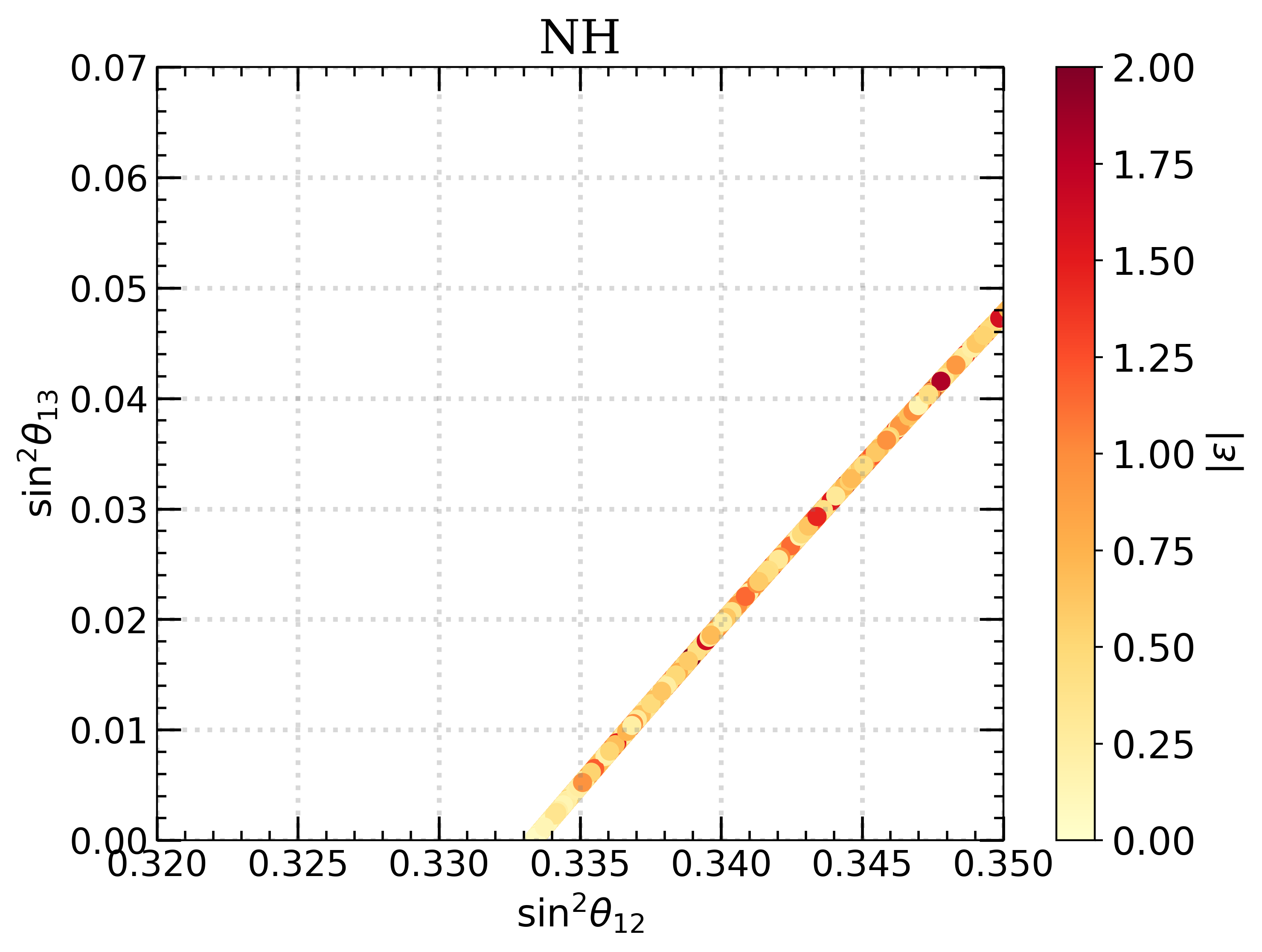
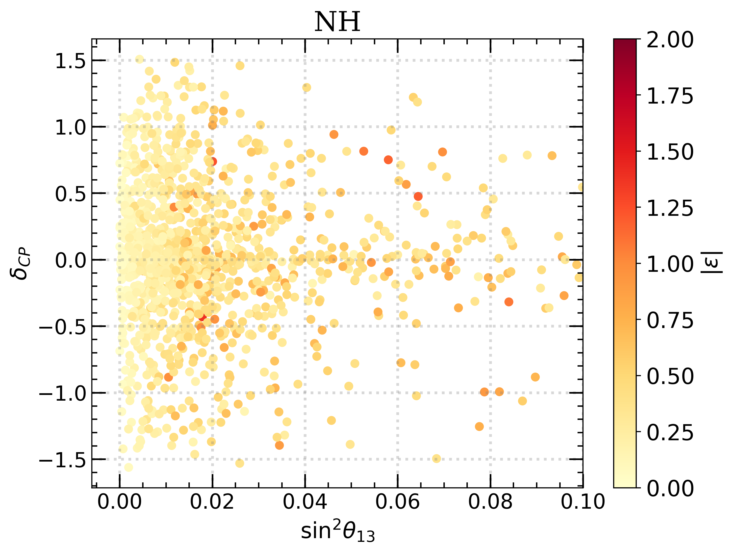
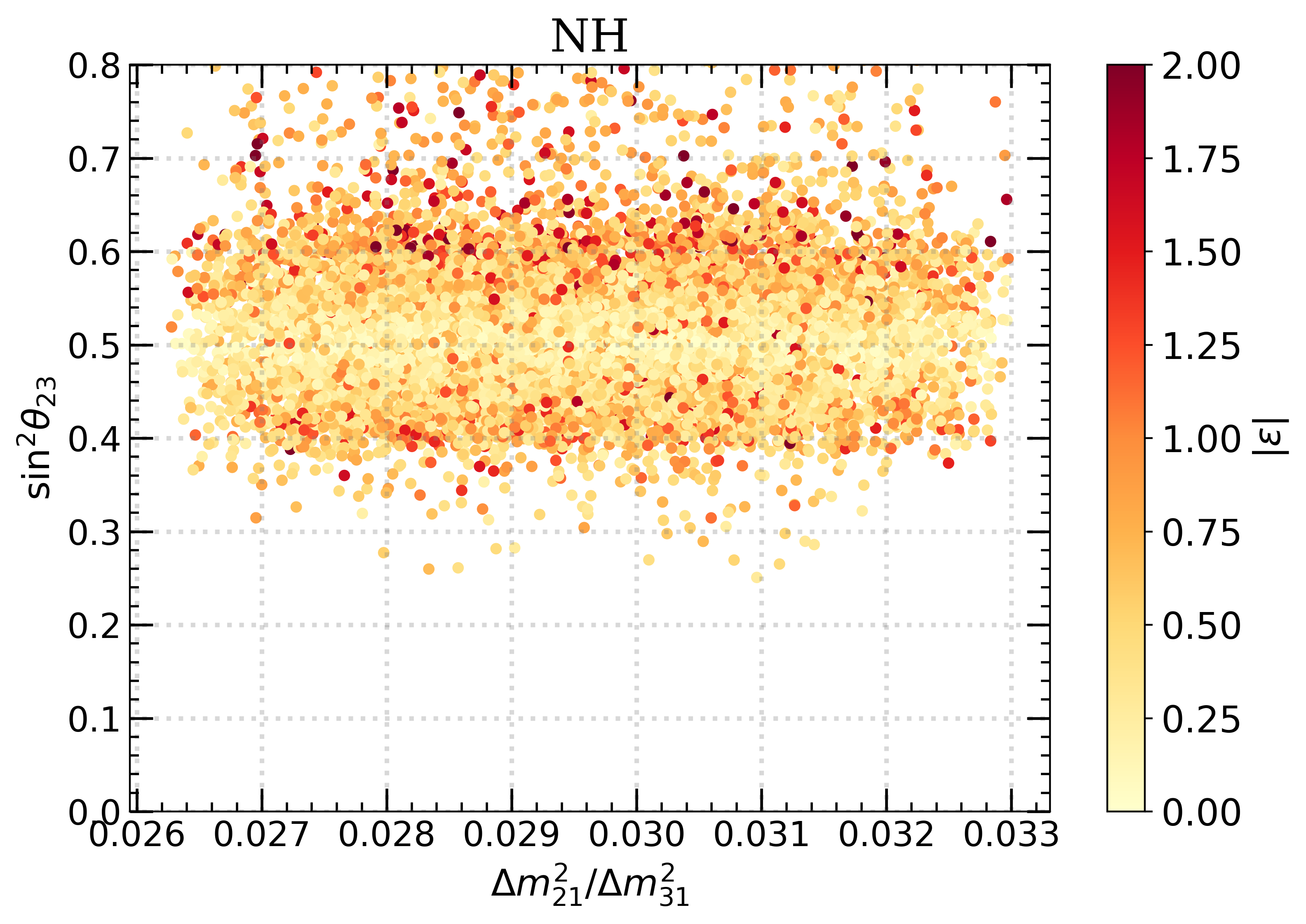
Figure 2: Case I - Variation of the mixing angles, mass-squared differences and Dirac CP phase with the correction parameter $\epsilon$ in NH case. The color-bar represents the different values of the correction parameter $\epsilon$.

First, we shall discuss case I, for perturbation parameter $\epsilon$. In Fig. 1, we have shown the parameter space of the model for Case I, which is constrained using the 3$\sigma$ bound on neutrino oscillation data (Table 1). For both normal and inverted hierarchies, one can see that there is a high correlation between different parameters of the model.

Fig. 2 shows the prediction of the various neutrino oscillation parameters for NH in case I. The calculated best fit values of $\sin^{2}\theta_{12}$, $\sin^{2}\theta_{13}$ and $\sin^{2}\theta_{23}$ are (0.341, 0.023, 0.62) which are within the 3$\sigma$ range of experimental values. Other parameters such as $\Delta m_{21}^{2}$, $\Delta m_{31}^{2}$ and $\delta_{CP}$ have their best-fit values, corresponding to $\chi^{2}$-minimum, at ($7.422\times 10^{-5}eV^{2}$, $2.556\times 10^{-3}eV^{2}$, $-0.367\pi$) respectively, which perfectly agreed with the latest observed neutrino oscillation experimental data. Similar variation of $\sin^{2}\theta_{13}$ and $\sin^{2}\theta_{23}$ with increase in $\lvert\epsilon\rvert$ is observed for IH.

Fig. 3 gives the neutrino oscillation parameters predicted by the model for IH. (0.341, 0.024, 0.61) are the best fit values of $\sin^{2}\theta_{12}$, $\sin^{2}\theta_{13}$ and $\sin^{2}\theta_{23}$, which are all within the 3 $\sigma$ range of experimental values. Also, $\Delta m_{21}^{2}$, $\Delta m_{31}^{2}$ and $\delta_{CP}$ have their best-fit values, corresponding to $\chi^{2}$-minimum, at ($7.465\times 10^{-5}eV^{2}$, $2.492\times 10^{-3}eV^{2}$, $0.39\pi$). Besides, we determined that, as the correction parameter $\lvert\epsilon\rvert$ increases, the value of $\sin^{2}\theta_{13}$ and $\sin^{2}\theta_{23}$ moves away from 0 and $\frac{1}{2}$, respectively.

Thus, the model defined in Case I, clearly shows that the deviation from exact tri-bimaximal mixing, however, with the change in $\lvert\epsilon\rvert$ there is no observable preference for the octant of $\theta_{23}$.

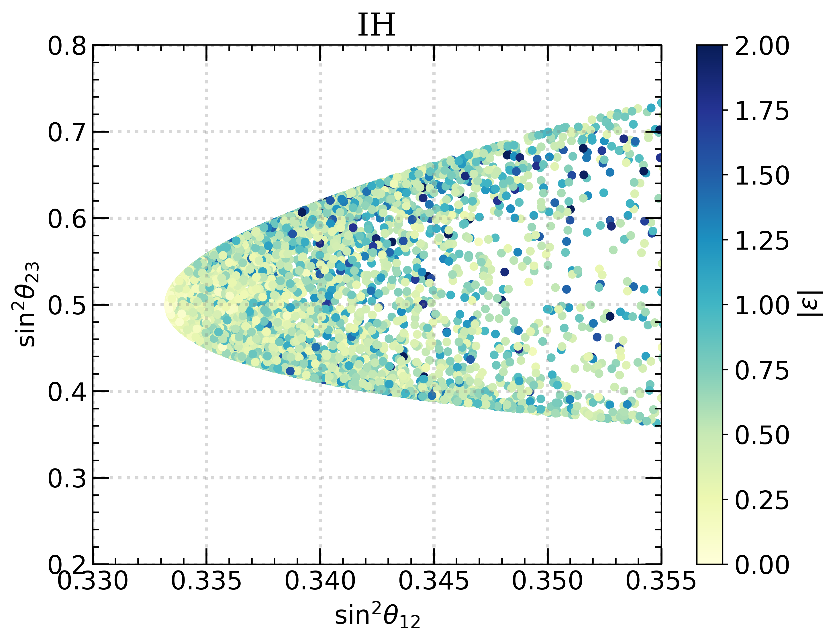
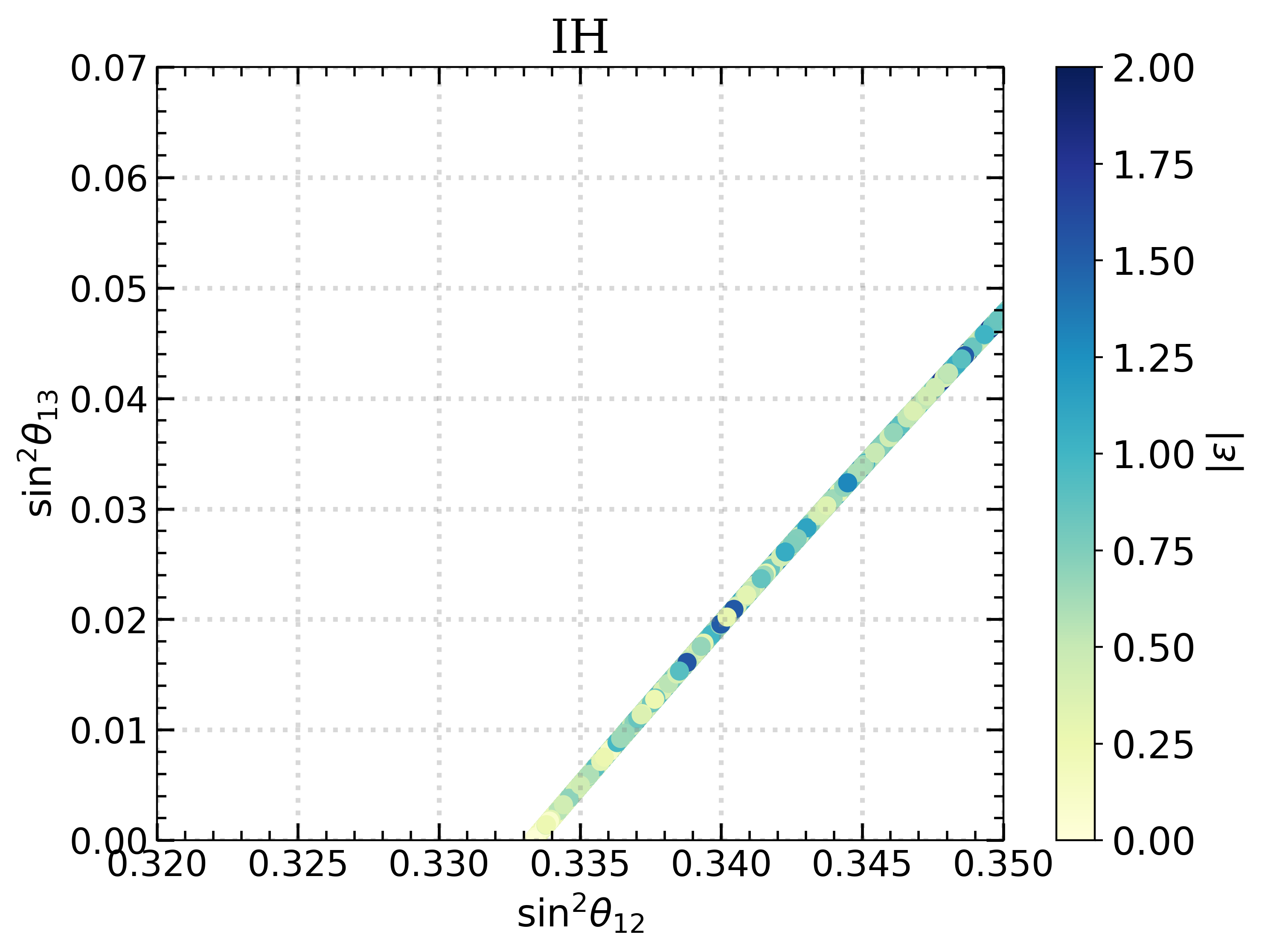
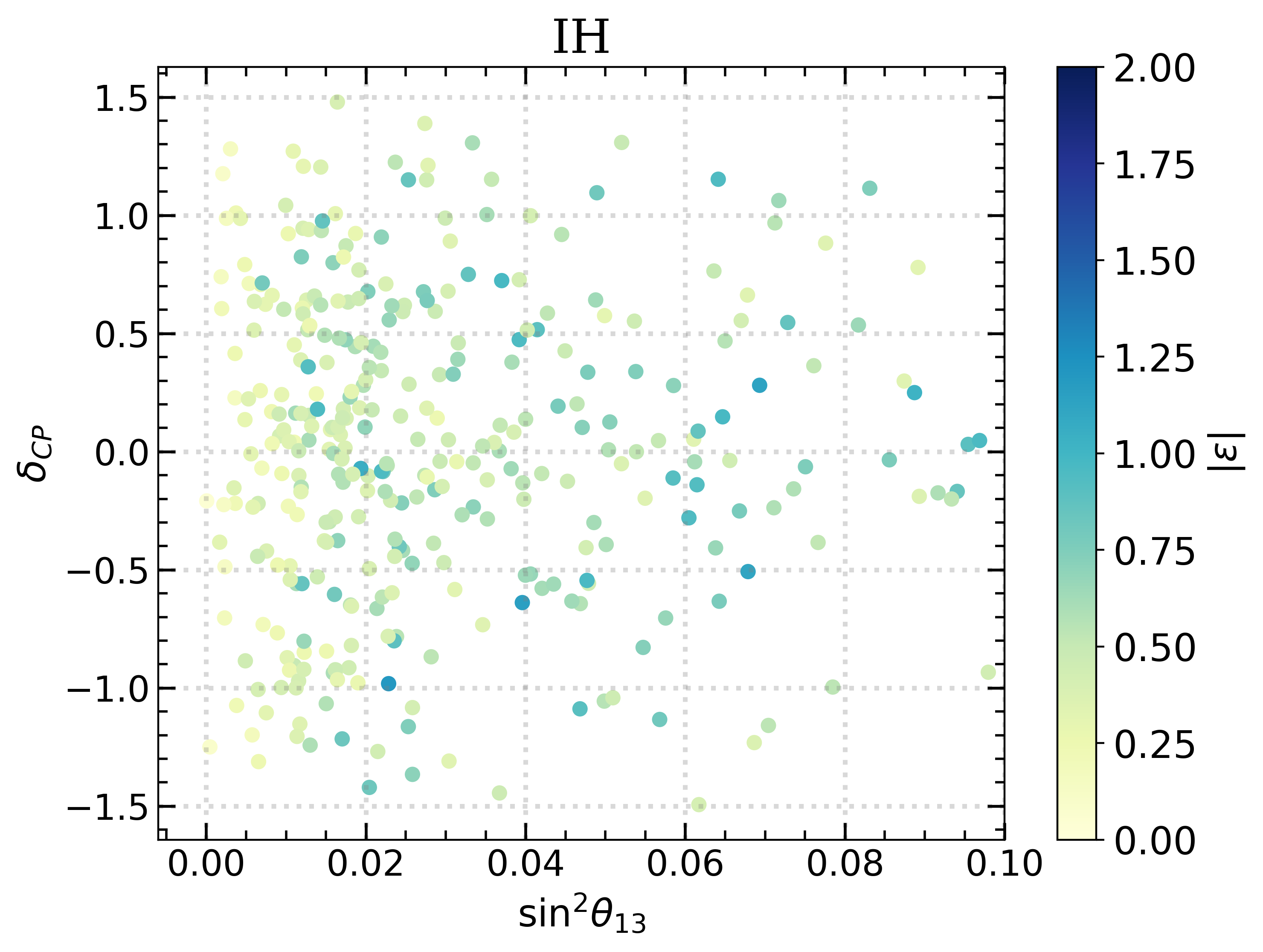
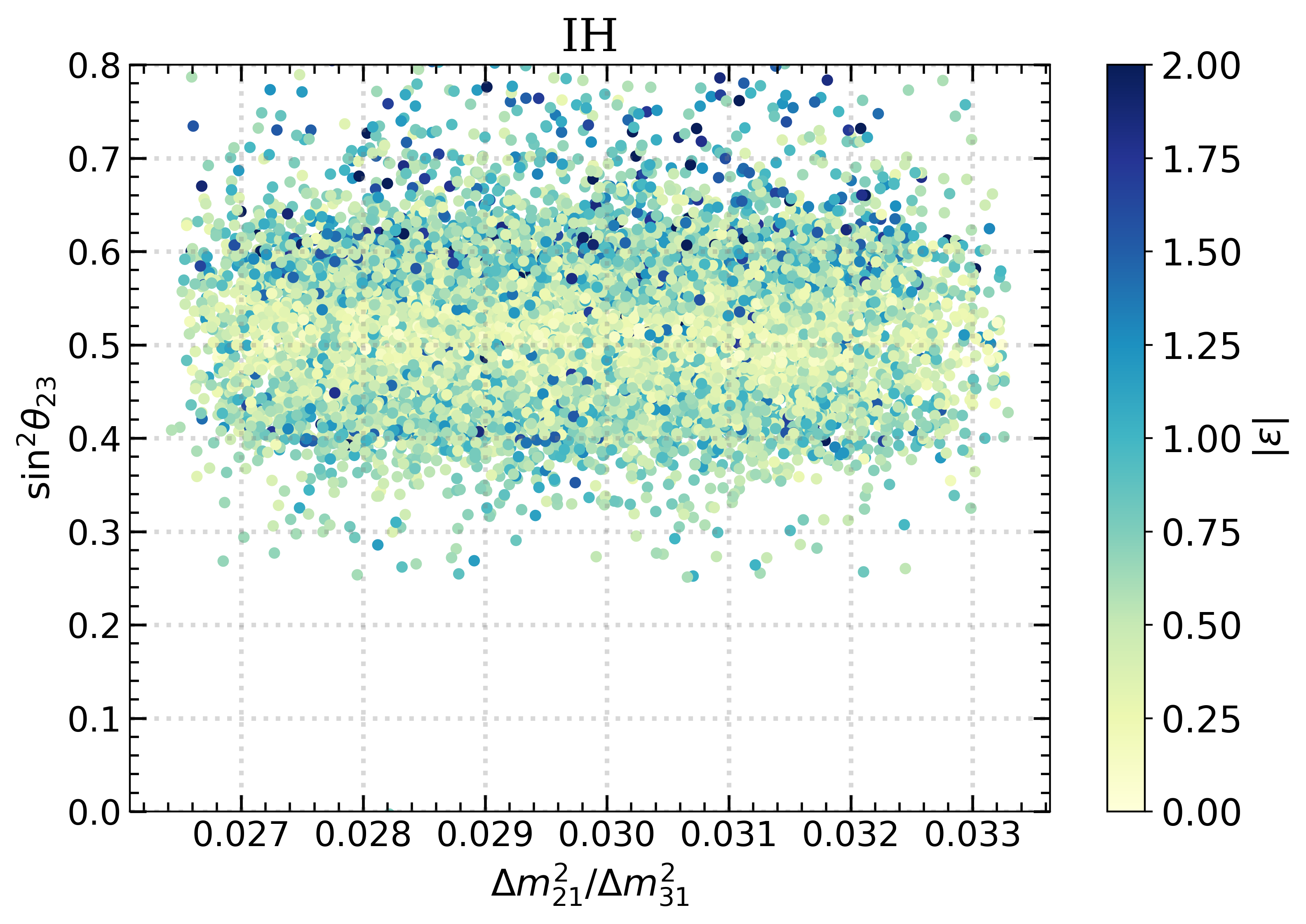
Figure 3: Case I - Variation of the mixing angles, mass-squared differences and Dirac CP phase with the correction parameter $\epsilon$ in IH case. The color-bar represents the different values of the correction parameter $\epsilon$.

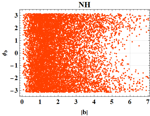
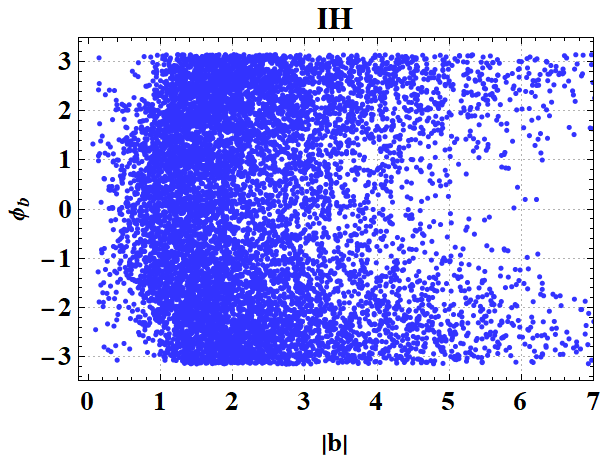
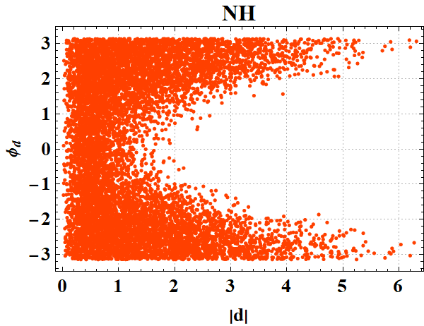
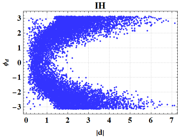
Figure 4: Case II - Correlation among the model parameters $\lvert b\rvert$, $\phi_{b}$ & $\lvert d\rvert$, $\phi_{d}$ in both NH (left column) as well as IH (right column).

Now, we discuss for the case II for the perturbation parameter $\epsilon^{\prime}$. In Figs. 4 and 5, we show the results with second type of correction, described as Case II in section II.2. The allowed ranges for the model parameters for both NH as well as IH are presented in Fig. 4. Also, the different correlation plots among the various neutrino oscillation parameters and their variations with $\lvert\epsilon^{\prime}\rvert$ are shown in fig. 5. It is clear that the neutrino mixing deviates from exact TBM mixing as $\lvert\epsilon^{\prime}\rvert$ increases from 0 in both NH and IH cases. The prediction of the atmospheric mixing angle $\theta_{23}$ in NH case shows slight preference towards lower octant for larger values of $\epsilon^{\prime}$. Thus, the modification of Altarelli-Feruglio with additional term, $x_{\epsilon}^{\prime}\xi^{\prime}{(ll)}^{\prime\prime}\frac{\rho\rho}{\Lambda^{2}}$, allows us to deviate from TBM mixing. The best-fit values for the predictions of the various oscillation parameters is shown in Table 3.

Parameter	NH	IH
$\sin^{2}\theta_{12}$	0.3407	0.341
$\sin^{2}\theta_{13}$	0.0217	0.0226
$\sin^{2}\theta_{23}$	0.576	0.547
$\delta_{CP}$	0.061 $\pi$	0.145 $\pi$
$\Delta m_{21}^{2}$	$7.498\times 10^{-5}$	$7.492\times 10^{-5}$
$\Delta m_{31}^{2}$	$2.517\times 10^{-3}$	$2.484\times 10^{-5}$

Table 3: Case II- Best-fit values for different parameters predicted by the model

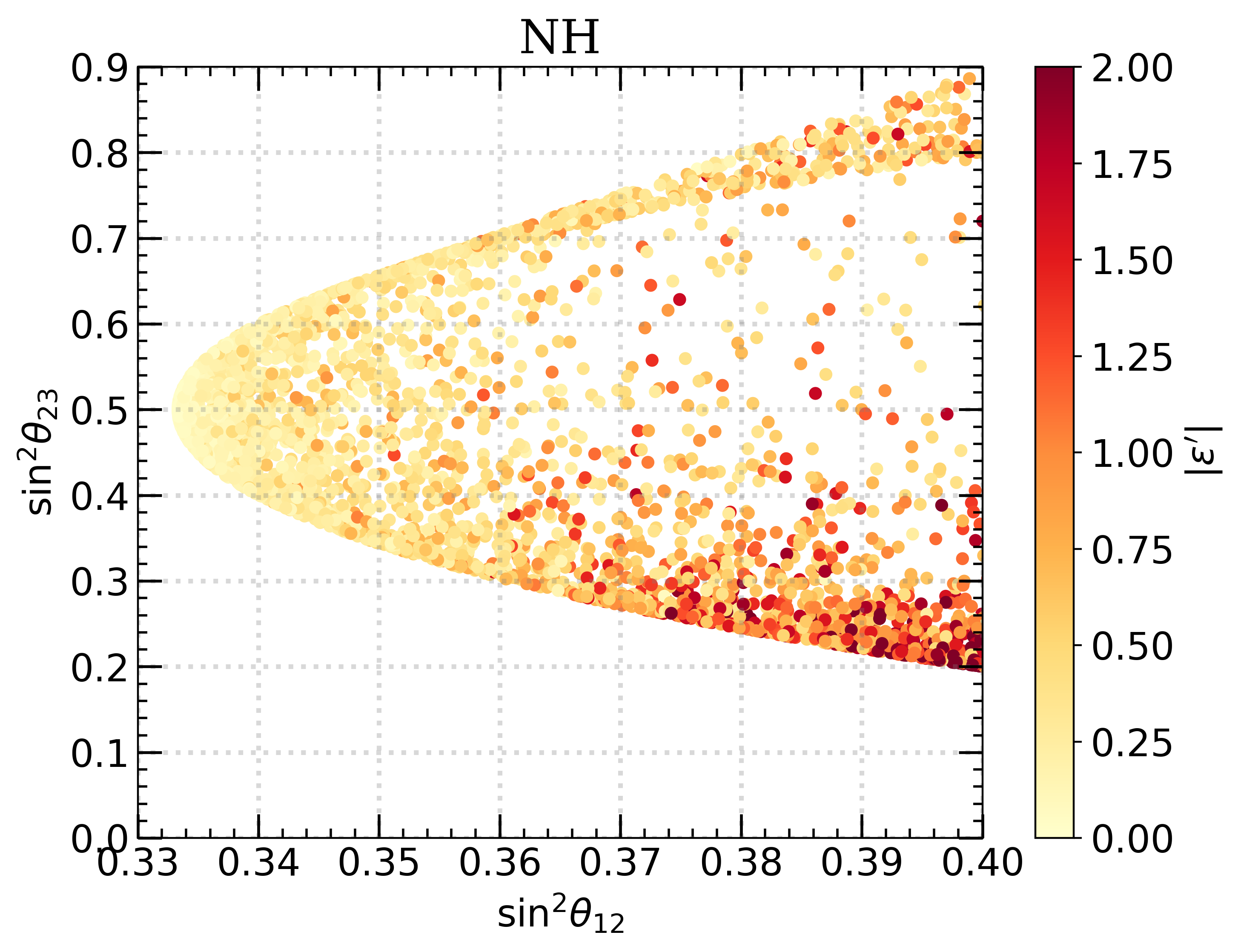
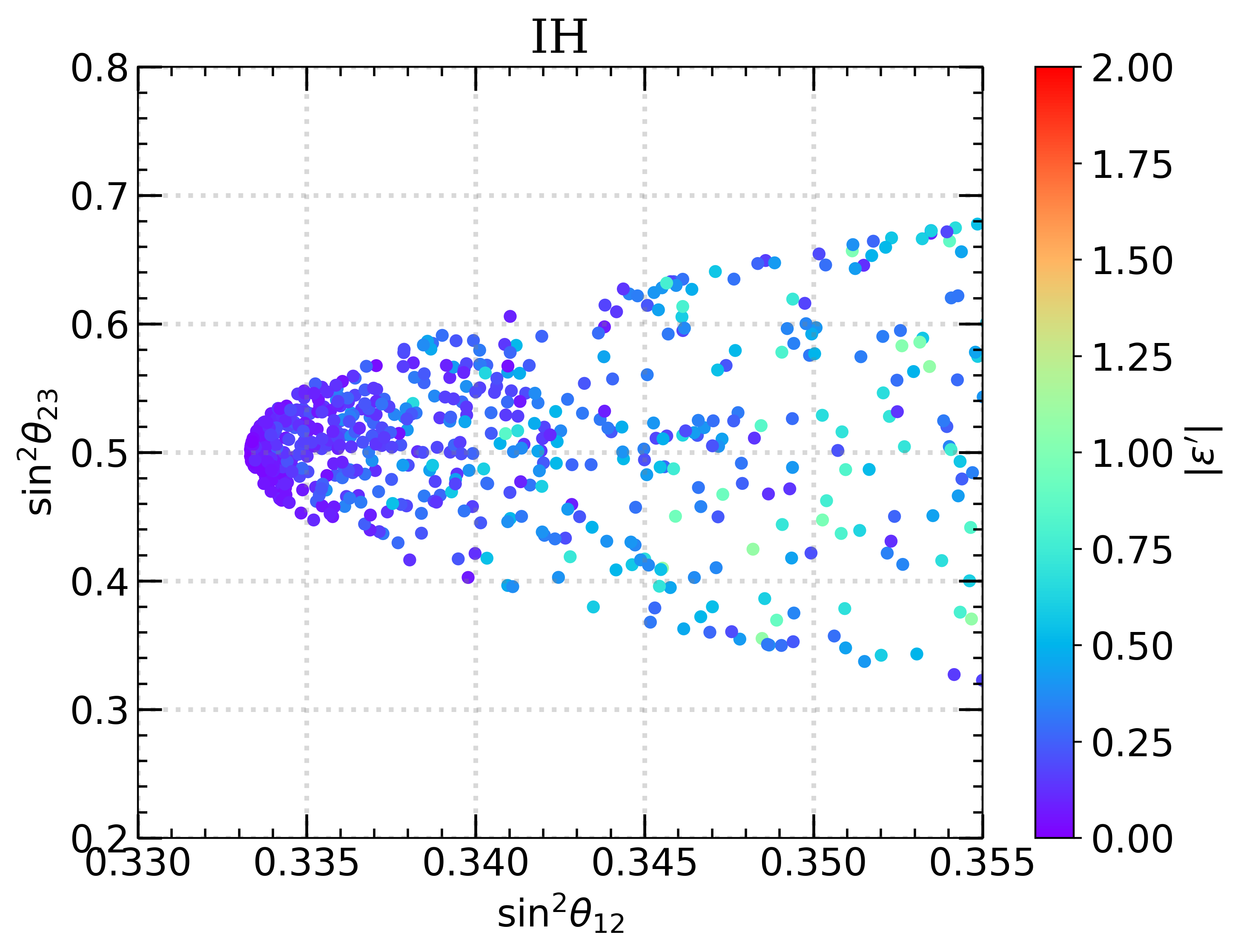
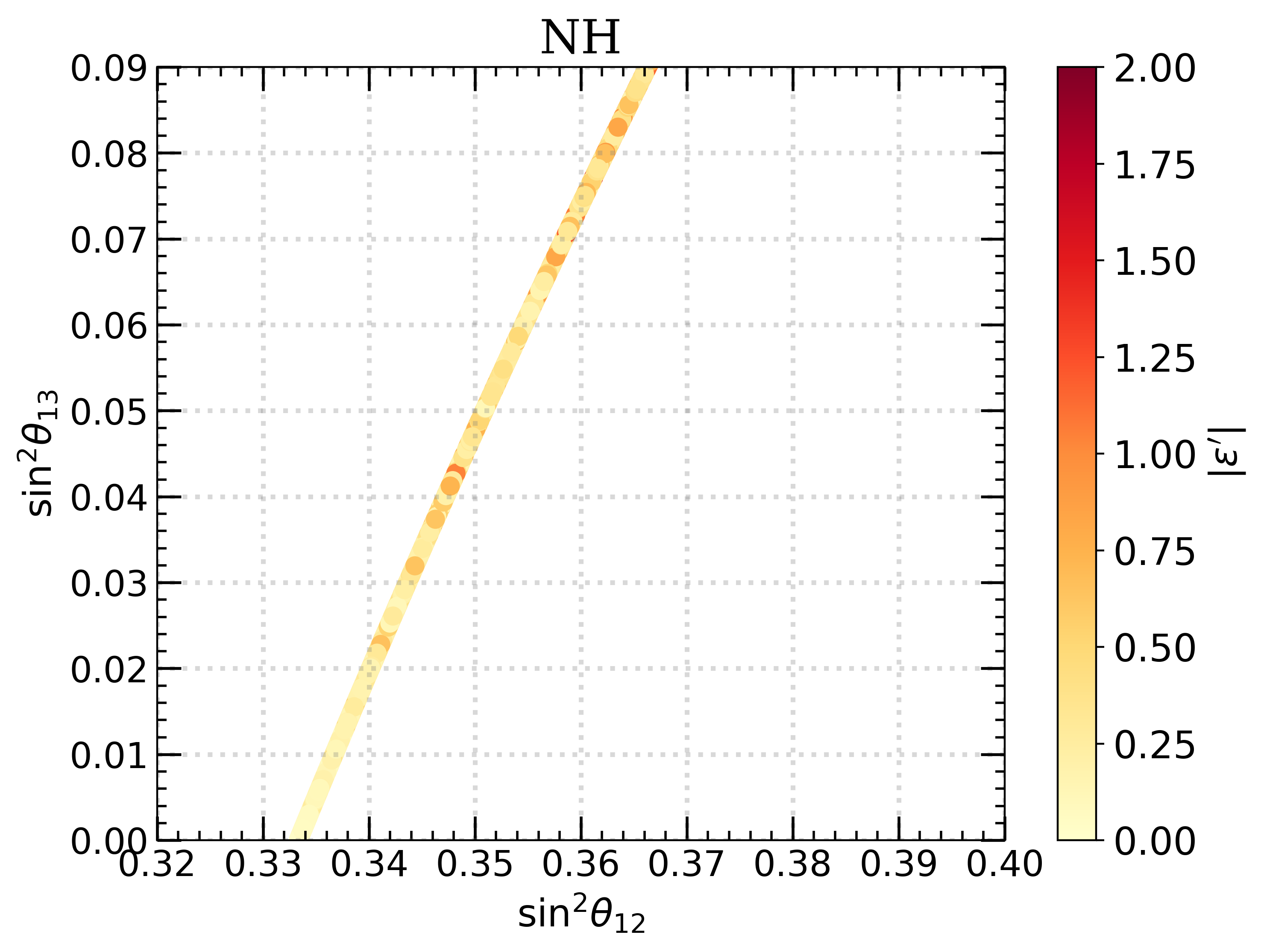
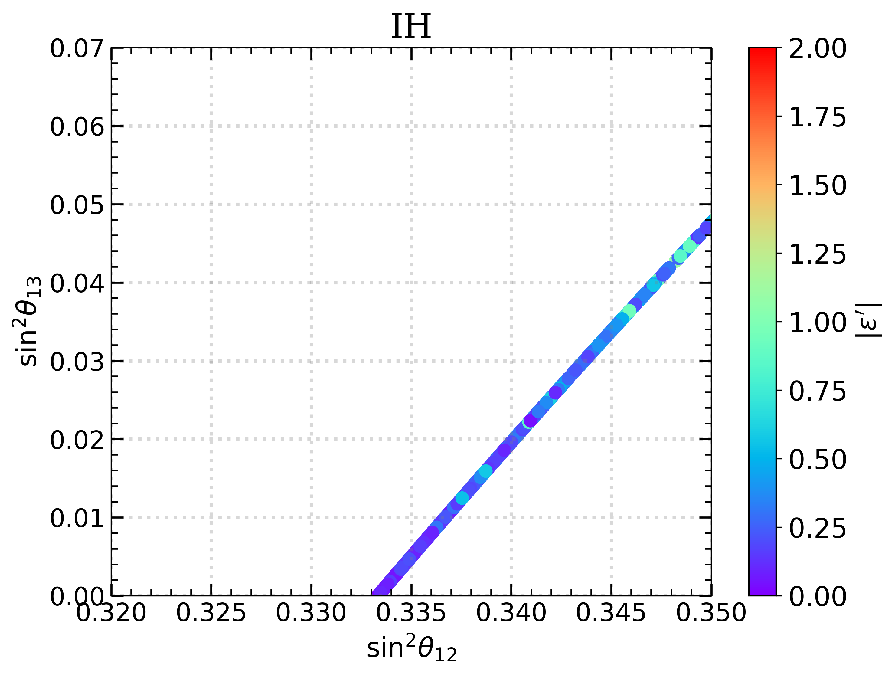
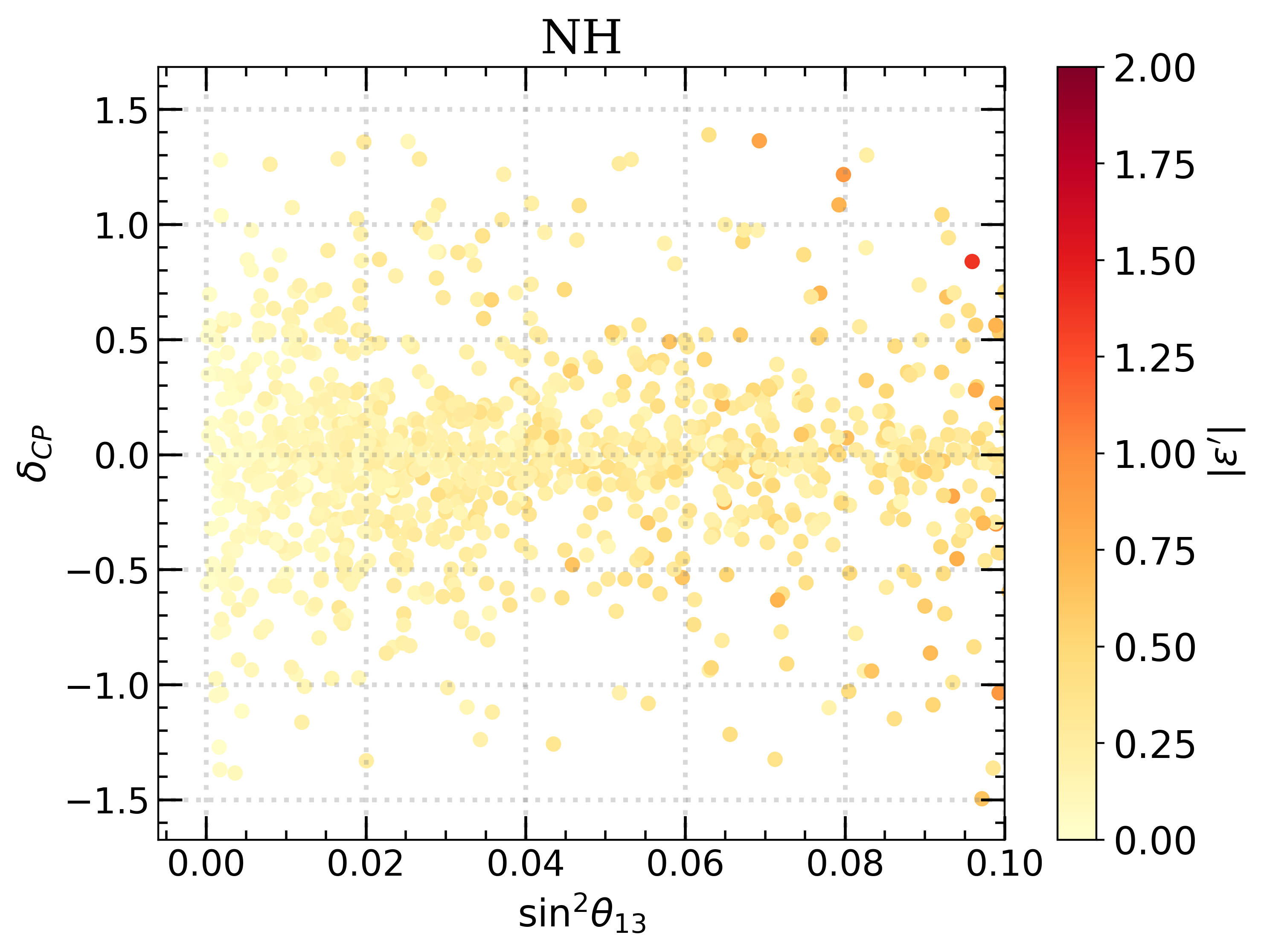
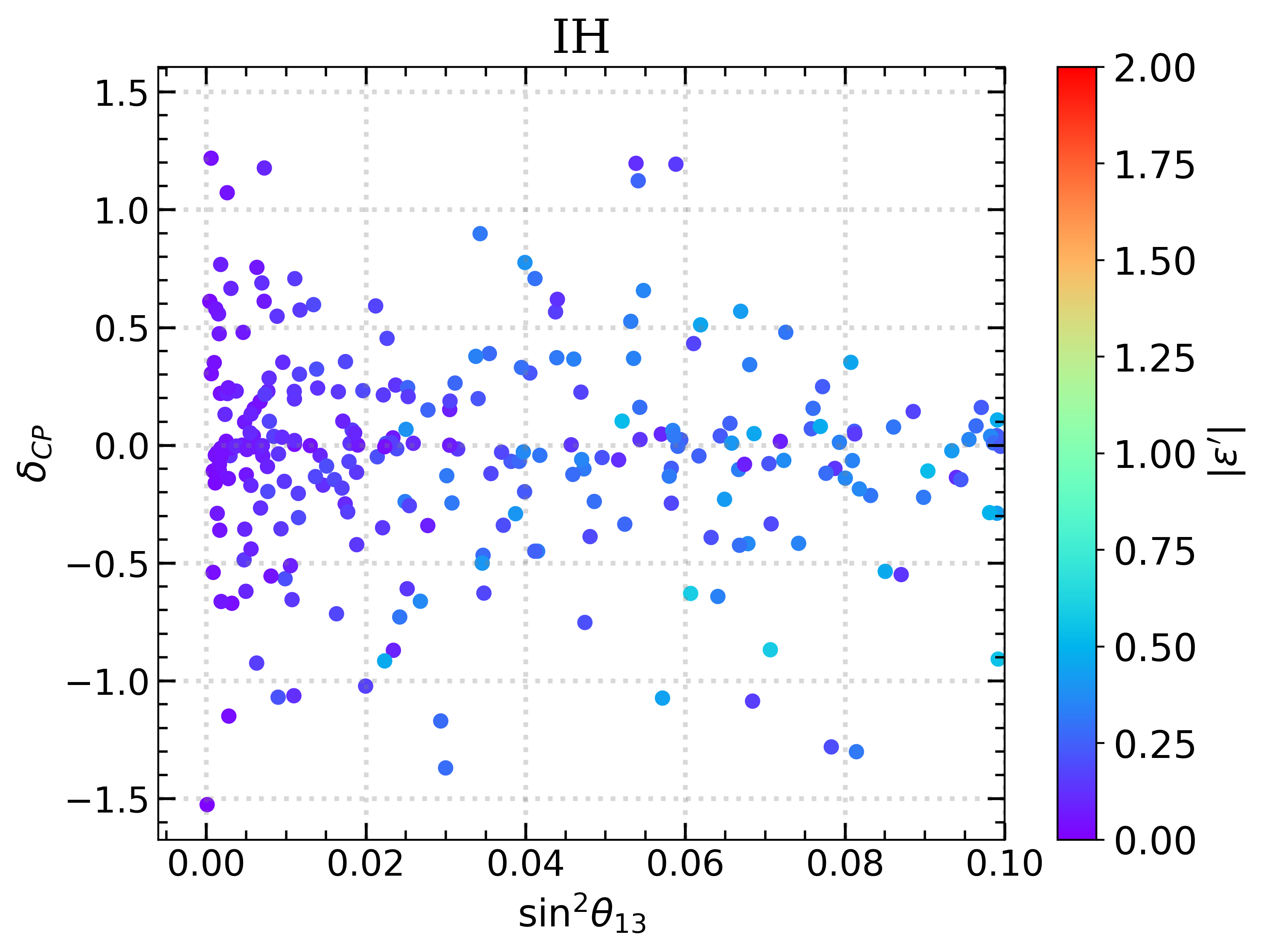
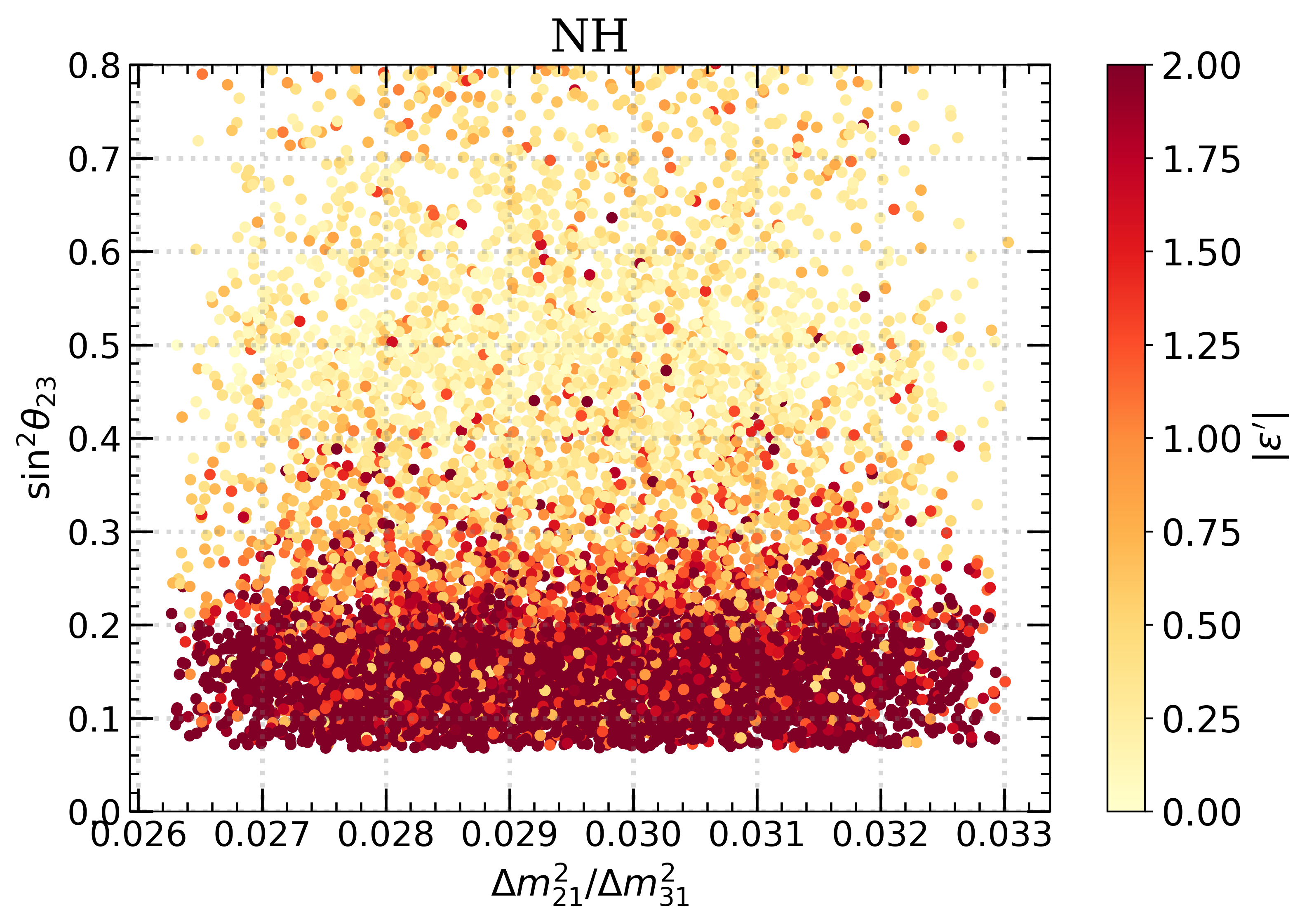
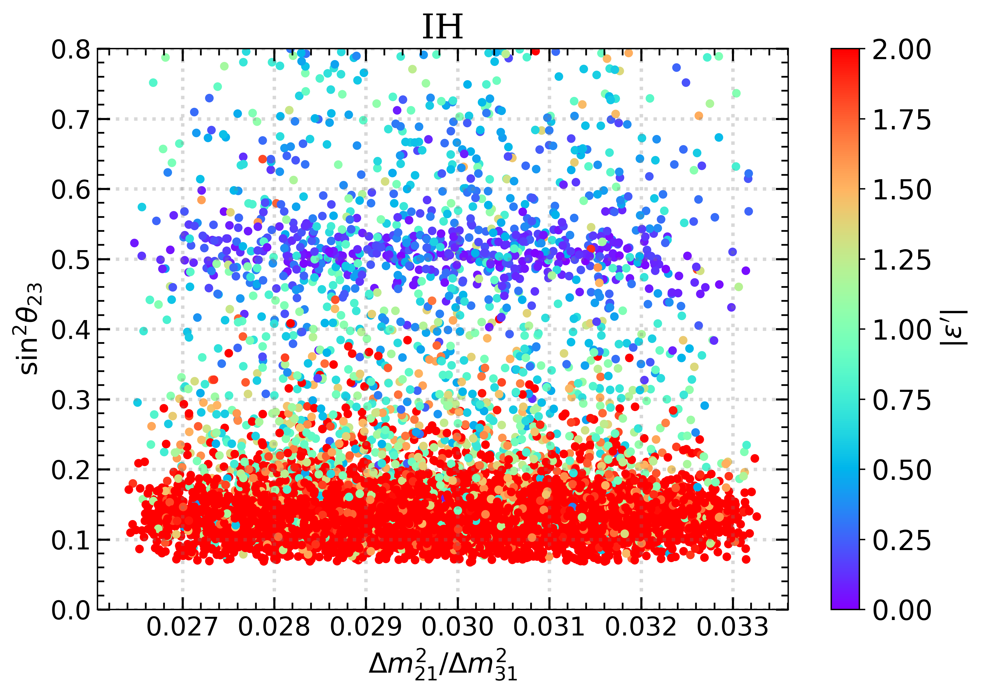
Figure 5: Case II - Variation of the mixing angles, mass-squared differences and Dirac CP phase with the correction parameter $\epsilon^{\prime}$ in NH (left) and IH(right) case. The color-bar represents the different values of the correction parameter $\epsilon^{\prime}$.

III.1 Neutrinoless double beta decay (NDBD):

Additionally, we are unsure about the nature of neutrinos - whether Majorana or Dirac. For neutrino to be Majorana in nature, the study of NDBD is very important. There are some ongoing NDBD experiments to determine Majorana nature of neutrino. The effective mass that governs the process is provided by,

$$m_{\beta\beta}=U^{2}_{Li}m_{i}$$ (17)

where $U_{Li}$ are the elements of the first row of the neutrino mixing matrix $U_{PMNS}$ (Eq.1) which is dependent on known parameters $\theta_{12}$, $\theta_{13}$ and the unknown Majorana phases $\alpha$ and $\beta$. $U_{PMNS}$ is the diagonalizing matrix of the light neutrino mass matrix $m_{\nu}$ so that,

$$m_{\nu}=U_{PMNS}M^{(diag)}_{\nu}U^{T}_{PMNS}$$ (18)

where, $M^{(diag)}_{\nu}$ =diag($m_{1}$, $m_{2}$, $m_{3}$). The effective Majorana mass can be parameterized using the diagonalizing matrix elements and the mass eigen values as follows:

$$m_{\beta\beta}=m_{1}c_{12}^{2}c^{2}_{13}+m_{2}s^{2}_{12}c^{2}_{13}e^{2i\alpha}+m_{3}s^{2}_{13}e^{2i\beta}$$ (19)

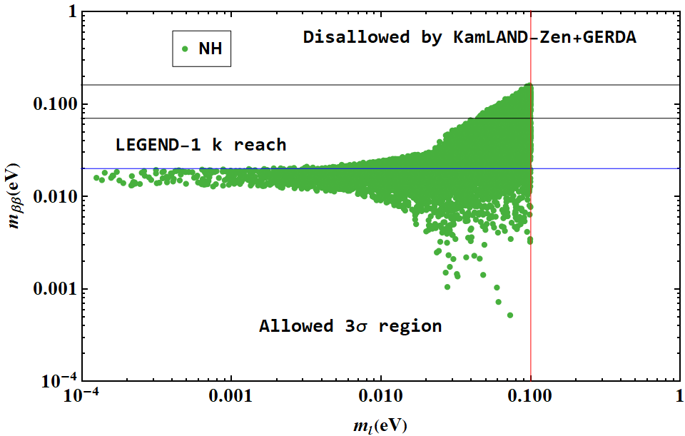
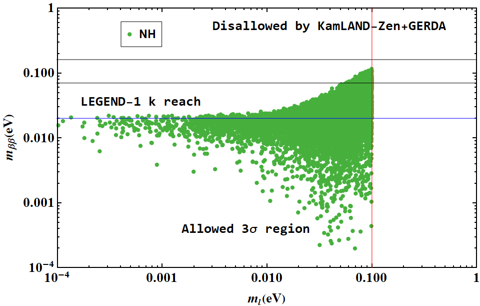
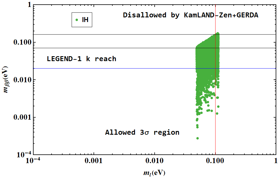
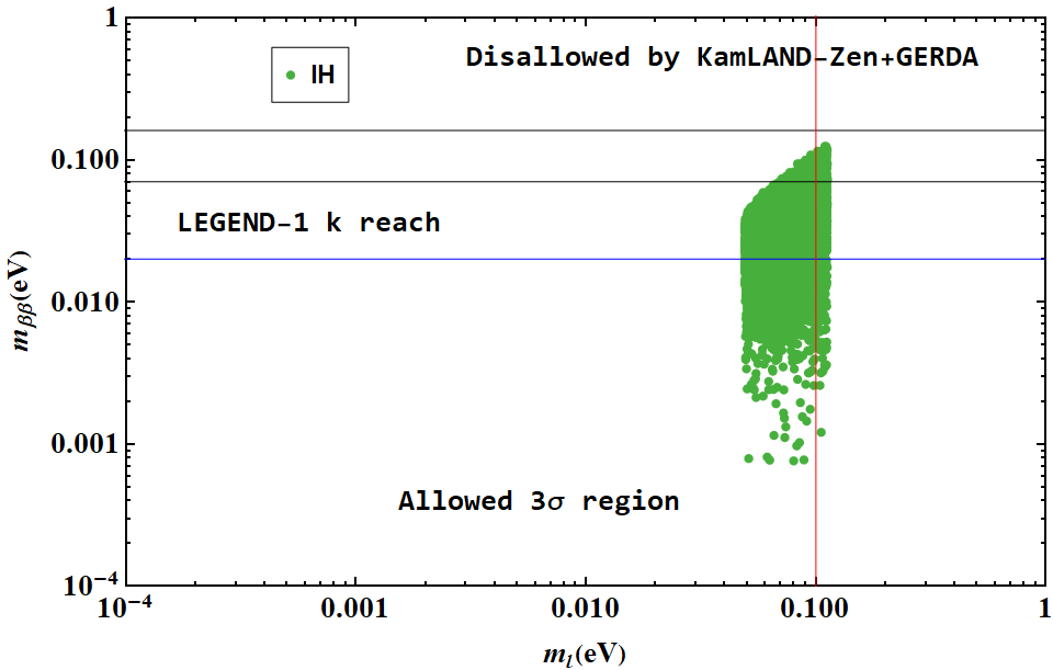
Figure 6: Variation of effective Majorana neutrino mass with lighest neutrino mass in case I (left panel) and case II (right panel). The red solid line represents the cosmological bound on the sum of the absolute neutrino mass. The black solid line represents the KamLAND-Zen bound on the effective mass.

Using the constrained parameter space, we have evaluated the value of $m_{\beta\beta}$ for case I and case II in both NH as well as IH cases. The variation of $m_{\beta\beta}$ with lightest neutrino mass is shown in Figure 6 for both the neutrino mass hierarchies. The sensitivity reach of NDBD experiments like KamLAND-Zen Gando (2020); Biller (2021), GERDA Di Marco (2020); Agostini et al. (2020); D’Andrea (2020), LEGEND-1k Abgrall et al. (2021) is also shown in figure 6. $m_{\beta\beta}$ is found to be well within the sensitivity reach of these NDBD experiments for both the cases, (I) and (II).

IV Conclusion

We have constructed a flavon-symmetric $A_{4}\times Z_{2}\times Z_{3}$ model to realize the latest neutrino oscillation experimental data which depart from Tribimaximal neutrino mixing pattern. The models have been checked for accuracy by adding three extra flavons $\xi^{\prime}$, $\xi^{\prime\prime}$, and $\rho$ transforming under representations of $A_{4}$ to extend the A-F model. And the cyclic $Z_{2}\times Z_{3}$ symmetric term has been incorporated to eliminate unwanted terms in the calculations. The calculated two perturbation parameters $\epsilon$ and $\epsilon^{\prime}$ clearly showed the deviation of neutrino mixing parameters from exact Tri-bimaximal neutrino mixing matrix. The resulting mass matrices give predictions for the neutrino oscillation parameters and their best-fit values are obtained using the $\chi^{2}$-analysis, which are consistent with the latest global neutrino oscillation experimental data. We found the magnitude of deviations from TBM is dominated by VEV of $\rho$. However, these quantities and corrections have little discriminative power, hence we supplement with observables related to neutrino mass. Therefore, we have also investigated NDBD in our model. The scatter plots of NDBD parameter ($m_{\beta\beta}$) and the lightest neutrino mass ($m_{l}$) parameter space are different in each model and allowed us to distinguish different models. The value of effective Majorana neutrino mass $|m_{\beta\beta}|$ is well within the sensitivity reach of the recent NDBD experiments like KamLAND- Zen, GERDA and LEGEND-1k. The determination of NDBD, cosmological mass and leptonic CP-violation phase $\delta_{CP}$ which are consistent with the latest experimental data will discriminate the neutrino mass models.

Appendix A

Field	$l$	$e^{c}$	$\mu^{c}$	$\tau^{c}$	$h_{u}$	$h_{d}$	$\Phi_{S}$	$\Phi_{T}$	$\xi$	$\xi^{\prime}$	$\xi^{\prime\prime}$	$\rho$	$\phi^{T}_{0}$	$\phi^{S}_{0}$	$\xi_{0}$
SU(2)	2	1	1	1	2	2	1	1	1	1	1	1	-	-	-
A4	3	1	$1^{\prime\prime}$	$1^{\prime}$	1	1	3	3	1	$1^{\prime}$	$1^{\prime\prime}$	1	3	3	1
Z3	$\omega$	$\omega^{2}$	$\omega^{2}$	$\omega^{2}$	1	1	$\omega$	1	$\omega$	$\omega$	$\omega$	1	1	$\omega$	$\omega$
Z2	l	1	1	1	1	1	1	1	1	1	1	-1	1	1	1

Table 4: Full particle content of our model with associated “driving fields” $\phi^{T}_{0}$, $\phi^{S}_{0}$ and $\xi_{0}$.

The superpotential of the model with the “driving fields” $\phi^{T}_{0}$, $\phi^{S}_{0}$ and $\xi_{0}$ that allows to build the scalar potentials in the symmetry breaking sector, reads as

$$W= M(\phi^{T}_{0}\phi_{T})+g(\phi^{T}_{0}\phi_{T}\phi_{T})+g_{1}(\phi^{S}_{0}\phi_{S}\phi_{S})+g_{2}\xi(\phi^{S}_{0}\phi_{S})+g_{3}\xi^{\prime}(\xi^{S}_{0}\xi_{S})$$

$$+g_{4}\xi^{\prime\prime}(\xi^{S}_{0}\xi_{S})+g_{5}\xi_{0}(\phi_{S}\phi_{S})+g_{6}\xi_{0}\xi^{2}+g_{7}\xi_{0}\xi^{\prime}\xi^{\prime\prime}$$ (20)

At this level there is no fundamental distinction among the singlets $\xi$, $\xi^{\prime}$ and $\xi^{\prime\prime}$. So, we can consider $\phi^{S}_{0}\phi_{S}$ is coupling with $\xi$ only.

We use,

$$\phi_{T}=[\phi^{1}_{T},\phi^{2}_{T},\phi^{3}_{T}],\quad\phi^{T}_{0}=[\phi^{T}_{01},\phi^{T}_{02},\phi^{T}_{03}]$$

$$\phi_{S}=[\phi^{1}_{S},\phi^{2}_{S},\phi^{3}_{S}],\quad\phi^{S}_{0}=[\phi^{S}_{01},\phi^{S}_{02},\phi^{S}_{03}]$$

Now,

$$\frac{\delta W}{\delta\phi^{T}_{01}} =M\phi^{1}_{T}+g.\frac{1}{3}.[{2\phi^{1}_{T}\phi^{1}_{T}-\phi^{2}_{T}\phi^{3}_{T}-\phi^{3}_{T}\phi^{2}_{T}}]=0$$ (21)

$$\frac{\delta W}{\delta\phi^{T}_{02}} =M\phi^{3}_{T}+g.\frac{1}{3}.[{2\phi^{3}_{T}\phi^{3}_{T}-\phi^{1}_{T}\phi^{2}_{T}-\phi^{2}_{T}\phi^{1}_{T}}]=0$$ (22)

$$\frac{\delta W}{\delta\phi^{T}_{03}} =M\phi^{2}_{T}+g.\frac{1}{3}.[{2\phi^{2}_{T}\phi^{2}_{T}-\phi^{1}_{T}\phi^{3}_{T}-\phi^{3}_{T}\phi^{1}_{T}}]=0$$ (23)

$$\frac{\delta W}{\delta\phi^{S}_{01}} =g_{1}.\frac{1}{3}[2\phi^{1}_{S}\phi^{1}_{S}-\phi^{2}_{S}\phi^{3}_{S}-\phi^{3}_{S}\phi^{2}_{S}]+g_{2}\xi\phi^{1}_{S}=0$$ (24)

$$\frac{\delta W}{\delta\phi^{S}_{02}} =g_{1}.\frac{1}{3}[2\phi^{2}_{S}\phi^{2}_{S}-\phi^{1}_{S}\phi^{3}_{S}-\phi^{3}_{S}\phi^{1}_{S}]+g_{2}\xi\phi^{3}_{S}=0$$ (25)

$$\frac{\delta W}{\delta\phi^{S}_{03}} =g_{1}.\frac{1}{3}[2\phi^{3}_{S}\phi^{3}_{S}-\phi^{1}_{S}\phi^{2}_{S}-\phi^{2}_{S}\phi^{1}_{S}]+g_{2}\xi\phi^{2}_{S}=0$$ (26)

$$\frac{\delta W}{\delta\xi_{0}} =g_{5}.[\phi^{1}_{S}\phi^{1}_{S}+\phi^{2}_{S}\phi^{3}_{S}+\phi^{3}_{S}\phi^{2}_{S}]+g_{6}\xi^{2}+g_{7}\xi^{\prime}\xi^{\prime\prime}=0$$ (27)

A solution of the first three equation is:

$$\phi_{T}=(v_{T},0,0),v_{T}=-\frac{3M}{2g}$$

When we enforce $<\xi>=0$, in a finite portion of the parameter space, we find the solution as:

$$<\xi>=0,\quad<\xi^{\prime}>=u^{\prime},\quad<\xi^{\prime\prime}>=u^{\prime\prime}$$

$$\phi_{S} =(v_{S},v_{S},v_{S})$$

$$v^{2}_{S} =-\frac{g_{7}u^{\prime}u^{\prime\prime}}{3g_{5}}$$

References

- King et al. (2014) S. F. King, A. Merle, S. Morisi, Y. Shimizu, and M. Tanimoto, New J. Phys. 16, 045018 (2014), eprint 1402.4271.
- King (2004) S. F. King, Rept. Prog. Phys. 67, 107 (2004), eprint hep-ph/0310204.
- Cao et al. (2021) S. Cao, A. Nath, T. V. Ngoc, P. T. Quyen, N. T. Hong Van, and N. K. Francis, Phys. Rev. D 103, 112010 (2021), eprint 2009.08585.
- McDonald (2016) A. B. McDonald, Rev. Mod. Phys. 88, 030502 (2016).
- Kajita (2016) T. Kajita, Rev. Mod. Phys. 88, 030501 (2016).
- Vien (2020) V. V. Vien, Mod. Phys. Lett. A 35, 2050311 (2020).
- de Salas et al. (2021) P. F. de Salas, D. V. Forero, S. Gariazzo, P. Martínez-Miravé, O. Mena, C. A. Ternes, M. Tórtola, and J. W. F. Valle, JHEP 02, 071 (2021), eprint 2006.11237.
- King (2017) S. F. King, Prog. Part. Nucl. Phys. 94, 217 (2017), eprint 1701.04413.
- Phong Nguyen et al. (2020) T. Phong Nguyen, L. T. Hue, D. T. Si, and T. T. Thuc, PTEP 2020, 033B04 (2020), eprint 1711.05588.
- Nguyen et al. (2022) T. P. Nguyen, T. T. Thuc, D. T. Si, T. T. Hong, and L. T. Hue, PTEP 2022, 023B01 (2022), eprint 2011.12181.
- An et al. (2012) F. P. An et al. (Daya Bay), Phys. Rev. Lett. 108, 171803 (2012), eprint 1203.1669.
- Ahn et al. (2012) J. K. Ahn et al. (RENO), Phys. Rev. Lett. 108, 191802 (2012), eprint 1204.0626.
- Adamson et al. (2011) P. Adamson et al. (MINOS), Phys. Rev. Lett. 107, 181802 (2011), eprint 1108.0015.
- Abe et al. (2012) Y. Abe et al. (Double Chooz), Phys. Rev. Lett. 108, 131801 (2012), eprint 1112.6353.
- Abe et al. (2011) K. Abe et al. (T2K), Phys. Rev. Lett. 107, 041801 (2011), eprint 1106.2822.
- Furry (1939) W. H. Furry, Phys. Rev. 56, 1184 (1939).
- Dell’Oro et al. (2016) S. Dell’Oro, S. Marcocci, M. Viel, and F. Vissani, Adv. High Energy Phys. 2016, 2162659 (2016), eprint 1601.07512.
- Bilenky and Giunti (2012) S. M. Bilenky and C. Giunti, Mod. Phys. Lett. A 27, 1230015 (2012), eprint 1203.5250.
- Weinberg (1979) S. Weinberg, Phys. Rev. Lett. 43, 1566 (1979).
- Yanagida (1980) T. Yanagida, Prog. Theor. Phys. 64, 1103 (1980).
- Minkowski (1977) P. Minkowski, Phys. Lett. B 67, 421 (1977).
- Das and Das (2020) P. Das and M. K. Das, Int. J. Mod. Phys. A 35, 2050125 (2020), eprint 1908.08417.
- Gell-Mann (1979) M. Gell-Mann, Supergravity, P. van Nieuwenhuizen and DZ Freedman eds., North Holland, Amsterdam The Netherlands 315 (1979).
- Mohapatra and Senjanovic (1980) R. N. Mohapatra and G. Senjanovic, Phys. Rev. Lett. 44, 912 (1980).
- Fukuyama and Nishiura (1997) T. Fukuyama and H. Nishiura (1997), eprint hep-ph/9702253.
- Vien et al. (2019) V. V. Vien, H. N. Long, and A. E. Cárcamo Hernández, PTEP 2019, 113B04 (2019), eprint 1909.09532.
- Yanagida (1979) T. Yanagida, in Workshop on unified theory and baryon number in the universe (KEK, Tsukuba, Japan, 1979).
- Boruah and Das (2022) B. B. Boruah and M. K. Das, Int. J. Mod. Phys. A 37, 2250026 (2022), eprint 2111.10341.
- Ma (1998) E. Ma, PoS corfu98, 047 (1998), eprint hep-ph/9902450.
- Csaki (1996) C. Csaki, Mod. Phys. Lett. A 11, 599 (1996), eprint hep-ph/9606414.
- Ellwanger et al. (2010) U. Ellwanger, C. Hugonie, and A. M. Teixeira, Phys. Rept. 496, 1 (2010), eprint 0910.1785.
- Ibanez and Uranga (2012) L. E. Ibanez and A. M. Uranga, String theory and particle physics: An introduction to string phenomenology (Cambridge University Press, 2012), ISBN 978-0-521-51752-2, 978-1-139-22742-1.
- Arkani-Hamed et al. (2001) N. Arkani-Hamed, S. Dimopoulos, G. R. Dvali, and J. March-Russell, Phys. Rev. D 65, 024032 (2001), eprint hep-ph/9811448.
- Ma (2006a) E. Ma, Phys. Rev. D 73, 077301 (2006a), eprint hep-ph/0601225.
- Aker et al. (2019) M. Aker, K. Altenmüller, M. Arenz, M. Babutzka, J. Barrett, S. Bauer, M. Beck, A. Beglarian, J. Behrens, T. Bergmann, et al., Physical review letters 123, 221802 (2019).
- Francis (2014) N. K. Francis, Adv. High Energy Phys. 2014, 689719 (2014).
- Group et al. (2020) P. D. Group, P. Zyla, R. Barnett, J. Beringer, O. Dahl, D. Dwyer, D. Groom, C.-J. Lin, K. Lugovsky, E. Pianori, et al., Progress of Theoretical and Experimental Physics 2020, 083C01 (2020).
- Nath and Francis (2021) A. Nath and N. K. Francis, Int. J. Mod. Phys. A 36, 2130008 (2021), eprint 1804.08467.
- Harrison et al. (2002) P. F. Harrison, D. H. Perkins, and W. G. Scott, Phys. Lett. B 530, 167 (2002), eprint hep-ph/0202074.
- Harrison and Scott (2002) P. F. Harrison and W. G. Scott, Phys. Lett. B 535, 163 (2002), eprint hep-ph/0203209.
- Albright and Rodejohann (2009) C. H. Albright and W. Rodejohann, Eur. Phys. J. C 62, 599 (2009), eprint 0812.0436.
- He and Zee (2011) X.-G. He and A. Zee, Phys. Rev. D 84, 053004 (2011), eprint 1106.4359.
- Thapa and Francis (2021) B. Thapa and N. K. Francis, The European Physical Journal C 81, 1 (2021).
- Francis and Singh (2012) N. K. Francis and N. N. Singh, Nucl. Phys. B 863, 19 (2012), eprint 1206.3420.
- Boucenna et al. (2012) S. M. Boucenna, S. Morisi, M. Tortola, and J. W. F. Valle, Phys. Rev. D 86, 051301 (2012), eprint 1206.2555.
- Chen et al. (2019) P. Chen, G.-J. Ding, R. Srivastava, and J. W. F. Valle, Phys. Lett. B 792, 461 (2019), eprint 1902.08962.
- Ding et al. (2019) G.-J. Ding, N. Nath, R. Srivastava, and J. W. F. Valle, Phys. Lett. B 796, 162 (2019), eprint 1904.05632.
- King and Luhn (2013) S. F. King and C. Luhn, Rept. Prog. Phys. 76, 056201 (2013), eprint 1301.1340.
- Ishimori et al. (2010) H. Ishimori, T. Kobayashi, H. Ohki, Y. Shimizu, H. Okada, and M. Tanimoto, Prog. Theor. Phys. Suppl. 183, 1 (2010), eprint 1003.3552.
- Ma (2006b) E. Ma, Phys. Rev. D 73, 057304 (2006b), eprint hep-ph/0511133.
- Ma (2016) E. Ma, Phys. Lett. B 752, 198 (2016), eprint 1510.02501.
- Ma (2004) E. Ma, New J. Phys. 6, 104 (2004), eprint hep-ph/0405152.
- Bazzocchi and Merlo (2013) F. Bazzocchi and L. Merlo, Fortsch. Phys. 61, 571 (2013), eprint 1205.5135.
- Ma (2005) E. Ma, Mod. Phys. Lett. A 20, 2601 (2005), eprint hep-ph/0508099.
- Vien et al. (2015) V. V. Vien, H. N. Long, and D. P. Khoi, Int. J. Mod. Phys. A 30, 1550102 (2015), eprint 1506.06063.
- Ma (2008) E. Ma, Physics Letters B 660, 505 (2008).
- de Medeiros Varzielas et al. (2007) I. de Medeiros Varzielas, S. King, and G. Ross, Physics Letters B 648, 201 (2007).
- Harrison et al. (2014) P. Harrison, R. Krishnan, and W. Scott, International Journal of Modern Physics A 29, 1450095 (2014).
- Ishimori et al. (2009) H. Ishimori, T. Kobayashi, H. Okada, Y. Shimizu, and M. Tanimoto, JHEP 04, 011 (2009), eprint 0811.4683.
- Loualidi (2021) M. Loualidi, arXiv preprint arXiv:2104.13734 (2021).
- Altarelli and Feruglio (2006) G. Altarelli and F. Feruglio, Nucl. Phys. B 741, 215 (2006), eprint hep-ph/0512103.
- Altarelli and Feruglio (2005) G. Altarelli and F. Feruglio, Nucl. Phys. B 720, 64 (2005), eprint hep-ph/0504165.
- Altarelli and Feruglio (2010) G. Altarelli and F. Feruglio, Rev. Mod. Phys. 82, 2701 (2010), eprint 1002.0211.
- Brahmachari et al. (2008) B. Brahmachari, S. Choubey, and M. Mitra, Phys. Rev. D 77, 073008 (2008), [Erratum: Phys.Rev.D 77, 119901 (2008)], eprint 0801.3554.
- Shimizu et al. (2011) Y. Shimizu, M. Tanimoto, and A. Watanabe, Prog. Theor. Phys. 126, 81 (2011), eprint 1105.2929.
- Karmakar and Sil (2015) B. Karmakar and A. Sil, Phys. Rev. D 91, 013004 (2015), eprint 1407.5826.
- King and Luhn (2011) S. F. King and C. Luhn, JHEP 09, 042 (2011), eprint 1107.5332.
- Cooper et al. (2012) I. K. Cooper, S. F. King, and C. Luhn, Nucl. Phys. B 859, 159 (2012), eprint 1110.5676.
- Ding and Meloni (2012) G.-J. Ding and D. Meloni, Nucl. Phys. B 855, 21 (2012), eprint 1108.2733.
- Ahn and Kang (2012) Y. H. Ahn and S. K. Kang, Phys. Rev. D 86, 093003 (2012), eprint 1203.4185.
- Ahn et al. (2013) Y. H. Ahn, S. K. Kang, and C. S. Kim, Phys. Rev. D 87, 113012 (2013), eprint 1304.0921.
- Kang et al. (2018) S. K. Kang, Y. Shimizu, K. Takagi, S. Takahashi, and M. Tanimoto, PTEP 2018, 083B01 (2018), eprint 1804.10468.
- Esteban et al. (2020) I. Esteban, M. C. Gonzalez-Garcia, M. Maltoni, T. Schwetz, and A. Zhou, JHEP 09, 178 (2020), eprint 2007.14792.
- Gando (2020) Y. Gando (KamLAND-Zen), J. Phys. Conf. Ser. 1468, 012142 (2020).
- Biller (2021) S. D. Biller, Phys. Rev. D 104, 012002 (2021), eprint 2103.06036.
- Di Marco (2020) N. Di Marco (GERDA), Nucl. Instrum. Meth. A 958, 162112 (2020).
- Agostini et al. (2020) M. Agostini et al. (GERDA), J. Phys. Conf. Ser. 1342, 012005 (2020), eprint 1710.07776.
- D’Andrea (2020) V. D’Andrea (GERDA), Nuovo Cim. C 43, 24 (2020).
- Abgrall et al. (2021) N. Abgrall, I. Abt, M. Agostini, A. Alexander, C. Andreoiu, G. Araujo, F. Avignone III, W. Bae, A. Bakalyarov, M. Balata, et al., arXiv preprint arXiv:2107.11462 (2021).