Lee-Yang zeroes of the Curie-Weiss ferromagnet, unitary Hermite polynomials, and the backward heat flow

Abstract.

The backward heat flow on the real line started from the initial condition $z^{n}$ results in the classical $n$-th Hermite polynomial whose zeroes are distributed according to the Wigner semicircle law in the large $n$ limit. Similarly, the backward heat flow with the periodic initial condition $(\sin\frac{\theta}{2})^{n}$ leads to trigonometric or unitary analogues of the Hermite polynomials. These polynomials are closely related to the partition function of the Curie-Weiss model and appeared in the work of Mirabelli on finite free probability. We relate the $n$-th unitary Hermite polynomial to the expected characteristic polynomial of a unitary random matrix obtained by running a Brownian motion on the unitary group $U(n)$. We identify the global distribution of zeroes of the unitary Hermite polynomials as the free unitary normal distribution. We also compute the asymptotics of these polynomials or, equivalently, the free energy of the Curie-Weiss model in a complex external field. We identify the global distribution of the Lee-Yang zeroes of this model. Finally, we show that the backward heat flow applied to a high-degree real-rooted polynomial (respectively, trigonometric polynomial) induces, on the level of the asymptotic distribution of its roots, a free Brownian motion (respectively, free unitary Brownian motion).

1. Introduction

1.1. Hermite polynomials and their trigonometric analogues

One possible way to define the classical (probabilist) Hermite polynomials $\mathop{\mathrm{He}}\nolimits_{0}(z)=1,\mathop{\mathrm{He}}\nolimits_{1}(z)=z,\mathop{\mathrm{He}}\nolimits_{2}(z)=z^{2}-1,\ldots$ is the formula

$$\mathop{\mathrm{He}}\nolimits_{n}(z)=\exp\left\{-\frac{1}{2}\partial_{z}^{2}\right\}z^{n}=n!\sum_{m=0}^{[n/2]}\frac{(-1)^{m}}{m!2^{m}}\cdot\frac{z^{n-2m}}{(n-2m)!},\qquad n\in\mathbb{N}_{0},$$ (1.1)

where $\partial_{z}$ denotes differentiation in $z$ and the exponential can be understood as an infinite series which terminates after finitely many non-zero summands. More generally, we have

$$\exp\left\{-\frac{1}{2}\sigma^{2}\partial_{z}^{2}\right\}z^{n}=\sigma^{n}\mathop{\mathrm{He}}\nolimits_{n}\left(\frac{z}{\sigma}\right),\qquad\sigma>0.$$ (1.2)

This can be expressed by saying that the $n$-th Hermite polynomial arises when solving the backward heat equation $\partial_{t}f(z;t)=-\frac{1}{2}\partial^{2}_{z}f(z;t)$ on the real line with the initial condition $f(z;0)=z^{n}$.

We shall be interested in the trigonometric (or unitary) analogues of the Hermite polynomials. To introduce them, it will be convenient to adopt the following (somewhat unconventional) terminology. A trigonometric polynomial $T_{n}(\theta)$ of degree $n\in\mathbb{N}_{0}$ is an expression of the form

$$T_{n}(\theta)=\frac{P_{n}({\rm e}^{{\rm{i}}\theta})}{{\rm e}^{{\rm{i}}n\theta/2}},$$ (1.3)

where $P_{n}(z)\in\mathbb{C}[z]$ is an algebraic polynomial of degree $n$ such that $P_{n}(0)\neq 0$. It follows that $T_{n}(\theta)$ is a linear combination of the functions $\theta\mapsto{\rm e}^{{\rm{i}}(k-\frac{n}{2})\theta}$, $k=0,\ldots,n$, with complex coefficients (such that the first and the last coefficient do not vanish). If $n=2d$ is even, then $T_{n}(\theta)$ can be represented as a linear combination of the functions $1,\sin\theta,\cos\theta,\ldots,\sin(d\theta),\cos(d\theta)$. This case corresponds to the usual definition of trigonometric polynomials. If $n=2d+1$ is odd, then $T_{n}(\theta)$ can be written as a linear combination of the functions $\sin(\ell\theta/2)$ and $\cos(\ell\theta/2)$ with $\ell=1,3,5,\ldots,n$. This case is somewhat unconventional. From the representation $P_{n}(z)=C\prod_{j=1}^{n}(z-z_{j})$, where $z_{1},\ldots,z_{n}\in\mathbb{C}\backslash\{0\}$ are the complex zeroes of $P_{n}$, one deduces the existence of a representation

$$T_{n}(\theta)=C^{\prime}\prod_{j=1}^{n}\sin\frac{\theta-\theta_{j}}{2}$$

where $\theta_{1},\ldots,\theta_{n}\in\mathbb{C}$ are chosen to satisfy ${\rm e}^{{\rm{i}}\theta_{j}}=z_{j}\neq 0$.

If we agree to consider $z^{n}$ as the “simplest” algebraic polynomial of degree $n$, then the “simplest” trigonometric polynomial of degree $n$ is $(\sin\frac{\theta}{2})^{n}$ (up to a coefficient). Indeed, both polynomials have a multiplicity $n$ root at $0$. To derive the trigonometric analogues of the Hermite polynomials $\mathop{\mathrm{He}}\nolimits_{n}$, we look at the backward heat flow on $\mathbb{R}$ with the initial condition $(\sin\frac{\theta}{2})^{n}$. More precisely, we take some parameter $\sigma^{2}>0$, let $\partial_{\theta}$ be the differentiation operator in $\theta$ and consider, similarly to (1.2), the expression

$$\exp\left\{-\frac{1}{2}\sigma^{2}\partial_{\theta}^{2}\right\}\left(\sin\frac{\theta}{2}\right)^{n} =(2{\rm{i}})^{-n}\exp\left\{-\frac{1}{2}\sigma^{2}\partial_{\theta}^{2}\right\}\frac{({\rm e}^{{\rm{i}}\theta}-1)^{n}}{{\rm e}^{{\rm{i}}n\theta/2}}$$

$$=(2{\rm{i}})^{-n}\exp\left\{-\frac{1}{2}\sigma^{2}\partial_{\theta}^{2}\right\}\sum_{j=0}^{n}(-1)^{n-j}\binom{n}{j}{\rm e}^{{\rm{i}}\theta(j-\frac{n}{2})}$$

$$=(2{\rm{i}})^{-n}\sum_{j=0}^{n}(-1)^{n-j}\binom{n}{j}{\rm e}^{\frac{1}{2}\sigma^{2}\left(j-\frac{n}{2}\right)^{2}}{\rm e}^{{\rm{i}}\theta(j-\frac{n}{2})}.$$ (1.4)

In the last line we used the identity ${\rm e}^{-\frac{1}{2}\sigma^{2}\partial_{\theta}^{2}}{\rm e}^{{\rm{i}}c\theta}={\rm e}^{\frac{1}{2}\sigma^{2}c^{2}}{\rm e}^{{\rm{i}}c\theta}$. The algebraic polynomials corresponding to these trigonometric polynomials via (1.3) are given by

$$H_{n}(z;\sigma^{2})=\sum_{j=0}^{n}(-1)^{n-j}\binom{n}{j}\exp\left\{-\frac{\sigma^{2}j(n-j)}{2}\right\}z^{j},\qquad n\in\mathbb{N},$$ (1.5)

up to a multiplicative constant which was chosen to make $H_{n}(z;\sigma^{2})$ monic.

1.2. Connection to finite free probability

In the following, we shall refer to the polynomials $H_{n}(z;\sigma^{2})$ defined by (1.5) as to unitary Hermite polynomials with parameter $\sigma^{2}>0$. These polynomials appeared in the work of Mirabelli [51] on finite free probability, a theory developed by Marcus [48] and Marcus, Spielman, Srivastava [49]. This theory studies the finite free additive convolution $\boxplus_{n}$ and the finite free multiplicative convolution $\boxtimes_{n}$ which are bilinear operations on the space of algebraic polynomials of degree at most $n$ defined [48, 49] as follows:

$$\left(\sum_{i=0}^{n}\frac{\alpha_{i}}{i!}z^{i}\right)\boxplus_{n}\left(\sum_{j=0}^{n}\frac{\beta_{j}}{j!}z^{j}\right) =\frac{1}{n!}\sum_{\ell=0}^{n}\frac{z^{\ell}}{\ell!}\sum_{\begin{subarray}{c}i,j\in\{0,\ldots,n\}\\ i+j=n+\ell\end{subarray}}\alpha_{i}\beta_{j},$$ (1.6)

$$\left(\sum_{j=0}^{n}\alpha_{j}z^{j}\right)\boxtimes_{n}\left(\sum_{j=0}^{n}\beta_{j}z^{j}\right) =\sum_{j=0}^{n}(-1)^{n-j}\frac{\alpha_{j}\beta_{j}}{\binom{n}{j}}z^{j}.$$ (1.7)

It has been shown in [48, 49, 51] that there is an analogue of the central limit theorem for these convolutions (for every fixed $n\in\mathbb{N}$). The classical Hermite polynomials play the role of the normal distribution for $\boxplus_{n}$; see Theorem 6.7 in [48] and Theorems 3.2, 3.5 in [51]. Similarly, the unitary Hermite polynomials $H_{n}(z;\sigma^{2}/(n-1))$ play the role of the normal distribution for $\boxtimes_{n}$; see Theorems 3.16, 3.23, 3.32 in [51]. For example, the analogue of the de Moivre-Laplace theorem for $\boxtimes_{n}$ is as follows. Fix some even number $n=2d$ and consider degree $2d$ polynomials

$$Q_{N}(z):=(z^{2}-2z\cos(\sigma/\sqrt{N})+1)^{d},\qquad N\in\mathbb{N},$$

having two zeroes at ${\rm e}^{{\rm{i}}\sigma/\sqrt{N}}$ and ${\rm e}^{-{\rm{i}}\sigma/\sqrt{N}}$, both of multiplicity $d$. Then, it can be shown that

$$\lim_{N\to\infty}\underbrace{Q_{N}(z)\boxtimes_{2d}\ldots\boxtimes_{2d}Q_{N}(z)}_{N\text{ times}}=H_{2d}\left(z;\frac{\sigma^{2}}{2d-1}\right).$$

The operations $\boxplus_{n}$ (respectively, $\boxtimes_{n}$) are known (in a suitable sense) to converge, as $n\to\infty$, to the classical free additive (respectively, multiplicative) convolutions $\boxplus$, respectively, $\boxtimes$. For information on (infinite) free probability we refer to [69] and [52], for its finite counterpart to [48, 49, 6, 7, 51].

1.3. Connection to the Curie-Weiss model

It has been observed by Mirabelli [51, Section 3.2.5] that the unitary Hermite polynomials are closely related to the Curie-Weiss model (or the Ising model on the complete graph), which is one of the simplest models of statistical mechanics. The partition function of the Curie-Weiss model at inverse temperature $\beta>0$ and with external magnetic field $h\in\mathbb{R}$ is given by

$$Z_{n}(\beta,h)=\sum_{(\sigma_{1},\ldots,\sigma_{n})\in\{\pm 1\}^{n}}{\rm e}^{\frac{\beta}{2n}\left(\sum_{k=1}^{n}\sigma_{k}\right)^{2}+h\sum_{k=1}^{n}\sigma_{k}}.$$ (1.8)

For every $j\in\{0,\ldots,n\}$ there exist $\binom{n}{j}$ configurations $(\sigma_{1},\ldots,\sigma_{n})$ in which the number of $+1$’s is $j$. Since for every such configuration we have $\sum_{k=1}^{n}\sigma_{k}=2j-n$, the above partition function can be written as

$$Z_{n}(\beta,h)=\sum_{j=0}^{n}\binom{n}{j}{\rm e}^{\frac{\beta}{2n}(2j-n)^{2}+h(2j-n)}=H_{n}\left(-{\rm e}^{2h};\frac{4\beta}{n}\right)\cdot{\rm e}^{n(\frac{\beta}{2}-h)}\cdot(-1)^{n}.$$ (1.9)

The behavior of the Curie-Weiss model at real parameters $\beta$ and $h$ is very well understood; see [27, 28, 29] as well as the books by Ellis [26, Sections IV.4, V.9] and Friedli and Velenik [32, Chapter 2]. For a recent approach using the theory of mod-$\phi$-convergence we refer to [50]. The behavior at complex parameters $\beta$ and $h$, and in particular the location of the complex zeroes of $Z_{n}(\beta,h)$ is also of interest and has attracted attention in the theoretical physics literature [35, 45, 19, 20]. These authors were motivated by the Lee-Yang program [72, 46, 30] which relates phase transitions to the complex zeroes of the partition function. The only rigorous result on the Curie-Weiss model at complex parameters we are aware of is the paper by Shamis and Zeitouni [58] who analyzed the partition function and its zeroes at complex $\beta$ (with $h=0$) in a small neighborhood of the critical value $\beta=1$, while the behavior outside this neighborhood remains largely unknown. The results of the present paper clarify the asymptotic behavior of $Z_{n}(\beta,h)$ at complex $h$ (with fixed real $\beta>0$) and, in particular, identify the global limiting distribution of the complex zeroes of $Z_{n}(\beta,h)$. Thus, we analyse the so-called Lee-Yang zeroes in contrast to the Fisher zeroes analyzed in [58].

1.4. Summary of results

The main results of the present paper, to be stated in Section 2, can be summarized as follows:

• We prove that the empirical distribution of zeroes of $H_{n}(z;\sigma^{2}/n)$ converges weakly on the unit circle to the free unitary normal distribution ${\mathfrak{N}}_{\sigma^{2}}$, thereby identifying the limiting distribution of the Lee-Yang zeroes of the Curie-Weiss model; see Theorem 2.2 and Corollary 2.7.

• We compute the asymptotics of $H_{n}(z;\sigma^{2}/n)$ for complex $z$ with $|z|\neq 1$, thereby identifying the free energy of the Curie-Weiss model with complex external field; see Theorem 2.4 and Corollary 2.9.

• It is well known [54, Section 6.1.2] that the expected characteristic polynomial of a Wigner random matrix of size $n$ coincides with the $n$-th classical Hermite polynomial. We prove a unitary analogue of this result. More precisely, let $(U_{n}(t))_{t\geq 0}$ be a Brownian motion on the unitary group $U(n)$ such that $U_{n}(0)=I_{n}$ is the identity matrix. In Theorem 2.10 we show that

  $$\mathbb{E}\det(xI_{n}-U_{n}(t))={\rm e}^{-nt/2}H_{n}({\rm e}^{t/2}x;t),\qquad t\geq 0.$$

• Consider a high-degree polynomial (respectively, trigonometric polynomials) whose roots are real and have certain asymptotic distribution. We show that applying the backward heat flow to the polynomial is equivalent, on the level of the asymptotic distribution of the roots, to starting a free Brownian motion (respectively, a free unitary Brownian motion) from the initial distribution of roots; see Theorems 2.11 and 2.14.

• We review the properties of the free unitary normal distribution ${\mathfrak{N}}_{\sigma^{2}}$ and derive some new ones; see Theorem 2.16 and Proposition 2.19.

Notation

Throughout the paper, $\mathbb{D}=\{z\in\mathbb{C}:\,|z|<1\}$ denotes the open unit disk, $\mathbb{T}=\{z\in\mathbb{C}:\,|z|=1\}$ the unit circle, and $\mathbb{H}=\{\theta\in\mathbb{C}:\,\operatorname{Im}\theta>0\}$ the upper half-plane. The closures of $\mathbb{D}$ and $\mathbb{H}$ are denoted by $\overline{\mathbb{D}}$ and $\overline{\mathbb{H}}$, respectively. We write $a_{n}\sim b_{n}$ if $a_{n}/b_{n}\to 1$ as $n\to\infty$. Weak and vague convergence of measures are denoted by $\overset{w}{\longrightarrow}$ and $\overset{v}{\longrightarrow}$, respectively.

2. Main results

2.1. Empirical distribution of zeroes

The empirical distribution of zeroes of an algebraic polynomial $P_{n}(z)$ of degree $n$, i.e. the probability measure assigning to each zero the same weight $1/n$, will be denoted by

$$\mu\lsem P_{n}\rsem:=\frac{1}{n}\sum_{\begin{subarray}{c}z\in\mathbb{C}:\,P_{n}(z)=0\end{subarray}}\delta_{z}.$$ (2.1)

We agree that the roots are always counted with multiplicities. It is well known, see, e.g, [66, 34, 44], that the empirical distribution of zeroes of the classical Hermite polynomial $\mathop{\mathrm{He}}\nolimits_{n}(z\sqrt{n})$ converges weakly to the Wigner distribution $\gamma_{0,2}$ with the density $x\mapsto\frac{1}{2\pi}\sqrt{4-x^{2}}$ on the interval $[-2,2]$, namely

$$\mu\lsem\mathop{\mathrm{He}}\nolimits_{n}(\,\cdot\,\sqrt{n})\rsem=\frac{1}{n}\sum_{\begin{subarray}{c}z\in\mathbb{C}:\,\mathop{\mathrm{He}}\nolimits_{n}(z)=0\end{subarray}}\delta_{z/\sqrt{n}}\overset{w}{\underset{n\to\infty}{\longrightarrow}}\gamma_{0,2}.$$

Given that the Wigner law is the analogue of the normal distribution w.r.t. the free additive convolution $\boxplus$, one may conjecture that the limiting empirical distribution of zeroes of the unitary Hermite polynomials should be related to the analogue of the normal distribution w.r.t. the free multiplicative convolution $\boxtimes$. We shall confirm this intuition. We begin by recording the following important property.

Lemma 2.1.

All zeroes of the polynomial $H_{n}(z;\sigma^{2})$ are located on the unit circle $\mathbb{T}=\{|z|=1\}$.

Proof.

The claim is a special case of the Lee-Yang theorem; see [46, Appendix II] (where one takes $x_{\alpha\beta}:={\rm e}^{-\sigma^{2}/2}$ for all $\alpha,\beta=1,\ldots,n$) or [57, Section 5.1]. Alternatively, the claim can be deduced from the Pólya-Benz theorem [2, Theorem 1.2] applied to the periodic function $f(\theta)=(\sin\frac{\theta}{2})^{n}$ and the differential operator $\exp\{-\frac{1}{2}\sigma^{2}\partial_{\theta}^{2}\}$ (see the remarks preceding Corollary 1.3 in [2] regarding applicability to non-polynomials). The Pólya-Benz theorem implies that all zeroes of $\exp\{-\frac{1}{2}\sigma^{2}\partial_{\theta}^{2}\}(\sin\frac{\theta}{2})^{n}$ are real. Recalling (1.4) completes the proof. ∎

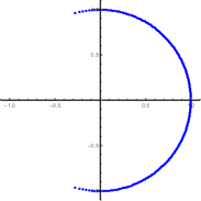
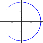
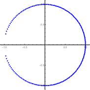
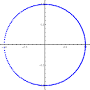
Figure 1. Zeroes of the unitary Hermite polynomials $H_{n}(z;\sigma^{2}/n)$ with $\sigma^{2}=1,2,3,4$. The degree is $n=200$.

The empirical distribution of zeroes of $H_{n}(z;\sigma^{2}/n)$ will be denoted by

$$\mu_{n;\sigma^{2}}:=\mu\lsem H_{n}(\,\cdot\,;\sigma^{2}/n)\rsem=\frac{1}{n}\sum_{z\in\mathbb{T}:\,H_{n}(z;\sigma^{2}/n)=0}\delta_{z}.$$ (2.2)

Theorem 2.2.

Fix some $\sigma^{2}>0$. Then, as $n\to\infty$, the probability measures $\mu_{n;\sigma^{2}}$ converge weakly on $\mathbb{T}$ to the free unitary normal distribution ${\mathfrak{N}}_{\sigma^{2}}$ with parameter $\sigma^{2}$; see Section 2.6 for its definition and properties.

One possible way to approach Theorem 2.2 is via the method of moments. Let $z_{1:n},\ldots,z_{n:n}$ be the zeroes of $H_{n}(z;\sigma^{2}/n)$ and let $p_{k,n}$ be the $k$-th moment of $\mu_{n;\sigma^{2}}$, that is

$$p_{k:n}:=\frac{1}{n}\sum_{j=1}^{n}z_{j:n}^{k}.$$

On the other hand, let $e_{k:n}$ be the $k$-th elementary symmetric polynomial of the zeroes, that is

$$e_{k:n}:=\sum_{1\leq j_{1}<\ldots<j_{k}\leq n}z_{j_{1}:n}\ldots z_{j_{k}:n}=\binom{n}{k}\exp\left\{-\frac{\sigma^{2}k(n-k)}{2n}\right\},$$

where the second equality follows from Vieta’s identities and (1.5). For every given $k\in\mathbb{N}$, we can express $p_{k:n}$ through $e_{1:n},\ldots,e_{k:n}$ using the Newton-Girard identities, write the binomial coefficients and the exponentials as series in powers of $n$ and $n^{-1}$, and compute the limit as $n\to\infty$. It turns out that the terms involving $n,\ldots,n^{k-1}$ cancel and the limit coincides with the $k$-th moment of ${\mathfrak{N}}_{\sigma^{2}}$ (for the latter, see Section 2.6). For example, for $k=3$ we have

$$p_{3:n}=\frac{1}{n}(e_{1:n}^{3}-3e_{1:n}e_{2:n}+3e_{3:n})\overset{}{\underset{n\to\infty}{\longrightarrow}}\frac{1}{2}{\rm e}^{-3\sigma^{2}/2}(2-6\sigma^{2}+3\sigma^{4})=\int_{\mathbb{T}}z^{3}{\mathfrak{N}}_{\sigma^{2}}(\textup{d}z).$$

Using computer algebra software, it is possible to check that $\lim_{n\to\infty}p_{k:n}=\int_{\mathbb{T}}z^{k}{\mathfrak{N}}_{\sigma^{2}}(\textup{d}z)$ for any given $k\in\mathbb{N}$, but we were unable to find a general proof of Theorem 2.2 based on this approach.

2.2. Asymptotics of unitary Hermite polynomials

Our asymptotic results on the polynomials $H_{n}(z;\sigma^{2}/n)$ will be stated in terms of certain analytic function $\zeta_{t}(\theta)$ that satisfies

$$\zeta_{t}(\theta)-t\tan\zeta_{t}(\theta)=\theta,$$

where $t>0$ is a parameter and $\theta$ is a complex variable satisfying $\operatorname{Im}\theta>0$. This function is related to the free unitary Poisson distribution, as has been shown in [41], and to the free unitary normal distribution, which will be demonstrated in Section 2.6 below. The next theorem summarizes the main properties of this function; see [41, Section 4] for proofs and further properties.

Theorem 2.3.

Fix $t>0$. Let $\mathbb{H}:=\{\theta\in\mathbb{C}:\,\operatorname{Im}\theta>0\}$ be the upper half-plane. For every $\theta\in\mathbb{H}$, the equation $\zeta-t\tan\zeta=\theta$ has a unique, simple solution $\zeta=\zeta_{t}(\theta)$ in $\mathbb{H}$. The function $\zeta_{t}:\mathbb{H}\to\mathbb{H}$ is analytic on $\mathbb{H}$, admits a continuous extension to the closed upper half-plane $\overline{\mathbb{H}}$, and satisfies

$$\zeta_{t}(\theta+\pi)=\zeta_{t}(\theta)+\pi,\qquad\zeta_{t}(-\bar{\theta})=-\overline{\zeta_{t}(\theta)},\qquad\operatorname{Im}\zeta_{t}(\theta)>\operatorname{Im}\theta,$$ (2.3)

for all $\theta\in\mathbb{H}$. Locally uniformly in $x\in\mathbb{H}$ we have

$$\zeta_{t}(\theta)=\lim_{n\to\infty}\underbrace{(\theta+t\tan(\theta+t\tan(\ldots(\theta+t\tan x)\ldots)))}_{n\text{ iterations}},\qquad\theta\in\overline{\mathbb{H}}.$$

Finally, we have

$$\zeta_{t}(\theta)-\theta\to{\rm{i}}t\quad\text{ as }\quad\operatorname{Im}\theta\to+\infty\quad\text{ uniformly in }\operatorname{Re}\theta\in\mathbb{R}.$$ (2.4)

The next theorem is our second main result.

Theorem 2.4.

Locally uniformly in $\theta\in\mathbb{H}$ we have

$$\lim_{n\to\infty}\frac{1}{n}\log\frac{H_{n}(-{\rm e}^{{\rm{i}}\theta};\sigma^{2}/n)}{(-1)^{n}}=\log\left(1+{\rm e}^{2{\rm{i}}\zeta_{\sigma^{2}/4}(\theta/2)}\right)-\frac{\sigma^{2}}{2\left(1+{\rm e}^{-2{\rm{i}}\zeta_{\sigma^{2}/4}(\theta/2)}\right)^{2}},$$ (2.5)

$$\lim_{n\to\infty}\frac{1}{n}\,\frac{H_{n}^{\prime}(-{\rm e}^{{\rm{i}}\theta};\sigma^{2}/n)}{H_{n}(-{\rm e}^{{\rm{i}}\theta};\sigma^{2}/n)}=\frac{-{\rm e}^{-{\rm{i}}\theta}}{1+{\rm e}^{-2{\rm{i}}\zeta_{\sigma^{2}/4}(\theta/2)}}=-{\rm e}^{-{\rm{i}}\theta}\left(\frac{{\rm{i}}}{2}\tan\zeta_{\sigma^{2}/4}(\theta/2)+\frac{1}{2}\right).$$ (2.6)

The logarithms in (2.5) are chosen such that $\log 1=0$ and all functions of the form $\log(\ldots)$ are continuous (and analytic) in $\theta\in\mathbb{H}$.

Remark 2.5.

We can consider all functions appearing in (2.5) and (2.6) as analytic functions of the variable $z:=-{\rm e}^{{\rm{i}}\theta}\in\mathbb{D}$ including the value $z=0$. Firstly, $z\to 0$ is equivalent to $\operatorname{Im}\theta\to+\infty$. In this regime, (2.4) implies that $\zeta_{\sigma^{2}/4}(\theta/2)=(\theta/2)+{\rm{i}}(\sigma^{2}/4)+o(1)$ and, consequently, $\operatorname{Im}\zeta_{\sigma^{2}/4}(\theta/2)\to+\infty$. It follows that the right-hand side of (2.5) converges to $0$, while the right-hand side of (2.6) converges to $-{\rm e}^{-\sigma^{2}/2}$. Secondly, note that $\theta$ corresponding to a given $z\in\mathbb{D}\backslash\{0\}$ is defined only up to a summand of the form $2\pi n$ with $n\in\mathbb{Z}$. Still, the right-hand sides of (2.5) and (2.6) stay invariant under the substitution $\theta\mapsto\theta+2\pi n$ (since $\zeta_{\sigma^{2}/4}(\theta/2+\pi n)=\zeta_{\sigma^{2}/4}(\theta/2)+\pi n$ by (2.3)) and hence define analytic functions of $z\in\mathbb{D}$. Analogous observations apply to many similar functions below. Note that convergence in (2.5) and (2.6) stays locally uniform in $z\in\mathbb{D}$. For $z$ outside any small disk around $0$, this is stated in Theorem 2.4, while the rest follows from Cauchy’s integration formula.

Remark 2.6.

Theorem 2.4 describes the asymptotics of $H_{n}(z;\sigma^{2}/n)$ for $|z|<1$. The asymptotics for $|z|>1$ can be derived from the identity $z^{n}H_{n}(1/z;\sigma^{2}/n)=(-1)^{n}H_{n}(z;\sigma^{2}/n)$ following from (1.5). On the circle $\{|z|=1\}$ one may expect an asymptotic result of Plancherel-Rotach type; see [63, Theorem 8.22.9] for the case of the classical Hermite polynomials.

2.3. Applications to the Curie-Weiss model

We are now going to describe the global limiting distribution of zeroes of $Z_{n}(\beta,h)$, the partition function of the Curie-Weiss model defined in (1.8). We consided the so-called Lee-Yang zeroes, that is we fix real $\beta>0$ and allow $h$ to be complex. By the Lee-Yang theorem, all zeroes are purely imaginary; see (1.9) and Lemma 2.1. Observe also that $Z_{n}(\beta,h+\pi{\rm{i}})={\rm e}^{\pi{\rm{i}}n}Z_{n}(\beta,h)$ by (1.8) implying that the zeros are periodic with period $\pi{\rm{i}}$.

Corollary 2.7.

Fix $\beta>0$. For the partition function of the Curie-Weiss model, the following convergence holds vaguely on $\mathbb{R}$:

$$\frac{1}{n}\sum_{y\in\mathbb{R}:\,Z_{n}(\beta,{\rm{i}}y)=0}\delta_{y}\overset{v}{\underset{n\to\infty}{\longrightarrow}}\nu_{\beta}.$$

Here, $\nu_{\beta}$ is a measure on $\mathbb{R}$ which is invariant under the shifts $h\mapsto h+\pi\ell$, $\ell\in\mathbb{Z}$, and is characterized by $\nu_{\beta}(A)={\mathfrak{N}}_{4\beta}(-{\rm e}^{2{\rm{i}}A})$ for every Borel set $A\subset(-\frac{\pi}{2},\frac{\pi}{2}]$, where ${\mathfrak{N}}_{4\beta}$ is the free unitary normal distribution on the unit circle with parameter $\sigma^{2}=4\beta$; see Section 2.6.

Proof.

Let $f:\mathbb{R}\to\mathbb{R}$ be a continuous function with compact support. Define $f^{*}(y):=\sum_{\ell\in\mathbb{Z}}f(y+\pi\ell)$ for $y\in(-\frac{\pi}{2},\frac{\pi}{2}]$. Let also $\psi:\mathbb{T}\to(-\frac{\pi}{2},\frac{\pi}{2}]$ be the inverse map of $y\mapsto-{\rm e}^{2{\rm{i}}y}$. Then, by (1.9),

$$\frac{1}{n}\sum_{y\in\mathbb{R}:\,Z_{n}(\beta,{\rm{i}}y)=0}f(y)=\frac{1}{n}\sum_{y\in(-\frac{\pi}{2},\frac{\pi}{2}]:\,H_{n}(-{\rm e}^{2{\rm{i}}y},\frac{4\beta}{n})=0}f^{*}(y)=\frac{1}{n}\sum_{z\in\mathbb{T}:\,H_{n}(z,\frac{4\beta}{n})=0}f^{*}(\psi(z)).$$

By Theorem 2.2, the latter sum converges to $\int_{\mathbb{T}}f^{*}(\psi(z)){\mathfrak{N}}_{4\beta}(\textup{d}z)=\int_{\mathbb{R}}f(y)\nu_{\beta}(\textup{d}y)$, and the claim follows. ∎

Remark 2.8.

The Lebesgue density of $\nu_{\beta}$ on $\mathbb{R}$ is given by $y\mapsto 2f_{4\beta}(-{\rm e}^{2{\rm{i}}y})=\frac{1}{\pi\beta}\operatorname{Im}\zeta_{\beta}(y)$, where $f_{4\beta}$ is the function which will be discussed in Theorem 2.16. It follows from this theorem that the support of $\nu_{\beta}$ is $\mathbb{R}$ for $\beta\geq 1$, while for $0<\beta<1$ the support is the union of the intervals

$$\left[\frac{\pi}{2}-\arcsin\sqrt{\beta}-\sqrt{\beta-\beta^{2}}+\pi\ell,\frac{\pi}{2}+\arcsin\sqrt{\beta}+\sqrt{\beta-\beta^{2}}+\pi\ell\right],\qquad\ell\in\mathbb{Z}.$$

If $\beta$ increases from $0$ to $\infty$, then the support of $\nu_{\beta}$ hits the real axis at $\beta=1$, which is well known to be the point of phase transition for the Curie-Weiss model.

In the next result we compute the free energy of the Curie-Weiss model in the complex $h$-plane excluding the imaginary axis.

Corollary 2.9.

Let $\beta>0$ and $h\in\mathbb{C}$ with $\operatorname{Re}h>0$. For the partition function of the Curie-Weiss model defined in (1.8) we have

$$\lim_{n\to\infty}\frac{1}{n}\log Z_{n}(\beta,h)=\lim_{n\to\infty}\frac{1}{n}\log Z_{n}(\beta,-h)=\frac{\beta}{2}+h+\log\left(1+{\rm e}^{2{\rm{i}}\zeta_{\beta}({\rm{i}}h)}\right)-\frac{2\beta}{\left(1+{\rm e}^{-2{\rm{i}}\zeta_{\beta}({\rm{i}}h)}\right)^{2}}.$$

Proof.

Recall that $Z_{n}(\beta,h)=Z_{n}(\beta,-h)$ is given by (1.8) and (1.9) and apply Theorem 2.4 with $\sigma^{2}=4\beta$ and $\theta=2{\rm{i}}h$. ∎

2.4. Expected characteristic polynomial of the Brownian motion on unitary matrices

It is well known [54, Section 6.1.2] that the expected characteristic polynomial of an $n\times n$ Wigner random matrix coincides with the $n$-th Hermite polynomial. Formulas of this type go back to Heine [63, Eqn. (2.2.11) on p. 27]. For this and analogous results on several other types of random matrices including the Wishart matrices whose expected characteristic polynomials are the Laguerre polynomials we refer to [54, Sections 6.2, 6.3], [5], [25, Chapter 9], [22, Theorem 4.1], [15, Eqn. (15)], [21, Proposition 12], [31, Proposition 11], [1, Theorem 1.1]. In this section we prove a similar result on unitary Hermite polynomials by relating them to the expected characteristic polynomials of the random matrices obtained by running a Brownian motion on the unitary group $U(n)$. More precisely, we consider the unitary group $U(n)$ as a compact Riemannian manifold endowed with the Riemannian metric induced by its natural embedding into $\mathbb{C}^{n\times n}\equiv\mathbb{R}^{2n^{2}}$. On the Lie algebra $\mathfrak{u}(n)=\{A\in\text{Mat}_{n\times n}(\mathbb{C}):A^{*}=-A\}$ (which can be identified with the tangent space of $U(n)$ at the identity matrix $I_{n}$) the scalar product takes the form $\langle A,B\rangle=\mathop{\mathrm{Tr}}\nolimits(AB^{*})=-\mathop{\mathrm{Tr}}\nolimits(AB)$. Let now $(U_{n}(t))_{t\geq 0}$ be the Brownian motion on the unitary group $U(n)$ starting at the identity matrix $I_{n}$ at time $t=0$. The eigenvalues $\lambda_{1}(t),\ldots,\lambda_{n}(t)$ of the unitary random matrix $U_{n}(t)$ represent a special case of Dyson’s Brownian motions [24, Section III] on the circle; see also [39, 18, 12, 37] for further information on this process.

To define Dyson’s Brownian motions on the circle, fix parameters $n\in\mathbb{N}$ and $\lambda>0$. Let $(B_{1}(t))_{t\geq 0},\ldots,(B_{n}(t))_{t\geq 0}$ be $n$ independent standard Brownian motions on $\mathbb{R}$. We are interested in real-valued stochastic processes $X_{1}(t)\leq\ldots\leq X_{n}(t)$, defined for $t\geq 0$ and solving stochastic differential equations

$$\textup{d}X_{j}=\textup{d}B_{j}+\lambda\cdot\bigg{(}\sum_{\begin{subarray}{c}k\in\{1,\ldots,n\}\\ k\neq j\end{subarray}}\cot\frac{X_{j}-X_{k}}{2}\Bigg{)}\textup{d}t,\qquad j=1,\ldots,n,$$ (2.7)

with the initial condition $X_{1}(0)=\ldots=X_{n}(0)=0$. If $\lambda=1/2$, then we can identify ${\rm e}^{{\rm{i}}X_{1}(t)},\ldots,{\rm e}^{{\rm{i}}X_{n}(t)}$ with the eigenvalues $\lambda_{1}(t),\ldots,\lambda_{n}(t)$ of the unitary random matrix $U_{n}(t)$. More precisely, it is known that the measure-valued process $(\sum_{\ell=1}^{n}\delta_{{\rm e}^{{\rm{i}}X_{\ell}(t)}})_{t\geq 0}$ has the same distribution as the process $(\sum_{\ell=1}^{n}\delta_{\lambda_{\ell}(t)})_{t\geq 0}$.

We are interested in the following polynomial in $x$ which, for $\lambda=1/2$, reduces to the characteristic polynomial of $U_{n}(t)$:

$$P_{n,\lambda}(x;t):=\prod_{j=1}^{n}\left(x-{\rm e}^{{\rm{i}}X_{j}(t)}\right).$$

Theorem 2.10.

For every $\lambda>0$, $n\in\mathbb{N}$, $t\geq 0$ and $x\in\mathbb{C}$ we have

$$\mathbb{E}P_{n,\lambda}(x;t)=\sum_{j=0}^{n}(-1)^{n-j}\binom{n}{j}{\rm e}^{-\frac{1}{2}(n-j)t-\lambda j(n-j)t}x^{j}={\rm e}^{-\frac{1}{2}nt}H_{n}({\rm e}^{t/2}x;2\lambda t).$$

Proof.

To simplify the notation, we shall usually suppress the dependence of quantities under consideration on $n$ and $\lambda$. Let $e_{\ell}(t)$ be the $\ell$-th elementary symmetric polynomial of ${\rm e}^{{\rm{i}}X_{1}(t)},\ldots,{\rm e}^{{\rm{i}}X_{n}(t)}$, that is

$$e_{\ell}(t)=\sum_{1\leq j_{1}<\ldots<j_{\ell}\leq n}{\rm e}^{{\rm{i}}X_{j_{1}}(t)+\ldots+{\rm{i}}X_{j_{\ell}}(t)},\qquad\ell=1,\ldots,n,$$

Put also $e_{0}(t)=1$. Since $P_{n,\lambda}(x;t)=\sum_{\ell=0}^{n}(-1)^{\ell}e_{\ell}(t)x^{n-\ell}$ by Vieta’s formula, it suffices to show that for all $\ell\in\{1,\ldots,n\}$ we have

$$\mathbb{E}e_{\ell}(t)=\binom{n}{\ell}{\rm e}^{-\frac{1}{2}\ell t-\lambda\ell(n-\ell)t}.$$

To this end, we shall derive stochastic differential equations satisfied by $e_{\ell}(t)$. Using the Itô formula, see, e.g., [55, Chapter IV, Theorem (3.3)], we have

$$\textup{d}e_{\ell}=\sum_{1\leq j_{1}<\ldots<j_{\ell}\leq n}\textup{d}\left({\rm e}^{{\rm{i}}X_{j_{1}}+\ldots+{\rm{i}}X_{j_{\ell}}}\right)=\sum_{1\leq j_{1}<\ldots<j_{\ell}\leq n}\left(\sum_{s=1}^{\ell}{\rm{i}}{\rm e}^{{\rm{i}}X_{j_{1}}+\ldots+{\rm{i}}X_{j_{\ell}}}\textup{d}X_{j_{s}}-\frac{\ell}{2}{\rm e}^{{\rm{i}}X_{j_{1}}+\ldots+{\rm{i}}X_{j_{\ell}}}\textup{d}t\right).$$

Write $V(x):=\lambda\cot\frac{x}{2}$. Recalling (2.7), we obtain

$$\textup{d}e_{\ell}=\sum_{1\leq j_{1}<\ldots<j_{\ell}\leq n}{\rm{i}}{\rm e}^{{\rm{i}}X_{j_{1}}+\ldots+{\rm{i}}X_{j_{\ell}}}\left(\textup{d}B_{j_{1}}+\ldots+\textup{d}B_{j_{\ell}}\right)-\frac{\ell}{2}e_{\ell}\textup{d}t+R\textup{d}t$$ (2.8)

with

$$R :=\sum_{1\leq j_{1}<\ldots<j_{\ell}\leq n}{\rm{i}}{\rm e}^{{\rm{i}}X_{j_{1}}+\ldots+{\rm{i}}X_{j_{\ell}}}\Bigg{(}\sum_{\begin{subarray}{c}m\in\{1,\ldots,n\}\\ m\neq j_{1}\end{subarray}}V(X_{j_{1}}-X_{m})+\ldots+\sum_{\begin{subarray}{c}m\in\{1,\ldots,n\}\\ m\neq j_{\ell}\end{subarray}}V(X_{j_{\ell}}-X_{m})\Bigg{)}$$

$$=\sum_{1\leq j_{1}<\ldots<j_{\ell}\leq n}{\rm{i}}{\rm e}^{{\rm{i}}X_{j_{1}}+\ldots+{\rm{i}}X_{j_{\ell}}}\Bigg{(}\sum_{m\in\{1,\ldots,n\}\backslash\{j_{1},\ldots,j_{\ell}\}}\Big{(}V(X_{j_{1}}-X_{m})+\ldots+V(X_{j_{\ell}}-X_{m})\Big{)}\Bigg{)},$$

where in the second line we used that $V(-x)=-V(x)$. After some re-indexing, we can write

$$R =\frac{{\rm{i}}}{(\ell+1)!}\sum_{\begin{subarray}{c}k_{0},\ldots,k_{\ell}\in\{1,\ldots,n\}\\ \text{pairwise distinct}\end{subarray}}{\rm e}^{{\rm{i}}X_{k_{0}}+{\rm{i}}X_{k_{1}}+\ldots+{\rm{i}}X_{k_{\ell}}}\sum_{\begin{subarray}{c}s,p\in\{0,\ldots,\ell\}\\ s\neq p\end{subarray}}\frac{V(X_{k_{p}}-X_{k_{s}})}{{\rm e}^{{\rm{i}}X_{k_{s}}}}$$

$$=\frac{{\rm{i}}}{2(\ell+1)!}\sum_{\begin{subarray}{c}k_{0},\ldots,k_{\ell}\in\{1,\ldots,n\}\\ \text{pairwise distinct}\end{subarray}}{\rm e}^{{\rm{i}}X_{k_{0}}+{\rm{i}}X_{k_{0}}+\ldots+{\rm{i}}X_{k_{\ell}}}\sum_{\begin{subarray}{c}s,p\in\{0,\ldots,\ell\}\\ s\neq p\end{subarray}}\left(\frac{V(X_{k_{p}}-X_{k_{s}})}{{\rm e}^{{\rm{i}}X_{k_{s}}}}+\frac{V(X_{k_{s}}-X_{k_{p}})}{{\rm e}^{{\rm{i}}X_{k_{p}}}}\right).$$

To simplify the expression in the brackets, note that

$$\frac{V(x-y)}{{\rm e}^{{\rm{i}}y}}+\frac{V(y-x)}{{\rm e}^{{\rm{i}}x}}=\lambda\cot\left(\frac{x-y}{2}\right)\left({\rm e}^{{\rm{i}}(x-y)}-1\right){\rm e}^{-{\rm{i}}x}={\rm{i}}\lambda\left({\rm e}^{-{\rm{i}}x}+{\rm e}^{-{\rm{i}}y}\right).$$

It follows that

$$R =\frac{-\lambda}{2(\ell+1)!}\sum_{\begin{subarray}{c}k_{0},\ldots,k_{\ell}\in\{1,\ldots,n\}\\ \text{pairwise distinct}\end{subarray}}{\rm e}^{{\rm{i}}X_{k_{0}}+{\rm{i}}X_{k_{1}}+\ldots+{\rm{i}}X_{k_{\ell}}}\sum_{\begin{subarray}{c}s,p\in\{0,\ldots,\ell\}\\ s\neq p\end{subarray}}\left({\rm e}^{-{\rm{i}}X_{k_{s}}}+{\rm e}^{-{\rm{i}}X_{k_{p}}}\right)$$

$$=-\lambda\ell(n-\ell)e_{\ell}(t).$$

To justify the last identity, observe that the double sum in the first line must be a multiple of $e_{\ell}$ for symmetry reasons and that it contains $(n)_{\ell+1}\cdot(\ell+1)\ell\cdot 2$ summands, while $e_{\ell}$ contains $\binom{n}{\ell}$ summands. Taking the quotient of these two numbers, it follows that the double sum in the first line equals $2(\ell+1)!\ell(n-\ell)e_{\ell}$. Finally, recalling (2.8), we arrive at the stochastic differential equation

$$\textup{d}e_{\ell}=-\left(\frac{\ell}{2}+\lambda\ell(n-\ell)\right)e_{\ell}\textup{d}t+\sum_{j=1}^{n}{\rm{i}}{\rm e}^{{\rm{i}}X_{j}}e_{\ell-1}^{(j)}\textup{d}B_{j},$$ (2.9)

where $e_{\ell-1}^{(j)}$ is the $(\ell-1)$-st elementary symmetric polynomial of ${\rm e}^{{\rm{i}}X_{1}},\ldots,{\rm e}^{{\rm{i}}X_{j-1}},{\rm e}^{{\rm{i}}X_{j+1}},\ldots,{\rm e}^{{\rm{i}}X_{n}}$ (excluding ${\rm e}^{{\rm{i}}X_{j}}$). From the Itô formula it follows that ${\rm e}^{\frac{1}{2}\ell t+\lambda\ell(n-\ell)t}e_{\ell}(t)$ is a martingale. Recalling that $e_{\ell}(0)=\binom{n}{\ell}$ we conclude that

$$\mathbb{E}e_{\ell}(t)=\binom{n}{\ell}{\rm e}^{-\frac{1}{2}\ell t-\lambda\ell(n-\ell)t},$$

and the proof is complete. ∎

Biane [10, 11] proved that, as $n\to\infty$, the process $(U_{n}(t/n))_{t\geq 0}$ converges (in a suitable sense) to the free unitary Brownian motion. In particular, by [10, Theorem 1], the spectral distribution of $U_{n}(t/n)$ converges weakly the free unitary normal distribution ${\mathfrak{N}}_{t}$ (making the appearance of this distribution in Theorem 2.2 quite natural); see also [16, Section 3.3] for related large deviation results. Exact combinatorial formulas for moments of the form $\mathbb{E}[\mathop{\mathrm{Tr}}\nolimits(U_{n}^{m_{1}}(t))\ldots\mathop{\mathrm{Tr}}\nolimits(U_{n}^{m_{r}}(t))]$ have been derived in [47].

2.5. The action of the backward heat flow on the roots

Consider a sequence of polynomials (or trigonometric polynomials) of increasing degrees whose empirical distributions of roots approach some probability measure. One may ask what happens to the asymptotic distribution of roots if we apply to these polynomials certain operator. One special case, in which the operator is the repeated differentiation, has been studied in [60, 61, 62, 53, 40, 14, 43, 7, 41, 33]. For trigonometric polynomials, it has been shown in [41] that, on the level of roots, the repeated differentiation induces the free unitary Poisson process. In his blog, Tao [64, 65] discusses the evolution of zeroes of a polynomial which undergoes a (backward) heat flow. As this paper was almost complete, Jonas Jalowy brought to our attention the recent preprint by Hall and Ho [38] who studied the action of the backward heat flow on the characteristic polynomials of the Ginibre matrices (whose eigenvalues obey the circular law). We shall consider two settings: algebraic polynomials and trigonometric polynomials, both with real roots, and show that the backward heat flow induces free (additive or unitary) Brownian motion on the level of roots.

Heat flow acting on algebraic polynomials

Let $(P_{n}(z))_{n\in\mathbb{N}}$ be a sequence of algebraic polynomials from $\mathbb{R}[z]$. We suppose that $P_{n}(z)=\sum_{j=0}^{n}a_{j:n}z^{j}$ is real-rooted (that is, it has only real roots) and that all roots are contained in some fixed interval $[-C,C]$ with $C$ not depending on $n$. Moreover, we suppose that the empirical distribution of roots of $P_{n}$ converges weakly to some probability measure $\mu$ on $[-C,C]$, that is

$$\mu\lsem P_{n}\rsem=\frac{1}{n}\sum_{\begin{subarray}{c}z\in\mathbb{R}:\,P_{n}(z)=0\end{subarray}}\delta_{z}\overset{w}{\underset{n\to\infty}{\longrightarrow}}\mu.$$ (2.10)

The roots are counted with multiplicities, as always. We are interested in the action which the backward heat flow induces on the roots of $P_{n}$, in the large $n$ limit. More precisely, we consider the heat equation on the real line with initial condition given by $P_{n}(z)$:

$$\partial_{t}g_{n}(z;t)=\frac{1}{2}\partial^{2}_{z}g_{n}(z;t),\qquad g_{n}(z;0)=P_{n}(z),\qquad z\in\mathbb{R},\;t\in\mathbb{R}.$$ (2.11)

The solution is explicit and can be written as

$$g_{n}(z;-s)={\rm e}^{-\frac{s}{2}\partial_{z}^{2}}P_{n}(z)=\sum_{j=0}^{n}a_{j:n}{\rm e}^{-\frac{s}{2}\partial_{z}^{2}}z^{j}=\sum_{j=0}^{n}a_{j:n}\mathop{\mathrm{He}}\nolimits_{j}\left(\frac{z}{\sqrt{s}}\right)s^{j/2},\qquad z\in\mathbb{R},\;s\in\mathbb{R},$$ (2.12)

where $\mathop{\mathrm{He}}\nolimits_{j}(z)$ is the $j$-th probabilist Hermite polynomial defined by (1.1) or (1.2). Note that the solution exists both for positive and negative times since the term $\mathop{\mathrm{He}}\nolimits_{j}(z/\sqrt{s})s^{j/2}$ does not contain fractional powers of $s$, see (1.1), and makes sense irrespective of the sign of $s$. Moreover, for every $s\in\mathbb{R}$, the function $z\mapsto g_{n}(z;-s)$ is a polynomial. In the sequel, we shall focus on the case $s>0$, which corresponds to the backward heat equation. It is known to be ill-posed for initial conditions more general than polynomials. Since we assume that the initial condition $P_{n}(z)$ is real-rooted, the polynomials $g_{n}(z;-s)$ remain real-rooted for all $s\geq 0$ by the Pólya-Benz theorem; see [8] or [2, Theorem 1.2]. Another proof of this fact can be found [64].

Theorem 2.11.

Fix $r>0$. Under the above assumptions, the empirical distribution of zeroes of the polynomials $g_{n}(z;-r^{2}/n)$ converges weakly (as $n\to\infty$) to the free additive convolution $\mu\boxplus\gamma_{0,2r}$ of $\mu$ and the Wigner semicircle distribution $\gamma_{0,2r}$ with density $x\mapsto\frac{1}{2\pi r^{2}}\sqrt{4r^{2}-x^{2}}$ on the interval $[-2r,2r]$.

To prove this theorem, we shall use a result from finite free probability [48, 49]. Recall from (1.6) the definition of the finite free additive convolution $\boxplus_{n}$. It is known from [6, Corollary 5.5 and Theorem 5.4], see also [48, Theorem 4.3], that, as $n\to\infty$, the finite free additive convolution $\boxplus_{n}$ approaches the free additive convolution $\boxplus$ in the following sense.

Proposition 2.12.

Let $(p_{n})_{n\in\mathbb{N}}$ and $(q_{n})_{n\in\mathbb{N}}$ be sequences of polynomials in $\mathbb{R}[z]$ whose roots are contained in some fixed interval $[-C,C]$. Suppose that $\deg p_{n}=\deg q_{n}=n$ and the empirical distributions of zeroes of $p_{n}$ and $q_{n}$ converge weakly to certain probability measures $\nu$ and $\rho$ on $[-C,C]$. Then, the empirical distribution of zeroes of $p_{n}\boxplus_{n}q_{n}$ (which is also real-rooted by [49, Theorem 1.3]) converges weakly to $\nu\boxplus\rho$.

Indeed, $\mu\lsem p_{n}\rsem\to\nu$ and $\mu\lsem q_{n}\rsem\to\rho$ (weakly) implies that the moments of $\mu\lsem p_{n}\rsem$ and $\mu\lsem q_{n}\rsem$ converge to the corresponding moments of $\nu$ and $\rho$ (since all measures are concentrated on a fixed interval). By the results cited above, this implies that the moments of the empirical distribution of zeroes of $p_{n}\boxplus_{n}q_{n}$ converge to those of $\nu\boxplus\rho$. This implies that the probability measures $\mu\lsem p_{n}\boxplus_{n}q_{n}\rsem$ (which are concentrated on $[-2C,2C]$ by [49, Theorem 1.3]) converge weakly to $\nu\boxplus\rho$.

Proof of Theorem 2.11..

It is known [49] that $\boxplus_{n}$ commutes with differentiation in the sense that $\partial_{z}(p(z)\boxplus_{n}q(z))=(\partial_{z}p(z))\boxplus_{n}q(z)$ for arbitrary polynomials $p(z)$ and $q(z)$ of degree at most $n$. By bilinearity of $\boxplus_{n}$ it follows that it also commutes with the operator $\exp\{-\frac{s}{2}\partial_{z}^{2}\}$, for all $s\in\mathbb{R}$. Hence,

$$g_{n}(z;-s)={\rm e}^{-\frac{s}{2}\partial_{z}^{2}}P_{n}(z)={\rm e}^{-\frac{s}{2}\partial_{z}^{2}}\left(P_{n}(z)\boxplus_{n}z^{n}\right)=P_{n}(z)\boxplus_{n}\left({\rm e}^{-\frac{s}{2}\partial_{z}^{2}}z^{n}\right)=P_{n}(z)\boxplus_{n}\mathop{\mathrm{He}}\nolimits_{n}\left(\frac{z}{\sqrt{s}}\right)s^{n/2},$$

where we used (1.2) in the last equality. We take $s=r^{2}/n$ and let $n\to\infty$. By a classical result, the empirical distribution of zeroes of the Hermite polynomial $\mathop{\mathrm{He}}\nolimits_{n}(z\sqrt{n}/r)$ converges weakly to the Wigner distribution with the density $x\mapsto\frac{1}{2\pi r^{2}}\sqrt{4r^{2}-x^{2}}$ on the interval $[-2r,2r]$; see, e.g., [66, 34, 44]. Applying Proposition 2.12 completes the proof. ∎

Remark 2.13.

Tao [64] derived the following system of differential equations satisfied by the roots $z_{1:n}(s),\ldots,z_{n:n}(s)$ of the polynomial $g_{n}(z;-s)$:

$$\partial_{s}z_{i:n}(s)=\sum_{\begin{subarray}{c}k\in\{1,\ldots,n\}\\ k\neq i\end{subarray}}\frac{1}{z_{i:n}(s)-z_{k:n}(s)},\qquad i=1,\ldots,n,$$ (2.13)

and proved that the solutions are well-defined for $s\geq 0$ but may run into a singularity for $s\leq 0$. These equations are Dyson’s Brownian motions with vanishing variance (or with $\beta=\infty$); see [3, Theorem 4.3.2]. Therefore, one can view Theorem 2.11 as the $\beta=\infty$ case of [3, Proposition 4.3.10]. For other results relating Dyson’s Brownian motions to free convolutions we refer to [4, 23, 36, 70, 71].

Heat flow acting on trigonometric polynomials

Let us now state analogous results for trigonometric polynomials. For every even number $n=2d$, $d\in\mathbb{N}$, let $T_{n}(\theta):=\sum_{\ell=-d}^{d}c_{\ell:n}{\rm e}^{{\rm{i}}\ell\theta}$ be a trigonometric polynomial with complex coefficients $c_{\ell:n}$ satisfying $c_{-\ell:n}=\overline{c_{\ell:n}}$ for all $\ell\in\{-d,\ldots,d\}$ (meaning that $T_{n}(\theta)$ takes real values for real $\theta$). Moreover, assume that $T_{n}(\theta)$ is real-rooted meaning that it has $n$ real roots $\theta_{1;n},\ldots,\theta_{n;n}$ (counting multiplicities) and that its empirical distribution of zeroes converges weakly as $n\to\infty$. The latter assumption will be written in the following form:

$$\nu\lsem T_{n}\rsem:=\frac{1}{n}\sum_{j=1}^{n}\delta_{{\rm e}^{{\rm{i}}\theta_{j;n}}}\overset{w}{\underset{n\to\infty}{\longrightarrow}}\nu$$ (2.14)

weakly on the unit circle $\mathbb{T}$, for some probability measure $\nu$ on $\mathbb{T}$. Consider the heat equation on the real line with periodic initial condition given by $T_{n}(\theta)$:

$$\partial_{t}f_{n}(\theta;t)=\frac{1}{2}\partial^{2}_{\theta}f_{n}(\theta;t),\qquad f_{n}(\theta;0)=T_{n}(\theta),\qquad\theta\in\mathbb{R},\;t\in\mathbb{R}.$$ (2.15)

Its solution is explicit and can be written as

$$f_{n}(\theta;t)={\rm e}^{\frac{t}{2}\partial_{\theta}^{2}}T_{n}(\theta)=\sum_{\ell=-d}^{d}c_{\ell:n}{\rm e}^{\frac{t}{2}\partial_{\theta}^{2}}{\rm e}^{{\rm{i}}\ell\theta}=\sum_{\ell=-d}^{d}c_{\ell:n}{\rm e}^{-\frac{t}{2}\ell^{2}}{\rm e}^{{\rm{i}}\ell\theta}.$$ (2.16)

For every $t\in\mathbb{R}$, the function $\theta\mapsto f_{n}(\theta;t)$ is a trigonometric polynomial. In particular, the solution makes sense both for $t\geq 0$ and for $t<0$. In the sequel we shall focus on the latter case, which corresponds to the backward heat equation. For $s>0$, the trigonometric polynomial $f_{n}(\theta;-s)$ remains real-rooted. This claim can be deduced from the Pólya-Benz theorem [2, Corollary 1.3]. Another proof can be found in [65] (where differential equations analogous to (2.13) in the circular setting are derived; see also [18, 39] for the corresponding stochastic differential equations).

Theorem 2.14.

Take some $\sigma^{2}>0$. In the setting described above, including Assumption (2.14), the empirical distribution $\nu\lsem f_{n}(\cdot\,;-\sigma^{2}/n)\rsem$ of zeroes of the solution $f_{n}(\theta;-\sigma^{2}/n)$ of the heat equation at time $t_{n}:=-\sigma^{2}/n$, converges weakly (as $n=2d\to\infty$) to the free unitary convolution $\nu\boxtimes{\mathfrak{N}}_{\sigma^{2}}$ of $\nu$ and the free unitary normal distribution ${\mathfrak{N}}_{\sigma^{2}}$.

We again rely on a result from finite free probability [49, 48]. Recall from (1.7) the definition of the finite free multiplicative convolution $\boxtimes_{n}$. The following fact proved in [7, Proposition 3.4] (see also [41, Proposition 2.9] for the version stated here) states that, in a suitable sense, $\boxtimes_{n}$ converges to the free multiplicative convolution $\boxtimes$ as $n\to\infty$.

Proposition 2.15.

Let $(p_{n}(z))_{n\in\mathbb{N}}$ and $(q_{n}(z))_{n\in\mathbb{N}}$ be sequences of polynomials in $\mathbb{C}[z]$ with $\deg p_{n}=\deg q_{n}=n$. Suppose that all roots of $p_{n}$ and $q_{n}$ are located on the unit circle and that, as $n\to\infty$, the empirical distributions of zeroes $\mu\lsem p_{n}\rsem$ and $\mu\lsem q_{n}\rsem$ converge weakly to two probability measures $\nu$ and $\rho$ on $\mathbb{T}$. Then, all roots of the polynomial $p_{n}\boxtimes_{n}q_{n}$ are also located on $\mathbb{T}$ and $\mu\lsem p_{n}\boxtimes_{n}q_{n}\rsem$ converges weakly to $\nu\boxtimes\rho$.

Proof of Theorem 2.14..

For $t\in\mathbb{R}$ we consider the algebraic polynomial $P_{2d}(z;t)$ in the complex variable $z$ defined by

$$\frac{P_{2d}({\rm e}^{{\rm{i}}\theta};t)}{{\rm e}^{{\rm{i}}d\theta}}=f_{2d}(\theta;t),$$ (2.17)

More concretely, it follows from (2.16) that

$$P_{2d}(z;t)=\sum_{\ell=-d}^{d}c_{\ell:2d}{\rm e}^{-\frac{t}{2}\ell^{2}}z^{\ell+d}=\sum_{j=0}^{2d}c_{j-d:2d}{\rm e}^{-\frac{t}{2}(j-d)^{2}}z^{j}=\sum_{j=0}^{2d}c_{j-d:2d}{\rm e}^{-\frac{t}{2}(j^{2}-2jd+d^{2})}z^{j}.$$

It follows from (1.7) and (1.5) that for $t=t_{2d}=-\sigma^{2}/(2d)<0$ we can write

$$P_{2d}(z;t) ={\rm e}^{-\frac{td^{2}}{2}}\left(\sum_{j=0}^{2d}(-1)^{2d-j}\binom{2d}{j}{\rm e}^{\frac{t}{2}j(2d-j)}z^{j}\right)\boxtimes_{2d}\left(\sum_{j=0}^{2d}c_{j-d:2d}z^{j}\right)$$

$$={\rm e}^{-\frac{td^{2}}{2}}\left(H_{2d}\left(z;\frac{\sigma^{2}}{2d}\right)\boxtimes_{2d}P_{2d}(z;0)\right).$$

Recall from Theorem 2.2 that the empirical distribution of zeroes of $H_{2d}(z;\sigma^{2}/(2d))$ converges weakly to ${\mathfrak{N}}_{\sigma^{2}}$, while the empirical distribution of zeroes of $P_{2d}(z;0)$ converges to $\nu$ by (2.17) and (2.14):

$$\frac{1}{2d}\sum_{\begin{subarray}{c}z\in\mathbb{C}:\,H_{2d}(z;\sigma^{2}/(2d))=0\end{subarray}}\delta_{z}\overset{w}{\underset{d\to\infty}{\longrightarrow}}{\mathfrak{N}}_{\sigma^{2}},\qquad\frac{1}{2d}\sum_{\begin{subarray}{c}z\in\mathbb{C}:\,P_{2d}(z;0)=0\end{subarray}}\delta_{z}=\frac{1}{2d}\sum_{j=1}^{2d}\delta_{{\rm e}^{{\rm{i}}\theta_{j;2d}}}\overset{w}{\underset{d\to\infty}{\longrightarrow}}\nu.$$

To complete the proof, apply Proposition 2.15. ∎

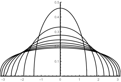
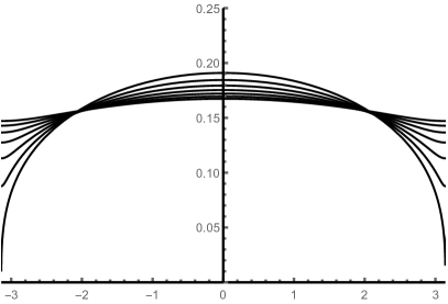
Figure 2. Densities of the free unitary normal distributions ${\mathfrak{N}}_{\sigma^{2}}$. The plots show the functions $\theta\mapsto f_{\sigma^{2}}({\rm e}^{{\rm{i}}\theta})$ for $\theta\in[-\pi,\pi]$. Left: $\sigma^{2}=0.5,1,1.5,\ldots,4$. Right: $\sigma^{2}=4,4.5,5,\ldots,7$.

2.6. Free unitary normal distribution and its properties

In this section we recall the notion of free multiplicative convolution $\boxtimes$ of probability measures on the unit circle which was introduced by Voiculescu in [67] and [68]; see also [69, § 3.6]. Also, we recall the definition of the free unitary normal distribution, which was introduced by Bercovici and Voiculescu [9] and studied in [10, 11, 73, 74, 17]. Finally, we shall state some properties of this distribution.

Given two probability measures $\mu_{1}$ and $\mu_{2}$ on the unit circle $\mathbb{T}$, it is possible to construct a $C^{*}$-probability space and two mutually free unitaries $u_{1}$ and $u_{2}$ with spectral distributions $\mu_{1}$ and $\mu_{2}$, respectively. Then, the free multiplicative convolution of $\mu_{1}$ and $\mu_{2}$, denoted by $\mu_{1}\boxtimes\mu_{2}$, is the spectral distribution of $u_{1}u_{2}$. It does not depend on the choice of $u_{1}$ and $u_{2}$; see [69] for more details. Free multiplicative convolution is linearized by the $S$-transform which is defined as follows. The $\psi$-transform of a probability measure $\mu$ on the unit circle $\mathbb{T}$ is defined by

$$\psi_{\mu}(z)=\int_{\mathbb{T}}\frac{uz}{1-uz}\mu(\textup{d}u)=\sum_{\ell=1}^{\infty}z^{\ell}\int_{\mathbb{T}}u^{\ell}\mu(\textup{d}u),\qquad z\in\mathbb{D}.$$ (2.18)

If $\psi_{\mu}^{\prime}(0)=\int_{\mathbb{T}}u\mu(\textup{d}u)\neq 0$, then the analytic function $\psi_{\mu}$ has an inverse on some sufficiently small disk around the origin and the $S$-transform of $\mu$ is defined by

$$S_{\mu}(z)=\frac{1+z}{z}\psi^{-1}_{\mu}(z).$$ (2.19)

The free unitary normal distribution ${\mathfrak{N}}_{\sigma^{2}}$ with parameter $\sigma^{2}>0$ introduced in [9, Lemmas 6.3], is a probability measure on $\mathbb{T}$ with

$$S_{{\mathfrak{N}}_{\sigma^{2}}}(z)={\rm e}^{\sigma^{2}(z+\frac{1}{2})}.$$ (2.20)

The next theorem summarizes some properties of the free unitary normal distributions; see Figure 2 for the plots of their densities. Almost all of these properties are known from the work of Biane [10], [11, Proposition 10]; see also the discussion in [42, Proposition 2.24] and [47, Remark 6.8] for further pointers to the literature. For similar properties of the free unitary Poisson distribution we refer to [41, Section 5].

Theorem 2.16.

The density of the free unitary normal distribution ${\mathfrak{N}}_{\sigma^{2}}$ w.r.t. the length measure on $\mathbb{T}$ is given by

$$f_{\sigma^{2}}({\rm e}^{{\rm{i}}\theta})=\frac{2}{\pi\sigma^{2}}\operatorname{Im}\zeta_{\sigma^{2}/4}\left(\frac{\theta-\pi}{2}\right),\qquad\theta\in\mathbb{R},$$ (2.21)

where $\zeta_{\sigma^{2}/4}(\cdot)$ is the function appearing in Theorem 2.3. The distribution ${\mathfrak{N}}_{\sigma^{2}}$ is invariant under complex conjugation meaning that $f_{\sigma^{2}}({\rm e}^{{\rm{i}}\theta})=f_{\sigma^{2}}({\rm e}^{-{\rm{i}}\theta})$.

• For $\sigma^{2}>4$, the function $\theta\mapsto f_{\sigma^{2}}({\rm e}^{{\rm{i}}\theta})$ is strictly positive and real analytic on $\mathbb{R}$.

• For $0<\sigma^{2}<4$, the function $\theta\mapsto f_{\sigma^{2}}({\rm e}^{{\rm{i}}\theta})$ is continuous on its period $[-\pi,\pi]$. It is strictly positive and real-analytic on the interval $(-m_{\sigma^{2}},+m_{\sigma^{2}})$, and vanishes on its complement $[-\pi,\pi]\backslash(-m_{\sigma^{2}},+m_{\sigma^{2}})$, where

  $$m_{\sigma^{2}}:=2\arcsin\frac{\sigma}{2}+\frac{\sigma}{2}\sqrt{4-\sigma^{2}}=\int_{0}^{\sigma}\sqrt{4-t^{2}}\,\textup{d}t.$$ (2.22)

  At the points $\pm m_{\sigma^{2}}$, the function $\theta\mapsto f_{\sigma^{2}}({\rm e}^{{\rm{i}}\theta})$ vanishes and has square-root singularities with

  $$f_{\sigma^{2}}({\rm e}^{{\rm{i}}(m_{\sigma^{2}}-\varepsilon)})=f_{\sigma^{2}}({\rm e}^{{\rm{i}}(\varepsilon-m_{\sigma^{2}})})\sim\frac{1}{\pi\sigma^{2}}\sqrt[4]{\frac{4\sigma^{2}}{4-\sigma^{2}}}\cdot\sqrt{\varepsilon},\qquad\varepsilon\downarrow 0.$$ (2.23)

• For $\sigma^{2}=4$, the function $\theta\mapsto f_{\sigma^{2}}({\rm e}^{{\rm{i}}\theta})$ is strictly positive and real-analytic on the interval $(-\pi,\pi)$. At $\theta=\pm\pi$, it vanishes and has cubic-root singularities with

  $$f_{\sigma^{2}}({\rm e}^{{\rm{i}}(\pi-\varepsilon)})=f_{\sigma^{2}}({\rm e}^{{\rm{i}}(\varepsilon-\pi)})\sim\frac{\sqrt{3}}{4\pi}\left(\frac{3\varepsilon}{2}\right)^{1/3},\qquad\varepsilon\downarrow 0.$$ (2.24)

Proof of Theorem 2.16.

We shall show in Lemma 3.3 below that

$$\psi_{{\mathfrak{N}}_{\sigma^{2}}}(-{\rm e}^{{\rm{i}}\theta})=\frac{{\rm{i}}\left(\theta-2\zeta_{\sigma^{2}/4}(\theta/2)\right)}{\sigma^{2}}-\frac{1}{2},\qquad\theta\in\mathbb{H}.$$

Consider the Poisson integral of ${\mathfrak{N}}_{\sigma^{2}}$ given for $z\in\mathbb{D}$ by

$$F_{{\mathfrak{N}}_{\sigma^{2}}}(z):=\frac{1}{2\pi}\operatorname{Re}\int_{\mathbb{T}}\frac{u+z}{u-z}\,{\mathfrak{N}}_{\sigma^{2}}({\rm d}u)=\frac{1}{2\pi}\operatorname{Re}\int_{\mathbb{T}}\frac{1+z\bar{u}}{1-z\bar{u}}\,{\mathfrak{N}}_{\sigma^{2}}({\rm d}u)=\frac{1}{2\pi}\operatorname{Re}(1+2\psi_{{\mathfrak{N}}_{\sigma^{2}}}(\bar{z})).$$

Since the function $\zeta_{\sigma^{2}/4}$ admits a continuous extension to $\overline{\mathbb{H}}$, the above formula defines $F_{{\mathfrak{N}}_{\sigma^{2}}}(z)$ as a continuous function on $\overline{\mathbb{D}}$. Under these circumstances, it is well known (see, e.g., [41, Lemma 5.2]) that the density of ${\mathfrak{N}}_{\sigma^{2}}$ with respect to the length measure on $\mathbb{T}$ is given by

$$f_{\sigma^{2}}({\rm e}^{{\rm{i}}\theta})=F_{{\mathfrak{N}}_{\sigma^{2}}}({\rm e}^{{\rm{i}}\theta})=\frac{1}{2\pi}\operatorname{Re}(1+2\psi_{{\mathfrak{N}}_{\sigma^{2}}}({\rm e}^{-{\rm{i}}\theta}))=\frac{1}{2\pi}\operatorname{Re}(1+2\psi_{{\mathfrak{N}}_{\sigma^{2}}}(-{\rm e}^{{\rm{i}}(\pi-\theta})))=\frac{2}{\pi\sigma^{2}}\operatorname{Im}\zeta_{\sigma^{2}/4}\left(\frac{\theta-\pi}{2}\right)$$

for all $\theta\in\mathbb{R}$. All other claims follow from the properties of the function $\zeta_{\sigma^{2}/4}$ derived in [41, Section 4]. In particular, Equation (2.23) follows from (2.21) and [41, Remark 4.3], while Equation (2.24) is a consequence of [41, Lemma 4.5]. ∎

Remark 2.17.

It follows from (2.21) and the series expansion of $\zeta_{\sigma^{2}/4}$ given in [41, Theorem 4.11] that

$$f_{\sigma^{2}}({\rm e}^{{\rm{i}}\theta})=\frac{1}{2\pi}+\frac{1}{\pi}\sum_{\ell=1}^{\infty}\frac{1}{\ell}{\rm e}^{-\ell\sigma^{2}/2}q_{\ell-1}(-\ell\sigma^{2})\cos(\ell\theta),$$ (2.25)

where $q_{m}(x)=\sum_{j=0}^{m}\frac{x^{j}}{j!}\binom{m+1}{j+1}$, $m\in\mathbb{N}_{0}$, and the series converges uniformly in $\theta\in\mathbb{R}$. Note that (2.25) characterizes the moments of ${\mathfrak{N}}_{\sigma^{2}}$. In this form, the result be found in [10, Lemma 1].

Remark 2.18.

A function very similar to $m_{\sigma^{2}}$ appears in [56, Theorem 5.1].

It follows from (2.25) that, as $\sigma^{2}\to\infty$, the density $f_{\sigma^{2}}({\rm e}^{{\rm{i}}\theta})$ converges to $1/(2\pi)$ uniformly, which implies that the free unitary normal distribution converges to the uniform distribution weakly on $\mathbb{T}$. On the other hand, the next result states that, as $\sigma^{2}\to 0$, the free unitary normal distribution ${\mathfrak{N}}_{\sigma^{2}}$ can be approximated by a Wigner semicircle distribution supported on a small arc of length $\sim 4\sigma$ centered at $1$.

Proposition 2.19.

For all $x\in(-2,2)$ we have $\lim_{\sigma^{2}\downarrow 0}\sigma f_{\sigma^{2}}({\rm e}^{{\rm{i}}\sigma x})=\frac{1}{2\pi}\sqrt{4-x^{2}}$.

Proof.

We shall only sketch the idea without giving full details. First of all, from (2.22) we have $m_{\sigma^{2}}\sim 2\sigma$ as $\sigma^{2}\downarrow 0$. Let us take $x=0$. It has been argued in [41, Section 4] that for all $\tau\geq 0$, we have $\zeta_{\sigma^{2}/4}(-\frac{\pi}{2}+{\rm{i}}\tau)=-\frac{\pi}{2}+{\rm{i}}\tilde{y}_{\sigma^{2}/4}(\tau)$, where $\tilde{y}=\tilde{y}_{\sigma^{2}/4}(\tau)>0$ is the unique positive solution of $\tilde{y}-\frac{1}{4}\sigma^{2}\operatorname*{cotanh}\tilde{y}=\tau$. For $\tau=0$ the equation takes the form $\tilde{y}=\frac{1}{4}\sigma^{2}\operatorname*{cotanh}\tilde{y}$ and its unique positive solution satisfies $\tilde{y}_{\sigma^{2}/4}(0)\sim\frac{\sigma}{2}$ as $\sigma^{2}\downarrow 0$. It follows that $\zeta_{\sigma^{2}/4}(-\frac{\pi}{2})=-\frac{\pi}{2}+{\rm{i}}\frac{\sigma}{2}+o(\sigma)$, and it follows from (2.21) that $\sigma f_{\sigma^{2}}(1)\to\frac{1}{\pi}$ as $\sigma^{2}\downarrow 0$. For general $x\in(-2,2)$, Equation (2.21) expresses $f_{\sigma^{2}}({\rm e}^{{\rm{i}}\sigma x})$ through the value $\zeta=\zeta_{\sigma^{2}/4}(\frac{\sigma x-\pi}{2})$ which solves the equation

$$\zeta-\frac{\sigma^{2}}{4}\tan\zeta=\frac{\sigma x-\pi}{2}.$$

As $\sigma^{2}\downarrow 0$, we can search for a solution in the form $\zeta=-\frac{\pi}{2}+c(x)\sigma+o(\sigma)$ with some unknown $c(x)$ satisfying $c(0)=\frac{{\rm{i}}}{2}$ by the above analysis of the case $x=0$. Inserting this into the equation for $\zeta$ and taking $\sigma^{2}\downarrow 0$, we obtain $4c(x)+\frac{1}{c(x)}=2x$. The solution is $c(x)=\frac{1}{4}x+\frac{1}{4}\sqrt{x^{2}-4}$. It follows that $\operatorname{Im}\zeta_{\sigma^{2}/4}(\frac{\sigma x-\pi}{2})\sim\frac{\sigma}{4}\sqrt{4-x^{2}}$ for $x\in(-2,2)$, as $\sigma^{2}\downarrow 0$. Inserting this into (2.21) completes the argument. ∎

3. Proofs of Theorems 2.2 and 2.4

In this section we prove Theorems 2.2 and 2.4. Throughout the proof, we use the following notational convention: $\theta$ denotes a variable ranging in the upper half-plane $\mathbb{H}$, while $z:=-{\rm e}^{{\rm{i}}\theta}$ is a variable ranging in the unit disk $\mathbb{D}$. Most of the time we shall be occupied with the proof of the following result.

Proposition 3.1.

Fix $\sigma^{2}>0$. If $r=r(\sigma^{2})>0$ is sufficiently small, then locally uniformly in $|z|\leq r$ we have

$$\lim_{n\to\infty}\frac{1}{n}\cdot\frac{H_{n}^{\prime}(z;\sigma^{2}/n)}{H_{n}(z;\sigma^{2}/n)}=\frac{-{\rm e}^{-{\rm{i}}\theta}}{1+{\rm e}^{-2{\rm{i}}\zeta_{\sigma^{2}/4}(\theta/2)}}=-{\rm e}^{-{\rm{i}}\theta}\left(\frac{{\rm{i}}}{2}\tan\zeta_{\sigma^{2}/4}(\theta/2)+\frac{1}{2}\right).$$ (3.1)

As we argued in Remark 2.5, the right-hand side of (3.1) can be considered as an analytic function of $z\in\mathbb{D}$ including the value $z=0$ (corresponding to $\operatorname{Im}\theta\to+\infty$) where it equals $-{\rm e}^{-\sigma^{2}/2}$.

3.1. Proof of Theorems 2.2 and 2.4 assuming Proposition 3.1

First we need to compute the $\psi$-transforms of the empirical distribution of zeroes of $H_{n}(z;\sigma^{2}/n)$ and of the free unitary normal distribution ${\mathfrak{N}}_{\sigma^{2}}$. This is done in the next two lemmas.

Lemma 3.2.

The $\psi$-transform of the probability measure $\mu_{n;\sigma^{2}}:=\frac{1}{n}\sum_{z\in\mathbb{T}:\,H_{n}(z;\sigma^{2}/n)=0}\delta_{z}$ is given by

$$\psi_{\mu_{n;\sigma^{2}}}(z)=-\frac{z}{n}\cdot\frac{H_{n}^{\prime}(z;\sigma^{2}/n)}{H_{n}(z;\sigma^{2}/n)},\qquad z\in\mathbb{D}.$$

Proof.

Using the definition of the $\psi$-transform given in (2.18) and the identity $\bar{u}=1/u$ for $u\in\mathbb{T}$, we can write

$$\overline{\psi_{\mu_{n;\sigma^{2}}}(\bar{z})}=\frac{1}{n}\sum_{\ell=1}^{\infty}z^{\ell}\sum_{\begin{subarray}{c}u\in\mathbb{T}:\\ H_{n}(u;\sigma^{2}/n)=0\end{subarray}}\frac{1}{u^{\ell}}=\frac{1}{n}\sum_{\begin{subarray}{c}u\in\mathbb{T}:\\ H_{n}(u;\sigma^{2}/n)=0\end{subarray}}\sum_{\ell=1}^{\infty}\frac{z^{\ell}}{u^{\ell}}=\frac{1}{n}\sum_{\begin{subarray}{c}u\in\mathbb{T}:\\ H_{n}(u;\sigma^{2}/n)=0\end{subarray}}\frac{z}{u-z}=-\frac{z}{n}\cdot\frac{H_{n}^{\prime}(z;\sigma^{2}/n)}{H_{n}(z;\sigma^{2}/n)}.$$

To complete the proof, note that the polynomials $H_{n}(z;\sigma^{2}/n)$ have real coefficients, implying that its non-real zeroes come in complex-conjugated pairs and hence $\overline{\psi_{\mu_{n;\sigma^{2}}}(\bar{z})}=\psi_{\mu_{n;\sigma^{2}}}(z)$. ∎

Lemma 3.3.

The $\psi$-transform of the free unitary normal distribution ${\mathfrak{N}}_{\sigma^{2}}$ with parameter $\sigma^{2}>0$ is given by

$$\psi_{{\mathfrak{N}}_{\sigma^{2}}}(-{\rm e}^{{\rm{i}}\theta})=-\frac{{\rm{i}}}{2}\tan\zeta_{\sigma^{2}/4}(\theta/2)-\frac{1}{2}=\frac{{\rm{i}}\left(\theta-2\zeta_{\sigma^{2}/4}(\theta/2)\right)}{\sigma^{2}}-\frac{1}{2},\qquad\theta\in\mathbb{H}.$$

Proof.

By the definition of ${\mathfrak{N}}_{\sigma^{2}}$ given in (2.20), for all complex $w$ with sufficiently small $|w|$ we have

$$w=\psi_{{\mathfrak{N}}_{\sigma^{2}}}\left(\frac{w}{1+w}{\rm e}^{\sigma^{2}(w+\frac{1}{2})}\right).$$ (3.2)

Let us use the shorthand $\zeta:=\zeta_{\sigma^{2}/4}(\theta/2)$ with some $\theta\in\mathbb{H}$ and put

$$w:=-\frac{{\rm{i}}}{2}\tan\zeta-\frac{1}{2}=\frac{{\rm{i}}(\theta-2\zeta)}{\sigma^{2}}-\frac{1}{2}.$$

If $\operatorname{Im}\theta$ is sufficiently large, then $|w|$ is sufficiently small; see (2.4). Also, the definition of $w$ implies that

$$\frac{w}{1+w}{\rm e}^{\sigma^{2}(w+\frac{1}{2})}=\frac{-\frac{{\rm{i}}}{2}\tan\zeta-\frac{1}{2}}{-\frac{{\rm{i}}}{2}\tan\zeta+\frac{1}{2}}{\rm e}^{{\rm{i}}(\theta-2\zeta)}=\frac{-\frac{{\rm e}^{{\rm{i}}\zeta}-{\rm e}^{-{\rm{i}}\zeta}}{{\rm e}^{{\rm{i}}\zeta}+{\rm e}^{-{\rm{i}}\zeta}}-1}{-\frac{{\rm e}^{{\rm{i}}\zeta}-{\rm e}^{-{\rm{i}}\zeta}}{{\rm e}^{{\rm{i}}\zeta}+{\rm e}^{-{\rm{i}}\zeta}}+1}{\rm e}^{{\rm{i}}(\theta-2\zeta)}=-{\rm e}^{2{\rm{i}}\zeta}{\rm e}^{{\rm{i}}(\theta-2\zeta)}=-{\rm e}^{{\rm{i}}\theta}.$$

Inserting this into (3.2) yields $\psi_{{\mathfrak{N}}_{\sigma^{2}}}(-{\rm e}^{{\rm{i}}\theta})=w=-\frac{{\rm{i}}}{2}\tan\zeta_{\sigma^{2}/4}(\theta/2)-\frac{1}{2}$ for all $\theta\in\mathbb{H}$ with sufficiently large $\operatorname{Im}\theta$. The latter restriction can be dropped by uniqueness of analytic continuation since both sides are analytic functions of $\theta\in\mathbb{H}$. ∎

Proof of Theorem 2.2 assuming Proposition 3.1..

From Proposition 3.1 combined with Lemmas 3.2 and 3.3 we conclude that

$$\psi_{\mu_{n;\sigma^{2}}}(z)=-\frac{z}{n}\cdot\frac{H_{n}^{\prime}(z;\sigma^{2}/n)}{H_{n}(z;\sigma^{2}/n)}\overset{}{\underset{n\to\infty}{\longrightarrow}}-\frac{1}{1+{\rm e}^{-2{\rm{i}}\zeta_{\sigma^{2}/4}(\theta/2)}}=-\frac{{\rm{i}}}{2}\tan\zeta_{\sigma^{2}/4}(\theta/2)-\frac{1}{2}=\psi_{{\mathfrak{N}}_{\sigma^{2}}}(z),$$ (3.3)

locally uniformly on $|z|\leq r$. By Cauchy’s integral formula, this implies the convergence of the derivatives of any order at $0$ of the above $\psi$-transforms. By (2.18) this means that the Fourier coefficients of $\mu_{n;\sigma^{2}}$ converge to those of ${\mathfrak{N}}_{\sigma^{2}}$, namely

$$\int_{\mathbb{T}}u^{\ell}\mu_{n;\sigma^{2}}(\textup{d}u)=\frac{\psi_{\mu_{n;\sigma^{2}}}^{(\ell)}(0)}{\ell!}\overset{}{\underset{n\to\infty}{\longrightarrow}}\frac{\psi_{{\mathfrak{N}}_{\sigma^{2}}}^{(\ell)}(0)}{\ell!}=\int_{\mathbb{T}}u^{\ell}{\mathfrak{N}}_{\sigma^{2}}(\textup{d}u),$$

for all $\ell\in\mathbb{N}$. Since we are dealing with measures invariant under complex conjugation, this convergence continues to hold for all $\ell\in\mathbb{Z}$. By [13, p. 50], it follows that $\mu_{n;\sigma^{2}}\to{\mathfrak{N}}_{\sigma^{2}}$ weakly on $\mathbb{T}$, thus proving Theorem 2.2. ∎

Proof of Theorem 2.4 assuming Theorem 2.2..

Let us prove (2.6). Fix $R\in(0,1)$. Our aim is to prove that uniformly in $|z|\leq R$ we have

$$\lim_{n\to\infty}\frac{1}{n}\cdot\frac{H_{n}^{\prime}(z;\sigma^{2}/n)}{H_{n}(z;\sigma^{2}/n)}=\frac{-{\rm e}^{-{\rm{i}}\theta}}{1+{\rm e}^{-2{\rm{i}}\zeta_{\sigma^{2}/4}(\theta/2)}}=-{\rm e}^{-{\rm{i}}\theta}\left(\frac{{\rm{i}}}{2}\tan\zeta_{\sigma^{2}/4}(\theta/2)+\frac{1}{2}\right).$$ (3.4)

Recall from (2.18) that the $\psi$-transform of a probability measure $\mu$ on $\mathbb{T}$ is defined by $\psi_{\mu}(z)=\int_{\mathbb{T}}\frac{uz}{1-uz}\mu(\textup{d}u)$. In view of Lemmas 3.2 and 3.3, it suffices to show that

$$\lim_{n\to\infty}\int_{\mathbb{T}}\frac{u}{1-uz}\mu_{n;\sigma^{2}}(\textup{d}u)=\int_{\mathbb{T}}\frac{u}{1-uz}{\mathfrak{N}}_{\sigma^{2}}(\textup{d}u)$$ (3.5)

uniformly in $|z|\leq R$. The already established weak convergence $\mu_{n;\sigma^{2}}\to{\mathfrak{N}}_{\sigma^{2}}$ implies that (3.5) holds pointwise for every $z\in\mathbb{D}$. Let us prove that this convergence is uniform in $|z|\leq R$. Take some $\varepsilon>0$. Since the family of functions $u\mapsto\frac{u}{1-uz}=:g_{z}(u)$, $|z|\leq R$, is compact in $C(\mathbb{T})$, it can be covered by $\varepsilon$-balls centered at some elements $g_{z_{1}},\ldots,g_{z_{p}}$ from this family. By the pointwise convergence in (3.5) we can find a sufficiently large $N$ such that $|\int_{\mathbb{T}}g_{z_{j}}(u)\mu_{n;\sigma^{2}}(\textup{d}u)-\int_{\mathbb{T}}g_{z_{j}}(u){\mathfrak{N}}_{\sigma^{2}}(\textup{d}u)|\leq\varepsilon$, for all $n\geq N$ and $j\in\{1,\ldots,p\}$. For every $|z|\leq R$ there is $j\in\{1,\ldots,p\}$ with $\|g_{z}-g_{z_{j}}\|_{\infty}\leq\varepsilon$. Using the triangle inequality, we deduce that $|\int_{\mathbb{T}}g_{z}(u)\mu_{n;\sigma^{2}}(\textup{d}u)-\int_{\mathbb{T}}g_{z}(u){\mathfrak{N}}_{\sigma^{2}}(\textup{d}u)|\leq 3\varepsilon$, for all $n\geq N$. This proves that (3.5) holds uniformly over $|z|\leq R$.

Let us prove (2.5). Denote the right-hand side of (3.4) by $h_{\sigma^{2}/4}(z)$ with the usual convention $z=-{\rm e}^{{\rm{i}}\theta}$. Integrating the uniform convergence in (3.4) along the segment joining $0$ and $z$ we obtain

$$\frac{1}{n}\log\frac{H_{n}(z;\sigma^{2}/n)}{(-1)^{n}}=\int_{0}^{z}\frac{1}{n}\cdot\frac{H_{n}^{\prime}(y;\sigma^{2}/n)}{H_{n}(y;\sigma^{2}/n)}\textup{d}y\\ \overset{}{\underset{n\to\infty}{\longrightarrow}}\int_{0}^{z}h_{\sigma^{2}/4}(y)\textup{d}y=\log\left(1+{\rm e}^{2{\rm{i}}\zeta_{\sigma^{2}/4}(\theta/2)}\right)-\frac{\sigma^{2}}{2\left(1+{\rm e}^{-2{\rm{i}}\zeta_{\sigma^{2}/4}(\theta/2)}\right)^{2}}.$$ (3.6)

To prove the last equality, one observes that the right-hand side of (3.6) vanishes at $z=0$ and that its derivative in $z$ is $h_{\sigma^{2}/4}(z)$; see (3.13) for the details of the calculation. ∎

3.2. Proof of Proposition 3.1

We start with an integral representation of the unitary Hermite polynomials. A related result can be found in [58, Proposition 2.1].

Lemma 3.4.

For all $n\in\mathbb{N}$, $\sigma^{2}>0$ and $z\in\mathbb{C}$ we have

$$H_{n}(z;\sigma^{2}/n)=(-1)^{n}\frac{\sqrt{n}}{\sqrt{2\pi\sigma^{2}}}\int_{-\infty}^{+\infty}(1-z{\rm e}^{t})^{n}{\rm e}^{-\frac{n}{2}\left(\frac{t}{\sigma}+\frac{\sigma}{2}\right)^{2}}\textup{d}t.$$ (3.7)

Proof.

As in [58], we use the Hubbard-Stratonovich trick, that is the identity ${\rm e}^{\frac{1}{2}a^{2}}=\frac{1}{\sqrt{2\pi}}\int_{-\infty}^{+\infty}{\rm e}^{-\frac{1}{2}s^{2}}{\rm e}^{as}\textup{d}s$, for all $a\in\mathbb{C}$. With $a=\sigma(j-\frac{n}{2})/\sqrt{n}$ it follows that

$${\rm e}^{\frac{1}{2n}\sigma^{2}(j-\frac{n}{2})^{2}}=\frac{1}{\sqrt{2\pi}}\int_{-\infty}^{+\infty}{\rm e}^{-\frac{1}{2}s^{2}}{\rm e}^{s\sigma(j-\frac{n}{2})/\sqrt{n}}\textup{d}s.$$

With this in mind, we can represent the unitary Hermite polynomials as follows:

$$H_{n}(z;\sigma^{2}/n) =\sum_{j=0}^{n}\binom{n}{j}(-1)^{n-j}z^{j}\exp\left\{\frac{\sigma^{2}(j^{2}-jn)}{2n}\right\}$$

$$={\rm e}^{-\frac{1}{8}\sigma^{2}n}\frac{1}{\sqrt{2\pi}}\int_{-\infty}^{+\infty}\sum_{j=0}^{n}\binom{n}{j}(-1)^{n-j}z^{j}{\rm e}^{-\frac{1}{2}s^{2}}{\rm e}^{s\sigma(j-\frac{n}{2})/\sqrt{n}}\textup{d}s$$

$$=(-1)^{n}{\rm e}^{-\frac{1}{8}\sigma^{2}n}\frac{1}{\sqrt{2\pi}}\int_{-\infty}^{+\infty}(1-z{\rm e}^{s\sigma/\sqrt{n}})^{n}{\rm e}^{-\frac{1}{2}s^{2}}{\rm e}^{-\frac{1}{2}s\sigma\sqrt{n}}\textup{d}s$$

$$=(-1)^{n}\frac{1}{\sqrt{2\pi}}\int_{-\infty}^{+\infty}(1-z{\rm e}^{s\sigma/\sqrt{n}})^{n}{\rm e}^{-\frac{1}{2}(s+\frac{1}{2}\sigma\sqrt{n})^{2}}\textup{d}s.$$

After the substitution $t=s\sigma/\sqrt{n}$ we arrive at (3.7). ∎

Proposition 3.5.

Fix some $\sigma^{2}>0$. If $r=r(\sigma^{2})>0$ is sufficiently small, then uniformly over the disk $\{z\in\mathbb{C}:\,|z|\leq r\}$ we have

$$\lim_{n\to\infty}\frac{1}{n}\log\frac{H_{n}(z;\sigma^{2}/n)}{(-1)^{n}}=\log(1+{\rm e}^{2{\rm{i}}\zeta_{\sigma^{2}/4}(\theta/2)})-\frac{\sigma^{2}}{2(1+{\rm e}^{-2{\rm{i}}\zeta_{\sigma^{2}/4}(\theta/2)})^{2}},$$

where $\theta\in\mathbb{H}$ is such that $-{\rm e}^{{\rm{i}}\theta}=z$ if $z\neq 0$. In the case $z=0$, which corresponds to $\operatorname{Im}\theta\to+\infty$, the right-hand side is defined to be $0$, by continuity. The branch of the logarithm on the left-hand side is chosen such that $\log 1=0$ at $z=0$ and the function $\log(\ldots)$ is continuous (and analytic).

We shall write the integral in (3.7) as $\int_{-\infty}^{0}+\int_{0}^{+\infty}$ and analyze both summands separately. As we shall show, the main contribution comes from the negative half-axis.

Saddle point analysis. With the help of the saddle-point method [59, § 45.4, p. 423] we shall analyze the integral $\int_{-\infty}^{0}{\rm e}^{nS(t;z)}\textup{d}t$, where

$$S(t;z)=\log(1-z{\rm e}^{t})-\frac{1}{2}\left(\frac{t}{\sigma}+\frac{\sigma}{2}\right)^{2},\qquad|z|<1,\;\operatorname{Re}t<0.$$ (3.8)

Observe that $S(t;z)$ is an analytic function of its two variables since for $|z|<1$ and $\operatorname{Re}t<0$ we have $|z{\rm e}^{t}|<1$, implying that $\log(1-z{\rm e}^{t})$ is well-defined and analytic. The saddle-point equation takes the form

$$\frac{\textup{d}}{\textup{d}t}S(t;z)=-\frac{z{\rm e}^{t}}{1-z{\rm e}^{t}}-\frac{t}{\sigma^{2}}-\frac{1}{2}=0.$$ (3.9)

Lemma 3.6.

For every $z\in\mathbb{D}$, Equation (3.9) has a unique solution $t_{0}:=t_{0}(z;\sigma^{2})$ in the left half-plane $\{\operatorname{Re}t<0\}$. For $z\in\mathbb{D}\backslash\{0\}$, the solution is given by

$$t_{0}(z;\sigma^{2})=\frac{{\rm{i}}\sigma^{2}}{2}\tan\zeta_{\sigma^{2}/4}(\theta/2)=2{\rm{i}}\left(\zeta_{\sigma^{2}/4}(\theta/2)-\theta/2\right),$$ (3.10)

where we recall the notation $z=-{\rm e}^{{\rm{i}}\theta}$ for some $\theta\in\mathbb{H}$. For $z=0$, the solution is $t_{0}(0;\sigma^{2})=-\frac{1}{2}\sigma^{2}$.

Proof.

Let $z=-{\rm e}^{{\rm{i}}\theta}\neq 0$ with $\theta\in\mathbb{H}$. Every complex number $t$ with $\operatorname{Re}t<0$ can be represented as $t=\frac{{\rm{i}}\sigma^{2}}{2}\tan\zeta$ with some $\zeta\in\mathbb{H}$ which is unique up to an additive term of the form $\pi n$, $n\in\mathbb{Z}$. With this notation, Equation (3.9) takes the form

$$0=\frac{1}{2}+\frac{t}{\sigma^{2}}+\frac{z{\rm e}^{t}}{1-z{\rm e}^{t}}=\frac{1}{2}+\frac{{\rm{i}}}{2}\tan\zeta-\frac{1}{1-z^{-1}{\rm e}^{-t}}=\frac{1}{1+{\rm e}^{-2{\rm{i}}\zeta}}-\frac{1}{1+{\rm e}^{-{\rm{i}}\theta-\frac{{\rm{i}}\sigma^{2}}{2}\tan\zeta}}.$$

It follows that $2{\rm{i}}\zeta={\rm{i}}\theta+\frac{{\rm{i}}\sigma^{2}}{2}\tan\zeta+2\pi{\rm{i}}n$ for some $n\in\mathbb{Z}$. Hence, for $\zeta^{*}:=\zeta-\pi n$ we obtain the equation $\zeta^{*}=\frac{\theta}{2}+\frac{\sigma^{2}}{4}\tan\zeta^{*}$. Since $\zeta^{*}\in\mathbb{H}$, it follows that $\zeta^{*}=\zeta_{\sigma^{2}/4}(\theta/2)$, see Theorem 2.3, and the proof is complete. ∎

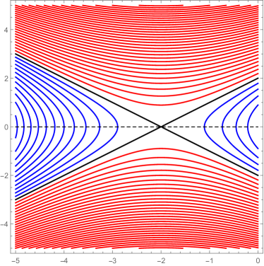
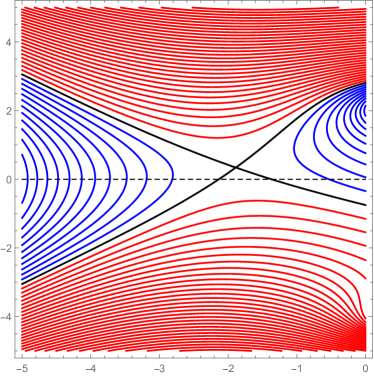
Figure 3. Level lines of the function $t\mapsto\operatorname{Re}S(t;z)$ in the left half-plane $\{\operatorname{Re}t\leq 0\}$. Left panel: $z=0$. Right panel: $z\neq 0$. In both cases, $\sigma=2$. The level set passing through the saddle point is shown in black. Level lines where the function takes smaller (respectively, larger) values than at the saddle point are shown in blue (respectively, red).

We are now going to apply the saddle-point method [59, § 45.4, p. 423] to the integral $\int_{-\infty}^{0}{\rm e}^{nS(t;z)}\textup{d}t$. To this end, we shall replace the initial contour of integration by a contour $\gamma$ (depending on $z$ and $\sigma^{2}$) with the following properties. The contour $\gamma$ starts at $-\infty$, ends at $0$, and stays in the left half-plane $\operatorname{Re}t\leq 0$. Furthermore, $\gamma$ passes through the saddle point $t_{0}=t_{0}(z)=t_{0}(z;\sigma^{2})$, and satisfies $\operatorname{Re}S(t;z)<\operatorname{Re}S(t_{0}(z);z)$ for all $t\in\gamma\backslash\{t_{0}(z)\}$. Finally, in the neighborhood of the point $t_{0}(z)$, the contour is required to pass through both sectors in which $\operatorname{Re}S(t;z)<\operatorname{Re}S(t_{0}(z);z)$. We shall prove the existence of such a contour provided $|z|$ is sufficiently small (even though we conjecture that it exists for all $z\in\mathbb{D}$). Let $\partial_{1}S$ and $\partial_{2}S$ denote the partial derivatives of $S(\cdot,\cdot)$ in the first/second argument. First of all, for $z=0$, the function $S(t;0)=-\frac{1}{2}(\frac{t}{\sigma}+\frac{\sigma}{2})^{2}$ attains its strict maximum on $(-\infty,0]$ at $t_{0}(0)=-\frac{1}{2}\sigma^{2}$. This critical point is simple meaning that $(\partial_{1}^{2}S)(-\frac{1}{2}\sigma^{2};0)<0$. It follows that the negative half-line $(-\infty,0]$ satisfies the conditions listed above; see the left panel of Figure 3. Observe also that in a small disk $D$ centered at $-\frac{1}{2}\sigma^{2}$, the set where $\operatorname{Re}S(t;0)<\operatorname{Re}S(-\frac{1}{2}\sigma^{2};0)$ consists of two sectors whose boundaries are straight lines crossing $D$ at four points $A_{1},A_{2},A_{3},A_{4}$. After a small perturbation of $z$, we still have a critical point at $t_{0}(z)$ which is close to $t_{0}(0)$ and simple, by analyticity of $t_{0}(z)$ and $S$; see Lemma 3.6. It follows that, in the disk $D$, the set where $\operatorname{Re}S(t;z)<\operatorname{Re}S(t_{0}(z);z)$ still consists of two sectors; see the right panel of Figure 3. The four points where the boundaries of these sectors cross $D$ are close to the points $A_{1},A_{2},A_{3},A_{4}$, again by analyticity. It follows that the saddle-point contour $\gamma$ satisfying the above condition exists (and can be obtained by perturbing the segment of the real line contained in $D$). Applying the saddle-point asymptotics [59, § 45.4, p. 423], we have

$$\int_{-\infty}^{0}{\rm e}^{nS(t;z)}\textup{d}t\sim\sqrt{-\frac{2\pi}{n(\partial_{1}^{2}S)(t_{0}(z);z)}}{\rm e}^{nS(t_{0}(z);z)},\qquad\text{ as }n\to\infty.$$ (3.11)

This holds pointwise in $z$ provided $|z|$ is sufficiently small (the uniformity in $z$ will be addressed later). It follows from (3.8) and (3.10) that for $z=-{\rm e}^{{\rm{i}}\theta}\neq 0$ we have

$$S(t_{0}(z);z)=\log(1-z{\rm e}^{t_{0}(z)})-\frac{1}{2}\left(\frac{t_{0}(z)}{\sigma}+\frac{\sigma}{2}\right)^{2}=\log(1+{\rm e}^{2{\rm{i}}\zeta_{\sigma^{2}/4}(\theta/2)})-\frac{\sigma^{2}}{2(1+{\rm e}^{-2{\rm{i}}\zeta_{\sigma^{2}/4}(\theta/2)})^{2}}.$$ (3.12)

Note that for $z=0$ we have $S(t_{0}(0);0)=0$. For future use let us note the identity

$$\frac{\textup{d}}{\textup{d}z}S(t_{0}(z);z) =(\partial_{1}S)(t_{0}(z);z)\partial_{z}t_{0}(z)+(\partial_{2}S)(t_{0}(z);z)=(\partial_{2}S)(t_{0}(z);z)$$

$$=-\frac{{\rm e}^{t_{0}(z)}}{1-z{\rm e}^{t_{0}(z)}}=\frac{1}{z}\left(\frac{1}{2}+\frac{t_{0}(z)}{\sigma^{2}}\right)$$

$$=-{\rm e}^{-{\rm{i}}\theta}\left(\frac{{\rm{i}}}{2}\tan\zeta_{\sigma^{2}/4}(\theta/2)+\frac{1}{2}\right)=\frac{-{\rm e}^{-{\rm{i}}\theta}}{1+{\rm e}^{-2{\rm{i}}\zeta_{\sigma^{2}/4}(\theta/2)}},$$ (3.13)

where we used that $(\partial_{1}S)(t_{0}(z);z)=0$ since $t=t_{0}(z)$ solves the saddle-point equation (3.9).

Contribution of the positive half-axis is negligible. We claim that if $r=r(\sigma^{2})>0$ is sufficiently small, then uniformly over the disk $|z|\leq r$ it holds that

$$\int_{0}^{\infty}(1-z{\rm e}^{t})^{n}{\rm e}^{-\frac{n}{2}\left(\frac{t}{\sigma}+\frac{\sigma}{2}\right)^{2}}\textup{d}t=O({\rm e}^{-\frac{1}{16}\sigma^{2}n}),\qquad\text{ as }n\to\infty.$$ (3.14)

If $0\leq t\leq\sigma^{2}$, then by choosing a sufficiently small $r>0$ we can achieve that $|1-z{\rm e}^{t}|\leq 1+|z|{\rm e}^{t}<{\rm e}^{\frac{1}{16}\sigma^{2}}$ for all $|z|\leq r$ and hence, for all $n\in\mathbb{N}$,

$$\Big{|}(1-z{\rm e}^{t})^{n}{\rm e}^{-\frac{n}{2}\left(\frac{t}{\sigma}+\frac{\sigma}{2}\right)^{2}}\Big{|}\leq{\rm e}^{\frac{1}{16}\sigma^{2}n}{\rm e}^{-\frac{1}{8}\sigma^{2}n}={\rm e}^{-\frac{1}{16}\sigma^{2}n}.$$

It follows that

$$\int_{0}^{\sigma^{2}}(1-z{\rm e}^{t})^{n}{\rm e}^{-\frac{n}{2}\left(\frac{t}{\sigma}+\frac{\sigma}{2}\right)^{2}}\textup{d}t=O(-{\rm e}^{\frac{1}{16}\sigma^{2}n}),\qquad\text{ as }n\to\infty.$$ (3.15)

For $t\geq\sigma^{2}$ we argue as follows. Since $1\leq{\rm e}^{t}$ for all $t\geq 0$, we have $|1-z{\rm e}^{t}|\leq 1+|z|{\rm e}^{t}\leq{\rm e}^{t}(1+r)$ provided $|z|\leq r$. It follows that

$$\Big{|}\int_{\sigma^{2}}^{\infty}(1-z{\rm e}^{t})^{n}{\rm e}^{-\frac{n}{2}\left(\frac{t}{\sigma}+\frac{\sigma}{2}\right)^{2}}\textup{d}t\Big{|}\leq(1+r)^{n}\int_{\sigma^{2}}^{\infty}{\rm e}^{-\frac{n}{2}\left(\frac{t}{\sigma}-\frac{\sigma}{2}\right)^{2}}\textup{d}t=(1+r)^{n}{\rm e}^{-\frac{1}{8}\sigma^{2}(n-1)}\int_{\sigma^{2}}^{\infty}{\rm e}^{-\frac{1}{2}\left(\frac{t}{\sigma}-\frac{\sigma}{2}\right)^{2}}\textup{d}t$$

since $\frac{1}{2}(\frac{t}{\sigma}-\frac{\sigma}{2})^{2}\geq\frac{1}{8}\sigma^{2}$ for $t\geq\sigma^{2}$. Note that the integral on the right-hand side converges. Also, if $r>0$ is sufficiently small, then $1+r\leq{\rm e}^{\frac{1}{16}\sigma^{2}}$ and it follows that

$$\int_{\sigma^{2}}^{\infty}(1-z{\rm e}^{t})^{n}{\rm e}^{-\frac{n}{2}\left(\frac{t}{\sigma}+\frac{\sigma}{2}\right)^{2}}\textup{d}t=O({\rm e}^{-\frac{1}{16}\sigma^{2}n}),\qquad\text{ as }n\to\infty.$$ (3.16)

Combining (3.15) and (3.16) yields (3.14), thus completing the proof that the contribution of the positive half-line is negligible.

Exact asymptotics of $H_{n}$. It follows from (3.11) and (3.14), together with the fact that $S(t_{0}(z);z)$ converges to $0$ as $z\to 0$, that, for sufficiently small $|z|$, the contribution of the positive half-axis is negligible in the sense that

$$\int_{-\infty}^{\infty}{\rm e}^{nS(t;z)}\textup{d}t\sim\sqrt{-\frac{2\pi}{n(\partial_{1}^{2}S)(t_{0}(z);z)}}{\rm e}^{nS(t_{0}(z);z)},\qquad\text{ as }n\to\infty.$$

In view of Lemma 3.4, we can write this as

$$\frac{H_{n}(z;\sigma^{2}/n)}{(-1)^{n}}\sim\sqrt{-\frac{1}{\sigma^{2}(\partial_{1}^{2}S)(t_{0}(z);z)}}{\rm e}^{nS(t_{0}(z);z)}\qquad\text{ as }n\to\infty.$$ (3.17)

This holds pointwise for every $|z|\leq r$ provided that $r>0$ is sufficiently small. Although we shall non need this fact, let us mention that after some work it is possible to verify that

$$(\partial_{1}^{2}S)(t_{0};z)=\frac{z^{-1}{\rm e}^{-t_{0}(z)}}{(1-z^{-1}{\rm e}^{-t_{0}(z)})^{2}}-\frac{1}{\sigma^{2}}=-\frac{1}{4\cos^{2}\zeta_{\sigma^{2}/4}(\theta/2)}-\frac{1}{\sigma^{2}}.$$ (3.18)

Proof of the uniform convergence. Now we would like to take the logarithm of both sides of (3.17). Observe that the left-hand side cannot become zero for $z\in\mathbb{D}$ by Lemma 2.1. Trivially, the same conclusion holds for the right-hand side. Therefore, applying the function $w\mapsto\log|w|$ to both sides of (3.17) and dividing by $n$ we get

$$\lim_{n\to\infty}\frac{1}{n}\log\left|\frac{H_{n}(z;\sigma^{2}/n)}{(-1)^{n}}\right|=\operatorname{Re}S(t_{0}(z);z).$$ (3.19)

This holds pointwise in $z$ provided $|z|\leq r$ with $r>0$ sufficiently small. Note that we did not apply the function $w\mapsto\log w$ to avoid difficulties with the choice of the branch. Now, our aim is to prove that

$$\lim_{n\to\infty}\frac{1}{n}\log\frac{H_{n}(z;\sigma^{2}/n)}{(-1)^{n}}=S(t_{0}(z);z)$$ (3.20)

locally uniformly in $|z|<r$ and with the same convention for the logarithm as in Proposition 3.5. To this end, we shall use the following lemma which strengthens [41, Lemma 3.8].

Lemma 3.7.

Let $h_{1}(z),h_{2}(z),\ldots$ be a sequence of holomorphic functions defined on some domain $\mathcal{D}\subset\mathbb{C}$. If $\operatorname{Re}h_{n}(z)\to 0$ pointwise on $\mathcal{D}$ and the sequence $(\operatorname{Re}h_{n}(z))_{n\in\mathbb{N}}$ is locally uniformly bounded from above on $\mathcal{D}$, then $h_{n}^{\prime}(z)\to 0$ locally uniformly on $\mathcal{D}$.

Remark 3.8.

If, additionally, $h_{n}(y_{0})\to 0$ for some $y_{0}\in\mathcal{D}$, then, integrating, we conclude that $h_{n}(z)\to 0$ locally uniformly on $\mathcal{D}$.

Proof of Lemma 3.7..

Consider some closed disk $B$ contained in $\mathcal{D}$ and centered at $z_{0}\in\mathcal{D}$. We know that $\operatorname{Re}h_{n}(z)\leq C$, for all $n\in\mathbb{N}$ and $z\in B$. Also, we know that $\operatorname{Re}f_{n}(z_{0})$ converges (and hence is bounded below). By Harnack’s inequality applied to the non-negative harmonic functions $C-\operatorname{Re}h_{n}(z)$ it follows that $C-\operatorname{Re}h_{n}(z)$ is uniformly bounded from above on $B$. We conclude that the sequence $(\operatorname{Re}h_{n}(z))_{n\in\mathbb{N}}$ is locally uniformly bounded, both from above and from below.

Take some $z_{0}\in\mathcal{D}$ and let $B_{r}(z_{0})\subset\mathcal{D}$ be a closed disk of radius $r$ centered at $z_{0}$ and contained in $\mathcal{D}$. It is known (see, e.g., the proof of Lemma 3.8 in [41]) that for all $z$ in the interior of $B_{r}(z_{0})$, we have

$$h_{n}^{\prime}(z)=\frac{1}{\pi{\rm{i}}}\oint_{|w-z_{0}|=r}\frac{\operatorname{Re}h_{n}(w)}{(w-z)^{2}}\textup{d}w,$$ (3.21)

where the integration contour is the boundary of $B_{r}(z_{0})$, oriented counter-clockwise. Having (3.21) at our disposal, we claim that $h_{n}^{\prime}(z)\to 0$ uniformly over $z\in B_{r/2}(z_{0})$. Recall that $\operatorname{Re}h_{n}(w)/(w-z)^{2}\to 0$ pointwise on $\mathcal{D}$. Additionally, we know that $|\operatorname{Re}h_{n}(w)/(w-z)^{2}|<C_{1}$ for all $n\in\mathbb{N}$, $z\in B_{r/2}(z_{0})$ and $w\in\partial B_{r}(z_{0})$. While the pointwise convergence $h_{n}^{\prime}(z)\to 0$ follows from (3.21) together with the dominated convergence theorem, an additional argument is needed to prove uniformity. Let $\varepsilon>0$ be given. By Egorov’s theorem, $\operatorname{Re}h_{n}(w)\to 0$ uniformly provided $w$ stays outside some subset $A_{\varepsilon}\subset\partial B_{r}(z_{0})$ of one-dimensional Lebesgue measure at most $\varepsilon$. Hence, $\operatorname{Re}h_{n}(w)/(w-z)^{2}\to 0$ uniformly in $z\in B_{r/2}(z_{0})$ and $w\in\partial B_{r}(z_{0})\backslash A_{\varepsilon}$. Thus, the integrals in (3.21) taken over the complement of $A_{\varepsilon}$ converge to $0$ uniformly. The integrals over $A_{\varepsilon}$ can be bounded by $C_{1}\varepsilon$, and the claim follows. ∎

We apply Lemma 3.7 with $h_{n}(z):=\frac{1}{n}\log\frac{H_{n}(z;\sigma^{2}/n)}{(-1)^{n}}-S(t_{0}(z);z)$. These functions are analytic on $\{|z|<r\}$ and we have $h_{n}(0)=0$ as well as $\operatorname{Re}h_{n}(z)\to 0$ pointwise, by (3.19). Observe that the functions $(\operatorname{Re}h_{n}(z))_{n\in\mathbb{N}}$ are locally uniformly bounded from above since by (1.5) and the triangle inequality,

$$\frac{1}{n}\log\left|\frac{H_{n}(z;\sigma^{2}/n)}{(-1)^{n}}\right|\leq\frac{1}{n}\log\left(\sum_{j=0}^{n}\binom{n}{j}|z|^{j}\right)\leq\log(1+|z|),\qquad z\in\mathbb{C}.$$

Lemma 3.7 (together with Remark 3.8) yields (3.20). Taking into account (3.12), this proves Proposition 3.5. Since a locally uniform convergence of analytic functions can be differentiated, we infer that

$$\lim_{n\to\infty}\frac{1}{n}\cdot\frac{H_{n}^{\prime}(z;\sigma^{2}/n)}{H_{n}(z;\sigma^{2}/n)} =\frac{\textup{d}}{\textup{d}z}S(t_{0}(z);z)=\frac{-{\rm e}^{-{\rm{i}}\theta}}{1+{\rm e}^{-2{\rm{i}}\zeta_{\sigma^{2}/4}(\theta/2)}}=-{\rm e}^{-{\rm{i}}\theta}\left(\frac{{\rm{i}}}{2}\tan\zeta_{\sigma^{2}/4}(\theta/2)+\frac{1}{2}\right);$$

see (3.13). The proof of Proposition 3.1 is complete. $\Box$

References

- Akemann et al. [2021] G. Akemann, F. Götze, and T. Neuschel. Characteristic polynomials of products of non-Hermitian Wigner matrices: finite- results and Lyapunov universality. Electron. Commun. Probab., 26:Paper No. 30, 13, 2021. doi: 10.1214/21-ecp398. URL https://doi.org/10.1214/21-ecp398.
- Aleman et al. [2004] A. Aleman, D. Beliaev, and H. Hedenmalm. Real zero polynomials and Pólya-Schur type theorems. J. Anal. Math., 94:49–60, 2004. doi: 10.1007/BF02789041. URL https://doi.org/10.1007/BF02789041.
- Anderson et al. [2010] G. W. Anderson, A. Guionnet, and O. Zeitouni. An introduction to random matrices, volume 118 of Cambridge Studies in Advanced Mathematics. Cambridge University Press, Cambridge, 2010.
- Andraus et al. [2012] S. Andraus, M. Katori, and S. Miyashita. Interacting particles on the line and Dunkl intertwining operator of type A: application to the freezing regime. J. of Physics A: Math. and Theoret., 45(39):395201, sep 2012. doi: 10.1088/1751-8113/45/39/395201. URL https://doi.org/10.1088/1751-8113/45/39/395201.
- Aomoto [1987] K. Aomoto. Jacobi polynomials associated with Selberg integrals. SIAM J. Math. Anal., 18(2):545–549, 1987. doi: 10.1137/0518042. URL https://doi.org/10.1137/0518042.
- Arizmendi and Perales [2018] O. Arizmendi and D. Perales. Cumulants for finite free convolution. J. Combin. Theory Ser. A, 155:244–266, 2018. doi: 10.1016/j.jcta.2017.11.012. URL https://doi.org/10.1016/j.jcta.2017.11.012.
- Arizmendi et al. [2021] O. Arizmendi, J. Garza-Vargas, and D. Perales. Finite free cumulants: Multiplicative convolutions, genus expansion and infinitesimal distributions. Preprint at http://arxiv.org/abs/2108.08489, 2021.
- Benz [1934] E. Benz. Über lineare, verschiebungstreue Funktionaloperationen und die Nullstellen ganzer Funktionen. Comment. Math. Helv., 7(1):243–289, 1934. doi: 10.1007/BF01292721. URL https://doi.org/10.1007/BF01292721.
- Bercovici and Voiculescu [1992] H. Bercovici and D. Voiculescu. Lévy-Hinčin type theorems for multiplicative and additive free convolution. Pacific J. Math., 153(2), 1992. URL http://projecteuclid.org/euclid.pjm/1102635830.
- [10] P. Biane. Free Brownian motion, free stochastic calculus and random matrices. In Free probability theory (Waterloo, ON, 1995), volume 12 of Fields Inst. Commun., pages 1–19. Amer. Math. Soc., Providence, RI.
- Biane [1997] P. Biane. Segal-Bargmann transform, functional calculus on matrix spaces and the theory of semi-circular and circular systems. J. Funct. Anal., 144(1):232–286, 1997. doi: 10.1006/jfan.1996.2990. URL https://doi.org/10.1006/jfan.1996.2990.
- Biane [2009] P. Biane. Matrix valued Brownian motion and a paper by Pólya. In Séminaire de Probabilités XLII, volume 1979 of Lecture Notes in Math., pages 171–185. Springer, Berlin, 2009. doi: 10.1007/978-3-642-01763-6“˙7. URL https://doi.org/10.1007/978-3-642-01763-6_7.
- Billingsley [1968] P. Billingsley. Convergence of probability measures. John Wiley & Sons, Inc., New York-London-Sydney, 1968.
- Bøgvad et al. [2021] R. Bøgvad, C. Hägg, and B. Shapiro. Rodrigues’ descendants of a polynomial and Boutroux curves. Preprint at http://arxiv.org/abs/2107.05710, 2021.
- Brézin and Hikami [2000] E. Brézin and S. Hikami. Characteristic polynomials of random matrices. Comm. Math. Phys., 214(1):111–135, 2000. doi: 10.1007/s002200000256. URL https://doi.org/10.1007/s002200000256.
- Cabanal Duvillard and Guionnet [2001] T. Cabanal Duvillard and A. Guionnet. Large deviations upper bounds for the laws of matrix-valued processes and non-communicative entropies. Ann. Probab., 29(3):1205–1261, 2001. doi: 10.1214/aop/1015345602. URL https://doi.org/10.1214/aop/1015345602.
- Cébron [2016] G. Cébron. Matricial model for the free multiplicative convolution. Ann. Probab., 44(4):2427–2478, 2016. doi: 10.1214/15-AOP1024. URL https://doi.org/10.1214/15-AOP1024.
- Cépa and Lépingle [2001] E. Cépa and D. Lépingle. Brownian particles with electrostatic repulsion on the circle: Dyson’s model for unitary random matrices revisited. ESAIM Probab. Statist., 5:203–224, 2001. doi: 10.1051/ps:2001109. URL https://doi.org/10.1051/ps:2001109.
- Deger and Flindt [2020] A. Deger and C. Flindt. Lee-Yang theory of the Curie-Weiss model and its rare fluctuations. Phys. Rev. Research, 2:033009, Jul 2020. doi: 10.1103/PhysRevResearch.2.033009. URL https://link.aps.org/doi/10.1103/PhysRevResearch.2.033009.
- Deger et al. [2020] A. Deger, F. Brange, and C. Flindt. Lee-Yang theory, high cumulants, and large-deviation statistics of the magnetization in the Ising model. Phys. Rev. B, 102:174418, Nov 2020. doi: 10.1103/PhysRevB.102.174418. URL https://link.aps.org/doi/10.1103/PhysRevB.102.174418.
- Diaconis and Gamburd [2004/06] P. Diaconis and A. Gamburd. Random matrices, magic squares and matching polynomials. Electron. J. Combin., 11(2):Research Paper 2, 26, 2004/06. URL http://www.combinatorics.org/Volume_11/Abstracts/v11i2r2.html.
- Dumitriu and Edelman [2002] I. Dumitriu and A. Edelman. Matrix models for beta ensembles. J. Math. Phys., 43(11):5830–5847, 2002. doi: 10.1063/1.1507823. URL https://doi.org/10.1063/1.1507823.
- Dumitriu and Edelman [2005] I. Dumitriu and A. Edelman. Eigenvalues of Hermite and Laguerre ensembles: large beta asymptotics. Ann. Inst. H. Poincaré Probab. Statist., 41(6):1083–1099, 2005. ISSN 0246-0203. doi: 10.1016/j.anihpb.2004.11.002. URL https://doi.org/10.1016/j.anihpb.2004.11.002.
- Dyson [1962] F. J. Dyson. A Brownian-motion model for the eigenvalues of a random matrix. J. Mathematical Phys., 3:1191–1198, 1962. doi: 10.1063/1.1703862. URL https://doi.org/10.1063/1.1703862.
- Edelman [1989] A. Edelman. Eigenvalues and condition numbers of random matrices. https://dspace.mit.edu/handle/1721.1/14322, 1989. PhD Thesis, Massachusetts Institute of Technology.
- Ellis [2006] R. S. Ellis. Entropy, large deviations, and statistical mechanics. Classics in Mathematics. Springer-Verlag, Berlin, 2006. doi: 10.1007/3-540-29060-5. URL https://doi.org/10.1007/3-540-29060-5. Reprint of the 1985 original.
- Ellis and Newman [1978a] R. S. Ellis and C. M. Newman. Limit theorems for sums of dependent random variables occurring in statistical mechanics. Z. Wahrsch. Verw. Gebiete, 44(2):117–139, 1978a. doi: 10.1007/BF00533049. URL https://doi.org/10.1007/BF00533049.
- Ellis and Newman [1978b] R. S. Ellis and C. M. Newman. The statistics of Curie-Weiss models. J. Statist. Phys., 19(2):149–161, 1978b. doi: 10.1007/BF01012508. URL https://doi.org/10.1007/BF01012508.
- Ellis et al. [1980] R. S. Ellis, C. M. Newman, and J. S. Rosen. Limit theorems for sums of dependent random variables occurring in statistical mechanics. II. Conditioning, multiple phases, and metastability. Z. Wahrsch. Verw. Gebiete, 51(2):153–169, 1980. doi: 10.1007/BF00536186. URL https://doi.org/10.1007/BF00536186.
- Fisher [1965] M. E. Fisher. The nature of critical points. volume 7c of Lecture Notes in Theoretical Physics, pages 1–159. Boulder: University of Colorado Press, 1965.
- Forrester and Gamburd [2006] P. J. Forrester and A. Gamburd. Counting formulas associated with some random matrix averages. J. Combin. Theory Ser. A, 113(6):934–951, 2006. doi: 10.1016/j.jcta.2005.09.001. URL https://doi.org/10.1016/j.jcta.2005.09.001.
- Friedli and Velenik [2018] S. Friedli and Y. Velenik. Statistical mechanics of lattice systems. Cambridge University Press, Cambridge, 2018. A concrete mathematical introduction.
- Galligo [2022] A. Galligo. Modeling complex root motion of real random polynomials under differentiation. Preprint at https://hal.archives-ouvertes.fr/hal-03577445/, 2022.
- Gawronski [1987] W. Gawronski. On the asymptotic distribution of the zeros of Hermite, Laguerre, and Jonquière polynomials. J. Approx. Theory, 50(3):214–231, 1987. ISSN 0021-9045. doi: 10.1016/0021-9045(87)90020-7. URL https://doi.org/10.1016/0021-9045(87)90020-7.
- Glasser et al. [1986] M. L. Glasser, V. Privman, and L. S. Schulman. Complex temperature plane zeros in the mean-field approximation. J. Statist. Phys., 45(3-4):451–457, 1986. doi: 10.1007/BF01021081. URL https://doi.org/10.1007/BF01021081.
- Gorin and Kleptsyn [2020] V. Gorin and V. Kleptsyn. Universal objects of the infinite beta random matrix theory. Preprint at http://arxiv.org/abs/2009.02006, 2020.
- Hall [2018] B. Hall. The eigenvalue process for Brownian motion in . Preprint at https://www3.nd.edu/~bhall/publications/documents/NonIntersecting.pdf, 2018.
- Hall and Ho [2022] B.C. Hall and C.-W. Ho. The heat flow conjecture for random matrices. Preprint at http://arxiv.org/abs/2202.09660, 2022.
- Hobson and Werner [1996] D. G. Hobson and W. Werner. Non-colliding Brownian motions on the circle. Bull. London Math. Soc., 28(6):643–650, 1996. doi: 10.1112/blms/28.6.643. URL https://doi.org/10.1112/blms/28.6.643.
- Hoskins and Kabluchko [2021] J. Hoskins and Z. Kabluchko. Dynamics of zeroes under repeated differentiation. Experimental Mathematics, 0(0):1–27, 2021. doi: 10.1080/10586458.2021.1980752. URL https://doi.org/10.1080/10586458.2021.1980752.
- Kabluchko [2021] Z. Kabluchko. Repeated differentiation and free unitary Poisson process. Preprint at http://arxiv.org/abs/2112.14729, 2021.
- Kemp [2017] T. Kemp. Heat kernel empirical laws on and . J. Theoret. Probab., 30(2):397–451, 2017. doi: 10.1007/s10959-015-0643-7. URL https://doi.org/10.1007/s10959-015-0643-7.
- Kiselev and Tan [2020] A. Kiselev and C. Tan. The flow of polynomial roots under differentiation. Preprint at http://arxiv.org/abs/2012.09080, 2020.
- Kornyik and Michaletzky [2016] M. Kornyik and G. Michaletzky. Wigner matrices, the moments of roots of Hermite polynomials and the semicircle law. J. Approx. Theory, 211:29–41, 2016. doi: 10.1016/j.jat.2016.07.006. URL https://doi.org/10.1016/j.jat.2016.07.006.
- Krasnytska et al. [2016] M. Krasnytska, B. Berche, Yu. Holovatch, and R Kenna. Partition function zeros for the Ising model on complete graphs and on annealed scale-free networks. Journal of Physics A: Mathematical and Theoretical, 49(13):135001, feb 2016. doi: 10.1088/1751-8113/49/13/135001. URL https://doi.org/10.1088/1751-8113/49/13/135001.
- Lee and Yang [1952] T. D. Lee and C. N. Yang. Statistical theory of equations of state and phase transitions. II. Lattice gas and Ising model. Phys. Rev. (2), 87:410–419, 1952.
- Lévy [2008] T. Lévy. Schur-Weyl duality and the heat kernel measure on the unitary group. Adv. Math., 218(2):537–575, 2008. doi: 10.1016/j.aim.2008.01.006. URL https://doi.org/10.1016/j.aim.2008.01.006.
- Marcus [2018] A. W. Marcus. Polynomial convolutions and (finite) free probability. Preprint at https://arxiv.org/abs/2108.07054, 2018.
- Marcus et al. [2022] A. W. Marcus, D. A. Spielman, and N. Srivastava. Finite free convolutions of polynomials. Probab. Theory Relat. Fields, 182(3-4):807–848, 2022. doi: https://doi.org/10.1007/s00440-021-01105-w.
- Méliot and Nikeghbali [2015] P.-L. Méliot and A. Nikeghbali. Mod-Gaussian convergence and its applications for models of statistical mechanics. In In memoriam Marc Yor—Séminaire de Probabilités XLVII, volume 2137 of Lecture Notes in Math., pages 369–425. Springer, Cham, 2015. doi: 10.1007/978-3-319-18585-9“˙17. URL https://doi.org/10.1007/978-3-319-18585-9_17.
- Mirabelli [2021] B. Mirabelli. Hermitian, Non-Hermitian and Multivariate Finite Free Probability. 2021. URL https://dataspace.princeton.edu/handle/88435/dsp019593tz21r. PhD Thesis, Princeton University.
- Nica and Speicher [2006] A. Nica and R. Speicher. Lectures on the combinatorics of free probability, volume 335 of London Mathematical Society Lecture Note Series. Cambridge University Press, Cambridge, 2006. doi: 10.1017/CBO9780511735127. URL https://doi.org/10.1017/CBO9780511735127.
- O’Rourke and Steinerberger [2021] S. O’Rourke and S. Steinerberger. A nonlocal transport equation modeling complex roots of polynomials under differentiation. Proc. Amer. Math. Soc., 149:1581–1592, 2021. URL https://doi.org/10.1090/proc/15314.
- Potters and Bouchaud [2021] M. Potters and J.-P. Bouchaud. A first course in random matrix theory: for physicists, engineers and data scientists. Cambridge: Cambridge University Press, 2021. doi: 10.1017/9781108768900.
- Revuz and Yor [1999] D. Revuz and M. Yor. Continuous martingales and Brownian motion, volume 293 of Grundlehren der mathematischen Wissenschaften. Springer-Verlag, Berlin, third edition, 1999. doi: 10.1007/978-3-662-06400-9. URL https://doi.org/10.1007/978-3-662-06400-9.
- Romik and Śniady [2015] D. Romik and P. Śniady. Jeu de taquin dynamics on infinite Young tableaux and second class particles. Ann. Probab., 43(2):682–737, 2015. doi: 10.1214/13-AOP873. URL https://doi.org/10.1214/13-AOP873.
- Ruelle [1969] D. Ruelle. Statistical mechanics: Rigorous results. W. A. Benjamin, Inc., New York-Amsterdam, 1969.
- Shamis and Zeitouni [2018] M. Shamis and O. Zeitouni. The Curie-Weiss model with complex temperature: phase transitions. J. Stat. Phys., 172(2):569–591, 2018. doi: 10.1007/s10955-017-1812-0. URL https://doi.org/10.1007/s10955-017-1812-0.
- Sidorov et al. [1985] Yu. V. Sidorov, M. V. Fedoryuk, and M. I. Shabunin. Lectures on the theory of functions of a complex variable. “Mir”, Moscow, 1985. Translated from the Russian by Eugene Yankovsky.
- Steinerberger [2019] S. Steinerberger. A nonlocal transport equation describing roots of polynomials under differentiation. Proc. Amer. Math. Soc., 147(11):4733–4744, 2019. doi: 10.1090/proc/14699. URL http://dx.doi.org/10.1090/PROC/14699.
- Steinerberger [2020] S. Steinerberger. Conservation laws for the density of roots of polynomials under differentiation. Preprint at http://arxiv.org/abs/2001.09967, 2020.
- Steinerberger [2021] S. Steinerberger. Free convolution powers via roots of polynomials. Experimental Mathematics, to appear, 2021. Preprint at http://arxiv.org/abs/2009.03869.
- Szegő [1975] G. Szegő. Orthogonal polynomials. American Mathematical Society Colloquium Publications, Vol. XXIII. American Mathematical Society, Providence, R.I., fourth edition, 1975.
- Tao [2017] T. Tao. Heat flow and zeroes of polynomials. https://terrytao.wordpress.com/2017/10/17/heat-flow-and-zeroes-of-polynomials/, 2017.
- Tao [2018] T. Tao. Heat flow and zeroes of polynomials II. https://terrytao.wordpress.com/2018/06/07/heat-flow-and-zeroes-of-polynomials-ii-zeroes-on-a-circle/, 2018.
- Ullman [1980] J. L. Ullman. Orthogonal polynomials associated with an infinite interval. Michigan Math. J., 27(3):353–363, 1980. URL http://projecteuclid.org/euclid.mmj/1029002408.
- Voiculescu [1985] D. Voiculescu. Symmetries of some reduced free product -algebras. In Operator algebras and their connections with topology and ergodic theory (Buşteni, 1983), volume 1132 of Lecture Notes in Math., pages 556–588. Springer, Berlin, 1985. doi: 10.1007/BFb0074909. URL https://doi.org/10.1007/BFb0074909.
- Voiculescu [1987] D. Voiculescu. Multiplication of certain noncommuting random variables. J. Operator Theory, 18(2):223–235, 1987. URL http://www.jstor.org/stable/24714784.
- Voiculescu et al. [1992] D. V. Voiculescu, K. J. Dykema, and A. Nica. Free random variables, volume 1 of CRM Monograph Series. American Mathematical Society, Providence, RI, 1992. doi: 10.1090/crmm/001. URL https://doi.org/10.1090/crmm/001.
- Voit and Woerner [2020] M. Voit and J. H. C. Woerner. Functional central limit theorems for multivariate Bessel processes in the freezing regime. Stochastic Analysis and Applications, 39(1):136–156, 2020. doi: 10.1080/07362994.2020.1786402. URL http://dx.doi.org/10.1080/07362994.2020.1786402.
- Voit and Woerner [2022] M. Voit and J. H. C. Woerner. Limit theorems for Bessel and Dunkl processes of large dimensions and free convolutions. Stoc. Proc. and their Appl., 143:207–253, 2022. doi: https://doi.org/10.1016/j.spa.2021.10.005. URL https://www.sciencedirect.com/science/article/pii/S030441492100168X.
- Yang and Lee [1952] C. N. Yang and T. D. Lee. Statistical theory of equations of state and phase transitions. I. Theory of condensation. Phys. Rev. (2), 87:404–409, 1952.
- Zhong [2014] P. Zhong. Free Brownian motion and free convolution semigroups: multiplicative case. Pacific J. Math., 269(1):219–256, 2014. doi: 10.2140/pjm.2014.269.219. URL https://doi.org/10.2140/pjm.2014.269.219.
- Zhong [2015] P. Zhong. On the free convolution with a free multiplicative analogue of the normal distribution. J. Theoret. Probab., 28(4):1354–1379, 2015. doi: 10.1007/s10959-014-0556-x. URL https://doi.org/10.1007/s10959-014-0556-x.