A Universal Triangulation for Flat Tori

Abstract

A result due to Burago and Zalgaller states that every orientable polyhedral surface, one that is obtained by gluing Euclidean polygons, has an isometric piecewise linear (PL) embedding into Euclidean space $\mathbb{E}^{3}$. A flat torus, resulting from the identification of the opposite sides of a Euclidean parallelogram, is a simple example of polyhedral surface. In a first part, we adapt the proof of Burago and Zalgaller, which is partially constructive, to produce PL isometric embeddings of flat tori. In practice, the resulting embeddings have a huge number of vertices, moreover distinct for every flat torus. In a second part, based on another construction of Zalgaller and on recent works by Arnoux et al., we exhibit a universal triangulation with 5974 triangles which can be embedded linearly on each triangle in order to realize the metric of any flat torus.

1 Introduction

A celebrated theorem of Nash [Nas54] completed by Kuiper [Kui55] implies that every smooth Riemannian orientable surface has a $C^{1}$ isometric embedding in the Euclidean 3-space $\mathbb{E}^{3}$. As a consequence one can represent and visualize faithfully in $\mathbb{E}^{3}$ the geometry of any abstract orientable Riemannian surface. An analogous result, due to Burago and Zalgaller [BZ95], states that every orientable polyhedral surface, obtained by abstractly gluing Euclidean polygons, has an isometric piecewise linear (PL) embedding in $\mathbb{E}^{3}$. In particular, this provides PL isometric embeddings for every flat torus, the result of the identification of the opposite sides of a Euclidean parallelogram. However, the proof of Burago and Zalgaller is partially constructive, relying on the subdivision of the polyhedral surface into an acute triangulation and on the Nash-Kuiper theorem itself, which is a priori far from constructive. The singular vertices of the polyhedral surface (where the angles at the incident polygons do not sum up to $2\pi$) moreover deserve special treatments with several constants that are rather hard to estimate. In the case of flat tori, all these difficulties can be circumvented. In particular, a flat torus has no singular vertex. Using a simple construction of acute triangulations together with the conformal embeddings of Hopf-Pinkall [Pin85, Ban88], we were able to compute PL isometric embeddings of various flat tori, including the square and the hexagonal tori.

In practice, the construction of Burago and Zalgaller, even including our simplifications for flat tori, produces PL embeddings with a huge number of vertices: more than 170,000 for the square torus and more than 7 millions for the hexagonal torus. Most importantly, the underlying triangulations of the resulting PL embeddings depends on the geometry (or modulus) of the flat tori and are pairwise non-isomorphic. Apart from the construction of Burago and Zalgaller, describing explicit PL embeddings of specific flat tori does not seem a simple task. As an illustrating example, it was only very recently that an explicit PL embedding of the square flat torus appeared in the literature [Qui20].

We say that a triangulation of the topological torus is universal if, for any flat torus, it admits a geometric realization in $\mathbb{E}^{3}$ that is isometric to this flat torus. It is not clear that such a universal triangulation should exist as the moduli space of flat tori is not compact. In particular, there is no reason why any of the triangulations obtained from the method of Burago and Zalgaller would be universal. Our main result is the rather surprising existence of a universal triangulation with the description of such a triangulation of reasonable size.

Theorem 1.

There exists an abstract triangulation $\cal T$ of the torus with 5974 triangles that admits for each flat torus (in the moduli space) an embedding in $\mathbb{E}^{3}$ which is linear on each triangle of $\cal T$, and which is isometric to this flat torus.

2 Background and definitions

Polyhedral surfaces

A polyhedral surface is a compact topological surface obtained from a finite collection of polygonal regions in the Euclidean plane by gluing their sides according to a partial oriented pairing. This pairing should be such that each side is paired at most once and two sides in a pair should have the same length. The pair orientation specifies one of the two isometries between its sides. Note that two sides of a same polygon may well be glued together. The resulting surface is closed, i.e., without boundary, when each side appears in one pair, i.e., when the pairing is complete. Since every polygon can be triangulated, one can replace the polygons by triangles in this definition. The collection of triangles together with their gluing determine a triangulation of the surface. This triangulation is simplicial when there is no loop edge or parallel edges, i.e., when no triangle side has its endpoints identified by the gluing and when any two triangle sides share a connected or empty subset after the gluing. By an abstract triangulation of a polyhedral surface, we mean a simplicial complex that is isomorphic to some triangulation of the polyhedral surface.

Polyhedral metric

The gluing of Euclidean polygons induces a length metric on the resulting polyhedral surface: the distance between any two points is the infimum of the lengths of the paths connecting the two points. Here, we consider paths that are finite concatenations of subpaths contained in a single polygon and the length of a path is the sum of the Euclidean length of these subpaths. There is an intrinsic definition of polyhedral surfaces that does not assume any specific decomposition into polygons. Formally, a polyhedral metric on a topological surface is a metric such that every point has a neighborhood isometric to a neighborhood of the apex of a Euclidean cone, where we ask that the isometry sends the considered point to the apex of the cone. In turn, a (2-dimensional) Euclidean cone is defined by coning from the origin a rectifiable simple (non self-intersecting) curve lying on the unit sphere in $\mathbb{E}^{3}$. The length of this curve is the total angle of the cone. A point whose conic neighborhood has total angle different from $2\pi$ is called a singular vertex. Note that in any triangulation of a polyhedral surface by Euclidean triangles the singular vertices must be vertices of the triangles.

Piecewise linear maps and isometries

Let $S$ be a polyhedral surface. A map $f:S\to\mathbb{E}^{3}$ is said piecewise linear (PL) if $S$ admits a triangulation such that the restriction of $f$ to any triangle is linear, i.e., it preserves barycentric coordinates. Once a triangulation of $S$ is given, the image of its vertices in $\mathbb{E}^{3}$ determines a unique linear map on this triangulation by extending linearly to the images of triangles.

$f$ is piecewise distance preserving if $S$ admits a triangulation such that the restriction of $f$ to any triangle is distance preserving, i.e., $|f(x)-f(y)|=d_{S}(x,y)$ for any $x,y$ in a same triangle. Here, $|\cdot|$ is the Euclidean norm and $d_{S}$ is the polyhedral metric on $S$. In particular, the piecewise distance preserving map $f$ must be length preserving: if $\gamma:[a,b]\to S$ is a rectifiable path, then $\gamma$ and its image $f\circ\gamma$ have the same length. The map $f$ is an embedding if it induces a homeomorphism onto its image $f(S)$ endowed with the restriction of the topology of $\mathbb{E}^{3}$. In that case, $f(S)$ is naturally equipped with a length metric induced by the Euclidean metric of $\mathbb{E}^{3}$ so that the length of a path in $f(S)$ is its Euclidean length as a path in $\mathbb{E}^{3}$.

A length preserving embedding is the same as an isometry between $S$ and $f(S)$, where each surface is endowed with its own length metric, respectively polyhedral and induced by the Euclidean metric. Thus, a piecewise distance preserving embedding is the same as a PL isometric embedding. A map $f:S\to\mathbb{E}^{3}$ is said contracting, or short, if there is a constant $C<1$ such that $|f(x)-f(y)|\leq Cd_{S}(x,y)$ for all $x,y\in S$.

Remark 1.

If $S$ is orientable, then it admits a short embedding into $\mathbb{E}^{3}$; simply embed $S$ into $\mathbb{E}^{3}$ as your favorite surface model with the same genus as $S$ and compose with a scaling of sufficiently small ratio to contract all distances. The model can be polyhedral or of any desired regularity.

Flat tori

A flat torus is a polyhedral surface obtained from a Euclidean parallelogram by pairing its opposite sides. We usually consider flat tori up to re-scaling since multiplying all the distances by the same constant does not modify the essential geometric properties of the torus. This amounts to consider that similar parallelograms lead to the same flat torus. If $(e_{1},e_{2})$ is the canonical basis of the Euclidean plane, we can thus assume that the two sides of the parallelogram are respectively $e_{1}$ and $\tau$ for some vector $\tau=\tau_{1}e_{1}+\tau_{i}e_{2}$, with $\tau_{i}>0$. Identifying the real plane with the complex line, we conclude that a flat torus is determined by its modulus $\tau=\tau_{1}+i\tau_{i}$.

Rather than gluing the sides of a parallelogram, one can equivalently obtained the same flat torus by quotienting the Euclidean plane $\mathbb{E}^{2}$ by the rank 2 lattice $\mathbb{Z}\tau+\mathbb{Z}e_{1}$ acting by translations. The same lattice is generated by the vectors $(a\tau+b,c\tau+d)$, where $\begin{pmatrix}a&b\\ c&d\end{pmatrix}\in\text{SL}_{2}(\mathbb{Z})$ is an integer matrix with determinant 1. After applying the adequate similarity, this lattice corresponds to the modulus $(a\tau+b)/(c\tau+d)$, where $\tau$ is again viewed as a complex number. In fact, the set of flat tori is in one-to-one correspondence with the quotient $\mathbb{H}^{2}/\text{SL}_{2}(\mathbb{Z})$, where $\mathbb{H}^{2}$ denotes the upper half-plane (the set of moduli) and $\text{SL}_{2}(\mathbb{Z})$ acts as above. Every flat torus has a modulus in the fundamental domain of this quotient as shown in Figure 1.

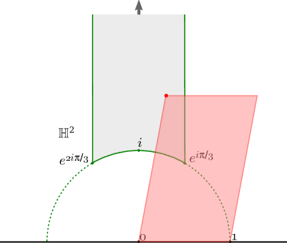
Figure 1: A point (in red) in a fundamental domain of the moduli space of tori (in light grey) with the corresponding parallelogram. Note that the boundary of the domain should be identified adequately to represent this moduli space faithfully, leading to a non-compact orbifold.

3 The construction of Burago and Zalgaller

We first recall the result of Burago and Zalgaller for embedded surfaces.

Theorem 2 (Burago and Zalgaller [BZ95]).

Every short $C^{2}$ embedding in $\mathbb{E}^{3}$ of a polyhedral surface can be approximated by a PL isometric embedding.

Here, the approximation by a PL isometric map means that for any $\varepsilon>0$ there is such a map moving the points of the short $C^{2}$-embedding by a distance less than $\varepsilon$. By Remark 1 this implies that every orientable polyhedral surface has an isometric PL embedding in 3-space. Before we give a sketch of the proof, we describe the basic construction of Burago and Zalgaller, which is a specialization of Theorem 2 to the case of a single triangle.

3.1 Embedding a triangle

We recall that a triangle is acute if its three internal angles are less than $\pi/2$. If $t$ is a triangle in $\mathbb{E}^{3}$ and $\vec{n}$ is a vector normal to $t$, then the prism above $t$ is the set $\{p+\lambda\vec{n}\mid p\in t,\lambda\geq 0\}$ and the three infinite faces of this prism are its walls.

Lemma 3 ([BZ95]).

Let $T=A_{1}A_{2}A_{3}$ and $t=a_{1}a_{2}a_{3}$ be (Euclidean) triangles in $\mathbb{E}^{3}$ such that

1. $T$ and $t$ are acute,

2. $|a_{i}a_{j}|<|A_{i}A_{j}|$ for $i,j=1,2,3;i\neq j$,

3. the distance of the circumcenter $\omega$ of $t$ to each side $a_{i}a_{j}$ is smaller than the distance of the circumcenter $\Omega$ of $T$ to the corresponding side $A_{i}A_{j}$.

Denote by $m_{ij}$ the point in the wall above $a_{i}a_{j}$ at equal distance from $a_{i}$ and $a_{j}$. Then, $T$ has a PL isometric embedding in the prism above $t$ (with respect to one of the two possible normal directions) with the boundary condition that each side $A_{i}A_{j}$ is sent to the broken line $a_{i}m_{ij}a_{j}$.

This Lemma (see Figure 2)

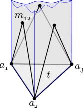
Figure 2: The prism above $t$.

easily implies that $T$ has a PL isometric embedding arbitrarily close to $t$. Indeed, by subdividing $T$ and $t$ uniformly as in Figure 3 we get similar triangles of smaller size to which we can individually apply Lemma 3. Thanks to the boundary condition in the lemma, the individual constructions fit together to form an isometric embedding of $T$. The constructions for the smaller triangles being homothetic to the construction for the original triangles, we get closer and closer to $t$ as we refine the uniform subdivisions.

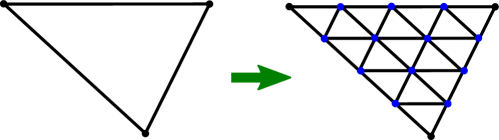
Figure 3: Uniform subdivision of a triangle. The vertices of the subdivision have barycentric coordinates $(i/n,j/n,k/n)$ for $i,j,k\in\mathbb{N}$ and $i+j+k=n$ for some fixed $n$.

The triangles $T$ and $t$ being acute, they contain their circumcenters $\Omega$ and $\omega$ in their interior. We let $\vec{n}$ be a unit vector normal to $t$ and we let $\omega^{\prime}$ be the point vertically above $\omega$ such that $|a_{1}\omega^{\prime}|=|A_{1}\Omega|$. Refer to Figure 4 for an illustration. Note that $\omega^{\prime}$ is well-defined since by the assumptions (ii) and (iii) the circumradius $|A_{1}\Omega|$ of $T$ is larger than the circumradius $|a_{1}\omega|$ of $t$. For completeness, we recall the proof of Lemma 3. Triangle $T$ is first subdivided into three subtriangles $\Omega A_{i}A_{j}$. The goal is to fold each $\Omega A_{i}A_{j}$ above $\omega a_{i}a_{j}$ with the boundary condition for $A_{i}A_{j}$ as in the lemma and so that the boundary edges $\Omega A_{i},\Omega A_{j}$ are sent respectively to the segments $\omega^{\prime}a_{i}$ and $\omega^{\prime}a_{j}$. To this end, we first fold $\Omega A_{1}A_{2}$ along its altitude from $\Omega$ and place the resulting two-winged shape above $t$ so that the side $A_{1}A_{2}$ is folded onto the broken line $a_{1}m_{12}a_{2}$.

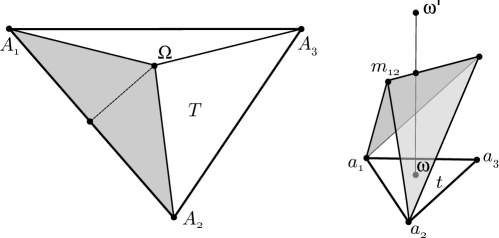
Figure 4: The subtriangle $\Omega A_{1}A_{2}$ is folded above $t$.

We next consider a plane $\Pi_{1}$ in the pencil generated by $a_{1}a_{2}$ to reflect the part of the two-winged shape lying to the right of that plane. See Figure 5.

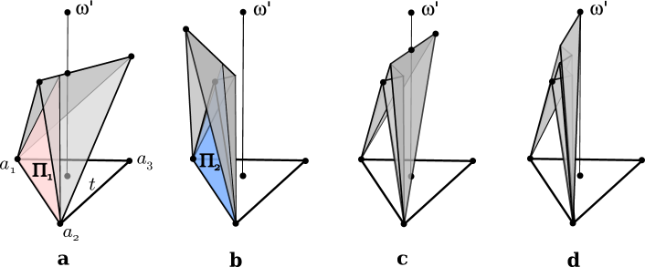
Figure 5: a, the reflection plane $\Pi_{1}$. b, after reflection in $\Pi_{1}$, and the plane $\Pi_{2}$. c, reflection in $\Pi_{2}$. d, after an even number of reflections the point $\Omega$ is sent to $\omega^{\prime}$.

Another plane $\Pi_{2}$ in the same pencil is then chosen to reflect part of the already reflected part. Choosing $\Pi_{1}$ and $\Pi_{2}$ appropriately, it is not hard to see that after an even number of such reflections the point $\Omega$ in $\Omega A_{1}A_{2}$ will be sent to $\omega^{\prime}$. We finally apply the same construction to the two other subtriangles $\Omega A_{2}A_{3}$ and $\Omega A_{3}A_{1}$ and paste them to form a folding of $T$ above $t$ as desired.

Note 4.

This folding of $T$ admits some flexibility. In particular, the boundary conditions can be modified so that each boundary wedge $a_{i}m_{ij}a_{j}$ is tilted around the axis $a_{i}a_{j}$. This modification is needed in order to paste the constructions above two adjacent triangles that are non coplanar as illustrated on Figure 6.

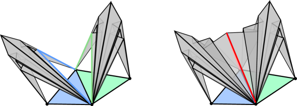
Figure 6: Pasting two foldings of large triangles sharing an edge above smaller triangles that are non coplanar.

3.2 Embedding arbitrary polyhedral surfaces

Denote by $f:S\to\mathbb{E}^{3}$ the short $C^{2}$ map in Theorem 2. Let $U$ be a union of small polygonal disks centered at each singular vertex of $S$. The strategy for the proof of Burago and Zalgaller is the following.

1. Compute an acute triangulation of $S\setminus U$, where each triangle is acute.

2. Compute an approximation $f_{1}$ of $f$ that is almost conformal on $S\setminus U$ and short over $S$. Here, almost conformal means that $f$ almost preserves angles, or more formally that its coefficient of quasi-conformality, or dilatation [FM12, Section 11.1.2], is close to one.

3. Refine the acute triangulation of $S\setminus U$ uniformly to obtain an acute triangulation $\cal T$ with small triangles. The meaning of small depends on the geometric properties of $f_{1}$ and on the flexibility in Note 4.

4. Replace $f_{1}$ by its PL approximation $F$ mapping linearly each triangle $T=A_{1}A_{2}A_{3}$ of $\cal T$ to the triangle $F(T):=f_{1}(A_{1})f_{1}(A_{2})f_{1}(A_{3})$ in $\mathbb{E}^{3}$.

5. Apply the construction in Section 3.1 to every pair $(T,F(T))$, using the tilted version in Note 4 in order to paste the constructions of adjacent triangles.

6. Fill the gaps corresponding to $U$ with specific constructions to deal with singularities as described in [BZ95], depending on whether the conical angle of a singularity is smaller or larger than $2\pi$.

We comment on the above steps, referring to the original paper [BZ95] for more details. Computing an acute triangulation as required in Step (a) is a non-trivial task. If $S$ is obtained from a gluing of Euclidean triangles it was shown how to compute an acute refinement [BZ60, Zam13] of reasonable size. Step (b) is the most challenging and relies on the Nash-Kuiper theorem [Nas54, Kui55]. The idea is to apply this theorem in order to approximate $f$ by an almost isometric map with respect to a metric homothetic to the metric on $S$, but slightly smaller. This provides the map $f_{1}$ that is at the same time short and almost conformal. This almost conformality combined with the uniform subdivision in Step (c) implies that any triangle $T$ of $\cal T$ is sent by the PL approximation $F$ of Step (d) to an almost similar triangle $F(T)$. Since $f_{1}$ and its PL approximation are short, this in turn implies that the pair $(T,F(T))$ satisfies Conditions (i),(ii) and (iii) in Lemma 3. Moreover, the fact that the triangles in $\cal T$ are small together with the smoothness of $f_{1}$ ensure that $F$ maps adjacent triangles to almost coplanar triangles. We can thus apply the basic construction of Lemma 3 and its tilted version as in Note 4 to perform Step (e). This eventually lead to a PL isometric embedding of $S\setminus U$. It remains to embed appropriately the neighborhood of the singular vertices as required by Step (f) to complete the PL isometric embedding of $S$.

4 Embedding flat tori

Step (b) in the proof of Burago and Zalgaller is highly non constructive, and to our knowledge no explicit PL isometric embedding of a closed surface according to their method was known up to date. It appears that the steps of their construction can be greatly simplified in the case of flat tori. Thanks to these simplifications we were able to visualize PL isometric embeddings of various flat tori in $\mathbb{E}^{3}$.

We first observe that there is no need for Step (f) since a flat torus has no singular vertex: the angles at the four corners of its defining parallelogram add up to $2\pi$, showing that the only vertex after the side gluing is non singular. In particular, one should set $U=\emptyset$ in all the steps.

4.1 Acute triangulation of flat tori

Itoha and Yuan [iIY09] have shown that every flat torus can be triangulated into at most 16 acute triangles. However, since we need a fine triangulation as in Step (c) with a good control on the acuteness, we use the following triangulation, which is conceptually simpler. Let $\tau$ be the modulus of the flat torus $\mathbb{T}_{\tau}:=\mathbb{E}^{2}/(\mathbb{Z}\tau+\mathbb{Z}e_{1})$ (we abusively identify the plane with the complex numbers). We consider the equilateral triangular lattice generated by $e^{i\pi/3}/n$ and $1/n$ for some positive integer $n$. This lattice comes with a regular triangulation ${\cal T}_{e}$ by equilateral triangles. Let $p_{a,b}=ae^{i\pi/3}/n+b/n$, with $a,b\in\mathbb{Z}$, be a point in this lattice that is closest to $\tau$. In particular, $|\tau-p_{a,b}|\leq(n\sqrt{3})^{-1}$. We deform ${\cal T}_{e}$ by a linear transformation $\ell$ defined by $1\mapsto 1$ and $p_{a,b}\mapsto\tau$. By the previous inequality and for $n$ large enough, $\ell$ is close to the identity. The triangles in $\ell({\cal T}_{e})$ are thus close to equilateral. Now, the lattice $\mathbb{Z}\tau+\mathbb{Z}e_{1}$ leaves $\ell({\cal T}_{e})$ invariant, so that $\ell({\cal T}_{e})/(\mathbb{Z}\tau+\mathbb{Z}e_{1})$ is a well defined triangulation of $\mathbb{T}_{\tau}$ by almost equilateral triangles. See Figure 7.

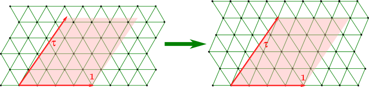
Figure 7: The equilateral triangular lattice (here with $n=4$) is deformed to fit the lattice of $\mathbb{T}_{\tau}$.

4.2 Conformal embedding of flat tori

Theorem 2 requires an initial short $C^{2}$ embedding, further approximated in Step (b) by an almost conformal map. In the case of flat tori we can directly provide a short conformal embedding.

The case of rectangular tori

For conciseness we identify $\mathbb{R}^{3}$ with $\mathbb{C}\times\mathbb{R}$. First observe that the standard embedding of the square torus as a torus of revolution, $f:\mathbb{T}_{1}\to\mathbb{E}^{3},(u,v)\mapsto\big{(}(R+r\cos(2\pi u))e^{i2\pi v},r\sin(2\pi u)\big{)}$, is never conformal as the ratio of the lengths of the partial derivatives is non-constant. The partial derivatives are nonetheless orthogonal and when the torus is rectangular, i.e., when $\tau=i\tau_{i}$ is pure imaginary, there are conformal maps of the form $f_{i\tau_{i}}:\mathbb{T}_{i\tau_{i}}\to\mathbb{E}^{3},(u,v)\mapsto f(\alpha(u),v/\tau_{i})$ for some $1$-periodic function $\alpha$. Indeed, when $\alpha$ satisfies the differential equation $\tau_{i}\alpha^{\prime}=\cos(2\pi\alpha)+\frac{R}{r}$, one easily check that the partial derivatives of $f_{i\tau_{i}}$ with respect to $u$ and $v$ have the same norm (and are orthogonal). This differential equation solves to

$$\alpha(u)=\frac{1}{\pi}\arctan\left(\sqrt{\frac{R+r}{R-r}}\tan\left(\frac{\sqrt{R^{2}-r^{2}}}{\tau_{i}r}\pi u\right)\right)\quad\text{with}\quad\frac{R}{r}=\sqrt{\tau_{i}^{2}k^{2}+1}$$

for some integer $k$. In practice, we have chosen $k=r=1$, leading to the conformal map:

$$f_{i\tau_{i}}(u,v)=\left(\left(\sqrt{\tau_{i}^{2}+1}+\cos\left(2\pi\alpha\left(u\right)\right)\right)e^{i2\pi v/\tau_{i}},\sin\left(2\pi\alpha\left(u\right)\right)\right)$$

with $\alpha(u)=\frac{1}{\pi}\arctan\left(\sqrt{\frac{\sqrt{\tau_{i}^{2}+1}+1}{\sqrt{\tau_{i}^{2}+1}-1}}\tan\left(\pi u\right)\right)$. It remains to compose $f_{i\tau_{i}}$ with a contracting homothety to get a short conformal embedding of $\mathbb{T}_{i\tau_{i}}$. See Figure 8 for an example.

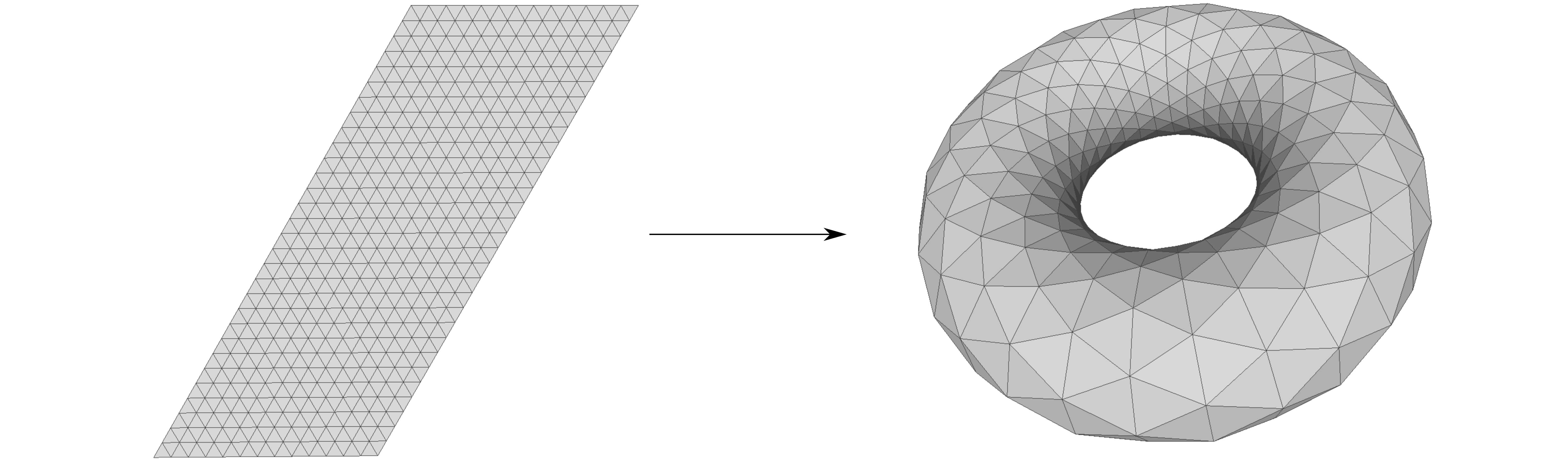
Figure 8: Left, the fundamental domain of the rectangular torus $\mathbb{T}_{2i}$ is chosen to be aligned with an almost equilateral tiling as in Section 4.1. Beware that the identification of the horizontal sides includes a non-integral translation. Right, PL approximation of the conformal embedding $f_{2i}$.

The general case

In order to embed non rectangular tori conformally we rely on the Hopf tori developed by Pinkall [Pin85]. These are based on the Hopf fibration

$$p:\mathbb{S}^{3}\to\mathbb{S}^{2},(x,y,z,t)\mapsto(2xz+2yt,2xt-2yz,x^{2}+y^{2}-z^{2}-t^{2}),$$

a standard projection of the 3-sphere $\mathbb{S}^{3}$ onto the 2-sphere $\mathbb{S}^{2}$ whose fibers (the sets $p^{-1}(s)$ for $s\in\mathbb{S}^{2}$) are circles. Pinkall proves that if $\gamma$ is a simple closed curve on $\mathbb{S}^{2}$, then $p^{-1}(\gamma)$ is a flat torus isometric to $\mathbb{T}_{\tau}$ with $\tau=(A+iL)/(4\pi)$, where $L$ is the length of $\gamma$ and $A$ is the oriented area delimited by $\gamma$ on $\mathbb{S}^{2}$, choosing the side of $\gamma$ so that $A\in[-2\pi,2\pi)$. Since this torus lies in $\mathbb{S}^{3}\subset\mathbb{E}^{4}$, it remains to apply a stereographic projection, say from the South pole $(0,0,0,-1)$, assuming it does not lie on the torus, to obtain a conformal embedding of $\mathbb{T}_{\tau}$ in $\mathbb{E}^{3}$. In coordinates: $(x,y,z,t)\mapsto(x,y,z)/(t+1)$.

Banchoff [Ban88] revisited Pinkall’s approach to give explicit parametrizations of the Hopf-Pinkall tori. On $\mathbb{S}^{2}$, Banchoff considers a curve of the form $\gamma_{\tau}(\theta)=(\sin\phi(\theta)e^{i\theta},\cos\phi(\theta))$ given in spherical coordinates, where the polar angle $0<\phi<\pi$ is a smooth function of the azimuthal angle $0\leq\theta\leq 2\pi$. He next defines $L(\theta)=\int_{0}^{\theta}|\gamma_{\tau}^{\prime}(t)|\text{d}t$ to be the length of the curve portion $\gamma_{\tau}([0,\theta])$ and $A(\theta)=\int_{0}^{\theta}(1-\cos\phi(t))\text{d}t$ the area on $\mathbb{S}^{2}$ swept by the arc of meridian linking the North Pole to the point on $\gamma_{\tau}$ up to $\theta$. The conformal embedding $f_{\tau}:\mathbb{T}_{\tau}\to\mathbb{E}^{3}$ is then given by $f_{\tau}=f\circ g^{-1}$ with

$$f:(\mathbb{R}/2\pi\mathbb{Z})^{2}\to\mathbb{E}^{3},(\theta,\psi)\mapsto\big{(}\sin\frac{\phi(\theta)}{2}e^{i(\theta+\psi)},\cos\psi\cos\frac{\phi(\theta)}{2}\big{)}/(1+\sin\psi\cos\frac{\phi(\theta)}{2}),\,\text{ and}$$

$$g:(\mathbb{R}/2\pi\mathbb{Z})^{2}\to\mathbb{T}_{-1/\tau}\sim\mathbb{T}_{\tau},(\theta,\psi)\mapsto(\frac{L(\theta)}{2},\frac{A(\theta)}{2}+\psi).$$

In other words,

$$f_{\tau}(u,v)=\big{(}\sin\frac{\phi(\theta)}{2}e^{i(\theta+u-A(\theta)/2)},\cos(u-A(\theta)/2)\cos\frac{\phi(\theta)}{2}\big{)}/(1+\sin(u-A(\theta)/2)\cos\frac{\phi(\theta)}{2}),$$

where $\theta$ satisfies $L(\theta)=2u$ and $(u,v)\in\mathbb{R}^{2}/(\mathbb{Z}2\pi i+\mathbb{Z}2\pi i\bar{\tau})$.

We have chosen $\phi$ of the form $\phi(\theta)=a+b\sin(n\theta)$ for $a<b$, $0\leq b<\pi-a$ and $n\in\mathbb{N}$. In order to represent the modulus $\tau=\tau_{1}+i\tau_{i}$, the parameters $a,b,n$ should satisfy $A(2\pi)=4\pi\tau_{1}$ and $L(2\pi)=4\pi\tau_{i}$, or equivalently:

$$J_{0}(b)\cos(a)=1-2\tau_{1}\quad\text{and}\quad\int_{0}^{2\pi}\sqrt{n^{2}b^{2}\cos^{2}(nt)+\sin^{2}(a+b\sin(nt))}\text{d}t=4\pi\tau_{i},$$

where $J_{0}(b)=\frac{1}{\pi}\int_{0}^{\pi}\cos(b\sin t)\text{d}t$ denotes the 0-th Bessel function of the first kind. The condition on the total area implies $0\leq\tau_{1}\leq 1$. Nevertheless, it is still possible to obtain a conformal embedding in the case of $\tau_{1}<0$ by first reflecting the torus along one of its boundary edge and applying a reflexion of the image torus in $\mathbb{E}^{3}$. We can thus cover the whole moduli space.

4.3 The final construction

We now have all the pieces to produce PL isometric embedding of flat tori. Given a modulus $\tau$, we first compute a quasi-equilateral triangulation of $\mathbb{T}_{\tau}$ as in Section 4.1. We then compute a PL approximation $F_{\tau}$ of the conformal map $f_{\tau}$ defined in Section 4.2 and finally apply the construction in Section 3.1 to every pair of triangles $(T,F_{\tau}(T))$. Figures 9 and 10 show some results.

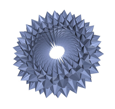
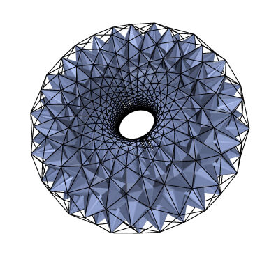
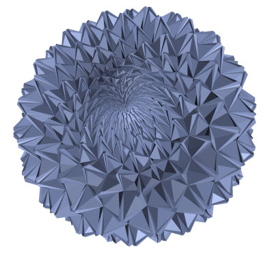
Figure 9: Left, PL isometric embedding of the square flat torus with 170,040 triangles. Middle, the mesh with black edges shows the PL approximation of the initial almost conformal embedding. Each of its triangles is replaced with a construction (in blue) as in Section 3.1 oriented toward the interior of the initial embedding. Right, The construction is oriented towards the outside, giving another isometric immersion of the square torus. (This last model has self-intersections. A finer triangulation should be used to avoid them.)

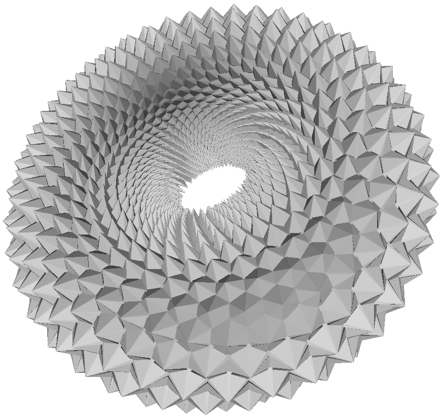
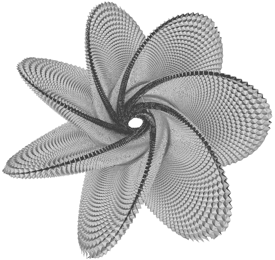
Figure 10: isometric immersion of $\mathbb{T}_{\tau}$ with, from left to right, $\tau=e^{i\pi/3},(1+i)/2,(1+3i)/2$. The left immersion is a hexagonal torus. While the subdivisions of the left and right tori already contain more than $7$ millions triangles, they present self-intersections. A finer triangulation should be used to get an embedding.

5 Universal triangulation

The construction of Burago and Zalgaller gives rise to triangulations with a huge number of triangles, moreover distinct for every flat torus. In order to get a unique abstract triangulation that admits linear embeddings in $\mathbb{E}^{3}$ isometric to any flat torus, we resort to a second construction by Zalgaller [Zal00] and to very recent work by Tsuboi [Tsu20] and Arnoux et al. [ALM21] for embedding flat tori.

5.1 Embedding long tori

Any flat torus can be obtained by identifying abstractly the top and bottom boundaries of a right circular cylinder. We obtain non-rectangular tori by shifting circularly the top boundary before identification. We can moreover cover all the torus moduli by varying the ratio between the height of the cylinder and the length of its boundaries. A torus is said long when this ratio is large. In [Zal00], Zalgaller proposes an origami style folding of long flat tori, much simpler that the general construction of [BZ95]. Here, we quantify how long should be a torus to allow for the Zalgaller folding, and we show that the long tori admit a universal triangulation.

Proposition 5.

There exists an abstract triangulation with 270 triangles, which admits linear embeddings isometric to every torus of modulus $\tau_{1}+i\tau_{i}$ with $\tau_{i}\geq 33$.

The proof reduces to a careful analysis of the construction of Zalgaller. Instead of a circular cylinder, Zalgaller starts with a polyhedral cylinder in $\mathbb{E}^{3}$, namely a prism with equilateral triangular basis, that he bents at several places to make the boundaries coincide, allowing their geometric identification. A twist is also applied before the bending so as to simulate a circular shift of the top boundary. In general, except for a twist of $2k\pi/3$, one boundary will be rotated with respect to the other after the twisting and bending, preventing their identification. Zalgaller then introduces a third modification that he calls a gasket in order to rotate a cross section of the prism without rotating the “material” of the prism. Intuitively, one should imagine a sleeve made of some non-elastic fabric, closed by two rigid triangles at the extremities. The right prism results from pulling tight on the triangles. Now, the effect of a gasket is to rotate one triangle around the axis of the prism, allowing the fabric to slide along the edges of this triangle.

How to bend a triangular prism

Consider a right prism $\cal P$ with equilateral triangular basis and an orthogonal cross section $CC^{\prime}D$. A bending at an angle $\varphi$ with cutting angle $\lambda$ along the rib $CC^{\prime}$ is obtained by (refer to Figure 11)

1. cutting two isosceles triangles $ACB$ and $AC^{\prime}B$ out of $\cal P$, where $A,B$ lie on the generatrix of the prism through $D$, and the angle at $C$ (and $C^{\prime}$) is $2\lambda$,

2. bending the cut prism at angle $0<\varphi<\pi$,

3. folding $ACB$ and $AC^{\prime}B$ appropriately to fit them back on the bended prism.

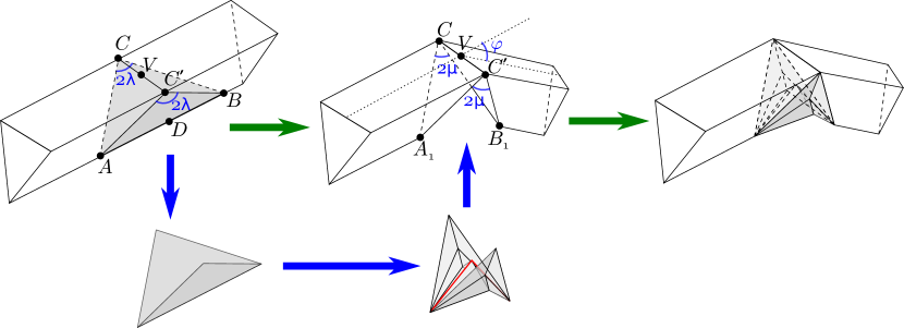
Figure 11: Bending of a prism.

Let $A_{1},B_{1}$ be the respective positions of points $A,B$ after bending and let $\angle{A_{1}CB_{1}}=2\mu$. In order for the construction not to overlap, one should have $\mu>0$, hence $\lambda$ should satisfy $\lambda_{0}(\varphi)<\lambda<\frac{\pi}{2}$ where $\lambda_{0}(\varphi)$ is the angle for which, after bending, the triangles $A_{1}CC^{\prime}$ and $B_{1}CC^{\prime}$ coincide. Looking at the right angled triangles $ADC$ and $ADV$, one easily computes

$$\lambda_{0}(\varphi)=\arctan(\frac{\sqrt{3}}{2}\tan\frac{\varphi}{2}).$$ (1)

Lemma 6.

For every $\varphi\in(0,\pi)$ and for every $\lambda\in(\lambda_{0}(\varphi),\pi/2)$, there is an embedded bending of $\cal P$ at angle $\varphi$ with cutting angle $\lambda$ introducing 12 triangles.

Proof.

We only have to check that $ACB$ and $AC^{\prime}B$ can be folded appropriately. The folding of $ACB$ (and of $AC^{\prime}B$) is very similar to the folding of a subtriangle as in Figure 5. We first fold $CAB$ along its altitude from $C$ to reduce the angle $(CA,CB)$ from $2\lambda$ to $2\mu$. The side $AB$ is mapped onto a broken line $A_{1}\tilde{D}B_{1}$ and the goal is to rotate this broken line so that it is contained in the “vertical” plane through $A_{1},B_{1},V$, where $V$ is the middle of $CC^{\prime}$. See Figure 11 and 12.

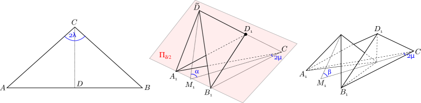
Figure 12: Folding of triangle $ACB$.

Denote by $\Pi_{0}$ the plane spanned by $A_{1},B_{1},C$. Also denote by $\Pi_{\theta}$ the plane, in the pencil of planes through $A_{1}B_{1}$, making an angle $\theta$ with $\Pi_{0}$. Let $\alpha,\beta$ be such that $\Pi_{\alpha}$ contains $\tilde{D}$ and $\Pi_{\beta}$ contains $V$. Because the triangles $C\tilde{D}M_{1}$ and $CVM_{1}$, where $M_{1}$ is the middle of $A_{1}B_{1}$, are right angled at $\tilde{D}$ and $V$, we easily deduce

$$\alpha=\arcsin\frac{\cos\lambda}{\cos\mu}\quad\text{and}\quad\beta=\arcsin\frac{\cos\lambda}{2\cos\mu}.$$

Set $\delta=\alpha-\beta$. The plane $\Pi_{\delta/2}$ cuts $C\tilde{D}$ in $D_{1}$. We first reflect across $\Pi_{\delta/2}$ the pieces of triangles $A_{1}CB_{1}$ and $A_{1}C^{\prime}B_{1}$ lying above $\Pi_{\delta/2}$. We next reflect across $\Pi_{0}$ the part of the reflected part lying below $\Pi_{0}$. As a result, $A_{1}\tilde{D}B_{1}$ is rotated in $\Pi_{\beta}$ as desired. The resulting folding is composed of 6 triangles as illustrated on Figure 12. Moreover, if $\beta>\delta/2$, then the resulting folding of $ACB$ lies inside the top quadrant delimited by $\Pi_{\beta}$ and $\Pi_{0}$. As a consequence, we can fold $AC^{\prime}B$ according to the symmetric image across $\Pi_{\beta}$ of the folding of $ACB$; the two triangle foldings join along the folding of $AB$ in $\Pi_{\beta}$ and they fit inside the tetrahedron $A_{1}B_{1}CC^{\prime}$ without creating intersections with the rest of the bended prism. They comprise 12 triangles in total.

It thus remains to check that we indeed have $\beta>\delta/2$ for every $\varphi\in(0,\pi)$ and for every $\lambda\in(\lambda_{0}(\varphi),\pi/2)$. This inequality is equivalent to $F(\frac{\cos\lambda}{\cos\mu})>0$ for $F(x)=3\arcsin\frac{x}{2}-\arcsin x$. We have $F(0)=F(1)=0$ and a simple computation shows that the derivative of $F$ cancels only once on $[0,1]$ at $x=\sqrt{5/8}$. Since $F(\sqrt{5/8})>0$, we infer that $F$ is positive on $(0,1)$. We finally remark that $\mu<\lambda$, implying $\frac{\cos\lambda}{\cos\mu}\in(0,1)$, which allows us to conclude the claim. ∎

For further reference, we call a bend a bent prism cut by orthogonal cross sections at the extremity of the above construction as on Figure 13.

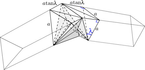
Figure 13: A bend is isometric to a right prism of length $2a\tan\lambda$.

After triangulating the two top quadrilaterals, a bend is made of 20 triangles including the 12 triangles as in Lemma 6.

Rotating a cross section with a gasket

The ribs of the prism $\cal P$ may have only three possible directions. This prevents to bend $\cal P$ in an arbitrary direction. To circumvent this rigidity, Zalgaller introduces a simple construction that he calls a gasket. Consider an equilateral triangle $ABC$ in the horizontal plane and a vertical translate $A^{\prime}B^{\prime}C^{\prime}$ by height $h$. Rotate $A^{\prime}B^{\prime}C^{\prime}$ by an angle $\alpha$ about the central vertical axis. The gasket with turn $\alpha$ and height $h$ is the polyhedral cylinder formed by the six congruent triangles $ABA^{\prime}$, $A^{\prime}BB^{\prime}$, $B^{\prime}BC$, $B^{\prime}CC^{\prime}$, $C^{\prime}CA$, $AA^{\prime}C^{\prime}$. See Figure 14.

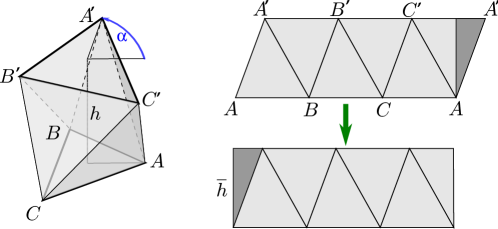
Figure 14: Left, a gasket with turn $\alpha$ and height $h$. Right, the gasket is unfolded in the plane. Cutting and pasting a small triangular piece shows that the gasket has the geometry of a right prism.

This gasket is embedded for every $\alpha\in(-\pi/3,\pi)$, independently of $h>0$.

Lemma 7.

For every $\alpha\in(-\pi/3,\pi)$, the gasket with turn $\alpha$ and height $h$ is isometric to a right prism of length $\bar{h}$ with

$$\bar{h}^{2} =h^{2}+\frac{2}{27}(\sin^{2}\frac{\alpha}{2}+\sin^{2}(\frac{\pi}{3}-\frac{\alpha}{2}))-\frac{4}{81}(\sin^{2}\frac{\alpha}{2}-\sin^{2}(\frac{\pi}{3}-\frac{\alpha}{2}))^{2}-\frac{1}{36}$$ (2)

$$<h^{2}+\frac{1}{9}.$$ (3)

Proof.

By unfolding the gasket in the plane, it is seen to be isometric to a Euclidean rectangle after identifying its vertical sides. See Figure 14. It is thus isometric to a right prism of length $\bar{h}$, where $\bar{h}$ is the height of the rectangle. Fix the coordinates of $A,B,C$ to respectively, $(\frac{1}{3\sqrt{3}},0)$, $(\frac{e^{i2\pi/3}}{3\sqrt{3}},0)$ and $(\frac{e^{-i2\pi/3}}{3\sqrt{3}},0)$ in $\mathbb{R}^{3}=\mathbb{C}\times\mathbb{R}$. Then the coordinates of $A^{\prime},B^{\prime},C^{\prime}$ are respectively $(\frac{e^{i\alpha}}{3\sqrt{3}},h)$, $(\frac{e^{i(\alpha+2\pi/3)}}{3\sqrt{3}},h)$ and $(\frac{e^{i(\alpha-2\pi/3)}}{3\sqrt{3}},h)$. The three sides of the congruent triangles are given by

$$|AB|=1/3,\quad|A^{\prime}A|=\sqrt{\frac{4}{27}\sin^{2}(\alpha/2)+h^{2}},\quad|BA^{\prime}|=\sqrt{\frac{4}{27}\sin^{2}(\pi/3-\alpha/2)+h^{2}}.$$

From Heron’s formula [LL21], we have $\bar{h}=2\frac{\sqrt{p(p-|AB|)(p-|BA^{\prime}|)(p-|A^{\prime}A|)}}{|AB|}$ with $p$ the half-perimeter of $ABA^{\prime}$, and we obtain

$$\bar{h}^{2}=h^{2}+\frac{2}{27}(\sin^{2}\frac{\alpha}{2}+\sin^{2}(\frac{\pi}{3}-\frac{\alpha}{2}))-\frac{4}{81}(\sin^{2}\frac{\alpha}{2}-\sin^{2}(\frac{\pi}{3}-\frac{\alpha}{2}))^{2}-\frac{1}{36}.$$

Since

$$\sin^{2}\frac{\alpha}{2}+\sin^{2}(\frac{\pi}{3}-\frac{\alpha}{2})=\frac{3}{4}-\sin\frac{\alpha}{2}\sin(\frac{\pi}{3}-\frac{\alpha}{2})<7/4,$$

it follows that

$$\bar{h}^{2}<h^{2}+\frac{2}{27}\times\frac{7}{4}-\frac{1}{36}<h^{2}+\frac{1}{9}.$$

∎

By pasting two prisms at the boundaries of a gasket, we obtain a polyhedral cylinder with triangular boundaries, where the two boundaries are turned at the angle $\alpha$ with respect to each other; see Figure 15.

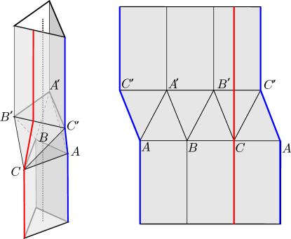
Figure 15: Joining a gasket with two prisms to rotate their ribs. Right, unfolding of the construction showing the line of cut (in blue) and a generatrix (in red) of the polyhedral cylinder.

Note 8.

The top and bottom prisms in Figure 15 have the same central axis. This allows to rotate the rib of a prism at an angle $\alpha\in(\pi/3,\pi)$ before applying a bending.

Note 9.

By joining $k$ gaskets in a row, we can rotate the rib of a prism at an angle $\alpha\in(-k\pi/3,k\pi)$.

Twisting a prism

Replacing a portion of a prism by a gasket with turn $\alpha$ allows to turn one boundary, say the top one, of the prism with respect to the other one but does not twist the prism: the segment connecting a point on a geodesic perpendicular to the bottom boundary (a generatrix) to its closest point on the central axis remains parallel to itself as we move along the geodesic toward the top boundary. In other words, the segment connecting the top endpoint of this geodesic with the top endpoint of the axis will keep the same direction as we augment $\alpha$. In order to twist the prism so that the top endpoint of this geodesic indeed turns with the boundary, Zalgaller introduces yet another construction that he calls a helical twist. This construction takes advantage of the holonomy of parallel transport on the sphere: consider a unit sphere of center $O$ with a spherical triangle $PQR$ (see Figure 16).

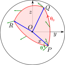
Figure 16: The green tangent vector is transported along the spherical triangle $PQR$. The angle $\theta$ is equal to the area of $PQR$, while the angle $\theta_{0}$ is given by L’Huillier’s formula.

If one parallel transports an object from $P$ to $P$ following the sides of the triangle $PQR$, then the object is rotated by a certain angle around the axis $OP$ which is equal to the signed area of the spherical triangle $PQR$. In order to twist a prism with axis directed by $\overrightarrow{OP}$ by an angle $\theta$ we may thus bend the prism successively in the directions $\overrightarrow{OQ},\overrightarrow{OR}$ and $\overrightarrow{OP}$ again. Each bending at angle $\varphi$ indeed corresponds to a transport along a spherical geodesic of length $\varphi$. Each portion of prism between two bends should include two gaskets to orient its rib properly. Indeed, by Note 9, two gaskets allow to turn by an angle in $(-2\pi/3,2\pi)$, which covers all the possible orientations.

A helical twist of angle $\theta$ consists of a sequence of gaskets and bends according to the pattern $(g^{2}b)^{5}g^{2}=(g^{2}b)^{3}(g^{2}b)^{2}g^{2}$, where $b,g$ stand respectively for bends and gaskets. The prefix $(g^{2}b)^{3}$ in the pattern is used to simulate the parallel transport as described above, assuming that the central axis of the initial cross section is already aligned with $\overrightarrow{OP}$. The next factor $(g^{2}b)^{2}$ allows to return on the central axis of the initial cross section. Since $\overrightarrow{OP}$ is aligned with this central axis, the changes of direction due to the factor $(g^{2}b)^{2}$ happen in the same plane. The resulting holonomy is thus trivial, which ensures that the first and last cross sections of this portion are parallel. Finally, the last two gaskets allows to turn the cross section by any angle in $(-2\pi/3,2\pi]$; see Figure 17.

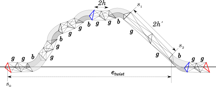
Figure 17: The cross section (in blue) after the last bending of a helical twist is rotated by an angle $\theta$ about the central axis with respect to the initial cross section (in red). The last two gaskets allow to turn the last cross section (in red) to be a translate of the first one.

In practice, to construct a helical twist of angle $\theta\in(-\pi,\pi]$, we choose an equilateral triangle $PQR$ on the unit sphere, with area $\theta$. Moreover, we fix $P=(1,0,0)$, and we take $Q$ in the plane $Oxz$ with positive $z$ coordinate. Then, $R$ is the unique point making $PQR$ equilateral and counterclockwise. Denote by $\theta_{0}$ the angle between the vectors $\overrightarrow{OP}$ and $\overrightarrow{OQ}$. L’Huillier’s formula relates the area $\cal A$ of a geodesic triangle on the unit sphere with its side lengths $a,b,c$ by

$$\tan\frac{\cal A}{4}=\sqrt{\tan\left({\frac{p}{2}}\right)\tan\left({\frac{p-a}{2}}\right)\tan\left({\frac{p-b}{2}}\right)\tan\left({\frac{p-c}{2}}\right)},$$

where $p$ is the half-perimeter. It follows that $\theta_{0}$ satisfies the equation

$$\theta=4\arctan\left(\sqrt{\tan(\frac{3}{4}\theta_{0})\tan^{3}(\frac{\theta_{0}}{4})}\right).$$

Traveling along $PQR$ in trigonometric direction induces a positive rotation angle, while traveling clockwise induces a negative rotation angle. For $|\theta|\leq\pi$, L’Huillier’s formula implies $\theta_{0}\leq 4\arctan\sqrt{2-\sqrt{3}}\approx 1.911$. From (1), we deduce that the corresponding cutting angle satisfies $\lambda\leq\arctan\frac{\sqrt{6-3\sqrt{3}}}{\sqrt{3}-1}<\arctan\frac{49}{40}$. For further reference, we set

$$\lambda_{0}:=\arctan\frac{49}{40}.$$

Denote by $s_{0}$ the initial cross section of the helical twist, by $s_{1}$ the cross section at the end of the fourth bend, and by $s_{2}$ the initial cross section of the last bend. Refer to Figure 17.

Lemma 10.

Given any twist angle $\theta\in(-\pi,\pi]$ and any $h>0$, we can construct a helical twist of angle $\theta$ so that all its bends have cutting angle $\lambda_{0}$, and all its gaskets have height $h$, except the two gaskets between sections $s_{1}$ and $s_{2}$, which have height $h^{\prime}$ imposed by our construction. This helical twist is isometric to a right prism with length

$$\ell_{\text{twist}}=10a\tan\lambda_{0}+10\bar{h}+2\bar{h^{\prime}}$$

and the horizontal distance between the boundaries of the helical twist is bounded by

$$d_{\text{twist}}=18(a\tan\lambda_{0}+h).$$

Here, $\bar{h}$ and $\bar{h^{\prime}}$ are given by Equation (2) in Lemma 7. The height $h^{\prime}$ is moreover bounded by $2\sqrt{10}(2h+3a\tan\lambda_{0})$.

Proof.

Let $a=1/3$ be the length of a rib, i.e., of a side of the triangular cross-sections. The bending angle of the three first bends is equal to $\theta_{0}$ and we know by the previous discussion that they can be realized with the cutting angle $\lambda_{0}$. We need to prove that the last two bends can be realized with this cutting angle. Define the extend $e_{\text{twist}}$ of the helical twist as the horizontal distance between the centers of the sections $s_{0}$ and $s_{2}$. We fix $e_{\text{twist}}=16(h+a\tan\lambda_{0})$. Let $c_{i}$ be the center of $s_{i}$, $i=0,1,2$. The last two bends have the same bending angle $\varphi$, which is the angle between the horizontal direction and the vector $\overrightarrow{c_{1}c_{2}}$. We have $\tan\varphi=\delta_{v}/\delta_{h}$, where $\delta_{v}$ is the distance of $c_{1}$ to the horizontal line through $c_{2}$ and $\delta_{h}$ is the horizontal distance between $c_{1}$ and $c_{2}$. We estimate $\delta_{v}$ by adding the contributions of the eight gaskets and the four bends preceding $s_{1}$. Four of the eight gaskets are horizontal; it follows that they do not contribute to $\delta_{v}$. The fourth bend turns towards the horizontal axis through $c_{2}$, it thus contributes negatively to $\delta_{v}$. We infer that $\delta_{v}\leq 4h+6a\tan\lambda_{0}$. On the other hand, the horizontal distance $d_{01}$ between $c_{0}$ and $c_{1}$ is bounded by $8h+8a\tan\lambda_{0}$. It ensues that $\delta_{h}=e_{\text{twist}}-d_{01}\geq 8h+8a\tan\lambda_{0}$. We conclude that $\tan\varphi\leq(4h+6a\tan\lambda_{0})/(8h+8a\tan\lambda_{0})$. Hence, for all $h$, $\tan\varphi<3/4$. Using Equation (1) and the classical formula $\tan\varphi=2\tan\frac{\varphi}{2}/(1-\tan^{2}\frac{\varphi}{2})$, we deduce $\tan\lambda_{0}(\varphi)<\frac{1}{2\sqrt{3}}$. It follows that $\lambda_{0}(\varphi)<\lambda_{0}$ as desired.

The intrinsic length of the helical twist, i.e., the height of the isometric right cylinder, is the sum of the intrinsic lengths of each constituting bend and gasket. We thus obtain the formula as in the lemma, where $\bar{h}$ and $\bar{h^{\prime}}$ are given by (2). We now remark that the total horizontal extend of the helical twist is bounded by $e_{\text{twist}}+2a\tan\lambda_{0}+2h$ to obtain the bound in the lemma.

We next remark that $d_{01}\geq 4h+2a\tan\lambda_{0}$, taking into account the four horizontal gaskets and the 2 incident horizontal half bends. Hence, $\delta_{h}=e_{\text{twist}}-d_{01}\leq 12h+14a\tan\lambda_{0}$ and we finally conclude

$$h^{\prime}=\sqrt{\delta_{h}^{2}+\delta_{v}^{2}}\leq\sqrt{(12h+14a\tan\lambda_{0})^{2}+(4h+6a\tan\lambda_{0})^{2}}\leq 2\sqrt{10}(2h+3a\tan\lambda_{0}).$$

∎

Putting the pieces together

Consider a flat torus with modulus $\tau=\tau_{1}+i\tau_{i}$. It can be obtained from a right circular cylinder of height $\tau_{i}$ and boundary length 1, identifying the boundaries after a circular shift at angle $2\pi\tau_{1}$. Zalgaller constructs his PL isometric embeddings of long tori, for which $\tau_{i}$ is large, as follows. He first replaces the circular cylinder by an isometric equilateral triangular prism that is bent 6 times at angle $\pi/3$ to form a hexagonal tube. If the torus is rectangular, that is if $\tau_{1}=0$, then the identification of the initial and final cross sections provides the desired embedding. Otherwise, he replaces one side of the hexagon by a helical twist of angle $2\pi\tau_{1}$ in order to glue the boundaries of the prism with the correct angular shift. We use a slightly different construction that allows us to get shorter tori. Starting from a helical twist of angle $\theta$, we add 4 bends at angle $\pi/2$ and 3 portions of right prisms as illustrated on Figure 18

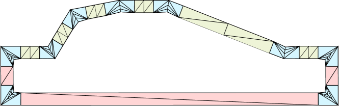
Figure 18: Our construction decomposed into bends (in light blue), gaskets (in light green) and triangular prisms (in pink).

to form a closed torus. In order to avoid intersections between the horizontal prism and the horizontal gaskets of the helical twist we choose the two vertical prisms of length $\frac{a}{3}>\frac{a}{2\sqrt{3}}$. We also choose the length of the horizontal prism to be equal to the total horizontal extend of the helical twist. We finally take the cutting angle of the 3 bends equals to $\lambda_{0}^{\prime}:=\arctan(9/10)>\lambda_{0}(\pi/2)$. The resulting torus has length

$$L<\ell_{\text{twist}}+8a\tan\lambda_{0}^{\prime}+2a/3+d_{\text{twist}}=28a\tan\lambda_{0}+8a\tan\lambda_{0}^{\prime}+2a/3+18h+10\bar{h}+2\bar{h^{\prime}},$$

where $\ell_{\text{twist}}$ and $d_{\text{twist}}$ are given by Lemma 10. Using the bound for $h^{\prime}$ in Lemma 10 together with inequality (3), and the fact that $\tan\lambda_{0}=49/40$, and $\tan\lambda_{0}^{\prime}=9/10$, we get

$$L<\frac{253}{18}+18h+10\sqrt{h^{2}+\frac{1}{9}}+2\sqrt{40(2h+\frac{49}{40})^{2}+\frac{1}{9}}.$$

By taking $h=0$ we thus obtain $L<\frac{253}{18}+\frac{10}{3}+2\sqrt{\frac{49^{2}}{40}+\frac{1}{9}}<33$. Note that any longer torus can be obtained by elongating the two vertical prisms. Hence, for $h$ small enough, we can realize any flat torus of length at least $33$. In practice, our implementation shows that the same construction allows to embed shorter tori. Some rendering is visible on Figure 19.

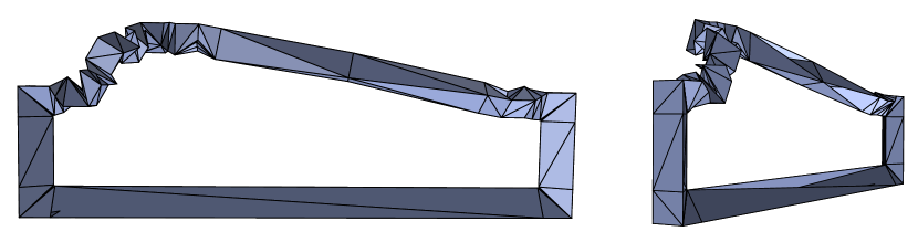
Figure 19: Rendering of the flat torus of length 16 and circular shift $3.5$ corresponding to the modulus $0.558+16i$.

We remark that a prism can be triangulated as a gasket with turn 0, the whole construction thus corresponds to the pattern $(g^{2}b)^{5}g^{2}(bg)^{3}b$ and is composed of $15\times 6+9\times 20=270$ triangles. This ends the proof of Proposition 5. Figure 20 shows the resulting unfolded triangulation after cutting through a cross section and a longitude.

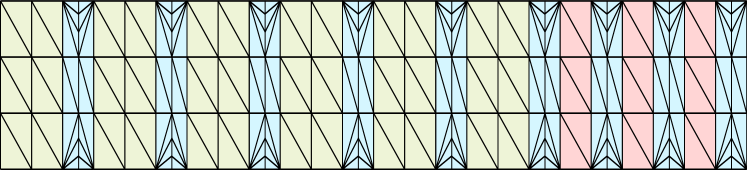
Figure 20: A universal triangulation for long tori.

5.2 The flat tori of Tsuboi and Arnoux et al.

The previous construction provides a universal triangulation for long tori. Referring to Figure 1, this means that the part of the moduli space above the horizontal line $\tau_{i}=33$ can be geometrically realized in $\mathbb{E}^{3}$ by this unique abstract triangulation. It thus remains to cover the compact subspace of short tori below this line. Denote this subspace by ${\cal M}_{\text{short}}$. Hence,

$${\cal M}_{\text{short}}=\{\tau\in\mathbb{H}^{2}\mid|\tau|\geq 1,|\tau_{1}|\leq 1/2,|\tau_{i}|\leq 33\}.$$

As already observed in Section 3, the construction of Burago and Zalgaller allows for some flexibility, implying that around every point in the moduli space there is a neighborhood that can be geometrically realized by the same abstract triangulation. By compactness we can cover ${\cal M}_{\text{short}}$ with a finite number of such neighborhoods. We could thus overlay all the corresponding triangulations with the universal triangulation for long tori to obtain a universal triangulation for all tori. This already provides a proof of the existence of such a triangulation. However, estimating the size of the neighborhoods seems impractical and the approach would lead to a gigantic triangulation. Surprisingly, it was only very recently that Tsuboi [Tsu20] and Arnoux et al. [ALM21] independently (re)discovered extremely simple geometric realizations of flat tori. Arnoux et al. are able to prove that their construction, that they call diplotorus, allows to realize all tori in the moduli space. For completeness we briefly recall this construction.

The diplotorus ${\cal D}_{n,d}^{a,h}$ with parameters $n,d,a,h$ is defined as follows. Let $A_{k}=(e^{i\frac{2\pi k}{n}},0)$ be the vertices of the regular $n$-gon in the horizontal coordinate plane. Let $B_{k}=(e^{i\frac{\pi}{n}(a+1+2k)},h)$ be the vertices of the vertical translate by $h$ of this $n$-gon, turned by an angle $(a+1)\frac{\pi}{n}$. Then ${\cal D}_{n,d}^{a,h}={\cal P}_{\text{int}}\bigcup{\cal P}_{\text{ext}}$ is the union of two twisted prisms, called ploids, where ${\cal P}_{\text{int}}$ is the union of triangles $\{A_{k}A_{k+1}B_{k}\}_{0\leq k<n}$ and $\{B_{k}A_{k+1}B_{k+1}\}_{0\leq k<n}$, and ${\cal P}_{\text{ext}}$ is the union of triangles $\{A_{k}A_{k+1}B_{k-d}\}_{0\leq k<n}$, $\{B_{k-d}A_{k+1}B_{k+1-d}\}_{0\leq k<n}$. Of course, all the indices should be considered modulo $n$. (Note that a ploid with $n=3$ is nothing else but a gasket.) Figure 21 shows the diplotorus ${\cal D}_{5,2}^{3.5,2}$.

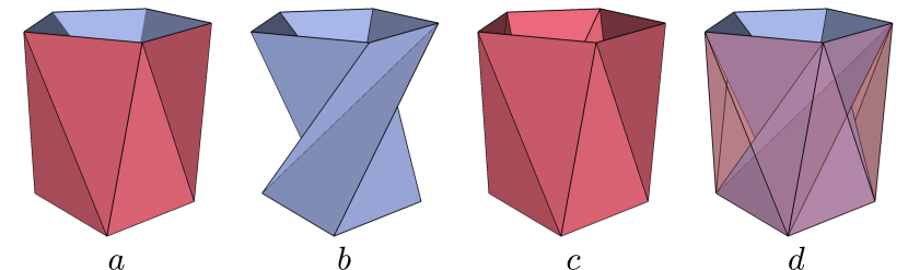
Figure 21: View of the diplotorus ${\cal D}_{5,2}^{3.5,2}$ (a) with its internal (b) and external (c) ploids. (d), another view of ${\cal D}_{5,2}^{3.5,2}$ with a transparent external ploid.

Lemma 11 (Arnoux et al., 2021).

For $h,a\in\mathbb{R}$ and $n,d\in\mathbb{Z}$, ${\cal D}_{n,d,}^{a,h}$ is an embedded flat torus if and only if

$$h>0,n>4,2\leq|d|<n-2,d+1<a<n-1\text{ if }d>0,\quad\text{and}\quad 1-n<a<d-1\text{ if }d<0$$

Moreover, the modulus of ${\cal D}_{n,d}^{a,h}$ is $\tau(n,d,a,h)=\tau_{1}(n,d,a)+i\tau_{i}(n,d,a,h)$ with

$$\tau_{1}(n,d,a)= d/n-\frac{\cos((a-d)\frac{\pi}{n})\sin(d\frac{\pi}{n})}{n\sin\frac{\pi}{n}}\quad\text{and}$$

$$\tau_{i}(n,d,a,h)= \Big{(}\sqrt{h^{2}+4\sin^{2}(\frac{a+1}{2}\cdot\frac{\pi}{n})\sin^{2}(\frac{a-1}{2}\cdot\frac{\pi}{n})}\quad+$$

$$\sqrt{h^{2}+4\sin^{2}(\frac{a-2d+1}{2}\cdot\frac{\pi}{n})\sin^{2}(\frac{a-2d-1}{2}\cdot\frac{\pi}{n})}\,\,\Big{)}/(2n\sin(\pi/n))$$

The map $\tau_{1}$ does not depend on $h$ while $\tau_{i}$ is an increasing function of $h$. It follows that for $n$ and $d$ fixed, the moduli of the tori ${\cal D}_{n,d}^{a,h}$ form a subset of $\mathbb{H}^{2}$, which we denote by ${\cal M}_{n,d}$, that lies above the graph of the parametrized curve $a\mapsto(\tau_{1}(n,d,a),\tau_{i}(n,d,a,0))$, where $a$ varies as in Lemma 11. For $n$ and $d$ fixed, the diplotori in ${\cal D}_{n,d}^{a,h}$ have the same abstract triangulation. If one could cover the moduli space with a finite number of regions ${\cal M}_{n,d}$, this would therefore provide a universal triangulation. This is however impossible and one needs to let $n$ grow to infinity to realize all the rectangular tori. We can nonetheless cover the moduli of short tori with only three regions ${\cal M}_{n,d}$.

5.3 Realizing the short tori with three diplotori

The fundamental domain in Figure 1 is symmetric with respect to the imaginary axis. Two symmetric points $\tau$ and $-\bar{\tau}$ actually represent isometric tori, but the isometry should reverse the orientation. Hence, if $\mathbb{T}_{\tau}$ has a PL isometric embedding in $\mathbb{E}^{3}$ so does $\mathbb{T}_{-\bar{\tau}}$: just take a reflected image of the embedding of $\mathbb{T}_{\tau}$. It is thus enough to realize the positive part ${\cal M}_{\text{short}}^{+}:=\{\tau\in{\cal M}_{\text{short}}\mid\tau_{1}\geq 0\}$ of the short tori to ensure that we can realize all of them.

Remark 2.

From Section 2 the moduli space is the quotient of $\mathbb{H}^{2}$ by the action of $\text{SL}_{2}(\mathbb{Z})$. To realize all the short tori, it is thus sufficient to realize their moduli in any image of ${\cal M}_{\text{short}}^{+}$ under the action of $\text{SL}_{2}(\mathbb{Z})$. Figure 22 shows such an image. The top side $\tau_{i}=33$ of ${\cal M}_{\text{short}}^{+}$ is transformed to an arc of circle, called a horocycle, tangent at 0 to the real axis.

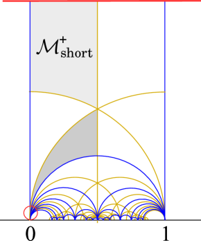
Figure 22: The image (in dark grey) of ${\cal M}_{\text{short}}^{+}$ by the action of $\begin{pmatrix}0&1\\ -1&1\end{pmatrix}\in\text{SL}_{2}(\mathbb{Z})$. The top horizontal line (in red) represents the horocycle $\tau_{i}=33$ (not to scale). Its image by $\begin{pmatrix}0&1\\ -1&1\end{pmatrix}$ is a circle (in red, not to scale) tangent at 0 to the real axis.

Lemma 12.

Any modulus in ${\cal M}_{\text{short}}^{+}$ can be geometrically realized by a diplotorus with parameters $n=19$ and $d\in\{2,7,13\}$.

Proof.

We need to check that ${\cal M}_{\text{short}}^{+}$ is covered by the orbit of ${\cal M}_{19,2}\bigcup{\cal M}_{19,7}\bigcup{\cal M}_{19,13}$ under the action of $\text{SL}_{2}(\mathbb{Z})$. Equivalently, writing $g\cdot{\cal M}_{\text{short}}^{+}$ for the image of ${\cal M}_{\text{short}}^{+}$ by $g\in\text{SL}_{2}(\mathbb{Z})$, we must have that

$$\bigcup_{g\in\text{SL}_{2}(\mathbb{Z})}g^{-1}\cdot\big{(}(g\cdot{\cal M}_{\text{short}}^{+})\bigcap({\cal M}_{19,2}\bigcup{\cal M}_{19,7}\bigcup{\cal M}_{19,13})\big{)}$$

covers ${\cal M}_{\text{short}}^{+}$ (or any of its images). The regions ${\cal M}_{19,2}$ ${\cal M}_{19,7}$ and ${\cal M}_{19,13}$, deduced from the formulas in Lemma 11, are plotted in Figures 23 and 25.

Denote by ${\cal M}^{+}$ the part of the fundamental domain in Figure 1 with non-negative real part. ${\cal M}^{+}$ is bounded by the geodesic triangle with vertices $0,e^{i\pi/3},\infty$. In particular, it contains ${\cal M}_{\text{short}}^{+}$. Consider the subset $\Delta$ of $\text{SL}_{2}(\mathbb{Z})$ composed of the matrices $g_{\delta}:=\begin{pmatrix}0&1\\ -1&\delta\end{pmatrix}$ with $\delta$ a positive integer. The elements in $\Delta$ transform ${\cal M}^{+}$ into a fan of triangular domains with positive real part, tangent at 0 to the imaginary axis. They moreover transform each horocycle $\{\tau_{i}=\text{constant}\}$ into a same circle tangent at 0 to the real axis. Larger constants give rise to smaller circles.

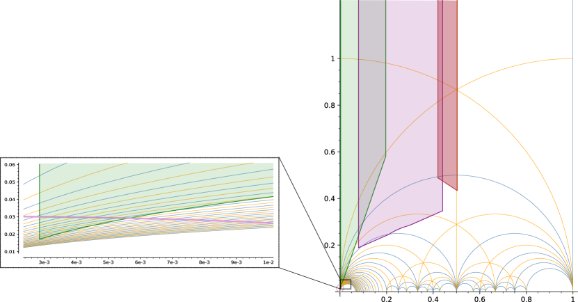
Figure 23: The moduli space for ${\cal M}_{19,2}$ (in green), ${\cal M}_{19,7}$ (in purple), and ${\cal M}_{19,13}$ (in red). The axes in the bottom enlargement have different scales; the horocycle (thick purple line), image of $\{\tau_{i}=33\}$ by the elements of $\Delta$, appear as an arc of ellipse.

Two such circles cut the transforms of ${\cal M}^{+}$ by $\Delta$ into slices that are themselves transforms of a same slice in ${\cal M}^{+}$. Figures 24 and 25 demonstrates that we can slice ${\cal M}_{\text{short}}^{+}$ so that each slice has a transform by respectively $g_{1},g_{3},g_{5}$ (in yellow, blue, and red on the figure) covered by ${\cal M}_{19,2}\bigcup{\cal M}_{19,7}\bigcup{\cal M}_{19,13}$.

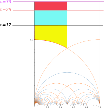
Figure 24: A slicing of ${\cal M}_{\text{short}}^{+}$ (not to scale) in three regions (yellow, blue and red) by the horocycles $\tau_{i}=33,25,12$ (respectively in purple, orange, and black) and the geodesic unit circle.

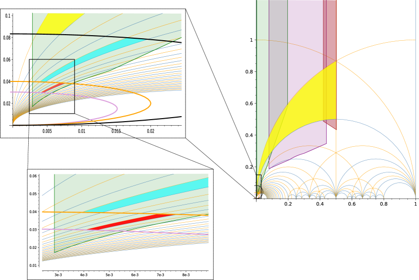
Figure 25: The three regions in red, blue and yellow are images of the corresponding slices in ${\cal M}_{\text{short}}^{+}$ by $g_{1},g_{3},g_{5}$, respectively.

It follows that

$${\cal M}_{\text{short}}^{+}\subset\bigcup_{\delta\in\{1,3,5\}}g_{\delta}^{-1}\cdot\big{(}(g_{\delta}\cdot{\cal M}_{\text{short}}^{+})\bigcap({\cal M}_{19,2}\bigcup{\cal M}_{19,7}\bigcup{\cal M}_{19,13})\big{)},$$

which proves the lemma. This proof by picture can be made formal by computing the exact arrangement of the involved domains, whose boundary are made of arcs of circles and lines segments. The details are provided in Appendix. ∎

From Lemma 12 we can construct a universal triangulation for short tori. Indeed, all the diplotori with fixed parameters $n,d$ have the same abstract triangulation, that we denote by ${\cal T}_{n,d}$. Hence, we just need a common subdivision of ${\cal T}_{19,2}$, ${\cal T}_{19,7}$ and ${\cal T}_{19,13}$ to obtain such a universal triangulation. These triangulations are obtained by identifying the boundaries of a same triangulated cylinder. However, they are not isomorphic, as one needs to apply distinct circular shifts before identification. We can nonetheless send them in a same torus as follows. For $k\in\mathbb{Z}$, consider the points

$$A_{k}=(k,-1),\quad B_{k}=(k,0),\quad C_{k}=(k,1)$$

in the infinite plane strip ${\cal B}:=\mathbb{R}\times[-1,1]$. Then, ${\cal T}_{19,d}$ is isomorphic to the triangulation of $\cal B$ by the triangles $\{A_{k}A_{k+1}B_{k},B_{k}A_{k+1}B_{k+1},C_{k}C_{k+1}B_{k-d},B_{k-d}C_{k+1}B_{k+1-d}\}_{k\in\mathbb{Z}}$ quotiented by the horizontal translations generated by the vector $(19,0)$, further identifying the two boundaries according to the vertical translation $(0,2)$. This quotient and identification being independent of $d$, the three triangulations for $d=2,7,13$ are indeed embedded in a same torus; see Figure 26.

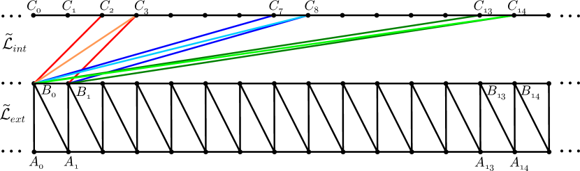
Figure 26: Layout of the triangulations ${\cal T}_{19,2}$, ${\cal T}_{19,7}$ and ${\cal T}_{19,13}$. The two sub-strips $\tilde{{\cal L}}_{\text{int}}$ and $\tilde{{\cal L}}_{\text{ext}}$ correspond to the (lift of) overlay of the internal and external ploids.

We overlay the three triangulated strips obtained for $d=2,7,13$. We want to count the number of vertices of the resulting subdivision. We only have to care about the edges $B_{k}C_{\ell}$, the other ones being common to the three triangulations. By symmetry it suffices to consider the number of intersections with the other edges of the six edges $B_{0}C_{k}$ for $k\in I:=\{2,3,7,8,13,14\}$. The edges $B_{0}C_{k}$ and $B_{\ell}C_{\ell+j}$, $j\in I$, intersect in their interior if and only if

• $\ell<0$ and $\ell+j>k$, or equivalently $k-j<\ell<0$, or

• $\ell>0$ and $\ell+j<k$, or equivalently $0<\ell<k-j$.

In this case, we compute $p_{\ell,j}^{k}:=B_{0}C_{k}\bigcap B_{\ell}C_{\ell+j}=\frac{\ell}{k-j}(k,1)$. All other intersection points are horizontal translates of the $p_{\ell,j}^{k}$ by an integral amount. The set of intersection points with $x$-coordinate in $[0,1)$ is thus given by $\{\text{frac}(\frac{\ell k}{k-j}),\frac{\ell}{k-j})\}_{j,k,\ell}$, where $j,k,\ell$ vary as above and $\text{frac}(x)$ is the fractional part of $x$. Eliminating the duplicates, we found 56 intersections leading to $n\times 56=1064$ intersection points in total. Adding the remaining points $A_{k},B_{k}$ ($C_{k}$ and $A_{k}$ should be identified) we find a total of $1064+38=1102$ vertices. It remains to triangulate the subdivision by adding diagonals in the non triangular faces. By Euler’s formula on the torus, we conclude that the triangulated overlay has 2204 triangles. We have thus proved

Proposition 13.

There exists an abstract triangulation with 2204 triangles, which admits linear embeddings isometric to every short torus.

6 Merging short and long tori

It remains to overlay our universal triangulations for long and short tori to obtain a universal triangulation for all tori. Before overlaying the layouts of Figures 20 and 26, we perform some modifications. We first remove the diagonals introduced to triangulate the rectangular faces of the bends as they are not necessary to define the isometric PL embeddings of long tori. For the same reason, we remove the diagonals used to triangulate the three portions of right prisms; Compare Figure 20 and top Figure 27.

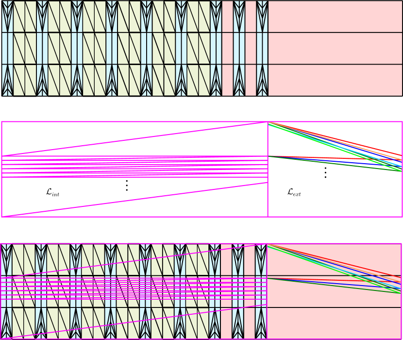
Figure 27: Modified layout of the universal triangulations for long and short tori, and their overlay.

Denote by ${\cal L}_{\text{long}}$ the resulting layout. It is composed of three horizontal strips, where the central one has no internal vertex and is traversed by $E_{c}=45$ edges (the leftmost and rightmost edges should be identified) corresponding to 9 bends, 12 gaskets, and 3 portions of right prisms. We next apply a quarter turn to the layout for short tori, call it ${\cal L}_{\text{short}}$. It decomposes into two parts ${\cal L}_{\text{int}}\bigcup{\cal L}_{\text{ext}}$ corresponding to the internal and external ploids; compare Figure 26 with middle of Figure 27. We apply some stretching and compression in order to align ${\cal L}_{\text{ext}}$ with the rightmost portion of right prism in ${\cal L}_{\text{long}}$. We also move vertically the vertices of ${\cal L}_{\text{short}}$ that are not on the horizontal boundaries of the layout, so that they fit in the central horizontal strip of ${\cal L}_{\text{long}}$. We are now ready to overlay ${\cal L}_{\text{short}}$ and ${\cal L}_{\text{long}}$ as shown at the bottom of Figure 27. Note that the (universal) subdivisions for short and long tori are obtained from the corresponding layouts by applying the same identifications of their horizontal and vertical sides. Applying these identifications to the overlay of the layouts thus provides a common refinement of the subdivisions for short and long tori. We enumerate the vertices of the overlay as follows. It contains

• $V_{\cap}=1064$ vertices from the intersecting edges in ${\cal L}_{\text{short}}$ as computed in the proof of Proposition 13,

• $3V_{\text{ext}}$ vertices, where $V_{\text{ext}}$ is the number of intersections in ${\cal L}_{\text{ext}}$ of a horizontal edge of ${\cal L}_{\text{long}}$ with the edges of ${\cal L}_{\text{short}}$,

• $V_{\text{long}}=270/2=135$ vertices from the triangulation of long tori,

• $(2n-3)V_{c}=35V_{c}$ vertices in the central horizontal strip, where $V_{c}$ is the number of intersections of an edge of ${\cal L}_{\text{int}}$ in this strip with the edges of ${\cal L}_{\text{long}}$,

• $V_{d}$ intersections of the two remaining diagonals of ${\cal L}_{\text{int}}$ with the edges of ${\cal L}_{\text{long}}$.

A horizontal line in ${\cal L}_{\text{ext}}$ with ordinate $y$ intersects all the edges $B_{\ell}C_{\ell+j}$ such that $y\in(\ell,\ell+j)$. This gives $V_{\text{ext}}=\sum_{j\in I}(j-1)=41$. Since every edge of ${\cal L}_{\text{int}}$ contained in the central horizontal strip of ${\cal L}_{\text{long}}$ intersects all its edges, we have $V_{c}=E_{c}=45$. It remains to count the intersections with the last two diagonals of ${\cal L}_{\text{int}}$ contained respectively in the top and bottom strips of ${\cal L}_{\text{long}}$. Rather than considering these diagonals as straight line segments, we artificially subdivide each of them by adding a vertex close to their extremities, moving it to the boundary of the central strip; see Figure 28.

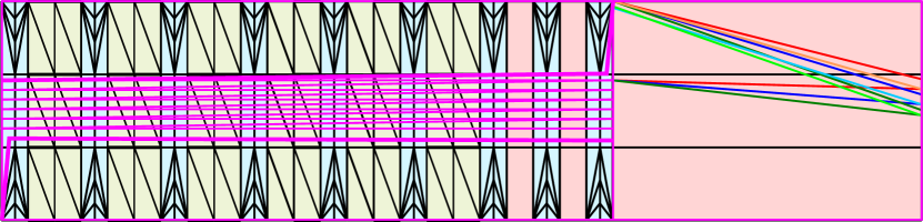
Figure 28: The subdivision of the remaining two diagonals of ${\cal L}_{\text{long}}$ (thick purple lines).

This introduces $V_{c}$ vertices per diagonal, so that $V_{d}=90$. In total the overlay thus contains

$$V_{\cap}+3V_{\text{ext}}+V_{\text{long}}+35V_{c}+V_{d}=1064+3\times 41+135+35\times 45+90=2987$$

vertices. By Euler’s formula this corresponds, after adding diagonals to triangulate the overlay, to 5974 triangles. This ends the proof of Theorem 1.

Our construction is clearly not optimal. The size of our universal triangulation for long tori can probably be reduced, say by simplifying the helical twist. The choice of the diplotori to realize the short tori may also be optimized to reduce the size of the resulting triangulation. Finally, the overlay of these triangulations can also be optimized. A challenging question is to find the smallest number of triangles in a universal triangulation for flat tori.

Appendix

Here, we provide the details for the proof of Lemma 12. From Lemma 11, simple computations show that the region ${\cal M}_{19,2}$ is bounded by the following curves:

• $\lambda_{2}(t)=z_{2}+it$ with $t\in[0,+\infty[$ and $z_{2}=\frac{2-\sin\frac{2\pi}{19}\cot\frac{\pi}{19}+i\sin\frac{2\pi}{19}}{19}$,

• $\beta_{2,1}(t)=\frac{2}{19}-\frac{\sin\frac{2\pi}{19}}{19\sin\frac{\pi}{19}}e^{-it}$ with $t\in[\frac{\pi}{19},\frac{3\pi}{19}]$,

• $\beta_{2,2}(t)=\frac{2+i\cot\frac{\pi}{19}}{19}-\frac{e^{i\frac{15\pi}{38}}}{19\sin\frac{\pi}{19}}t$ with $t\in[\cos\frac{16\pi}{19},\cos\frac{3\pi}{19}]$,

• $\rho_{2}(t)=w_{2}+it$ with $t\in[0,+\infty[$ and $w_{2}=\beta_{2,2}\left(\cos\frac{16\pi}{19}\right)$.

While $\mathcal{M}_{19,7}$ is bounded by:

• $\lambda_{7}(t)=z_{7}+it$ with $t\in[0,+\infty[$ and $z_{7}=\frac{7-\sin\frac{7\pi}{19}\cot\frac{\pi}{19}+i\cot\frac{\pi}{19}\left(1-\cos\frac{7\pi}{19}\right)}{19}$,

• $\beta_{7,1}(t)=\frac{7+i\cot\frac{\pi}{19}}{19}-\frac{e^{i\frac{5\pi}{38}}}{19\sin\frac{\pi}{19}}t$ with $t\in[\cos\frac{6\pi}{19},\cos\frac{\pi}{19}]$,

• $\beta_{7,2}(t)=\frac{7}{19}-\frac{\sin\frac{7\pi}{19}}{19\sin\frac{\pi}{19}}e^{-it}$ with $t\in[\frac{6\pi}{19},\frac{8\pi}{19}]$,

• $\beta_{7,3}(t)=\frac{7+i\cot\frac{\pi}{19}}{19}-\frac{e^{i\frac{5\pi}{38}}}{19\sin\frac{\pi}{19}}t$ with $t\in[\cos\frac{11\pi}{19},\cos\frac{8\pi}{19}]$,

• $\rho_{7}(t)=w_{7}+it$ with $t\in[0,+\infty[$ and $w_{7}=\beta_{7,3}\left(\cos\frac{11\pi}{9}\right)$.

And $\mathcal{M}_{13}$ is bounded by:

• $\lambda_{13}(t)=z_{13}+it$ with $t\in[0,+\infty[$ and $z_{13}=\frac{13-\sin\frac{13\pi}{19}\cot\frac{\pi}{19}+i\cot\frac{\pi}{19}\left(1-\cos\frac{13\pi}{19}\right)}{19}$,

• $\beta_{13,1}(t)=\frac{13+i\cot\frac{\pi}{19}}{19}-\frac{e^{-i\frac{7\pi}{38}}}{19\sin\frac{\pi}{19}}t$ with $t\in[\cos\frac{5\pi}{19},\cos\frac{\pi}{19}]$,

• $\rho_{13}(t)=w_{13}+it$ with $t\in[0,+\infty[$ and $w_{13}=\beta_{13,1}\left(\cos\frac{5\pi}{19}\right)$.

In the sequel we denote by $\mathcal{B}(z,r)$ the closed disk of radius $r$ centered at $z$ and by $\mathcal{C}(z,r)$ its boundary circle. We also denote by $\Re(z)$ and $\Im(z)$, the real part and the imaginary part of $z$, respectively. Recall that each $g_{\delta}:z\mapsto\frac{1}{-z+\delta}$ sends the horizontal line $\{\Im(z)=h\}$ onto the circle $\mathcal{C}(\frac{i}{2h},\frac{1}{2h})$. Furthermore, for $\delta\geq 1$, $g_{\delta}$ sends the imaginary axis onto the circle $\mathcal{C}(\frac{1}{2\delta},\frac{1}{2\delta})$, and the line $\{\Re(z)=\frac{1}{2}\}$ onto the circle $\mathcal{C}(\frac{1}{2\delta-1},\frac{1}{2\delta-1})$. We denote the red, blue and yellow slices of ${\cal M}^{+}_{\text{short}}$ on Figure 24 by respectively ${\cal S}_{r}$, ${\cal S}_{b}$ and ${\cal S}_{y}$.

From these facts, we deduce that $g_{5}({\cal S}_{r})$, the image of the red slice by $g_{5}$ (see Figure 25), is bounded by four arcs of circles; one from respectively $\mathcal{C}(\frac{1}{9},\frac{1}{9}),\mathcal{C}(\frac{i}{66},\frac{1}{66}),\mathcal{C}(\frac{1}{10},\frac{1}{10})$ and $\mathcal{C}(\frac{i}{50},\frac{1}{50})$. Similarly, the image $g_{3}({\cal S}_{b})$ of the blue slice is bounded by arcs from the circles $\mathcal{C}(\frac{1}{5},\frac{1}{5}),\mathcal{C}(\frac{i}{50},\frac{1}{50}),\mathcal{C}(\frac{1}{6},\frac{1}{6})$ and $\mathcal{C}(\frac{i}{24},\frac{1}{24})$. Finally, the image $g_{1}({\cal S}_{y})$ of the yellow slice is bounded by arcs of the circles $\mathcal{C}(1,1),\mathcal{C}(\frac{i}{24},\frac{1}{24}),\mathcal{C}(\frac{1}{2},\frac{1}{2})$ and a segment of the line $\{\Re(z)=\frac{1}{2}\}$. For this last slice, we note that $g_{1}$ sends the arc of circle $\{e^{it}\mid\frac{\pi}{3}\leq t\leq\frac{\pi}{2}\}$ to the vertical line segment $\{\frac{1}{2}+it\mid t\in[\frac{1}{2},\frac{\sqrt{3}}{2}]\}$.

We now proceed to prove that the three curvilinear quadrilaterals $g_{5}({\cal S}_{r})$, $g_{3}({\cal S}_{b})$ and $g_{1}({\cal S}_{y})$ shown in Figure 25 lie above the lower boundary of $\mathcal{M}_{19}:=\mathcal{M}_{19,2}\cup\mathcal{M}_{19,7}\cup\mathcal{M}_{19,13}$. (A point $z$ lies above another point $w$ with same real part if $\Im(z)\geq\Im(w)$.) Let us remark that for showing that such a quadrilateral lies above some boundary, it suffices to show that the bottom side and the right most side of the quadrilateral lie above this boundary as the quadrilateral is completely included in the region of the plane above these two sides.

The Red quadrilateral $g_{5}({\cal S}_{r})$.

Denote the vertices of this quadrilateral as in Figure 29. From the above description, one computes $A_{1}=\frac{6+44i}{1479},A_{2}=\frac{5+33i}{1114},A_{3}=\frac{1+5i}{130},A_{4}=\frac{18+100i}{2581}$. By the previous remark it is enough to show that the curvilinear sides $\overset{\frown}{A_{1}A_{2}}$ and $\overset{\frown}{A_{2}A_{3}}$ lie above the lower boundary of $\mathcal{M}_{19}$.

Figure 29: The red quadrilateral $A_{1}A_{2}A_{3}A_{4}$

• Arc $\overset{\frown}{A_{1}A_{2}}$.

  The vertical line through $\beta_{2,1}(t)$ cuts $\mathcal{C}(\frac{i}{66},\frac{1}{66})$ (the circle containing $\overset{\frown}{A_{1}A_{2}}$) in two points. We denote by $P_{1}(t)$ the highest of these two points. Remark that $\overset{\frown}{A_{1}A_{2}}$ is indeed in the upper half part of $\mathcal{C}(\frac{i}{66},\frac{1}{66})$. We compute $P_{1}(t)=\frac{i+e^{i\tau}}{66}$ with $0\leq\tau\leq\pi$, where $\frac{\cos\tau}{66}=\frac{2}{19}-\frac{\sin\frac{2\pi}{19}}{19\sin\frac{\pi}{19}}\cos t$. Thus:

  $$\Im(P_{1}(t))=\frac{1+\sin\tau}{66}\geq\Im(\beta_{2,1}(t))=\frac{\sin\frac{2\pi}{19}}{19\sin\frac{\pi}{19}}\sin t$$

  $$\iff\frac{\sin^{2}\tau}{66^{2}}\geq\left(-\frac{1}{66}+\frac{\sin\frac{2\pi}{19}}{19\sin\frac{\pi}{19}}\sin t\right)^{2}$$

  $$\iff f_{1}(\cos t)\geq 0,$$

  where,

  $$f_{1}(x):=\frac{8x}{361}\cos\frac{\pi}{19}+\frac{2\sqrt{1-x^{2}}}{627}\cos\frac{\pi}{19}-\frac{6+2\cos\frac{2\pi}{19}}{361}$$

  A study of $f_{1}$ shows that it is non negative on $[0.96,1]$, so that $f_{1}(\cos t)$ is non negative for $t\in[0,t_{red}^{1}:=0.283]$. Note that $0<\pi/19<t_{red}^{1}<3\pi/19$. Moreover, $\Re(z_{2}=\beta_{2,1}(\frac{\pi}{19}))\approx 0.002<\Re(A_{1})=\frac{6}{1479}$ and $\Re(\beta_{2,1}(t_{red}^{1}))\approx 0.0055>\Re(A_{2})=\frac{5}{1114}$. This shows that the arc $\overset{\frown}{A_{1}A_{2}}$ entirely lies above $\beta_{2,1}$.

• Arc $\overset{\frown}{A_{2}A_{3}}$.

  The vertical line through $\beta_{2,1}(t)$ cuts $\mathcal{C}(\frac{1}{10},\frac{1}{10})$ (the circle containing $\overset{\frown}{A_{2}A_{3}}$) in two points. Denoting by $P_{2}(t)$ the highest of these two points, similar computations as above lead to:

  $$\Im(P_{2}(t))\geq\Im(\beta_{2,1}(t))\iff f_{2}(\cos t):=\frac{1}{1805}\frac{\sin\frac{2\pi}{19}}{\sin\frac{\pi}{19}}\cos t+\frac{18}{1805}-\frac{\sin^{2}\frac{2\pi}{19}}{361\sin^{2}\frac{\pi}{19}}\geq 0.$$

  Since $f_{2}$ is non negative on $[0.55,1]$, we have that $f_{2}(\cos t)$ is non negative for $t\in[0,0.9]$. Note that this interval contains the interval of definition $[\frac{\pi}{19},\frac{3\pi}{19}]$ of $\beta_{2,1}$. Since $\Re(z_{2})<\Re(A_{2})$ and $\Re(\beta_{2,1}(\frac{3\pi}{19}))\approx 0.014>\Re(A_{3})=\frac{1}{130}$, the arc $\overset{\frown}{A_{2}A_{3}}$ is included in the region above $\beta_{2,1}$. We thus conclude that $A_{1}A_{2}A_{3}A_{4}$ lies entirely above $\beta_{2,1}$.

The blue quadrilateral $g_{3}({\cal S}_{b})$.

Denote the vertices of this quadrilateral $B_{1},B_{2},B_{3},B_{4}$ in analogy with what precedes ($B_{1}$ is the bottom left vertex of the quadrilateral, $B_{2}$ the bottom right one, $B_{3}$ the top right one and $B_{4}$ the top left one). We compute $B_{1}=\frac{2+20i}{505},B_{2}=\frac{3+25i}{634},B_{3}=\frac{1+4i}{51},B_{4}=\frac{10+48i}{601}$. Again, it is enough to show that the curvilinear sides $\overset{\frown}{B_{1}B_{2}}$ and $\overset{\frown}{B_{2}B_{3}}$ lie above the lower boundary of $\mathcal{M}_{19}$.

• Arc $\overset{\frown}{B_{1}B_{2}}$.

  The vertical line passing by $\beta_{2,1}(t)$ cuts $\mathcal{C}(\frac{i}{50},\frac{1}{50})$ (the circle containing $\overset{\frown}{B_{1}B_{2}}$) in two points. Let $Q_{1}(t)$ denotes the highest of these two points. We have

  $$\Im(Q_{1}(t)) \geq\Im(\beta_{2,1}(t))\iff$$

  $$f_{3}(\cos t) :=\frac{4\sin\frac{2\pi}{19}}{361\sin\frac{\pi}{19}}\cos t+\frac{\sin\frac{2\pi}{19}}{475\sin\frac{\pi}{19}}\sqrt{1-\cos^{2}t}-\frac{4}{361}-\frac{\sin^{2}\frac{2\pi}{19}}{361\sin^{2}\frac{\pi}{19}}\geq 0.$$

  Furthermore, $f_{3}$ is non negative on $[0.94,1]$, so that $f_{3}(\cos t)$ is non negative on $[0,t_{blue}^{1}:=0.3]$. Note that $0<\pi/19<0.3<3\pi/19$. Moreover, $\Re(z_{2})\approx 0.002<\Re(B_{1})=\frac{2}{505}$ and $\Re(\beta_{2,1}(t_{blue}^{1}))\approx 0.008>\Re(B_{2})=\frac{3}{634}$, which implies that $\overset{\frown}{B_{1}B_{2}}$ lies entirely above $\beta_{2,1}$.

• Arc $\overset{\frown}{B_{2}B_{3}}$.

  Denote by $Q_{2}(t)$ the highest intersection point of the vertical line passing through $\beta_{2,1}(t)$ with $\mathcal{C}(\frac{1}{6},\frac{1}{6})$ (the circle containing $\overset{\frown}{B_{2}B_{3}}$). We have

  $$\Im(Q_{2}(t))\geq\Im(\beta_{2,1}(t))\iff f_{4}(\cos t):=-\frac{7\sin\frac{2\pi}{19}}{1083\sin\frac{\pi}{19}}\cos t+\frac{26}{1083}-\frac{\sin^{2}\frac{2\pi}{19}}{361\sin^{2}\frac{\pi}{19}}\geq 0.$$

  Since $f_{4}$ is non negative on $[-1,1]$ and $\Re(z_{2})<\Re(B_{2})$, it follows that $\overset{\frown}{B_{2}B_{3}}$ is above $\beta_{2,1}$ over the interval $[\Re(B_{2}),\Re(\beta_{2,1}(\frac{3\pi}{19}))]$. Let $\overline{\beta}_{2,2}$ be the supporting line of $\beta_{2,2}$. The point of $\overline{\beta}_{2,2}$ on the same vertical as $B_{2}$ is $Q_{3}:=\beta_{2,2}\left(\frac{1211\sin\frac{\pi}{19}}{634\cos\frac{15\pi}{38}}\right)$, while the point of $\beta_{2,2}$ on the same vertical line as $B_{3}$ is $Q_{4}:=\beta_{2,2}\left(t_{blue}^{2}:=\frac{83\sin\frac{\pi}{19}}{51\cos\frac{15\pi}{38}}\right)$. Observe that $t_{blue}^{2}\in[\cos\frac{16\pi}{19},\cos\frac{3\pi}{19}]$. We compute $\Im(Q_{3})\approx 0.02<\Im(B_{2})=\frac{25}{634}$ and $\Im(Q_{4})\approx 0.06<\Im(B_{3})=\frac{4}{51}$. By concavity of $\overset{\frown}{B_{2}B_{3}}$, we deduce that $\overset{\frown}{B_{2}B_{3}}$ lies above $\beta_{2,2}$ over $[\Re(\beta_{2,2}(\cos\frac{3\pi}{19})),\Re(B_{3})]$. We conclude that $\overset{\frown}{B_{2}B_{3}}$ lies above $\beta_{2,1}\cup\beta_{2,2}$.

The yellow quadrilateral $g_{1}({\cal S}_{y})$.

Denote the vertices of this quadrilateral $C_{1},C_{2},C_{3},C_{4}$ analogously to what precedes. One computes

$$C_{1}=\frac{2+48i}{577},C_{2}=\frac{1+12i}{145},C_{3}=\frac{1+i}{2},C_{4}=\frac{1+\sqrt{3}i}{2}=e^{i\frac{\pi}{3}}.$$

We show that the curvilinear sides $\overset{\frown}{C_{1}C_{2}}$ and $\overset{\frown}{C_{2}C_{3}}$ lie above the lower boundary of $\mathcal{M}_{19}$.

• Arc $\overset{\frown}{C_{1}C_{2}}$.

  Let $R_{1}(t)$ be the highest intersection point of the vertical through $\beta_{2,1}(t)$ with $\mathcal{C}(\frac{i}{24},\frac{1}{24})$ (the circle containing $\overset{\frown}{C_{1}C_{2}}$). We have

  $$\Im(R_{1}(t)) \geq\Im(\beta_{2,1}(t))\iff$$

  $$f_{5}(\cos t) :=\frac{8\cos\frac{\pi}{19}}{361}\cos t+\frac{\cos\frac{\pi}{19}}{114}\sqrt{1-\cos^{2}t}-\frac{6+2\cos\frac{2\pi}{19}}{361}\geq 0.$$

  Since $f_{5}$ is non negative on $[0.8,1]$, it ensues that $f_{5}(\cos t)$ is non negative for $t$ in $[0,0.6]$. This interval contains $[\frac{\pi}{19},\frac{3\pi}{19}]$. As $\Re(z_{2})\approx 0.002<\Re(C_{1})=\frac{2}{577}$ and $\Re(\beta_{2,1}(\frac{3\pi}{19}))\approx 0.02>\Re(C_{2})=\frac{1}{145}$, we conclude that $\overset{\frown}{C_{1}C_{2}}$ lies entirely above $\beta_{2,1}$.

• Arc $\overset{\frown}{C_{2}C_{3}}$.

  First we note that if a point $z$ with $\Re(C_{3})\leq\Re(z)\leq\frac{1}{2}$ belongs to $\mathcal{B}(\frac{1}{2},\frac{1}{2})$ then it lies below the arc $\overset{\frown}{C_{2}C_{3}}$. Thus to show that $\beta_{i,j}(t)$ is below $\overset{\frown}{C_{2}C_{3}}$ it is sufficient to show that $|\beta_{i,j}(t)-\frac{1}{2}|\leq\frac{1}{2}$.

  We have

  $$|\beta_{2,1}(t)-\frac{1}{2}|\leq\frac{1}{2}\iff f_{6}(\cos t):=\frac{15\sin\frac{2\pi}{19}}{361\sin\frac{\pi}{19}}\cos t+\frac{\sin^{2}\frac{2\pi}{19}}{361\sin^{2}\frac{\pi}{19}}-\frac{34}{361}\leq 0.$$

  Since $f_{6}$ is non positive on $[-1,1]$, it follows that $f_{6}(\cos t)$ is always non positive. Hence $\overset{\frown}{C_{2}C_{3}}$ is above $\beta_{2,1}$ over $[\Re(C_{2}),\Re(\beta_{2,1}(\frac{3\pi}{19}))]$.

  Next, we show that $\overset{\frown}{C_{2}C_{3}}$ lies above $\beta_{2,2}$ in the strip $\{z\mid\Re(z)\in[\Re(\beta_{2,1}(\frac{3\pi}{19})),\Re(z_{7})]\}$. Let $R_{2,7}$ be the point on $\beta_{2,2}$ with real part $\Re(z_{7})$. We have
  $R_{2,7}=\beta_{2,2}\left(\tau_{2,7}:=\frac{(-5+\cos\frac{5\pi}{38}\cot\frac{\pi}{19})\sin\frac{\pi}{19}}{\sin\frac{2\pi}{19}}\right)$ and we verify that $\tau_{2,7}\in[\cos\frac{16\pi}{19},\cos\frac{3\pi}{19}]$ and $\Im R_{2,7}\approx 0.24>\Im z_{7}\approx 0.18$. Then, to show that $\overset{\frown}{C_{2}C_{3}}$ lies above $\beta_{2,2}$ in the above strip, it suffices by concavity of $\mathcal{B}(\frac{1}{2},\frac{1}{2})$ (as $\beta_{2,2}$ is a line segment) to show that $\beta_{2,2}(\cos\frac{3\pi}{19}),R_{2,7}\in\mathcal{B}(\frac{1}{2},\frac{1}{2})$. We indeed compute: $|\beta_{2,2}(\cos\frac{3\pi}{19})-\frac{1}{2}|^{2}\approx 0.23<\frac{1}{4}$, $|R_{2,7}-\frac{1}{2}|^{2}\approx 0.23<\frac{1}{4}$.

  It remains to show that the lower boundaries of $M_{19,7}$ and $M_{19,13}$ lie below $\overset{\frown}{C_{2}C_{3}}$ in the strip $\{z\mid\Re(z)\in[\Re(z_{7}),\Re(C_{3})=1/2]\}$.

  We have

  $$|\beta_{7,1}(t)-\frac{1}{2}|^{2}=|\beta_{7,3}(t)-\frac{1}{2}|^{2}\leq\frac{1}{4}\iff$$

  $$f_{7}(t):=\frac{\cos^{2}\frac{5\pi}{38}}{361\sin^{2}\frac{\pi}{19}}t^{2}+\frac{5\cos\frac{5\pi}{38}}{361\sin\frac{\pi}{19}}t-\frac{84}{361}+\frac{\cos^{2}\frac{\pi}{19}+\cos\frac{\pi}{19}\sin\frac{5\pi}{38}+\sin^{2}\frac{5\pi}{38}}{361\sin^{2}\frac{\pi}{19}}\leq 0.$$

  As $f_{7}$ is non positive on the interval $[-1,1]$, which contains the domains of $\beta_{7,1}$ and $\beta_{7,3}$, we deduce that these two curves lie entirely below $\overset{\frown}{C_{2}C_{3}}$.

  We then have

  $$|\beta_{7,2}(t)-\frac{1}{2}|^{2}\leq\frac{1}{4}\iff f_{8}(\cos t):=\frac{5\cos\frac{5\pi}{38}}{361\sin\frac{\pi}{19}}\cos t-\frac{84}{361}+\frac{\cos^{2}\frac{5\pi}{38}}{361\sin^{2}\frac{\pi}{19}}\leq 0.$$

  Since $f_{8}$ is non positive on $[-1,1]$, it follows that $f_{8}(\cos t)$ is non positive for all $t$, which shows that $\beta_{7,2}$ lies below $\overset{\frown}{C_{2}C_{3}}$.

  Finally, as previously noticed, since $\beta_{13,1}$ is a line segment, it suffices to show that its extremities lies below $\overset{\frown}{C_{2}C_{3}}$ by concavity. We compute: $|z_{13}-\frac{1}{2}|^{2}\approx 0.244<\frac{1}{4}$ and $|w_{13}-\frac{1}{2}|\approx 0.1<\frac{1}{4}$. Thus $\overset{\frown}{C_{2}C_{3}}$ lies above $\beta_{13,1}$, and as $\Re(w_{13})\approx 0.502>\frac{1}{2}=\Re(C_{3})$, we deduce that $\overset{\frown}{C_{2}C_{3}}$ is included in $M_{19}$.

This ends the proof of Lemma 12.

References

- [ALM21] Pierre Arnoux, Samuel Lelièvre, and Alba Málaga. Diplotori: a family of polyhedral flat tori. In preparation, 2021.
- [Ban88] Thomas F. Banchoff. Geometry of the Hopf mapping and Pinkall’s tori of given conformal type. In Martin C. Tangora, editor, Computers in algebra, volume 111 of Lecture notes in pure and applied mathematics, pages 57–62. M. Dekker, 1988.
- [BZ60] Yuriy Dmitrievich Burago and Viktor Abramovich Zalgaller. Polyhedral realizations of developments (in Russian). Vestnik Leningrad. Univ, 15:66–80, 1960.
- [BZ95] Yuriy Dmitrievich Burago and Viktor Abramovich Zalgaller. Isometric piecewise-linear imbeddings of two-dimensional manifolds with a polyhedral metric into . Algebra i analiz, 7(3):76–95, 1995. Transl. in St Petersburg Math. J. (7)3:369–385.
- [FM12] Benson Farb and Dan Margalit. A primer on mapping class groups. Princeton university Press, 2012.
- [iIY09] Jin ichi Itoha and Liping Yuan. Acute triangulations of flat tori. European journal of combinatorics, 30:1–4, 2009.
- [Kui55] Nicolaas Kuiper. On -isometric imbeddings. Indagationes Mathematicae, 17:545–555, 1955.
- [LL21] Jean-Marc Lévy-Leblond. A symmetric 3D proof of Heron’s formula. The Mathematical Intelligencer, 43(2):37–39, 2021.
- [Nas54] John F. Nash. -isometric imbeddings. Annals of Mathematics, 60(3):383–396, 1954.
- [Pin85] Ulrich Pinkall. Hopf tori in . Inventiones mathematicae, 81(2):379–386, 1985.
- [Qui20] Tanessi Quintanar. An explicit PL-embedding of the square flat torus into . Journal of Computational Geometry, 11(1):615–628, 2020.
- [Tsu20] Takashi Tsuboi. On origami embeddings of flat tori. arXiv preprint arXiv:2007.03434, 2020.
- [Zal00] V. A. Zalgaller. Some bendings of a long cylinder. Journal of Mathematical Sciences, 100(3):2228–2238, 2000.
- [Zam13] Carol T. Zamfirescu. Survey of two-dimensional acute triangulations. Discrete Mathematics, 313(1):35–49, 2013.