Green’s function formulation of quantum defect embedding theory

Abstract

We present a Green’s function formulation of the quantum defect embedding theory (QDET) where a double counting scheme is rigorously derived within the $G_{0}W_{0}$ approximation. We then show the robustness of our methodology by applying the theory with the newly derived scheme to several defects in diamond. Additionally, we discuss a strategy to obtain converged results as a function of the size and composition of the active space. Our results show that QDET is a promising approach to investigate strongly correlated states of defects in solids.

si These two authors contributed equally. These two authors contributed equally. Materials Science Division and Center for Molecular Engineering, Argonne National Laboratory, Lemont, IL 60439, USA. Department of Chemistry, University of Chicago, Chicago, IL 60637, USA. [MSD] Materials Science Division and Center for Molecular Engineering, Argonne National Laboratory, Lemont, IL 60439, USA.

1 Introduction

Electronic structure calculations of solids and molecules rely on the solution of approximate forms of the Schrödinger equation, for example using density functional theory^{1, 2, 3, 4, 5, 6}, many-body perturbation theory^{7, 8, 9}, or quantum chemistry methods^{10, 11, 12} and, in some cases, quantum Monte Carlo⁸. Employing theoretical approximations is almost always necessary, as the solution of the electronic structure problem using the full many-body Hamiltonian of the system is still prohibitive, from a computational standpoint, for most molecules and solids, even in the case of the time independent Schröedinger equation.

Interestingly, there are important problems in condensed matter physics, materials science and chemistry for which a specific region of interest may be identified, a so-called active region, surrounded by a host medium, and for which the electronic structure problem can be solved at a high level of theory, for example, by exact diagonalization. An active region may be associated, for instance, to point defects in materials, active site of catalysts or nanoparticles embedded in soft or hard matrices. All of these problems may then be addressed using embedding theories ^{13, 14, 15} which separate the electronic structure problem of the active region from that of the host environment. Each part of the system is described at the quantum-mechanical level¹³, at variance with quantum embedding models, e.g. QM/MM, where only the active space or region is described with quantum-mechanical methods, while the environment is treated classically ^{16, 17}.

Several embedding techniques have been proposed in the literature in recent years, which may be classified by the level of theory chosen to describe the different portions of the system. Density-based theories encompass density-functional-theory embedding in-density- functional-theory (DFT-in-DFT) and wavefunction embedding in-DFT (WF-in-DFT) ^{18, 19, 20}. In these schemes the environment is described within DFT and the active region with a level of DFT higher than that adopted for the environment or with quantum-chemical, wave-function based methods. Density-matrix embedding theory (DMET) ^{21, 22, 23, 24, 25, 26, 27} employs instead the density matrix of the system to define an embedding protocol. Finally, Green’s ($G$) function-based quantum embedding methods include the self-energy embedding^{28, 29, 30} , dynamical mean field (DMFT) ^{31, 32, 33, 34, 35} and the quantum defect embedding theories (QDET) ^{36, 37, 15}.

QDET is a theory we have recently proposed for the calculation of defect properties in solids, with the goal of computing strongly correlated states which may not be accurately obtained using mean field theories, such as DFT, when using large supercells. However, the applicability of the theory is not restricted to defects in solids and QDET may be used to study, in general, a small guest region embedded in a large host condensed system. Similar to all Green’s function based methods, in QDET the active space is defined by a set of single-particle electronic states. The set includes the states localized in proximity of the defect or impurity and, in some cases, contains additional single-particle orbitals.

The embedding protocol used in QDET leads to a delicate problem that many embedding theories have in common, at least conceptually: the presence of “double counting” terms in the effective Hamiltonian of the active regions. These are terms that are computed both at the level of theory chosen for the active region and at the lower level chosen for the environment. Hence corrections (often called double counting corrections) are required to restore the accuracy of the effective Hamiltonian.

In the original formulation of QDET presented in Ref. 37, we adopted an approximate double counting correction based on Hartree-Fock theory. Here we present a more rigorous derivation of QDET based on Green’s functions and we derive a double counting correction that is exact within the $G_{0}W_{0}$ approximation and when retardation effects are neglected. We call this correction EDC@$G_{0}W_{0}$ (exact double counting at $G_{0}W_{0}$ level of theory). We then apply QDET with the EDC@$G_{0}W_{0}$ scheme to several spin defects in solids and we present a strategy to systematically converge the results as a function of the composition and size of the active space. Finally we show that using the EDC@$G_{0}W_{0}$, we obtain results for the electronic structure of spin defects consistent with experiments and in good agreement with results obtained with other embedding theories ³⁸.

The rest of the paper is organized as follows. Section 2 presents the formulation of QDET and Section 3 its implementation. Our results are presented in Section 4 and conclusions in Section 5.

2 Formulation of quantum defect embedding theory (QDET)

In Ref. 36, 37 we introduced the Quantum Defect Embedding Theory (QDET), an embedding scheme that describes a condensed system where the electronic excitations of interest occur within a small subspace (denoted as the active space $A$) of the full Hilbert space of the system. The formulation is based on the description of the system using periodic DFT and assumes that the interaction between active regions belonging to periodic replicas may be neglected (i.e the dilute limit). We summarize below the original formulation of the QDET method, including the approximate double counting scheme used in Ref. 36, 37. We then present a Green’s function formulation of QDET which enables the definition of an improved correction to the double counting scheme originally adopted, which is exact within the $G_{0}W_{0}$ approximation.

In QDET an active space is defined as the space spanned by an orthogonal set of functions $\{\zeta_{i}\}$, for instance, selected eigenstates of the Kohn-Sham (KS) Hamiltonian describing a solid, or localized functions, e.g., Wannier orbitals constructed from Kohn-Sham eigenstates through a unitary transformation. Within the Born-Oppenheimer and nonrelativisitic approximations, the many-body effective Hamiltonian of a system of interacting electrons within a given active space takes the following form:

$$H^{\mathrm{eff}}=\sum_{ij}^{A}t^{\mathrm{eff}}_{ij}a^{\dagger}_{i}a_{j}+\frac{1}{2}\sum_{ijkl}^{A}v^{\mathrm{eff}}_{ijkl}a^{\dagger}_{i}a^{\dagger}_{j}a_{l}a_{k},$$ (1)

where $t^{\mathrm{eff}}$ and $v^{\mathrm{eff}}$ are one- and two-body terms that include the influence of the environment on the chosen active space. In QDET, these terms are determined by first carrying out a mean-field calculation of the full solid using, e.g., DFT. Once the KS eigenstates and eigenvalues of the full system are obtained, the two-body terms $v^{\mathrm{eff}}$ are computed as the matrix elements of the partially screened static Coulomb potential $W^{R}_{0}$, i.e.,

$$v^{\mathrm{eff}}_{ijkl}=\left[W^{R}_{0}\right]_{ijkl}:=\int d\mathbf{x}d\mathbf{x}^{\prime}\zeta_{i}(\mathbf{x})\zeta_{k}(\mathbf{x})W^{R}_{0}(\mathbf{x},\mathbf{x}^{\prime};\omega=0)\zeta_{j}(\mathbf{x}^{\prime})\zeta_{l}(\mathbf{x}^{\prime}).$$ (2)

The term $W^{R}_{0}$ in Eq. 2 is obtained by screening the bare Coulomb potential $v$ with the reduced polarizability $P^{R}_{0}$, defined by the following equation:

$$W^{R}_{0}=v+vP^{R}_{0}W^{R}_{0}.$$ (3)

The reduced polarizability may be obtained by subtracting from the total irreducible polarizability of the periodic system the contribution from the active space, namely $P^{R}_{0}=P_{0}-P^{A}_{0}$. Within the Random-Phase Approximation (RPA), the active space polarizability $P^{A}_{0}$ is given by

$$P^{A}_{0}(\mathbf{x}_{1},\mathbf{x}_{2};\omega)=\sum_{i}^{\mathrm{occ}}\sum_{j}^{\mathrm{unocc}} \left(f^{A}\psi_{i}^{\mathrm{KS}}\right)(\mathbf{x}_{1})\left(f^{A}\psi_{j}^{\mathrm{KS}}\right)(\mathbf{x}_{1})\left(f^{A}\psi_{j}^{\mathrm{KS}}\right)(\mathbf{x}_{2})\left(f^{A}\psi_{i}^{\mathrm{KS}}\right)(\mathbf{x}_{2})$$ (4)

$$\times\left(\frac{1}{\omega-(\epsilon_{j}^{\mathrm{KS}}-\epsilon_{i}^{\mathrm{KS}})+\mathrm{i}\eta}+\frac{1}{\omega+(\epsilon_{j}^{\mathrm{KS}}-\epsilon_{i}^{\mathrm{KS}})-\mathrm{i}\eta}\right),$$

where $\psi^{\mathrm{KS}}_{i}$ and $\epsilon^{\mathrm{KS}}_{i}$ are the Kohn-Sham eigenfunctions and -values, respectively and “occ” and “unocc” denote sums over occupied and empty states, respectively. Here, we have introduced the projector $f^{A}=\sum^{A}_{i}|\zeta_{i}\rangle\langle\zeta_{i}|$ on the active space. An expression of the total irreducible polarizability may be obtained by omitting the projectors $f^{A}$ on the RHS of Eq. 4. In Refs. 36, 37 we proposed an efficient implementation of Eq. 4 that does not require any explicit summation over unoccupied states, thus enabling the application of QDET to large systems.

The definition of $v^{\mathrm{eff}}$ given above includes contributions to the Hartree and exchange correlation energies that are also included in the DFT calculations for the whole solid, i.e., it contains so-called double counting (dc) terms. The latter are subtracted (that is corrections to double counting contributions are applied) when defining the one-body terms $t^{\mathrm{eff}}$,

$$t^{\mathrm{eff}}_{ij}=H^{\mathrm{KS}}_{ij}-t^{\mathrm{dc}}_{ij},$$ (5)

where $H^{\mathrm{KS}}$ is the Kohn-Sham Hamiltonian.

2.1 QDET based on density functional theory

In previous applications of QDET, the double counting term $t^{\mathrm{dc}}$ was approximated, since within a DFT formulation of the theory, one cannot define an explicit expression for the exchange and correlation potential for a subset of electronic states. Therefore, an approximate form of $t^{\mathrm{dc}}$ inspired by Hartree-Fock was used, given by:

$$t^{\mathrm{dc}}_{ij}\approx\sum_{kl}^{A}\left(\left[W^{R}_{0}(\omega=0)\right]_{ikjl}-\left[W^{R}_{0}(\omega=0)\right]_{ijkl}\right)\rho^{A}_{kl},$$ (6)

where the reduced density matrix of the active space $A$ is given by $\rho^{A}_{ij}=\sum_{k}^{\mathrm{occ}}\langle\zeta_{i}|\psi_{k}\rangle\langle\psi_{k}|\zeta_{j}\rangle$.

Once the terms in the Hamiltonian of Eq. 1 are defined, the electronic structure of the correlated states in the active space $A$ is obtained from an exact diagonalization procedure, using the full configuration interaction (FCI) method.

We note that within Hartree-Fock theory, the expression of $t^{\mathrm{dc}}$, where $v$ replaces $W_{0}^{R}$ on the RHS of Eq. 6, is exact; however Eq. 6 turns out to be an approximate expression when used within DFT. While QDET with an approximate double counting scheme has been successfully applied to a range of defects in diamond and SiC, the influence of the approximation used for $t^{\mathrm{dc}}$ deserves further scrutiny. Most importantly, a formulation without double counting approximations is desirable.

In the next section, we present a Green’s function formulation of QDET and we derive an analytical expression for $t^{\mathrm{eff}}$ that in turns leads to an expression for the double counting term $t^{\mathrm{dc}}$ which is exact within the $G_{0}W_{0}$ approximation.

2.2 Green’s function formulation of QDET

Instead of starting by a DFT formulation, we describe the interacting electrons in a solid by defining the one-body Green’s function $G$ and the screened Coulomb potential $W$. The reason to introduce a Green’s function description stems from the fact that the self-energy $\Sigma$ and its irreducible polarizability $P$ can be written as sums of contributions from different portions of the entire system. The basic equations relating $G$, $W$, $\Sigma$ and $P$ are:

$$G^{-1} =g^{-1}-\Sigma$$ (7)

$$W^{-1} =v^{-1}-P,$$ (8)

where $v$ is the bare Coulomb potential; the bare Green’s function $g=(\omega-h)^{-1}$ with $h=-\frac{1}{2}\nabla^{2}+v_{\mathrm{ion}}$, where $v_{\mathrm{ion}}$ is the electrostatic potential of the nuclei.

We chose two different levels of theory to describe different portions of the system, namely we describe the active space with a so-called higher level theory (high) than that applied to the whole system (low). We write the self-energy and polarizability of the whole system as:

$$\Sigma =\Sigma^{\mathrm{low}}+\left(\Sigma^{\mathrm{high}}-\Sigma^{\mathrm{dc}}\right)_{A}$$ (9)

$$P =P^{\mathrm{low}}+\left(P^{\mathrm{high}}-P^{\mathrm{dc}}\right)_{A}.$$ (10)

Here, we introduced the double counting terms $\Sigma^{\mathrm{dc}}$ and $P^{\mathrm{dc}}$ that correct for the contributions to the self-energy and polarizability of the active space $A$, which are included both in the high- and low-level descriptions of $A$. The terms with subscript $A$ in Eqs.  9 and 10 are defined in the subspace $A$. Inserting Eqs. 9 and 10 into Eq. 7 and 8, respectively, leads to

$$G^{-1} =\left[G^{R}\right]^{-1}-\Sigma^{\mathrm{high}}_{A}$$ (11)

$$W^{-1} =\left[W^{R}\right]^{-1}-P^{\mathrm{high}}_{A},$$ (12)

where we have defined the renormalized Green’s function $G^{R}$ and partially screened potential $W^{R}$ as:

$$\left[G^{R}\right]^{-1} =g^{-1}-\Sigma^{\mathrm{low}}+\Sigma^{\mathrm{dc}}_{A}$$ (13)

$$\left[W^{R}\right]^{-1} =v^{-1}-P^{\mathrm{low}}+P^{\mathrm{dc}}_{A}.$$ (14)

Comparing Eq. 11 and 12 with Eq. 7 and 8, we find that the problem of determing $G$ and $W$ for the total system $A+E$ has been simplified: only a solution with the high-level method within $A$ is necessary to obtain $G$ and $W$. To obtain such solution, the bare Green’s function $g$ and bare Coulomb potential $v$ should be replaced by their renormalized counterparts $G^{R}$ and $W^{R}$, respectively. We now turn to derive expressions for $\Sigma^{\mathrm{low}}$ and $P^{\mathrm{low}}$, and $\Sigma^{\mathrm{high}}$ and $P^{\mathrm{high}}$, which will then allow for the definition of all terms entering the effective Hamiltonian of the active space.

2.2.1 Effective Hamiltonian

Under the assumption that retardation effects may be neglected, i.e., assuming that one- and two-body interactions within $A$ are instantaneous, we can derive a simple equation relating $G^{R}$ and $W^{R}$ and the parameters of the effective Hamiltonian in Eq. 1. In the absence of retardation effects, the effective Green’s function $G^{R}$ is given by the Lehmann representation and we have:

$$G^{R}(\omega)\approx\left[\omega-t^{\mathrm{eff}}\right]^{-1}.$$ (15)

Note that the validity of this equation rests on the assumption that the non-diagonal terms of the self-energy coupling the active space and the environment are negligible, i.e. $\left(\Sigma^{\mathrm{low}}\right)_{AE}=0$. Eq. 15 defines the one-body terms $t^{\mathrm{eff}}$ of Eq. 1. To derive the two-body terms, we neglect the frequency dependence of the screened Coulomb interaction and write:

$$v^{\mathrm{eff}}_{ijkl}\approx\int d\mathbf{x}d\mathbf{x}^{\prime}\zeta_{i}(\mathbf{x})\zeta_{k}(\mathbf{x})W^{R}(\mathbf{x},\mathbf{x}^{\prime},\omega=0)\zeta_{j}(\mathbf{x}^{\prime})\zeta_{l}(\mathbf{x}^{\prime}).$$ (16)

We note that the static approximation of the screened Coulomb interaction is commonly employed to calculate neutral excitations in solids and molecules within many-body perturbation theory (MBPT)⁸, and it has been shown to yield neutral excitations in a wide range of materials with excellent accuracy. In order to obtain the expressions of $t^{\mathrm{eff}}$ and $v^{\mathrm{eff}}$ for which an analytic expression of $t^{\mathrm{dc}}$ can be derived, we turn to the $G_{0}W_{0}$ approximation, which we use as low level of theory for the entire system. Such a choice of low-level theory enables the separation of the self-energy as required by Eq. 9.

2.2.2 $G_{0}W_{0}$ approximation as low-level theory

We use the $G_{0}W_{0}$ approximation and write $\Sigma^{\mathrm{low}}=\Sigma^{G_{0}W_{0}}$ with

$$\Sigma^{G_{0}W_{0}}=V_{\mathrm{H}}+\Sigma_{\mathrm{xc}}=v\rho+\mathrm{i}G_{0}W_{0}.$$ (17)

(See SI for additional details). We evaluate the Green’s function $G_{0}$ using the KS Hamiltonian, i.e.,

$$G_{0}(\omega)=(\omega-H^{\mathrm{KS}})^{-1}\,.$$ (18)

The screened Coulomb potential is obtained as $W_{0}^{-1}=v^{-1}-P_{0}$, with

$$P_{0}=-\mathrm{i}G_{0}G_{0}.$$ (19)

2.2.3 Double counting correction

To derive the double counting terms $\Sigma^{\mathrm{dc}}$ and $P^{\mathrm{dc}}$, we require that the chain rule be satisfied, i.e., that when using the low-level of theory to describe both the total system ($A$+$E$) and the active space ($A$), the total self-energy and the total polarizability on the LHS of Eq. 9 and 10 are the same as $\Sigma^{\mathrm{low}}$ and $P^{\mathrm{low}}$, respectively. This requirement implies that $\Sigma^{\mathrm{dc}}$ and $P^{\mathrm{dc}}$ coincide with the self-energy and the polarizability derived from the effective Hamiltonian expressed at the low-level of theory. Within the $G_{0}W_{0}$ approximation, this requirement leads to the following expressions

$$\Sigma^{\mathrm{dc}}=\Sigma_{G_{0}W_{0}}^{\mathrm{eff}}$$ (20)

$$P^{\mathrm{dc}}=P_{0}^{\mathrm{eff}}.$$ (21)

Here the superscript ‘$\mathrm{eff}$’ indicates that the the self-energy and polarizabilities are computed for $H^{\mathrm{eff}}$; these quantities are different from the corresponding ones evaluated for $H$ projected onto $A$. The double counting contribution to the polarizability, $P^{\mathrm{dc}}$, is obtained with Eq. 19 after restricting the Green’s function to $A$, i.e.,

$$P^{\mathrm{dc}}=P_{0}^{A}=-\mathrm{i}G_{0}^{A}G_{0}^{A},$$ (22)

with $G_{0}^{A}=f^{A}G_{0}f^{A}$. Eq. 14 and 22 allow us to determine the partially screened Coulomb potential $W^{R}_{0}$ as

$$\left[W^{R}_{0}\right]^{-1}=v^{-1}-\left(G_{0}^{A}G_{0}^{R}+G_{0}^{R}G_{0}^{A}+G_{0}^{R}G_{0}^{R}\right)=v^{-1}-P_{0}^{R},$$ (23)

where we have defined the reduced Kohn-Sham Green’s function $G_{0}^{R}=G_{0}-G_{0}^{A}$. The matrix elements of $W_{0}^{R}$ thus enter the definition of the two-body terms of the effective Hamiltonian. Hence we have shown that by framing QDET within the context of Green’s embedding theories we recover Eq. 3.

Similar to the derivation of $P^{\mathrm{dc}}$, the double counting contribution to the self-energy, $\Sigma^{\mathrm{dc}}$, is given by the $G_{0}W_{0}$ self-energy associated to $H^{\mathrm{eff}}$, i.e., $\Sigma^{\mathrm{eff}}_{G_{0}W_{0}}=v^{\mathrm{eff}}\rho^{A}+\mathrm{i}G_{0}^{A}W^{\mathrm{eff}}_{0}$, where $v^{\mathrm{eff}}=W^{R}$, $\rho^{\mathrm{eff}}=\rho^{A}$, $G_{0}^{\mathrm{eff}}=G_{0}^{A}$, and $W_{0}^{\mathrm{eff}}=W_{0}$ (the derivation is reported in Sec. 2 of the SI). The final result reads

$$\Sigma^{\mathrm{dc}}=W^{R}_{0}\rho^{A}+\mathrm{i}G_{0}^{A}W_{0}.$$ (24)

We note that in the second term of Eq. 24, the screened Coulomb potential in $A$ is obtained by adding to $W^{R}_{0}$ the screening potential generated by the polarizability $P_{0}^{A}$. This addition yields by definition the total screened Coulomb potential, since $W^{-1}_{0}=\left[W^{R}_{0}\right]^{-1}-P_{0}^{A}$. We note that the chain rule by construction leads to a Hartree double-counting self-energy (the first term of Eq. 24) that is defined in terms of the partially screened Coulomb potential. This is essential to remove the Hartree self-energy of the effective Hamiltonian (see Sec. 2 in the SI) that is already accounted for in the $G_{0}W_{0}$ calculation of the total system ($A$+$E$). Equivalently, the second term in Eq. 24 removes the exchange-correlation self-energy of the effective Hamiltonian at the $G_{0}W_{0}$ level, as this self-energy has already been accounted for in the $G_{0}W_{0}$ calculation of the total system.

Having obtained explicit expressions for the double counting terms, we can finally determine the one-body parameters of the effective Hamiltonian. We write $G^{R}$ as:

$$\left[G^{R}\right]^{-1} =g^{-1}-\left[V_{\mathrm{H}}+\mathrm{i}G_{0}W_{0}\right]+\left[W^{R}_{0}(\omega=0)\rho+\mathrm{i}G_{0}^{A}W_{0}\right]$$ (25)

$$=\omega-H^{\mathrm{KS}}+V_{\mathrm{xc}}+W^{R}_{0}\rho^{A}-\mathrm{i}G_{0}^{R}W_{0}.$$

By comparing the equation above with Eqs. 5 and 15, we obtain the double counting contribution to the effective one-body terms as:

$$t^{\mathrm{dc}}=V_{\mathrm{xc}}+W^{R}_{0}(\omega=0)\rho^{A}-\mathrm{i}G_{0}^{R}W_{0}.$$ (26)

In general, the one-body terms should be frequency-dependent, due to the frequency dependency of $G_{0}^{R}(\omega)$ and $W_{0}(\omega)$. To obtain static expressions for the one-body terms, we evaluate $\mathrm{i}G_{0}^{R}W_{0}$ at the quasi-particle energies. More details are provided in Sec. 3.

As we will see in Sec. 4, the double counting scheme defined here yields more accurate results that the Hartee-Fock one, since it satisfies the chain rule by construction. On the contrary, the Hartree-Fock double counting scheme used in Ref. 39, 40, 36, 37, 41, 42 does not satisfy the chain rule and thus may introduce errors originating from the separation between active space and environment. A derivation of the Hartree-Fock double counting within the Green’s function formalism is provided in the SI.

3 Implementation

The QDET method and the double counting scheme of Eq. 26 are implemented in the WEST⁴³ (Without Empty States) code, a massively parallel open-source code designed for large-scale MBPT calculations of complex condensed-phase systems, such as defective solids. In the WEST code, a separable form of $W_{0}$ is obtained using the projected eigen-decomposition of the dielectric matrix (PDEP)  ^{44, 43}, which avoids the inversion and storage of large dielectric matrices. Importantly, explicit summations over empty KS orbitals entering the expressions of $P_{0}$ and $G_{0}$ are eliminated using density functional perturbation theory (DFPT) ⁴⁵ and the Lanczos method ^{46, 47}, respectively. The implementation of $W_{0}^{R}$ in WEST has been reported previously ³⁷. In the following, we focus on the implementation of the double counting term entering Eq. 26.

In our current implementation, the active space $A$ is defined by a set of Kohn-Sham eigenstates, and $G^{R}_{0}$ is given by

$$G_{0}^{R}(\mathbf{x},\mathbf{x}^{\prime};\omega)=\sum_{i}^{E}\frac{\psi^{\mathrm{KS}}_{i}(\mathbf{x})\psi^{\mathrm{KS}}_{i}(\mathbf{x}^{\prime})}{\omega-\epsilon^{\mathrm{KS}}_{i}+\mathrm{i}\eta\;\mathrm{sgn}(\epsilon^{\mathrm{KS}}_{i}-\epsilon_{\mathrm{F}})},$$ (27)

where $E$ is the environment, $\mathrm{sgn}$ is the sign function and $\epsilon_{\mathrm{F}}$ is the Fermi energy. The term $\Delta\Sigma_{\mathrm{xc}}=\mathrm{i}G^{R}_{0}W_{0}$ in Eq. 26 is given by

$$\Delta\Sigma_{\mathrm{xc}}(\omega)=\mathrm{i}\int\frac{d\omega^{\prime}}{2\pi}G^{R}_{0}(\omega+\omega^{\prime})W_{0}(\omega^{\prime}),$$ (28)

where the integration is performed using a contour deformation technique^{48, 49, 43}. Finally, to obtain static double counting terms, we evaluate Eq. 28 at the quasiparticle energies $\epsilon^{\mathrm{QP}}_{i}$, i.e.,

$$\left[\Delta\Sigma_{\mathrm{xc}}\right]_{ij}=\frac{1}{2}\mathrm{Re}\;\left[\left[\Delta\Sigma_{\mathrm{xc}}\right]_{ij}(\epsilon^{\mathrm{QP}}_{i})+\left[\Delta\Sigma_{\mathrm{xc}}\right]_{ij}(\epsilon^{\mathrm{QP}}_{j})\right],$$ (29)

where the quasi-particle energies are obtained by solving iteratively the equation $\epsilon^{\mathrm{QP}}_{i}=\epsilon^{\mathrm{KS}}_{i}+\langle\psi^{\mathrm{KS}}_{i}|\Sigma_{\mathrm{xc}}(\epsilon^{\mathrm{QP}}_{i})-V_{\mathrm{xc}}|\psi^{\mathrm{KS}}_{i}\rangle$. We note that Eq. 29 has also been used in Ref. 50 to implement the self-consistent $GW$ method.

4 Results

4.1 Computational setup

The electronic structure of a supercell representing a defect within a periodic solid is initially obtained by restricted close-shell DFT calculations, with an optimized geometry from unrestricted open-shell calculations. We use the Quantum Espresso ⁵¹ code, with the PBE  ⁵² or DDH functional ⁵³, SG15 norm-conserving pseudopotentials ⁵⁴ and a 50 Ry kinetic energy cutoff for the plane wave basis set. Only the $\Gamma$-point is employed to sample the Brillouin zone of the supercell.

The selection of the defect orbitals defining the active space may be performed by manually identifying a set of KS eigenstates localized around the defect of interest  ^{40, 36, 37} or by using Wannier functions  ⁴¹. However these procedures do not offer a systematic means to verify convergence as a function of the composition and size of the active space.

Here we introduce a localization factor, a scalar $L_{V}$, associated to each KS orbital:

$$L_{V}(\psi_{n}^{\mathrm{KS}})=\int_{V\subseteq\Omega}{|\psi_{n}^{\mathrm{KS}}(\bm{x})|}^{2}\mathrm{d}\bm{x},$$ (30)

where $V$ is a chosen volume including the defect, smaller than the supercell volume $\Omega$. The value of $L_{V}$ varies between 0 and 1. The active space for a given defect is then defined by those KS orbitals for which $L_{V}$ is larger than a given threshold. Decreasing the value of the threshold allows for a systematic change in the composition and number of orbitals belonging to the active space.

In our calculations, the parameters of the effective Hamiltonian are obtained using constrained RPA (cRPA) calculations with the double counting correction of Eq. 26, called EDC@$G_{0}W_{0}$. The number of eigenpotentials $N_{\mathrm{PDEP}}$ used for the spectral decomposition of the polarizability is set to $512$ in all calculations. Convergence tests as a function of $N_{\mathrm{PDEP}}$ are presented in Sec. 6 of the SI. Eigenvalues and eigenvectors of the active-space Hamiltonian are obtained with full-configuration interaction (FCI) calculations as implemented in the PySCF ⁵⁵ code.

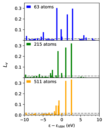
Figure 1: Localization factor ($L_{V}$, see Eq. 30) as a function of the energy of the Kohn-Sham orbitals, relative to the energy of the valence band maximum (VBM), for a NV- center in diamond. We present results for supercells of three different sizes. The threshold used to define the active space is 5% (see text).

4.2 Negatively-charged nitrogen vacancy center in diamond

As a prototypical spin qubit for quantum information science^{56, 57, 58}, the NV- center in diamond has been extensively studied on different levels of theory^{59, 60, 61, 39, 36, 40}. It is generally recognized ^{62, 63} that the four dangling bonds around the defect form a minimal model for the active space, with two non-degenerate $a_{1}$ orbitals, and two degenerate orbitals with $e$ character.

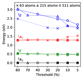
Figure 2: Computed vertical excitation energies of the NV- center in diamond as a function of the chosen threshold of the localization factor $L_{V}$ (see Eq. 30). States are labeled using the irreducible representation of the $C_{3v}$ point group. We present results obtained with the PBE functional for cells of three different sizes. We note that 80% corresponds to a (4o, 6e), (3o, 4e) or (3o, 4e) active space for a 63-, 215- or 511-atom supercell respectively, and 5% corresponds to a (22o, 42e), (14o, 26e) or (12o, 22e) active space for a 63-, 215- or 511-atom supercell respectively.

Instead of constructing a model with a priori knowledge of the defect electronic structure, we determine the active-space composition and size with the help of the localization factor defined in Eq. 30, as shown in Fig. 1. When using 63-, 215- and 511-atom supercells, irrespective of the threshold used to define $L_{V}$, we find three defect orbitals with energies within the band gap of diamond, corresponding to the two degenerate $e$ orbitals and to one of the $a_{1}$ orbital of the minimal model. In the 63- and 215-atom supercells, we find that one of the $a_{1}$ orbitals belonging to the minimal model is below the VBM of diamond; in the 511-atom cell we find instead that three localized orbitals are below the VBM, indicating that at least 6 orbitals are required to define the active space. This suggests that the minimal model with a fixed number of orbitals may be insufficient to accurately describe the system with a large supercell.

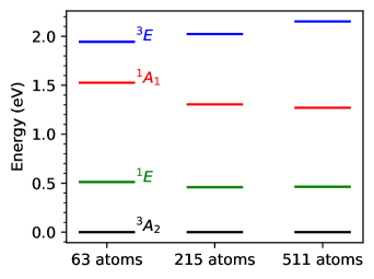
Figure 3: Computed vertical excitation energies for the NV- in diamond. We show converged results (see Fig. 2) at 5% localization threshold as a function of the supercell size, obtained with the PBE functional.

In Fig. 2 we show the vertical excitation energies of the NV- center obtained by diagonalizing the effective Hamiltonian (Eq. 1), as a function of the localization threshold chosen to define $L_{V}$. Irrespective of the chosen threshold, we find that the ground state has ${}^{3}A_{1}$ symmetry. We also find that the lowest excited states with ${}^{1}E$ and ${}^{1}A_{1}$ symmetry converge much faster as a function of the $L_{V}$ threshold than ${}^{3}E$, since ${}^{3}E$ arises from $a_{1}^{1}e^{3}$ configurations rather than a $a_{1}^{2}e^{2}$ configurations, as in the case of ${}^{3}A_{2}$, ${}^{1}E$ and ${}^{1}A_{1}$. Most orbitals added to the active space when decreasing the localization threshold exhibit $a_{1}$ character. We note that the convergence of the ${}^{1}A_{1}$ state in the 63-atom cell is not smooth, probably due to orbitals with $e$ character being part of the active space as the threshold value is decreased. Overall our results point at the need to converge the composition and size of the active space both as a function of $L_{V}$ and cell size. In Fig. 3 we show the vertical excitation energies of the NV- center as a function of supercell size, and the values are summarized in Tab. 1. We chose a 5% $L_{V}$ threshold, i.e. all orbitals with $L_{V}\geq 0.05$ are included in the active space $A$. As shown in Tab. 1, results obtained using the EDC@$G_{0}W_{0}$ correction are much closer to the experimental values than those computed using the original Hartree-Fock double counting correction (see Section 2.2.3), which we call here HFDC. Furthermore, we find unphysical excitations (i.e. states that do not have any experimental counterpart) with HFDC; however such unphysical states are not present when we use the EDC@$G_{0}W_{0}$ correction (see Sec. 7.3 of the SI for details).

In our previous work, using HFDC corrrections we found substantial differences between results obtained with the PBE or the hybrid functional DDH^{53, 64, 65, 66, 67, 68}. Hence we analyze the influence of the chosen functional when using the EDC@$G_{0}W_{0}$ correction. In Fig. 4 and 5, we compare PBE and DDH results for the NV- center, for converged active space in a 215-atom cell. Our results indicate that, except for a widening of the bandgap, the electronic structure is almost insensitive to the choice of the functional. The order of localized defect states within the gap and their localization properties are nearly identical when using PBE and DDH, and the shift of the position of the defect orbitals relative to the band edges is mostly due to the difference in the PBE and DDH bandgaps. The excitation energies of DDH calculations are less than 0.1 eV higher than their PBE counterparts. It is reasonable to expect that the insensitivity to the functional found here in the case of the NV- center may apply more generally to other classes of covalently bonded semiconductors; it appears that the sensitivity observed with the HFDC scheme may have been caused by the incomplete double counting correction of the DFT exchange-correlation effects. However obtaining results for additional defects and solids will be necessary to come to a firm conclusion.

Table 1: Computed vertical excitation energies (eV) for the NV- in diamond for three states (see Fig. 3) obtained with QDET, the PBE functional and 511-atom supercells. We show results using the Hartree-Fock double counting (HFDC) and exact double counting (EDC@$G_{0}W_{0}$) schemes (see text). We also report experimental results (Exp), including results for zero-phonon lines (ZPL), and results obtained using $GW$ and the Bethe-Salpeter Equation (BSE), model fit from $GW$ solved by configuration interaction (CI), model obtained from constrained random phase approximation (cRPA) solved by CI, and quantum chemistry results on clusters from complete active space self-consistent field (CASSCF), multireference configuration interaction (MRCI) and Monte Carlo configuration interaction (MCCI).

Reference$\backslash$Electronic States	${}^{1}E$	${}^{1}A_{1}$	${}^{3}E$
Exp56			2.18
Exp ZPL56, 57, 69, 58, 70	0.34–0.43	1.51–1.60	1.945
QDET (EDC@$G_{0}W_{0}$)	0.463	1.270	2.152
QDET (HFDC)	0.375	1.150	1.324
$GW$ + BSE71	0.40	0.99	2.32
Model fit from $GW$ + CI61	0.5	1.5	2.1
Model from CRPA + CI39	0.49	1.41	2.02
C_85 H_76 N^- CASSCF(6,6)72	0.25	1.60	2.14
C_49 H_52 N^- CASSCF(6,8)73			2.57
C_19 H_28 N^- MRCI(8,10)74	0.50	1.23	1.36
C_42 H_42 N^- MCCI75	0.63	2.06	1.96

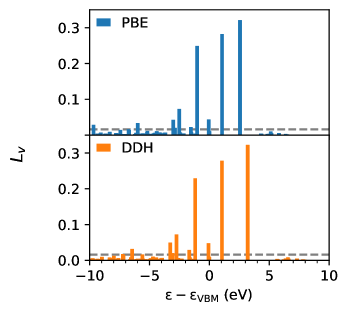
Figure 4: Localization factor ($L_{V}$, see Eq. 30) as a function of the energy of the Kohn-Sham orbitals, relative to the energy of the valence band maximum (VBM), for a NV- center in diamond. We present results for 215-atom cell obtained with the PBE and DDH functionals. The threshold used to define the active space is 5% (see text).

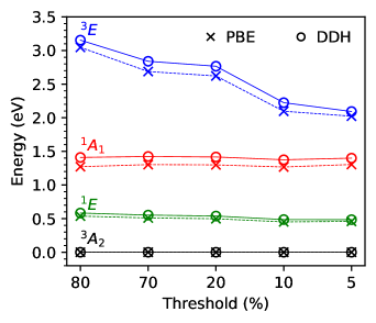
Figure 5: Computed vertical excitation energies of the NV- center in diamond as a function of the chosen threshold of the localization factor $L_{V}$ (see Eq. 30) to define the active space. States are labeled using the irreducible representation of the $C_{3v}$ point group. We present results for 215-atom cell obtained with the PBE and DDH functionals. We note that 80% threshold corresponds to a (3o, 4e) active space, and 5% threshold corresponds to a (14o, 26e) or (15o, 28e) active space for PBE or DDH respectively.

4.3 Neutral group-IV vacancy centers in diamond

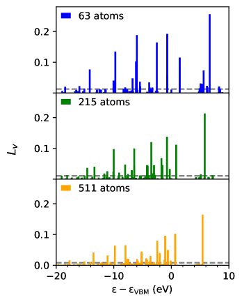
Figure 6: Localization factor ($L_{V}$, see Eq. 30) as a function of the energy of the Kohn-Sham orbitals, relative to the energy of the valence band maximum (VBM), for a SiV^0 center in diamond. We present results for supercells of three different sizes. The threshold used to define the active space is 5% (see text).

In the last decade, a number of studies have investigated group-IV vacancy centers in diamond^{76, 77, 78, 79, 80, 36, 40}, using either a four-orbital⁷⁹ or a nine-orbital minimal model⁴⁰.

Similar to the case of the NV- in diamond, we determine the active space using the localization factor shown in Fig. 6. We find a considerable number of localized orbitals. We exclude from the active space the localized conduction band orbitals, which are around 5 eV in SiV^0, since we found their contribution to the excitation energies to be negligible (see Sec. 6 of the SI). We also exclude the defect atom’s strongly-bound atomic orbitals, present at about -20 eV in GeV^0, SnV^0 and PbV^0, which have almost no hybridization with the host orbitals.

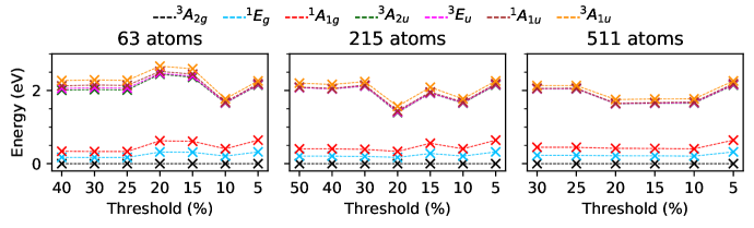
Figure 7: Computed vertical excitation energies of the SiV^0 center in diamond as a function of the chosen threshold of the localization factor $L_{V}$ (see Eq. 30) to define the active space. States are labeled using the irreducible representation of the $D_{3d}$ point group. We present results obtained with the PBE functional for cells of three different sizes. We note that a 40%, 50% or 30% threshold corresponds to a (7o, 12e), (5o, 8e) or (9o, 16e) active space for a 63-, 215- or 511-atom supercell respectively, and 5% threshold corresponds to a (32o, 62e), (40o, 78e) or (48o, 94e) active space for a 63-, 215- or 511-atom supercell respectively.

The vertical excitation energies of SiV^0 as a function of the localization threshold is reported in Fig. 7. In all three supercells we find a slow convergence of the excitation energies, indicating that the excited states of this system are the result of the combination of many single-particle orbitals, and that a minimal model may be insufficient to obtain reliable excitation energies. Using the converged excitation energies for a given supercell, we show the convergence with supercell size in Fig. 8. Similar to the case of the NV^- center, the low-energy excitations are well converged with a 63-atom supercell, while the convergence of the ${}^{3}A_{2u}$, ${}^{3}E_{u}$, ${}^{1}A_{1u}$, and ${}^{3}A_{1u}$ states is slower. In Tab. 2, we compare our best converged values obtained with the EDC@$G_{0}W_{0}$ correction with those obtained with the HFDC correction, as well as with available experimental and theoretical data. In general, the energies predicted using EDC@$G_{0}W_{0}$ are higher than those obtained with HFDC, and in better agreement with those of quantum chemical cluster calculations³⁸. We note that the experimental zero phonon line (ZPL) corresponding to the ${}^{3}E_{u}$ level is 1.31 eV, but the contribution from the dynamical Jahn-Teller effect is unknown. Furthermore, the excitation energies computed with EDC@$G_{0}W_{0}$ show faster convergence compared to those with HFDC. For example, using EDC@$G_{0}W_{0}$ (HFDC) we find a difference of 0.15 (0.65) eV with 63-atom and 215-atom cells. As shown in Figs. 9 and 10, our results with the EDC@$G_{0}W_{0}$ scheme showed insensitivity to the choice of the functional. Our results for GeV^0, SnV^0 and PbV^0 are similar to those of SiV^0 and are summarized in Tab. 2 as well as Tab. S1 in the SI.

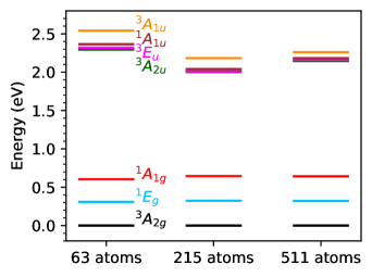
Figure 8: Computed vertical excitation energies for the SiV^0 in diamond. We show converged results (see Fig. 2) at 5% localization threshold, as a function of the supercell size, obtained with the PBE functional.

Table 2: Computed vertical excitation energies (eV) for the SiV^0, GeV^0, SnV^0 and PbV^0 in diamond for six states (see also Fig. 8 for the SiV^0 results) obtained with QDET, the PBE functional and 511-atom supercells. We show results using the Hartree-Fock double counting (HFDC) and exact double counting (EDC@$G_{0}W_{0}$) schemes (see text). We also report experimental results for zero-phonon lines (ZPL), and results obtained with a combination of second-order $N$-electron valence state perturbation theory (NEVPT2) and density matrix embedding theory (DMET), and quantum chemistry calculations on clusters from NEVPT2.

System	Reference$\backslash$Electronic States	${}^{1}E_{g}$	${}^{1}A_{1g}$	${}^{3}A_{2u}$	${}^{3}E_{u}$	${}^{1}A_{1u}$	${}^{3}A_{1u}$
SiV^0	Exp ZPL				1.31
	QDET (EDC@$G_{0}W_{0}$)	0.321	0.642	2.146	2.161	2.183	2.260
	QDET (HFDC)	0.236	0.435	1.098	1.096	1.111	1.188
	NEVPT2-DMET(10,12)38	0.51	1.14	2.39	2.47		2.61
	C_84 H_78 Si_0 NEVPT2(10,12)38	0.54	1.10	2.10	2.16		2.14
GeV^0	QDET (EDC@$G_{0}W_{0}$)	0.357	0.717	2.924	2.925	2.940	2.970
	QDET (HFDC)	0.289	0.554	1.456	1.443	1.443	1.495
SnV^0	QDET (EDC@$G_{0}W_{0}$)	0.295	0.596	2.590	2.571	2.561	2.616
	QDET (HFDC)	0.276	0.551	1.459	1.444	1.436	1.491
PbV^0	QDET (EDC@$G_{0}W_{0}$)	0.319	0.640	3.095	3.072	3.056	3.099
	QDET (HFDC)	0.302	0.600	1.788	1.768	1.755	1.796

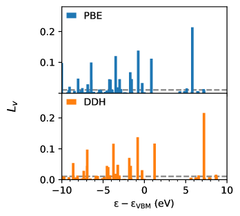
Figure 9: Localization factor ($L_{V}$, see Eq. 30) as a function of the energy of the Kohn-Sham orbitals, relative to the energy of the valence band maximum (VBM), for a SiV^0 center in diamond. We present results for a 215-atom cell obtained with the PBE and DDH functionals. The threshold used to define the active space is 5% (see text).

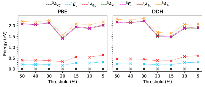
Figure 10: Computed vertical excitation energies (eV) of the NV- center in diamond as a function of the chosen threshold of the localization factor $L_{V}$ (see Eq. 30). States are labeled using the irreducible representation of the $D_{3d}$ point group. We present results for a 215-atom cell obtained with the PBE and DDH functionals.

5 Conclusions

In summary, in this work we presented a Green’s function formulation of the quantum defect embedding theory (QDET) that enables the definition of an improved correction to the double counting scheme originally adopted in Refs 36, 37. We defined an effective Hamiltonian for the active space within a Green’s function formalism, where the effective interaction is static and the self-energy cross-terms between the active space and the environment are neglected. Our results show that these approximations are appropriate to describe the localized defect states in semiconductors investigated in this work. Within the Green’s function formalism adopted here, we derived an exact double counting scheme (EDC@$G_{0}W_{0}$) replacing the approximate scheme originally adopted in Refs 36, 37. We emphasize that the double counting correction EDC@$G_{0}W_{0}$ enables the removal of any double counting terms arising from the separation of the whole system into active space and environment. We then described the implementation of the scheme within the WEST code ⁴³, including a strategy to ensure convergence of our calculations with respect to the size and composition of the active space. Further, we demonstrated that QDET with exact double counting provides reliable results for several defects in diamond, with negligible dependence on the functional chosen for the underlying DFT calculations of the defects. Work is in progress to apply QDET with the EDC@$G_{0}W_{0}$ scheme to more complex systems, such as defects in oxides and molecules on surfaces.

Supporting information

Definition of matrix elements (section 1), comparison with other double counting schemes in the literature (section 2), implementation details (section 3), Hartree-Fock double counting (section 4), convergence of QDET calculations (section 5), discussion of ghost states (section 6), and a table of vertical excitation energies (section 7).

References

- Hohenberg and Kohn 1964 Hohenberg, P.; Kohn, W. Inhomogeneous Electron Gas. Phys. Rev. 1964, 136, B864–B871
- Kohn and Sham 1965 Kohn, W.; Sham, L. J. Self-Consistent Equations Including Exchange and Correlation Effects. Phys. Rev. 1965, 140, A1133–A1138
- Neugebauer and Hickel 2013 Neugebauer, J.; Hickel, T. Density Functional Theory in Materials Science. WIREs Computational Molecular Science 2013, 3, 438–448
- Mardirossian and Head-Gordon 2017 Mardirossian, N.; Head-Gordon, M. Thirty Years of Density Functional Theory in Computational Chemistry: An Overview and Extensive Assessment of 200 Density Functionals. Mol. Phys. 2017, 115, 2315–2372
- Jones 2015 Jones, R. O. Density Functional Theory: Its Origins, Rise to Prominence, and Future. Rev. Mod. Phys. 2015, 87, 897–923
- Burke 2012 Burke, K. Perspective on density functional theory. J. Chem. Phys. 2012, 136, 150901
- Strinati 1988 Strinati, G. Application of the green’s functions method to the study of the optical properties of semiconductors. Riv. Nuovo Cimento 1988, 11, 1–86
- Martin et al. 2016 Martin, R. M.; Reining, L.; Ceperley, D. M. Interacting electrons; Cambridge University Press, 2016
- Golze et al. 2019 Golze, D.; Dvorak, M.; Rinke, P. The GW Compendium: A Practical Guide to Theoretical Photoemission Spectroscopy. Front. Chem. 2019, 7, 377
- Bartlett and Musiał 2007 Bartlett, R. J.; Musiał, M. Coupled-Cluster Theory in Quantum Chemistry. Rev. Mod. Phys. 2007, 79, 291–352
- Zhang and Grüneis 2019 Zhang, I. Y.; Grüneis, A. Coupled Cluster Theory in Materials Science. Front. Mater. 2019, 6
- Helgaker et al. 2014 Helgaker, T.; Jorgensen, P.; Olsen, J. Molecular electronic-structure theory; John Wiley & Sons, 2014
- Sun and Chan 2016 Sun, Q.; Chan, G. K.-L. Quantum Embedding Theories. Acc. Chem. Res. 2016, 49, 2705–2712
- Jones et al. 2020 Jones, L. O.; Mosquera, M. A.; Schatz, G. C.; Ratner, M. A. Embedding Methods for Quantum Chemistry: Applications from Materials to Life Sciences. J. Am. Chem. Soc. 2020, 142, 3281–3295
- Sheng et al. 2021 Sheng, N.; Vorwerk, C.; Govoni, M.; Galli, G. Quantum Simulations of Material Properties on Quantum Computers. arXiv:2105.04736 [cond-mat, physics:quant-ph] 2021, arXiv: 2105.04736
- Senn and Thiel 2009 Senn, H. M.; Thiel, W. QM/MM Methods for Biomolecular Systems. Angew. Chem. Int. Ed. 2009, 48, 1198–1229
- Liu et al. 2014 Liu, M.; Wang, Y.; Chen, Y.; Field, M. J.; Gao, J. QM/MM through the 1990s: The First Twenty Years of Method Development and Applications. Isr. J. Chem. 2014, 54, 1250–1263
- Libisch et al. 2014 Libisch, F.; Huang, C.; Carter, E. A. Embedded Correlated Wavefunction Schemes: Theory and Applications. Acc. Chem. Res. 2014, 47, 2768–2775
- Gomes et al. 2008 Gomes, A. S. P.; Jacob, C. R.; Visscher, L. Calculation of Local Excitations in Large Systems by Embedding Wave-Function Theory in Density-Functional Theory. Phys. Chem. Chem. Phys. 2008, 10, 5353–5362
- Goodpaster et al. 2012 Goodpaster, J. D.; Barnes, T. A.; Manby, F. R.; Miller, T. F. Density Functional Theory Embedding for Correlated Wavefunctions: Improved Methods for Open-Shell Systems and Transition Metal Complexes. J. Chem. Phys. 2012, 137, 224113
- Wouters et al. 2016 Wouters, S.; Jiménez-Hoyos, C. A.; Sun, Q.; Chan, G. K.-L. A Practical Guide to Density Matrix Embedding Theory in Quantum Chemistry. J. Chem. Theory. Comput. 2016, 12, 2706–2719
- Knizia and Chan 2012 Knizia, G.; Chan, G. K.-L. Density Matrix Embedding: A Simple Alternative to Dynamical Mean-Field Theory. Phys. Rev. Lett. 2012, 109, 186404
- Knizia and Chan 2013 Knizia, G.; Chan, G. K.-L. Density Matrix Embedding: A Strong-Coupling Quantum Embedding Theory. J. Chem. Theory. Comput. 2013, 9, 1428–1432
- Cui et al. 2020 Cui, Z.-H.; Zhu, T.; Chan, G. K.-L. Efficient Implementation of Ab Initio Quantum Embedding in Periodic Systems: Density Matrix Embedding Theory. 2020, 16, 119–129
- Pham et al. 2020 Pham, H. Q.; Hermes, M. R.; Gagliardi, L. Periodic Electronic Structure Calculations with the Density Matrix Embedding Theory. J. Chem. Theory. Comput. 2020, 16, 130–140
- Hermes and Gagliardi 2019 Hermes, M. R.; Gagliardi, L. Multiconfigurational Self-Consistent Field Theory with Density Matrix Embedding: The Localized Active Space Self-Consistent Field Method. J. Chem. Theory. Comput. 2019, 15, 972–986
- Pham et al. 2018 Pham, H. Q.; Bernales, V.; Gagliardi, L. Can Density Matrix Embedding Theory with the Complete Activate Space Self-Consistent Field Solver Describe Single and Double Bond Breaking in Molecular Systems? J. Chem. Theory. Comput. 2018, 14, 1960–1968
- Lan and Zgid 2017 Lan, T. N.; Zgid, D. Generalized Self-Energy Embedding Theory. J. Chem. Phys. Lett. 2017, 8, 2200–2205
- Zgid and Gull 2017 Zgid, D.; Gull, E. Finite Temperature Quantum Embedding Theories for Correlated Systems. New. J. Phys. 2017, 19, 023047
- Rusakov et al. 2019 Rusakov, A. A.; Iskakov, S.; Tran, L. N.; Zgid, D. Self-Energy Embedding Theory (SEET) for Periodic Systems. J. Chem. Theory. Comput. 2019, 15, 229–240
- Georges and Kotliar 1992 Georges, A.; Kotliar, G. Hubbard Model in Infinite Dimensions. Phys. Rev. B 1992, 45, 6479–6483
- Georges et al. 1996 Georges, A.; Kotliar, G.; Krauth, W.; Rozenberg, M. J. Dynamical Mean-Field Theory of Strongly Correlated Fermion Systems and the Limit of Infinite Dimensions. Rev. Mod. Phys. 1996, 68, 13–125
- Georges 2004 Georges, A. Strongly Correlated Electron Materials: Dynamical Mean-Field Theory and Electronic Structure. AIP Conf. Proc. 2004, 715, 3–74
- Anisimov et al. 1997 Anisimov, V. I.; Poteryaev, A. I.; Korotin, M. A.; Anokhin, A. O.; Kotliar, G. First-Principles Calculations of the Electronic Structure and Spectra of Strongly Correlated Systems: Dynamical Mean-Field Theory. J. Phys. Condens. Matter. 1997, 9, 7359–7367
- Kotliar et al. 2006 Kotliar, G.; Savrasov, S. Y.; Haule, K.; Oudovenko, V. S.; Parcollet, O.; Marianetti, C. A. Electronic Structure Calculations with Dynamical Mean-Field Theory. Rev. Mod. Phys. 2006, 78, 865–951
- Ma et al. 2020 Ma, H.; Govoni, M.; Galli, G. Quantum Simulations of Materials on Near-Term Quantum Computers. npj Comput. Mater. 2020, 6, 1–8
- Ma et al. 2021 Ma, H.; Sheng, N.; Govoni, M.; Galli, G. Quantum Embedding Theory for Strongly Correlated States in Materials. J. Chem. Theory. Comput. 2021, 17, 2116–2125
- Mitra et al. 2021 Mitra, A.; Pham, H. Q.; Pandharkar, R.; Hermes, M. R.; Gagliardi, L. Excited States of Crystalline Point Defects with Multireference Density Matrix Embedding Theory. J. Phys. Chem. Lett. 2021, 12, 11688–11694
- Bockstedte et al. 2018 Bockstedte, M.; Schütz, F.; Garratt, T.; Ivády, V.; Gali, A. Ab initio description of highly correlated states in defects for realizing quantum bits. npj Quantum Mater. 2018, 3, 1–6
- Ma et al. 2020 Ma, H.; Sheng, N.; Govoni, M.; Galli, G. First-Principles Studies of Strongly Correlated States in Defect Spin Qubits in Diamond. Phys. Chem. Chem. Phys. 2020, 22, 25522–25527
- Muechler et al. 2021 Muechler, L.; Badrtdinov, D. I.; Hampel, A.; Cano, J.; Rösner, M.; Dreyer, C. E. Quantum embedding methods for correlated excited states of point defects: Case studies and challenges. arXiv:2105.08705 [cond-mat] 2021, arXiv: 2105.08705
- Pfäffle et al. 2021 Pfäffle, W.; Antonov, D.; Wrachtrup, J.; Bester, G. Screened configuration interaction method for open-shell excited states applied to NV centers. Phys. Rev. B 2021, 104, 104105
- Govoni and Galli 2015 Govoni, M.; Galli, G. Large Scale GW Calculations. J. Chem. Theory. Comput. 2015, 11, 2680–2696
- Wilson et al. 2008 Wilson, H. F.; Gygi, F.; Galli, G. Efficient iterative method for calculations of dielectric matrices. Phys. Rev. B 2008, 78, 113303
- Baroni et al. 2001 Baroni, S.; de Gironcoli, S.; Dal Corso, A.; Giannozzi, P. Phonons and Related Crystal Properties from Density-Functional Perturbation Theory. Rev. Mod. Phys. 2001, 73, 515–562
- Umari et al. 2010 Umari, P.; Stenuit, G.; Baroni, S. GW quasiparticle spectra from occupied states only. Phys. Rev. B 2010, 81, 115104
- Nguyen et al. 2012 Nguyen, H.-V.; Pham, T. A.; Rocca, D.; Galli, G. Improving Accuracy and Efficiency of Calculations of Photoemission Spectra within the Many-Body Perturbation Theory. Phys. Rev. B 2012, 85, 081101
- Godby et al. 1988 Godby, R. W.; Schlüter, M.; Sham, L. J. Self-Energy Operators and Exchange-Correlation Potentials in Semiconductors. Phys. Rev. B 1988, 37, 10159–10175
- Giantomassi et al. 2011 Giantomassi, M.; Stankovski, M.; Shaltaf, R.; Grüning, M.; Bruneval, F.; Rinke, P.; Rignanese, G.-M. Electronic Properties of Interfaces and Defects from Many-Body Perturbation Theory: Recent Developments and Applications. Phys. Status Solidi B 2011, 248, 275–289
- van Schilfgaarde et al. 2006 van Schilfgaarde, M.; Kotani, T.; Faleev, S. Quasiparticle Self-Consistent G W Theory. Phys. Rev. Lett. 2006, 96, 226402
- Giannozzi et al. 2009 Giannozzi, P.; Baroni, S.; Bonini, N.; Calandra, M.; Car, R.; Cavazzoni, C.; Ceresoli, D.; Chiarotti, G. L.; Cococcioni, M.; Dabo, I.; Corso, A. D.; de Gironcoli, S.; Fabris, S.; Fratesi, G.; Gebauer, R.; Gerstmann, U.; Gougoussis, C.; Kokalj, A.; Lazzeri, M.; Martin-Samos, L.; Marzari, N.; Mauri, F.; Mazzarello, R.; Paolini, S.; Pasquarello, A.; Paulatto, L.; Sbraccia, C.; Scandolo, S.; Sclauzero, G.; Seitsonen, A. P.; Smogunov, A.; Umari, P.; Wentzcovitch, R. M. QUANTUM ESPRESSO: a modular and open-source software project for quantum simulations of materials. J. Phys.: Condens. Matter 2009, 21, 395502
- Perdew et al. 1996 Perdew, J. P.; Burke, K.; Ernzerhof, M. Generalized Gradient Approximation Made Simple. Phys. Rev. Lett. 1996, 77, 3865–3868
- Skone et al. 2014 Skone, J. H.; Govoni, M.; Galli, G. Self-consistent hybrid functional for condensed systems. Phys. Rev. B 2014, 89, 195112
- Schlipf and Gygi 2015 Schlipf, M.; Gygi, F. Optimization algorithm for the generation of ONCV pseudopotentials. Comput. Phys. Commun. 2015, 196, 36–44
- Sun et al. 2018 Sun, Q.; Berkelbach, T. C.; Blunt, N. S.; Booth, G. H.; Guo, S.; Li, Z.; Liu, J.; McClain, J. D.; Sayfutyarova, E. R.; Sharma, S.; Wouters, S.; Chan, G. K.-L. PySCF: The Python-Based Simulations of Chemistry Framework. WIREs Comput. Mol. Sci. 2018, 8, e1340
- Davies et al. 1976 Davies, G.; Hamer, M. F.; Price, W. C. Optical Studies of the 1.945 eV Vibronic Band in Diamond. Proc. R. Soc. London A 1976, 348, 285–298
- Rogers et al. 2008 Rogers, L. J.; Armstrong, S.; Sellars, M. J.; Manson, N. B. Infrared emission of the NV centre in diamond: Zeeman and uniaxial stress studies. New J. Phys. 2008, 10, 103024
- Goldman et al. 2015 Goldman, M. L.; Sipahigil, A.; Doherty, M. W.; Yao, N. Y.; Bennett, S. D.; Markham, M.; Twitchen, D. J.; Manson, N. B.; Kubanek, A.; Lukin, M. D. Phonon-Induced Population Dynamics and Intersystem Crossing in Nitrogen-Vacancy Centers. Phys. Rev. Lett. 2015, 114, 145502
- Doherty et al. 2011 Doherty, M. W.; Manson, N. B.; Delaney, P.; Hollenberg, L. C. L. The negatively charged nitrogen-vacancy centre in diamond: the electronic solution. New J. Phys. 2011, 13, 025019
- Maze et al. 2011 Maze, J. R.; Gali, A.; Togan, E.; Chu, Y.; Trifonov, A.; Kaxiras, E.; Lukin, M. D. Properties of nitrogen-vacancy centers in diamond: the group theoretic approach. New J. Phys. 2011, 13, 025025
- Choi et al. 2012 Choi, S.; Jain, M.; Louie, S. G. Mechanism for optical initialization of spin in NV-center in diamond. Phys. Rev. B 2012, 86, 041202
- Loubser and van Wyk 1978 Loubser, J. H. N.; van Wyk, J. A. Electron Spin Resonance in the Study of Diamond. Rep. Prog. Phys. 1978, 41, 1201–1248
- Doherty et al. 2013 Doherty, M. W.; Manson, N. B.; Delaney, P.; Jelezko, F.; Wrachtrup, J.; Hollenberg, L. C. The nitrogen-vacancy colour centre in diamond. Phys. Rep. 2013, 528, 1–45
- Skone et al. 2016 Skone, J. H.; Govoni, M.; Galli, G. Nonempirical range-separated hybrid functionals for solids and molecules. Phys. Rev. B 2016, 93, 235106
- Brawand et al. 2016 Brawand, N. P.; Vörös, M.; Govoni, M.; Galli, G. Generalization of Dielectric-Dependent Hybrid Functionals to Finite Systems. Phys. Rev. X 2016, 6, 041002
- Brawand et al. 2017 Brawand, N. P.; Govoni, M.; Vörös, M.; Galli, G. Performance and Self-Consistency of the Generalized Dielectric Dependent Hybrid Functional. J. Chem. Theory Comput. 2017, 13, 3318–3325, PMID: 28537727
- Gerosa et al. 2017 Gerosa, M.; Bottani, C. E.; Valentin, C. D.; Onida, G.; Pacchioni, G. Accuracy of dielectric-dependent hybrid functionals in the prediction of optoelectronic properties of metal oxide semiconductors: a comprehensive comparison with many-body GW and experiments. J. Phys.: Condens. Matter 2017, 30, 044003
- Zheng et al. 2019 Zheng, H.; Govoni, M.; Galli, G. Dielectric-dependent hybrid functionals for heterogeneous materials. Phys. Rev. Materials 2019, 3, 073803
- Kehayias et al. 2013 Kehayias, P.; Doherty, M. W.; English, D.; Fischer, R.; Jarmola, A.; Jensen, K.; Leefer, N.; Hemmer, P.; Manson, N. B.; Budker, D. Infrared Absorption Band and Vibronic Structure of the Nitrogen-Vacancy Center in Diamond. Phys. Rev. B 2013, 88, 165202
- Goldman et al. 2015 Goldman, M. L.; Doherty, M. W.; Sipahigil, A.; Yao, N. Y.; Bennett, S. D.; Manson, N. B.; Kubanek, A.; Lukin, M. D. State-Selective Intersystem Crossing in Nitrogen-Vacancy Centers. Phys. Rev. B 2015, 91, 165201
- Ma et al. 2010 Ma, Y.; Rohlfing, M.; Gali, A. Excited States of the Negatively Charged Nitrogen-Vacancy Color Center in Diamond. Phys. Rev. B 2010, 81, 041204
- Bhandari et al. 2021 Bhandari, C.; Wysocki, A. L.; Economou, S. E.; Dev, P.; Park, K. Multiconfigurational Study of the Negatively Charged Nitrogen-Vacancy Center in Diamond. Phys. Rev. B 2021, 103, 014115
- Lin et al. 2008 Lin, C.-K.; Wang, Y.-H.; Chang, H.-C.; Hayashi, M.; Lin, S. H. One- and Two-Photon Absorption Properties of Diamond Nitrogen-Vacancy Defect Centers: A Theoretical Study. J. Chem. Phys. 2008, 129, 124714
- Zyubin et al. 2009 Zyubin, A. S.; Mebel, A. M.; Hayashi, M.; Chang, H. C.; Lin, S. H. Quantum Chemical Modeling of Photoadsorption Properties of the Nitrogen-Vacancy Point Defect in Diamond. J. Comput. Chem. 2009, 30, 119–131
- Delaney et al. 2010 Delaney, P.; Greer, J. C.; Larsson, J. A. Spin-Polarization Mechanisms of the Nitrogen-Vacancy Center in Diamond. Nano Lett. 2010, 10, 610–614
- Gali and Maze 2013 Gali, A.; Maze, J. R. Ab initio study of the split silicon-vacancy defect in diamond: Electronic structure and related properties. Phys. Rev. B 2013, 88, 235205
- Thiering and Gali 2018 Thiering, G. m. H.; Gali, A. Ab Initio Magneto-Optical Spectrum of Group-IV Vacancy Color Centers in Diamond. Phys. Rev. X 2018, 8, 021063
- Green et al. 2019 Green, B. L.; Doherty, M. W.; Nako, E.; Manson, N. B.; D’Haenens-Johansson, U. F. S.; Williams, S. D.; Twitchen, D. J.; Newton, M. E. Electronic Structure of the Neutral Silicon-Vacancy Center in Diamond. Phys. Rev. B 2019, 99, 161112
- Thiering and Gali 2019 Thiering, G.; Gali, A. The (eg eu) Eg product Jahn–Teller effect in the neutral group-IV vacancy quantum bits in diamond. npj Comput. Mater. 2019, 5, 18
- Zhang et al. 2020 Zhang, Z.-H.; Stevenson, P.; Thiering, G.; Rose, B. C.; Huang, D.; Edmonds, A. M.; Markham, M. L.; Lyon, S. A.; Gali, A.; de Leon, N. P. Optically Detected Magnetic Resonance in Neutral Silicon Vacancy Centers in Diamond via Bound Exciton States. Phys. Rev. Lett. 2020, 125, 237402