Error mitigation increases the effective quantum volume of quantum computers

Abstract

Quantum volume is a single-number metric which, loosely speaking, reports the number of usable qubits on a quantum computer. While improvements to the underlying hardware are a direct means of increasing quantum volume, the metric is “full-stack” and has also been increased by improvements to software, notably compilers. We extend this latter direction by demonstrating that error mitigation, a type of indirect compilation, increases the effective quantum volume of several quantum computers. Importantly, this increase occurs while taking the same number of overall samples. We encourage the adoption of quantum volume as a benchmark for assessing the performance of error mitigation techniques.

Introduction   Quantum volume [1] is a single-number metric which, loosely speaking, reports the number of usable qubits on a quantum computer. While improvements to the underlying hardware are a direct means of increasing quantum volume, the metric is “full-stack” and can be increased by an improvement to any component, e.g. software for compilation to produce an equivalent quantum circuit with fewer elementary operations [2].

Given an $m$ qubit quantum circuit $C$, the heavy set is $\mathcal{H}_{C}:=\{z\in\{0,1\}^{m}:p(z)>p_{\text{median}}\}$ where $p(z):=\left|\langle z|C|0\rangle\right|^{2}$ is the probability of sampling bitstring $z$ and $p_{\text{median}}$ is the median probability over all bitstrings. A heavy bitstring is one in the heavy set. Quantum volume is determined by counting the number of heavy bitstrings $n_{h}$ measured over $n_{c}$ random circuits, each sampled $n_{s}$ times. If the experiment is run with $m$ qubit circuits of depth $d=m$, $n_{c}\geq 100$, and

$$\hat{h}_{d}:={n_{h}}/{n_{c}n_{s}}>2/3+2\sigma$$ (1)

where $\sigma$ is the standard deviation of the estimate, then the volume is at least $m$. The actual volume is the largest $m$ such that these conditions are true. The particular structure of these random circuits, which we refer to as quantum volume circuits, is defined in [1].

Method   Given a quantum volume circuit $C$, we define the projector on the heavy subspace

$$\Pi_{h,C}:=\sum_{z\in\mathcal{H}_{C}}|z\rangle\langle z|$$ (2)

so that the expected number of heavy bitstrings for this circuit is $n_{h,C}:=n_{s}\langle 0|C^{\dagger}\Pi_{h,C}C|0\rangle$. We use zero-noise extrapolation (ZNE) [3, 4] with $\Pi_{h,C}$ as the observable for each quantum volume circuit $C$ to estimate the noise-free value of $n_{h}:=\sum_{C}n_{h,C}$. This amounts to evaluating $\langle\Pi_{h,C}^{(\lambda)}\rangle$ at several noise-scale factors $\lambda\geq 1$ then using these results to estimate $\langle\Pi_{h,C}^{(0)}\rangle$, i.e., the zero-noise limit of the heavy output probability. In practice, this means compiling the circuit $C$ to a set of circuits $\{C_{\lambda_{i}}\}_{i=1}^{k}$. For fairness with the unmitigated experiment, we use $n_{s}/k$ samples for each $C_{\lambda_{i}}$ so that the total number of samples drawn is equal in the mitigated and unmitigated experiments. The main difference to previous work improving quantum volume by compiling [2] is that we compile a single circuit to a set of circuits, following the pattern of many error mitigation methods (e.g. [4]), in contrast with compilation that does rewrites on a single circuit following algebraic rules or optimized routing.

After executing each $C_{\lambda_{i}}$ to obtain scaled heavy output counts $n_{h,C}^{(i)}$, we use Richardson extrapolation [4, 5] to estimate the zero-noise result via

$$n_{h,C}^{(0)}=\sum_{i=1}^{k}\eta_{i}n_{h,C}^{(i)}$$ (3)

where coefficients are given by

$$\eta_{i}:=\prod_{j\neq i}\frac{\lambda_{j}}{\lambda_{j}-\lambda_{i}}.$$ (4)

In practice, we use $\lambda_{i}\in\{1,3,5,7,9\}$ and scale circuits by locally folding two-qubit (CNOT) gates [5]. In other words, the scaled circuit for $\lambda_{i}=t$ has each CNOT replaced by $t$ CNOTs.

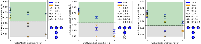
Figure 1: Results of unmitigated and mitigated quantum volume experiments on three five-qubit quantum computers (left-to-right: Belem, Lima, and Quito) using $n_{c}=500$ circuits and $n_{s}=10^{4}$ total samples. Each marker shows the estimated heavy output probability $\hat{h}_{d}$ on a different qubit configuration defined in the legend and error bars show $2\sigma$ intervals evaluated by bootstrapping. The connectivity of each device is shown below each legend. Dashed black lines show the $2/3$ threshold and noiseless asymptote $(1+\ln 2)/2$ [1]. For the mitigated experiments, $\lambda_{i}\in\{1,3,5,7,9\}$ and $n_{s}=10^{4}/5$. Local unitary folding of two-qubit gates is used to compile the circuits (i.e., scale noise) and Richardson’s method of extrapolation is used to infer the zero-noise result. The qubit subsets which achieved the largest quantum volume in the mitigated experiments are colored blue in each device diagram. As can be seen, on Belem error mitigation increases the effective quantum volume from three to five, on Lima error mitigation increases the effective quantum volume from three to four, and on Quito error mitigation increases the effective quantum volume from four to five.

Results   Using this strategy, we perform unmitigated and mitigated quantum volume experiments on the Belem, Lima, and Quito devices available through IBM [6] (see Appendix A for device specifications). The results, shown in Fig. 1, demonstrate that we are able to increase the effective quantum volume from three to five on Belem, three to four on Lima, and from four to five on Quito. Note that ZNE increases the estimated heavy output probability $\hat{h}_{d}$ on all qubit subsets even though the $2/3$ threshold is not always crossed. We therefore expect that ZNE can increase effective quantum volume independent of the size of the device, so long as cross-talk and other errors do not scale with the device size. The largest ZNE experiment to date was performed on $26$ qubit circuits with $1080$ two-qubit gates [7] and, in the context of our work, provides evidence that error mitigation can continue to increase the effective volume of larger quantum devices, e.g. those listed in Appendix B.

Because we estimate the noiseless result by taking a linear combination of noisy results, the way we compute $\sigma$ in (1) changes relative to [1]. For any technique, such as Richardson extrapolation, that evaluates an error-mitigated expectation value as a linear combination of noisy expectation values (3), one can show (see Appendix C) that

$$\sigma^{2}=\frac{1}{n_{c}^{2}}\sum_{C}\sigma_{C}^{2},\qquad \sigma_{C}^{2}=\sum_{i=1}^{k}|\eta_{i}|^{2}(\sigma^{(i)}_{C})^{2},$$ (5)

where $(\sigma^{(i)}_{C})^{2}$ is the variance of each noise-scaled expectation value, while $\sigma_{C}^{2}$ is the variance of the error-mitigated expectation value associated to the quantum circuit $C$. The previous expressions correspond to a theoretical estimate of the error, but in practice we can estimate error bars by repeating the experiment multiple times or by bootstrapping. The $2\sigma$ error bars in Fig. 1 are calculated by bootstrapping with $500$ resamples. See Appendix C for more details.

Discussion   There is a subtle point in interpreting our results in the general context of quantum computer performance. Our error mitigation procedure improves the expectation value of the heavy output projector but does not produce more heavy bitstrings — in fact, our procedure likely produces fewer heavy bitstrings because we distribute samples across circuits at amplified noise levels. However, as we have shown, we are able to use this information to estimate the expected number of heavy bitstrings in a statistically significant way. To carefully distinguish between the two cases, we refer to our results as increasing the effective quantum volume.

The restriction to evaluating expectation values but not directly sampling bitstrings raises interesting questions about physicality and the role of a quantum computer in a computational procedure. If an algorithm only requires expectation values and we apply the error mitigation procedure used in this work, is it the case that we effectively have access to a quantum computer with a larger quantum volume? These questions are linked to the physical interpretation of error mitigation. One way to interpret ZNE is that we evaluate expectation values with respect to the “extrapolated density matrix”

$$\rho_{0}=\sum_{i}\eta_{i}\rho_{\lambda_{i}}$$ (6)

where $\rho_{\lambda_{i}}$ are the noise-scaled physical states and $\eta_{i}$ are the real coefficients in (3). Clearly we did not physically prepare $\rho_{0}$ in our experiment, but should we restrict the use of a quantum computer to only preparing a single physical state from which we can sample bitstrings? Or do we allow ourselves to “virtually” prepare non-physical but mathematically well-defined states from which we can compute expectation values more accurately? We note that similar questions have been asked in the context of virtual distillation techniques [8, 9] which have been proposed to artificially purify a quantum state or to reduce its effective temperature [10].

Conclusion   In this work we have experimentally demonstrated that error mitigation improves the effective quantum volume of several quantum computers. We use the term effective quantum volume to emphasize that our procedure is appropriate for algorithms computing expectation values and not for algorithms requiring individual bitstrings. The error mitigation technique is not tailored to the structure of quantum volume circuits or to the architecture of the quantum computers we used. Indeed, we did not run any additional calibration experiments or use any calibration information to obtain our results. Similar software-level techniques have been used in previous quantum volume experiments, e.g. (approximate) compilation [1, 2] and dynamical decoupling [2]. The novelty of our proposal is that, by relaxing the strong requirement of directly sampling heavy bitstrings to the weaker requirement of estimating the expectation value of the heavy output projector, more general error mitigation techniques can be applied to improve the effective quantum volume of a device. We expect this approach to improve the effective quantum volume of additional quantum computers such as those in Appendix B. Our open source error mitigation software [11] can be used on many quantum computers to repeat the experiments we performed here.

In the context of error mitigation, our work provides additional benchmarks to the relatively few experimental results in literature [12, 11, 7, 13, 14, 15, 16]. We encourage the use of quantum volume as a benchmark for error mitigation techniques due to its relatively widespread adoption and clear operational meaning. Normalizing by additional resources used (gates, shots, qubits, etc.) in error-mitigated quantum volume experiments provides a way to directly compare different techniques and drive progress in this area. As most error mitigation techniques act on expectation values, they can be used for effective quantum volume experiments as we have done in this work.

Code and data availability The code we used to run experiments as well as the data we collected are available at https://github.com/unitaryfund/mitiq-qv.

Acknowledgements This work was supported by the U.S. Department of Energy, Office of Science, Office of Advanced Scientific Computing Research, Accelerated Research in Quantum Computing under Award Number DE-SC0020266. R.L. acknowledges support from a NASA Space Technology Graduate Research Fellowship. We thank IBM for providing access to their quantum computers and software for reproducing quantum volume experiments. The views expressed in this paper are those of the authors and do not reflect those of IBM.

Appendix A Device specifications

In Table 1 we provide more information about the quantum computers we used in our experiments. Note that the quantum volume of Belem is listed as four at [6] but we are unable to reproduce this result in our unmitigated experiments, presumably due to device degradation over time.

	Lima	Belem	Quito
# Qubits	5	5	5
$\epsilon_{\text{1Q}}$	$4.446\times 10^{-4}$	$2.808\times 10^{-4}$	$2.980\times 10^{-4}$
$\epsilon_{\text{CNOT}}$	$1.131\times 10^{-2}$	$1.098\times 10^{-2}$	$8.292\times 10^{-3}$
$\epsilon_{\text{M}}$	$3.790\times 10^{-2}$	$2.868\times 10^{-2}$	$2.546\times 10^{-2}$

Table 1: Device specifications and error rates for the quantum computers we used in our experiments. Device connectivities are shown in Fig. 1. Parameters $\epsilon_{\text{1Q}}$, $\epsilon_{\text{CX}}$, $\epsilon_{\text{M}}$ denote, respectively, averages (over all qubits) of single-qubit $\sqrt{X}$ gate errors, two-qubit CNOT gate errors, and readout errors $(p(0|1)+p(1|0))/2$ accessed from [6].

Appendix B Table of quantum volumes

As discussed in the main text, error mitigation consistently increased the estimated heavy output probability in all of our experiments. To increment the effective quantum volume of a device, this increase must cross the $2/3$ threshold with statistical significance. While there is no guarantee that this will happen, we expect there to be several cases of already-measured quantum volumes where this will be true. For this reason, as well as general context, we include a list of quantum computer volumes in Table 2.

Quantum computer	$\log\text{QV}$	Reference
Rigetti Aspen-4	3	[17]
Lima	3 (4)	[6] (this work)
Belem	3 (5)	[6] (this work)
Jakarta	4	[6]
Bogota	4	[6]
Quito	4 (5)	[6] (this work)
Manila	5	[6]
Nairobi	5	[6]
Lagos	5	[6]
Perth	5	[6]
Guadalupe	5	[6]
Toronto	5	[6]
Brooklyn	5	[6]
Trapped-ion QCCD	6	[18]
Hanoi	6	[6]
Auckland	6	[6]
Cairo	6	[6]
Washington	6	[6]
Mumbai	7	[6]
Kolkata	7	[6]
Honeywell System Model H1	10	[19]

Table 2: Measured quantum volumes (in increasing order). Values in parentheses show effective quantum volumes measured in this work.

Appendix C Statistical uncertainty of error-mitigated volume

C.1 Theoretical estimation of error bars

For a large number of error mitigation techniques, including Richardson extrapolation, an error-mitigated expectation value $E_{C}$ associated with an ideal circuit $C$ is evaluated as linear combination of different noisy expectation values:

$$E_{C}=\sum_{j}\eta_{j}\tilde{E}_{j}.$$ (7)

Because of shot noise, each noisy expectation value $\tilde{E}_{j}$ can only be measured up to a statistical variance $\sigma_{j}^{2}=\mathbb{E}(\tilde{E}_{j}^{2})-[\mathbb{E}(\tilde{E}_{j})]^{2}$, where $\mathbb{E}$ represents the statistical average over $n_{j}$ measurement shots.

Since different noisy expectation values are statistically uncorrelated, the variance $\sigma_{C}^{2}$ of the error-mitigated result $E_{C}$ is:

$$\sigma_{C}^{2}=\mathbb{E}(E_{C}^{2})-[\mathbb{E}(E_{C})]^{2}=\sum_{j}|\eta_{j}|^{2}\sigma_{j}^{2}.$$ (8)

If we assume that each noisy expectation value is obtained by sampling a binomial distribution $\mathcal{B}(p_{j},n_{j})$ with probability $p_{j}=\tilde{E}_{j}$ and normalizing the result over $n_{j}$ measurement shots, we have $\sigma_{j}^{2}=E_{j}(1-E_{j})/n_{j}$. The variance $\sigma_{C}^{2}$ of the error-mitigated result is therefore:

$$\sigma_{C}^{2}=\sum_{j=1}^{k}|\eta_{j}|^{2}\tilde{E}_{j}(1-\tilde{E}_{j})/n_{j}.$$ (9)

The previous expression is valid for a generic expectation value. In the specific case of a quantum volume experiment, we can identify with $E_{C}$ the heavy-output probability associated with a specific random circuit $C$. Averaging $E_{C}$ over multiple $n_{c}$ noisy circuits $C$ of depth $d$, produces the estimated heavy output probability visualized in Fig. 1:

$$h_{d}=\frac{1}{n_{c}}\sum E_{C}.$$ (10)

This is again a sum of independent random variables and so its variance is given by:

$$\sigma^{2}=\frac{1}{n_{c}^{2}}\sum_{C}\sigma_{C}^{2}.$$ (11)

C.2 Bootstrapping empirical error bars

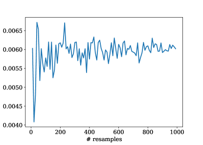
Figure 2: The value of $\sigma$ for different resampling numbers in bootstrapping.

The previous way of estimating error bars is based on theoretical assumptions and, even though it provides useful analytical expressions, it may underestimate unknown sources of errors such as systematic errors.

A brute-force way of estimating error bars is to repeat the estimation of the quantity of interest (in our case $h_{d}$) with $N$ independent experiments and to evaluate the empirical variance of the results. This method can be expensive with respect to classical and quantum computational resources, and the results can be sensitive to how the independent samples are grouped. So while we can split independent samples into five groups of $n_{c}=100$ circuits to estimate the standard deviation this way, a more feasible alternative is instead given by bootstrapping. This is a statistical inference technique in which, instead of performing $N$ new experiments, one resamples the raw results of a single experiment $N$ times in order to estimate properties of the underlying statistical distribution.

In our specific quantum volume experiment, the heavy-output probability $h_{d}$ is estimated as an average over $n_{C}$ random circuits $C$ as shown in equation (10). Let us define the set $S=\{E_{C_{1}},E_{C_{2}},....E_{C_{n_{C}}}\}$ containing all the estimated heavy-output probabilities associated with different random circuits. We can now resample N sets of data $S_{1},S_{2},....S_{N}$, each one containing $n_{c}$ values that are randomly sampled from $S$ with replacements. For each resampled set $S_{j}$ we evaluate the associated bootstrapped mean $\mu_{j}=\langle E_{C}\rangle_{S_{j}}$.

The empirical standard deviation of all the bootstrap means $\{\mu_{1},\mu_{2},...\mu_{N}\}$ provides an estimate of the statistical uncertainty:

$$\sigma=\sqrt{\frac{1}{N}\sum_{j=1}^{N}(\mu_{j}-\bar{\mu})^{2}}.$$ (12)

where $\bar{\mu}=\sum_{j=1}^{N}\mu_{j}/N$. This is the method that we used to evaluate error bars in Fig. 1 (with $N=500$).

One may ask how large should $N$ be, in order to obtain a resonable estimate of the error. In Fig. 2 we show the dependance of $\sigma$ for an arbitrary error-mitigated point of Fig. 1 (the results are qualitatively similar for all points). Fig. 2 provides empirical evidence that, for $N>400$, the bootstrapped estimate converges around a stable result.

References

- Cross et al. [2018] A. W. Cross, L. S. Bishop, S. Sheldon, P. D. Nation, and J. M. Gambetta, Validating quantum computers using randomized model circuits, (2018), 10.1103/PhysRevA.100.032328.
- Jurcevic et al. [2021] P. Jurcevic, A. Javadi-Abhari, L. S. Bishop, I. Lauer, D. F. Bogorin, M. Brink, L. Capelluto, O. Günlük, T. Itoko, N. Kanazawa, A. Kandala, G. A. Keefe, K. Krsulich, W. Landers, E. P. Lewandowski, D. T. McClure, G. Nannicini, A. Narasgond, H. M. Nayfeh, E. Pritchett, M. B. Rothwell, S. Srinivasan, N. Sundaresan, C. Wang, K. X. Wei, C. J. Wood, J.-B. Yau, E. J. Zhang, O. E. Dial, J. M. Chow, and J. M. Gambetta, Demonstration of quantum volume 64 on a superconducting quantum computing system, Quantum Science and Technology 6, 025020 (2021).
- Li and Benjamin [2016] Y. Li and S. C. Benjamin, Efficient variational quantum simulator incorporating active error minimisation, (2016), 10.1103/PhysRevX.7.021050.
- Temme et al. [2016] K. Temme, S. Bravyi, and J. M. Gambetta, Error mitigation for short-depth quantum circuits, (2016), 10.1103/PhysRevLett.119.180509.
- Giurgica-Tiron et al. [2020] T. Giurgica-Tiron, Y. Hindy, R. LaRose, A. Mari, and W. J. Zeng, Digital zero noise extrapolation for quantum error mitigation, 2020 IEEE International Conference on Quantum Computing and Engineering (QCE) , 306–316 (2020), arXiv: 2005.10921.
- [6] IBM Quantum, https://quantum-computing.ibm.com/.
- Kim et al. [2021] Y. Kim, C. J. Wood, T. J. Yoder, S. T. Merkel, J. M. Gambetta, K. Temme, and A. Kandala, Scalable error mitigation for noisy quantum circuits produces competitive expectation values, arXiv:2108.09197 [cond-mat, physics:quant-ph] (2021), arXiv: 2108.09197.
- Huggins et al. [2021] W. J. Huggins, S. McArdle, T. E. O’Brien, J. Lee, N. C. Rubin, S. Boixo, K. B. Whaley, R. Babbush, and J. R. McClean, Virtual distillation for quantum error mitigation, Physical Review X 11, 041036 (2021), arXiv: 2011.07064.
- Koczor [2021] B. Koczor, Exponential error suppression for near-term quantum devices, Physical Review X 11, 031057 (2021), arXiv: 2011.05942.
- Cotler et al. [2019] J. Cotler, S. Choi, A. Lukin, H. Gharibyan, T. Grover, M. E. Tai, M. Rispoli, R. Schittko, P. M. Preiss, A. M. Kaufman, M. Greiner, H. Pichler, and P. Hayden, Quantum virtual cooling, Physical Review X 9, 031013 (2019), arXiv: 1812.02175.
- LaRose et al. [2021] R. LaRose, A. Mari, S. Kaiser, P. J. Karalekas, A. A. Alves, P. Czarnik, M. E. Mandouh, M. H. Gordon, Y. Hindy, A. Robertson, P. Thakre, N. Shammah, and W. J. Zeng, Mitiq: A software package for error mitigation on noisy quantum computers, arXiv:2009.04417 [quant-ph] (2021), arXiv: 2009.04417.
- Kandala et al. [2019] A. Kandala, K. Temme, A. D. Córcoles, A. Mezzacapo, J. M. Chow, and J. M. Gambetta, Error mitigation extends the computational reach of a noisy quantum processor, 567, 491–495 (2019).
- Zhang et al. [2020] S. Zhang, Y. Lu, K. Zhang, W. Chen, Y. Li, J.-N. Zhang, and K. Kim, Error-mitigated quantum gates exceeding physical fidelities in a trapped-ion system, Nature Communications 11, 587 (2020).
- Berg et al. [2022] E. v. d. Berg, Z. K. Minev, A. Kandala, and K. Temme, Probabilistic error cancellation with sparse Pauli-Lindblad models on noisy quantum processors, arXiv:2201.09866 [quant-ph] (2022), arXiv: 2201.09866.
- Bultrini et al. [2021] D. Bultrini, M. H. Gordon, P. Czarnik, A. Arrasmith, P. J. Coles, and L. Cincio, Unifying and benchmarking state-of-the-art quantum error mitigation techniques, arXiv:2107.13470 [quant-ph] (2021), arXiv: 2107.13470.
- Huffman et al. [2021] E. Huffman, M. G. Vera, and D. Banerjee, Real-time dynamics of plaquette models using NISQ hardware, arXiv:2109.15065 [cond-mat, physics:hep-lat, physics:quant-ph] (2021), arXiv: 2109.15065.
- Karalekas et al. [2020] P. J. Karalekas, N. A. Tezak, E. C. Peterson, C. A. Ryan, M. P. da Silva, and R. S. Smith, A quantum-classical cloud platform optimized for variational hybrid algorithms, Quantum Science and Technology 5, 024003 (2020), arXiv: 2001.04449.
- Pino et al. [2021] J. M. Pino, J. M. Dreiling, C. Figgatt, J. P. Gaebler, S. A. Moses, M. S. Allman, C. H. Baldwin, M. Foss-Feig, D. Hayes, K. Mayer, C. Ryan-Anderson, and B. Neyenhuis, Demonstration of the trapped-ion quantum-CCD computer architecture, Nature 592, 209–213 (2021), arXiv: 2003.01293.
- Baldwin et al. [2021] C. H. Baldwin, K. Mayer, N. C. Brown, C. Ryan-Anderson, and D. Hayes, Re-examining the quantum volume test: Ideal distributions, compiler optimizations, confidence intervals, and scalable resource estimations, arXiv:2110.14808 [quant-ph] (2021), arXiv: 2110.14808.