Fully Adaptive Composition in Differential Privacy

Abstract

Composition is a key feature of differential privacy. Well-known advanced composition theorems allow one to query a private database quadratically more times than basic privacy composition would permit. However, these results require that the privacy parameters of all algorithms be fixed before interacting with the data. To address this, Rogers et al. (2016) introduced fully adaptive composition, wherein both algorithms and their privacy parameters can be selected adaptively. They defined two probabilistic objects to measure privacy in adaptive composition: privacy filters, which provide differential privacy guarantees for composed interactions, and privacy odometers, time-uniform bounds on privacy loss. There are substantial gaps between advanced composition and existing filters and odometers. First, existing filters place stronger assumptions on the algorithms being composed. Second, these odometers and filters suffer from large constants, making them impractical. We construct filters that match the rates of advanced composition, including constants, despite allowing for adaptively chosen privacy parameters. En route we also derive a privacy filter for approximate zCDP. We also construct several general families of odometers. These odometers match the tightness of advanced composition at an arbitrary, preselected point in time, or at all points in time simultaneously, up to a doubly-logarithmic factor. We obtain our results by leveraging advances in martingale concentration. In sum, we show that fully adaptive privacy is obtainable at almost no loss.

1 Introduction

Differential privacy (Dwork et al., 2006b) is an algorithmic criterion that provides meaningful guarantees of individual privacy for analyzing sensitive data. Intuitively, an algorithm is differentially private if similar inputs induce similar distributions on outputs. More formally, an algorithm $A:\mathcal{X}\rightarrow\mathcal{Y}$ is differentially private if, for any set of outcomes $G\subset\mathcal{Y}$ and any neighboring inputs $x,x^{\prime}\in\mathcal{X}$,

$$\mathbb{P}(A(x)\in G)\leq e^{\epsilon}\mathbb{P}(A(x^{\prime})\in G)+\delta,$$ (1)

where $\epsilon$ and $\delta$ are the privacy parameters of the algorithm.

A key property of differential privacy is graceful composition. Suppose $A_{1},\dots,A_{n}$ are algorithms such that each $A_{m}$ is $(\epsilon_{m},\delta_{m})$-differentially private. Advanced composition (Dwork et al., 2010; Kairouz et al., 2015) states that, for any $\delta^{\prime}>0$, the composed sequence of algorithms is $(\epsilon,\delta)$-differentially private, where $\delta=\delta^{\prime}+\sum_{m\leq n}\delta_{m}$, and

$$\epsilon=\sqrt{2\log\left(\frac{1}{\delta^{\prime}}\right)\sum_{m\leq n}\epsilon_{m}^{2}}+\sum_{m\leq n}\epsilon_{m}\left(\frac{e^{\epsilon_{m}}-1}{e^{\epsilon_{m}}+1}\right).$$ (2)

When all privacy parameters are the same and small, we roughly have $\epsilon=O(\sqrt{n}\epsilon_{m})$. Hence, analysts can make use of sensitive datasets with a slow degradation of privacy.

However, there is a major disconnect between most existing results on privacy composition and modern data analysis. As analysts view the outputs of algorithms, the future manner in which they interact with the data changes. Advanced composition allows analysts to adaptively select algorithms, but not privacy parameters. In many cases, analysts may wish to choose the subsequent privacy parameters based on the outcomes of the previous private algorithms. For example, if an analyst learns, from past computations, that they only need to run one more computation, they should be able to use the remainder of their privacy budget in the final round. Likewise, if an analyst is having a hard time deriving conclusions, they should be allowed to adjust privacy parameters to extend the allowable number of computations.

This desideratum has motivated the study of fully adaptive composition, wherein one is allowed to adaptively select the privacy parameters of the algorithms. Rogers et al. (2016) define two probabilistic objects which can be used to ensure privacy guarantees in fully adaptive composition. The first, called a privacy filter, is an adaptive stopping condition that ensures an entire interaction between an analyst and a dataset retains a pre-specified target privacy level, even when the privacy parameters are chosen adaptively. The second, called a privacy odometer, provides a sequence of high-probability upper bounds on how much privacy has been lost up to any point in time. While this work took the first steps towards fully adaptive composition, their filters and odometers suffered from large constants and the latter suffered from sub-optimal asymptotic rates.

We show that, as long as a target privacy level is pre-specified, one can obtain the same rate as advanced composition, including constants. We also construct families of privacy odometers that are not only tighter than the originals, but can be optimized for various target levels of privacy. Overall, we show that full adaptivity is not a cost—but rather a feature—of differential privacy.

1.1 Related Work

Privacy Composition:

There is a long line of work on privacy composition. The “basic composition” theorem states that, when composing private algorithms, the privacy parameters (both $\epsilon$ and $\delta$) add up linearly (Dwork et al., 2006b, a; Dwork and Lei, 2009). The “advanced composition” theorem allows the total $\epsilon$ to grow sublinearly with a small degradation on $\delta$ (Dwork et al., 2010). Later work (Kairouz et al., 2015; Murtagh and Vadhan, 2016) studies “optimal” composition, a computationally intractable formula that tightly characterizes the overall privacy of composed mechanisms.

More recently, several variants of privacy have been studied including (zero)-concentrated differential privacy (zCDP) (Bun and Steinke, 2016; Dwork and Rothblum, 2016), Renyi differential privacy (RDP) (Mironov, 2017), and $f$-differential privacy ($f$-DP) (Dong et al., 2021). These all exhibit tighter composition results than differential privacy, but for restricted classes of mechanisms. These results do not allow adaptive choices of privacy parameters.

Privacy Filters and Odometers:

Rogers et al. (2016) originally introduced privacy filters and odometers, which allow privacy composition with adaptively selected privacy parameters. While their contributions provide a decent approximation of advanced composition, their bounds suffer from large constants, which prevents practical usage. Our work directly improves over these initial results. First, we construct privacy filters essentially matching advanced composition. We also provide flexible families of privacy odometers that outperform those of Rogers et al. (2016).

Feldman and Zrnic (2021) leverage RDP to construct Rényi filters, where they require individual mechanisms to satisfy RDP. Since our proof establishes a new privacy filter for approximate zCDP (Bun and Steinke, 2016), our results also extend to approximate RDP (Papernot and Steinke, 2022), which directly generalizes their Rényi filter. Even though it is also possible to obtain a privacy filter for $(\epsilon,\delta)$-DP through Rényi filters (Feldman and Zrnic, 2021), this result requires a stronger assumption that algorithms being composed satisfy probabilistic (i.e.​ point-wise) differential privacy (Kasiviswanathan and Smith, 2014). Since converting from differential privacy to probabilistic differential privacy can be costly (see Lemma 2), our filters demonstrate an improvement by avoiding the conversion cost.

More recently, Koskela et al. (2022) and Smith and Thakurta (2022) provide privacy filters for Gaussian DP (GDP) (Dong et al., 2021). However, their results do not hold for more general mechanisms under $f$-DP and therefore cannot handle algorithms with rare “catastrophic” privacy failure events, in which the privacy loss goes to infinity. Both of our $(\epsilon,\delta)$-filter and approximate zCDP filters can handle such events.

Feldman and Zrnic (2021) and Lécuyer (2021) construct RDP odometers. The former work sequentially composes Rényi filters and the latter work simultaneously runs multiple Rényi filters and takes a union bound. Neither odometer provides high probability, time-uniform bounds on privacy loss, making these results incomparable to our own. We believe our notion of odometers, which aligns with that of Rogers et al. (2016), is more natural.

To prove our results, we leverage time-uniform concentration results for martingales (Howard et al., 2020, 2021). The bounds in these papers directly improve over related self-normalized concentration results (de la Pena et al., 2004; Chen et al., 2014). These latter bounds were leveraged in Rogers et al. (2016) to construct filters and odometers.

(a)

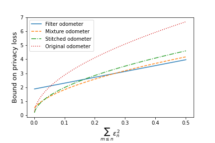
(b)

Figure 1: Figure 1(a) compares the lower order terms of advanced composition and our privacy filter. Figure 1(b) compares the original odometer of Rogers et al. (2016) with our odometers (filter, mixture, and stitched).

1.2 Summary of Contributions

In this work, we provide two primary contributions. We present these results in full rigor following a brief discussion of privacy basics and martingale theory in Section 2.

Privacy Filters:

In Theorem 2 of Section 3, we construct privacy filters that match the rate of advanced composition, significantly improving over results of Rogers et al. (2016). Our filter follows from a more general approximate zCDP/RDP filter (Bun and Steinke, 2016; Papernot and Steinke, 2022) presented in Theorem 1. In particular, this approximate zCDP/RDP filter greatly generalizes existing filters from the pure RDP setting (Feldman and Zrnic, 2021). This extension allows us to capture a broader class of algorithms and avoids the conversion loss when translating bounds between pure RDP and $(\epsilon,\delta)$-differential privacy. We state an informal version of filter in the case of approximate differential privacy below.

Informal Theorem 1 (Improved Privacy Filter).

Fix target privacy parameters $\epsilon>0$ and $\delta>0$, and suppose $(A_{n})_{n\geq 1}$ is an adaptively selected sequence of algorithms. Assume that $A_{n}$ is $(\epsilon_{n},\delta_{n})$-DP conditioned on the outputs of the first $n-1$ algorithms, where $\epsilon_{n}$ and $\delta_{n}$ may depend on outputs of $A_{1},\dots,A_{n-1}$. If a data analyst stops interacting with the data before $\sqrt{2\log\left(\frac{1}{\delta}\right)\sum_{m\leq n+1}\epsilon_{m}^{2}}+\frac{1}{2}\sum_{m\leq n+1}\epsilon_{m}^{2}>\epsilon$, then the entire interaction is $(\epsilon,\delta)$-DP.

Privacy Odometers:

In Theorem 3 of Section 4, we construct improved privacy odometers — that is, sequences of upper bounds on privacy loss which are all simultaneously valid with high probability. Our three families of odometers theoretically and empirically outperform those of Rogers et al. (2016). See Figure 1(b) for a comparison.

For both results, our key insight is to view adaptive privacy composition as depending not on the number of algorithms being composed, but rather on the sums of squares of privacy parameters, $\sum_{m\leq n}\epsilon_{m}^{2}$. This shift to looking at “intrinsic time” allows us to apply recent advances in time-uniform concentration (Howard et al., 2020, 2021) to privacy loss martingales. Overall, our results show that there is essentially no cost for fully adaptive private data analysis.

2 Background on Differential Privacy

Throughout, we assume all algorithms map from a space of datasets $\mathcal{X}$ to outputs in a measurable space, typically either denoted $(\mathcal{Y},\mathcal{G})$ or $(\mathcal{Z},\mathcal{H})$. For a sequence of algorithms $(A_{n})_{n\geq 1}$, we often consider the composed algorithm $A_{1:n}:=(A_{1},\dots,A_{n})$. For more background on measure-theoretic matters, as well as on the notion of neighboring datasets, see Appendix A.

We start by formalizing a generalization of differential privacy in which the privacy parameters of an algorithm $A_{n}$ can be functions of the outputs of $A_{1},\dots,A_{n-1}$. In particular, we replace the probabilities in Equation (1) with conditional probabilities given relevant random variables.

Definition 1 (Conditional Differential Privacy).

Suppose $A$ and $B$ are algorithms mapping from a space $\mathcal{X}$ to measurable spaces $(\mathcal{Y},\mathcal{G})$ and $(\mathcal{Z},\mathcal{H})$ respectively. Suppose $\epsilon,\delta:\mathcal{Z}\rightarrow\mathbb{R}_{\geq 0}$ are measurable functions. We say the algorithm $A$ is $(\epsilon,\delta)$-differentially private conditioned on $B$ if, for any neighbors $x,x^{\prime}\in\mathcal{X}$ and for all measurable sets $G\in\mathcal{G}$, we have

$$\mathbb{P}\left(A(x)\in G\mid B(x)\right)$$

$$\;\;\leq e^{\epsilon(B(x))}\mathbb{P}\left(A(x^{\prime})\in G\mid B(x)\right)+\delta(B(x)).$$

For conciseness, we will write either $\epsilon$ or $\epsilon(x)$ for $\epsilon(B(x))$ and likewise $\delta$ or $\delta(x)$ for $\delta(B(x))$.

In the $n$th round of adaptive composition, we will set $A:=A_{n}$ and $B:=A_{1:n-1}$. In this setting, the analyst has functions $\epsilon_{n},\delta_{n}:\mathcal{Y}^{n-1}\rightarrow\mathbb{R}_{\geq 0}$ and takes the $n$th round privacy parameters to be $\epsilon_{n}(A_{1:n-1}(x))$ and $\delta_{n}(A_{1:n-1}(x))$. In other words, the analyst uses the outcome of the first $n-1$ algorithms to decide the level of privacy for the $n$th algorithm, ensuring that $A_{n}$ is $(\epsilon_{n},\delta_{n})$-differentially private conditioned on $A_{1:n-1}$.

We will also leverage the notion of zero-concentrated differential privacy (zCDP) (Bun and Steinke, 2016), which often provides a cleaner analysis for privacy composition. First, we will recall the definition of Rényi divergence.

Definition 2.

The Rényi divergence from $P$ to $Q$ of order $\lambda\geq 1$ is defined as

$$D_{\lambda}(P\|Q):=\frac{1}{\lambda-1}\log\left(\mathbb{E}_{Y\sim P}\left[\left(\frac{P(Y)}{Q(Y)}\right)^{\lambda-1}\right]\right).$$

The notion of zCDP bounds the Rényi divergence from $A(x)$ to $A(x^{\prime})$ for any neighbors $x$ and $x^{\prime}$. We will focus on a conditional version of a more general definition called approximate zCDP (Bun and Steinke, 2016; Papernot and Steinke, 2022) that permits a small probability of unbounded Rényi divergence. The conditional approximate zCDP definition we provides uses the convex mixture formulation adapted from Papernot and Steinke (2022), since it is more convenient for our proof. In Appendix C.1, we will show that in the case $\delta$ and $\rho$ are constant, this definition is equivalent to the original definition in Bun and Steinke (2016).

Definition 3 (Conditional Approximate zCDP).

Suppose $A:\mathcal{X}\times\mathcal{Z}\to\mathcal{Y}$ with outputs in a measurable space $(\mathcal{Y},\mathcal{G})$. Suppose $\delta,\rho:\mathcal{Y}\rightarrow\mathbb{R}_{\geq 0}$. We say the algorithm $A$ satisfies conditional $\delta(z)$-approximate $\rho(z)$-zCDP if, for all $z\in\mathcal{Z}$ and any neighboring datasets $x,x^{\prime}$, there exist probability transition kernels $P^{\prime},P^{\prime\prime},Q^{\prime},Q^{\prime\prime}:\mathcal{Z}\times\mathcal{G}\rightarrow[0,1]$ such that the conditional outputs are distributed according to the following mixture distributions:

$$A(x;z)\sim(1-\delta(z))P^{\prime}(\cdot\mid z)+\delta(z)P^{\prime\prime}(\cdot\mid z)$$

$$A(x^{\prime};z)\sim(1-\delta(z))Q^{\prime}(\cdot\mid z)+\delta(z)Q^{\prime\prime}(\cdot\mid z),$$

where for all $\lambda\geq 1$, $D_{\lambda}(P^{\prime}(\cdot\mid z)\|Q^{\prime}(\cdot\mid z))\leq\rho(z)\lambda$ and $D_{\lambda}(Q^{\prime}(\cdot\mid z)\|P^{\prime}(\cdot\mid z))\leq\rho(z)\lambda$ for all $z\in\mathcal{Z}$.

We will also use the notions of filtration and martingales.

Filtration and Martingales:

A process $(X_{n})_{n\in\mathbb{N}}$ is said to be a martingale with respect to a filtration $(\mathcal{F}_{n})_{n\in\mathbb{N}}$ if, for all $n\in\mathbb{N}$, (a) $X_{n}$ is $\mathcal{F}_{n}$-measurable, (b) $\mathbb{E}|X_{n}|<\infty$, and (c) $\mathbb{E}(X_{n}\mid\mathcal{F}_{n-1})=X_{n-1}$. Correspondingly, $(X_{n})_{n\in\mathbb{N}}$ is a supermartingale if $\mathbb{E}(X_{n}\mid\mathcal{F}_{n-1})\leq X_{n-1}$. In our context, we will consider the natural filtration $(\mathcal{F}_{n}(x))_{n\in\mathbb{N}}$ generated by $(A_{n}(x))_{n\geq 1}$. In our proofs, we construct the appropriate (super)martingales so that we can leverage the optional stopping theorem and time-uniform concentration to obtain privacy filters and odometers (Ville, 1939; Howard et al., 2020, 2021). We present a full exposition of the mathematical tools in Appendix A and B.

3 Privacy Filters

We now provide our main results on privacy filter. In general, a privacy filter is a function $N$ that takes the privacy parameters of a sequence of private algorithms as input and decides to stop at some point so that the composition of these algorithms satisfies a pre-specified level of privacy. We will first present a privacy filter for approximate zCDP (Theorem 1), which will immediately imply the privacy filter result for $(\epsilon,\delta)$-DP (Theorem 2). Since approximate zCDP bounds Rényi divergence of all orders $\lambda$, our proof for Theorem 1 also directly implies a privacy fiter for approximate RDP (Papernot and Steinke, 2022), which generalizes the RDP filter by Feldman and Zrnic (2021).

Our $(\epsilon,\delta)$-DP filter improves on the rate of the original filter presented in Rogers et al. (2016) and matches the rate of advanced composition that requires pre-fixed choices of privacy parameters. Even though it is also possible to obtain an $(\epsilon,\delta)$-DP filter through the result of Feldman and Zrnic (2021), our privacy filters avoid their conversion costs and provide a tighter bound.

We can now state our general privacy filter in terms of approximate zCDP.

Theorem 1 (Approximate zCDP filter).

Let $(A_{n})_{n\geq 1}$ be an adaptive sequence of algorithms, where $A_{n}:\mathcal{X}\times\mathcal{Y}^{n-1}\rightarrow\mathcal{Y}$. Assume that $\delta_{n},\rho_{n}:\mathcal{Y}^{n-1}\to\mathbb{R}_{\geq 0}$. For any $n\geq 1$, assume that $A_{n}(\cdot;y_{1:n-1})$ is conditionally $\delta_{n}(y_{1:n-1})$-approximate $\rho_{n}(y_{1:n-1})$-zCDP for any prior outcomes $y_{1:n-1}$. We define the function $N:\mathcal{Y}^{\infty}\to\mathbb{N}$ where

$$N(y_{1},y_{2},\cdots)=\inf\left\{n:\sum_{m=1}^{n+1}\rho_{\ell}(y_{1:m-1})>\rho\right\}\land\inf\left\{n:\sum_{m=1}^{n+1}\delta_{m}(y_{1:m-1})>\delta\right\}.$$

Then $A_{1:N(\cdot)}(\cdot)$ is $\delta$-approximate $\rho$-zCDP, where $N(x)=N((A_{n}(x))_{n\geq 1}).$

We note that the argument used to prove the above theorem immediately implies a privacy filter for approximate RDP, and thus Theorem 1 can be viewed as a strict generalization of the work of Feldman and Zrnic (2021). Further, Theorem 1 implies a privacy filter under $(\epsilon,\delta)$-differential privacy. To show this implication, we will use the following conversion results.

Lemma 1 ((Bun and Steinke, 2016)).

If $A$ satisfies $(\epsilon,\delta)$-DP, then $A$ satisfies $\delta$-approximate $\frac{1}{2}\epsilon^{2}$-zCDP. If $A$ satisfies $\delta$-approximate $\rho$-zCDP, then $A$ satisfies $(\rho+2\sqrt{\rho\ln(1/\delta^{\prime})},\delta+(1-\delta)\delta^{\prime})$-DP.

We can now obtain our $(\epsilon,\delta)$-privacy filter by a conversion of individual approximate differential privacy parameters to approximate zCDP ones, application of the approximate zCDP filter, and the conversion of approximate zCDP back to approximate differential privacy.

Theorem 2 ($(\epsilon,\delta)$-DP filter).

Suppose $(A_{n})_{n\geq 1}$ is a sequence of algorithms such that, for any $n\geq 1$, $A_{n}$ is $(\epsilon_{n},\delta_{n})$-differentially private conditioned on $A_{1:n-1}$. Let $\epsilon>0$ and $\delta=\delta^{\prime}+\delta^{\prime\prime}$ be target privacy parameters such that $\delta^{\prime}>0,\delta^{\prime\prime}\geq 0$ and for all outcomes $y=(y_{1},y_{2},\cdots)$ we have $\sum_{n=1}^{\infty}\delta_{n}(y_{1:n-1})\leq\delta$. We define the function $N:\mathcal{Y}^{\infty}\to\mathbb{N}$ where

$$N(y_{1},y_{2},\cdots)=\inf\left\{n:\sum_{m=1}^{n+1}\epsilon^{2}_{\ell}(y_{1:m-1})/2>\rho\right\}\land\inf\left\{n:\sum_{m=1}^{n+1}\delta_{m}(y_{1:m-1})>\delta\right\}.$$

Then, the algorithm $A_{1:N(\cdot)}(\cdot)$ is $(\rho+2\sqrt{\rho\log(1/\delta)},\delta)$-DP, where $N(x):=N((A_{n}(x))_{n\geq 1}).$

Proof of Theorem 1.

In our proof, we assume that $\sum_{n=1}^{\infty}\delta_{n}(y_{1:n-1})\leq\delta$ for all sequences $(y_{n})_{n\geq 1}$ without loss of generality. Let $P_{1:n}$ and $Q_{1:n}$ denote the joint distributions of $(A_{1},\dots,A_{n})$ with inputs $x$ and $x^{\prime}$, respectively. We overload notation and write $P_{1:n}(y_{1},\dots,y_{n})$ and $Q_{1:n}(y_{1},\dots,y_{n})$ for the likelihood of $y_{1},\dots,y_{n}$ under input $x$ and $x^{\prime}$ respectively. We similarly write $P_{n}(y_{n}\mid y_{1:n-1})$ and $Q_{n}(y_{n}\mid y_{1:n-1})$ for the corresponding conditional densities.

By Bayes rule, for any $n\in\mathbb{N},$ we have

$$P_{1:n}(y_{1},\cdots,y_{n}) =\prod_{m=1}^{n}P_{m}(y_{m}\mid y_{1:m-1}),$$

$$Q_{1:n}(y_{1},\cdots,y_{n}) =\prod_{m=1}^{n}Q_{m}(y_{m}\mid y_{1:m-1}).$$

By our assumption of approximate zCDP at each step $n$, we can write the conditional likelihoods of $P_{n}$ and $Q_{n}$ as the following convex combinations:

$$P_{n}(y_{n}\mid y_{1:n-1}) =(1-\delta_{n}(y_{1:n-1}))P^{\prime}_{n}(y_{n}\mid y_{1:n-1})+\delta_{n}(y_{1:n-1})P^{\prime\prime}_{n}(y_{n}\mid y_{1:n-1}),$$

$$Q_{n}(y_{n}\mid y_{1:n-1}) =(1-\delta_{n}(y_{1:n-1}))Q^{\prime}_{n}(y_{n}\mid y_{1:n-1})+\delta_{n}(y_{1:n-1})Q^{\prime\prime}_{n}(y_{n}\mid y_{1:n-1}),$$

such that for all $\lambda\geq 1$ and all prior outcomes $y_{1:n-1}$, we have both

$$D_{\lambda}\left(P_{n}^{\prime}(\cdot\mid y_{1:n-1})\leavevmode\nobreak\ \|\leavevmode\nobreak\ Q_{n}^{\prime}(\cdot\mid y_{1:n-1})\right)\leq\rho_{n}(y_{1:n-1})\lambda,$$ (3)

$$D_{\lambda}\left(Q_{n}^{\prime}(\cdot\mid y_{1:n-1})\leavevmode\nobreak\ \|\leavevmode\nobreak\ P_{n}^{\prime}(\cdot\mid y_{1:n-1})\right)\leq\rho_{n}(y_{1:n-1})\lambda.$$ (4)

Now, from Lemma 7, we can then write these distributions as a convex combination of “good” distributions for which Rényi divergence is small, and “bad” distributions for which the divergence may be unbounded. In more detail, using the assumption that $\sum_{n=1}^{\infty}\delta_{n}(y_{1:n-1})\leq\delta$ for all seqeunces $(y_{n})_{n\geq 1},$ we have, for all $n\geq 1$,

$$P_{1:n}(y_{1},\cdots,y_{n}) =(1-\delta)\underbrace{\prod_{m=1}^{n}P_{m}^{\prime}(y_{m}|y_{1:m-1})}_{P_{1:n}^{\prime}(y_{1},\cdots,y_{n})}+\delta P_{1:n}^{\prime\prime}(y_{1},\cdots,y_{n})$$ (5)

$$Q_{1:n}(y_{1},\cdots,y_{n}) =(1-\delta)\underbrace{\prod_{m=1}^{n}Q_{m}^{\prime}(y_{m}|y_{1:m-1})}_{Q_{1:n}^{\prime}(y_{1},\cdots,y_{n})}+\delta Q_{1:n}^{\prime\prime}(y_{1},\cdots,y_{n}).$$ (6)

From the above, if $N:\mathcal{Y}^{\infty}\rightarrow\mathbb{N}$ is the time outlined in the theorem statement, it follows that the joint densities $P_{1:N}$ of $A_{1}(x),\cdots A_{N(x)}(x)$ and $Q_{1:N}$ of $A_{1}(x^{\prime}),\cdots A_{N(x^{\prime})}(x^{\prime})$, and both can be written as a convex combination of distributions $(P_{1:N}^{\prime},P_{1:N}^{\prime\prime})$ and $(Q_{1:N}^{\prime},Q_{1:N}^{\prime\prime})$:

$$P_{1:N}(y_{1},y_{2},\cdots,y_{N}) =(1-\delta)\underbrace{\prod_{n=1}^{N}P_{n}^{\prime}(y_{n}|y_{1:n-1})}_{P^{\prime}(y_{1},y_{2},\cdots,y_{N})}+\delta P_{1:N}^{\prime\prime}(y_{1},y_{2},\cdots,y_{N})$$

$$Q_{1:N}(y_{1},y_{2},\cdots,y_{N}) =(1-\delta)\underbrace{\prod_{n=1}^{N}Q_{n}^{\prime}(y_{n}|y_{1:n-1})}_{Q^{\prime}(y_{1},y_{2},\cdots,y_{N})}+\delta Q_{1:N}^{\prime\prime}(y_{1},y_{2},\cdots,y_{N})$$

In the above, we notate quantities in terms of “$N$” instead of “$N(x)$” or “$N(x^{\prime})$” since $N$ only depends on the underlying dataset $x$ or $x^{\prime}$ through the observed sequence of iterates $(y_{n})_{n\geq 1}$.

What remains now is to bound the Rényi divergence between $P_{N}^{\prime}$ and $Q_{N}^{\prime}$. We do this using an optional stopping argument for non-negative supermartingales (Lemma 5). Suppose $(Y_{n}^{\prime})_{n\geq 1}$ is a process whose $n$th finite-dimensional distribution is given by $P_{n}^{\prime}$. For any fixed $\lambda\geq 1$, define the process $(M_{n}^{(\lambda)})_{n\geq 0}$ by:

$$M_{n}^{(\lambda)} :=\exp\left\{(\lambda-1)\sum_{m\leq n}\left[\log\left(\frac{P^{\prime}_{m}(Y_{m}^{\prime}\mid Y_{1:m-1}^{\prime})}{Q^{\prime}_{m}(Y_{m}^{\prime}\mid Y_{1:m-1}^{\prime})}\right)-\lambda\rho_{m}(Y_{1:m-1}^{\prime})\right]\right\}.$$ (7)

It is clear that $M_{n}^{(\lambda)}$ is a non-negative supermartingale with respect to natural filtration $(\mathcal{F}_{n}^{\prime})_{n\geq 1}$ given by $\mathcal{F}_{n}^{\prime}:=\sigma(Y_{m}^{\prime}:m\leq n)$, a fact that we confirm in Lemma 6. We emphasize that $(\mathcal{F}_{n}^{\prime})_{n\geq 1}$ is not in fact the data generating filtration, but rather a tool used for theoretical analysis. In more detail, we consider this filtration because, heuristically, approximate zCDP aims at bounding the moment generating function of a “good” portion of the joint distribution — the true joint distribution may allow some probability of catastrophic failure (i.e. unbounded privacy loss). We adopt the same convention that $N:=N(y_{1},y_{2},\dots)$ with the explicit values of $(y_{n})_{n\geq 1}$ clear from context. Observe that $N((Y_{n}^{\prime})_{n\geq 1})$ is a stopping time with respect to $(\mathcal{F}_{n}^{\prime})_{n\geq 0}$. We now invoke optional stopping (Lemma 5), which yields

$$\mathbb{E}[M_{N(Y_{1}^{\prime},Y_{2}^{\prime},\dots)}^{(\lambda)}]\leq 1 \implies\mathbb{E}\left[\exp\left((\lambda-1)\sum_{n\leq N(Y_{1}^{\prime},Y_{2}^{\prime},\cdots)}\left\{\log\left(\frac{P^{\prime}_{n}(Y_{n}^{\prime}\mid Y_{1:n-1}^{\prime})}{Q^{\prime}_{n}(Y_{n}^{\prime}\mid Y_{1:n-1}^{\prime})}\right)-\lambda\rho_{n}(Y_{1:n-1}^{\prime})\right\}\right)\right]\leq 1$$

$$\implies\mathbb{E}\left[\exp\left((\lambda-1)\sum_{n\leq N(Y_{1}^{\prime},Y_{2}^{\prime},\cdots)}\log\left(\frac{P^{\prime}_{n}(Y_{n}^{\prime}\mid Y_{1:n-1}^{\prime})}{Q^{\prime}_{n}(Y_{n}^{\prime}\mid Y_{1:n-1}^{\prime})}\right)\right)\right]\leq e^{\lambda(\lambda-1)\rho}$$

$$\implies\mathbb{E}\left[\exp\left((\lambda-1)\log\left(\frac{P^{\prime}_{N}(Y_{1:N}^{\prime})}{Q^{\prime}_{N}(Y_{1:N}^{\prime})}\right)\right)\right]\leq e^{\lambda(\lambda-1)\rho}.$$

What we have just showed is precisely that

$$D_{\lambda}\left(P_{N}^{\prime}\mid Q_{N}^{\prime}\right)\leq\rho\lambda,$$

which is precisely the desired result. A symmetric argument yields an identical bound on $D_{\lambda}(Q_{N}^{\prime}\mid P_{N}^{\prime})$. Thus, we have showed the desired result. ∎

4 Privacy Odometers

Previously, we constructed privacy filters that matched the rate of advanced composition while allowing both algorithms and privacy parameters to be chosen adaptively. While privacy filters require the total level of privacy to be fixed in advance, it is desirable to track the privacy loss at all steps without a pre-fixed budget (Ligett et al., 2017). We now study privacy odometers which provide sequences of upper bounds on accumulated privacy loss that are valid at all points in time simultaneously with high probability.

4.1 Background on Privacy Loss and Odometers

To formally introduce privacy odometers, we will first revisit the notion of privacy loss, which measures how much information is revealed about the underlying input dataset. For neighbors $x,x^{\prime}\in\mathcal{X}$, let $p^{x}$ and $p^{x^{\prime}}$ be the densities of $A(x)$ and $A(x^{\prime})$ respectively. The privacy loss between $A(x)$ and $A(x^{\prime})$ is defined as

$$\mathcal{L}(x,x^{\prime}):=\log\left(\frac{p^{x}(A(x))}{p^{x^{\prime}}(A(x))}\right).$$ (8)

By Equation (8), a negative privacy loss suggests that the input is more likely to be $x^{\prime}$, and likewise a positive privacy loss suggests that the input is more likely to be $x$. We now generalize privacy loss to its conditional counterpart.

Definition 4 (Conditional Privacy Loss).

Suppose $A$ and $B$ are as in Definition 1. Suppose $x,x^{\prime}\in\mathcal{X}$ are neighbors. Let $p^{x}(\cdot|\cdot),p^{x^{\prime}}(\cdot|\cdot):\mathcal{Y}\times\mathcal{Z}\rightarrow\mathbb{R}_{\geq 0}$ be conditional densities for $A(x)$ and $A(x^{\prime})$ respectively given $B(x)$. The privacy loss between $A(x)$ and $A(x^{\prime})$ conditioned on $B$ is given by

$$\mathcal{L}_{B}(x,x^{\prime}):=\log\left(\frac{p^{x}(A(x)|B(x))}{p^{x^{\prime}}(A(x)|B(x))}\right).$$

Suppose $A_{n}$ is the $n$th algorithm being run and we have already observed $A_{1:n-1}(x)$ for some unknown input $x\in\mathcal{X}$. If we are trying to guess whether $x$ or a neighbor $x^{\prime}$ produced the data, we would consider the privacy loss between $A_{n}(x)$ and $A_{n}(x^{\prime})$ conditioned on $A_{1:n-1}(x)$. It is straightforward to characterize the privacy loss of a composed algorithm $A_{1:n}$ in terms of the privacy loss of each constituent algorithm $A_{1},\cdots,A_{n}$. Namely, from Bayes rule,

$$\mathcal{L}_{1:n}(x,x^{\prime})=\sum_{m\leq n}\mathcal{L}_{m}(x,x^{\prime}),$$ (9)

where $\mathcal{L}_{m}(x,x^{\prime})$ is shorthand for the conditional privacy loss between $A_{m}(x)$ and $A_{m}(x^{\prime})$ given $A_{1:m-1}(x)$, per Definition 4. Equation (9) also holds at arbitrary random times $N(x)$ that only depend on the dataset $x\in\mathcal{X}$ through observed algorithm outputs.

The simple decomposition of privacy loss noted above motivates the study of an “alternative”, probabilistic definition of differential privacy. Intuitively, an algorithm should be differentially private if, with high probability, the privacy loss is small. More formally, an algorithm $A:\mathcal{X}\rightarrow\mathcal{Y}$ is said to be $(\epsilon,\delta)$-probabilistically differentially private, or $(\epsilon,\delta)$-pDP for short, if, for all neighboring inputs $x,x^{\prime}\in\mathcal{X}$, we have $\mathbb{P}\left(|\mathcal{L}(x,x^{\prime})|>\epsilon\right)\leq\delta$. In the previous line (as well as in the remainder of the section), the randomness in $\mathcal{L}(x,x^{\prime})$ comes from the randomized algorithm $A$.

Unfortunately, as noted by Kasiviswanathan and Smith (2014) (in which pDP is called point-wise indistinguishability), pDP is a strictly stronger notion than DP. In particular, if an algorithm is $(\epsilon,\delta)$-pDP, it is also $(\epsilon,\delta)$-DP. The converse in general requires a costly conversion.

Lemma 2 (Conversions between DP and pDP (Kasiviswanathan and Smith, 2014)).

If $A$ is $(\epsilon,\delta)$-pDP, then $A$ is also $(\epsilon,\delta)$-DP. Conversely, if $A$ is $(\epsilon,\delta)$-DP, then $A$ is $(2\epsilon,\frac{2\delta}{\epsilon e^{\epsilon}})$-pDP.

We note that that Guingona et al. (2023) have recently shown that other possible conversion rates from probabilistic differential privacy to approximate differential privacy are possible. However, we note that these conversions require trading off tightness in the approximation parameter $\epsilon$ and the approximation parameter $\delta$. In particular, a fully tight conversion from probabilistic differenial privacy to approximate differential privacy is not possible. We will work with the conditional counterpart of probabilistic differential privacy (pDP).

Definition 5 (Conditional Probabilistic Differential Privacy).

Suppose $A:\mathcal{X}\rightarrow\mathcal{Y}$ and $B:\mathcal{X}\rightarrow\mathcal{Z}$ are algorithms, and $\epsilon,\delta:\mathcal{Z}\rightarrow\mathbb{R}_{\geq 0}$ are measurable. Then, $A$ is said to be $(\epsilon,\delta)$-probabilistically differentially private conditioned on $B$ if, for any neighbors $x,x^{\prime}\in\mathcal{X}$, we have

$$\mathbb{P}\left(|\mathcal{L}_{B}(x,x^{\prime})|>\epsilon(B(x))|B(x)\right)\leq\delta(B(x)).$$

While in Theorem 2 we assumed that the algorithms being composed were conditionally differentially private, here, we need to assume conditional probabilistic privacy. This is because our goal is not differential privacy, but rather tight control over privacy loss. We conjecture that a version of our privacy odometer (in Theorem 3) that replaces pDP by DP and leaves all else identical does not hold. Our intuition for this conjecture is that there exist simple examples of algorithms satisfying $(\epsilon,\delta)$-DP that don’t satisfy $(\epsilon,\delta)$-pDP (see Appendix F, for instance). We believe that, by sequentially composing such algorithms and using anti-concentration results, one can show that some odometers fail to be valid. We leave this as potential future work. In sequential composition, we would assume the $n$th algorithm $A_{n}$ is $(\epsilon_{n},\delta_{n})$-pDP conditioned on $A_{1:n-1}$. The privacy parameters would be given as functions of $A_{1:n-1}(x)$. Now we state the definition of privacy odometer, which provides bounds on privacy loss under arbitrary stopping conditions (e.g.​ conditions based on model accuracy).

Definition 6 (Privacy Odometer (Rogers et al., 2016)).

Let $(A_{n})_{n\geq 1}$ be an adaptive sequence of algorithms such that, for all $n\geq 1$, $A_{n}$ is $(\epsilon_{n},\delta_{n})$-pDP conditioned on $A_{1:n-1}$. Let $(u_{n})_{n\geq 1}$ be a sequence of functions where $u_{n}:\mathbb{R}^{n-1}_{\geq 0}\times\mathbb{R}^{n-1}_{\geq 0}\rightarrow\mathbb{R}_{\geq 0}$. Let $\delta\in(0,1)$ be a target confidence parameter. For $x\in\mathcal{X},n\geq 1$, define $U_{n}(x):=u_{n}(\epsilon_{1:n-1}(x),\delta_{1:n-1}(x))$. Then, $(u_{n})_{n\geq 1}$ is called a $\delta$-privacy odometer if, for all $x,x^{\prime}\in\mathcal{X}$ neighbors, we have

$$\mathbb{P}\left(\exists n\geq 1:\mathcal{L}_{1:n}(x,x^{\prime})>U_{n}(x)\right)\leq\delta.$$

4.2 Improved Privacy Odometers

We construct our privacy odometers in Theorem 3. Our technical centerpiece is time-uniform concentration inequalities for martingales (Ville, 1939; Howard et al., 2020, 2021). For a martingale $(M_{n})_{n\in\mathbb{N}}$ and confidence level $\delta>0$, time-uniform concentration inequalities provides bounds $(U_{n})_{n\in\mathbb{N}}$ satisfying $\mathbb{P}(\exists n\in\mathbb{N}:M_{n}>U_{n})\leq\delta$. Thus, if we can create a martingale from privacy loss, we can use time-uniform concentration to construct odometers. Our proof first considers the case where each $A_{n}$ is $(\epsilon_{n},0)$-pDP and the privacy loss martingale $(M_{n})_{n\in\mathbb{N}}$  (Dwork et al., 2010) is given by $M_{0}=0$ and:

$$M_{n}:=M_{n}(x,x^{\prime}):=\mathcal{L}_{1:n}(x,x^{\prime})-\sum_{m\leq n}\mathbb{E}\left(\mathcal{L}_{m}(x,x^{\prime})|\mathcal{F}_{n-1}(x)\right)$$ (10)

We then extend to the case of $\delta_{n}\geq 0$ via conditioning.

To construct their filters and odometers, Rogers et al. (2016) use self-normalized concentration inequalities (de la Pena et al., 2004; Chen et al., 2014). We instead use advances in time-uniform martingale concentration (Howard et al., 2020, 2021), which yields tighter results.

Theorem 3.

Suppose $(A_{n})_{n\geq 1}$ is a sequence of algorithms such that, for any $n\geq 1$, $A_{n}$ is $(\epsilon_{n},\delta_{n})$-pDP conditioned on $A_{1:n-1}$. Let $\delta=\delta^{\prime}+\delta^{\prime\prime}$ be a target approximation parameter such that $\delta^{\prime}>0,\delta^{\prime\prime}\geq 0$. Define $N:=N((\delta_{n})_{n\geq 1}):=\inf\left\{n\in\mathbb{N}:\delta^{\prime\prime}<\sum_{m\leq n+1}\delta_{m}\right\}$ and $V_{n}:=\sum_{m\leq n}\epsilon_{m}^{2}$. Define the following:

1. Filter odometer. For any $\epsilon>0$, let $y^{\ast}:=\left(-\sqrt{2\log\left(\frac{1}{\delta^{\prime}}\right)}+\sqrt{2\log\left(\frac{1}{\delta^{\prime}}\right)+\epsilon}\right)^{2}$. Define functions $(u_{n}^{F})_{n\geq 1}$ by

   $$u_{n}^{F}(\epsilon_{1:n},\delta_{1:n}):=\begin{cases}\infty&n>N\\ \frac{\sqrt{2y^{\ast}\log\left(\frac{1}{\delta^{\prime}}\right)}}{2}+\frac{\sqrt{2\log\left(\frac{1}{\delta^{\prime}}\right)}}{2\sqrt{y^{\ast}}}V_{n}+\frac{1}{2}V_{n}&\text{otherwise}.\end{cases}$$

2. Mixture odometer. For any $\gamma>0$, define the sequence of functions $(u_{n}^{M})_{n\geq 1}$ by

   $$u_{n}^{M}(\epsilon_{1:n},\delta_{1:n}):=\begin{cases}\infty&n>N\\ \sqrt{2\log\left(\frac{1}{\delta^{\prime}}\sqrt{\frac{V_{n}+\gamma}{\gamma}}\right)\left(\gamma+V_{n}\right)}+\frac{1}{2}V_{n}&\text{otherwise}.\end{cases}$$

3. Stitched odometer. For any $v_{0}>0$, define the sequence of functions $(u_{n}^{S})_{n\geq 1}$ by

   $$u_{n}^{S}(\epsilon_{1:n},\delta_{1:n}):=\begin{cases}\infty&n>N\text{ or }V_{n}<v_{0}\\ 1.7\sqrt{V_{n}\left(\log\log\left(\frac{2V_{n}}{v_{0}}\right)+0.72\log\left(\frac{5.2}{\delta^{\prime}}\right)\right)}+\frac{1}{2}V_{n}&\text{else}.\end{cases}$$

Then, any of the sequences $(u_{n}^{F})_{n\geq 1}$, $(u_{n}^{M})_{n\geq 1}$, or $(u_{n}^{S})_{n\geq 1}$ is a $\delta$-privacy odometer.

The proof of Theorem 3 can be found in Appendix E. We now provide intuition for our odometers, which are plotted in Figure 3. Our insight is to view odometers not as functions of the number of algorithms being composed, but rather as functions of the intrinsic time $\sum_{m\leq n}\epsilon_{m}^{2}$. This reframing allows us to leverage the various time-uniform concentration inequalities discussed in Appendix B. The filter odometer is the tightest odometer when the value $\sum_{m\leq n}\epsilon_{m}^{2}$ is close to a fixed accumulated variance $y^{\ast}$, but the tightness drops off precipitously when $\sum_{m\leq n}\epsilon_{m}^{2}$ is far from $y^{\ast}$. The mixture odometer, which is named after the the method of mixtures (Robbins, 1970; de la Peña et al., 2007; Howard et al., 2021), sacrifices tightness at any fixed point in time to obtain overall tighter bounds on privacy loss. This odometer can be numerically optimized, in terms of $\rho$, for tightness at a predetermined value $\sum_{m\leq n}\epsilon_{m}^{2}$. The stitched odometer, whose name derives from Theorem 6, is similarly tight across time. This odometer requires that $\sum_{m\leq n}\epsilon_{m}^{2}$ exceed some pre-selected “variance” $v_{0}$ before becoming nontrivial (i.e. finite). Larger values of $v_{0}$ will yield tighter odometers, albeit at the cost of losing bound validity when accumulated variance is small. With this intuition, we can compare our odometers to the original presented in Rogers et al. (2016).

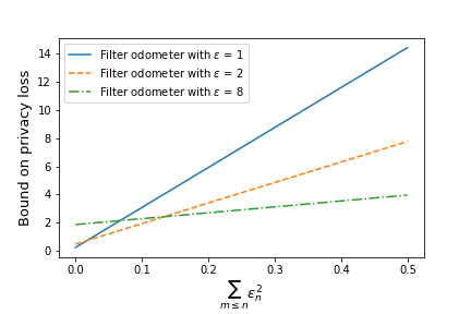
(a)

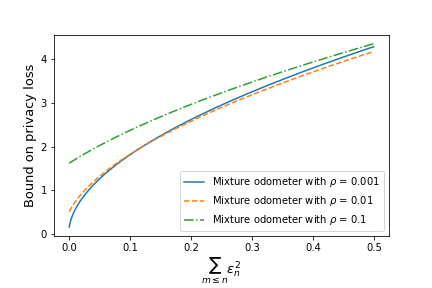
(b)

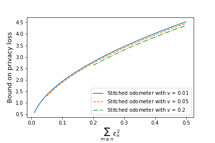
(c)

Figure 2: Comparison of filter, mixture, and stitched odometers plotted as functions of $\sum_{m\leq n}\epsilon_{m}^{2}$. We set $\delta^{\prime}=10^{-6}$ and assume all algorithms being composed are purely differentially private for simplicity.

(a)

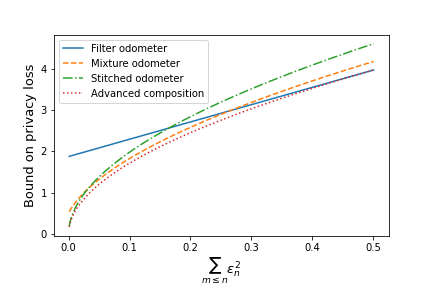
(b)

Figure 3: Figure 3(a) compares our odometers to the original. Figure 3(b) compares them with advanced composition optimized point-wise. The curve plotted for advanced composition is valid at any fixed time, but not uniformly over time. Our odometers nevertheless provide a close approximation.

Lemma 3 (Theorem 6.5 in Rogers et al. (2016)).

Assume the same setup as Theorem 3, and fix $\delta=\delta^{\prime}+\delta^{\prime\prime}$, where $\frac{1}{e}\geq\delta^{\prime}>0$ and $\delta^{\prime\prime}\geq 0$. Define the sequence of functions $(u_{n}^{R})_{n\geq 1}$ by

$$u_{n}^{R}(\epsilon_{1:n},\delta_{1:n}):=\begin{cases}\infty,&n>N\\ \sqrt{2V_{n}\left(\log(110e)+2\log\left(\frac{\log(|x|)}{\delta^{\prime}}\right)\right)}+\frac{1}{2}V_{n}&n\leq N,V_{n}\in\left[\frac{1}{|x|^{2}},1\right]\\ \sqrt{2\left(\frac{1}{|x|^{2}}+V_{n}\right)\left(1+\frac{1}{2}\log\left(1+|x|^{2}V_{n}\right)\right)\log\log\left(\frac{4}{\delta^{\prime}}\log_{2}(|x|)\right)}&+\frac{1}{2}V_{n},\\ &\text{otherwise}\end{cases},$$

where $|x|$ denotes the number of elements in dataset $x$. Then, $(u_{n}^{R})_{n\geq 1}$ is a $\delta$-privacy odometer.

Our new odometers improve over the one presented in Lemma 3. First, the above odometer has an explicit dependence on dataset size. In learning settings, datasets are large, degrading the quality of the odometer. Secondly, the tightness of the odometer drops off outside of the interval $\left[\frac{1}{|x|^{2}},1\right]$. If any privacy parameter of an algorithm being composed exceeds $1$, the bound becomes significantly looser. Lastly, and perhaps most simply, the form of the odometer is complicated. Our odometers all have relatively straightforward dependence on the intrinsic time $\sum_{m\leq n}\epsilon_{m}^{2}$.

We now examine the rates of all odometers. For simplicity, let $v:=\sum_{m\leq n}\epsilon_{m}^{2}$. The stitched odometer has a rate of $O(\sqrt{v\log\log(v)})$ in its leading term, asymptotically matching the law of the iterated logarithm (Robbins, 1970) up to constants. Both the original privacy odometer and the mixture odometer have a rate of $O(\sqrt{v\log\left(v\right)})$, demonstrating worse asymptotic performance. The filter odometer has the worst asymptotic performance, growing linearly as $O\left(v\right)$. This does not mean the stitched odometer is the best odometer, since target levels of privacy are often kept small.

To empirically compare odometers, it suffices to consider the setting of pure differential privacy, as the odometers identically depend on $(\delta_{n})_{n\geq 1}$. Each presented odometer can be viewed as a function of $v$, allowing us to compare odometers by plotting their values for a continuum of $v$. Figure 3(a) shows that there is no clearly tightest odometer. All odometers, barring the original, dominate for some window of values of $v$. While the stitched odometer is asymptotically best, the mixture odometer is tighter for small values of $v$. Likewise, if one knows an approximate target privacy level, the filter odometer is tightest. This behavior is expected from our understanding of martingale concentration (Howard et al., 2020, 2021): there is no uniformly tightest boundary containing (with probability $1-\delta$) the entire path of a martingale; boundaries that are tight early must be looser later, and vice versa. In fact, we conjecture that our bounds are essentially unimprovable in general — this conjecture stems from the fact that the time-uniform martingale boundaries employed have error probability essentially equal to $\delta$, which in turn stems from the deep fact that for continuous-path (and thus continuous-time) martingales, Ville’s inequality (Fact 4)—that underlies the derivation of these boundaries—holds with exact equality. Since we operate in discrete-time, the only looseness in Ville’s inequality stems from lower-order terms that reflect the possibility that at the stopping time, the value of the stopped martingale may not be exactly the value at the boundary.

In Figure 3(b), we compare our odometers with advanced composition optimized in a point-wise sense for all values of $v$ simultaneously. This boundary is not a valid odometer, as advanced composition only holds at a prespecified point in intrinsic time $v$. Our odometers are almost tight with advanced composition for the values of $v$ plotted. Our filter odometer lies tangent to the advanced composition curve, as expected from Section 5.2 of Howard et al. (2020).

5 Future Directions

There are many open problems related to fully adaptive composition. For example, even though privacy filters have been studied under the notion of Gaussian DP (Smith and Thakurta, 2022; Koskela et al., 2022), privacy filters and odometers have not been studied for general $f$-DP (Dong et al., 2021). It also has not been investigated whether adaptivity in privacy parameter selection improves the performance of iterative algorithms such as private SGD. Intuitively, it should be beneficial to let the iterates of an algorithm guide future choices of privacy parameters. Optimal composition results (Kairouz et al., 2015; Murtagh and Vadhan, 2016; Zhu et al., 2022) have yet to be considered in a setting where privacy parameters are adaptively selected. In Appendix D, we provide another proof of Theorem 2, which leverages a reduction of private algorithms to generalized randomized response. Since such a reduction was used in the proofs of Kairouz et al. (2015) and Murtagh and Vadhan (2016), we believe this proof can be useful for optimal composition with adaptively chosen privacy parameters.

Acknowledgements

AR acknowledges support from NSF DMS 1916320 and an ARL IoBT CRA grant. Research reported in this paper was sponsored in part by the DEVCOM Army Research Laboratory under Cooperative Agreement W911NF-17-2-0196 (ARL IoBT CRA). The views and conclusions contained in this document are those of the authors and should not be interpreted as representing the official policies, either expressed or implied, of the Army Research Laboratory or the U.S. Government. The U.S. Government is authorized to reproduce and distribute reprints for Government purposes notwithstanding any copyright notation herein. ZSW and JW were supported in part by the NSF CNS2120667, NSF Award #2120667, a CyLab 2021 grant, a Google Faculty Research Award, and a Mozilla Research Grant. JW acknowledges support from NSF GRFP grants DGE1745016 and DGE2140739.

Appendix A Measure-Theoretic Formalism

Below, we provide some measure-theoretic formalisms and details regarding datasets and neighboring relations.

Neighboring Datasets:

Roughly speaking, an algorithm is differentially private if it difficult to distinguish between output distributions when the algorithm is run on similar inputs. In general, this notion of similarity amongst inputs is defined as a neighboring relation $\sim$ between elements on the input space $\mathcal{X}$. In particular, if two inputs (also referred to as datasets or databases) $x,x^{\prime}\in\mathcal{X}$ satisfy the neighboring relation $x\sim x^{\prime}$, the we say $x$ and $x^{\prime}$ are neighbors.

There are several canonical examples of neighboring relations on the space of inputs $\mathcal{X}$. One example is where $\mathcal{X}=\mathbb{X}^{n}$ for some data domain $\mathbb{X}$. The data domain can be viewed as the set of all possible individual entries for a dataset, and the space $\mathbb{X}^{n}$ correspondingly contains all possible $n$ element datasets. In this setting, databases $x,x^{\prime}\in\mathcal{X}$ may be considered neighbors if $x$ and $x^{\prime}$ differ in exactly one entry. Another slightly more general setting is when $\mathcal{X}=\mathbb{X}^{*}$, i.e., all possible datasets of finite size. In this situation, the earlier notion of neighboring still makes sense. However, in addition, we may say input datasets $x$ and $x^{\prime}$ are neighbors if $x$ can be obtained from $x^{\prime}$ by either adding or deleting an element. This is a very natural notion of neighboring, as under such a relation an algorithm would be differentially private if it were difficult to determine the presence or absence of an individual. Our work is agnostic to the precise choice of neighboring relation. As such, we choose to leave the notion as general as possible.

Algorithms and Random Variables:

We will consider algorithms as randomized mappings $A:\mathcal{X}\rightarrow\mathcal{Y}$ taking inputs from $\mathcal{X}$ to some output space $\mathcal{Y}$. To be fully formal, we consider the output space $\mathcal{Y}$ as a measurable space $(\mathcal{Y},\mathcal{G})$, where $\mathcal{G}$ is some $\sigma$-algebra denoting possible events. Recall that a $\sigma$-algebra $\mathcal{S}$ for a set $S$ is simply a subset of $2^{S}$ containing $S$ and $\emptyset$ that is closed under countable union, intersection, and complements. When we say $A$ is an algorithm having inputs in some space $\mathcal{X}$, we really mean $A(x)$ is a $\mathcal{Y}$-valued random variable for any $x\in\mathcal{X}$. The space $\mathcal{X}$ need not have an associated $\sigma$-algebra, as algorithm inputs are essentially just indexing devices. Given a sequence of algorithms $(A_{n})_{n\geq 1}$, $(A_{n}(x))_{n\geq 1}$ is a sequence of $\mathcal{Y}$-valued random variables, for any $x\in\mathcal{X}$.

Since we are dealing with the composition of algorithms, we write $A_{1:n}(x)$ as shorthand for the random vector of the first $n$ algorithm outputs, i.e. $A_{1:n}(x)=(A_{1}(x),\dots,A_{n}(x))$. Formally, the random vector $A_{1:n}(x)$ takes output values in the product measurable space $(\mathcal{Y}^{n},\mathcal{G}^{\otimes n})$ where $\mathcal{G}^{\otimes n}$ denotes the $n$-fold product $\sigma$-algebra of $\mathcal{G}$ with itself. Likewise, since the number of algorithm outputs one views in fully-adaptive composition may be random, if $N$ is a random time (i.e. a $\mathbb{N}$-valued random variable), we will often consider the random vector $A_{1:N}(x)=(A_{1}(x),\dots,A_{N}(x))$.

Filtrations and Stopping Times:

Since privacy composition involves sequences of random outputs, we will use the measure-theoretic notion of a filtration. If we have fixed an input $x\in\mathcal{X}$, we can assume the random sequence $(A_{n}(x))_{n\geq 1}$ is defined on some probability space $(\Omega,\mathcal{F},\mathbb{P})$. Given such a probability space, a filtration $(\mathcal{F}_{n})_{n\in\mathbb{N}}$ of $\mathcal{F}$ is a sequence of $\sigma$-algebras satisfying: (i) $\mathcal{F}_{n}\subset\mathcal{F}_{n+1}$ for all $n\in\mathbb{N}$, and (ii) $\mathcal{F}_{n}\subset\mathcal{F}$ for all $n\in\mathbb{N}$. Given an arbitrary $\mathcal{Y}$-valued discrete-time stochastic process $(X_{n})_{n\geq 1}$, it is often useful to consider the natural filtration $(\mathcal{F}_{n})_{n\in\mathbb{N}}$ given by $\mathcal{F}_{n}:=\sigma(X_{m}:m\leq n)$ and $\mathcal{F}_{0}=\{\emptyset,\Omega\}$. Intuitively, a filtration formalizes the notion of accumulating information over time. In particular, in the context of the natural filtration generated by a stochastic process, the $n$th $\sigma$-algebra in the filtration $\mathcal{F}_{n}$ essentially represents the entirety of information contained in the first $n$ random variables. In other words, if one is given $\mathcal{F}_{n}$, they would know all possible events/outcomes that could have occurred up to and including timestep $n$.

Lastly, we briefly mention the notion of a stopping time, as this measure-theoretic object is necessary to define privacy filters. Given a filtration $(\mathcal{F}_{n})_{n\in\mathbb{N}}$, a random time $N$ is said to be a stopping time with respect to $(\mathcal{F}_{n})_{n\in\mathbb{N}}$ if, for any $n$, the event $\{N\leq n\}\in\mathcal{F}_{n}$. In words, a random time $N$ is a stopping time if given the information in $\mathcal{F}_{n}$ we can determine whether or not we should have stopped by time $n$. Stopping times are essential to the study of fully-adaptive composition, as a practitioner of privacy will need to use the adaptively selected privacy parameters to determine whether or not to stop interacting with the underlying sensitive database.

Appendix B Martingale Inequalities

In this appendix, we provide a thorough exposition into the concentration inequalities leveraged in this paper. First, at the heart of supermartingale concentration is Ville’s inequality [Ville, 1939], which can be viewed as a time-uniform version of Markov’s inequality.

Lemma 4 (Ville’s Inequality [Ville, 1939]).

Let $(X_{n})_{n\in\mathbb{N}}$ be a nonnegative supermartingale with respect to some filtration $(\mathcal{F}_{n})_{n\in\mathbb{N}}$. Then, for any confidence parameter $\delta\in(0,1)$, we have $\mathbb{P}\left(\exists n\in\mathbb{N}:X_{n}\geq\frac{\mathbb{E}X_{0}}{\delta}\right)\leq\delta.$

We do not directly leverage Ville’s inequality in this work, but all inequalities we use can be directly proven from Lemma 4 [Howard et al., 2020, 2021]. In short, each inequality in this supplement is proved by carefully massaging a martingale of interest into a non-negative supermartingale.

Another useful tool we will leverage is Doob’s optional stopping theorem.

Lemma 5 (Optional stopping theorem [Durrett, 1996]).

Let $(X_{n})_{n\in\mathbb{N}}$ be a nonnegative supermartingale with respect to some filtration $(\mathcal{F}_{n})_{n\in\mathbb{N}}$. Then $\mathbb{E}\left[X_{\tau}\right]\leq\mathbb{E}\left[X_{0}\right]$ for all stopping times $\tau$ that are potentially infinite.

For our alternative proof of the privacy filter (in Section D), we leverage the following special case of a recent advance in time-uniform martingale concentration [Howard et al., 2020]. The following Theorem 4 is just a special case of the main result in Howard et al. [2020], and we include the proof for completeness. When we say a random variable $X$ is $\sigma^{2}$-subGaussian conditioned on some sigma-algebra $\mathcal{G}$, we mean that, for all $\lambda\geq 0$,

$$\mathbb{E}\left(e^{\lambda X}\mid\mathcal{G}\right)\leq e^{\lambda^{2}\sigma^{2}/2}.$$

In particular, if $X$ is $\sigma^{2}$-subGaussian as above, this does not imply that $-X$ is $\sigma$-subGaussian (because the condition is only assumed for $\lambda\geq 0$). In general, $X$ can have different behaviors in its left and right tail, see for example the discussion of the differing tails of the empirical variance of Gaussians in Howard et al. [2021].

Theorem 4.

Let $(M_{n})_{n\in\mathbb{N}}$ be a martingale with respect to some filtration $(\mathcal{F}_{n})_{n\in\mathbb{N}}$ such that $M_{0}=0$ almost surely. Moreover, let $(\sigma_{n})_{n\geq 1}$ be a $(\mathcal{F}_{n})_{n\in\mathbb{N}}$-predictable sequence of random variables such that, conditioned on $\mathcal{F}_{n-1}$, $\Delta M_{n}:=M_{n}-M_{n-1}$ is $\sigma_{n}^{2}$-subGaussian. Define $V_{n}:=\sum_{m\leq n}\sigma_{m}^{2}$. Then, we have, for all $a,b>0$,

$$\mathbb{P}\left(\exists n\in\mathbb{N}:M_{n}\geq\frac{b}{2}+\frac{b}{2a}V_{n}\right)\leq\exp\left(\frac{-b^{2}}{2a}\right).$$

Proof of Theorem 4.

Let $(M_{n})_{n\in\mathbb{N}}$ be the martingale listed in the theorem statement. Observe that, for any $a,b>0$, the process $(X_{n})_{n\in\mathbb{N}}$ given by

$$X_{n}:=\exp\left(\frac{b}{a}M_{n}-\frac{b^{2}}{2a^{2}}\sum_{m\leq n}\sigma_{m}^{2}\right)$$

is a non-negative supermartingale. As such, applying Ville’s inequality (Lemma 4) yields

$$\mathbb{P}\left(\exists n\in\mathbb{N}:X_{n}>\exp\left(\frac{b^{2}}{2a}\right)\right)\leq\exp\left(-\frac{b^{2}}{2a}\right).$$

Now, on such event, taking logs and rearranging yields

$$\frac{b}{a}M_{n}\leq\frac{b^{2}}{2a}+\frac{b^{2}}{2a^{2}}\sum_{m\leq n}\sigma_{m}^{2}.$$

Multiplying both sides by $\frac{a}{b}$ finishes the proof.∎

The predictable process $(V_{n})_{n\in\mathbb{N}}$ is a proxy for the accumulated variance of $(M_{n})_{n\in\mathbb{N}}$ up to any fixed point in time. In particular, the process $(V_{n})_{n\in\mathbb{N}}$ can be thought of as yielding the “intrinsic time” of the process. The free parameters $a$ and $b$ thus allow us to optimize the tightness of the boundary for some intrinsic moment in time. This is ideal for us, as, for the sake of composition, the target privacy parameter $\epsilon$ can guide us in finding a point in intrinsic time (that is, in terms of the process $(V_{n})_{n\in\mathbb{N}}$) to optimize for. We discuss how to apply this inequality to prove privacy composition results both in this supplement and in Section 3.

We also leverage the following martingale inequalities from Howard et al. [2021] in Section 4, where we construct various families of time-uniform bounds on privacy loss in fully-adaptive composition. These inequalities take on a more complicated form than Theorem 4, but we explain the intuition behind them in the sequel. The first bound we present relies on the method of mixtures for martingale concentration, which stems back to Robbins’ work in the 1970s [Robbins, 1970]. There are many good resources providing an introduction to the method of mixtures [de la Peña et al., 2007, Kaufmann and Koolen, 2021, Howard et al., 2021].

Theorem 5.

Let $(M_{n})_{n\in\mathbb{N}}$ be a martingale with respect to some filtration $(\mathcal{F}_{n})_{n\in\mathbb{N}}$ such that $M_{0}=0$ almost surely. Moreover, let $(\sigma_{n})_{n\geq 1}$ be a $(\mathcal{F}_{n})_{n\in\mathbb{N}}$-predictable sequence of random variables such that, conditioned on $\mathcal{F}_{n-1}$, $\Delta M_{n}:=M_{n}-M_{n-1}$ is $\sigma_{n}^{2}$-subGaussian. Define $V_{n}:=\sum_{m\leq n}\sigma_{m}^{2}$ and choose a tuning parameter $\gamma>0$. Then, for any $\delta>0$, we have

$$\mathbb{P}\left(\exists n\in\mathbb{N}:M_{n}\geq\sqrt{2(V_{n}+\gamma)\log\left(\frac{1}{\delta}\sqrt{\frac{V_{n}+\gamma}{\gamma}}\right)}\right)\leq\delta.$$

The next inequality relies on the recent technique of boundary stitching, first presented in Howard et al. [2021]. Intuitively, the technique works by breaking intrinsic time — that is, time according to the accumulated variance process $(V_{n})_{n\in\mathbb{N}}$ — into roughly geometrically spaced pieces. Then, one optimizes a tight-boundary in each region and takes a union bound. The actual details are more technical, but are not needed in this work.

Theorem 6.

Let $(M_{n})_{n\in\mathbb{N}}$ be a martingale with respect to $(\mathcal{F}_{n})_{n\in\mathbb{N}}$ such that $M_{0}=0$ almost surely. Moreover, let $(\sigma_{n})_{n\geq 1}$ be a $(\mathcal{F}_{n})_{n\in\mathbb{N}}$-predictable sequence of random variables such that, conditioned on $\mathcal{F}_{n-1}$, both $\Delta M_{n}:=M_{n}-M_{n-1}$ and $-\Delta M_{n}$ are $\sigma_{n}^{2}$-subGaussian. Define $V_{n}:=\sum_{m\leq n}\sigma_{m}^{2}$ and choose a starting intrinsic time $v_{0}>0$. Then, for any $\delta\in(0,1)$, we have

$$\mathbb{P}\Bigg{(}\exists n\in\mathbb{N}:M_{n}\geq 1.7\sqrt{V_{n}\left(\log\log\left(\frac{2V_{n}}{v_{0}}\right)+.72\log\left(\frac{5.2}{\delta}\right)\right)}\quad\text{and}\quad V_{n}\geq v_{0}\Bigg{)}\leq\delta.$$

Note that the original version of Theorem 6 as found in Howard et al. [2021] has more free parameters to optimize over, but we have already simplified the expression to make the result more readable. The free parameter $v_{0}>0$ in the above boundary gives the intrinsic time at which the boundary becomes non-trivial (i.e., the tightest available upper bound before $V_{n}\geq v_{0}$ is $\infty$).

We qualitatively compare these bounds in Section 4, wherein we construct various time-uniform bounds on privacy loss processes. For now, Theorem 4 can be thought of as providing a tight upper bound on a martingale at a single point in intrinsic time, providing loose guarantees elsewhere. On the other hand, Theorems 5 and 6 provide decently tight control over a martingale at all points in intrinsic time simultaneously, although at the cost of sacrificing tightness at any given fixed point.

Appendix C Details in Proof of Approx-zCDP Filter

C.1 Equivalence of Approximate zCDP Definitions

We will show that our definition of approximate zCDP is equivalent to the original definition of approximate zCDP due to Bun and Steinke [2016]. Let us first restate their definition as a condition on a private algorithm $A$.

Condition 1 (Original definition of Bun and Steinke [2016]).

For any neighboring datasets $x,x^{\prime}$, there exist events $E$ and $E^{\prime}$ such that for all $\lambda\geq 1$,

$$D_{\lambda}(A(x)\mid E\|A(x^{\prime})\mid E^{\prime})\leq\rho\lambda,$$

$$D_{\lambda}(A(x^{\prime})\mid E^{\prime}\|A(x)\mid E)\leq\rho\lambda,$$

$$\mathbb{P}(A(x)\in E)\geq 1-\delta,\text{ and}$$

$$\mathbb{P}(A(x^{\prime})\in E^{\prime})\geq 1-\delta.$$

Our definition is adapted from the approximate Rényi differential privacy definition due to Papernot and Steinke [2022]. We restate the (unconditional) definition below.

Condition 2 (Adapted from Papernot and Steinke [2022]).

For any neighboring datasets $x,x^{\prime}$, there exist distributions $P^{\prime},P^{\prime\prime},Q^{\prime},Q^{\prime\prime}$ such that the outputs are distributed according to the following mixture distributions:

$$A(x)\sim(1-\delta)P^{\prime}+\delta P^{\prime\prime},\qquad A(x^{\prime})\sim(1-\delta)Q^{\prime}+\delta Q^{\prime\prime}$$

with $\text{for all }\lambda\geq 1,\leavevmode\nobreak\ D_{\lambda}(P^{\prime}\|Q^{\prime})\leq\rho\lambda$ and $D_{\lambda}(P^{\prime}\|Q^{\prime})\leq\rho\lambda$.

Theorem 7.

Conditions 1 and 2 are equivalent.

Proof of Theorem 7.

Fix any neighbors $x,x^{\prime}$. Suppose an algorithm $A$ satisfies Condition 1 for some events $E,E^{\prime}$. Then we could let $P^{\prime}$ and $Q^{\prime}$ be the conditional distributions $\mathbb{P}(A(x)\in\cdot\mid A(x)\in E)$ and $\mathbb{P}(A(x^{\prime})\in\cdot\mid A(x^{\prime})\in E^{\prime})$ respectively. Then let

$$P^{\prime\prime}(\cdot) =\frac{1}{\delta}\Big{(}\mathbb{P}(A(x)\in\cdot\mid A(x)\in E^{c})\mathbb{P}(A(x)\in E^{c})$$

$$+P^{\prime}(\cdot)\ (\mathbb{P}(A(x)\in E)-(1-\delta))\Big{)},$$

$$Q^{\prime\prime}(\cdot) =\frac{1}{\delta}\Big{(}\mathbb{P}(A(x^{\prime})\in\cdot\mid A(x^{\prime})\in E^{\prime c})\mathbb{P}(A(x^{\prime})\in E^{\prime c})$$

$$+Q^{\prime}(\cdot)\ (\mathbb{P}(A(x^{\prime})\in E^{\prime})-(1-\delta))\Big{)}.$$

Then $A(x)$ is distributed according to the mixture $(1-\delta)P^{\prime}+\delta P^{\prime\prime}$, and $A(x^{\prime})$ is distributed according to the mixture $(1-\delta)Q^{\prime}+\delta Q^{\prime\prime}$. Thus, $A$ also satisfies condition 2 given that $D_{\lambda}(P^{\prime}\|Q^{\prime})\leq\lambda\rho$ and $D_{\lambda}(Q^{\prime}\|P^{\prime})\leq\lambda\rho$ by our assumption of Condition 1.

Now suppose $A$ satisfies Condition 2 for some pairs of distributions $(P^{\prime},P^{\prime\prime})$ and $(Q^{\prime},Q^{\prime\prime})$. Then we can view the output distribution of $A(x)$ as generating a Bernoulli random variable $C$ such that with probability $(1-\delta)$, $C=1$ and $A(x)$ draws an outcome from $P^{\prime}$ and with probability $C=0$ and $A(x)$ draws an outcome from $P^{\prime\prime}$. Similarly, we can view $A(x^{\prime})$ as flipping a coin $C^{\prime}$ such that $A(x^{\prime})$ draws an outcome from $Q^{\prime}$ when $C^{\prime}=1$. Then letting the events $E$ be all the randomness of $A(x)$ such that $C=1$ and $E^{\prime}$ be all the randomness of $A(x^{\prime})$ such that $C^{\prime}=1$ satisfies condition 1. ∎

C.2 Missing Proofs

The following proof technique was used in prior works, including Cesar and Rogers [2021], Feldman and Zrnic [2021]

Lemma 6.

Let $(M_{n}^{(\lambda)})_{n\geq 1}$ be as defied in Equation (7). Then, $(M_{n}^{(\lambda)})_{n\geq 1}$ is a non-negative supermartingale with respect to its natural filtration $(\mathcal{F}^{\prime}_{n})_{n\geq 1}$ given by $\mathcal{F}_{n}:=\sigma(Y_{m}^{\prime}:m\leq n)$.

Proof.

For any $k\geq 1$,

$$\mathbb{E}[M_{n}^{(\lambda)}\mid\mathcal{F}^{\prime}_{n-1}] =\mathbb{E}\Bigg{[}M_{n-1}^{(\lambda)}\,\exp\Bigg{(}(\lambda-1)\log\left(\frac{P^{\prime}_{n}(Y_{n}^{\prime}\mid Y_{1:n-1}^{\prime})}{Q^{\prime}_{n}(Y_{n}^{\prime}\mid Y_{1:n-1}^{\prime})}\right)-\lambda(\lambda-1)\rho_{n}(Y_{1:n-1}^{\prime})\Bigg{)}\mid\mathcal{F}^{\prime}_{n-1}\Bigg{]}$$

$$=M_{n-1}^{(\lambda)}\,\mathbb{E}\left[\left(\frac{P^{\prime}_{n}(Y_{n}^{\prime}\mid Y_{1:n-1}^{\prime})}{Q^{\prime}_{n}(Y_{n}^{\prime}\mid Y_{1:n-1}^{\prime})}\right)^{(\lambda-1)}\mid\mathcal{F}^{\prime}_{n-1}\right]\cdot\exp(-\lambda(\lambda-1)\rho_{n}(Y^{\prime}_{1:n-1}))$$

$$\leq M_{n-1}^{(\lambda)}\,\exp(\lambda(\lambda-1)\rho_{n}(Y_{1:n-1}^{\prime}))\,\exp(-\lambda(\lambda-1)\rho_{n}(Y_{1:n-1}^{\prime}))$$

$$=M_{n-1}^{(\lambda)},$$

where the last inequality follows from the R[́enyi divergence bound due to approximate zCDP. ∎

Lemma 7.

Let the distributions $P_{1:n},Q_{1:n},P^{\prime}_{1:n},Q^{\prime}_{1:n}$ be defined in (5), (6) for any $n\geq 1$. Then there exists distributions $P^{\prime\prime}_{1:n}$ and $Q^{\prime\prime}_{1:n}$ such that

$$P_{1:n}=(1-\delta)P^{\prime}_{1:n}+\delta P^{\prime\prime}_{1:n},$$

$$Q_{1:n}=(1-\delta)Q^{\prime}_{1:n}+\delta Q^{\prime\prime}_{1:n}.$$

Proof.

We will show the decomposition for $P_{1:n}$, and the proof follows identically for the decomposition of $Q_{1:n}$. First, we can express $P_{1:n}(y_{1},\cdots,y_{n})$ for any $y_{1},\cdots y_{n}$ as follows:

$$P_{1:n}(y_{1},\cdots,y_{n}) =\prod_{m=1}^{n}P_{m}(y_{m}\mid y_{1:m-1})$$

$$=\prod_{m=1}^{n}\big{[}(1-\delta_{m}(y_{1:m-1}))P^{\prime}_{m}(y_{m}\mid y_{1:m-1})+\delta_{m}(y_{1:m-1})P^{\prime\prime}_{m}(y_{m}\mid y_{1:m-1})\big{]}$$

$$=\sum_{S\subseteq[n]}\underbrace{\left(\prod_{m\in S}\delta_{m}(y_{1:m-1})\prod_{m\in S^{c}}(1-\delta_{m}(y_{1:m-1}))\right)}_{w_{S}(y_{1:m})}\cdot\underbrace{\prod_{m\in S}P^{\prime\prime}_{m}(y_{m}\mid y_{1:m-1})\prod_{m\leq n,m\notin S}P^{\prime}_{m}(y_{m}\mid y_{m-1})}_{f_{S}(y_{1:m})}$$

It suffices to show that $w_{\emptyset}(y_{1:m})\geq 1-\delta$ for all $y_{1:m}$. To see this, we have the following by assumption

$$w_{\emptyset}=\prod_{m\leq n}(1-\delta_{m}(y_{1:m-1}))\geq 1-\sum_{m\leq n}\delta_{m}(y_{1:m-1})\geq 1-\delta.$$

∎

Appendix D An Alternative Proof for Theorem 2

We begin by providing an alternative statement to Theorem 2, which is fully stated in terms of $\epsilon$’s and $\delta$’s. Straightforward calculations can confirm the equivalence of the two statements.

Theorem 8.

Suppose $(A_{n})_{n\geq 1}$ is a sequence of algorithms such that, for any $n\geq 1$, $A_{n}$ is $(\epsilon_{n},\delta_{n})$-differentially private conditioned on $A_{1:n-1}$. Let $\epsilon>0$ and $\delta=\delta^{\prime}+\delta^{\prime\prime}$ be target privacy parameters such that $\delta^{\prime}>0,\delta^{\prime\prime}\geq 0$. Consider the function $N:\mathbb{R}_{\geq 0}^{\infty}\times\mathbb{R}_{\geq 0}^{\infty}\rightarrow\mathbb{N}$ given by

$$N((\epsilon_{n})_{n\geq 1},(\delta_{n})_{n\geq 1}):=\inf\left\{n:\epsilon<\sqrt{2\log\left(\frac{1}{\delta^{\prime}}\right)\sum_{m\leq n+1}\epsilon_{m}^{2}}+\frac{1}{2}\sum_{m\leq n+1}\epsilon_{m}^{2}\quad\text{ or }\quad\delta^{\prime\prime}<\sum_{m\leq n+1}\delta_{m}\right\}.$$

Then, the algorithm $A_{1:N(\cdot)}(\cdot):\mathcal{X}\rightarrow\mathcal{Y}^{\infty}$ is $(\epsilon,\delta)$-DP, where $N(x):=N((\epsilon_{n}(x))_{n\geq 1},(\delta_{n}(x))_{n\geq 1})$. In other words, $N$ is an $(\epsilon,\delta)$-privacy filter.

We first prove Theorem 8 under a stronger assumption on the algorithms being composed.

Lemma 8.

Theorem 8 holds under the stronger assumption that, for any $n\geq 1$, $A_{n}$ is $(\epsilon_{n},\delta_{n})$-pDP conditioned on $A_{1:n-1}$.

To prove Lemma 8, we need to following bound on the conditional expectation of privacy loss, which can be immediately obtained from the bound on expected privacy loss presented in Bun and Steinke [2016].

Lemma 9 (Proposition 3.3 in Bun and Steinke [2016]).

Suppose $A$ and $B$ are algorithms such that $A$ is $\epsilon$-differentially private conditioned on $B$. Then, for any input dataset $x\in\mathcal{X}$ and neighboring dataset $x^{\prime}\sim x$, we have that

$$\mathbb{E}\left(\mathcal{L}(x,x^{\prime})|B(x)\right)\leq\frac{1}{2}\left(\epsilon(B(x))\right)^{2}.$$

Now, we prove Lemma 8.

Proof of Lemma 8.

To begin, we assume that the algorithms $(A_{n})_{n\geq 1}$ satisfy $(\epsilon_{n},0)$-pDP conditioned on $A_{1:n-1}$. We will show how to alleviate this assumption on the approximation parameter in the second half of the proof. Fix an input database $x\in\mathcal{X}$. For convenience, we denote by $(\mathcal{F}_{n}(x))_{n\in\mathbb{N}}$ the natural filtration generated by $(A_{n}(x))_{n\geq 1}$. Since we have fixed $x\in\mathcal{X}$, for notational simplicity, we write $\epsilon_{n}$ for the random variable $\epsilon_{n}(A_{1:n-1}(x))$ and define $\delta_{n}$ similarly. Additionally, by $N$ we mean the stopping time $N((\epsilon_{n})_{n\in\mathbb{N}},(\delta_{n})_{n\in\mathbb{N}})$. Recall that we have already argued that, for any neighboring dataset $x^{\prime}\sim x$, the process

$$M_{n}:=M_{n}(x,x^{\prime})=\mathcal{L}_{1:n}(x,x^{\prime})-\sum_{m\leq n}\mathbb{E}\left(\mathcal{L}_{m}(x,x^{\prime})|\mathcal{F}_{m-1}(x)\right)$$

is a martingale with respect to $(\mathcal{F}_{n}(x))_{n\in\mathbb{N}}$. Further observe that its increments $\Delta M_{n}:=\mathcal{L}_{n}(x,x^{\prime})-\mathbb{E}\left(\mathcal{L}_{n}(x,x^{\prime})|\mathcal{F}_{n-1}(x)\right)$ are $\epsilon_{n}^{2}$-subGaussian conditioned on $\mathcal{F}_{n-1}(x)$.

Thus, by Theorem 4, we know that, for any $b,a>0$, we have

$$\mathbb{P}\left(\exists n\in\mathbb{N}:M_{n}\geq\frac{b}{2}+\frac{b}{2a}V_{n}\right)\leq\exp\left(\frac{-b^{2}}{2a}\right),$$

where the process $(V_{n})_{n\in\mathbb{N}}$ given by $V_{n}:=\sum_{m\leq n}\epsilon_{m}^{2}$ is the accumulated variance up to and including time $n$. Thus, it suffices to optimize the free parameters $a$ and $b$ to prove the result.

To do this, consider the following function $f:\mathbb{R}_{\geq 0}\rightarrow\mathbb{R}_{\geq 0}$ given by

$$f(y)=\sqrt{2\log\left(\frac{1}{\delta^{\prime}}\right)y}+\frac{1}{2}y.$$

Clearly, $f$ is a quadratic polynomial in $\sqrt{y}$ which is strictly increasing. In particular, one can readily check that

$$y^{\ast}:=\left(-\sqrt{2\log\left(\frac{1}{\delta^{\prime}}\right)}+\sqrt{2\log\left(\frac{1}{\delta^{\prime}}\right)+\epsilon}\right)^{2}$$ (11)

solves the equation $f(y)=\epsilon$, where $\epsilon>0$ is the target privacy parameter.

As such, setting $a:=y^{\ast}$ and $b:=\sqrt{2\log\left(\frac{1}{\delta^{\prime}}\right)y^{\ast}}$ yields

$$\exp\left(\frac{-b^{2}}{a}\right)=\exp\left(\frac{-2y^{\ast}\log\left(\frac{1}{\delta^{\prime}}\right)}{y^{\ast}}\right)=\delta^{\prime}.$$

Furthermore, expanding the definition of $(M_{n})_{n\in\mathbb{N}}$, we see that for the selected parameters the parameters yield, with probability at least $1-\delta^{\prime}$, for all $n\leq N$ we have:

$$\mathcal{L}_{1:n}(x,x^{\prime})\leq\frac{b}{2}+\frac{b}{2a}V_{n}+\sum_{m\leq n}\mathbb{E}\left(\mathcal{L}_{m}(x,x^{\prime})\mid\mathcal{F}_{m-1}\right)$$

$$\leq\frac{b}{2}+\frac{b}{2a}\sum_{m\leq n}\epsilon_{m}^{2}+\frac{1}{2}\sum_{m\leq n}\epsilon_{m}^{2}$$

$$=\frac{1}{2}\sqrt{2\log\left(\frac{1}{\delta^{\prime}}\right)y^{\ast}}+\frac{1}{2}\frac{\sqrt{2\log\left(\frac{1}{\delta^{\prime}}\right)y^{\ast}}}{y^{\ast}}\sum_{m\leq n}\epsilon_{m}^{2}+\frac{1}{2}\sum_{m\leq n}\epsilon_{m}^{2}$$

$$\leq\frac{1}{2}\sqrt{2\log\left(\frac{1}{\delta^{\prime}}\right)y^{\ast}}+\frac{1}{2}\sqrt{2\log\left(\frac{1}{\delta^{\prime}}\right)y^{\ast}}+\frac{1}{2}\sum_{m\leq n}\epsilon_{m}^{2}$$

$$=\sqrt{2\log\left(\frac{1}{\delta^{\prime}}\right)y^{\ast}}+\frac{1}{2}\sum_{m\leq n}\epsilon_{m}^{2}\leq\sqrt{2\log\left(\frac{1}{\delta^{\prime}}\right)y^{\ast}}+\frac{1}{2}y^{\ast}=\epsilon.$$

Thus, we have proven the desired result in the case where all algorithms have $\delta_{n}=0$.

Now, we show how to generalize our result to the case where the approximation parameters $\delta_{n}$ are not identically zero. Define the events

$$A:=\left\{\exists n\leq N:\mathcal{L}_{1:n}(x,x^{\prime})>\epsilon\right\},\text{ and}$$

$$B:=\left\{\exists n\leq N:\mathcal{L}_{n}(x,x^{\prime})>\epsilon_{n}\right\}.$$

Our goal is to show that, with $N$ defined as in the statement of Theorem 2, that $\mathbb{P}(A)\leq\delta$. Simply using Bayes rule, we have that

$$\mathbb{P}(A)=\mathbb{P}(A\cap B^{c})+\mathbb{P}(A\cap B)\leq\mathbb{P}(A|B^{c})+\mathbb{P}(B)\leq\delta^{\prime}+\mathbb{P}(B),$$

where the second inequality follows from our already-completed analysis in the case that $\delta_{n}=0$. Now, we show that $\mathbb{P}(B)\leq\delta^{\prime\prime}$, which suffices to prove the result as we have, by assumption, $\delta=\delta^{\prime}+\delta^{\prime\prime}$.

Define the modified privacy loss random variables $(\widetilde{\mathcal{L}}_{n}(x,x^{\prime}))_{n\in\mathbb{N}}$ by

$$\widetilde{\mathcal{L}}_{n}(x,x^{\prime}):=\begin{cases}\mathcal{L}_{n}(x,x^{\prime})\qquad n\leq N\\ 0\qquad\text{otherwise}\end{cases}.$$

Likewise, define the modified privacy parameter random variables $\widetilde{\epsilon}_{n}$ and $\widetilde{\delta}_{n}$ in an identical manner. Then, we can bound $\mathbb{P}(B)$ in the following manner:

$$\mathbb{P}(\exists n\leq N:\mathcal{L}_{n}(x,x^{\prime})>\epsilon_{n})=\mathbb{P}\left(\exists n\in\mathbb{N}:\widetilde{\mathcal{L}}_{n}(x,x^{\prime})>\widetilde{\epsilon}_{n}\right)$$

$$\leq\sum_{n=1}^{\infty}\mathbb{P}\left(\widetilde{\mathcal{L}}_{n}(x,x^{\prime})>\widetilde{\epsilon}_{n}\right)=\sum_{n=1}^{\infty}\mathbb{E}\mathbb{P}\left(\widetilde{\mathcal{L}}_{n}(x,x^{\prime})>\widetilde{\epsilon}_{n}|\mathcal{F}_{n-1}\right)$$

$$\leq\sum_{n=1}^{\infty}\mathbb{E}\widetilde{\delta}_{n}=\mathbb{E}\left[\sum_{n=1}^{\infty}\widetilde{\delta}_{n}\right]=\mathbb{E}\left[\sum_{n\leq N}\delta_{n}\right]\leq\delta^{\prime\prime}.$$

Thus, we have have proven the desired result in the general case.∎

Our key insight above is to view filters as functions of the “intrinsic time” determined by privacy parameters, $\sum_{m\leq n}\epsilon_{m}^{2}$. Lemma 8 can also be obtained leveraging the analysis for Rényi filters [Feldman and Zrnic, 2021]. However, our approach to proving Lemma 8 has the advantage that it does not require reductions between different modes of privacy. While Lemma 9, which bounds expected privacy loss, does require some complicated analysis, we only ever need to apply Lemma 8 to instances of randomized response, in which case computing the privacy loss bound is trivial.

We now use Lemma 8 to prove Theorem 8. Recall that Lemma 2 shows that algorithms that satisfy pDP also satisfy DP, but the converse is not true and may require a conversion cost. To avoid this cost, we define following generalization of randomized response.

Definition 7 (Conditional Randomized Response).

Let $\mathcal{R}:=\{0,1,\top,\bot\}$ and $2^{\mathcal{R}}$ be the corresponding power set of $\mathcal{R}$. Then, $R$ taking inputs in $\{0,1\}$ to outputs in the measurable space $(\mathcal{R},2^{\mathcal{R}})$ is an instance of $(\epsilon,\delta)$-randomized response if, for $b\in\{0,1\}$, $R(b)$ outputs the following:

$$R(b)=\begin{cases}b&\text{with probability }(1-\delta)\frac{e^{\epsilon}}{1+e^{\epsilon}}\\ 1-b&\text{with probability }(1-\delta)\frac{1}{1+e^{\epsilon}}\\ \top&\text{with probability }\delta\text{ if }b=1\\ \bot&\text{with probability }\delta\text{ if }b=0.\end{cases}$$

More generally, suppose $B:\{0,1\}\rightarrow\mathcal{Z}$ is a randomized algorithm. For functions $\epsilon,\delta:\mathcal{Z}\rightarrow\mathbb{R}_{\geq 0}$, we say $R$ is an instance of $(\epsilon,\delta)$-randomized response conditioned on $B$ if, for any true input $b^{\prime}\in\{0,1\}$ and hypothesized alternative $b\in\{0,1\}$, the conditional probability $\mathbb{P}(R(b)\in\cdot|B(b^{\prime})=z)$ is the same as the law of $(\epsilon(z),\delta(z))$-randomized response with input bit $b$.

Conditional $(\epsilon,\delta)$-randomized response satisfies both conditional $(\epsilon,\delta)$-DP and conditional $(\epsilon,\delta)$-pDP. We will leverage the fact that it satisfies both privacy definitions with the same parameters. A surprising result in the nonadaptive setting is that any $(\epsilon,\delta)$-DP algorithm can be viewed as a randomized post-processing of $(\epsilon,\delta)$-randomized response [Kairouz et al., 2015]. We generalize this result to the adaptive conditional setting below. In the language of Blackwell’s comparison of experiments [Blackwell, 1953], instances of randomized response are “sufficient” for instances of arbitrary DP algorithms, and we prove that the same is true for conditional randomized response and conditionally DP algorithms. In what follows, by a transition kernel $\nu$, we mean that for any $b\in\mathcal{Z}$ and $r\in\mathcal{R}$, $\nu(\cdot,r\mid b)$ is a probability measure on $(\mathcal{Y},\mathcal{G})$.

Lemma 10 (Reduction to Conditional Randomized Response).

Let $A$ and $B$ map from $\mathcal{X}$ to measurable spaces $(\mathcal{Y},\mathcal{G})$ and $(\mathcal{Z},\mathcal{H})$, respectively. Suppose $A$ is $(\epsilon,\delta)$-differentially private conditioned on $B$. Fix neighbors $x_{0},x_{1}\in\mathcal{X}$, and let $R$ be an instance of $(\epsilon,\delta)$-randomized response conditioned on $B^{\prime}$, where $B^{\prime}:\{0,1\}\rightarrow\mathcal{Z}$ is the restricted algorithm satisfying $B^{\prime}(b)=B(x_{b})$. Then, there is a transition kernel $\nu:\mathcal{G}\times\mathcal{R}\times\mathcal{Z}\rightarrow[0,1]$ such that, for all $b,b^{\prime}\in\{0,1\}$, $\mathbb{P}\left(A(x_{b})\in\cdot\mid B^{\prime}(b^{\prime})\right)=\nu_{b,b^{\prime}}$, where $\nu_{b,b^{\prime}}=\mathbb{E}\left(\nu(\cdot,R(b)\mid B^{\prime}(b^{\prime}))\mid B^{\prime}(b^{\prime})\right)$.

Lemma 10 tells us that the conditional distribution obtained by averaging the kernel $\nu(\cdot,R(b)\mid B^{\prime}(b^{\prime}))$ over the randomness in $R(b)$ matches the conditional distribution of $A(x_{b})$. To prove Lemma 10, first recall the important fact that any differentially private algorithm can be viewed as a post-processing of randomized response [Kairouz et al., 2015], as stated in Lemma 11 below.

Lemma 11 (Reduction to Randomized Response [Kairouz et al., 2015]).

Let algorithm $A:\mathcal{X}\rightarrow\mathcal{Y}$ be $(\epsilon,\delta)$-DP. Let $R$ be an instance of $(\epsilon,\delta)$-randomized response. Then, for any neighbors $x_{0},x_{1}\in\mathcal{X}$, there is a transition kernel $\nu:\mathcal{G}\times\mathcal{R}\rightarrow[0,1]$ such that for $b\in\{0,1\}$, we have $\mathbb{P}(A(x_{b})\in\cdot)=\nu_{b}$, where $\nu_{b}=\mathbb{E}\nu(\cdot,R(b))$.

In Lemma 10 of Section 3, we generalized Lemma 11 to the case of conditional differential privacy. To do this, we introduced conditional randomized response in Definition 7. In conditional randomized response, on the event $\{B=z\}$, the conditional laws of $R(0)$ and $R(1)$ just become that of regular randomized response with some known privacy parameters $\epsilon(z)$ and $\delta(z)$. We now prove Lemma 10.

Proof of Lemma 10.

Let $b,b^{\prime}\in\{0,1\}$ be arbitrary. For any outcome $\{B^{\prime}(b^{\prime})=z\}$, let $\mathbb{P}_{z}(A(x_{b})\in\cdot)$ be the probability measure $\mathbb{P}(A(x_{b})\in\cdot|B^{\prime}(b^{\prime})=z)$. In particular, this measure does not depend on the input bit $b^{\prime}$. By the assumptions of conditional differential privacy (Definition 1), it follows that under the probability measure $\mathbb{P}_{z}$, $A(x_{b})$ is $(\epsilon(z),\delta(z))$-differentially private. Moreover, it also follows that $R$ is an instance of $(\epsilon(z),\delta(z))$-randomized response under $\mathbb{P}_{z}$. Consequently, Lemma 11 yields the existence of a kernel $\nu_{z}$ such that $\mathbb{P}_{z}(A(x_{b})\in\cdot)=\mathbb{E}_{z}\nu_{z}(\cdot,R(b))$, where the averaged measure is as defined in Footnote 8. Setting $\nu(\cdot,R(b)|z):=\nu_{z}(\cdot,R(b))$, we see that

$$\mathbb{P}(A(x_{b})\in\cdot\mid B^{\prime}(b^{\prime})=z)=\mathbb{E}\left(\nu(\cdot,R(b)\mid z)\mid B^{\prime}(b^{\prime})=z\right),$$

which thus yields

$$\mathbb{P}(A(x_{b})\in\cdot\mid B^{\prime}(b^{\prime}))=\mathbb{E}\left(\nu(\cdot,R(b)\mid B^{\prime}(b^{\prime}))\mid B^{\prime}(b^{\prime})\right),$$

where the conditionally averaged measure is as described in Footnote 7 in the main body of the paper. This proves the desired result. ∎

Lastly, before proving Theorem 8, we need the following lemma. This lemma essentially tells us that if $A$ is $(\epsilon,\delta)$-pDP conditioned on $B$, and $A^{\prime}$ is a randomized post-processing algorithm, then releasing the vector $(A,A^{\prime})$ is also $(\epsilon,\delta)$-pDP conditioned on $B$. Note that this is not in contradiction with the converse direction of Lemma 2, as releasing the output of $A^{\prime}$ alone may not satisfy conditional $(\epsilon,\delta)$-pDP. But once we observe $A$, since $A^{\prime}$ is a post-processing, we can gleam no more information about the true underlying dataset.

Lemma 12.

Suppose $A,B$ are algorithms with inputs in $\mathcal{X}$ and outputs in measurable spaces $(\mathcal{Y},\mathcal{G})$ and $(\mathcal{Z},\mathcal{H})$ respectively. Assume $A$ is $(\epsilon,\delta)$-pDP conditioned on $B$. Let $(S,\mathcal{S})$ be a measurable space and suppose $\mu:\mathcal{S}\times\mathcal{Y}\times\mathcal{Z}\rightarrow[0,1]$ is a conditional transition kernel. Suppose $A^{\prime}:\mathcal{X}\rightarrow S$ is an algorithm satisfying

$$\mathbb{P}\left(A^{\prime}(x)\in\cdot|A(x^{\prime})=y,B(x^{\prime})=z\right)=\mu(\cdot,y\mid z),$$ (12)

for all $y\in\mathcal{Y},z\in\mathcal{Z}$, and $x,x^{\prime}\in\mathcal{X}$. Then, the joint algorithm $(A,A^{\prime}):\mathcal{X}\rightarrow\mathcal{Y}\times S$ is also $(\epsilon,\delta)$-pDP conditioned on $B$.

Proof of Lemma 12.

Let $x,x^{\prime}\in\mathcal{X}$ be arbitrary neighboring datasets. Let $q^{x}_{B},q^{x^{\prime}}_{B}$ be the corresponding conditional joint densities of $(A(x),A^{\prime}(x))$ and $(A(x^{\prime}),A^{\prime}(x^{\prime}))$ given $B(x)$ respectively. Likewise, let $p^{x}_{B},p^{x^{\prime}}_{B}$ be the corresponding conditional densities of $A(x)$ and $A(x^{\prime})$ respectively conditioned on $B(x)$, and $q^{x}_{B,A},q^{x^{\prime}}_{B,A}$ the conditional densities of $A^{\prime}(x)$ and $A^{\prime}(x^{\prime})$ given $A(x)$ and $B(x)$. Let $\mathcal{L}_{B}^{(A,A^{\prime})}(x,x^{\prime})$ denote the joint privacy loss between $(A(x),A^{\prime}(x))$ and $(A(x^{\prime}),A^{\prime}(x^{\prime}))$ given $B(x)$, while $\mathcal{L}_{B}^{A}(x,x^{\prime})$ denotes the privacy loss between $A(x)$ and $A(x^{\prime})$ given $B(x)$. We have, using Bayes rule,

$$\mathcal{L}_{B}^{(A,A^{\prime})}(x,x^{\prime})=\log\left(\frac{q^{x}_{B}(A(x),A^{\prime}(x)\mid B(x))}{q^{x^{\prime}}_{B}(A(x),A^{\prime}(x)\mid B(x))}\right)$$

$$=\log\left(\frac{p^{x}_{B}(A(x)\mid B(x))}{p^{x^{\prime}}_{B}(A(x)\mid B(x))}\cdot\frac{q^{x}_{B,A}(A^{\prime}(x)\mid B(x),A(x))}{q^{x^{\prime}}_{B,A}(A^{\prime}(x)\mid B(x),A(x))}\right)$$

$$=\log\left(\frac{p^{x}_{B}(A(x)\mid B(x))}{p^{x^{\prime}}_{B}(A(x)\mid B(x))}\right)=\mathcal{L}_{B}^{(A)}(x,x^{\prime}),$$

The first equality on the second line follows from the assumption outlined in Equation (12). More specifically, since we have

$$\mathbb{P}\left(A^{\prime}(x)\in\cdot|A(x),B(x)\right)=\mu(\cdot,A(x)\mid B(x))=$$

$$\mathbb{P}\left(A^{\prime}(x^{\prime})\in\cdot|A(x),B(x)\right),$$

it follows that the conditional densities $q^{x}_{B,A}$ and $q^{x^{\prime}}_{B,A}$ are equal almost surely. Since $A$ is $(\epsilon,\delta)$-pDP conditioned on $B$, the result now follows. ∎

We now can prove Theorem 8 using these tools.

Proof of Theorem 8.

Fix arbitrary neighbors $x_{0},x_{1}\in\mathcal{X}$. Let $(R_{n})_{n\geq 1}$ be a sequence of algorithms such that $R_{n}$ is an instance of $(\epsilon_{n},\delta_{n})$-randomized response conditioned on $A^{\prime}_{1:n-1}:\{0,1\}\rightarrow\mathcal{Y}^{n-1}$, where $A^{\prime}_{m}:\{0,1\}\rightarrow\mathcal{Y}$ is the restricted algorithm given by $A^{\prime}_{m}(b):=A_{m}(x_{b})$, for all $m\geq 1$. Lemma 10 guarantees the existence of a sequence of transition kernels $(\nu_{n})_{n\geq 1}$, $\nu_{n}:\mathcal{G}\times\mathcal{R}\times\mathcal{Y}^{n-1}\rightarrow[0,1]$ such that, for all $n\geq 1$ and $b,b^{\prime}\in\{0,1\}$, we have $\mathbb{P}(A_{n}^{\prime}(b)\in\cdot\mid A^{\prime}_{1:n-1}(b^{\prime}))=\nu_{b,b^{\prime}}^{(n)}$ almost surely. Here, $\nu_{b,b^{\prime}}^{(n)}$ is the averaged conditional probability, as defined in terms of $\nu_{n}$ in Lemma 10 and Footnote 7. This equality means we can find an underlying probability space (i.e.​ a coupling) such that the random post-processing draws from the kernel $\nu_{n}(\cdot,R_{n}(b)\mid A^{\prime}_{1:n-1}(b^{\prime}))$ equal $A^{\prime}_{n}(b)$ almost surely, for all $n\geq 1$.

Now, for any $n\geq 1$, since $R_{n}$ is an instance of $(\epsilon_{n},\delta_{n})$-randomized response conditioned on $A^{\prime}_{1:n-1}$, it follows that $R_{n}$ is in fact $(\epsilon_{n},\delta_{n})$-pDP conditioned on $A^{\prime}_{1:n-1}$. Moreover, this also implies that $R_{n}$ is $(\epsilon_{n},\delta_{n})$-pDP conditioned on $(A^{\prime}_{1:n-1},R_{1:n-1})$, since, by definition, $\epsilon_{n}$ and $\delta_{n}$ only depend on the realizations of $R_{1:n-1}$ through the outputs of $A^{\prime}_{1:n-1}$. By Lemma 12, it follows that for all $n\geq 1$, the algorithm $(R_{n},A^{\prime}_{n})$ is $(\epsilon_{n},\delta_{n})$-pDP conditioned on $(R_{1:n-1},A^{\prime}_{1:n-1})$. Thus, by Lemma 8, it follows that the composed algorithm $(R_{1:N^{\prime}(\cdot)}(\cdot),A^{\prime}_{1:N^{\prime}(\cdot)}(\cdot))$ is $(\epsilon,\delta)$-DP, where $N^{\prime}(b):=N(x_{b})$ and $\epsilon,\delta$ and $N$, are as outlined in the statement of Theorem 2.

Lastly, since differential privacy is closed under arbitrary post-processing [Dwork and Roth, 2014], it follows that $A^{\prime}_{1:N^{\prime}(\cdot)}(\cdot)$ is $(\epsilon,\delta)$-differentially private. Since $x_{0}$ and $x_{1}$ were arbitrary neighboring inputs, the result follows, i.e. $A_{1:N(\cdot)}(\cdot):\mathcal{X}\rightarrow\mathcal{Y}^{\infty}$ is $(\epsilon,\delta)$-differentially private. ∎

Appendix E Proof for Privacy Odometers in Theorem 3

We now show the formal proof for our privacy odometers presented in Theorem 3 in Section 4.

Theorem 3.

As in the proof of Theorem 8, we first consider the case where $\delta_{n}=0$ for all $n\geq 1$. In this case, fix an input dataset $x\in\mathcal{X}$ and a neighboring dataset $x^{\prime}\in\mathcal{X}$. Let $(M_{n})_{n\in\mathbb{N}}$ be the corresponding privacy loss martingale as outlined in Equation (10), where we implicitly hide the dependence on $x,x^{\prime}$, which are fixed. Let $(u_{n})_{n\geq 1}$ be one of the sequences outlined in the theorem statement, and define $U_{n}:=u_{n}(\epsilon_{1:n},\delta_{1:n})$ for all $n\geq 1$, where once again we write $\epsilon_{n}$ and $\delta_{n}$ for $\epsilon_{n}(A_{1:n-1}(x))$ and $\delta_{n}(A_{1:n-1}(x))$ respectively. It follows from Theorems 4, 5, and 6 that

$$\mathbb{P}\left(\exists n\in\mathbb{N}:M_{n}>B_{n}\right)\leq\delta,$$

for $B_{n}=U_{n}-\frac{1}{2}\sum_{m\leq n}\epsilon_{m}^{2}$. Recalling that $M_{n}=\sum_{m\leq n}\{\mathcal{L}_{m}(x,x^{\prime})-\mathbb{E}(\mathcal{L}_{m}(x,x^{\prime})|\mathcal{F}_{n-1}(x))\}$ and that $\mathbb{E}(\mathcal{L}_{n}(x,x^{\prime})|\mathcal{F}_{n-1}(x))\leq\frac{1}{2}\epsilon_{n}^{2}$ for all $n\in\mathbb{N}$, it thus follows that

$$\mathbb{P}\left(\exists n\in\mathbb{N}:\mathcal{L}_{1:n}(x,x^{\prime})>U_{n}\right)\leq\delta,$$

where $(\mathcal{F}_{n}(x))_{n\geq 1}$ is again the natural filtration generated by $(A_{n}(x))_{n\geq 1}$. Thus, since $x\sim x^{\prime}$ were arbitrary, we have shown that $(u_{n})_{n\geq 1}$ is a $\delta$-privacy odometer in the case $\delta_{n}=0$ for all $n\geq 1$.

To generalize to the case where $\delta_{n}$ may be nonzero, we can apply precisely the same argument used in the second part of the proof of Lemma 8, thus proving the general result. ∎

Appendix F An Algorithm Satisfying $(\epsilon,\delta)$-DP but not $(\epsilon,\delta)$-pDP

In this appendix, we construct a simple algorithm taking binary inputs that satisfies $(\epsilon,\delta)$-DP but not $(\epsilon,\delta)$-pDP. In particular, this provides intuition as to why we conjecture our odometers constructed in Section 4 would not hold under the assumption that the algorithms being composed satisfy $(\epsilon,\delta)$-DP in general.

To this end, fix a privacy parameter $\epsilon>0$ and an approximation parameter $\delta\in(0,1)$. Let $A:\{0,1\}\rightarrow\{0,1,\top,\bot\}$ be an instance of $(\epsilon,\delta)$-randomized response, and let $B:\{0,1\}\rightarrow\{0,1\}$ be defined by

$$B(b):=\begin{cases}1\qquad\text{if }A(b)\in\{1,\top\},\\ 0\qquad\text{otherwise. }\end{cases}$$

Since differential privacy is closed under arbitrary post-processing, it follows that the constructed algorithm $B$ is $(\epsilon,\delta)$-differentially private. On the other hand, setting $x=1$, $x^{\prime}=0$, we note that on the event $\left\{B(1)=1\right\}$,

$$\mathcal{L}_{B}(1,0) =\log\left(\frac{\mathbb{P}(B(1)=1)}{\mathbb{P}(B(0)=1)}\right)=\log\left(\frac{\mathbb{P}(A(1)=1)+\mathbb{P}(A(1)=\top)}{\mathbb{P}(A(0)=1)+\mathbb{P}(A(0)=\top)}\right)$$

$$=\log\left(\frac{\delta+(1-\delta)\frac{e^{\epsilon}}{1+e^{\epsilon}}}{(1-\delta)\frac{1}{1+e^{\epsilon}}}\right)$$

$$=\log\left(\frac{\delta+e^{\epsilon}}{1-\delta}\right)>\epsilon.$$

Since straightforward calculation yields

$$\mathbb{P}(B(1)=1)=(1-\delta)\frac{e^{\epsilon}}{1+e^{\epsilon}}+\delta>\delta,$$

we see that $B$ does not satisfy $(\epsilon,\delta)$-pDP.

References

• Blackwell (1953) David Blackwell. Equivalent comparisons of experiments. The annals of mathematical statistics, pages 265–272, 1953.
• Bun and Steinke (2016) Mark Bun and Thomas Steinke. Concentrated differential privacy: simplifications, extensions, and lower bounds. In Theory of Cryptography Conference, pages 635–658. Springer, 2016.
• Cesar and Rogers (2021) Mark Cesar and Ryan Rogers. Bounding, concentrating, and truncating: Unifying privacy loss composition for data analytics. In Algorithmic Learning Theory, pages 421–457. PMLR, 2021.
• Chen et al. (2014) Shanshan Chen, Zhenping Wang, Wenfei Xu, and Yu Miao. Exponential inequalities for self-normalized martingales. Journal of Inequalities and Applications, 2014(289):1–12, 2014.
• de la Pena et al. (2004) Victor H de la Pena, Michael J Klass, and Tze Leung Lai. Self-normalized processes: exponential inequalities, moment bounds, and iterated logarithm laws. Annals of Probability, pages 1902–1933, 2004.
• de la Peña et al. (2007) Victor H. de la Peña, Michael J. Klass, and Tze Leung Lai. Pseudo-maximization and self-normalized processes. Probability Surveys, 4:172 – 192, 2007. doi: 10.1214/07-PS119.
• Dong et al. (2021) Jinshuo Dong, Aaron Roth, and Weijie J Su. Gaussian differential privacy. In Journal of the Royal Statistical Society: Series B, pages 1–35, 2021.
• Durrett (1996) Richard Durrett. Probability: theory and examples. Duxbury Press, Belmont, CA, second edition, 1996. ISBN 0-534-24318-5.
• Durrett (2019) Rick Durrett. Probability: theory and examples, volume 49. Cambridge university press, 2019.
• Dwork and Lei (2009) Cynthia Dwork and Jing Lei. Differential privacy and robust statistics. In Proceedings of the Forty-first Annual ACM Symposium on Theory of Computing, pages 371–380, 2009.
• Dwork and Roth (2014) Cynthia Dwork and Aaron Roth. The algorithmic foundations of differential privacy. Foundations and Trends in Theoretical Computer Science, 9(3-4):211–407, 2014.
• Dwork and Rothblum (2016) Cynthia Dwork and Guy N. Rothblum. Concentrated differential privacy. CoRR, abs/1603.01887, 2016.
• Dwork et al. (2006a) Cynthia Dwork, Krishnaram Kenthapadi, Frank McSherry, Ilya Mironov, and Moni Naor. Our data, ourselves: Privacy via distributed noise generation. In Annual International Conference on the Theory and Applications of Cryptographic Techniques, pages 486–503. Springer, 2006a.
• Dwork et al. (2006b) Cynthia Dwork, Frank McSherry, Kobbi Nissim, and Adam Smith. Calibrating noise to sensitivity in private data analysis. In Shai Halevi and Tal Rabin, editors, Theory of Cryptography, pages 265–284, Berlin, Heidelberg, 2006b. Springer Berlin Heidelberg.
• Dwork et al. (2010) Cynthia Dwork, Guy N Rothblum, and Salil Vadhan. Boosting and differential privacy. In 2010 IEEE 51st Annual Symposium on Foundations of Computer Science, pages 51–60. IEEE, 2010.
• Feldman and Zrnic (2021) Vitaly Feldman and Tijana Zrnic. Individual privacy accounting via a Rényi filter. Advances in Neural Information Processing Systems, 2021.
• Guingona et al. (2023) Vincent Guingona, Alexei Kolesnikov, Julianne Nierwinski, and Avery Schweitzer. Comparing approximate and probabilistic differential privacy parameters. Information Processing Letters, page 106380, 2023.
• Howard et al. (2020) Steven R. Howard, Aaditya Ramdas, Jon McAuliffe, and Jasjeet Sekhon. Time-uniform Chernoff bounds via nonnegative supermartingales. Probability Surveys, 17:257 – 317, 2020. doi: 10.1214/18-PS321.
• Howard et al. (2021) Steven R. Howard, Aaditya Ramdas, Jon McAuliffe, and Jasjeet Sekhon. Time-uniform, nonparametric, nonasymptotic confidence sequences. The Annals of Statistics, 49(2):1055 – 1080, 2021. doi: 10.1214/20-AOS1991.
• Kairouz et al. (2015) Peter Kairouz, Sewoong Oh, and Pramod Viswanath. The composition theorem for differential privacy. In International Conference on Machine Learning, pages 1376–1385. PMLR, 2015.
• Kasiviswanathan and Smith (2014) Shiva P Kasiviswanathan and Adam Smith. On the semantics of differential privacy: A Bayesian formulation. Journal of Privacy and Confidentiality, 6(1), 2014.
• Kaufmann and Koolen (2021) Emilie Kaufmann and Wouter M Koolen. Mixture martingales revisited with applications to sequential tests and confidence intervals. Journal of Machine Learning Research, 22(246):1–44, 2021.
• Koskela et al. (2022) Antti Koskela, Marlon Tobaben, and Antti Honkela. Individual privacy accounting with gaussian differential privacy. CoRR, abs/2209.15596, 2022. doi: 10.48550/arXiv.2209.15596. URL https://doi.org/10.48550/arXiv.2209.15596.
• Lécuyer (2021) Mathias Lécuyer. Practical privacy filters and odometers with Rényi differential privacy and applications to differentially private deep learning. arXiv Preprint arXiv:2103.01379, 2021.
• Ligett et al. (2017) Katrina Ligett, Seth Neel, Aaron Roth, Bo Waggoner, and Steven Z Wu. Accuracy first: Selecting a differential privacy level for accuracy constrained erm. Advances in Neural Information Processing Systems, 30, 2017.
• Mironov (2017) Ilya Mironov. Rényi differential privacy. In 2017 IEEE 30th Computer Security Foundations Symposium (CSF), pages 263–275. IEEE, 2017.
• Murtagh and Vadhan (2016) Jack Murtagh and Salil Vadhan. The complexity of computing the optimal composition of differential privacy. In Theory of Cryptography Conference, pages 157–175. Springer, 2016.
• Papernot and Steinke (2022) Nicolas Papernot and Thomas Steinke. Hyperparameter tuning with renyi differential privacy. In The Tenth International Conference on Learning Representations, ICLR 2022, Virtual Event, April 25-29, 2022. OpenReview.net, 2022. URL https://openreview.net/forum?id=-70L8lpp9DF.
• Robbins (1970) Herbert Robbins. Statistical methods related to the law of the iterated logarithm. The Annals of Mathematical Statistics, 41(5):1397–1409, 1970.
• Rogers et al. (2016) Ryan M Rogers, Aaron Roth, Jonathan Ullman, and Salil Vadhan. Privacy odometers and filters: pay-as-you-go composition. In Advances in Neural Information Processing Systems, volume 29. Curran Associates, Inc., 2016.
• Smith and Thakurta (2022) Adam D. Smith and Abhradeep Thakurta. Fully adaptive composition for gaussian differential privacy. CoRR, abs/2210.17520, 2022. doi: 10.48550/arXiv.2210.17520. URL https://doi.org/10.48550/arXiv.2210.17520.
• Ville (1939) Jean Ville. Etude critique de la notion de collectif. Bull. Amer. Math. Soc, 45(11):824, 1939.
• Zhu et al. (2022) Yuqing Zhu, Jinshuo Dong, and Yu-Xiang Wang. Optimal accounting of differential privacy via characteristic function. In International Conference on Artificial Intelligence and Statistics, pages 4782–4817. PMLR, 2022.