Surprises in Lorentzian path-integral of Gauss-Bonnet gravity

Abstract

In this paper we study the Lorentzian path-integral of Gauss-Bonnet gravity in the mini-superspace approximation in four spacetime dimensions and investigate the transition amplitude from one configuration to another. Past studies motivate us on imposing Neumann boundary conditions on initial boundary as they lead to stable behaviour of fluctuations. The transition amplitude is computed exactly while incorporating the non-trivial contribution coming from the Gauss-Bonnet sector of gravity. A saddle-point analysis involving usage of Picard-Lefschetz methods allow us to gain further insight of the nature of transition amplitude. Small-size Universe is Euclidean in nature which is shown by the exponentially rising wave-function. It reaches a peak after which the wave-function becomes oscillatory indicating an emergence of time and a Lorentzian phase of the Universe. We also notice an interesting hypothetical situation when the wave-function of Universe becomes independent of the initial conditions completely, which happens when cosmological constant and Gauss-Bonnet coupling have a particular relation. This however doesn’t imply that the initial momentum is left arbitrary as it needs to be fixed to a particular value which is chosen by demanding regularity of Universe at an initial time and the stability of fluctuations.

I Introduction

General relativity (GR) is highly successful in explaining a variety of physical phenomenon ranging from astrophysical to cosmological scales. However, this model of gravitational theory lacks a high-energy completion and loses its reliability at short distances tHooft:1974toh ; Deser:1974nb ; Deser:1974cz ; Deser:1974cy ; Goroff:1985sz ; Goroff:1985th ; vandeVen:1991gw . Similarly, at ultra large scales its theoretical predictions don’t agree with observational data, and one has to invoke dark-matter and/or dark energy to make an attempt at explaining them. Following these various models have been proposed to amend GR at such extreme scales.

Noticing a lack of renormalizability of GR (which has only two time derivatives of the metric field) one is motivated to modify GR at high-energies by incorporating higher-time derivatives of the metric field. Such higher-derivative amendments although tackles issues of renormalizabilty but the theory develops another problem: lack of unitarity Stelle:1976gc ; Salam:1978fd ; Julve:1978xn (see also Fradkin:1981iu ; Avramidi:1985ki ; Buchbinder:1992rb for some earlier works on higher-derivative gravity). Some efforts have been made to deal with these issues in Narain:2011gs ; Narain:2012nf ; Narain:2017tvp ; Narain:2016sgk , in asymptotic safety approach Codello:2006in ; Niedermaier:2009zz and ‘Agravity’ Salvio:2014soa .

The Gauss-Bonnet (GB) gravity in four spacetime dimensions is one such simple modification of the GR, where the highest order of time derivative of the metric-field remains two and issues of ghosts don’t arise. Moreover, the additional term in the GB-gravity action is topological in four spacetime dimensions. Its addition doesn’t change the dynamical evolution of spacetime metric. However, it has a role to play in classifying topologies in path-integral quantization and hence has a non-trivial role to play at the boundaries of manifolds. The Gauss-Bonnet gravity action is following

$$S=\frac{1}{16\pi G}\int{\rm d}^{D}x\sqrt{-g}\biggl{[}-2\Lambda+R+\alpha\biggl{(}R_{\mu\nu\rho\sigma}R^{\mu\nu\rho\sigma}-4R_{\mu\nu}R^{\mu\nu}+R^{2}\biggr{)}\biggr{]}\,,$$ (1)

where $G$ is the Newton’s gravitational constant, $\Lambda$ is the cosmological constant term, $\alpha$ is the Gauss-Bonnet (GB) coupling and $D$ is spacetime dimensionality. The mass dimensions of various couplings are: $[G]=M^{2-D}$, $[\Lambda]=M^{2}$ and $[\alpha]=M^{-2}$.

This action falls in the class of lovelock gravity theories Lovelock:1971yv ; Lovelock:1972vz ; Lanczos:1938sf , and are a special class of higher-derivative gravity where equation of motion for the metric field remains second order in time. Interestingly, GB term also arises in the low-energy effective action of the heterotic string theory Zwiebach:1985uq ; Gross:1986mw ; Metsaev:1987zx , and for the first time the coupling $\alpha$ has received observational constraints Chakravarti:2022zeq . These constraints come from the analysis of the gravitational wave (GW) data of the event GW150914 which also offered the first observational confirmation of the area theorem Isi:2020tac .

My interest in this paper is to investigate the path-integral of the gravity where the gravitational theory is given by the action in eq. (1), and study the effect of boundary conditions York:1986lje ; Brown:1992bq ; Krishnan:2016mcj ; Witten:2018lgb ; Krishnan:2017bte on the wave-function of Universe. We start by considering a generic metric which is spatial homogenous and isotropic in $D$ spacetime dimensions. It is the FLRW metric in arbitrary spacetime dimension with dimensionality $D$. In polar co-ordinates $\{t_{p},r,\theta,\cdots\}$ it is given by

$${\rm d}s^{2}=-N_{p}^{2}(t_{p}){\rm d}t_{p}^{2}+a^{2}(t_{p})\left[\frac{{\rm d}r^{2}}{1-kr^{2}}+r^{2}{\rm d}\Omega_{D-2}^{2}\right]\,.$$ (2)

It has two unknown time-dependent functions: lapse $N_{p}(t_{p})$ and scale-factor $a(t_{p})$, $k=(0,\pm 1)$ is the curvature, and ${\rm d}\Omega_{D-2}$ is the metric for the unit sphere in $D-2$ spatial dimensions. This is the mini-superspace approximation of the metric. This is a huge simplification of the original gravitational theory in a sense as we do not have have gravitational waves anymore in this reduced framework. However, we still do retain diffeomorphism invariance of the time co-ordinate $t_{p}$ and the dynamical scale-factor $a(t_{p})$. This simple setting is enough for exploring issues of gravitational path-integral involving boundary conditions where GB-modifications can/may play a non-trivial role.

The Feynman path-integral for the theory in reduced space can be written as

$$G[{\rm bd}_{0},{\rm bd}_{1}]=\int_{{\rm bd}_{0}}^{{\rm bd}_{1}}{\cal D}N_{p}{\cal D}\pi{\cal D}a(t_{p}){\cal D}p{\cal D}{\cal C}{\cal D}\bar{P}\exp\biggl{[}\frac{i}{\hbar}\int_{0}^{1}{\rm d}t_{p}\left(N^{\prime}_{p}\pi+a^{\prime}p+{\cal C}^{\prime}\bar{P}-N_{p}H\right)\biggr{]}\,,$$ (3)

where beside the scale-factor $a(t_{p})$, lapse $N_{p}$ and fermionic ghost ${\cal C}$, we also have their corresponding conjugate momenta given by $p$, $\pi$ and $\bar{P}$ respectively. And once again the $({}^{\prime})$ here denotes derivative with respect to $t_{p}$. The original path-integral measure then changes to a measure over all these variables. Without loss of generality one choose the time $t_{p}$ co-ordinate to range from $0\leq t_{p}\leq 1$. Here ${\rm bd}_{0}$ and ${\rm bd}_{1}$ are the field configuration at initial ($t_{p}=0$) and final ($t_{p}=1$) boundaries respectively. The Hamiltonian constraint $H$ consists of two parts

$$H=H_{GB}[a,p]+H_{\rm gh}[N,\pi,{\cal C},\bar{P}]\,,$$ (4)

where $H_{GB}$ refers to the Hamiltonian corresponding to Gauss-Bonnet gravity action and the Batalin-Fradkin-Vilkovisky (BFV) Batalin:1977pb ghost Hamiltonian is denoted by $H_{\rm gh}$ . In the mini-superspace approximation we still have some diffeomorphism invariance left which shows up as a time reparametrization symmetry. In order to break this invariance we do gauge-fixing by choosing $N^{\prime}_{p}=0$ (proper-time gauge). For more elaborate discussion on BFV quantization process and ghost see Teitelboim:1981ua ; Teitelboim:1983fk ; Halliwell:1988wc .

In the mini-superspace approximation most of the path-integral in eq. (3) can be performed analytically leaving behind the following path-integral

$$G[{\rm bd}_{0},{\rm bd}_{1}]=\int_{0^{+}}^{\infty}{\rm d}N_{p}\int_{{\rm bd}_{0}}^{{\rm bd}_{1}}{\cal D}a(t_{p})\,\,e^{iS[a,N_{p}]/\hbar}\,.$$ (5)

This is easy to interpret as the path-integral $\int{\cal D}a(t_{p})\,\,e^{iS[a,N_{p}]/\hbar}$ represent the quantum-mechanical transitional amplitude for the Universe to evolve from one field configuration to another in the proper time $N_{p}$. The lapse-integration $N_{p}$ indicates that one need to consider paths of every proper duration $0<N_{p}<\infty$. This choice implies causal evolution from one field configuration ${\rm bd}_{0}$ to another ${\rm bd}_{1}$ as shown in Teitelboim:1983fh , where $a_{0}<a_{1}$ will refer to expanding Universe while $a_{0}>a_{1}$ will imply contracting Universe.

In this paper we are interested in investigating this path-integral more carefully for the case of Gauss-Bonnet gravity where we study the effects of boundary conditions and the non-trivial manner it affects the path-integral when GB modifications of gravity are taken into account. In principle the boundary configurations are chosen in such a way so that the variational problem leading to equation of motion (and its solution) are consistent, but it is important (and actually better) to choses the ones which lead to stable perturbations around the saddle points. In this case the path-integral becomes a summation over all the stable geometries, where boundary conditions leading to unstable saddle points are not incorporated. It is a stability condition.

Generically, such path-integrals require to be analysed systematically in a framework of complex analysis. Recent work Kontsevich:2021dmb on the ‘allowability’ criterion provides a simple diagnostic-tool for identifying the allowable complex metrics on which quantum field theories can be consistently defined. It is still to be seen whether this criterion is necessary or sufficient (see also recent works Witten:2021nzp and Lehners:2021mah ). Our approach is to avoid performing Wick-rotation to Euclidean signature at all and aim to tackle the gravitational path-integral directly in Lorentzian signature itself.

Picard-Lefschetz theory offers a process to carefully handle such oscillatory path-integrals in a systematic manner. It provides a framework where Lorentzian, complex and Euclidean saddle points can be treated democratically. It is an extension of the standard Wick-rotation prescription to define convergent contour integral on a generic curved spacetime . This framework allows one to uniquely determine contours of integrations along which the integrands like the ones appearing in eq. (5) are well-behaved. By definition then the original oscillatory integrals become convergent along these contours which are termed Lefschetz thimbles. This framework has been recently used in the last few years to probe issues in Lorentzian quantum cosmology Feldbrugge:2017kzv ; Feldbrugge:2017fcc ; Feldbrugge:2017mbc ; Vilenkin:2018dch ; Vilenkin:2018oja ; Rajeev:2021xit and study effects of various boundary conditions DiTucci:2019dji ; DiTucci:2019bui ; Narain:2021bff ; Lehners:2021jmv .

Once we have a way to define the oscillatory path-integral in a systematic fashion, we are then in a position to explore the consequences of the various boundary conditions and determine the favourable ones by analysing the behaviours of perturbations. Past studies aimed at investigating the no-boundary proposal of Universe in the context of Lorentzian quantum gravity have investigated Dirichlet boundary conditions(DBC) Feldbrugge:2017kzv ; Feldbrugge:2017fcc ; Feldbrugge:2017mbc , Neumann boundary conditions (NBC) DiTucci:2019bui ; Narain:2021bff ; Lehners:2021jmv ; DiTucci:2020weq , robin boundary conditions (RBC) DiTucci:2019dji ; DiTucci:2019bui . It is seen that in DBC the perturbations around the relevant complex-saddle point are not suppressed resulting them being disfavoured, while this don’t happen in case of NBC and RBC where the fluctuations around the relevant saddles are suppressed (see Feldbrugge:2017kzv ; Narain:2021bff for a concise review on Picard-Lefschetz theory and process of determining relevance/irrelevance of saddle points). These studies show that in order to have a well-defined no-boundary proposal of Universe one should make use of Neumann (or Robin) BC either at initial boundary or final boundary or at both boundaries. These studies further support the simple situation where Neumann BC is imposed at initial boundary while a Dirichlet BC is imposed at final boundary DiTucci:2019bui ; Narain:2021bff ; DiTucci:2020weq ; Lehners:2021jmv , as the perturbations are well-behaved. These results motivates us to investigate this particular situation of NBC more carefully and apply it to the Lorentzian path-integral of gravity where the gravitational action is given by the action in eq. (1).

The outline of paper is as follows: after an introduction in section I, we talk about the mini-superspace approximation and apply it to the gravitational theory in section II. We then study the variational problem in section III and compute the boundary action needed to have a consistent variational problem. In section IV we compute the boundary actions for the Neumann boundary condition at the initial boundary which allows to determine the total action of theory involving boundary terms. In section V we compute the expression for the transition amplitude and notice that it factors in two parts: one entirely dependent on initial boundary and one entirely dependent on final boundary. In section VI we compute the exact expression for the transition amplitude by making use of Airy-functions. Section VII is devoted to saddle-point analysis of the transition amplitude. In section VIII we talk about a special scenario of initial condition independence. This is followed by conclusions in section IX.

II Mini-superspace action

The FLRW metric given in eq. (2) is conformally-flat and hence its Weyl-tensor $C_{\mu\nu\rho\sigma}=0$. The non-zero entries of the Riemann tensor are Deruelle:1989fj ; Tangherlini:1963bw ; Tangherlini:1986bw

$$R_{0i0j} = -\left(\frac{a^{\prime\prime}}{a}-\frac{a^{\prime}N_{p}^{\prime}}{aN_{p}}\right)g_{ij}\,,$$

$$R_{ijkl} = \left(\frac{k}{a^{2}}+\frac{a^{\prime 2}}{N_{p}^{2}a^{2}}\right)\left(g_{ik}g_{jl}-g_{il}g_{jk}\right)\,,$$ (6)

where $g_{ij}$ is the spatial part of the FLRW metric and $({}^{\prime})$ denotes derivative with respect to $t_{p}$. For the Ricci-tensor the non-zero components are

$$R_{00} = -(D-1)\left(\frac{a^{\prime\prime}}{a}-\frac{a^{\prime}N_{p}^{\prime}}{aN_{p}}\right)\,,$$

$$R_{ij} = \left[\frac{(D-2)(kN_{p}^{2}+a^{\prime 2})}{N_{p}^{2}a^{2}}+\frac{a^{\prime\prime}N_{p}-a^{\prime}N_{p}^{\prime}}{aN_{p}^{3}}\right]g_{ij}\,,$$ (7)

while the Ricci-scalar for FLRW is given by

$$R=2(D-1)\left[\frac{a^{\prime\prime}N_{p}-a^{\prime}N_{p}^{\prime}}{aN_{p}^{3}}+\frac{(D-2)(kN_{p}^{2}+a^{\prime 2})}{2N_{p}^{2}a^{2}}\right]\,.$$ (8)

Moreover, for Weyl-flat metrics one can express Riemann tensor in terms of Ricci-tensor and Ricci scalar as follows

$$R_{\mu\nu\rho\sigma}=\frac{R_{\mu\rho}g_{\nu\sigma}-R_{\mu\sigma}g_{\nu\rho}+R_{\nu\sigma}g_{\mu\rho}-R_{\nu\rho}g_{\mu\sigma}}{D-2}-\frac{R(g_{\mu\rho}g_{\nu\sigma}-g_{\mu\sigma}g_{\nu\rho})}{(D-1)(D-2)}\,.$$ (9)

Usage of this identity implies that $R_{\mu\nu\rho\sigma}R^{\mu\nu\rho\sigma}$ can be written as follows

$$R_{\mu\nu\rho\sigma}R^{\mu\nu\rho\sigma}=\frac{4}{D-2}R_{\mu\nu}R^{\mu\nu}-\frac{2R^{2}}{(D-1)(D-2)}\,.$$ (10)

This when plugged in the $R_{\mu\nu\rho\sigma}R^{\mu\nu\rho\sigma}$ in the GB-gravity action then we get the following for case of Weyl-flat metrics

$$\int{\rm d}^{D}x\sqrt{-g} \left(R_{\mu\nu\rho\sigma}R^{\mu\nu\rho\sigma}-4R_{\mu\nu}R^{\mu\nu}+R^{2}\right)$$ (11)

$$=\frac{D-3}{D-2}\int{\rm d}^{D}x\sqrt{-g}\left(-4R_{\mu\nu}R^{\mu\nu}+\frac{DR^{2}}{D-1}\right)\,.$$

On plugging the FLRW metric of eq. (2) in the gravitational action stated in eq. (1), we get an action for scale-factor $a(t_{p})$ and lapse $N_{p}(t_{p})$ in $D$-dimensions

$$S=\frac{V_{D-1}}{16\pi G}\int{\rm d}t_{p}\biggl{[}\frac{a^{D-3}}{N_{p}^{2}}\biggl{\{}(D-1)(D-2)kN_{p}^{3}-2\Lambda a^{2}N_{p}^{3}-2(D-1)aa^{\prime}N_{p}^{\prime}$$

$$+(D-1)(D-2)a^{\prime 2}N_{p}+2(D-1)N_{p}aa^{\prime\prime}\biggr{\}}+(D-1)(D-2)(D-3)\alpha\biggl{\{}\frac{a^{D-5}(D-4)}{N_{p}^{3}}$$

$$\times(kN_{p}^{2}+a^{\prime 2})^{2}+4a^{D-4}\frac{{\rm d}}{{\rm d}t_{p}}\left(\frac{ka^{\prime}}{N_{p}}+\frac{a^{\prime 3}}{3N_{p}^{3}}\right)\biggr{\}}\biggr{]}\,,$$ (12)

where $V_{D-1}$ is the volume of $D-1$ dimensional sphere and is given by,

$$V_{D-1}=\frac{\Gamma(1/2)}{\Gamma(D/2)}\left(\frac{\pi}{k}\right)^{(D-1)/2}\,.$$ (13)

An interesting thing happens in $D=4$ when the GB-sector terms proportional $\alpha$ becomes a total time-derivative. The mini-superspace gravitational action then becomes the following in $D=4$

$$S=\frac{V_{3}}{16\pi G}\int{\rm d}t_{p}\biggl{[}6kaN_{p}-2\Lambda a^{3}N_{p}-\frac{6a^{2}a^{\prime}N_{p}^{\prime}}{N_{p}}+\frac{6aa^{\prime 2}}{N_{p}}+\frac{6a^{\prime\prime}a^{2}}{N_{p}}+24\alpha\frac{{\rm d}}{{\rm d}t_{p}}\left(\frac{ka^{\prime}}{N_{p}}+\frac{a^{\prime 3}}{3N_{p}^{3}}\right)\biggr{]}\,.$$ (14)

By a rescaling of lapse and scale-factor the above action can be recast into a more appealing form. If we do the following transformation

$$N_{p}(t_{p}){\rm d}t_{p}=\frac{N(t)}{a(t)}{\rm d}t\,,\hskip 14.22636ptq(t)=a^{2}(t)\,,$$ (15)

then our original FLRW metric in eq. (2) changes into following

$${\rm d}s^{2}=-\frac{N^{2}}{q(t)}{\rm d}t^{2}+q(t)\left[\frac{{\rm d}r^{2}}{1-kr^{2}}+r^{2}{\rm d}\Omega_{D-2}^{2}\right]\,,$$ (16)

and our gravitational action in $D=4$ given in eq. (14) acquires a following simple form

$$S=\frac{V_{3}}{16\pi G}\int_{0}^{1}{\rm d}t\biggl{[}(6k-2\Lambda q)N+\frac{3\dot{q}^{2}}{2N}+3q\frac{{\rm d}}{{\rm d}t}\left(\frac{\dot{q}}{N}\right)+24\alpha\frac{{\rm d}}{{\rm d}t}\left(\frac{k\dot{q}}{2N}+\frac{\dot{q}^{3}}{24N^{3}}\right)\biggr{]}\,.$$ (17)

Here $(\dot{})$ represent time $t$ derivative. With an integration by parts this action can be written in the following manner

$$S =\frac{V_{3}}{16\pi G}\int_{0}^{1}{\rm d}t\biggl{[}(6k-2\Lambda q)N-\frac{3\dot{q}^{2}}{2N}\biggr{]}+\frac{V_{3}}{16\pi G}\biggl{[}\frac{3q_{1}\dot{q}_{1}}{N}-\frac{3q_{0}\dot{q}_{0}}{N}$$ (18)

$$+24\alpha\left(\frac{k\dot{q_{1}}}{2N}+\frac{\dot{q_{1}}^{3}}{24N^{3}}-\frac{k\dot{q_{0}}}{2N}-\frac{\dot{q_{0}}^{3}}{24N^{3}}\right)\biggr{]}\,,$$

where we notice that there are two surface terms: one coming from EH-part of gravitational action while the other is GB term. From now onwards we will work with the convention that $V_{3}=8\pi G$.

III Action variation and boundary terms

To find the equation of motion and construct a consistent variational problem we start by considering the variation of the action in eq. (17) with respect to $q(t)$. From now onwards we will work in the ADM gauge $\dot{N}=0$, which implies setting $N(t)=N_{c}$ (constant). We write

$$q(t)=\bar{q}(t)+\epsilon\delta q(t)$$ (19)

where $\bar{q}(t)$ satisfies the equation of motion, $\delta q(t)$ is the fluctuation around this. The parameter $\epsilon$ is used to keep a track of the order of fluctuation terms. On plugging this in action in eq. (17) and on expanding it to first order in $\epsilon$ we have

$$\delta S=\frac{\epsilon}{2}\int_{0}^{1}{\rm d}t\biggl{[}\left(-2\Lambda N_{c}+\frac{3\ddot{q}}{N_{c}}\right)\delta q+\frac{3}{N_{c}}\frac{{\rm d}}{{\rm d}t}\left(q\delta\dot{q}\right)+24\alpha\frac{{\rm d}}{{\rm d}t}\left\{\left(\frac{k}{2N_{c}}+\frac{\dot{q}^{2}}{8N_{c}^{3}}\right)\delta\dot{q}\right\}\biggr{]}\,.$$ (20)

We notice in the above that there are two total time-derivative pieces which becomes relevant at the boundaries and for consistent boundary value problem they need to be canceled appropriately by addition of suitable boundary actions. The term proportional to $\delta q$ on the other hand gives the equation of motion for $q$

$$\ddot{q}=\frac{2}{3}\Lambda N_{c}^{2}\,.$$ (21)

This linear second-order differential equation is easy to solve and its general solution is given by

$$q(t)=\frac{\Lambda N_{c}^{2}}{3}t^{2}+c_{1}t+c_{2}\,.$$ (22)

Here $c_{1,2}$ are constants which gets determined based on the boundary conditions. The total-derivative terms in the above results in a collection of boundary terms

$$S_{\rm bdy}=\frac{\epsilon}{2}\biggl{[}\frac{3}{N_{c}}\left(q_{1}\delta\dot{q}_{1}-q_{0}\delta\dot{q}_{0}\right)+24\alpha\left\{\left(\frac{k\delta\dot{q}_{1}}{2N_{c}}+\frac{\dot{q}_{1}^{2}\delta\dot{q}_{1}}{8N_{c}^{3}}\right)-\left(\frac{k\delta\dot{q}_{0}}{2N_{c}}+\frac{\dot{q}_{0}^{2}\delta\dot{q}_{0}}{8N_{c}^{3}}\right)\right\}\biggr{]}\,,$$ (23)

where

$$q_{0}=q(t=0)\,,\hskip 14.22636ptq_{1}=q(t=1)\,,\hskip 14.22636pt\dot{q}_{0}=\dot{q}(t=0)\,,\hskip 14.22636pt\dot{q}_{1}=\dot{q}(t=1)\,.$$ (24)

The constants $c_{1,2}$ will be fixed later depending on the choice of boundary conditions. The action given in eq. (18) can be used to determine the conjugate momentum to the field $q$

$$\pi=\frac{\partial{\cal L}}{\partial\dot{q}}=-\frac{3\dot{q}}{2N_{c}}\,,$$ (25)

where we have used the ADM gauge. The above boundary terms can be written in terms of conjugate momentum as follows

$$S_{\rm bdy}=-\epsilon\biggl{[}\left(q_{1}\delta\pi_{1}-q_{0}\delta\pi_{0}\right)+4\alpha\left\{\left(k\delta\pi_{1}+\frac{\pi_{1}^{2}\delta\pi_{1}}{27}\right)-\left(k\delta\pi_{0}+\frac{\pi_{0}^{2}\delta\pi_{0}}{27}\right)\right\}\biggr{]}\,.$$ (26)

To cancel the boundary terms that arise during variation of action, one has to add surface terms in order to have a well-defined variational problem. In the present case this will mean that we supplement our original action given in eq. (17) with the following terms

$$S_{\rm surface}=\frac{1}{2}\biggl{[}-\left.\frac{3q\dot{q}}{N_{c}}\right|_{0}^{1}-24\alpha\left.\left(\frac{k\dot{q}}{2N_{c}}+\frac{\dot{q}^{3}}{24N_{c}^{3}}\right)\right|_{0}^{1}\biggr{]}$$

$$=(q_{1}\pi_{1}-q_{0}\pi_{0})+4\alpha\left(k\pi_{1}+\frac{\pi_{1}^{3}}{27}-k\pi_{0}-\frac{\pi_{0}^{3}}{27}\right)\,.$$ (27)

Here the first term is Gibbon-Hawking-York (GHY) term York:1986lje ; Gibbons:1978ac ; Brown:1992bq imposed at the two boundaries, while the second term is a surface term needed to cancel the effects of GB at the two boundaries.

IV Neumann Boundary condition (NBC) at $t=0$

We notice that the variational problem can be made consistent if we impose Neumann boundary condition Krishnan:2016mcj ; DiTucci:2019dji at $t=0$ and a Dirichlet boundary condition at $t=1$. This will imply that we have $\delta q_{1}=0$ and $\delta\dot{q}_{0}=0$ (or $\delta\pi_{0}=0$). Imposing Neumann boundary conditions at $t=0$ is also favourable as it has been seen in past studies that the path-integral is well-behaved and the perturbations are suppressed DiTucci:2019bui ; Narain:2021bff ; DiTucci:2020weq ; Lehners:2021jmv . This will mean

$$\pi_{0}\,\,\&\,\,q_{1}={\rm fixed}\hskip 14.22636pt\Rightarrow\hskip 14.22636pt\delta\pi_{0}=0\hskip 8.53581pt\&\hskip 8.53581pt\delta q_{1}=0\,.$$ (28)

This will imply that the boundary terms given in eq. (26) arising during the variation of action will reduce to the following

$$\left.S_{\rm bdy}\right|_{\rm NBC}=-\epsilon\biggl{[}q_{1}\delta\pi_{1}+4\alpha\left(k\delta\pi_{1}+\frac{\pi_{1}^{2}\delta\pi_{1}}{27}\right)\biggr{]}\,.$$ (29)

In order to cancel these boundary terms and have a consistent variational problem one has to add the following surface term to our original action

$$\left.S_{\rm surface}\right|_{\rm NBC}=\frac{1}{2}\biggl{[}-\frac{3q_{1}\dot{q}_{1}}{N_{c}}-24\alpha\left(\frac{k\dot{q}_{1}}{2N_{c}}+\frac{\dot{q}_{1}^{3}}{24N_{c}^{3}}\right)\biggr{]}=q_{1}\pi_{1}+4\alpha\left(k\pi_{1}+\frac{\pi_{1}^{3}}{27}\right)\,.$$ (30)

This means we introduce GHY-term and a Chern-Simon like term at the final boundary to have a consistent variational problem. For these set of boundary conditions one can now determine $c_{1,2}$ in the solution to equation of motion for $q(t)$ given in eq. (22). This will imply

$$\bar{q}(t)=\frac{\Lambda N_{c}^{2}}{3}(t^{2}-1)-\frac{2N_{c}\pi_{0}}{3}(t-1)+q_{1}\,,$$ (31)

where ‘bar’ over $q$ is added as it is solution to equation of motion. In this setting $t=0$ will give

$$q_{0}=q_{1}+\frac{2N_{c}\pi_{0}}{3}-\frac{\Lambda N_{c}^{2}}{3}\,.$$ (32)

The surface terms can then be added to the action in eq. (18) to obtain full action of the system. This is given by

$$S_{\rm tot}=\frac{1}{2}\int_{0}^{1}{\rm d}t\biggl{[}(6k-2\Lambda q)N_{c}-\frac{3\dot{q}^{2}}{2N_{c}}\biggr{]}+\left(q_{1}+\frac{2N_{c}\pi_{0}}{3}-\frac{\Lambda N_{c}^{2}}{3}\right)\pi_{0}+4\alpha\left(k\pi_{0}+\frac{\pi_{0}^{3}}{27}\right)\,,$$ (33)

where we have substituted the expression for $q_{0}$ using the equation (32). Furthermore, if we substitute the solution to equation of motion eq. (31) in the above then we will obtain an on-shell action which is given by

$$S_{\rm tot}[\bar{q}]=\frac{\Lambda^{2}}{9}N_{c}^{3}-\frac{\Lambda\pi_{0}}{3}N_{c}^{2}+\left(3k-\Lambda q_{1}+\frac{\pi_{0}^{2}}{3}\right)N_{c}+q_{1}\pi_{0}+4\alpha\left(k\pi_{0}+\frac{\pi_{0}^{3}}{27}\right)\,.$$ (34)

This is also the action for the lapse $N_{c}$. Note that the action obtained when NBC is used is not singular at $N_{c}=0$, which is not the case when DBC are used Feldbrugge:2017kzv ; Feldbrugge:2017fcc ; Feldbrugge:2017mbc ; DiTucci:2019bui ; Narain:2021bff ; Lehners:2021jmv ; DiTucci:2020weq . The point about the lack of $N_{c}=0$ singularity can be understood by realising that as we are fixing the initial momentum (and not the initial size of geometry), we are therefore summing over all possible initial $3$-geometry size and their transition to $3$-geometry of size $q_{1}$. This summation will also include contribution of a transition from $q_{1}\to q_{1}$. These transition can occur instantaneously i.e. with $N_{c}=0$, thereby implying that there is nothing singular happening at $N_{c}=0$.

V Transition Amplitude

We are now in a position to ask about the transition amplitude from one $3$-geometry to another. The relevant quantity that we wish to know can be expressed in mini-superspace approximation as follows (see Halliwell:1988ik ; Feldbrugge:2017kzv for the Euclidean gravitational path-integral in mini-superspace approximation)

$$G[{\rm bd}_{0},{\rm bd}_{1}]=\int_{0^{+}}^{\infty}{\rm d}N_{c}\int_{{\rm bd}_{0}}^{{\rm bd}_{1}}{\cal D}q(t)\,\,\exp\left(\frac{i}{\hbar}S_{\rm tot}\right)\,,$$ (35)

where ${\rm bd}_{0}$ and ${\rm bd}_{1}$ are initial and final boundary configurations respectively, and $S_{\rm tot}$ for the NBC is given in eq. (33). The path-integral over $q(t)$ is performed while respecting the boundary conditions. The original contour of integration for lapse $N_{c}$ is $(0^{+},\infty)$.

We start by considering the fluctuations around the solution to equation of motion, which has been obtained previously respecting the Neumann boundary conditions.

$$q(t)=\bar{q}(t)+\epsilon^{\prime}Q(t)\,,$$ (36)

where $\bar{q}(t)$ is the solution to equation of motion given in eq. (31), $Q(t)$ is the fluctuation around the background $\bar{q}$, and $\epsilon^{\prime}$ is a parameter introduced to keep a track of terms. The decomposition in eq. (36) can be plugged back in total action given in (33) and expanded in powers of $\epsilon^{\prime}$. The fluctuation $Q(t)$ obeys a similar set of boundary conditions as the background $\bar{q}$: namely fixing $\dot{Q}_{0}$ and $Q_{1}$ at the initial and final boundary respectively. This means

$${\rm Specify\,\,}\dot{Q}_{0}{\rm\,\,and\,\,}Q_{1}\hskip 14.22636pt\Rightarrow\hskip 14.22636ptQ_{1}=\dot{Q}_{0}=0\,.$$ (37)

After imposing these Neumann boundary conditions on $Q$ we perform an expansion of action in powers of $\epsilon^{\prime}$. We notice that first order terms in $\epsilon^{\prime}$ vanish (as expected) as it is proportional to equation of motion for $\bar{q}(t)$. The second order terms are non-vanishing. The series in $\epsilon^{\prime}$ stops at second order and there are no more terms in the series. The full expansion can be written as

$$S_{\rm tot}=S_{\rm tot}[\bar{q}]-\frac{3\epsilon^{{}^{\prime}2}}{4N_{c}}\int_{0}^{1}{\rm d}t\dot{Q}^{2}\,,$$ (38)

where $S_{\rm tot}[\bar{q}]$ is given in eq. (34). The path-integral measure after the above decomposition will become the following

$$\int{\cal D}q(t)\Rightarrow\int{\cal D}Q(t)\,.$$ (39)

As the action given in eq. (38) separates into two parts: a part independent of $Q$ and part quadratic in $Q$, therefore one can perform the path-integral over $Q$ independently of the rest. This path-integral over $Q$ is

$$F(N_{c})=\int_{Q^{\prime}[0]=0}^{Q[1]=0}{\cal D}Q(t)\exp\left(-\frac{3i\epsilon^{{}^{\prime}2}}{4\hbar N_{c}}\int_{0}^{1}{\rm d}t\dot{Q}^{2}\right)\,.$$ (40)

This path-integral is very similar to the path-integral for a free fields with end points field values kept fixed. However, this one is a bit different as at the initial boundary we are fixing $\dot{Q}$. Following the footsteps in DiTucci:2020weq we note

$$F(N_{c})=\frac{1}{\sqrt{\pi i}}\,.$$ (41)

The crucial point to note here is that in the case of mixed boundary conditions like the ones considered here, the above path-integrals gives a $N_{c}$-independent numerical factor. This is unlike the case in Dirichlet boundary conditions where the path-integral like the one above is proportional to $N_{c}^{-1/2}$. On plugging the expression for $F(N_{c})$ we obtain an expression for the transition amplitude $G[{\rm bd}_{0},{\rm bd}_{1}]$ where the integration limits have been extended all the way to $-\infty$. This means that the transition amplitude is given by

$$G[{\rm bd}_{0},{\rm bd}_{1}]=\frac{1}{2\sqrt{\pi i}}\int_{-\infty}^{\infty}{\rm d}N_{c}\,\,\exp\left(\frac{i}{\hbar}S_{\rm tot}[\bar{q}]\right)\,,$$ (42)

where $S_{\rm tot}[\bar{q}]$ is given in eq. (34).

To deal with the lapse integration we first make a change of variables. We shift the lapse $N_{c}$ by a constant

$$N_{c}=\bar{N}+\frac{\pi_{0}}{\Lambda}\,\hskip 14.22636pt\Rightarrow\hskip 14.22636pt{\rm d}N_{c}\hskip 8.53581pt\to\hskip 8.53581pt{\rm d}\bar{N}\,.$$ (43)

This change of variable will imply that the action for the lapse $S_{\rm tot}[\bar{q}]$ becomes the following

$$S_{\rm tot}=\frac{\Lambda^{2}}{9}\bar{N}^{3}+(3k-\Lambda q_{1})\bar{N}+\left(\frac{3}{\Lambda}+4\alpha\right)\left(k\pi_{0}+\frac{\pi_{0}^{3}}{27}\right)\,.$$ (44)

It is interesting to note here that after the change of variables the $\pi_{0}$ dependence only appears in the constant term. After the change of variables the transition amplitude is given by

$$G[{\rm bd}_{0},{\rm bd}_{1}]= \frac{1}{2\sqrt{\pi i}}\exp\left[\frac{i}{\hbar}\left(\frac{3}{\Lambda}+4\alpha\right)\left(k\pi_{0}+\frac{\pi_{0}^{3}}{27}\right)\right]$$ (45)

$$\times\int_{-\infty}^{\infty}{\rm d}\bar{N}\,\,\exp\left[\frac{i}{\hbar}\left\{\frac{\Lambda^{2}}{9}\bar{N}^{3}+(3k-\Lambda q_{1})\bar{N}\right\}\right]=\Psi_{1}(\pi_{0})\Psi_{2}(q_{1})\,,$$

where

$$\Psi_{1}(\pi_{0})=\frac{1}{2\sqrt{\pi i}}\exp\left[\frac{i}{\hbar}\left(\frac{3}{\Lambda}+4\alpha\right)\left(k\pi_{0}+\frac{\pi_{0}^{3}}{27}\right)\right]\,,$$ (46)

$$\Psi_{2}(q_{1})=\int_{-\infty}^{\infty}{\rm d}\bar{N}\,\,\exp\left[\frac{i}{\hbar}\left\{\frac{\Lambda^{2}}{9}\bar{N}^{3}+(3k-\Lambda q_{1})\bar{N}\right\}\right]\,.$$ (47)

The transition amplitude for the case of the Neumann boundary condition at the initial boundary and a Dirichlet boundary condition at the final boundary is a product of two parts: one given by $\Psi_{1}$ is entirely dependent on initial momentum $\pi_{0}$ and other $\Psi_{2}$ is function of $q_{1}$ which tells the final size of Universe. The dependence of amplitude on two boundary configurations gets separated. This kind of factorization was also observed in a recent paper Lehners:2021jmv where the authors studied the Wheeler-DeWitt (WdW) equation in mini-superspace approximation of Einstein-Hilbert gravity. Also note that we are working in the convention $V_{3}=8\pi G$, factors of which can be restored later when needed.

VI Airy function

In this section we will study in more detail the nature of $\Psi_{2}(q_{1})$ which is mentioned in eq. (47). It should be noted that this function can be identified with Airy-integral. This integral also depends crucially on the contour of integration along which it has to be integrated. For the case of Airy-function the regions of convergence are located at the following phase angles $\theta\equiv\arg(\bar{N})$: $0\leq\theta\leq\pi/3$ (region $1$), $2\pi/3\leq\theta\leq\pi$ (region $0$), and $4\pi/3\leq\theta\leq 5\pi/3$ (region 2). The following contours can be defined: ${\cal C}_{0}$ the contour running from region $0$ to region $1$, ${\cal C}_{1}$ the contour running from region $1$ to region $2$, and ${\cal C}_{2}$ the contour running from region $2$ to region $0$. Using these contours one can define the following two types of Airy-integrals

$$Ai(z)=\frac{1}{2\pi}\int_{{\cal C}_{0}}{\rm d}x\exp\left[i\left(\frac{x^{3}}{3}+zx\right)\right]\,,$$ (48)

$$Bi(z)=\frac{i}{2\pi}\int_{{\cal C}_{2}-{\cal C}_{1}}{\rm d}x\exp\left[i\left(\frac{x^{3}}{3}+zx\right)\right]\,.$$ (49)

There are two cases now: $\Lambda<0$ (AdS-geometry) and $\Lambda>0$ (dS-geometry). We will see that it is possible to analytically continue one to another as the Airy-function is an analytic function. We will first look at the case when $\Lambda<0$ then analytically continue it to $\Lambda>0$ to obtain the exact result for the dS case.

For $\Lambda<0$ we have $3k-\Lambda q_{1}>0$ for all $q_{1}\geq 0$. This will mean that the argument of the Airy-functions are real, and thus the values of the Airy functions are also real. As discussed in DiTucci:2020weq , one uses the knowledge of expected CFT results for a comparison. This implies two things: (1) that the function $\Psi_{2}$ must be real and (2) the function $\Psi_{2}$ should have volume divergence i.e. as $q_{1}\to\infty$ the function should show divergence which has to be appropriately removed by addition of suitable counter-terms (we will not discuss the computation of counter-terms here, see DiTucci:2020weq ).

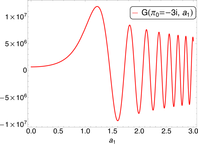
Figure 1: We consider the boundary conditions motivated by no-boundary Universe which imply $\pi_{0}=-3i$. Here we choose parameter values: $k=1$, $\Lambda=3$, and $\alpha=2$. Here we plot the exact transition amplitude $G(\pi_{0}=-3i,a_{1})$ given in eq. (54) as $a_{1}=\sqrt{q_{1}}$ is varied from $0$ to larger values.

The asymptotic expressions for the two Airy functions are: $Ai(z)\sim\exp(-2z^{3/2}/3)$ and $Bi(z)\sim\exp(2z^{3/2}/3)$. This immediately tell us that the relevant Airy-function that we seek is $Bi(z)$ as that is the one which grows large when $z$ becomes large. This will imply that for $\Lambda<0$ we have

$$\biggl{.}\Psi_{2}(q_{1})\biggr{|}_{\Lambda<0}=\left(\frac{24\pi G\hbar}{V_{3}\Lambda^{2}}\right)^{1/3}Bi\left[\left(\frac{\sqrt{3}V_{3}}{-8\pi G\hbar\Lambda}\right)^{2/3}\left(3k-\Lambda q_{1}\right)\right]\,,$$ (50)

where we have reinstated factors of $V_{3}$ and $G$ in the above. Now to obtain the expression for the case of $\Lambda>0$ we can do an analytic continuation by making use of the following identity relating the Airy-functions $Ai(z)$ and $Bi(z)$

$$Bi(z)=i\omega Ai(\omega z)-i\omega^{2}Ai(\omega^{2}z)\,,$$ (51)

where $\omega=e^{i2\pi/3}$ is the cube-root of unity.

This means that in our case the two Airy functions satisfy the following relation

$$Bi\left[\left(\frac{\sqrt{3}V_{3}}{-8\pi G\hbar\Lambda}\right)^{2/3}\left(3k-\Lambda q_{1}\right)\right] =e^{i\pi/6}Ai\left[e^{i2\pi/3}\left(\frac{\sqrt{3}V_{3}}{-8\pi G\hbar\Lambda}\right)^{2/3}\left(3k-\Lambda q_{1}\right)\right]$$ (52)

$$+e^{-\pi/6}Ai\left[e^{-i2\pi/3}\left(\frac{\sqrt{3}V_{3}}{-8\pi G\hbar\Lambda}\right)^{2/3}\left(3k-\Lambda q_{1}\right)\right]$$

$$=\sqrt{3}Ai\left[\left(\frac{\sqrt{3}V_{3}}{8\pi G\hbar\Lambda}\right)^{2/3}\left(3k-\Lambda q_{1}\right)\right]\,.$$

We notice that for $\Lambda>0$ the function $\Psi_{2}(q_{1})$ is given by

$$\biggl{.}\Psi_{2}(q_{1})\biggr{|}_{\Lambda>0}=\sqrt{3}\left(\frac{24\pi G\hbar}{V_{3}\Lambda^{2}}\right)^{1/3}Ai\left[\left(\frac{\sqrt{3}V_{3}}{8\pi G\hbar\Lambda}\right)^{2/3}\left(3k-\Lambda q_{1}\right)\right]\,,$$ (53)

which is real. If we combine this with the expression for $\Psi_{1}(\pi_{0})$ then we get the full expression for the transition amplitude

$$\biggl{.}G[{\rm bd}_{0},{\rm bd}_{1}]\biggr{|}_{\Lambda>0}= \sqrt{\frac{3}{\pi i}}\left(\frac{3\pi G\hbar}{V_{3}\Lambda^{2}}\right)^{1/3}\exp\left[\frac{iV_{3}}{8\pi G\hbar}\left(\frac{3}{\Lambda}+4\alpha\right)\left(k\pi_{0}+\frac{\pi_{0}^{3}}{27}\right)\right]$$ (54)

$$\times Ai\left[\left(\frac{\sqrt{3}V_{3}}{8\pi G\hbar\Lambda}\right)^{2/3}\left(3k-\Lambda q_{1}\right)\right]\,.$$

This is an exact result for the transition amplitude for the $\Lambda>0$ in the case when Neumann boundary conditions are imposed at initial boundary and Dirichlet boundary conditions are imposed on final boundary. Notice also the non-trivial correction coming from the Gauss-Bonnet coupling in the exponential factor. This GB-correction however doesn’t appear in the argument of the Airy-function, which is also independent of initial momentum $\pi_{0}$.

Notice that so far we haven’t assumed any special value for $\pi_{0}$, which is chosen by demanding the geometry to be non-singular at an initial time and fluctuations to be well-behaved. For $k=1$ if $\pi_{0}$ is such that ${\rm Im}[\pi_{0}(1+\pi_{0}^{2}/27)]>0$ then it will lead to an exponential with positive real part, and negative otherwise. In the next section we will see there is one such $\pi_{0}$ which fits these criterion and is favourable.

In figure 1 we plot the exact transition amplitude for a certain choice of parameter values. It is easy to notice its characteristic features: namely it rises exponentially from $q_{1}=0$ (note that value of amplitude at $q_{1}=0$ is non-zero) to $q_{1}=3k/\Lambda$ after which it starts to oscillate with increasing frequency but with diminishing amplitude. In the next section we will study the saddle-point picture to better understand the behaviour of the transition amplitude.

VII Saddle-point approximation

The lapse integration mentioned in eq. (42) can also be studied using Picard-Lefschtez technology and evaluating it in the saddle-point approximation. Although it doesn’t provide us with an exact result but saddle-point analysis helps us in understanding the behaviour of transition amplitude as $q_{1}$ increases (see Feldbrugge:2017kzv ; Narain:2021bff ; Witten:2010cx ; Witten:2010zr ; Basar:2013eka ; Tanizaki:2014xba for review on Picard-Lefschtez and analytic continuation).

We start by first studying the action in eq. (34) and computing the saddle points for the lapse $N_{c}$. These can be determined by computing the quantity $dS_{\rm tot}/dN_{c}$. These saddle points can be obtained by solving the equation

$$\frac{{\rm d}S_{\rm tot}}{{\rm d}N_{c}}=\frac{\Lambda^{2}}{3}N_{c}^{2}-\frac{2\Lambda\pi_{0}}{3}N_{c}+3k-\Lambda q_{1}+\frac{\pi_{0}^{2}}{3}=0\,.$$ (55)

This is a quadratic equation in $N_{c}$ resulting in two saddle points. The discriminant $\Delta$ for the above equation is given by

$$\Delta=4\Lambda^{2}\left(\frac{\Lambda q_{1}}{3}-k\right)\,.$$ (56)

It is crucial to note here that for $\Lambda>0$ (dS geometry) the discriminant $\Delta$ can change sign depending on the value of $q_{1}$ (size determining the outer boundary). This will result in stokes phenomena as will be seen later (in the case of AdS-geometry $\Lambda<0$ sign of $\Delta$ never changes). The two saddle points are then given by

$$N_{\pm}=\frac{3}{\Lambda}\left[\frac{\pi_{0}}{3}\pm\left(\frac{\Lambda q_{1}}{3}-k\right)^{1/2}\right]\,.$$ (57)

It is worthwhile to remark here that as expected these saddles don’t depend GB coupling $\alpha$ for the case of NBC. The action at these saddle points becomes the following

$$S_{\rm tot}(N_{\pm})=\pm\frac{6}{\Lambda}\left(\frac{\Lambda q_{1}}{3}-k\right)^{3/2}+\left(\frac{3}{\Lambda}+4\alpha\right)\left(k\pi_{0}+\frac{\pi_{0}^{3}}{27}\right)\,.$$ (58)

Notice that the change of variable mentioned in eq. (43) will imply that the saddle points for the shifted lapse $\bar{N}$ are given by,

$$\bar{N}_{\pm}=\pm\frac{3}{\Lambda}\left(\frac{\Lambda q_{1}}{3}-k\right)^{1/2}\,.$$ (59)

Now there are two possibilities: $q_{1}>3k/\Lambda$ and $q_{1}<3k/\Lambda$. In the former case ($q_{1}>3k/\Lambda$) the saddle points given in eq. (59) lie on real axis ($\bar{N}_{+}$ on positive real axis and $\bar{N}_{-}$ on negative real axis). In the case when $q_{1}<3k/\Lambda$ the saddle points are both imaginary with one lying on positive imaginary axis while the other lying on negative imaginary axis. The case when $q_{1}=3k/\Lambda$ is degenerate when both saddle points are located at $\bar{N}_{\pm}=0$. These three cases have been studied in detail in Lehners:2021jmv for the case of Einstein-Hilbert gravity. In our study we notice that the presence of Gauss-Bonnet coupling gives an additional contribution but doesn’t change the overall qualitative picture as far as saddle-point analysis is concerned.

We will now make a particular choice for the initial momentum $\pi_{0}$ using which will proceed with the saddle-point analysis to gain more insight of the nature of transition amplitude and the evolution of Universe. To do this we take inspiration from no-boundary Universe where the intuitive understanding is that the geometry gets rounded off at beginning of time. This means that if we write $\Lambda=3\lambda^{2}>0$ in $d=4$ then we have for the Lorentzian spacetime dS metric in eq. (2)

$$N_{p}=1\,,\hskip 14.22636pta(t_{p})=\frac{1}{\lambda}\cosh\left(\lambda t_{p}\right)\,.$$ (60)

deSitter geometry when embedded in $5$-dimensions then in closed slicing it can pictured as hyperboloid having a minimum spatial extent at $t_{p}=0$. Now the rounding off the geometry is achievable by analytically continuing the original dS-metric to Euclidean time, starting exactly at the waist of hyperboloid at $t_{p}=0$. This means

$$t_{p}=\mp i\left(\tau-\frac{\pi}{2\lambda}\right)\,,\hskip 14.22636pt0\leq\tau\leq\frac{\pi}{2\lambda}\,.$$ (61)

This means that along the Euclidean section the dS metric transforms in to that of a $4$-sphere

$${\rm d}s^{2}={\rm d}\tau^{2}+\frac{1}{\lambda^{2}}\sin^{2}\left(\lambda\tau\right){\rm d}\Omega_{3}^{2}\,.$$ (62)

This geometry has no boundary at $\tau=0$ and smoothly closes off.

Now there are two possibilities of the time rotation to the above Euclidean time. Each corresponding to the sign appearing in eq. (61) and each leading to a different Wick rotation. The upper sign which is also used in the standard Wick rotation in the flat spacetime QFT, is also the sign chosen in the works of Hartle and Hawking Hartle:1983ai ; Halliwell:1984eu . In this sign choice perturbations are stable and suppressed. The lower sign in eq. (61) however correspond to Vilenkin’s tunneling geometry in which perturbation are unsuppressed Feldbrugge:2017fcc ; Halliwell:1989dy . The Wick rotation process here can also be thought of as the lapse $N_{p}$ changing its value from $N_{p}=1$ to $N_{p}=\mp i$, thereby implying that the total time $T_{p}=\int N_{p}{\rm d}t_{p}$ becoming complex valued.

This when translated in language of metric given in eq. (16) will imply

$$\sinh\left(\lambda t_{p}\right)=\lambda^{2}N_{\rm HH}t+i\,,$$ (63)

where $N_{\rm HH}$ will turn out to be the saddle-point value of of the lapse corresponding to Hartle-Hawking geometry Hartle:1983ai ; Halliwell:1984eu . It is given by

$$N_{\rm HH}=\frac{\sqrt{\lambda^{2}q_{1}-1}}{\lambda^{2}}-\frac{i}{\lambda^{2}}\,,$$ (64)

If we compare this with the saddle point values mentioned in eq. (57) then for our case this will imply that for the no-boundary Universe one has

$$\left.\pi_{0}\right|_{\rm Hartle-Hawking\,\,(HH)}=-3i\,.$$ (65)

For this value of $\pi_{0}$ the initial geometry is smoothly rounded-off and is non-singular. Moreover for this value the fluctuations are also well-behaved around the saddle points and are suppressed. In the following we will assume this particular value for $\pi_{0}$ to proceed with the saddle-point analysis. In this case it is noticed that when this value of $\pi_{0}$ is plugged into the lapse action given in eq. (34) then the action becomes complex. This complex acton is given by

$$S_{\rm tot}^{\rm HH}=\frac{\Lambda^{2}}{9}N_{c}^{3}+i\Lambda N_{c}^{2}-\Lambda q_{1}N_{c}-3iq_{1}-8\alpha i\,,$$ (66)

while the action at the two saddle-points $N_{\pm}^{HH}$ is given by

$$S^{\rm HH}_{\pm}=\pm\frac{6}{\Lambda}\left(\frac{\Lambda q_{1}}{3}-1\right)^{3/2}-2i\left(\frac{3}{\Lambda}+4\alpha\right)\,.$$ (67)

We can also compute the second-derivative of the lapse-action at the saddle-points and this is given by

$$\biggl{.}\frac{{\rm d}^{2}S}{{\rm d}N_{c}}\biggr{|}_{N_{c}=N_{\pm}}=\pm 2\Lambda\sqrt{\frac{q_{1}\Lambda}{3}-k}\,.$$ (68)

It should be mentioned that the second-derivative is independent of initial momentum $\pi_{0}$, and that the saddle-point approximation will work as long as ${\rm d}^{2}S/{\rm d}N_{c}$ don’t vanish for some value $q_{1}$. The complex action in eq. (66) is a direct consequence of imposing complex initial momentum, which subsequently leads to complex geometries. A complex action will imply that even for geometries with real lapse $N_{c}$ there will be a a non-zero weighting corresponding to them.

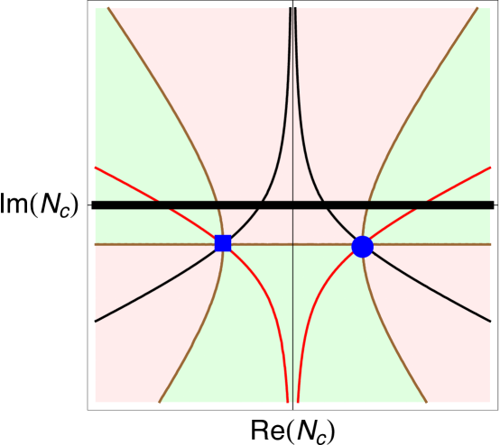
Figure 2: We consider the case of no-boundary Universe where we impose the mixed boundary condition: with Euclidean momentum at $t=0$ and fixed final size at $t=1$. The lapse action given in eq. (34) is complex. We take $\pi_{0}=-3i$ motivated by works of Hartle & Hawking Hartle:1983ai ; Halliwell:1984eu . For the purpose of this numerical example we have set $\Lambda=3$, $\alpha=2$ and $q_{1}=3$. We plot on $x$-axis real-part of $N_{c}$ while the $y$-axis is imaginary part of $N_{c}$. The red lines correspond to steepest descent lines (thimbles ${\cal J}_{\sigma}$), while the thin black lines are steepest ascent lines and denoted by ${\cal K}_{\sigma}$. Both the saddle points are depicted in blue: $N_{-}$ (blue-square) and $N_{+}$ (blue-circle). Both saddle points are relevant. The steepest ascent lines emanating from both of them intersects the original integration contour $(-\infty,+\infty)$ which is shown by thick-black line. The Morse-function $h$ is same for both saddle points: $h(N_{\pm})>0$. The light-green region is allowed region with $h<h(N_{\sigma})$ for all values of $\sigma$. The light-pink region (forbidden region) has $h>h(N_{\sigma})$ for all $\sigma$. The boundary of these region is depicted in brown lines. Along these line we have $h=h(N_{\sigma})$.

At this point our interest turns to compute transition amplitude given in eq. (42) by using Picard-Lefschetz technology and employing saddle-point approximation. Once the saddle points are known, one can compute the steepest ascent/descent flow lines corresponding to each of the saddle point. A relevant saddle point is one if the steepest ascent path emanating from it hits the original integration contour which is $(-\infty,+\infty)$. For real action it implies that relevant saddle points will have a negative-valued Morse-function. However, when action is complex then this is no longer true DiTucci:2019bui ; Narain:2021bff ; Lehners:2021jmv ; DiTucci:2020weq .

VII.1 $q_{1}>3/\Lambda$

It should be noticed that for $q_{1}>3/\Lambda$ the Morse-function

$$h(N^{\rm HH}_{\pm})=\frac{2}{\hbar}\left(\frac{3}{\Lambda}+4\alpha\right)\,.$$ (69)

It is real, positive and independent of $q_{1}$. Both saddle points are relevant even though for both of them $h(N_{\pm})>0$. In figure 2 we plot the various flow-line, saddle points, forbidden/allowed regions. As both saddle points are relevant so the Lefschetz thimbles passing through them constitute the deformed contour of integration. The Picard-Lefschetz theory then gives the transition amplitude in the saddle point approximation as

$$G[\pi_{0}=-3i,q_{1}>\frac{3}{\Lambda}]\approx\frac{(q_{1}\Lambda/3-1)^{-1/4}}{2\sqrt{2\Lambda\pi i}}\left[e^{i\pi/4}\exp\left(\frac{iS^{\rm HH}_{\rm tot}(N_{+})}{\hbar}\right)-e^{-i\pi/4}\exp\left(\frac{iS^{\rm HH}_{\rm tot}(N_{-})}{\hbar}\right)\right]$$

$$=\frac{e^{-i\pi/4}}{(q_{1}\Lambda/3-1)^{1/4}\sqrt{2\Lambda\pi}}\exp\left[\frac{V_{3}}{4\pi G\hbar}\left(\frac{3}{\Lambda}+4\alpha\right)\right]\sin\left[\frac{3V_{3}}{2\pi G\Lambda\hbar}\left(\frac{\Lambda q_{1}}{3}-1\right)^{3/2}+\frac{\pi}{4}\right]\,,$$ (70)

where in the last line we have reinstated factors of $V_{3}$ and $G$. The transition amplitude oscillates ever faster with increasing $q_{1}$ while its weighting remains constant. This implies that the system becomes classical in the WKB sense. Therefore, successive path integrals with increasing real boundary values for $q_{1}$ describe real Lorentzian deSitter universes (even though the saddle points in each individual path integral have a complex geometry), as long as $q_{1}>3/\Lambda$.

VII.2 $q_{1}<3/\Lambda$

In this case the discriminant given in eq. (56) is negative, implying that the term $\left(\Lambda q_{1}/3-k\right)^{1/2}$ will become imaginary. This will mean that the saddle point geometries are completely Euclidean in nature. The action at the saddle points will get an additional imaginary contribution for $\pi_{0}=-3i$. In this case we notice that the Morse-function $h$ at the saddle points changes and is given by

$$h(N^{\rm HH}_{\pm})=\pm\frac{6}{\Lambda\hbar}\left(1-\frac{\Lambda q_{1}}{3}\right)^{3/2}+\frac{2}{\hbar}\left(\frac{3}{\Lambda}+4\alpha\right)$$ (71)

We therefore realize that only the saddle point $N_{-}$ is relevant. This mean that the transition amplitude for $q_{1}<3/\Lambda$ is given by

$$G[\pi_{0}=-3i,q_{1}<\frac{3}{\Lambda}]\approx\frac{(1-q_{1}\Lambda/3)^{-1/4}}{2\sqrt{2\Lambda\pi i}}e^{i3\pi/2}\exp\left(\frac{iS^{\rm HH}_{\rm tot}(N_{-})}{\hbar}\right)$$

$$=\frac{e^{-i\pi/2}}{(1-q_{1}\Lambda/3)^{1/4}\sqrt{2\Lambda\pi}}\exp\left[-\frac{3V_{3}}{4\pi G\hbar\Lambda}\left(1-\frac{\Lambda q_{1}}{3}\right)^{3/2}\right]\exp\left[\frac{V_{3}}{4\pi G\hbar}\left(\frac{3}{\Lambda}+4\alpha\right)\right]\,,$$ (72)

where in the last line we have reinstated factors of $V_{3}$ and $G$. This agrees with the result obtained in Lehners:2021jmv for $\alpha=0$ case. This also shows that for $q_{1}<3/\Lambda$ the Universe is in Euclidean phase.

VII.3 $q_{1}=3/\Lambda$

This is a degenerate situation when $\Delta=0$. In this case both the saddle points are same $\bar{N}_{\pm}=0$. The saddle point action is purely imaginary given by

$$S^{\rm HH}_{\pm}(q_{1}=\frac{3}{\Lambda})=-2i\left(\frac{3}{\Lambda}+4\alpha\right)\,,$$ (73)

while the Morse-function is given in eq. (69).

In this degenerate case the saddle point approximation breaks-down as the double-derivative of the lapse action given in eq.(68) computed at the saddle-points vanishes. This means that one can’t perform the lapse integration for this degenerate case using saddle-point approximation. This is a short coming in the saddle point approximation as it cannot be applied in such situations. This breakdown of the saddle-point approximation will not depend on the value of $\pi_{0}$. In such a situation one has to look beyond saddle-point approximation. The exact result computed in section VI and mentioned in eq. (54) doesn’t have this problem and gives a reliable result.

VIII Initial condition independence

An interesting feature that is noticed in the above computations is the appearance of a hypothetical situation when some of the couplings of the gravitational theory that is mentioned in eq. (1) have a particular relation. It is seen that if incase there is a situation when

$$\alpha=-\frac{3}{4\Lambda}\,$$ (74)

then the exponential factor appearing in the exact result for the transition amplitude given in eq. (54) becomes unity as the corresponding argument of the exponential function vanishes. This happens irrespective of the value of $\pi_{0}$, although this doesn’t mean that the initial momentum $\pi_{0}$ is arbitrary.

In the case of saddle-point approximation we notice that when $\alpha$ and $\Lambda$ satisfy the relation given in eq. (74) then for $q_{1}>3/\Lambda$ the Morse-function given in eq. (69) vanishes. While for $q_{1}<3/\Lambda$ the Morse-function given in eq. (71) is left with the part dependent only on $q_{1}$. In both the cases however the second-derivative of lapse action given in eq. (68) remains independent of $\pi_{0}$ (this is irrespective of the relationship between $\alpha$ and $\Lambda$). In both these cases the saddle-point approximation will hold as the second-derivative of action at the saddle-point don’t vanish. However, in both these cases we notice that the exponential appearing in the transition amplitude in eq. (VII.1 and VII.2) becomes unity, as once again the corresponding argument of the exponential factors vanishes.

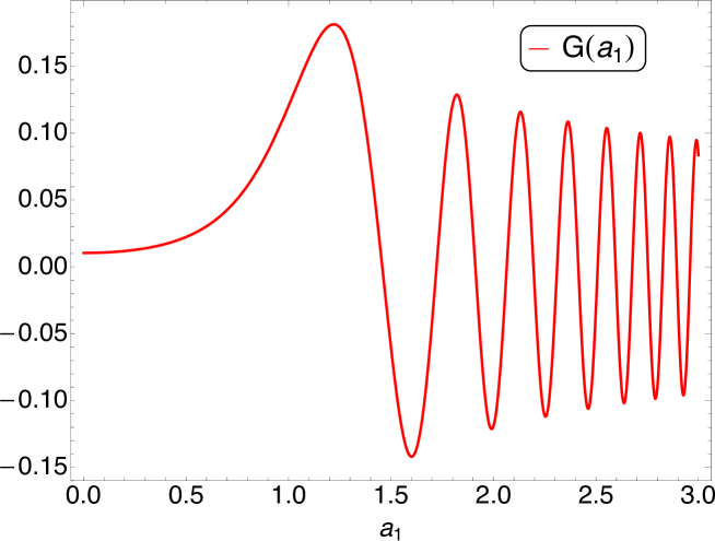
Figure 3: Here we choose parameter values: $k=1$, $\Lambda=3$, and $\alpha=-\frac{3}{4\Lambda}$. Here we plot the exact transition amplitude $G(a_{1})$ given in eq. (VIII) as $a_{1}=\sqrt{q_{1}}$ is varied from $0$ to larger values.

It implies that when $\alpha$ and $\Lambda$ satisfy the relation in eq. (74) then we have

$$\Psi_{1}(\pi_{0})=\frac{1}{\sqrt{\pi i}}\,.$$ (75)

At this special value of GB-coupling the dependence on the initial momentum $\pi_{0}$ disappears completely (also note that we haven’t fix the initial size $q_{0}$ of the Universe as we were considering Neumann boundary conditions at the initial boundary). So for this special case the exact transition amplitude (or the wave-function of Universe) is given by

$$\biggl{.}G[{\rm bd}_{1}]\biggr{|}_{\Lambda>0}= \frac{1}{\sqrt{\pi i}}\Psi_{2}(q_{1})$$

$$= \sqrt{\frac{3}{\pi i}}\left(\frac{3\pi G\hbar}{V_{3}\Lambda^{2}}\right)^{1/3}Ai\left[\left(\frac{\sqrt{3V_{3}}}{8\pi G\hbar\Lambda}\right)^{2/3}\left(3k-\Lambda q_{1}\right)\right]\,.$$ (76)

This is independent of both the initial size $a_{0}=\sqrt{q_{0}}$ (which is arbitrary as we imposing Neumann boundary conditions) and initial momentum $\pi_{0}$ (which is fixed to some value). It only depends on the final size of the Universe which is given by $a_{1}=\sqrt{q_{1}}$. In figure 3 we plot this transition amplitude as as function of final size of Universe given by scale-factor $a_{1}=\sqrt{q_{1}}$. The qualitative behaviour of transition amplitude as seen from figure 3 is same as before. For $q_{1}<3/\Lambda$ the wavefunction grows exponentially indicating a Euclidean phase of Universe when there is no notion of time. Note that the value of $G(a_{1})$ at $a_{1}=0$ is non-zero although small. The wave-function reaches a peak value at $q_{1}=3/\Lambda$ and thereafter it has a oscillatory feature with diminishing amplitude. This is Lorentzian phase of the Universe where emergence of the time has occurred. The system becomes classical in the WKB sense.

This hypothetical situation of independence from initial condition doesn’t happen in EH gravity without Gauss-Bonnet modification ($\alpha=0$ case). In the case of Gauss-Bonnet gravity the generation of extra terms allows for the possibility where terms cancel out. However, it is important to point out that this independence doesn’t imply that $\pi_{0}$ is arbitrary. The initial momentum $\pi_{0}$ is fixed to some value which is chosen by requiring that the geometry is smoothly rounded-off at in initial time and perturbations are suppressed. Still it is interesting to note that the dependence on $\pi_{0}$ disappears completely in the transition amplitude for this hypothetical scenario, although regularity and stability requirements picks up a value for $\pi_{0}$.

We call this situation ‘initial condition independence’ in a loose sense as the wave-function becomes independent of the initial boundary configuration: initial size $q_{0}$ (which is arbitrary) and initial momentum $\pi_{0}$ (which is fixed in such a way so to avoid initial singularity and in which perturbations around the saddle-points are suppressed). It should be mentioned that for this particular value of $\alpha$ given in eq. (74) our original action mentioned in eq. (1) acquires a MacDowell-Mansouri form MacDowell:1977jt in four dimensions

$$S=-\frac{1}{256\pi G}\int{\rm d}^{4}x\sqrt{-g}\delta^{[\sigma\lambda\mu\nu]}_{[\gamma\delta\alpha\beta]}\biggl{(}\sqrt{\frac{3}{\Lambda}}R^{\gamma\delta}{}_{\sigma\lambda}-\sqrt{\frac{\Lambda}{3}}\delta^{[\gamma\delta]}_{[\sigma\lambda]}\biggr{)}\biggl{(}\sqrt{\frac{3}{\Lambda}}R^{\alpha\beta}{}_{\mu\nu}-\sqrt{\frac{\Lambda}{3}}\delta^{[\alpha\beta]}_{[\mu\nu]}\biggr{)}\,.$$ (77)

Interestingly for this same value of $\alpha$ one also obtains finite Noether charges Miskovic:2006tm (see Miskovic:2009bm for topological regularization). This special value of $\alpha=-3/4\Lambda$ is therefore has significance.

IX Conclusions

In this paper we studied the path-integral of the Gauss-Bonnet gravity in four spacetime dimensions directly in Lorentzian signature. In four spacetime dimensions the Gauss-Bonnet sector of gravity is topological in nature and doesn’t contribute in the bulk dynamics. However, it has an important role to play at the boundaries. Depending on the nature of boundary conditions the Gauss-Bonnet modifications will affect the study of path-integral as has also been noticed in an earlier work Narain:2021bff . This paper aims to investigate these issues in more detail by considering the gravitational path-integral in a reduced setup of mini-superspace approximation.

We start with the mini-superspace action of the theory and vary it with respect to the field. This will tell us the dynamical equation of motion and nature of the boundary terms. For a consistent variational problem one has to incorporate suitable boundary terms. In principle the boundary configurations are chosen in such a way so that the variational problem leading to the equation of motion (and its solution) is consistent, but it is important (and actually better) to choses those BC which leads to stable perturbations around the saddle points. In these situations the path-integral then reduces to a summation over all the stable geometries, where boundary configurations leading to unstable saddles are not incorporated. It is a kind of stability condition.

We study the system with mixed boundary conditions: imposing Neumann boundary conditions on the initial boundary and imposing Dirichlet boundary condition on the final boundary. Motivation for studying mixed boundary conditions stems from various past works: as the Gauss-Bonnet sector of gravity contributes non-trivially Narain:2021bff , and imposing Neumann BC on the initial boundary is seen to lead to saddles where fluctuations are suppressed DiTucci:2019bui ; Narain:2021bff ; Lehners:2021jmv ; DiTucci:2020weq . These studies show the importance of using Neumann (or Robin) BC at the initial boundary. They also further support the situation when Neumann BC is imposed at initial boundary while a Dirichlet BC is imposed at final boundary DiTucci:2019bui ; Narain:2021bff ; DiTucci:2020weq ; Lehners:2021jmv , as the perturbations are suppressed.

In such a scenario we study the path-integral of Gauss-Bonnet gravity in mini-superspace approximation, and compute the transition amplitude from one $3$-geometry to another. This is given by a path-integral over $q(t)$ and a contour integration over lapse $N_{c}$. The path-integral over $q(t)$ can be performed exactly as the Gauss-Bonnet part only gives some boundary contributions. Once this is performed we are left with a contour integration over the lapse $N_{c}$ whose action is given by eq. (34).

To deal with the lapse integration we do a change of variable and shift the lapse by a constant. This allows us to cancel some terms in the lapse-action while pushing all the dependence on the initial momentum $\pi_{0}$ in a constant peice. This step simplifies the expression for transition amplitude as it gets factored into two parts: one entirely dependent on the initial momentum $\pi_{0}$ and another which is entirely a function of final size of Universe $q_{1}$. We name these two factors $\Psi_{1}(\pi_{0})$ and $\Psi_{2}(q_{1})$ respectively. The function $\Psi_{2}(q_{1})$ is a contour integral over shifted-lapse which can be recognized as an Airy-integral. This can be performed exactly. We compute this first in AdS-geometry $\Lambda<0$ (as the argument of the function is positive), then analytically continue to the case of dS-geometry ($\Lambda>0$) in which we are interested. Combining the expression for $\Psi_{1}$ and $\Psi_{2}$ gives an exact result for the transition amplitude in four spacetime dimensions for the case of Gauss-Bonnet gravity in mini-superspace approximation.

We then study the transition amplitude given as a lapse integral in eq. (42) in the saddle point approximation. We do this to gain more insight in to the behaviour and nature of various complex-saddle points as the size of Universe $a_{1}=\sqrt{q_{1}}$ increases. We take inspiration from the no-boundary proposal of Universe where the spacetime geometry at initial time is smoothly rounded-off. This aids us in making an educated guess for the initial momentum $\pi_{0}$, which is the value also considered by Hartle-Hawking in their past studies and which is known to lead to stable perturbations around relevant saddle point. For this choice of $\pi_{0}$ in the saddle point approximation we notice that for $q_{1}<3/\Lambda$ the saddle-point geometry is Euclidean and that the transition amplitude is governed by the Euclidean saddle-point. While for $q_{1}>3/\Lambda$ the saddle-point consists of complex conjugate pair and both complex-saddles contribute to transition amplitude leading to oscillations.

We come across an interesting hypothetical situation when the cosmological constant $\Lambda$ and Gauss-Bonnet coupling $\alpha$ are related as in eq. (74). In this case the transition amplitude becomes independent of the initial momentum $\pi_{0}$. As the initial size of Universe ($q_{0}$) was left unspecified, so the transition amplitude is completely independent of initial size $q_{0}$ (which is left arbitrary as we are imposing Neumann boundary conditions at the initial boundary) and initial momentum $\pi_{0}$. Although the dependence on initial momentum disappears from the wave-function, but it should be mentioned that the initial momentum is not left arbitrary. It needs to be fixed to a value which is chosen based on regularity and stability requirements. It is still interesting to note that for this special value $\alpha=-3/4\Lambda$, the dependence on conjugate momentum $\pi_{0}$ disappears from the wave-function. We call this hypothetical situation initial-condition independence in a loose sense.

This hypothetical situation of the wave-function being independent of the initial boundary values don’t arise in Einstein-Hilbert gravity without Gauss-bonnet (GB) modification and/or when the GB-coupling don’t take such a special value. The current works shows the non-trivial contributions that arises from the Guass-Bonnet terms in the gravitational action when one studies the no-boundary proposal of Universe. Furthermore, it highlights the importance of a particular special value of $\alpha$ when the wave-function of the no-boundary Universe will enjoy an additional independence from initial boundary values, something which was not witnessed before. Interestingly for this special value of $\alpha$ the original gravitational action acquires a MacDowell-Mansouri form, and has separately been observed to lead to finite Noether charges Miskovic:2006tm . It would be worth exploring such connections in more detail in future.

Acknowledgements

I am thankful to Jean-Luc Lehners and Nirmalya Kajuri for useful discussions. I am thankful to BJUT for kind hospitality and support during the course of this work.

References

- (1) G. ’t Hooft and M. J. G. Veltman, “One loop divergencies in the theory of gravitation,” Ann. Inst. H. Poincare Phys. Theor. A 20, 69-94 (1974)
- (2) S. Deser, H. S. Tsao and P. van Nieuwenhuizen, “Nonrenormalizability of Einstein Yang-Mills Interactions at the One Loop Level,” Phys. Lett. B 50, 491-493 (1974) doi:10.1016/0370-2693(74)90268-8
- (3) S. Deser and P. van Nieuwenhuizen, “One Loop Divergences of Quantized Einstein-Maxwell Fields,” Phys. Rev. D 10, 401 (1974) doi:10.1103/PhysRevD.10.401
- (4) S. Deser and P. van Nieuwenhuizen, “Nonrenormalizability of the Quantized Dirac-Einstein System,” Phys. Rev. D 10, 411 (1974) doi:10.1103/PhysRevD.10.411
- (5) M. H. Goroff and A. Sagnotti, “QUANTUM GRAVITY AT TWO LOOPS,” Phys. Lett. B 160, 81-86 (1985) doi:10.1016/0370-2693(85)91470-4
- (6) M. H. Goroff and A. Sagnotti, “The Ultraviolet Behavior of Einstein Gravity,” Nucl. Phys. B 266, 709-736 (1986) doi:10.1016/0550-3213(86)90193-8
- (7) A. E. M. van de Ven, “Two loop quantum gravity,” Nucl. Phys. B 378, 309-366 (1992) doi:10.1016/0550-3213(92)90011-Y
- (8) K. S. Stelle, “Renormalization of Higher Derivative Quantum Gravity,” Phys. Rev. D 16, 953-969 (1977) doi:10.1103/PhysRevD.16.953
- (9) A. Salam and J. A. Strathdee, “Remarks on High-energy Stability and Renormalizability of Gravity Theory,” Phys. Rev. D 18, 4480 (1978) doi:10.1103/PhysRevD.18.4480
- (10) J. Julve and M. Tonin, “Quantum Gravity with Higher Derivative Terms,” Nuovo Cim. B 46, 137-152 (1978) doi:10.1007/BF02748637
- (11) E. S. Fradkin and A. A. Tseytlin, “Renormalizable asymptotically free quantum theory of gravity,” Nucl. Phys. B 201, 469-491 (1982) doi:10.1016/0550-3213(82)90444-8
- (12) I. G. Avramidi and A. O. Barvinsky, “ASYMPTOTIC FREEDOM IN HIGHER DERIVATIVE QUANTUM GRAVITY,” Phys. Lett. B 159, 269-274 (1985) doi:10.1016/0370-2693(85)90248-5
- (13) I. L. Buchbinder, S. D. Odintsov and I. L. Shapiro, “Effective action in quantum gravity,”
- (14) G. Narain and R. Anishetty, “Short Distance Freedom of Quantum Gravity,” Phys. Lett. B 711, 128-131 (2012) doi:10.1016/j.physletb.2012.03.070 [arXiv:1109.3981 [hep-th]].
- (15) G. Narain and R. Anishetty, “Unitary and Renormalizable Theory of Higher Derivative Gravity,” J. Phys. Conf. Ser. 405, 012024 (2012) doi:10.1088/1742-6596/405/1/012024 [arXiv:1210.0513 [hep-th]].
- (16) G. Narain, “Signs and Stability in Higher-Derivative Gravity,” Int. J. Mod. Phys. A 33, no.04, 1850031 (2018) doi:10.1142/S0217751X18500318 [arXiv:1704.05031 [hep-th]].
- (17) G. Narain, “Exorcising Ghosts in Induced Gravity,” Eur. Phys. J. C 77, no.10, 683 (2017) doi:10.1140/epjc/s10052-017-5249-z [arXiv:1612.04930 [hep-th]].
- (18) A. Codello and R. Percacci, “Fixed points of higher derivative gravity,” Phys. Rev. Lett. 97, 221301 (2006) doi:10.1103/PhysRevLett.97.221301 [arXiv:hep-th/0607128 [hep-th]].
- (19) M. R. Niedermaier, “Gravitational Fixed Points from Perturbation Theory,” Phys. Rev. Lett. 103, 101303 (2009) doi:10.1103/PhysRevLett.103.101303
- (20) A. Salvio and A. Strumia, “Agravity,” JHEP 06, 080 (2014) doi:10.1007/JHEP06(2014)080 [arXiv:1403.4226 [hep-ph]].
- (21) D. Lovelock, “The Einstein tensor and its generalizations,” J. Math. Phys. 12, 498-501 (1971) doi:10.1063/1.1665613
- (22) D. Lovelock, “The four-dimensionality of space and the einstein tensor,” J. Math. Phys. 13, 874-876 (1972) doi:10.1063/1.1666069
- (23) C. Lanczos, “A Remarkable property of the Riemann-Christoffel tensor in four dimensions,” Annals Math. 39, 842-850 (1938) doi:10.2307/1968467
- (24) B. Zwiebach, “Curvature Squared Terms and String Theories,” Phys. Lett. B 156, 315-317 (1985) doi:10.1016/0370-2693(85)91616-8
- (25) D. J. Gross and J. H. Sloan, “The Quartic Effective Action for the Heterotic String,” Nucl. Phys. B 291, 41-89 (1987) doi:10.1016/0550-3213(87)90465-2
- (26) R. R. Metsaev and A. A. Tseytlin, “Order alpha-prime (Two Loop) Equivalence of the String Equations of Motion and the Sigma Model Weyl Invariance Conditions: Dependence on the Dilaton and the Antisymmetric Tensor,” Nucl. Phys. B 293, 385-419 (1987) doi:10.1016/0550-3213(87)90077-0
- (27) K. Chakravarti, R. Ghosh and S. Sarkar, “Bounding the Boundless: Constraining Topological Gauss-Bonnet Coupling from GW150914,” [arXiv:2201.08700 [gr-qc]].
- (28) M. Isi, W. M. Farr, M. Giesler, M. A. Scheel and S. A. Teukolsky, “Testing the Black-Hole Area Law with GW150914,” Phys. Rev. Lett. 127, no.1, 011103 (2021) doi:10.1103/PhysRevLett.127.011103 [arXiv:2012.04486 [gr-qc]].
- (29) I. A. Batalin and G. A. Vilkovisky, “Relativistic S Matrix of Dynamical Systems with Boson and Fermion Constraints,” Phys. Lett. B 69, 309-312 (1977) doi:10.1016/0370-2693(77)90553-6
- (30) C. Teitelboim, “Quantum Mechanics of the Gravitational Field,” Phys. Rev. D 25, 3159 (1982) doi:10.1103/PhysRevD.25.3159
- (31) C. Teitelboim, “The Proper Time Gauge in Quantum Theory of Gravitation,” Phys. Rev. D 28, 297 (1983) doi:10.1103/PhysRevD.28.297
- (32) J. J. Halliwell, “Derivation of the Wheeler-De Witt Equation from a Path Integral for Minisuperspace Models,” Phys. Rev. D 38, 2468 (1988) doi:10.1103/PhysRevD.38.2468
- (33) C. Teitelboim, “Causality Versus Gauge Invariance in Quantum Gravity and Supergravity,” Phys. Rev. Lett. 50, 705 (1983) doi:10.1103/PhysRevLett.50.705
- (34) M. Kontsevich and G. Segal, “Wick Rotation and the Positivity of Energy in Quantum Field Theory,” Quart. J. Math. Oxford Ser. 72, no.1-2, 673-699 (2021) doi:10.1093/qmath/haab027 [arXiv:2105.10161 [hep-th]].
- (35) E. Witten, “A Note On Complex Spacetime Metrics,” [arXiv:2111.06514 [hep-th]].
- (36) J. L. Lehners, “Allowable complex metrics in minisuperspace quantum cosmology,” Phys. Rev. D 105, no.2, 026022 (2022) doi:10.1103/PhysRevD.105.026022 [arXiv:2111.07816 [hep-th]].
- (37) P. Candelas and D. J. Raine, “Feynman Propagator in Curved Space-Time,” Phys. Rev. D 15, 1494-1500 (1977) doi:10.1103/PhysRevD.15.1494
- (38) M. Visser, “How to Wick rotate generic curved spacetime,” [arXiv:1702.05572 [gr-qc]].
- (39) A. Baldazzi, R. Percacci and V. Skrinjar, “Quantum fields without Wick rotation,” Symmetry 11, no.3, 373 (2019) doi:10.3390/sym11030373 [arXiv:1901.01891 [gr-qc]].
- (40) A. Baldazzi, R. Percacci and V. Skrinjar, “Wicked metrics,” Class. Quant. Grav. 36, no.10, 105008 (2019) doi:10.1088/1361-6382/ab187d [arXiv:1811.03369 [gr-qc]].
- (41) J. Feldbrugge, J. L. Lehners and N. Turok, “Lorentzian Quantum Cosmology,” Phys. Rev. D 95, no.10, 103508 (2017) doi:10.1103/PhysRevD.95.103508 [arXiv:1703.02076 [hep-th]].
- (42) J. Feldbrugge, J. L. Lehners and N. Turok, “No smooth beginning for spacetime,” Phys. Rev. Lett. 119, no.17, 171301 (2017) doi:10.1103/PhysRevLett.119.171301 [arXiv:1705.00192 [hep-th]].
- (43) J. Feldbrugge, J. L. Lehners and N. Turok, “No rescue for the no boundary proposal: Pointers to the future of quantum cosmology,” Phys. Rev. D 97, no.2, 023509 (2018) doi:10.1103/PhysRevD.97.023509 [arXiv:1708.05104 [hep-th]].
- (44) S. W. Hawking, “The Boundary Conditions of the Universe,” Pontif. Acad. Sci. Scr. Varia 48, 563-574 (1982) PRINT-82-0179 (CAMBRIDGE).
- (45) J. B. Hartle and S. W. Hawking, “Wave Function of the Universe,” Phys. Rev. D 28, 2960-2975 (1983) doi:10.1103/PhysRevD.28.2960
- (46) A. Vilenkin, “Creation of Universes from Nothing,” Phys. Lett. B 117, 25-28 (1982) doi:10.1016/0370-2693(82)90866-8
- (47) A. Vilenkin, “The Birth of Inflationary Universes,” Phys. Rev. D 27, 2848 (1983) doi:10.1103/PhysRevD.27.2848
- (48) A. Vilenkin, “Quantum Creation of Universes,” Phys. Rev. D 30, 509-511 (1984) doi:10.1103/PhysRevD.30.509
- (49) S. W. Hawking, “The Quantum State of the Universe,” Nucl. Phys. B 239, 257 (1984) doi:10.1016/0550-3213(84)90093-2
- (50) J. J. Halliwell and J. Louko, “Steepest Descent Contours in the Path Integral Approach to Quantum Cosmology. 1. The De Sitter Minisuperspace Model,” Phys. Rev. D 39, 2206 (1989) doi:10.1103/PhysRevD.39.2206
- (51) J. J. Halliwell and J. B. Hartle, “Integration Contours for the No Boundary Wave Function of the Universe,” Phys. Rev. D 41, 1815 (1990) doi:10.1103/PhysRevD.41.1815
- (52) J. J. Halliwell and J. B. Hartle, “Wave functions constructed from an invariant sum over histories satisfy constraints,” Phys. Rev. D 43, 1170-1194 (1991) doi:10.1103/PhysRevD.43.1170
- (53) A. Vilenkin and M. Yamada, “Tunneling wave function of the universe,” Phys. Rev. D 98, no.6, 066003 (2018) doi:10.1103/PhysRevD.98.066003 [arXiv:1808.02032 [gr-qc]].
- (54) A. Vilenkin and M. Yamada, “Tunneling wave function of the universe II: the backreaction problem,” Phys. Rev. D 99, no.6, 066010 (2019) doi:10.1103/PhysRevD.99.066010 [arXiv:1812.08084 [gr-qc]].
- (55) K. Rajeev, “Wave function of the Universe as a sum over eventually inflating universes,” [arXiv:2112.04522 [gr-qc]].
- (56) A. Di Tucci and J. L. Lehners, “No-Boundary Proposal as a Path Integral with Robin Boundary Conditions,” Phys. Rev. Lett. 122, no.20, 201302 (2019) doi:10.1103/PhysRevLett.122.201302 [arXiv:1903.06757 [hep-th]].
- (57) A. Di Tucci, J. L. Lehners and L. Sberna, “No-boundary prescriptions in Lorentzian quantum cosmology,” Phys. Rev. D 100, no.12, 123543 (2019) doi:10.1103/PhysRevD.100.123543 [arXiv:1911.06701 [hep-th]].
- (58) G. Narain, “On Gauss-bonnet gravity and boundary conditions in Lorentzian path-integral quantization,” JHEP 05, 273 (2021) doi:10.1007/JHEP05(2021)273 [arXiv:2101.04644 [gr-qc]].
- (59) A. Di Tucci, M. P. Heller and J. L. Lehners, “Lessons for quantum cosmology from anti-de Sitter black holes,” Phys. Rev. D 102, no.8, 086011 (2020) doi:10.1103/PhysRevD.102.086011 [arXiv:2007.04872 [hep-th]].
- (60) E. Witten, “Analytic Continuation Of Chern-Simons Theory,” AMS/IP Stud. Adv. Math. 50, 347-446 (2011) [arXiv:1001.2933 [hep-th]].
- (61) E. Witten, “A New Look At The Path Integral Of Quantum Mechanics,” [arXiv:1009.6032 [hep-th]].
- (62) G. Basar, G. V. Dunne and M. Unsal, “Resurgence theory, ghost-instantons, and analytic continuation of path integrals,” JHEP 10, 041 (2013) doi:10.1007/JHEP10(2013)041 [arXiv:1308.1108 [hep-th]].
- (63) Y. Tanizaki and T. Koike, “Real-time Feynman path integral with Picard-Lefschetz theory and its applications to quantum tunneling,” Annals Phys. 351, 250-274 (2014) doi:10.1016/j.aop.2014.09.003 [arXiv:1406.2386 [math-ph]].
- (64) J. L. Lehners, “Wave function of simple universes analytically continued from negative to positive potentials,” Phys. Rev. D 104, no.6, 063527 (2021) doi:10.1103/PhysRevD.104.063527 [arXiv:2105.12075 [hep-th]].
- (65) N. Deruelle and L. Farina-Busto, “The Lovelock Gravitational Field Equations in Cosmology,” Phys. Rev. D 41, 3696 (1990) doi:10.1103/PhysRevD.41.3696
- (66) F. R. Tangherlini, “Schwarzschild field in n dimensions and the dimensionality of space problem,” Nuovo Cim. 27, 636-651 (1963) doi:10.1007/BF02784569
- (67) F. Tangherlini, “Dimensionality of Space and the Pulsating Universe,” Nuovo Cim. 91 (1986), 209-217
- (68) J. York, “Boundary terms in the action principles of general relativity,” Found. Phys. 16, 249-257 (1986) doi:10.1007/BF01889475
- (69) G. W. Gibbons, S. W. Hawking and M. J. Perry, “Path Integrals and the Indefiniteness of the Gravitational Action,” Nucl. Phys. B 138, 141-150 (1978) doi:10.1016/0550-3213(78)90161-X
- (70) J. D. Brown and J. W. York, Jr., “The Microcanonical functional integral. 1. The Gravitational field,” Phys. Rev. D 47, 1420-1431 (1993) doi:10.1103/PhysRevD.47.1420 [arXiv:gr-qc/9209014 [gr-qc]].
- (71) C. Krishnan and A. Raju, “A Neumann Boundary Term for Gravity,” Mod. Phys. Lett. A 32, no.14, 1750077 (2017) doi:10.1142/S0217732317500778 [arXiv:1605.01603 [hep-th]].
- (72) E. Witten, “A Note On Boundary Conditions In Euclidean Gravity,” [arXiv:1805.11559 [hep-th]].
- (73) C. Krishnan, S. Maheshwari and P. N. Bala Subramanian, “Robin Gravity,” J. Phys. Conf. Ser. 883, no.1, 012011 (2017) doi:10.1088/1742-6596/883/1/012011 [arXiv:1702.01429 [gr-qc]].
- (74) J. J. Halliwell and S. W. Hawking, “The Origin of Structure in the Universe,” Phys. Rev. D 31, 1777 (1985) doi:10.1103/PhysRevD.31.1777
- (75) S. W. MacDowell and F. Mansouri, “Unified Geometric Theory of Gravity and Supergravity,” Phys. Rev. Lett. 38, 739 (1977) [erratum: Phys. Rev. Lett. 38, 1376 (1977)] doi:10.1103/PhysRevLett.38.739
- (76) O. Miskovic and R. Olea, “On boundary conditions in three-dimensional AdS gravity,” Phys. Lett. B 640, 101-107 (2006) doi:10.1016/j.physletb.2006.07.045 [arXiv:hep-th/0603092 [hep-th]].
- (77) O. Miskovic and R. Olea, “Topological regularization and self-duality in four-dimensional anti-de Sitter gravity,” Phys. Rev. D 79, 124020 (2009) doi:10.1103/PhysRevD.79.124020 [arXiv:0902.2082 [hep-th]].