On the Einstein relation between mobility and diffusion coefficient in an active bath

Abstract

An active bath, made of self-propelling units, is a nonequilibrium medium in which the Einstein relation $D=\mu k_{B}T$ between the mobility $\mu$ and the diffusivity $D$ of a tracer particle cannot be expected to hold a priori. We consider here heavy tracers for which these coefficients can be related to correlation functions which we estimate. We show that, to a good approximation, an Einstein relation does hold in an active bath upon using a different temperature which is defined mechanically, through the pressure exerted on the tracer.

Since the seminal experiments of Wu and Libchaber [1], the diffusion of a tracer particle is known to be enhanced when it is placed in an active bath composed of self-propelled entities (bacteria in the experiment). Quantifying this effect is important to understand biological processes such as transport within a cell and to take advantage of the enhanced mixing at the microscopic scale due to the active bath [2, 3]. It has given rise to many experimental [4, 5, 6, 7, 8, 9, 10, 11, 12] and theoretical works [13, 14, 15, 16, 17, 18, 19, 20, 21, 22]. In the case of bacterial baths, an enhanced diffusivity due to either direct collisions [13, 20, 11] or far-field hydrodynamic interactions [14, 15, 16, 17, 18] has been proposed to account for the experimental measurements.

Whatever the type of interactions, the diffusivity of the tracer is strongly enhanced — e.g. by two orders of magnitude in Ref. [1] — while its mobility is not affected much. Indeed, most active suspensions are relatively dilute so that the drag force exerted by the active particles is small compared to that exerted by the surrounding fluid. Diffusion and mobility thus have different origins, respectively in the active particles and the surrounding fluid, so that we do not expect them to be related by an Einstein relation as in equilibrium. However, we do expect that if we look at the drag force and noise imparted only by the surrounding fluid, they will be related via the fluctuation-dissipation theorem. Similarly, the active bath imparts drag and noise on the tracer, though their relationship is not as simple since the active bath is out of equilibrium. Multiple methods have been developed to understand the effect of the active bath, for example using modern developments in nonequilibrium linear response theory for weakly interacting tracers [23, 24, 25] or by a perturbative analysis of the stochastic equations of motion for soft tracers [26, 27, 28]. However, in the the experimentally relevant limit of hard, strongly interacting tracers, the effect of an active bath on the diffusion and mobility remains largely unexplored.

With this in mind, we study in this article the effect of an active bath on both diffusion and mobility. To this end, we consider an underdamped tracer subject to passive noise and damping from a surrounding fluid and to the collisions with active Brownian particles. We work in the limit of heavy tracers, so that standard projection operator methods [29, 30] allow us to write the the noise and damping due to the active bath as fixed-tracer correlation functions, which we evaluate. To highlight similarities and differences, we first consider a bath of passive Brownian particles for which the Einstein relation $D=\mu k_{B}T$ between the mobility $\mu$ and diffusion coefficient $D$ of the tracer directly follows from the Boltzmann distribution. However, an alternate derivation based only on mechanical quantities is possible. From this alternative perspective, the origin of the temperature in the Einstein relation comes from the ideal gas law, where it plays the role of the proportionality constant between pressure and density: $\Pi=\rho_{0}k_{B}T$. In the active case, along similar lines we can introduce a mechanically-defined “active temperature” $T_{a}$ via the relationship between pressure and density, $T_{a}=\Pi/(\rho_{0}k_{B})$, where $\Pi$ is now the mechanical pressure exerted by the active bath on the tracer. We find that, to a good approximation that becomes exact for large tracers, the damping and noise due to the active bath obey an Einstein-like relation involving the active temperature. The full $D$ and $\mu$ are then related by a combination of active and passive contributions.

In this study, we consider only spherical tracers. For tracers with a different shape, the physics is expected to be different since they generically induce long-range (power-law decaying) disturbances in an active bath [31, 32]. If the tracer has a polar shape, it will even be spontaneously propelled by the bath, an effect well-established in experiments [33, 34, 35]. We work here in two or three spatial dimensions (all simulations are in $d=2$). Specific effects come into play in $d=1$ that have been recently explored in Ref. [36, 37].

The paper is organized as follows: In Sec. 1 we introduce the microscopic model. In Sec. 2 we relate the damping and noise due to the bath to correlation functions involving the force on a fixed tracer which we compute in Sec. 3. Finally in Sec. 4 we compute the diffusivity and mobility of the tracer and conclude with a discussion in Sec. 5.

1 The model

We consider a tracer with position and velocity ($\mathbf{R},\mathbf{V}$) in a bath of either passive Brownian particles (PBPs) or active Brownian particles (ABPs). The ensemble is itself in a surrounding fluid at temperature $T$ that induces a friction of coefficient $\gamma_{T}$ and $\gamma_{B}$ on the tracer and bath particles respectively.

The tracer moves according to the Langevin equation

$$m\dot{\mathbf{V}}=\mathbf{F}-\gamma_{T}\mathbf{V}+\sqrt{2D_{T}}\boldsymbol{\xi}(t)$$ (1)

with Gaussian white noise $\langle\xi_{\alpha}(t)\xi_{\beta}(0)\rangle=\delta(t)\delta_{\alpha\beta}$ and $D_{T}=T\gamma_{T}$ the noise strength due to the surrounding fluid (here and henceforth we use units such that $k_{B}=1$). $\mathbf{F}=\sum_{i}\mathbf{F}_{i}$ is the total force imparted by the bath particles, which is the sum of all the forces $\mathbf{F}_{i}$ due to each particle $i$.

We assume the bath particles to have an overdamped dynamics. Each bath particle $i$ then follows either one of the two dynamics

$$\dot{\mathbf{r}}_{i} =-\mu_{B}\mathbf{F}_{i}+\mu_{B}\mathbf{f}_{i}+\sqrt{2D_{B}}\boldsymbol{\xi}_{i}(t),\qquad{\rm(PBP)}$$ (2)

$$\dot{\mathbf{r}}_{i} =-\mu_{B}\mathbf{F}_{i}+\mu_{B}\mathbf{f}_{i}+v_{0}\mathbf{u}_{i},\qquad{\rm(ABP)}$$ (3)

where $\mathbf{f}_{i}$ is the force exerted by the other bath particles on particle $i$. In the passive case, the particle feels a Gaussian white noise with $\langle\xi_{i\alpha}(t)\xi_{j\beta}(0)\rangle=\delta(t)\delta_{\alpha\beta}\delta_{ij}$ and $D_{B}=\mu_{B}k_{B}T$ with $\mu_{B}=1/\gamma_{B}$ while in the active case it is replaced by a self-propulsion at speed $v_{0}$ in direction $\mathbf{u}_{i}$ performing rotational diffusion on the unit sphere. In $d=2$, this simply reads $\mathbf{u}_{i}=(\cos\theta_{i},\sin\theta_{i})$ and $\dot{\theta}_{i}=\sqrt{2D_{r}}\eta_{i}(t)$ with $\eta_{i}$ a delta-correlated unit-variance Gaussian white noise and $D_{r}$ the rotational diffusion coefficient. Note that in general the rotational diffusion can stem from the active dynamics and thus $D_{r}$ is not related to the temperature.

We consider hardcore interactions between the tracer and bath particles, implemented using the algorithm of Ref. [38]. On the contrary, among themselves, bath particles interact via a truncated harmonic potential, $\mathbf{f}_{i}=-\nabla_{r_{i}}V$ with $V=\sum_{i<j}\frac{k}{2}(\sigma_{B}-|\mathbf{r}_{i}-\mathbf{r}_{j}|)^{2}$ if $|\mathbf{r}_{i}-\mathbf{r}_{j}|<\sigma_{B}$ and $V=0$ otherwise. This allows us to vary the bath transport properties by tuning the interaction strength $k$ while we keep the number density $\rho_{0}=1$ fixed. Without loss of generality, we choose the interaction radius of a bath particle $\sigma_{B}=1$, thereby fixing the length unit and work in energy units such that $k_{B}=1$. The interaction radius between the tracer and the bath particles is denoted $\sigma$ and is a parameter of the model. We choose the time unit such that $D_{B}=1$ for both PBPs and ABPs. In the later case, $D_{B}=v^{2}/(2D_{r})=vl_{p}/2$ where $l_{p}=v/D_{r}$ is the persistence length. We fix $v=2$ and $D_{r}=0.5$ such that both $D_{B}$ and $l_{p}$ are unity.

2 Effective tracer dynamics

When the motion of the tracer is slow compared to the bath relaxation time, the effect of the bath on the tracer dynamics can be included in an effective equation of motion. To derive this reduced equation for the tracer, we use standard projection operator techniques [29, 30, 39]. Details can be found in A. Here, we outline the main steps, following closely the original exposition for equilibrium fluids [40].

We begin with the Fokker-Planck equation for the probability distribution of the joint position of the tracer in its phase space $({\mathbf{R}},{\mathbf{P}})$ and the positions of the overdamped Brownian bath particles $\{{\bf r}_{i}\}$ [29],

$$\partial_{t}P({\mathbf{R}},{\mathbf{P}},{\mathbf{r}}_{i})={\mathcal{L}}_{T}P({\mathbf{R}},{\mathbf{P}},{\mathbf{r}}_{i})+{\mathcal{L}}_{B}P({\mathbf{R}},{\mathbf{P}},{\mathbf{r}}_{i}),$$ (4)

where the Fokker-Planck operators ${\mathcal{L}}_{T}$ and ${\mathcal{L}}_{B}$ generate the tracer dynamics and the bath dynamics, respectively, in accordance with the Langevin equations in Eqs. 1, 2 and 3.

To extract the slow tracer dynamics, we introduce an operator ${\mathcal{P}}$ that removes the bath (${\mathcal{L}}_{B}{\mathcal{P}}={\mathcal{P}}{\mathcal{L}}_{B}=0$) by projecting the bath onto its steady-state distribution conditioned on the position of the slow tracer $\pi_{B}({\mathbf{r}}_{i}|{\mathbf{R}})$, which is defined as the solution of ${\mathcal{L}}_{B}\pi_{B}({\mathbf{r}}_{i}|{\mathbf{R}})=0$:

$${\mathcal{P}}P({\mathbf{R}},{\mathbf{P}},{\mathbf{r}}_{i})=\pi_{B}({\mathbf{r}}_{i}|{\mathbf{R}})\int\prod_{i}d{\mathbf{r}}_{i}P({\mathbf{R}},{\mathbf{P}},{\mathbf{r}}_{i}).$$ (5)

By applying ${\mathcal{P}}$ and the orthogonal projector ${\mathcal{Q}}={\mathcal{I}}-{\mathcal{P}}$ onto the Fokker-Planck equation 4, we arrive at a pair of coupled equations for the relevant ${\mathcal{P}}P$ and irrelevant ${\mathcal{Q}}P$ parts of the distribution

$$\partial_{t}{\mathcal{P}}P={\mathcal{P}}{\mathcal{L}}_{T}{\mathcal{P}}P+{\mathcal{P}}{\mathcal{L}}_{T}{\mathcal{Q}}P$$ (6)

$$\partial_{t}{\mathcal{Q}}P={\mathcal{Q}}{\mathcal{L}}_{B}{\mathcal{Q}}P+{\mathcal{Q}}{\mathcal{L}}_{T}{\mathcal{P}}P+{\mathcal{Q}}{\mathcal{L}}_{T}{\mathcal{Q}}P.$$ (7)

Systematically solving for the irrelevant part ${\mathcal{Q}}P$ assuming that the bath relaxation is fast results in a closed equation for the tracer’s evolution,

$$\partial_{t}{\mathcal{P}}P={\mathcal{P}}{\mathcal{L}}_{T}{\mathcal{P}}P+{\mathcal{P}}{\mathcal{L}}_{T}{\mathcal{Q}}\int_{0}^{\infty}ds\ e^{{\mathcal{L}}_{B}s}{\mathcal{Q}}{\mathcal{L}}_{T}{\mathcal{P}}P.$$ (8)

The remainder of the derivation requires evaluating each sequence of operators, assuming spherically symmetric particles.

In the end, we find that the effect of the bath can be encapsulated by an additional Gaussian white noise with strength $D_{p}$ and friction $\gamma_{p}$ (the subscript “p” stands for “projected”) such that

$$m\dot{\mathbf{V}}=-(\gamma_{T}+\gamma_{p})\mathbf{V}+\sqrt{2(D_{T}+D_{p})}\boldsymbol{\xi}(t)$$ (9)

with coefficients given by the integrals of two-time correlation functions

$$\gamma_{p}\equiv-\frac{1}{d}\int_{0}^{\infty}\langle\mathbf{F}(t)\cdot\nabla\log\pi_{B}(0)\rangle_{B}dt;\qquad D_{p}\equiv\frac{1}{d}\int_{0}^{\infty}\langle\mathbf{F}(t)\cdot\mathbf{F}(0)\rangle_{B}dt,$$ (10)

where $\langle\cdot\rangle_{B}$ is the average over the bath’s steady-state distribution $\pi_{B}$ with tracer fixed at the origin, and $d$ the dimension of space.

To characterize the tracer dynamics we investigate two experimentally-accessible parameters, the mobility $\mu$ and the diffusivity $D$. The mobility is defined as the response to a small constant force (say along the $x$-axis) $\mathbf{f}=f\mathbf{e}_{x}$,

$$\mu\equiv\lim_{f\to 0}\frac{\langle V_{x}\rangle_{f}}{f},$$ (11)

where $\langle\cdot\rangle_{f}$ is the steady-state average in presence of the pulling force. The diffusion coefficient is defined as the rate of growth of the mean squared displacement

$$D\equiv\lim_{t\to\infty}\frac{1}{2dt}\langle(\mathbf{R}(t)-\mathbf{R}(0))^{2}\rangle=\frac{1}{d}\int_{0}^{\infty}\langle\mathbf{V}(t)\cdot\mathbf{V}(0)\rangle dt.$$ (12)

For the effective dynamics in Eq. (9), we can obtain analytic expressions for these quantities. It is first straightforward to show that $\mu=1/(\gamma_{T}+\gamma_{p})$. Furthermore, the steady-state solution of Eq. (9) is like a Maxwell distribution for the tracer velocity, except with an effective temperature determined by kinematic parameters:

$$\pi_{V}(\mathbf{V})\propto e^{-\frac{mV^{2}}{2T_{\rm eff}}};\qquad T_{\rm eff}\equiv\frac{D_{T}+D_{p}}{\gamma_{T}+\gamma_{p}}.$$ (13)

An Einstein-like relation then follows from a first-order perturbation theory. Indeed, linear response directly gives that [41]

$$\mu=-\frac{1}{m}\int_{0}^{\infty}\left\langle V_{x}(t)\frac{\partial\pi_{V}(0)}{\partial V_{x}}\right\rangle dt.$$ (14)

One then obtains, using the distribution of Eq. (13),

$$\mu=\beta_{\rm eff}\int_{0}^{\infty}\langle V_{x}(t)V_{x}(0)\rangle dt=D/T_{\rm eff},$$ (15)

where the last equality follows from the spherical symmetry of the steady state.

All in all, we see that the knowledge of the bath coefficients $\gamma_{p}$ and $D_{p}$ is enough to compute $\mu$, $T_{\rm eff}$ and thus $D$ from Eq. (15). To this end, we study in Sec. 3 the correlators that appear in the definitions of $\gamma_{p}$ and $D_{p}$ before turning to $D$ and $\mu$ in Sec. 4.

3 Force autocorrelation

The friction $\gamma_{p}$ and noise strength $D_{p}$ characterizing the bath, defined in Eq. (10), are expressed as the time integral of the correlation functions $\langle\mathbf{F}(t)\cdot\nabla\log\pi_{B}(0)\rangle_{B}$ and $\langle\mathbf{F}(t)\cdot\mathbf{F}(0)\rangle_{B}$ respectively.

For a passive bath, one can use the Boltzmann distribution to relate the two correlation functions. Let us denote by $V_{\rm HC}$ the hardcore potential between the tracer and the bath particles. Then using that at equilibrium $\pi_{B}\propto e^{-V_{\rm HC}/T}$, we find that $\nabla\log\pi_{B}=-\frac{1}{T}\nabla V_{\rm HC}=\mathbf{F}$ so that the two correlation functions are proportional with a factor $T$. After integration, one recovers the fluctuation-dissipation theorem $D_{p}=T\gamma_{p}$. The implication of this calculation is that to determine the two coefficients, $\gamma_{p}$ and $D_{p}$, it is enough to compute the force autocorrelation, which we do in Sec. 3.1.

For active baths, which we discuss in Sec. 3.2, the above reasoning does not hold since the bath particles are not distributed according to the Boltzmann distribution. Nonetheless, for non-interacting active particles, we find that a similar relation holds approximately, $D_{p}\approx T_{a}\gamma_{p}$ with an “active temperature” $T_{a}$ defined as a mechanical quantity. Again, it is then enough to compute the force autocorrelation, which we do in the limits of small and large tracers compared to the persistence length of the active particles.

3.1 Passive bath

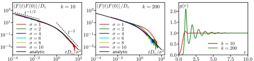
Figure 1: Force autocorrelation for a bath of PBP for varying $\sigma$ for soft interaction $k=10$ (left) and harder interaction $k=200$ (center). Simulations in 2d are compared to the analytic solution Eq. (20). Right: Pair correlation in the fluid showing the increase of the correlation length when $k$ increases. $\rho_{0}=1$, $T=1$, time step $dt=0.003$ and system size $100\times 100$.

Let us first compute the force autocorrelation $\langle\mathbf{F}(t)\cdot\mathbf{F}(0)\rangle_{B}$ for non-interacting bath particles. The element of force $\mathbf{d}F$ exerted on a surface element $dS$ of the tracer around point $\mathbf{r}$ (with the origin at the center of the tracer) is given by the ideal gas law $\mathbf{dF}(0)=-T\rho_{B}(\mathbf{r})dS\frac{\mathbf{r}}{|\mathbf{r}|}$ with $\rho_{B}$ the density of bath particles around a fixed tracer. All particles being independent, contributions to the force autocorrelation come about only due to the same particle returning multiple times to the surface. Denoting the transition probability for a single particle in the presence of a tracer of size $\sigma$ as $P_{\sigma}(\mathbf{r}^{\prime},t|\mathbf{r},0)$, the element of force exerted at time $t$ on surface $dS^{\prime}$ around $\mathbf{r}^{\prime}$ is again given by the ideal gas law $\mathbf{dF}(t)=-TP_{\sigma}(\mathbf{r}^{\prime},t|\mathbf{r},0)dS^{\prime}\frac{\mathbf{r}^{\prime}}{|\mathbf{r}^{\prime}|}$. Integrating over the surface $\mathcal{S}_{T}$ of the tracer reads

$$\langle\mathbf{F}(t)\cdot\mathbf{F}(0)\rangle_{B}=\int_{\mathcal{S}_{T}}dS^{\prime}\int_{\mathcal{S}_{T}}dS\ T^{2}\frac{\mathbf{r}\cdot\mathbf{r}^{\prime}}{|\mathbf{r}||\mathbf{r}^{\prime}|}P_{\sigma}(\mathbf{r}^{\prime},t|\mathbf{r},0)\rho_{B}(\mathbf{r}).$$ (16)

Using the spherical symmetry, we can reduce Eq. (16) to a particle starting on the $x$-axis at $\mathbf{r}=\sigma\mathbf{e}_{x}$ and write, using that anywhere outside the tracer $\rho_{B}(\mathbf{r})=\rho_{0}$, the average density,

$$\langle\mathbf{F}(t)\cdot\mathbf{F}(0)\rangle_{B}=S_{d-1}\sigma^{d-1}\rho_{0}T^{2}\int_{\mathcal{S}_{T}}dS^{\prime}\cos\theta P_{\sigma}(\mathbf{r}^{\prime},t|\sigma\mathbf{e}_{x},0).$$ (17)

where $\theta$ is the angle between $\mathbf{r}$ and the $x$-axis and $S_{d}$ is the solid angle of a $d$-dimensional sphere so that the area of the tracer is $S_{d-1}\sigma^{d-1}$. Finally, we rescale the length by $\sigma$ in the integral, and recognize that $P_{\sigma}(\mathbf{r}^{\prime}/\sigma,t|\mathbf{e}_{x},0)$ can be replaced by the solution of the diffusion equation around a unit tracer with unit diffusion coefficient, but with diffusively rescaled time $(1/\sigma^{d})P_{1}(\mathbf{r},tD_{B}/\sigma|\mathbf{e}_{x},0)$:

$$\langle\mathbf{F}(t)\cdot\mathbf{F}(0)\rangle_{B}=S_{d-1}\sigma^{d-2}\rho_{0}T^{2}\int_{\mathcal{S}_{d-1}}dS^{\prime}\cos\theta P_{1}\left(\mathbf{r}^{\prime},\frac{tD_{B}}{\sigma^{2}}|\mathbf{e}_{x},0\right).$$ (18)

The integral on the r.h.s. of Eq. (18) now runs over the solid angle of a sphere $\mathcal{S}_{d-1}$ and is a dimensionless function of the dimensionless time $\tilde{t}=tD_{B}/\sigma^{2}$ so that we can write

$$\langle\mathbf{F}(t)\cdot\mathbf{F}(0)\rangle_{B}=S_{d-1}\sigma^{d-2}\rho_{0}T^{2}g(tD_{B}/\sigma^{2});\qquad g(\tilde{t})\equiv\int_{\mathcal{S}_{d-1}}dS^{\prime}\cos\theta P_{1}(\mathbf{r}^{\prime},\tilde{t}|\mathbf{e}_{x},0)$$ (19)

The function $g$ can be obtained by solving the diffusion equation around the unit sphere. An explicit expression in terms of Bessel functions is obtained for $d=2$ in B. From Fig. 1, we see that is displays a power-law behavior $g(\tilde{t})\sim\tilde{t}^{-1/2}$ at short times crossing over at $\tilde{t}\approx 1$ to $g(\tilde{t})\sim\tilde{t}^{-2}$.

If the tracer is large enough, the previous calculation also applies straightforwardly to interacting particles, once we recognize that the only hydrodynamic mode in the bath is the density of particles [42]. Indeed, on scales longer than the bath’s correlation length and time, the bath’s particle density follows the diffusion equation $\partial_{t}\rho_{B}=D_{c}\nabla^{2}\rho_{B}$ with a collective diffusion coefficient $D_{c}$. On this scale, this is a full description of the system, which is thus equivalent to non-interacting particles with a diffusion coefficient $D_{c}$. One can then repeat the previous derivation, using that the mechanical pressure on the tracer is now $\Pi=D_{c}\rho_{0}/\mu_{B}$ and obtain

$$\langle\mathbf{F}(t)\cdot\mathbf{F}(0)\rangle_{B}=S_{d-1}\sigma^{d-2}\rho_{0}T\frac{D_{c}}{\mu_{B}}g\left(\frac{D_{c}t}{\sigma^{2}}\right).$$ (20)

Compared to Eq. (19), note that only one of the prefactor $T$ was converted in $D_{c}/\mu_{B}$ in Eq. (20). Indeed, following the reasoning that lead to Eq. (19), the initial element of force $\mathbf{d}\mathbf{F}(0)$ is proportional to $D_{c}/\mu_{B}$ but the one at time $t$, which corresponds to a single particle returning to the tracer, exerts a pressure proportional to $T$.

Let us now compare the predictions of Eq. (20) with results from numerical simulations in 2d. We first look at the effect of the tracer size $\sigma$ in Fig. 1 by showing the measured force autocorrelation rescaled as in Eq. (20) and comparing with the analytic expression obtained for a non-interacting bath. For soft interaction $k=10$ (left panel), the agreement is excellent. For harder interactions $k=200$ (center panel), one observes a deviation for small tracers. This is hardly surprising since, as shown in Fig. 1 (right), pair correlations in the bath extend over a larger distance as $k$ increases. For $k=200$, we see that correlations extend over $\approx 3$ particle radii, consistent with the deviations from scaling, which is expected only when the tracer is larger than the correlation length of the bath.

In Fig. 2 we vary $k$ at a fixed tracer size $\sigma=6$, larger than the correlation length for the range of $k$ values tested. We observe an excellent agreement in the whole range. The collective diffusion coefficient $D_{c}$ used to rescale the curves both in Fig. 1 and Fig. 2 is computed independently in relaxation experiments: Starting with an inhomogeneous initial condition (in our case a stripe), the Fourier mode $\mathbf{q}$ of the density field decays as $\hat{\rho}_{B}(\mathbf{q},t)\propto e^{-D_{c}q^{2}t}$ which allows us to extract $D_{c}$ from the rate of exponential decay. The resulting values of $D_{c}$ are plotted in Fig. 2 (right). Note that the collective diffusion coefficient increases by a factor of $30$ when varying $k$ from $0$ to $200$ which thus provides a significant test of Eq. (20). For larger $k$ values, the correlation length diverges rapidly and our theory does not apply anymore.

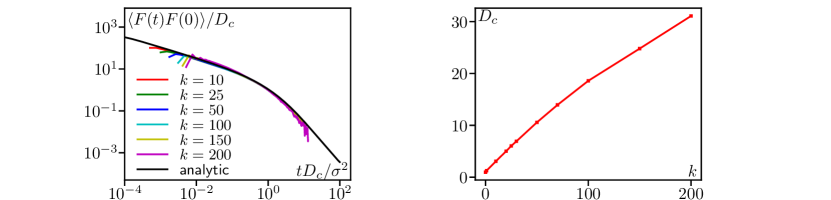
Figure 2: Left: Force autocorrelation for a bath of PBP at fixed $\sigma=6$ for varying interaction strength $k$ showing a good collapse using the collective diffusion $D_{c}$. Parameters: $\rho_{0}=1$, $T=1$, $dt=0.003$ and system size $L=100$. Right: $D_{c}(k)$ measured in relaxation experiments: We start from an inhomogeneous striped initial condition $\rho_{B}(x)=(1-\alpha)\rho_{0}$ if $x<L/2$ and $\rho_{B}(x)=(1+\alpha)\rho_{0}$ if $x>L/2$ with $\alpha=0.1$ and extract $D_{c}$ from the decay of the first Fourier mode $\mathbf{q}=(2\pi/L,0)$, such that $\hat{\rho}_{B}(\mathbf{q},t)\propto e^{-q^{2}D_{c}t}$. Parameters: $L=100$, $dt=10^{-3}$, $\rho_{0}=1$.

3.2 Non-interacting active bath

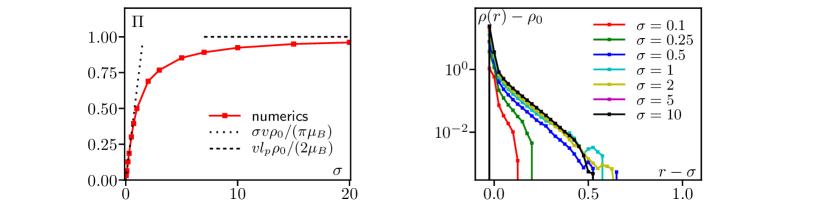
Figure 3: Left: Pressure on the tracer due to a bath of non-interacting ABPs as a function of tracer size $\sigma$ from which the active temperature $T_{a}=\Pi/\rho_{0}$ is defined. The dashed and dotted line indicate the two asymptotic regimes considered in the text. Parameters: $v=2$, $l_{r}=1$, $\rho_{0}=1$. $dt=3\times 10^{-4}$ and $L=10$ for $\sigma<1$. $dt=3\times 10^{-3}$ and $L=60$ for $\sigma>1$. Right: Density profile near the tracer for varying tracer size showing an exponential decay over a small distance. Parameters: $\rho_{0}=1$, $v=2$, $l_{p}=1$, $L=100$, $dt=3\times 10^{-3}$.

Contrary to the passive case, one cannot resort to the Boltzmann distribution to relate $\gamma_{p}$ and the force autocorrelation for active particles. To proceed, let us consider non-interacting particles for which the correlator in $\gamma_{p}$ can be written as an integral over the configuration of a single particle (position $\mathbf{r}$ and orientation $\mathbf{u}$) instead of a full microscopic configuration of the bath. This reads

$$\langle\mathbf{F}(t)\cdot\nabla\log\pi_{B}(0)\rangle_{B}=\int d\mathbf{r}\int d\mathbf{u}\int d\mathbf{r}^{\prime}\int d\mathbf{u}^{\prime}\left[\mathbf{F}(\mathbf{r}^{\prime},\mathbf{u}^{\prime})\cdot\nabla\pi_{B}(\mathbf{r},\mathbf{u})P^{A}_{\sigma}(\mathbf{r}^{\prime},\mathbf{u}^{\prime},t|\mathbf{r},\mathbf{u},0)\right]$$ (21)

where the spatial integrations run over all space and the orientation ones over the unit sphere and $\mathbf{F}(\mathbf{r}^{\prime},\mathbf{u}^{\prime})$ is the force exerted on the tracer by a particle at position $\mathbf{r}^{\prime}$ with orientation $\mathbf{u}^{\prime}$. We have added a superscript $A$ to the conditional probability $P^{A}_{\sigma}$ to distinguish it from the passive case of Sec. 3.1. To make progress, we can use that, for a hard tracer, $\nabla\pi_{B}$ is non-zero only close to the surface where the probability distribution $\pi_{B}(\mathbf{r},\mathbf{u})$ goes rapidly from $0$ inside the tracer to its bulk value $\rho_{0}/S_{d-1}$ (in the bulk all directions are equiprobable). Although hard to prove rigorously, it is clear numerically, as shown in Fig. 3 where the density $\rho_{B}=\int d\mathbf{u}\pi_{B}$ reaches $\rho_{0}$ exponentially on a scale smaller than $\sigma$. On the contrary, $P^{A}_{\sigma}$ varies smoothly over this range so that we can restrict the integration $\int d\mathbf{r}$ to the surface of the tracer. The integration $\int d\mathbf{r}^{\prime}$ is also restricted to the surface since $\mathbf{F}(\mathbf{r}^{\prime},\mathbf{u}^{\prime})$ vanishes elsewhere. Eq. (21) thus simplifies to

$$\langle\mathbf{F}(t)\cdot\nabla\log\pi_{B}(0)\rangle_{B}\approx\int_{\mathcal{S}_{T}}dS\int d\mathbf{u}\int_{\mathcal{S}_{T}}dS^{\prime}\int d\mathbf{u}^{\prime}\left[\mathbf{F}(\mathbf{r}^{\prime},\mathbf{u}^{\prime})\cdot\left(\frac{\rho_{0}}{S_{d-1}}\frac{\mathbf{r}}{|\mathbf{r}|}\right)P^{A}_{\sigma}(\mathbf{r}^{\prime},\mathbf{u}^{\prime},t|\mathbf{r},\mathbf{u},0)\right]$$ (22)

We can now use the ideal gas law to relate Eq. (22) to the force autocorrelation. The mechanical pressure due to non-interacting active particles is a well-defined, measurable, quantity [43]. Let us then introduce the “active temperature” $T_{a}$ such that the pressure on the tracer is $\Pi=T_{a}\rho_{0}$. As in Sec. 3.1, the term $-T_{a}\rho_{0}\frac{\mathbf{r}}{|\mathbf{r}|}$ is then the element of force at time $t=0$ so that Eq. (22) reduces to the force autocorrelation up to a factor $1/T_{a}$, i.e.

$$\langle\mathbf{F}(t)\cdot\nabla\log\pi_{B}(0)\rangle_{B}\approx\frac{1}{T_{a}}\langle\mathbf{F}(t)\cdot\mathbf{F}(0)\rangle_{B}$$ (23)

This implies that $D_{p}=T_{a}\gamma_{p}$ and both can be determined from the force autocorrelation.

Note that the approximation sign in Eq. (23) comes from the fact that $\nabla\pi_{B}(\mathbf{r},\mathbf{u})\neq 0$ over a finite range near the surface of the tracer. For a passive fluid the dependence in $\mathbf{u}$ disappears and $\nabla\pi_{B}(\mathbf{r})=0$ strictly everywhere except at the surface of the tracer so that Eq. (23) becomes an equality in the passive case. The temperature entering the fluctuation-dissipation relation $D_{p}=T\gamma_{p}$ can thus be seen as coming from the ideal gas law.

In addition to replacing $T$ by $T_{a}$, another important difference with the passive case is that the conditional probability $P^{A}_{\sigma}(\mathbf{r}^{\prime},\mathbf{u}^{\prime},t|\mathbf{r},\mathbf{u},0)$ appearing in the correlators needs to be computed for an ABP instead of a PBP. In general, this is not possible analytically and in the following we look separately at the limits when the tracer is either very large or very small compared to the persistence length of the ABPs.

3.2.1 Large tracer

On time scales larger than the persistence time $\tau_{p}=D_{r}^{-1}$, an ABP looses its orientation and is thus effectively diffusing. For large tracers $\sigma\gg l_{p}$, with $l_{p}=v\tau_{p}$ the persistence length, the ABP is thus diffusive before it can leave ballistically the tracer (which happens in a time $\sim\sigma/v$). In this case, the motion approaches that of a passive particles and thus $P^{A}_{\sigma}=P_{\sigma}$ (the dependence on $\mathbf{u}^{\prime}$ and $\mathbf{u}$ in $P^{A}_{\sigma}$ simply becomes irrelevant and can be integrated out). Moreover, as shown in Fig. 3, the pressure on the tracer approaches that on a flat wall [43], giving $T_{a}=\frac{v^{2}}{2D_{r}\mu_{B}}$. The force autocorrelation is then the same as in the passive case Eq. (18) upon replacing $T$ by $T_{a}$ so that

$$\langle\mathbf{F}(t)\cdot\mathbf{F}(0)\rangle_{B}=S_{d-1}\sigma^{d-2}\rho_{0}T_{a}^{2}g\left(\frac{tD_{B}}{\sigma^{2}}\right).$$ (24)

where $D_{B}\equiv\mu_{B}T_{a}$ is the bare diffusion coefficient of an ABP.

Fig. 4 (left) verifies Eq. (24) numerically in $d=2$. One observes that indeed, upon increasing $\sigma$, the autocorrelation approaches the same analytical solution as in Sec. 3.1 for a passive bath. The discrepancy at small $t$ is the signature of the finite persistence of the active particles. However, as $\sigma$ increases, the finite persistence becomes negligible in units of diffusive time $\sigma^{2}/D_{B}$.

3.2.2 Small tracer

In the opposite limit, when $\sigma\ll l_{p}$, an ABP initially in contact with the tracer will move far away before changing its orientation. We then expect the relevant time scale to be the ballistic time to leave the tracer $\sigma/v$. Moreover, in this regime the active temperature $T_{a}$ depends on the tracer size $T_{a}=\frac{v\sigma}{\pi\mu_{B}}$ in $d=2$ as shown numerically in Fig. 3 and Ref. [44]. Consistent with this, the scaling that is observed numerically in Fig. 4 (right) is of the form

$$\langle\mathbf{F}(t)\cdot\mathbf{F}(0)\rangle_{B}=\sigma^{d-2}T_{a}^{2}\rho_{0}h\left(\frac{tv}{\sigma}\right).$$ (25)

and we find numerically in $d=2$ that $h(t)\approx 1.5e^{-t}$. Note that the scalings with $\sigma$, both in time and in amplitude (because $T_{a}$ depends on $\sigma$) are different from the large-tracer case above.

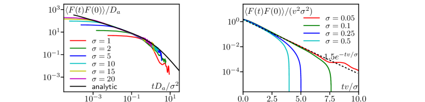
Figure 4: Force autocorrelation for a non-interacting active bath for varying $\sigma$. One observes to regimes with different scaling. For large $\sigma$ (left) the physics is the same as for a passive fluid. The physics at small $\sigma$ (right), on the contrary, comes purely from the activity. Parameters: $v=2$, $l_{r}=1$. $L=150$ and $dt=3\times 10^{-3}$ (left). $L=15$ and $dt=4\times 10^{-4}$ (right).

4 Mobility and diffusivity of the tracer

The coefficients $D_{p}$ and $\gamma_{p}$ appearing in the effective dynamics of the tracer Eq. (9) are obtained by time-integrating the force autocorrelation. For the three cases considered in Sec. 3, integrating Eq. (20), Eq. (24) and Eq. (25) yield respectively

$$D_{p}=c\frac{\sigma^{d}T\rho_{0}}{\mu_{B}}=T\gamma_{p}\quad\, {\rm(passive)}$$ (26)

$$D_{p}=c\frac{\sigma^{d}T_{a}\rho_{0}}{\mu_{B}}=T_{a}\gamma_{p}\quad\, {\rm(active)}\,\sigma\gg l_{p}$$ (27)

$$D_{p}=c^{\prime}\frac{\sigma^{d}T_{a}\rho_{0}}{\mu_{B}}=T_{a}\gamma_{p}\quad\, {\rm(active)}\,\sigma\ll l_{p}$$ (28)

with the constants $c=\frac{S_{d-1}}{d}\int_{0}^{\infty}g(t)dt$ and $c^{\prime}=\frac{\pi}{d}\int_{0}^{\infty}h(t)dt$. The three expressions above are strikingly similar. The differences between these systems are contained in the temperature $T$ or $T_{a}$ (which can depend on $\sigma$) and the geometric constant $c$ or $c^{\prime}$. In the passive case, the collective diffusion coefficient $D_{c}$ that appears in the force autocorrelation drops out at the integration. The dynamics of the tracer is thus blind to the interactions in the bath.

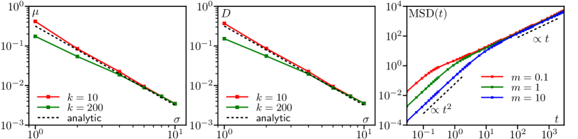
Figure 5: Interacting passive bath. Left: Mobility of the tracer measured as the response to a pulling force small enough (here $f=0.03\sigma^{2}$) to be in the linear regime. Center: Diffusion coefficient measured by fitting the mean-squared displacement of the tracer at late times. Right: Mean-squared displacement as a function of mass for three different values of the mass for $k=10$, $\sigma=1$. Parameters: $m=10$ (except on the right), $L=100$, $dt=3\times 10^{-3}$.

From there, we can compute the diffusivity and mobility of the tracer from Sec. 2 which gives

$$\mu=\frac{1}{\gamma_{T}+\gamma_{p}};\qquad D=\frac{D_{T}+D_{p}}{(\gamma_{T}+\gamma_{p})^{2}}.$$ (29)

Let us first consider the case $\gamma_{T}=0$, meaning that the surrounding fluid does not affect the tracer. This is probably not the most common situation but provides a good test for the effect of the bath on both $\mu$ and $D$. We show results with $\gamma_{T}\neq 0$ at the end of this section. For the passive bath or the active bath with $\sigma\gg l_{p}$, the predictions from Eq. (26) and Eq. (27) are the same

$$\mu=\frac{\mu_{B}}{c\rho_{0}\sigma^{d}};\quad D=\frac{D_{B}}{c\rho_{0}\sigma^{d}}.$$ (30)

In $d=2$ we obtain $c=\pi$ (see B). The active case with small tracers $\sigma\ll l_{p}$ gives

$$\mu=\frac{\mu_{B}}{c^{\prime}\rho_{0}\sigma^{d}};\quad D=\frac{\mu_{B}T_{a}}{c^{\prime}\rho_{0}\sigma^{d}}.$$ (31)

with $T_{a}=\sigma v/(\pi\mu_{B})$ and $c^{\prime}\approx 1.05$ in $d=2$.

We want to compare our predictions to numerical measurements of $D$ and $\mu$. The mobility is computed from its definition Eq. (11) by applying a constant external force and measuring the average velocity reached by the tracer. We ensured that we are in the linear regimes by repeating the measurement for different values of the external force. The diffusivity is fitted on the late-time mean squared displacement of the tracer, in absence of any external force. In measuring $D$ and $\mu$, we make sure that we have reached the limit where the tracer is heavy, the hypothesis used in the calculation of Sec. 2. In practice, as exemplified in Fig. 5 (right) for the diffusion coefficient, the variation with $m$ is no more than a few percent and we found that using $m=10$ for all parameters is enough to ensure convergence.

The predictions are compared without any fitting parameter to the numerical simulations in Fig. 5 for the passive bath and Fig. 6 for the active one. For the passive bath, the agreement is prefect within numerical accuracy except for the expected deviation for tracers smaller than the correlation length of the bath. In the active case of Fig. 6 the agreement is again perfect when the tracer becomes large. At small $\sigma$, we find a systematic discrepancy of about $25\%$ in the non-interacting case, which can be explained by the approximation made in Sec. 3.2. Nonetheless, the theory captures the correct order of magnitude and, for $D$, the correct change in behavior with $D\propto\sigma^{-1}$ at small $\sigma$ and $D\propto\sigma^{-2}$ at large $\sigma$.

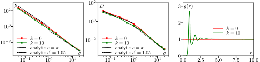
Figure 6: Non-interacting and interacting active baths. Mobility (left) and diffusion coefficient (center) measured as in Fig. 5. Parameters: $m=10$ and either $L=150$, $dt=3\times 10^{-3}$ for $\sigma<1$ or $L=15$, $dt=3\times 10^{-4}$ for $\sigma\geq 1$. Right: Pair correlation in the bath showing that $k=10$ corresponds to a much higher interaction level than in the passive case (see text).

If the active particles in the bath are interacting, we expect the physics to be more complex since there are three length scales in the system: the tracer size $\sigma$, the bath particle size and the persistence length. However, in the limit of large $\sigma$, we expect the same argument leading to Eq. (20) in the passive case to be applicable. Consistently, we observe numerically in Fig. 6 that the values of $D$ and $\mu$ do not depend on the interaction strength $k$ for large $\sigma$. For smaller $\sigma$, their values depend slightly on $k$ but the asymptotic scalings $\mu\propto\sigma^{-2}$ and $D\propto\sigma^{-1}$ are not modified. Note that the value of the interaction strength $k=10$ corresponds in the active case to a rather strong interaction with several peaks in the pair correlation function, as shown in Fig. 6 (right) while it was close to the non-interacting limit in the passive case of Fig. 1. This difference is not surprising. Indeed, for the ballistic motion of ABPs the overlap $\delta$ between two particles is of order $\delta\approx v/(\mu_{B}k)$ while for the diffusive PBPs $\delta\approx\sqrt{T/k}$ so that the active particles become effectively stiffer more rapidly than passive ones as $k$ increases.

Let us finally consider the case when the external fluid acts on the tracer with a coefficient $\gamma_{T}\neq 0$. This is the most relevant case experimentally since the most common active particles such as bacteria or self-propelled colloids move in a fluid. The mobility and diffusivity of the tracer is then given by Eq. (29). To verify numerically this formula, we used the values of $\gamma_{p}$ and $D_{p}$ measured when $\gamma_{T}=0$ and extrapolate to $\gamma_{T}\neq 0$ using Eq. (29). We see in Fig. 7 that the agreement with direct measurements is perfect up to numerical accuracy.

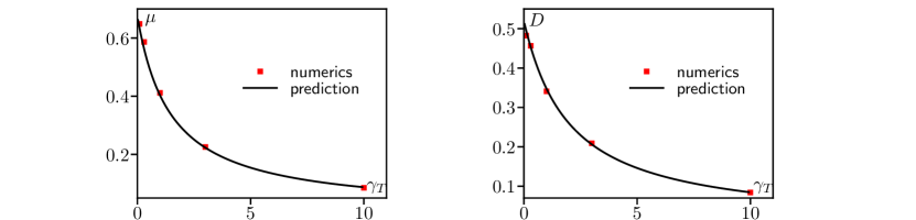
Figure 7: Effect of the external fluid friction with coefficient $\gamma_{T}$ on the mobility (left) and diffusivity (right) for an non-interacting active bath and a tracer size $\sigma=1$. On both panels, the prediction curve is that of Eq. (29), using the $\gamma_{p}$ and $D_{p}$ measured at $\gamma_{T}=0$. Parameters: $k=0$, $m=10$, $L=150$, $dt=3\times 10^{-3}$.

5 Discussion

In deriving the Einstein relation, our approach based on the effective dynamics of the tracer makes clear that the temperature $T$ appearing in the Einstein relation for a passive bath comes in through the ideal gas law when computing the force autocorrelation in Sec. 3. Although an active bath is not characterized by a single temperature, the mechanical pressure is a perfectly well-defined quantity [43]. This leads us naturally to define an “active temperature” $T_{a}$ as the quantity appearing in the ideal gas law and therefore appearing also in the fluctuation-dissipation relation $D_{p}=T_{a}\gamma_{p}$ albeit this is only an approximation in the active case.

When the tracer is subject to both thermal noise and the active bath, the temperatures associated to the two processes do not simply add. Instead the coefficient in the $T_{\rm eff}$ such that $D=\mu T_{\rm eff}$ reads from Eq. (13)

$$T_{\rm eff}=\frac{T\gamma_{T}+T_{a}\gamma_{p}}{\gamma_{T}+\gamma_{p}}$$ (32)

which features the damping coefficients due to the fluid and to the bath, respectively $\gamma_{T}$ and $\gamma_{p}$. Different regimes are then obtained depending on the parameters. When $\gamma_{T}\to 0$, as in Fig. 6, the fluid does not affect the tracer so that $T_{\rm eff}=T_{a}$. When $\gamma_{T}\gg\gamma_{p}$ but $T_{a}\gamma_{p}\gg T\gamma_{T}$, the damping is controlled by the fluid but the diffusivity comes from the active bath. As discussed in the introduction, this is the regime in which most experiments are performed. One then has $T_{\rm eff}=T_{a}\gamma_{p}/\gamma_{T}$. Ultimately, when $\gamma_{T}\gg\gamma_{p}$ and $T\gamma_{T}\gg T_{a}\gamma_{p}$, we reach a passive limit with $T_{\rm eff}=T$.

Finally, let us remark that for large tracers the values of $D$ and $\mu$ appear universal for both passive and active baths. In this limit we obtained

$$\mu=\frac{\mu_{B}}{c\rho_{0}\sigma^{d}};\quad D=\frac{D_{B}}{c\rho_{0}\sigma^{d}};$$ (33)

where the only effect of the bath is through the bare (i.e. single particle) mobility and diffusion coefficient $\mu_{B}$ and $D_{B}$. This is in stark contrast to simple equilibrium fluids, where the Stokes-Einstein relation connects the diffusivity of a large, heavy tracer to the bath’s viscosity $D\propto 1/\eta$ (in 3D). While there is no viscosity for Brownian baths as momentum is not conserved and therefore not relevant on hydrodynamic scales, one still might suspect that collective properties of the bath affect a tracer’s dynamics. However, we have observed that large tracers are blind to the collective transport properties of the bath, which can be accessed only using tracers that are smaller than the correlation length of a passive bath or the persistence length of an active one. We believe that our understanding of this issue would benefit from a mode-coupling analysis like that carried out in Ref. [45] to derive the Stokes-Einstein relation from the microscopic Hamiltonian dynamics, where it was shown that one must actually include all higher-order modes to correctly extract the Stokes-Einstein relation.

Note that in this article we have considered only pairwise interaction between bath particles. For active particles, other types of interaction such as quorum-sensing or nonreciprocal ones are possible and more complex phenomena such as flocking and motility-induced phase separation could happen in the bath. The dynamics of a tracer in these complex fluids is an open problem.

Appendix A Derivation of the effective tracer dynamics using projection operators

In this Appendix, we review the projection operator technique for extracting the reduced equations for the tracer particle. The methodology is standard [29, 30, 39], with our derivation following closely the original exposition for equilibrium fluids [40].

The probability distribution for the joint position of the tracer in its phase space $({\mathbf{R}},{\mathbf{P}})$ and the positions of the overdamped Brownian bath particles $\{{\bf r}_{i}\}$ evolves according the Fokker-Planck equation [29]

$$\partial_{t}P({\mathbf{R}},{\mathbf{P}},{\mathbf{r}}_{i})={\mathcal{L}}_{T}P({\mathbf{R}},{\mathbf{P}},{\mathbf{r}}_{i})+{\mathcal{L}}_{B}P({\mathbf{R}},{\mathbf{P}},{\mathbf{r}}_{i}),$$ (34)

where the tracer dynamics are generated by the Fokker-Planck operator

$${\mathcal{L}}_{T}=-\frac{1}{m}\nabla_{\mathbf{R}}\cdot{\mathbf{P}}-\nabla_{\mathbf{P}}\left({\mathbf{F}}-\frac{\gamma_{T}}{m}\mathbf{P}\right)+D_{T}\nabla_{\mathbf{P}}^{2}$$ (35)

and the bath dynamics are generated by one of two operators depending on whether they are passive (PBP) or active (ABP)

$${\mathcal{L}}_{B}=\left\{\begin{array}[]{ll}-\mu_{B}\sum_{i}\nabla_{{\mathbf{r}}_{i}}\cdot\left({\mathbf{f}}_{i}-{\mathbf{F}}_{i}\right)+D_{B}\nabla_{{\mathbf{r}}_{i}}^{2}&{\rm(PBP)}\\ -\mu_{B}\sum_{i}\nabla_{{\mathbf{r}}_{i}}\cdot\left({\mathbf{f}}_{i}-{\mathbf{F}}_{i}\right)-v_{0}\nabla_{{\mathbf{r}}_{i}}\cdot{\mathbf{u}}_{i}+D_{r}\partial_{\theta_{i}}^{2}&{\rm(ABP)}\end{array}\right..$$ (36)

Within the projector-operator formalism we assume that the bath relaxation time is fast compared to the tracer relaxation time. Thus, we expect that with the tracer fixed, the bath will quickly relax to its steady state distribution conditioned on the position of the tracer $\pi_{B}({\mathbf{r}}_{i}|{\mathbf{R}})$ given as the solution of

$${\mathcal{L}}_{B}\pi_{B}({\mathbf{r}}_{i}|{\mathbf{R}})=0.$$ (37)

We will assume that this distribution is unique, or, put another way, the null space of ${\mathcal{L}}_{B}$ is one dimensional. We will also find it convenient to introduce a notation for steady-state averages with the tracer fixed as $\langle A\rangle_{B}=\int\prod_{i}d{\mathbf{r}}_{i}A({\mathbf{r}}_{i})\pi_{B}({\mathbf{r}}_{i}|{\mathbf{R}})$.

To exploit this separation of time-scales we introduce a projection operator that projects the bath distribution onto the fixed-tracer steady-state distribution

$${\mathcal{P}}P({\mathbf{R}},{\mathbf{P}},{\mathbf{r}}_{i})=\pi_{B}({\mathbf{r}}_{i}|{\mathbf{R}})\int\prod_{i}d{\mathbf{r}}_{i}P({\mathbf{R}},{\mathbf{P}},{\mathbf{r}}_{i})\equiv\pi_{B}({\mathbf{r}}_{i}|{\mathbf{R}})\rho({\mathbf{R}},{\mathbf{P}}),$$ (38)

as well as the orthogonal projector ${\mathcal{Q}}={\mathcal{I}}-{\mathcal{P}}$, where ${\mathcal{I}}$ is the identity operator. Note, that as is required for a useful projection operator, it projects away the bath dynamics

$${\mathcal{L}}_{B}{\mathcal{P}}={\mathcal{P}}{\mathcal{L}}_{B}=0,$$ (39)

which can be verified from the definitions of the operators.

We next apply ${\mathcal{P}}$ and ${\mathcal{Q}}$ to (34) from the left, and insert the identity operator ${\mathcal{I}}={\mathcal{P}}+{\mathcal{Q}}$ to the right of the Fokker-Planck operators to obtain the pair of equations for the relevant part ${\mathcal{P}}P$ and irrelevant part ${\mathcal{Q}}P$,

$$\partial_{t}{\mathcal{P}}P={\mathcal{P}}{\mathcal{L}}_{T}{\mathcal{P}}P+{\mathcal{P}}{\mathcal{L}}_{T}{\mathcal{Q}}P$$ (40)

$$\partial_{t}{\mathcal{Q}}P={\mathcal{Q}}{\mathcal{L}}_{B}{\mathcal{Q}}P+{\mathcal{Q}}{\mathcal{L}}_{T}{\mathcal{P}}P+{\mathcal{Q}}{\mathcal{L}}_{T}{\mathcal{Q}}P,$$ (41)

where we have suppressed the arguments of the probability distribution to avoid cluttering the equations. Typically at this point one solves the equation for the irrelevant part ${\mathcal{Q}}P$ formally and substitutes it back into the equation for the relevant part ${\mathcal{P}}P$ [30]. To obtain a manageable equation, one then typically makes the uncontrolled Markov approximation. Here, we will take a slightly more circuitous route that gives the same results, but has the advantage of making the approximations more clear.

To this end, let us formally introduce a small parameter $\epsilon\ll 1$ into the equation for the irrelevant part ${\mathcal{Q}}P$ to make explicit the time-scale separation between fast bath and slow tracer dynamics:

$$\partial_{t}{\mathcal{Q}}P=\frac{1}{\epsilon}{\mathcal{Q}}{\mathcal{L}}_{B}{\mathcal{Q}}P+{\mathcal{Q}}{\mathcal{L}}_{T}{\mathcal{P}}P+{\mathcal{Q}}{\mathcal{L}}_{T}{\mathcal{Q}}P.$$ (42)

At the end, we will set $\epsilon=1$. We can now look for a perturbative solution of the form

$${\mathcal{Q}}P=q^{(0)}+\epsilon q^{(1)}+\cdots.$$ (43)

Substituting this into (42), we can now solve order by order in $\epsilon$. At lowest order we find

$${\mathcal{Q}}{\mathcal{L}}_{B}q^{(0)}=(1-{\mathcal{P}}){\mathcal{L}}_{B}q^{(0)}={\mathcal{L}}_{B}q^{(0)}=0,$$ (44)

upon using (39). This equation implies that $q^{(0)}$ is in the null space of ${\mathcal{L}}_{B}$. However, by definition ${\mathcal{Q}}P$ is orthogonal to the null space of ${\mathcal{L}}_{B}$. Thus, the only solution is $q^{(0)}=0$. At the next order we have

$${\mathcal{Q}}{\mathcal{L}}_{B}q^{(1)}+{\mathcal{Q}}{\mathcal{L}}_{T}{\mathcal{P}}P=0.$$ (45)

We can solve this formally, to get the first nontrivial solution for the irrelevant part

$${\mathcal{Q}}P\approx q^{(1)}={\mathcal{Q}}\int_{0}^{\infty}ds\ e^{{\mathcal{L}}_{B}s}{\mathcal{Q}}{\mathcal{L}}_{T}{\mathcal{P}}P,$$ (46)

now setting $\epsilon=1$ as it is no longer needed.

Having approximated the irrelevant part of the dynamics, we can derive a closed equation for the relevant dynamics by substituting (46) into (40),

$$\partial_{t}{\mathcal{P}}P={\mathcal{P}}{\mathcal{L}}_{T}{\mathcal{P}}P+{\mathcal{P}}{\mathcal{L}}_{T}{\mathcal{Q}}\int_{0}^{\infty}ds\ e^{{\mathcal{L}}_{B}s}{\mathcal{Q}}{\mathcal{L}}_{T}{\mathcal{P}}P.$$ (47)

We now turn to evaluating each term using the definitions of the operators. The first term represents the Eulerian part of the dynamics:

$${\mathcal{P}}{\mathcal{L}}_{T}{\mathcal{P}}P ={\mathcal{P}}\left[-\frac{1}{m}\nabla_{\mathbf{R}}{\mathbf{P}}-\nabla_{\mathbf{P}}\left({\mathbf{F}}-\frac{\gamma_{T}}{m}\mathbf{P}\right)+D_{T}\nabla_{\mathbf{P}}^{2}\right]\pi_{\rm B}\rho$$ (48)

$$={\mathcal{P}}\pi_{B}\left[-\frac{{\mathbf{P}}}{m}(\nabla_{\mathbf{R}}\ln\pi_{B})-\frac{1}{m}\nabla_{\mathbf{R}}{\mathbf{P}}-\nabla_{\mathbf{P}}\left({\mathbf{F}}-\frac{\gamma_{T}}{m}\mathbf{P}\right)+D_{T}\nabla_{\mathbf{P}}^{2}\right]\rho$$ (49)

$$=\pi_{B}\left[-\frac{{\mathbf{P}}}{m}\langle\nabla_{\mathbf{R}}\ln\pi_{B}\rangle_{B}-\frac{1}{m}\nabla_{\mathbf{R}}{\mathbf{P}}-\nabla_{\mathbf{P}}\left(\langle{\mathbf{F}}\rangle_{B}-\frac{\gamma_{T}}{m}\mathbf{P}\right)+D_{T}\nabla_{\mathbf{P}}^{2}\right]\rho$$ (50)

$$=\pi_{B}\left[-\frac{1}{m}\nabla_{\mathbf{R}}{\mathbf{P}}+\frac{\gamma_{T}}{m}\nabla_{\mathbf{P}}\mathbf{P}+D_{T}\nabla_{\mathbf{P}}^{2}\right]\rho,$$ (51)

where in the last line we used the assumed spherical symmetry of the tracer-bath force to set $\langle{\mathbf{F}}\rangle_{B}=0$ and the fact that $\langle\nabla_{\mathbf{R}}\ln\pi_{B}\rangle_{B}=0$, as $\pi_{B}$ is normalized. For the second dissipative term we evaluate the effect of the operators one at a time:

$${\mathcal{P}}{\mathcal{L}}_{T}{\mathcal{Q}}e^{{\mathcal{L}}_{B}s}{\mathcal{Q}}{\mathcal{L}}_{T}{\mathcal{P}}P$$ (52)

$$={\mathcal{P}}{\mathcal{L}}_{T}{\mathcal{Q}}e^{{\mathcal{L}}_{B}s}{\mathcal{Q}}\pi_{B}\left[-\frac{{\mathbf{P}}}{m}\langle\nabla_{\mathbf{R}}\ln\pi_{B}\rangle_{B}-\frac{1}{m}\nabla_{\mathbf{R}}{\mathbf{P}}-\nabla_{\mathbf{P}}\left(\langle{\mathbf{F}}\rangle_{B}-\frac{\gamma_{T}}{m}\mathbf{P}\right)+D_{T}\nabla_{\mathbf{P}}^{2}\right]\rho$$ (53)

$$={\mathcal{P}}{\mathcal{L}}_{T}{\mathcal{Q}}e^{{\mathcal{L}}_{B}s}\pi_{B}\left[-\frac{{\mathbf{P}}}{m}(\nabla_{\mathbf{R}}\ln\pi_{B})-\nabla_{\mathbf{P}}{\mathbf{F}}\right]\rho$$ (54)

$$={\mathcal{P}}{\mathcal{L}}_{T}e^{{\mathcal{L}}_{B}s}\pi_{B}\left[-\frac{{\mathbf{P}}}{m}(\nabla_{\mathbf{R}}\ln\pi_{B})-\nabla_{\mathbf{P}}{\mathbf{F}}\right]\rho$$ (55)

$$={\mathcal{P}}\left[-\frac{1}{m}\nabla_{\mathbf{R}}{\mathbf{P}}-\nabla_{\mathbf{P}}\left({\mathbf{F}}-\frac{\gamma_{T}}{m}\mathbf{P}\right)+D_{T}\nabla_{\mathbf{P}}^{2}\right]e^{{\mathcal{L}}_{B}s}\pi_{B}\left[-\frac{{\mathbf{P}}}{m}(\nabla_{\mathbf{R}}\ln\pi_{B})-\nabla_{\mathbf{P}}{\mathbf{F}}\right]\rho$$ (56)

$$=\pi_{B}\left[\nabla_{\mathbf{P}}\left\langle{\mathbf{F}}e^{{\mathcal{L}}_{B}s}\nabla_{\mathbf{R}}\ln\pi_{B}\right\rangle_{B}\frac{{\mathbf{P}}}{m}+\nabla_{\mathbf{P}}\left\langle{\mathbf{F}}e^{{\mathcal{L}}_{B}s}{\mathbf{F}}\right\rangle_{B}\nabla_{\mathbf{P}}\right]\rho$$ (57)

Thus,

$${\mathcal{P}}{\mathcal{L}}_{T}{\mathcal{Q}}\int_{0}^{\infty}ds\ e^{{\mathcal{L}}_{B}s}{\mathcal{Q}}{\mathcal{L}}_{T}{\mathcal{P}}P=\pi_{B}\left[\nabla_{\mathbf{P}}\cdot\hat{\gamma}_{p}\cdot\frac{{\mathbf{P}}}{m}+\nabla_{\mathbf{P}}\cdot\hat{D}_{p}\cdot\nabla_{\mathbf{P}}\right]\rho,$$ (58)

having identified

$$\hat{\gamma}_{p}=\int_{0}^{\infty}\left\langle{\mathbf{F}}e^{{\mathcal{L}}_{B}s}\nabla_{\mathbf{R}}\ln\pi_{B}\right\rangle_{B}ds=\int_{0}^{\infty}\left\langle{\mathbf{F}}(s)\nabla_{\mathbf{R}}\ln\pi_{B}(0)\right\rangle_{B}ds$$ (59)

$${\hat{D}}_{p}=\int_{0}^{\infty}\left\langle{\mathbf{F}}e^{{\mathcal{L}}_{B}s}{\mathbf{F}}\right\rangle_{B}ds=\int_{0}^{\infty}\left\langle{\mathbf{F}}(s){\mathbf{F}}(0)\right\rangle_{B}ds,$$ (60)

which we recognize as operator representations of steady-state correlation functions. These expressions can be simplified using spherical symmetry to conclude that they are both proportional to the identify $\hat{\gamma}_{p}=\gamma_{p}{\hat{I}}$ and ${\hat{D}}_{p}=D_{p}{\hat{I}}$ and by replacing $\nabla_{\mathbf{R}}\to-\nabla$ due to the translational invariance of the bath steady state, thereby arriving at (10).

Finally, putting everything together, we find a closed equation for the tracer dynamics

$$\partial_{t}\rho=\left[-\frac{1}{m}\nabla_{\mathbf{R}}{\mathbf{P}}+\frac{\gamma_{T}+\gamma_{P}}{m}\nabla_{\mathbf{P}}\cdot\mathbf{P}+(D_{T}+D_{p})\nabla^{2}_{\mathbf{P}}\right]\rho,$$ (61)

where the equivalent Langevin equation is used in (9).

Appendix B Exact force-force correlation for a passive particle in 2D

In this Appendix, we solve the 2D diffusion equation around a disk in order to find an explicit expression for $g(t)$ (19), which captures the time-dependence of the correlation function of the force on the tracer due to a bath of independent passive Brownian particles.

Determining the force correlation function is equivalent to finding the Green’s function for a Brownian particle diffusing in an annulus of inner radius $\sigma$ and outer radius $L$. For large $L$, the shape of the region should be immaterial, allowing us to compare the results of this analytical calculation to the simulations. Denoting the position of the particle as $(r,\theta)$ in polar coordinates, we obtain the Green’s function as the solution of the diffusion equation for the time-dependent probability distribution $P(r,\theta,t)$,

$$\partial_{t}P(r,\theta,t)=\nabla^{2}P(r,\theta,t)=\frac{1}{r}\partial_{r}\left[r\partial_{r}P(r,\theta,t)\right]+\frac{1}{r^{2}}\partial_{\theta}^{2}P(r,\theta,t),$$ (62)

with delta-function initial condition at the point $(r_{0},\theta_{0})$ and no flux boundary conditions,

$$P(r,\theta,0)=\delta(r-r_{0})\delta(\theta-\theta_{0})/r_{0}$$ (63)

$$\partial_{r}P(\sigma,\theta,t)=\partial_{r}P(L,\theta,t)=0,\quad P(r,0,t)=P(r,2\pi,t).$$ (64)

The solution can be obtained using an eigendecomposition

$$P(r,\theta,t)=\sum_{\lambda}e^{-\lambda t}f_{\lambda}(r,\theta)f_{\lambda}(r_{0},\theta_{0}),$$ (65)

where the eigenfunctions $f_{\lambda}$ satisfy

$$-\lambda f(r,\theta)=\frac{1}{r}\partial_{r}\left[r\partial_{r}f(r,\theta)\right]+\frac{1}{r^{2}}\partial_{\theta}^{2}f(r,\theta).$$ (66)

While the solution is well known in general, imposing the no-flux boundary conditions requires some delicate analysis, so we review the solution here.

To proceed we look for separable solutions $f_{\lambda}(r,\theta)=R(r)\Theta(\theta)$. Substituting this ansatz into (66), we find that the pair of functions $R$ and $\Theta$ must satisfy

$$\partial_{\theta}^{2}\Theta(\theta)+l^{2}\Theta(\theta)=0$$ (67)

$$r^{2}\partial_{r}^{2}R(r)+r\partial_{r}R(r)+\left(\lambda r^{2}-l^{2}\right)R(r)^{2}=0,$$ (68)

where the constants $\lambda$ and $l$ are fixed by the boundary conditions. To satisfy the periodic boundary condition, $\Theta(0)=\Theta(2\pi)$, we find that $l=n$ with $n\in{\mathbb{N}}$ and then (67) has two possible solutions

$$\Theta(\theta)=\left\{\begin{array}[]{c}\cos(n\theta)\\ \sin(n\theta)\end{array}\right.,$$ (69)

when $n\neq 0$ and is simply $\Theta(\theta)=1$ when $n=0$.

With $l=n$ an integer, we recognize that (68) is Bessel’s equation, whose solution can be written in terms of $n$-th order Bessel functions of the first $J_{n}$ and second $Y_{n}$ kind,

$$R(r)=AJ_{n}(\sqrt{\lambda}r)+BY_{n}(\sqrt{\lambda}r),$$ (70)

where the constants $A$ and $B$ are fixed by imposing the no-flux boundary conditions ($\partial_{r}R(\sigma)=\partial_{r}R(L)=0$):

$$AJ^{\prime}_{n}(\sqrt{\lambda}\sigma)+BY^{\prime}_{n}(\sqrt{\lambda}\sigma)=0$$ (71)

$$AJ^{\prime}_{n}(\sqrt{\lambda}L)+BY^{\prime}_{n}(\sqrt{\lambda}L)=0.$$ (72)

To have nontrivial solutions for $A$ and $B$ the two equations must be linearly dependent, which will only be true when the determinant vanishes,

$$\qquad\left|\begin{array}[]{cc}J^{\prime}_{n}(\sqrt{\lambda}\sigma)&Y^{\prime}_{n}(\sqrt{\lambda}\sigma)\\ J^{\prime}_{n}(\sqrt{\lambda}L)&Y^{\prime}_{n}(\sqrt{\lambda}L)\end{array}\right|=J^{\prime}_{n}(\sqrt{\lambda}\sigma)Y^{\prime}_{n}(\sqrt{\lambda}L)-J^{\prime}_{n}(\sqrt{\lambda}L)Y^{\prime}_{n}(\sqrt{\lambda}\sigma)=0.$$ (73)

This is the required condition to fix the eigenvalues $\lambda$. To exploit this, let us define the zeros $\alpha_{nm}$ of the determinant equation as

$$J^{\prime}_{n}(\alpha_{nm}\sigma)Y^{\prime}_{n}(\alpha_{nm}L)-J^{\prime}_{n}(\alpha_{nm}L)Y^{\prime}_{n}(\alpha_{nm}\sigma)=0.$$ (74)

Then the eigenvalues are $\lambda=\alpha_{nm}^{2}$, and our solution becomes

$$R(r)=AJ_{n}(\alpha_{nm}r)+BY_{n}(\alpha_{nm}r).$$ (75)

We can now fix one of the constants using either of the boundary conditions (71)-(72), as they are now linearly dependent. The radial component of the eigenfunction is then

$$R_{nm}(r)=J_{n}(\alpha_{nm}r)Y^{\prime}_{n}(\alpha_{nm}L)-Y_{n}(\alpha_{nm}r)J^{\prime}_{n}(\alpha_{nm}L),$$ (76)

as long $n>0$ and $m>0$. However, when $n=0$, then $\lambda=0$ is a possible solution. In this case, $R_{00}(r)=1$.

Putting it all together and normalizing, we find for our eigenfunctions

$$f_{nm}(r,\theta)=\frac{1}{\pi N_{nm}}R_{nm}(r)\times\left\{\begin{array}[]{c}\cos(n\theta)\\ \sin(n\theta)\end{array}\right.\quad n,m\geq 1$$ (79)

$$f_{0m}(r,\theta)=\frac{1}{2\pi N_{0m}}R_{0m}(r), n=0,m\geq 1$$ (80)

$$f_{00}(r,\theta)=\frac{1}{\pi(L^{2}-\sigma^{2})}, n=m=0$$ (81)

where we have introduced the normalization $N_{nm}=\int_{\sigma}^{L}R_{nm}(r)^{2}rdr$. Substituting into (65), we arrive at our final expression for the Green’s function

$$P(r,\theta,t|r_{0},\theta_{0},0) =\frac{1}{\pi(L^{2}-a^{2})}+\frac{1}{2\pi}\sum_{m\geq 1}e^{-\alpha_{0m}^{2}t}\frac{R_{0m}(r)R_{0m}(r_{0})}{N_{0m}}$$ (82)

$$\qquad\qquad+\frac{1}{\pi}\sum_{n,m\geq 1}e^{-\alpha_{nm}^{2}t}\frac{R_{nm}(r)R_{nm}(r_{0})}{N_{nm}}\left(\cos(n\theta)\cos(n\theta_{0})+\sin(n\theta)\sin(n\theta_{0})\right).$$ (83)

With the Green’s function in hand, all that is left is to obtain $g(t)$ is to evaluate the integral in (19) for a tracer of radius $\sigma=1$ in two dimensions,

$$g(t)=\int_{0}^{2\pi}\cos(\theta)P(1,\theta,t|1,0,0)d\theta.$$ (84)

We observe that $\cos(\theta)$ is orthogonal to every eigenfunction except when $n=1$. As a result,

$$g(t)=\sum_{m\geq 1}e^{-\alpha_{1m}^{2}t}\frac{R_{1m}(1)^{2}}{N_{1m}},$$ (85)

Data in figures were generated by numerically approximating this sum using the first 1000 nonzero eigenvalues for parameter values $\sigma=1$ and $L=25$.

References

- [1] Xiao-Lun Wu and Albert Libchaber. Particle diffusion in a quasi-two-dimensional bacterial bath. Physical Review Letters, 84(13):3017, 2000.
- [2] Min Jun Kim and Kenneth S Breuer. Controlled mixing in microfluidic systems using bacterial chemotaxis. Analytical chemistry, 79(3):955–959, 2007. Publisher: ACS Publications.
- [3] Sergey Belan and Mehran Kardar. Pair dispersion in dilute suspension of active swimmers. The Journal of Chemical Physics, 150(6):064907, 2019.
- [4] Daniel TN Chen, AWC Lau, Lawrence A Hough, Mohammad F Islam, Mark Goulian, Thomas C Lubensky, and Arjun G Yodh. Fluctuations and rheology in active bacterial suspensions. Physical Review Letters, 99(14):148302, 2007. Publisher: APS.
- [5] Kyriacos C Leptos, Jeffrey S Guasto, Jerry P Gollub, Adriana I Pesci, and Raymond E Goldstein. Dynamics of enhanced tracer diffusion in suspensions of swimming eukaryotic microorganisms. Physical Review Letters, 103(19):198103, 2009. Publisher: APS.
- [6] Chantal Valeriani, Martin Li, John Novosel, Jochen Arlt, and Davide Marenduzzo. Colloids in a bacterial bath: simulations and experiments. Soft Matter, 7(11):5228–5238, 2011. Publisher: Royal Society of Chemistry.
- [7] Gastón Mino, Thomas E Mallouk, Thierry Darnige, Mauricio Hoyos, Jeremi Dauchet, Jocelyn Dunstan, Rodrigo Soto, Yang Wang, Annie Rousselet, and Eric Clement. Enhanced diffusion due to active swimmers at a solid surface. Physical Review Letters, 106(4):048102, 2011. Publisher: APS.
- [8] Raphaël Jeanneret, Dmitri O Pushkin, Vasily Kantsler, and Marco Polin. Entrainment dominates the interaction of microalgae with micron-sized objects. Nature Communications, 7(1):1–7, 2016. Publisher: Nature Publishing Group.
- [9] Claudio Maggi, Matteo Paoluzzi, Luca Angelani, and Roberto Di Leonardo. Memory-less response and violation of the fluctuation-dissipation theorem in colloids suspended in an active bath. Scientific reports, 7(1):1–7, 2017. Publisher: Nature Publishing Group.
- [10] Levke Ortlieb, Salima Rafaï, Philippe Peyla, Christian Wagner, and Thomas John. Statistics of colloidal suspensions stirred by microswimmers. Physical Review Letters, 122(14):148101, 2019. Publisher: APS.
- [11] Antoine Lagarde, Noémie Dagès, Takahiro Nemoto, Vincent Démery, Denis Bartolo, and Thomas Gibaud. Colloidal transport in bacteria suspensions: from bacteria collision to anomalous and enhanced diffusion. Soft Matter, 16(32):7503–7512, 2020. Publisher: Royal Society of Chemistry.
- [12] Hunter Seyforth, Mauricio Gomez, W Benjamin Rogers, Jennifer L Ross, and Wylie W Ahmed. Non-equilibrium fluctuations and nonlinear response of an active bath. arXiv preprint arXiv:2110.15917, 2021.
- [13] Todd M Squires and John F Brady. A simple paradigm for active and nonlinear microrheology. Physics of Fluids, 17(7):073101, 2005. Publisher: American Institute of Physics.
- [14] Patrick T Underhill, Juan P Hernandez-Ortiz, and Michael D Graham. Diffusion and spatial correlations in suspensions of swimming particles. Physical Review Letters, 100(24):248101, 2008. Publisher: APS.
- [15] Zhi Lin, Jean-Luc Thiffeault, and Stephen Childress. Stirring by squirmers. Journal of Fluid Mechanics, 669:167–177, 2011. Publisher: Cambridge University Press.
- [16] Dmitri O Pushkin and Julia M Yeomans. Fluid mixing by curved trajectories of microswimmers. Physical Review Letters, 111(18):188101, 2013. Publisher: APS.
- [17] Alexander Morozov and Davide Marenduzzo. Enhanced diffusion of tracer particles in dilute bacterial suspensions. Soft Matter, 10(16):2748–2758, 2014. Publisher: Royal Society of Chemistry.
- [18] Jean-Luc Thiffeault. Distribution of particle displacements due to swimming microorganisms. Physical Review E, 92(2):023023, 2015. Publisher: APS.
- [19] Charles Reichhardt and CJ Olson Reichhardt. Active microrheology in active matter systems: Mobility, intermittency, and avalanches. Physical Review E, 91(3):032313, 2015.
- [20] Eric W Burkholder and John F Brady. Tracer diffusion in active suspensions. Physical Review E, 95(5):052605, 2017. Publisher: APS.
- [21] Sara Dal Cengio, Demian Levis, and Ignacio Pagonabarraga. Linear response theory and Green-Kubo relations for active matter. Physical review letters, 123(23):238003, 2019.
- [22] Miloš Knežević, Luisa E Avilés Podgurski, and Holger Stark. Oscillatory active microrheology of active suspensions. Scientific reports, 11(1):1–10, 2021.
- [23] C. Maes. On the second fluctuation-dissipation theorem for nonequilibrium baths. J. Stat. Phys., 154:705–722, 2014.
- [24] S. Steffenoni, K. Kory, and G. Galasco. Interacting Brownian dynamics in a nonequilibrium particle bath. Physical Review E, (94):062139, 2016.
- [25] C. Maes. Fluctuation motion in an active environment. Phys. Rev. Lett., 125:208001, 2020.
- [26] V. Démery, O. Bénichou, and H. Jacquin. Generalized Langevin equations for a driven tracer in dense soft colloids: construction and applications. New J. Phys., 16:053032, 2014.
- [27] V. Démery and É Fodor. Driven probe under harmonic confinement in a colloidal bath. J. Stat. Mech.: Theor. Exp., page 033202, 2019.
- [28] M. Feng and Z. Hou. Effective dynamics of tracer in active bath: A mean-field theory study. arXiv:2110.00279, 2021.
- [29] C. Gardiner. Stochastic Methods: A Handbook for the Natural and Social Sciences. Springer Series in Synergetics. Springer-Verlag, Berlin, 2009.
- [30] R. Zwanzig. Nonequilibrium Statistical Mechanics. Oxford University Press, New York, 2001.
- [31] Yongjoo Baek, Alexandre P. Solon, Xinpeng Xu, Nikolai Nikola, and Yariv Kafri. Generic long-range interactions between passive bodies in an active fluid. Physical Review Letters, 120(5):058002, January 2018.
- [32] Omer Granek, Yongjoo Baek, Yariv Kafri, and Alexandre P Solon. Bodies in an interacting active fluid: far-field influence of a single body and interaction between two bodies. Journal of Statistical Mechanics: Theory and Experiment, 2020(6):063211, 2020. Publisher: IOP Publishing.
- [33] R Di Leonardo, L Angelani, D Dell’Arciprete, Giancarlo Ruocco, V Iebba, S Schippa, MP Conte, F Mecarini, F De Angelis, and E Di Fabrizio. Bacterial ratchet motors. Proceedings of the National Academy of Sciences, 107(21):9541–9545, 2010.
- [34] Andrey Sokolov, Mario M Apodaca, Bartosz A Grzybowski, and Igor S Aranson. Swimming bacteria power microscopic gears. Proceedings of the National Academy of Sciences, 107(3):969–974, 2010.
- [35] Andreas Kaiser, Anton Peshkov, Andrey Sokolov, Borge ten Hagen, Hartmut Löwen, and Igor S Aranson. Transport powered by bacterial turbulence. Physical Review Letters, 112(15):158101, 2014.
- [36] Tirthankar Banerjee, Robert L Jack, and Michael E Cates. Tracer dynamics in one dimensional gases of active or passive particles. arXiv preprint arXiv:2109.10188, 2021.
- [37] Omer Granek, Yariv Kafri, and Julien Tailleur. The anomalous transport of tracers in active baths. arXiv preprint arXiv:2108.11970, 2021.
- [38] A Scala, Th Voigtmann, and C De Michele. Event-driven Brownian dynamics for hard spheres. The Journal of Chemical Physics, 126(13):134109, 2007. Publisher: American Institute of Physics.
- [39] E. Español. Coarse graining from coarse-grained descriptions. Phil. Trans. R. Soc. A, 360:383–394, 2002.
- [40] N. G. Van Kampen and I. Oppenheim. Brownian motion as a problem of eliminating fast variables. Physica A, 138(1-2):231–248, 1986.
- [41] Hannes Risken. Fokker-planck equation. In The Fokker-Planck Equation, pages 63–95. Springer, 1996.
- [42] W. Hess and R. Klein. Generalized hydrodynamics of systems of Brownian particles. Adv. Phys., 32(2):173–283, 1983.
- [43] Alexandre P Solon, Y Fily, Aparna Baskaran, Mickael E Cates, Y Kafri, M Kardar, and J Tailleur. Pressure is not a state function for generic active fluids. Nature Physics, 2015.
- [44] Frank Smallenburg and Hartmut Löwen. Swim pressure on walls with curves and corners. Physical Review E, 92(3):032304, 2015.
- [45] J. Schofield and I. Oppenheim. Mode coupling and tagged particle correlation functions: the Stokes-Einstein law. Physica A, 187(1-2):210–242, 1992.