Accelerated gradient methods combining Tikhonov regularization with geometric damping driven by the Hessian

Abstract

In a Hilbert setting, for convex differentiable optimization, we consider accelerated gradient dynamics combining Tikhonov regularization with Hessian-driven damping. The Tikhonov regularization parameter is assumed to tend to zero as time tends to infinity, which preserves equilibria. The presence of the Tikhonov regularization term induces a strong convexity property which vanishes asymptotically. To take advantage of the exponential convergence rates attached to the heavy ball method in the strongly convex case, we consider the inertial dynamic where the viscous damping coefficient is taken proportional to the square root of the Tikhonov regularization parameter, and therefore also converges towards zero. Moreover, the dynamic involves a geometric damping which is driven by the Hessian of the function to be minimized, which induces a significant attenuation of the oscillations. Under an appropriate tuning of the parameters, based on Lyapunov’s analysis, we show that the trajectories have at the same time several remarkable properties: they provide fast convergence of values, fast convergence of gradients towards zero, and strong convergence to the minimum norm minimizer. This study extends a previous paper by the authors where similar issues were examined but without the presence of Hessian driven damping.

1 Introduction

Throughout the paper, $\mathcal{H}$ is a real Hilbert space which is endowed with the scalar product $\langle\cdot,\cdot\rangle$, with $\|x\|^{2}=\langle x,x\rangle$ for $x\in\mathcal{H}$. Given $f:\mathcal{H}\rightarrow\mathbb{R}$ a general convex function, which is continuously differentiable, we will develop fast gradient methods for solving the minimization problem

$$\min\left\{f(x):\ x\in\mathcal{H}\right\}.$$ (1)

Our approach is based on the convergence properties as $t\to+\infty$ of the trajectories generated by the damped inertial dynamic

$${\rm(TRISH)}\qquad\ddot{x}(t)+\delta\sqrt{\varepsilon(t)}\dot{x}(t)+\beta\nabla^{2}f(x(t))\dot{x}(t)+\nabla f(x(t))+\varepsilon(t)x(t)=0,$$

and on the link between dynamical systems and the algorithms that result from their temporal discretization. We use (TRISH) as shorthand for Tikhonov regularized inertial system with Hessian-driven damping. As a basic ingredient, this system involves a nonnegative function $\varepsilon(\cdot)$ which enters both in the viscous damping and the Tikhonov regularization terms. We assume that $\lim_{t\rightarrow+\infty}\varepsilon(t)=0$, which preserves the equilibria. According to the structure of (TRISH) this makes the damping coefficient asymptotically vanish, in coordination with the Tikhonov regularization coefficient. The other basic ingredient is the Hessian driven damping term which induces several favorable properties, notably a significant reduction of the oscillations.

We will show that a judicious setting of $\varepsilon(\cdot)$ and of the positive parameter $\delta$ ensures that the trajectories generated by (TRISH) verify the following three properties at the same time:

$\bullet$ rapid convergence of values (one can approach arbitrarily close to the optimal convergence rate),

$\bullet$ rapid convergence of the gradients towards zero,

$\bullet$ strong convergence towards the minimum norm element of $S=\operatorname{argmin}f$.

Throughout the paper, we assume that the objective function $f$ and the Tikhonov regularization parameter $\varepsilon(\cdot)$ satisfy the following hypothesis:

$$(\mathcal{A})\;\begin{cases}\;\;f:\mathcal{H}\rightarrow\mathbb{R}\mbox{ is convex, of class }\mathcal{C}^{2},\nabla f\mbox{ is Lipschitz continuous on bounded sets};\vspace{1mm}\\ \;\;S:=\mbox{argmin}_{{\mathcal{H}}}f\neq\emptyset.\mbox{ We denote by }x^{*}\mbox{ the element of minimum norm of }S;\vspace{1mm}\\ \;\;\varepsilon:[t_{0},+\infty[\to\mathbb{R}^{+}\mbox{ is a nonincreasing function, of class }\mathcal{C}^{1},\mbox{ such that }\ \lim_{t\to\infty}\varepsilon(t)=0.\end{cases}$$

We will explain at the end of the article how our study can be extended to the case of a convex lower semicontinuous proper function $f:{\mathcal{H}}\to{\mathbb{R}}\cup\left\{+\infty\right\}$, and give existence and uniqueness results for the Cauchy problem associated with our dynamics.

1.1 The role of the Tikhonov regularization

Initially designed for the regularization of ill-posed inverse problems Tikh ; TA , the field of application of the Tikhonov regularization was then considerably widened. The coupling of first-order in time gradient systems with a Tikhonov approximation whose coefficient tends asymptotically towards zero has been highlighted in a series of papers AlvCab , Att2 , AttCom , AttCza2 , BaiCom , Cab , CPS , Hirstoaga . Our approach builds on several previous works that have paved the way concerning the coupling of damped second-order in time gradient systems with Tikhonov approximation. First studies concerned the heavy ball with friction system of Polyak Polyak , where the damping coefficient $\gamma>0$ is fixed. In AttCza1 Attouch and Czarnecki considered the system

$$\ddot{x}(t)+\gamma\dot{x}(t)+\nabla f(x(t))+\varepsilon(t)x(t)=0.$$ (2)

In the slow parametrization case $\int_{0}^{+\infty}\varepsilon(t)dt=+\infty$, they proved that any solution $x(\cdot)$ of (2) converges strongly to the minimum norm element of $\operatorname{argmin}f$, see also Att-Czar-last , Cabot-inertiel , CEG , JM-Tikh . This hierarchical minimization result contrasts with the case without the Tikhonov regularization term, where the convergence holds only for weak convergence, and the limit depends on the initial data.

In the quest for a faster convergence, the following system with asymptotically vanishing damping

$$\mbox{(AVD)}_{\alpha,\varepsilon}\quad\quad\ddot{x}(t)+\frac{\alpha}{t}\dot{x}(t)+\nabla f(x(t))+\varepsilon(t)x(t)=0,$$ (3)

was studied by Attouch, Chbani, and Riahi in ACR . It is a Tikhonov regularization of the dynamic

$$\mbox{(AVD)}_{\alpha}\quad\quad\ddot{x}(t)+\frac{\alpha}{t}\dot{x}(t)+\nabla f(x(t))=0,$$ (4)

which was introduced by Su, Boyd and Candès in SBC . $\mbox{(AVD)}_{\alpha}$ is a low resolution ODE of the accelerated gradient method of Nesterov Nest1 ; Nest2 and of the Ravine method AF , SBC . $\mbox{(AVD)}_{\alpha}$ has been the subject of many recent studies which have given an in-depth understanding of the Nesterov accelerated gradient method, see AAD1 , ABCR , AC10 , ACPR ,AP , CD , MME , SBC , Siegel , WRJ .

As an original aspect of our approach, we rely on the properties of the heavy ball with friction method of Polyak in the strongly convex case, which provides exponential convergence rates. To take advantage of this remarkable property, and adapt it to our situation, we consider the nonautonomous dynamic version of the heavy ball method which at time $t$ is governed by the gradient of the regularized function $x\mapsto f(x)+\frac{\varepsilon(t)}{2}\|x\|^{2}$, where the Tikhonov regularization parameter satisfies $\varepsilon(t)\to 0$ as $t\to+\infty$. This idea was first developed in ABCR , AL . Let us make this precise.

Recall that a function $f:{\mathcal{H}}\to\mathbb{R}$ is $\mu$-strongly convex for some $\mu>0$ if $f-\frac{\mu}{2}\|\cdot\|^{2}$ is convex. In this setting, we have the following exponential convergence result for the heavy ball with friction dynamic where the viscous damping coefficient is twice the square root of the modulus of strong convexity of $f$, see Polyak-64 :

Theorem 1.1

Suppose that $f:{\mathcal{H}}\to\mathbb{R}$ is a function of class ${\mathcal{C}}^{1}$ which is $\mu$-strongly convex for some $\mu>0$. Let $x(\cdot):[t_{0},+\infty[\to{\mathcal{H}}$ be a solution trajectory of

$$\ddot{x}(t)+2\sqrt{\mu}\dot{x}(t)+\nabla f(x(t))=0.$$ (5)

Then, the following property holds:   $f(x(t))-\min_{\mathcal{H}}f=\mathcal{O}\left(e^{-\sqrt{\mu}t}\right)\;\mbox{ as }\;t\to+\infty.$

To adapt this result to the case of a general convex differentiable function $f:{\mathcal{H}}\to\mathbb{R}$, a natural idea is to use Tikhonov’s method of regularization. This leads to consider the non-autonomous dynamic which at time $t$ is governed by the gradient of the strongly convex function

$$\varphi_{t}:{\mathcal{H}}\to\mathbb{R},\quad\varphi_{t}(x):=f(x)+\frac{\varepsilon(t)}{2}\|x\|^{2}.$$

The viscosity curve $\displaystyle{\varepsilon\mapsto x_{\varepsilon}:=\operatorname{argmin}_{{\mathcal{H}}}\left\{f(\cdot)+\frac{\varepsilon}{2}\|\cdot\|^{2}\right\}}$ will play a key role in our analysis. By definition of $\varphi_{t}$, we have $x_{\varepsilon(t)}=\operatorname{argmin}_{{\mathcal{H}}}{\varphi}_{t}.$ The first-order optimality condition gives

$$\nabla f(x_{\varepsilon(t)})+\varepsilon(t)x_{\varepsilon(t)}=0.$$ (6)

We call $t\mapsto x_{\varepsilon(t)}$ the parametrized viscosity curve. Then, replacing $f$ by $\varphi_{t}$ in (5), and noticing that $\varphi_{t}$ is $\varepsilon(t)$-strongly convex, this gives the following dynamic which was introduced in AL and ABCR ($\delta$ is a positive parameter)

$${\rm(TRIGS)}\qquad\ddot{x}(t)+\delta\sqrt{\varepsilon(t)}\dot{x}(t)+\nabla f(x(t))+\varepsilon(t)x(t)=0.$$

(TRIGS) stands shortly for Tikhonov regularization of inertial gradient systems. In order not to asymptotically modify the equilibria, it is supposed that $\varepsilon(t)\to 0$ as $t\to+\infty$. This condition implies that (TRIGS) falls within the framework of the inertial gradient systems with asymptotically vanishing damping. It has been shown in ABCR , AL that a judicious tuning of $\varepsilon(t)$ in (TRIGS) ensures both rapid convergence of values, and strong convergence of the trajectories towards the minimum norm element of $S=\operatorname{argmin}_{{\mathcal{H}}}f$ (which is reminiscent of the Tikhonov method).

1.2 The role of the Hessian-driven damping

As is the case with inertial dynamics which are only damped by viscous damping, the system (TRIGS) may exhibit oscillations which are undesirable from an optimization point of view. To remedy this situation, we introduce into the dynamic a geometric damping which is driven by the Hessian of the function $f$ to be minimized. So doing, we obtain the system (TRISH). The presence of the Hessian does not entail numerical difficulties, since the Hessian intervenes in the above ODE in the form $\nabla^{2}f(x(t))\dot{x}(t)$, which is nothing but the derivative wrt time of $\nabla f(x(t))$. This explains why the time discretization of this dynamic provides first-order algorithms. The importance of the Hessian driven damping has been demonstrated in several areas. We list some of them below.

$\bullet$ In the field of PDEs for mechanics and physics, it is called strong damping, or geometric damping because it takes into account the geometry of the function to be minimized. In the PDE’s framework, when $f$ is quadratic, and $\nabla f=A$ is a linear elliptic operator, the strong damping involves the action of a fractional power $A^{\theta}$ of $A$ on the velocity vector. When $\theta\geq\frac{1}{2}$, this induces notably reduced oscillations. The Hessian-driven damping corresponds to $\theta=1$. It can be combined with various other types of damping, such as the dry friction AAV-algo . It also makes it possible to model shocks which are completely damped in unilateral mechanics AMR .

$\bullet$ It has been shown in AF and SDJS that the high resolution ODE of the Ravine and Nesterov methods exhibits the Hessian driven damping. This explains the rapid convergence of the gradients towards zero which is verified by these dynamics and algorithms ACFR , ACFR-Optimisation , APR , BCL , SDJS . Our approach is in accordance with Nesterov Nest3 , where it is conjectured that the introduction of an adapted Tikhonov regularization term helps to make the gradients small.

$\bullet$ The Hessian driven damping comes into the study of Newton’s method in optimization. Given a general maximally monotone operator $A:{\mathcal{H}}\to 2^{{\mathcal{H}}}$, to overcome the ill-posedness of Newton’s continuous method for solving $0\in A(x)$, the following first-order evolution system was considered by Attouch and Svaiter AS and studied further in AAS , AMAS . Formally, this system is written as

$\gamma(t)\dot{x}(t)+\beta\frac{d}{dt}\left(A(x(t))\right)+A(x(t))=0.$

It can be considered as a continuous version of the Levenberg-Marquardt method, which acts as a regularization of the Newton method. Under a fairly general assumption on the regularization parameter $\gamma(\cdot)$, this system is well posed and generates trajectories that converge weakly to equilibria. Thus, (TRISH) and its nonsmooth extension can be considered as an inertial and regularized version of this system when $A$ is the subdifferential of a convex lower semicontinuous proper function.

1.3 A model result

In section 3, we will prove the following result in the case $\varepsilon(t)=\frac{1}{t^{r}}$. It is expressed with the help of the parametrized viscosity curve which converges strongly to the minimum norm solution.

Theorem 1.2

Take $0<r<2$,   $\delta>2$,   $\beta>0$. Let $x:[t_{0},+\infty[\to\mathcal{H}$ be a solution trajectory of

$$\ddot{x}(t)+\frac{\delta}{\displaystyle{t^{\frac{r}{2}}}}\dot{x}(t)+\beta\nabla^{2}f\left(x(t)\right)\dot{x}(t)+\nabla f\left(x(t)\right)+\frac{1}{t^{r}}x(t)=0.$$ (7)

Then, we have fast convergence of the values, fast convergence of the gradients towards zero, and strong convergence of the trajectory to the minimum norm solution, with the following rates:

$\bullet$   $f(x(t))-\min_{{\mathcal{H}}}f=\mathcal{O}\left(\displaystyle\frac{1}{t^{r}}\right)$   as $t\to+\infty$ ;

$\bullet$   $\displaystyle{\int_{t_{0}}^{+\infty}t^{\frac{3r-2}{2}}\|\nabla f(x(t))\|^{2}dt<+\infty}$;

$\bullet$   $\|x(t)-x_{\varepsilon(t)}\|^{2}=\mathcal{O}\left(\displaystyle{\dfrac{1}{t^{\frac{2-r}{2}}}}\right)$   as $t\to+\infty$.

This is the first time that these three properties have been obtained within the same dynamic. Let us note that by taking $r$ close to $2$, one obtains convergence rates comparable to the most recent results concerning the introduction of the Hessian driven damping in the dynamic associated with the accelerated gradient of Nesterov. Precisely, letting $r\to 2$ in the formulas above gives $f(x(t))-\min_{{\mathcal{H}}}f=\mathcal{O}(1/t^{2})$, and $\int_{t_{0}}^{+\infty}t^{2}\|\nabla f(x(t))\|^{2}dt<+\infty$. Thus, by taking $r$ sufficiently close to $2$, we can obtain convergence rates arbitrarily close to these rates. The case $r=2$, which corresponds to the Nesterov accelerated gradient method, is critical: in this case, the strong convergence towards the minimum norm solution is an open question. The above results show the balance between fast convergence of values and strong convergence to the minimum norm solution.

1.4 Contents

The paper is organized as follows. In section 2, for a general Tikhonov regularization parameter $\varepsilon(\cdot)$, we study the asymptotic convergence properties of the solution trajectories of (TRISH). Based on Lyapunov analysis, we show their strong convergence to the minimum norm element of $S$, and establish the convergence rates of the values and integral estimates of the gradients. In section 3, we apply these results to the particular case $\varepsilon(t)=\frac{1}{t^{r}}$, $0<r<2$, and obtain fast convergence results. Section 4 contains numerical illustrations. Section 5 gives indications concerning the extension of our study to the nonsmooth case, and provides existence and uniqueness results for the Cauchy problem associated with the considered dynamics. We conclude with a perspective and open questions.

2 Convergence results via Lyapunov analysis

Given a general regularization parameter $\varepsilon(\cdot)$, we successively present the idea guiding the Lyapunov analysis, then some preparatory lemmas, and finally the detailed proof. In the next section, we will particularize our results to the case $\varepsilon(t)=\frac{1}{t^{r}}$, $0<r<2$, and obtain fast convergence results.

2.1 General idea of the proof

As we already mentioned, the function

$$\varphi_{t}:{\mathcal{H}}\to\mathbb{R},\quad\varphi_{t}(x):=f(x)+\frac{\varepsilon(t)}{2}\|x\|^{2}$$ (8)

plays a central role in the Lyapunov analysis, via its strong convexity property. Thus, it is convenient to reformulate (TRISH) with the help of the function $\varphi_{t}$, which gives

$${\rm(TRISH)}\qquad\ddot{x}(t)+\delta\sqrt{\varepsilon(t)}\dot{x}(t)+\beta\nabla^{2}f(x(t))\dot{x}(t)+\nabla{\varphi}_{t}(x(t))=0,$$ (9)

where $\delta,\beta$ are positive parameters. We recall that $\varepsilon:[t_{0},+\infty[\to\mathbb{R}^{+}$ is a nonincreasing function of class $\mathcal{C}^{1}$, such that $\lim_{t\rightarrow+\infty}\varepsilon(t)=0$. In the mathematical analysis of inertial gradient dynamics and algorithms with Hessian-driven damping, the basic equality

$$\frac{d}{dt}\nabla f(x(t))=\nabla^{2}f(x(t))\dot{x}(t)$$ (10)

makes these systems relevant to first-order methods, a crucial property for numerical purposes. In the presence of the Tikhonov term, to keep the structural property attached to (10), let us introduce the following variant of (TRISH) where the above relation comes with $\varphi_{t}$ instead of $f$:

$${\rm(TRISHE)}\qquad\ddot{x}(t)+\delta\sqrt{\varepsilon(t)}\dot{x}(t)+\beta\dfrac{d}{dt}\left(\nabla\varphi_{t}(x(t))\right)+\nabla\varphi_{t}(x(t))=0.$$ (11)

Adding the suffix E after TRISH recalls that the dynamic has been adapted to take advantage of the Equality in (10), with $\varphi_{t}$ instead of $f$. To encompass these two dynamic systems, we consider

$$\ddot{x}(t)+\delta\sqrt{\varepsilon(t)}\dot{x}(t)+\beta\dfrac{d}{dt}\left[\nabla\varphi_{t}(x(t))+(p-1)\varepsilon(t)x(t)\right]+\nabla\varphi_{t}(x(t))=0,$$ (12)

where the parameter $p\in[0,1].$ When $p=0$ we get (TRISH), and for $p=1$ we get (TRISHE).

Given $p\in[0,1]$, let us introduce the real-valued function $t\in[t_{0},+\infty[\mapsto E_{p}(t)\in{\mathbb{R}}^{+}$ that plays a key role in our Lyapunov analysis. It is defined by

$$E_{p}(t):=\left(\varphi_{t}(x(t))-\varphi_{t}(x_{\varepsilon(t)})\right)+\dfrac{1}{2}\|v_{p}(t)\|^{2}$$ (13)

where $\varphi_{t}$ has been defined in (8), $x_{\varepsilon(t)}$ in (6), and

$$v_{p}(t):=\lambda\sqrt{\varepsilon(t)}\left(x(t)-x_{\varepsilon(t)}\right)+\dot{x}(t)+\beta\left[\nabla\varphi_{t}(x(t))+(p-1)\varepsilon(t)x(t)\right],$$ (14)

with $0\leq\lambda<\delta$. We will show that under a judicious setting of parameters, $E_{p}(\cdot)$ satisfies the first-order differential inequality

$$\dot{E}_{p}(t)+\mu(t)E_{p}(t)+\frac{\beta}{2\delta}\left(\delta-\lambda\right)\|\nabla\varphi_{t}(x(t))\|^{2}\leq\frac{\|x^{*}\|^{2}}{2}G(t),$$ (15)

where

$$\mu(t):=-\dfrac{\dot{\varepsilon}(t)}{2\varepsilon(t)}+(\delta-\lambda)\sqrt{\varepsilon(t)},$$ (16)

and

$$G(t):=(\lambda c+2a)\lambda\dfrac{\dot{\varepsilon}^{2}(t)}{\varepsilon^{\frac{3}{2}}(t)}-\dot{\varepsilon}(t)+(1-p)\beta\lambda(\delta-\lambda)\varepsilon^{2}(t).$$

Since $\mu(t)>0$, this will allow us to estimate the rate of convergence of $E_{p}(t)$ towards zero. In turn, this provides convergence rates of values and trajectories, as the following lemma shows.

Lemma 1

Let $x(\cdot):[t_{0},+\infty[\to{\mathcal{H}}$ be a solution trajectory of the damped inertial dynamic (12), and $t\in[t_{0},+\infty[\mapsto E_{p}(t)\in{\mathbb{R}}^{+}$ be the energy function defined in (13). Then, the following estimates are satisfied: for any $t\geq t_{0}$,

$$f(x(t))-\min_{\mathcal{H}}f\leq E_{p}(t)+\dfrac{\varepsilon(t)}{2}\|x^{*}\|^{2};$$ (17)

$$\|x(t)-x_{\varepsilon(t)}\|^{2}\leq\frac{2E_{p}(t)}{\varepsilon(t)}.$$ (18)

Therefore, $x(t)$ converges strongly to $x^{*}$ as soon as $\lim_{t\to+\infty}\displaystyle{\frac{E_{p}(t)}{\varepsilon(t)}}=0.$

Proof

$i)$ According to the definition of $\varphi_{t}$, we have

$$\begin{array}[]{lll}f(x(t))-\min_{\mathcal{H}}f&=&\varphi_{t}(x(t))-\varphi_{t}(x^{*})+\dfrac{\varepsilon(t)}{2}\left(\|x^{*}\|^{2}-\|x(t)\|^{2}\right)\\ &=&\left[\varphi_{t}(x(t))-\varphi_{t}(x_{\varepsilon(t)})\right]+\left[\underbrace{\varphi_{t}(x_{\varepsilon(t)})-\varphi_{t}(x^{*})}_{\leq 0}\right]+\dfrac{\varepsilon(t)}{2}\left(\|x^{*}\|^{2}-\|x(t)\|^{2}\right)\\ &\leq&\varphi_{t}(x(t))-\varphi_{t}(x_{\varepsilon(t)})+\dfrac{\varepsilon(t)}{2}\|x^{*}\|^{2}.\end{array}$$

By definition of $E_{p}(t)$ we have

$$\varphi_{t}(x(t))-\varphi_{t}(x_{\varepsilon(t)})\leq E_{p}(t)$$ (19)

which, combined with the above inequality, gives (17).

$ii)$ By the strong convexity of $\varphi_{t}$, and $x_{\varepsilon(t)}:=\operatorname{argmin}_{{\mathcal{H}}}\varphi_{t}$, we have

$$\varphi_{t}(x(t))-\varphi_{t}(x_{\varepsilon(t)})\geq\frac{\varepsilon(t)}{2}\|x(t)-x_{\varepsilon(t)}\|^{2}.$$

By combining the inequality above with (19), we get

$$E_{p}(t)\geq\frac{\varepsilon(t)}{2}\|x(t)-x_{\varepsilon(t)}\|^{2},$$

which gives (18).∎

2.2 Preparatory results for Lyapunov analysis

The parametrized viscosity curve $t\mapsto x_{\varepsilon(t)}$ plays a central role in the definition of $E_{p}(\cdot)$, and therefore in the Lyapunov analysis. We review below some its topological and differential properties.

2.2.1 Topological properties

The following properties are immediate consequences of the classical properties of the Tikhonov regularization (see Att2 for a general overview of viscosity methods), and of $\lim_{t\to+\infty}\varepsilon(t)=0$:

$$\bullet\;\forall t\geq t_{0}\;\;\;\|x_{\varepsilon(t)}\|\leq\|x^{*}\|\vspace{6mm}$$ (20)

$$\bullet\;\lim_{t\rightarrow+\infty}\|x_{\varepsilon(t)}-x^{*}\|=0\quad\hbox{where}\>x^{*}=\mbox{proj}_{\operatorname{argmin}f}0.$$ (21)

2.2.2 Differential properties

To evaluate the terms $\dfrac{d}{dt}\left(\varphi_{t}(x_{\varepsilon(t)})\right)$ and $\dfrac{d}{dt}\left(x_{\varepsilon(t)}\right)$ which occur in $\dfrac{d}{dt}E_{p}(t)$, we use the differentiability properties of the viscosity curve $\epsilon\mapsto x_{\epsilon}=\operatorname{argmin}\left\{f(\xi)+\frac{\epsilon}{2}\|\xi\|^{2}\right\}$. According to AttCom , Hirstoaga , Torralba , the viscosity curve is Lipschitz continuous on the compact intervals of $]0,+\infty[$. So it is absolutely continuous, and almost everywhere differentiable. Based on these properties we have the following lemma, which was established in ABCR , and which we reproduce here for ease of reading.

Lemma 2

The following properties are satisfied:

• For each $t\geq t_{0}$,   $\dfrac{d}{dt}\left(\varphi_{t}(x_{\varepsilon(t)})\right)=\frac{1}{2}\dot{\varepsilon}(t)\|x_{\varepsilon(t)}\|^{2}$.

• The function $t\mapsto x_{\varepsilon(t)}$ is Lipschitz continuous on the compact intervals of $]t_{0},+\infty[$, hence almost everywhere differentiable, and the following inequality holds: for almost every $t\geq t_{0}$

  $$\left\|\dfrac{d}{dt}\left(x_{\varepsilon(t)}\right)\right\|^{2}\leq-\dfrac{\dot{\varepsilon}(t)}{\varepsilon(t)}\left\langle\dfrac{d}{dt}\left(x_{\varepsilon(t)}\right),x_{\varepsilon(t)}\right\rangle.$$

Therefore, for almost every $t\geq t_{0}$

$$\left\|\dfrac{d}{dt}\left(x_{\varepsilon(t)}\right)\right\|\leq-\dfrac{\dot{\varepsilon}(t)}{\varepsilon(t)}\|x_{\varepsilon(t)}\|.$$

Proof

$i)$ We use some classical differentiability properties of the Moreau envelope. We have

$$\varphi_{t}(x_{\varepsilon(t)})=\inf_{\xi\in H}\left\{f(\xi)+\frac{\varepsilon(t)}{2}\|\xi-0\|^{2}\right\}=f_{\frac{1}{\varepsilon(t)}}(0),$$

where, for any $\theta>0$, the Moreau envelope $f_{\theta}:{\mathcal{H}}\to{\mathbb{R}}$ is defined by

$$f_{\theta}(x)=\min_{\xi\in{\mathcal{H}}}\left\{f(\xi)+\frac{1}{2\theta}\|x-\xi\|^{2}\right\}.$$ (22)

Recall that infimum in the above expression is achieved at the unique point $\operatorname{prox}_{\theta f}(x)$, i.e.

$$f_{\theta}(x)=f(\operatorname{prox}_{\theta f}(x))+\frac{1}{2\theta}\|x-\operatorname{prox}_{\theta f}(x)\|^{2}.$$ (23)

One can consult (BC, , section 12.4) for more details on the Moreau envelope. Since $\dfrac{d}{d\theta}f_{\theta}(x)=-\frac{1}{2}\|\nabla f_{\theta}(x)\|^{2},$ (see (ABCR, , Appendix, Lemma 3)), we have:

$$\dfrac{d}{dt}f_{\theta(t)}(x)=-\frac{\dot{\theta}(t)}{2}\|\nabla f_{\theta(t)}(x)\|^{2}.$$

Therefore,

$$\dfrac{d}{dt}\varphi_{t}(x_{\varepsilon(t)})=\dfrac{d}{dt}\left(f_{\frac{1}{\varepsilon(t)}}(0)\right)=\frac{1}{2}\dfrac{\dot{\varepsilon}(t)}{\varepsilon^{2}(t)}\|\nabla f_{\frac{1}{\varepsilon(t)}}(0)\|^{2}.$$ (24)

On the other hand, we have

$$\nabla\varphi_{t}(x_{\varepsilon(t)})=0\Longleftrightarrow\nabla f(x_{\varepsilon(t)})+\varepsilon(t)x_{\varepsilon(t)}=0\Longleftrightarrow x_{\varepsilon(t)}=\operatorname{prox}_{\frac{1}{\varepsilon(t)}f}(0).$$

Since $\nabla f_{\frac{1}{\varepsilon(t)}}(0)=\varepsilon(t)\left(0-\operatorname{prox}_{\frac{1}{\varepsilon(t)}f}(0)\right),$ we get $\nabla f_{\frac{1}{\varepsilon(t)}}(0)=-\varepsilon(t)x_{\varepsilon(t)}$. This combined with (24) gives

$$\dfrac{d}{dt}\varphi_{t}(x_{\varepsilon(t)})=\frac{1}{2}\dot{\varepsilon}(t)\|x_{\varepsilon(t)}\|^{2}.$$

We have

$$-\varepsilon(t)x_{\varepsilon(t)}=\nabla f(x_{\varepsilon(t)})\quad\hbox{and}\quad-\varepsilon(t+h)x_{\varepsilon(t+h)}=\nabla f(x_{\varepsilon(t+h)}).$$

According to the monotonicity of $\nabla f,$ we have

$$\langle\varepsilon(t)x_{\varepsilon(t)}-\varepsilon(t+h)x_{\varepsilon(t+h)},x_{\varepsilon(t+h)}-x_{\varepsilon(t)}\rangle\geq 0,$$

which implies

$$-\varepsilon(t)\|x_{\varepsilon(t+h)}-x_{\varepsilon(t)}\|^{2}+\left(\varepsilon(t)-\varepsilon(t+h)\right)\langle x_{\varepsilon(t+h)},x_{\varepsilon(t+h)}-x_{\varepsilon(t)}\rangle\geq 0.$$

After division by $h^{2},$ we obtain

$$\dfrac{\left(\varepsilon(t)-\varepsilon(t+h)\right)}{h}\left\langle x_{\varepsilon(t+h)},\dfrac{x_{\varepsilon(t+h)}-x_{\varepsilon(t)}}{h}\right\rangle\geq\varepsilon(t)\left\|\dfrac{x_{\varepsilon(t+h)}-x_{\varepsilon(t)}}{h}\right\|^{2}.$$

We now rely on the differentiability properties of the viscosity curve $\epsilon\mapsto x_{\epsilon}$, which have been recalled above. It is Lipschitz continuous on the compact intervals of $]0,+\infty[$, so almost everywhere differentiable. Therefore, the mapping $t\mapsto x_{\epsilon(t)}$ satisfies the same differentiability properties. By letting $h\rightarrow 0,$ we obtain that, for almost every $t\geq t_{0}$

$$-\dot{\varepsilon}(t)\left\langle x_{\varepsilon(t)},\dfrac{d}{dt}x_{\varepsilon(t)}\right\rangle\geq\varepsilon(t)\left\|\dfrac{d}{dt}x_{\varepsilon(t)}\right\|^{2},$$

which gives the claim. The last statement follows from Cauchy-Schwarz inequality.∎

2.3 Lyapunov analysis of (TRISH): main theorem and its proof

Take $p\in[0,1]$. In the Lyapunov analysis of

$$\ddot{x}(t)+\delta\sqrt{\varepsilon(t)}\dot{x}(t)+\beta\dfrac{d}{dt}\left[\nabla\varphi_{t}(x(t))+(p-1)\varepsilon(t)x(t)\right]+\nabla\varphi_{t}(x(t))=0,$$ (25)

we assume that the Tikhonov regularization parameter $\varepsilon(\cdot)$ satisfies the following growth condition.

Definition 1

The Tikhonov regularization parameter $t\mapsto\varepsilon(t)$ satisfies the condition $(\mathcal{H}_{p})$ if there exists $a>1,$ $c>2$, $\lambda>0$ and $t_{1}\geq t_{0}$ such that for all $t\geq t_{1},$

$$(\mathcal{H}_{p})\qquad\dfrac{d}{dt}\left(\dfrac{1}{\sqrt{\varepsilon(t)}}\right)\leq\min\left(2\lambda-\delta\;,\;\frac{1}{2}\left(\delta-\frac{a+1}{a}\lambda\right)\right),\quad\mbox{and}\quad\delta\beta\leq\dfrac{1}{\sqrt{\varepsilon(t)}},$$

where, in the above inequality, it is supposed that the parameter $\lambda$ is such that $\frac{\delta}{2}<\lambda<\delta$ and satisfies

$\bullet$  $For\;p\notin[0,\frac{1}{2}]\mbox{ and }\;c>\max\left(2,\frac{1+\sqrt{2(1-p)}}{2p-1}\right)$

$\frac{\delta}{2}<\lambda<\min\left(\frac{a}{a+1}\delta,\frac{\delta+\sqrt{\delta^{2}-4(1-p)}}{2}\right)\;\mbox{ when }2\sqrt{1-p}<\delta\leq\sqrt{2}-\frac{1}{c},$

$\frac{1}{2}\left(\delta+\frac{1}{c}+\sqrt{(\delta+\frac{1}{c})^{2}-2}\right)<\lambda<\min\left(\frac{a}{a+1}\delta,\frac{\delta+\sqrt{\delta^{2}-4(1-p)}}{2}\right)\,\mbox{ when }\delta>\sqrt{2}-\frac{1}{c}.$

$\bullet$ For $p\in[0,\frac{1}{2}]\quad\frac{1}{2}\left(\delta+\frac{1}{c}+\sqrt{(\delta+\frac{1}{c})^{2}-2}\right)<\lambda<\min\left(\frac{a}{a+1}\delta,\frac{\delta+\sqrt{\delta^{2}-4(1-p)}}{2}\right)\;\mbox{ when }\delta>2\sqrt{(1-p)}.\,$

Remark 1

Integrating the differential inequality $(\mathcal{H}_{p})$ shows that the damping coefficient in (25) (which is proportional to $\sqrt{\varepsilon(t)}$) must be greater than or equal to $C/t$ for some positive constant $C$. This is consistent with the theory of inertial gradient systems with time-dependent viscosity coefficient, which shows that the asymptotic optimization property is valid provided that the integral of the viscous damping coefficient over $[t_{0},+\infty[$ be infinite, AC10 , CEG . See also ABCR , AL where a similar growth condition on the Tikhonov parameter is considered.

For ease of reading, let us recall the functions that enter the Lyapunov analysis:

$$E_{p}(t):=\left(\varphi_{t}(x(t))-\varphi_{t}(x_{\varepsilon(t)})\right)+\dfrac{1}{2}\|v_{p}(t)\|^{2}$$ (26)

$$v_{p}(t):=\lambda\sqrt{\varepsilon(t)}\left(x(t)-x_{\varepsilon(t)}\right)+\dot{x}(t)+\beta\left[\nabla\varphi_{t}(x(t))+(p-1)\varepsilon(t)x(t)\right]$$ (27)

$$\mu(t):=-\dfrac{\dot{\varepsilon}(t)}{2\varepsilon(t)}+(\delta-\lambda)\sqrt{\varepsilon(t)}$$ (28)

$$\gamma(t):=\exp\left(\displaystyle\int_{t_{1}}^{t}\mu(s)ds\right).$$ (29)

We can now state our main convergence result.

Theorem 2.1

Let $x(\cdot):[t_{0},+\infty[\to{\mathcal{H}}$ be a solution trajectory of the system (25). Take $\delta>2\sqrt{(1-p)}$. Suppose that $\varepsilon(\cdot)$ satisfies the condition $(\mathcal{H}_{p})$. Then, the following properties are satisfied: for all $t\geq t_{1}$

$$E_{p}(t)\leq\dfrac{\|x^{*}\|^{2}}{2\gamma(t)}\displaystyle\int_{t_{1}}^{t}G(s)\gamma(s)ds+\dfrac{\gamma(t_{1})E_{p}(t_{1})}{\gamma(t)},$$ (30)

$$\int_{t_{1}}^{t}\|\nabla\varphi_{s}(x(s))\|^{2}ds\leq\frac{2\delta}{\beta(\delta-\lambda)}E_{p}(t_{1})+\frac{\delta\|x^{*}\|^{2}}{\beta(\delta-\lambda)}\int_{t_{1}}^{t}G(s)ds,$$ (31)

where

$$G(t)=(\lambda c+2a)\lambda\dfrac{\dot{\varepsilon}^{2}(t)}{\varepsilon^{\frac{3}{2}}(t)}-\dot{\varepsilon}(t)+(1-p)\beta\lambda(\delta-\lambda)\varepsilon^{2}(t).$$ (32)

Proof

Since the mapping $t\mapsto x_{\epsilon(t)}$ is absolutely continuous (indeed locally Lipschitz) the classical derivation chain rule can be applied to compute the derivative of the function $E_{p}(\cdot)$, see (Bre2, , section VIII.2). According to Lemma 2 $i)$, for almost all $t\geq t_{0}$ the derivative of $E_{p}(\cdot)$ is given by:

$$\begin{array}[]{lll}\dot{E_{p}}(t)&=&\langle\nabla\varphi_{t}(x(t)),\dot{x}(t)\rangle+\dfrac{1}{2}\dot{\varepsilon}(t)\|x(t)\|^{2}-\dfrac{1}{2}\dot{\varepsilon}(t)\|x_{\varepsilon(t)}\|^{2}+\langle\dot{v_{p}}(t),v_{p}(t)\rangle.\end{array}$$ (33)

According to the definition of $v_{p}$ (see (27)), and the equation (25), the derivation of $v_{p}$ gives

$$\begin{array}[]{lll}\dot{v_{p}}(t)&=&\dfrac{\lambda}{2}\dfrac{\dot{\varepsilon}(t)}{\sqrt{\varepsilon(t)}}\left(x(t)-x_{\varepsilon(t)}\right)+\lambda\sqrt{\varepsilon(t)}\dot{x}(t)-\lambda\sqrt{\varepsilon(t)}\dfrac{d}{dt}x_{\varepsilon(t)}+\ddot{x}(t)\\ &+&\beta\dfrac{d}{dt}\left(\nabla\varphi_{t}(x(t))+(p-1)\varepsilon(t)x(t)\right)\\ &=&\dfrac{\lambda}{2}\dfrac{\dot{\varepsilon}(t)}{\sqrt{\varepsilon(t)}}\left(x(t)-x_{\varepsilon(t)}\right)+\left(\lambda-\delta\right)\sqrt{\varepsilon(t)}\dot{x}(t)-\lambda\sqrt{\varepsilon(t)}\dfrac{d}{dt}x_{\varepsilon(t)}-\nabla\varphi_{t}(x(t)).\end{array}$$

Let us write shortly $A_{p}(t):=\nabla\varphi_{t}(x(t))+(p-1)\varepsilon(t)x(t)$. We get

$$\begin{array}[]{lll}\langle\dot{v}_{p}(t),v_{p}(t)\rangle&=&\left\langle\dfrac{\lambda}{2}\dfrac{\dot{\varepsilon}(t)}{\sqrt{\varepsilon(t)}}\left(x(t)-x_{\varepsilon(t)}\right)+\left(\lambda-\delta\right)\sqrt{\varepsilon(t)}\dot{x}(t)-\lambda\sqrt{\varepsilon(t)}\dfrac{d}{dt}x_{\varepsilon(t)}-\nabla\varphi_{t}(x(t)),v_{p}(t)\right\rangle\\ &=&\dfrac{\lambda^{2}}{2}\dot{\varepsilon}(t)\|x(t)-x_{\varepsilon(t)}\|^{2}+\lambda\left(\dfrac{\dot{\varepsilon}(t)}{2\sqrt{\varepsilon(t)}}+\left(\lambda-\delta\right)\varepsilon(t)\right)\langle x(t)-x_{\varepsilon(t)},\dot{x}(t)\rangle\\ &&+\underbrace{\left(\lambda-\delta\right)\sqrt{\varepsilon(t)}\|\dot{x}(t)\|^{2}+\beta\left(\lambda-\delta\right)\sqrt{\varepsilon(t)}\langle A_{p}(t),\dot{x}(t)\rangle}_{C_{0}}\\ &&+\lambda\underbrace{\left(\dfrac{\beta\dot{\varepsilon}(t)}{2\sqrt{\varepsilon(t)}}-\sqrt{\varepsilon(t)}\right)\langle\nabla\varphi_{t}(x(t)),x(t)-x_{\varepsilon(t)})\rangle}_{=D_{0}}-\langle\nabla\varphi_{t}(x(t)),\dot{x}(t)\rangle,\\ &&-\beta\langle\nabla\varphi_{t}(x(t)),A_{p}(t)\rangle-\beta\lambda\sqrt{\varepsilon(t)}\langle A_{p}(t),\dfrac{d}{dt}x_{\varepsilon(t)}\rangle-\lambda^{2}\varepsilon(t)\langle\dfrac{d}{dt}x_{\varepsilon(t)},x(t)-x_{\varepsilon(t)}\rangle\\ &&-\lambda\sqrt{\varepsilon(t)}\langle\dfrac{d}{dt}x_{\varepsilon(t)},\dot{x}(t)\rangle+\dfrac{(p-1)\lambda\beta}{2}\dot{\varepsilon}(t)\sqrt{\varepsilon(t)}\langle x(t)-x_{\varepsilon(t)},x(t)\rangle.\end{array}$$ (34)

Since $\varphi_{t}$ is $\varepsilon(t)$-strongly convex, we have

$$\varphi_{t}(x_{\varepsilon(t)})-\varphi_{t}(x(t))\geq\left\langle\nabla\varphi_{t}(x(t)),x_{\varepsilon(t)}-x(t)\right\rangle+\frac{\varepsilon(t)}{2}\|x(t)-x_{\varepsilon(t)}\|^{2}.$$

Recall that $\varepsilon(t)$ is nonincreasing, i.e.  $\dot{\varepsilon}(t)\leq 0$. Therefore, by using the above estimation, we get

$$\begin{array}[]{lll}D_{0}&\leq&\left(\dfrac{\beta\dot{\varepsilon}(t)}{2\sqrt{\varepsilon(t)}}-\sqrt{\varepsilon(t)}\right)\left(\varphi_{t}(x(t))-\varphi_{t}(x_{\varepsilon(t)})\right)+\dfrac{1}{2}\left(\dfrac{\beta\dot{\varepsilon}(t)}{2\sqrt{\varepsilon(t)}}-\sqrt{\varepsilon(t)}\right)\varepsilon(t)\|x(t)-x_{\varepsilon(t)}\|^{2}.\end{array}$$ (35)

For all $a>1$ we have the following elementary inequalities

$$-\lambda\sqrt{\varepsilon(t)}\langle\dfrac{d}{dt}x_{\varepsilon(t)},\dot{x}(t)\rangle\leq\dfrac{\lambda\sqrt{\varepsilon(t)}}{2a}\|\dot{x}(t)\|^{2}+\dfrac{a\lambda\sqrt{\varepsilon(t)}}{2}\|\dfrac{d}{dt}x_{\varepsilon(t)}\|^{2}$$ (36)

$$-\beta\lambda\sqrt{\varepsilon(t)}\langle A_{p}(t),\dfrac{d}{dt}x_{\varepsilon(t)}\rangle\leq\dfrac{\lambda\beta^{2}\sqrt{\varepsilon(t)}}{2a}\|A_{p}(t)\|^{2}+\dfrac{a\lambda\sqrt{\varepsilon(t)}}{2}\|\dfrac{d}{dt}x_{\varepsilon(t)}\|^{2}.$$ (37)

Similarly, for all $b>0$,

$$-\lambda^{2}\varepsilon(t)\langle\dfrac{d}{dt}x_{\varepsilon(t)},x(t)-x_{\varepsilon(t)}\rangle\leq\dfrac{b\lambda\sqrt{\varepsilon(t)}}{2}\|\dfrac{d}{dt}x_{\varepsilon(t)}\|^{2}+\dfrac{\lambda^{3}\varepsilon^{\frac{3}{2}}(t)}{2b}\|x(t)-x_{\varepsilon(t)}\|^{2}.$$ (38)

The coefficients $a$ and $b$ will be adjusted later, conveniently. Note that

$$C_{0} = \left(\lambda-\delta\right)\sqrt{\varepsilon(t)}\left(\|\dot{x}(t)\|^{2}+\beta\langle A_{p}(t),\dot{x}(t)\rangle\right)$$ (39)

$$= \dfrac{\left(\lambda-\delta\right)\sqrt{\varepsilon(t)}}{2}\left(\|\dot{x}(t)\|^{2}+\|\dot{x}(t)+\beta A_{p}(t)\|^{2}-\beta^{2}\|A_{p}(t)\|^{2}\right).$$

$$-\beta\langle\nabla\varphi_{t}(x(t)),A_{p}(t)\rangle = -\dfrac{\beta}{2}\left[\|\nabla\varphi_{t}(x(t))\|^{2}+\|A_{p}(t)\|^{2}-\|\nabla\varphi_{t}(x(t))-A_{p}(t)\|^{2}\right]$$ (40)

$$= -\dfrac{\beta}{2}\left[\|\nabla\varphi_{t}(x(t))\|^{2}+\|A_{p}(t)\|^{2}-(p-1)^{2}\varepsilon^{2}(t)\|x(t)\|^{2}\right].$$

By combining the inequalities (35)-(36)- (37)-(38)-(39)-(40) with (34), we obtain

$$\begin{array}[]{lll}\langle\dot{v}_{p}(t),v_{p}(t)\rangle&\leq&\lambda\left(\dfrac{\beta\dot{\varepsilon}(t)}{2\sqrt{\varepsilon(t)}}-\sqrt{\varepsilon(t)}\right)\left(\varphi_{t}(x(t))-\varphi_{t}(x_{\varepsilon(t)})\right)\\ &&+\lambda\left(\dfrac{\dot{\varepsilon}(t)}{2\sqrt{\varepsilon(t)}}+\left(\lambda-\delta\right)\varepsilon(t)\right)\langle x(t)-x_{\varepsilon(t)},\dot{x}(t)\rangle\\ &&+\left[\dfrac{\lambda^{2}}{2}\dot{\varepsilon}(t)+\dfrac{\lambda\varepsilon(t)}{2}\left(\dfrac{\beta\dot{\varepsilon}(t)}{2\sqrt{\varepsilon(t)}}-\sqrt{\varepsilon(t)}\right)+\dfrac{\lambda^{3}\varepsilon^{\frac{3}{2}}(t)}{2b}\right]\|x(t)-x_{\varepsilon(t)}\|^{2}\\ &&+\dfrac{1}{2}\left(\left(1+\frac{1}{a}\right)\lambda-\delta\right)\sqrt{\varepsilon(t)}\|\dot{x}(t)\|^{2}+\dfrac{1}{2}\left(\lambda-\delta\right)\sqrt{\varepsilon(t)}\|\dot{x}(t)+\beta A_{p}(t)\|^{2}\\ &&+\dfrac{1}{2}\left(2a+b\right)\lambda\sqrt{\varepsilon(t)}\|\dfrac{d}{dt}x_{\varepsilon(t)}\|^{2}+\dfrac{(p-1)\lambda\beta}{2}\dot{\varepsilon}(t)\sqrt{\varepsilon(t)}\langle x(t)-x_{\varepsilon(t)},x(t)\rangle\\ &&+\dfrac{\beta}{2}\left[\dfrac{\beta\lambda\sqrt{\varepsilon(t)}}{a}-1-\beta(\lambda-\delta)\sqrt{\varepsilon(t)})\right]\|A_{p}(t)\|^{2}-\langle\nabla\varphi_{t}(x(t)),\dot{x}(t)\rangle\\ &&+\dfrac{\beta}{2}(p-1)^{2}\varepsilon^{2}(t)\|x(t)\|^{2}-\dfrac{\beta}{2}\|\nabla\varphi_{t}(x(t))\|^{2}.\end{array}$$ (41)

Combining (41) with (33), the terms $\langle\nabla\varphi_{t}(x(t)),\dot{x}(t)\rangle$ cancel each other out, which gives

$$\dot{E}_{p}(t) \leq \lambda\left(\dfrac{\beta\dot{\varepsilon}(t)}{2\sqrt{\varepsilon(t)}}-\sqrt{\varepsilon(t)}\right)\left(\varphi_{t}(x(t))-\varphi_{t}(x_{\varepsilon(t)})\right)+\dfrac{1}{2}\left[\dot{\varepsilon}(t)+\beta(p-1)^{2}\varepsilon^{2}(t)\right]\|x(t)\|^{2}$$

$$-\dfrac{1}{2}\dot{\varepsilon}(t)\|x_{\varepsilon(t)}\|^{2}+\lambda\left(\dfrac{\dot{\varepsilon}(t)}{2\sqrt{\varepsilon(t)}}+\left(\lambda-\delta\right)\varepsilon(t)\right)\langle x(t)-x_{\varepsilon(t)},\dot{x}(t)\rangle$$

$$+\left[\dfrac{\lambda^{2}}{2}\dot{\varepsilon}(t)+\dfrac{\lambda\varepsilon(t)}{2}\left(\dfrac{\beta\dot{\varepsilon}(t)}{2\sqrt{\varepsilon(t)}}-\sqrt{\varepsilon(t)}\right)+\dfrac{\lambda^{3}\varepsilon^{\frac{3}{2}}(t)}{2b}\right]\|x(t)-x_{\varepsilon(t)}\|^{2}$$

$$+\dfrac{1}{2}\left(\left(1+\frac{1}{a}\right)\lambda-\delta\right)\sqrt{\varepsilon(t)}\|\dot{x}(t)\|^{2}+\dfrac{1}{2}\left(\lambda-\delta\right)\sqrt{\varepsilon(t)}\|\dot{x}(t)+\beta A_{p}(t)\|^{2}$$

$$+\dfrac{1}{2}\left(2a+b\right)\lambda\sqrt{\varepsilon(t)}\|\dfrac{d}{dt}x_{\varepsilon(t)}\|^{2}+\dfrac{(p-1)\lambda\beta}{2}\dot{\varepsilon}(t)\sqrt{\varepsilon(t)}\langle x(t)-x_{\varepsilon(t)},x(t)\rangle$$

$$+\dfrac{\beta}{2}\left[\dfrac{\beta\lambda\sqrt{\varepsilon(t)}}{a}-1-\beta(\lambda-\delta)\sqrt{\varepsilon(t)})\right]\|A_{p}(t)\|^{2}-\dfrac{\beta}{2}\|\nabla\varphi_{t}(x(t))\|^{2}.$$

To build the differential inequality satisfied by $E_{p}(\cdot)$, let us majorize

$$\begin{array}[]{lll}\mu(t)E_{p}(t)&=&\mu(t)\left(\varphi_{t}(x(t))-\varphi_{t}(x_{\varepsilon(t)})\right)+\dfrac{\mu(t)}{2}\|v_{p}(t)\|^{2}\vspace{1mm}\\ &=&\mu(t)\left(\varphi_{t}(x(t))-\varphi_{t}(x_{\varepsilon(t)})\right)+\dfrac{\mu(t)\lambda^{2}\varepsilon(t)}{2}\|x(t)-x_{\varepsilon(t)}\|^{2}+\dfrac{\mu(t)}{2}\|\dot{x}(t)+\beta A_{p}(t)\|^{2}\\ &&+\mu(t)\lambda\sqrt{\varepsilon(t)}\langle x(t)-x_{\varepsilon(t)},\dot{x}(t)+\beta A_{p}(t)\rangle\\ &\leq&\mu(t)\left(\varphi_{t}(x(t))-\varphi_{t}(x_{\varepsilon(t)})\right)+\dfrac{\mu(t)\lambda^{2}\varepsilon(t)}{2}\|x(t)-x_{\varepsilon(t)}\|^{2}+\dfrac{\mu(t)}{2}\|\dot{x}(t)+\beta A_{p}(t)\|^{2}\\ &&+\mu(t)\lambda\sqrt{\varepsilon(t)}\langle x(t)-x_{\varepsilon(t)},\dot{x}(t)\rangle+\beta\mu(t)\lambda\sqrt{\varepsilon(t)}\langle x(t)-x_{\varepsilon(t)},\nabla\varphi_{t}(x(t))\rangle\\ &&+(p-1)\beta\mu(t)\lambda\varepsilon(t)\sqrt{\varepsilon(t)}\langle x(t)-x_{\varepsilon(t)},x(t)\rangle\vspace{1mm}\\ &\leq&\mu(t)\left(\varphi_{t}(x(t))-\varphi_{t}(x_{\varepsilon(t)})\right)+\mu(t)\lambda^{2}\varepsilon(t)\|x(t)-x_{\varepsilon(t)}\|^{2}+\dfrac{\mu(t)}{2}\|\dot{x}(t)+\beta A_{p}(t)\|^{2}\\ &&+\mu(t)\lambda\sqrt{\varepsilon(t)}\langle x(t)-x_{\varepsilon(t)},\dot{x}(t)\rangle+\frac{\beta^{2}}{2}\mu(t)\|\nabla\varphi_{t}(x(t))\|^{2}\\ &&+(p-1)\beta\mu(t)\lambda\varepsilon(t)\sqrt{\varepsilon(t)}\langle x(t)-x_{\varepsilon(t)},x(t)\rangle.\end{array}$$ (43)

By adding (2.3) and (43), using $\mu(t)=-\dfrac{\dot{\varepsilon}(t)}{2\varepsilon(t)}+(\delta-\lambda)\sqrt{\varepsilon(t)}$, and after simplification, we get

$$\begin{array}[]{lll}\dot{E}_{p}(t)+\mu(t)E_{p}(t)&\leq&\sqrt{\varepsilon(t)}\left(-\dfrac{\dot{\varepsilon}(t)}{2\varepsilon^{\frac{3}{2}}(t)}+(\delta-2\lambda)+\lambda\beta\dfrac{\dot{\varepsilon}(t)}{2\varepsilon(t)}\right)\left(\varphi_{t}(x(t))-\varphi_{t}(x_{\varepsilon(t)})\right)\\ &&+\dfrac{1}{2}\left[\dot{\varepsilon}(t)+\beta(p-1)^{2}\varepsilon^{2}(t)\right]\|x(t)\|^{2}-\dfrac{1}{2}\dot{\varepsilon}(t)\|x_{\varepsilon(t)}\|^{2}\\ &&\dfrac{\lambda}{4}\left[\beta\sqrt{\varepsilon(t)}\dot{\varepsilon}(t)+2\left(2\delta\lambda-2\lambda^{2}-1\right)\varepsilon^{\frac{3}{2}}(t)+2\frac{\lambda^{2}}{b}\varepsilon^{\frac{3}{2}}(t)\right]\|x(t)-x_{\varepsilon(t)}\|^{2}\\ &&+\dfrac{1}{2}\left((1+\frac{1}{a})\lambda-\delta\right)\sqrt{\varepsilon(t)}\|\dot{x}(t)\|^{2}-\dfrac{\dot{\varepsilon}(t)}{4\varepsilon(t)}\|\dot{x}(t)+\beta A_{p}(t)\|^{2}\\ &&+\dfrac{1}{2}\left(2a+b\right)\lambda\sqrt{\varepsilon(t)}\|\dfrac{d}{dt}x_{\varepsilon(t)}\|^{2}+(p-1)\beta\lambda(\delta-\lambda)\varepsilon^{2}(t)\langle x(t)-x_{\varepsilon(t)},x(t)\rangle\\ &&+\dfrac{\beta}{2}\left[\dfrac{\beta\lambda\sqrt{\varepsilon(t)}}{a}-1-\beta(\lambda-\delta)\sqrt{\varepsilon(t)})\right]\|A_{p}(t)\|^{2}\\ &&+\dfrac{\beta}{2}\left(-1-\beta\dfrac{\dot{\varepsilon}(t)}{2\varepsilon(t)}+\beta\left(\delta-\lambda\right)\sqrt{\varepsilon(t)}\right)\|\nabla\varphi_{t}(x(t))\|^{2}.\end{array}$$ (44)

Since $\varepsilon(\cdot)$ is nonincreasing, $-\dfrac{\dot{\varepsilon}(t)}{4\varepsilon(t)}\|\dot{x}(t)+\beta A_{p}(t)\|^{2}\leq-\dfrac{\dot{\varepsilon}(t)}{2\varepsilon(t)}\|\dot{x}(t)\|^{2}-\dfrac{\beta^{2}\dot{\varepsilon}(t)}{2\varepsilon(t)}\|A_{p}(t)\|^{2}.$
Combining this inequality with $\langle x(t)-x_{\varepsilon(t)},x(t)\rangle=\dfrac{1}{2}\left[\|x(t)-x_{\varepsilon(t)}\|^{2}+\|x(t)\|^{2}-\|x_{\varepsilon(t)}\|^{2}\right]$, we get

$$\begin{array}[]{lll}\dot{E}_{p}(t)+\mu(t)E_{p}(t)&\leq&\sqrt{\varepsilon(t)}\left(-\dfrac{\dot{\varepsilon}(t)}{2\varepsilon^{\frac{3}{2}}(t)}+(\delta-2\lambda)+\lambda\beta\dfrac{\dot{\varepsilon}(t)}{2\varepsilon(t)}\right)\left(\varphi_{t}(x(t))-\varphi_{t}(x_{\varepsilon(t)})\right)\\ &+&\dfrac{1}{2}\left[\dot{\varepsilon}(t)+\beta(p-1)\left(p-1+\lambda(\delta-\lambda)\right)\varepsilon^{2}(t)\right]\|x(t)\|^{2}\\ &-&\dfrac{1}{2}\left[\dot{\varepsilon}(t)+(p-1)\beta\lambda(\delta-\lambda)\varepsilon^{2}(t)\right]\|x_{\varepsilon(t)}\|^{2}\\ &+&\dfrac{\lambda}{4}\Big{[}\beta\sqrt{\varepsilon(t)}\dot{\varepsilon}(t)+2\left(2\delta\lambda-2\lambda^{2}-1\right)\varepsilon^{\frac{3}{2}}(t)+2\frac{\lambda^{2}}{b}\varepsilon^{\frac{3}{2}}(t)\\ &+&2(p-1)\beta(\delta-\lambda)\varepsilon^{2}(t)\Big{]}\|x(t)-x_{\varepsilon(t)}\|^{2}\\ &+&\left[\dfrac{1}{2}\left((1+\frac{1}{a})\lambda-\delta\right)\sqrt{\varepsilon(t)}-\dfrac{\dot{\varepsilon}(t)}{2\varepsilon(t)}\right]\|\dot{x}(t)\|^{2}+\dfrac{1}{2}\left(2a+b\right)\lambda\sqrt{\varepsilon(t)}\|\dfrac{d}{dt}x_{\varepsilon(t)}\|^{2}\\ &+&\dfrac{\beta}{2}\left[\dfrac{\beta\lambda\sqrt{\varepsilon(t)}}{a}-1-\beta(\lambda-\delta)\sqrt{\varepsilon(t)})-\dfrac{\beta\dot{\varepsilon}(t)}{\varepsilon(t)}\right]\|A_{p}(t)\|^{2}\\ &+&\dfrac{\beta}{2}\left(-1-\beta\dfrac{\dot{\varepsilon}(t)}{2\varepsilon(t)}+\beta\left(\delta-\lambda\right)\sqrt{\varepsilon(t)}\right)\|\nabla\varphi_{t}(x(t))\|^{2}.\end{array}$$ (45)

By using Lemma 2, we have

$$\left\|\dfrac{d}{dt}x_{\varepsilon(t)}\right\|^{2}\leq\dfrac{\dot{\varepsilon}^{2}(t)}{\varepsilon^{2}(t)}\|x_{\varepsilon(t)}\|^{2}\leq\dfrac{\dot{\varepsilon}^{2}(t)}{\varepsilon^{2}(t)}\|x^{*}\|^{2},$$

which gives

$$\begin{array}[]{lll}\dot{E}_{p}(t)+\mu(t)E_{p}(t)&\leq&\sqrt{\varepsilon(t)}\left(-\dfrac{\dot{\varepsilon}(t)}{2\varepsilon^{\frac{3}{2}}(t)}+(\delta-2\lambda)+\lambda\beta\dfrac{\dot{\varepsilon}(t)}{2\varepsilon(t)}\right)\left(\varphi_{t}(x(t))-\varphi_{t}(x_{\varepsilon(t)})\right)\\ &&+\dfrac{1}{2}\left[\dot{\varepsilon}(t)+\beta(p-1)\left(p-1+\lambda(\delta-\lambda)\right)\varepsilon^{2}(t)\right]\|x(t)\|^{2}\\ &&+\dfrac{\lambda}{4}\Big{[}\beta\sqrt{\varepsilon(t)}\dot{\varepsilon}(t)+2\left(2\delta\lambda-2\lambda^{2}-1\right)\varepsilon^{\frac{3}{2}}(t)+2\frac{\lambda^{2}}{b}\varepsilon^{\frac{3}{2}}(t)\\ &&+2(p-1)\beta(\delta-\lambda)\varepsilon^{2}(t)\Big{]}\|x(t)-x_{\varepsilon(t)}\|^{2}\\ &&+\left[\dfrac{1}{2}\left((1+\frac{1}{a})\lambda-\delta\right)\sqrt{\varepsilon(t)}-\dfrac{\dot{\varepsilon}(t)}{2\varepsilon(t)}\right]\|\dot{x}(t)\|^{2}\\ &&+\dfrac{1}{2}\left[\left(2a+b\right)\lambda\dfrac{\dot{\varepsilon}^{2}(t)}{\varepsilon^{\frac{3}{2}}(t)}-\dot{\varepsilon}(t)+(1-p)\beta\lambda(\delta-\lambda)\varepsilon^{2}(t)\right]\|x_{\varepsilon(t)}\|^{2}\\ &&+\dfrac{\beta}{2}\left[\dfrac{\beta\lambda\sqrt{\varepsilon(t)}}{a}-1-\beta(\lambda-\delta)\sqrt{\varepsilon(t)}-\dfrac{\beta\dot{\varepsilon}(t)}{\varepsilon(t)}\right]\|A_{p}(t)\|^{2}\\ &&+\dfrac{\beta}{2}\left(-1-\beta\dfrac{\dot{\varepsilon}(t)}{2\varepsilon(t)}+\beta\left(\delta-\lambda\right)\sqrt{\varepsilon(t)}\right)\|\nabla\varphi_{t}(x(t))\|^{2}.\end{array}$$ (46)

Let us make precise the choice of the parameter $b$ and take

$$b:=\frac{c}{2}\lambda\mbox{ with }c>2.$$

Let us analyze the sign of the coefficients involved in (46). Since $\varepsilon(t)$ is nonincreasing and $p\leq 1,$

$$\dot{E}_{p}(t)+\mu(t)E_{p}(t)\;\;\leq\;\;\sqrt{\varepsilon(t)}\left(-\underbrace{\dfrac{\dot{\varepsilon}(t)}{2\varepsilon^{\frac{3}{2}}(t)}+(\delta-2\lambda)}_{=A}+\lambda\beta\underbrace{\dfrac{\dot{\varepsilon}(t)}{2\varepsilon(t)}}_{\leq 0}\right)\left(\varphi_{t}(x(t))-\varphi_{t}(x_{\varepsilon(t)})\right)$$

$$+\dfrac{1}{2}\left[\underbrace{\dot{\varepsilon}(t)+\beta(p-1)\left(p-1+\lambda(\delta-\lambda)\right)\varepsilon^{2}(t)}_{=B}\right]\|x(t)\|^{2}$$

$$+\dfrac{\lambda}{4}\left[\underbrace{\beta\sqrt{\varepsilon(t)}\dot{\varepsilon}(t)}_{\leq 0}+2\left(\underbrace{2\left(\delta+\frac{1}{c}\right)\lambda-2\lambda^{2}-1}_{=C}\right)\varepsilon^{\frac{3}{2}}(t)+2\underbrace{(p-1)\beta(\delta-\lambda)}_{\leq 0\,\text{since}\;\delta\geq\lambda}\varepsilon^{2}(t)\right]\|x(t)-x_{\varepsilon(t)}\|^{2}$$

$$+\underbrace{\left[\dfrac{1}{2}\left((1+\frac{1}{a})\lambda-\delta\right)\sqrt{\varepsilon(t)}-\dfrac{\dot{\varepsilon}(t)}{2\varepsilon(t)}\right]}_{=D}\|\dot{x}(t)\|^{2}+\dfrac{\beta}{2}\underbrace{\left[\beta\left(\dfrac{\lambda}{a}+\delta-\lambda\right)\sqrt{\varepsilon(t)}-1-\dfrac{\beta\dot{\varepsilon}(t)}{\varepsilon(t)}\right]}_{\Delta_{1}}\|A_{p}(t)\|^{2}$$

$$+\dfrac{1}{2}\left[\left(2a+c\lambda\right)\lambda\dfrac{\dot{\varepsilon}^{2}(t)}{\varepsilon^{\frac{3}{2}}(t)}-\dot{\varepsilon}(t)+(1-p)\beta\lambda(\delta-\lambda)\varepsilon^{2}(t)\right]\|x_{\varepsilon(t)}\|^{2}$$

$$+\dfrac{\beta}{2}\underbrace{\left(-1-\beta\dfrac{\dot{\varepsilon}(t)}{2\varepsilon(t)}+\beta\left(\delta-\lambda\right)\sqrt{\varepsilon(t)}\right)}_{\Delta_{2}}\|\nabla\varphi_{t}(x(t))\|^{2}.$$ (47)

$\bullet$   Condition $(\mathcal{H}_{p})$ implies that

$$\frac{d}{dt}\left(\dfrac{1}{\sqrt{\varepsilon(t)}}\right)\leq(2\lambda-\delta),\quad\frac{d}{dt}\left(\dfrac{1}{\sqrt{\varepsilon(t)}}\right)\leq\frac{1}{2}\left(\delta-(1+\frac{1}{a})\lambda\right)\quad\text{and}\quad\delta\beta\leq\dfrac{1}{\sqrt{\varepsilon(t)}}.$$

So, we have

$$A=-\dfrac{\dot{\varepsilon}(t)}{2\varepsilon^{\frac{3}{2}}(t)}+(\delta-2\lambda)=\dfrac{d}{dt}\left(\dfrac{1}{\sqrt{\varepsilon(t)}}\right)+(\delta-2\lambda)\leq 0.$$

$\bullet$   According to $\delta>2\sqrt{(1-p)}$ and $\lambda<\frac{\delta+\sqrt{\delta^{2}-4(1-p)}}{2},$ we have $p-1+\delta\lambda-\lambda^{2}\geq 0$.
Therefore,

$$B=\underbrace{\dot{\varepsilon}(t)}_{\leq 0}+\beta(p-1)\left(p-1+\lambda(\delta-\lambda)\right)\varepsilon^{2}(t)\leq\beta\underbrace{(p-1)}_{\leq 0}\left(p-1+\delta\lambda-\lambda^{2}\right)\varepsilon^{2}(t)\leq 0.$$

$\bullet$   When $\delta\leq\sqrt{2}-\frac{1}{c}$ we have

$$2\left(\delta+\frac{1}{c}\right)\lambda-2\lambda^{2}-1\leq 2\sqrt{2}\lambda-2\lambda^{2}-1=-(\sqrt{2}\lambda-1)^{2}\leq 0.$$

When $\delta>\sqrt{2}-\frac{1}{c},$ we have

$$(\delta+\frac{1}{c})\lambda-\lambda^{2}-\frac{1}{2}\leq 0,\mbox{ because }\lambda\geq\frac{1}{2}\left(\delta+\frac{1}{c}+\sqrt{(\delta+\frac{1}{c})^{2}-2}\right).$$

Therefore $(\delta+\frac{1}{c})\lambda-\lambda^{2}-\frac{1}{2}\leq 0,$ which implies that

$$C=2\left(\delta+\frac{1}{c}\right)\lambda-2\lambda^{2}-1\leq 0.$$

$\bullet$   Condition $(\mathcal{H}_{p})$ implies that

$$D=\left[\dfrac{1}{2}\left((1+\frac{1}{a})\lambda-\delta\right)-\frac{1}{2}\dfrac{\dot{\varepsilon}(t)}{\varepsilon^{\frac{3}{2}}(t)}\right]=\left[\frac{d}{dt}\left(\dfrac{1}{\sqrt{\varepsilon(t)}}\right)+\frac{1}{2}\left((1+\frac{1}{a})\lambda-\delta\right)\right]\leq 0.$$

$\bullet$   For nonpositivity of $\Delta_{1}$, we use $\delta\beta\leq\dfrac{1}{\sqrt{\varepsilon(t)}}$ and $\dfrac{d}{dt}\left(\dfrac{1}{\sqrt{\varepsilon}(t)}\right)\leq\dfrac{1}{2}\left(\delta-(1+\dfrac{1}{a})\lambda\right)$ to conclude

$$\begin{array}[]{lll}\Delta_{1}&=&\beta\left(\dfrac{\lambda}{a}+\delta-\lambda\right)\sqrt{\varepsilon(t)}-1-\dfrac{\beta\dot{\varepsilon}(t)}{\varepsilon(t)}\\ &=&\beta\left(\dfrac{\lambda}{a}+\delta-\lambda\right)\sqrt{\varepsilon(t)}-1+2\beta\sqrt{\varepsilon(t)}\underbrace{\left(-\dfrac{\dot{\varepsilon}(t)}{2\varepsilon^{\frac{3}{2}}(t)}-\frac{1}{2}\left(\delta-(1+\frac{1}{a})\lambda\right)\right)}_{\leq 0}+\beta\left(\delta-(1+\frac{1}{a})\lambda\right)\sqrt{\varepsilon(t)}\\ &\leq&2\beta\left(\delta-\lambda\right)\sqrt{\varepsilon(t)}-1=\beta\underbrace{\left(\delta-2\lambda\right)}_{\leq 0}\sqrt{\varepsilon(t)}+\underbrace{\beta\delta\sqrt{\varepsilon(t)}-1}_{\leq 0}\leq 0.\end{array}$$

$\bullet$  Finally,

$$\begin{array}[]{lll}\Delta_{2}&=&\lambda\beta\sqrt{\varepsilon(t)}-1+\beta\sqrt{\varepsilon(t)}\underbrace{\left((\delta-2\lambda)+\frac{d}{dt}\left(\dfrac{1}{\sqrt{\varepsilon(t)}}\right)\right)}_{\leq 0}\\ &\leq&\lambda\left(\beta\sqrt{\varepsilon(t)}-\dfrac{1}{\delta}\right)+\dfrac{\lambda}{\delta}-1\leq\dfrac{\lambda}{\delta}-1.\end{array}$$

It follows from the estimate (47) that

$$\begin{array}[]{lll}\dot{E}_{p}(t)+\mu(t)E_{p}(t)&\leq&\dfrac{1}{2}\left[\left(2a+c\lambda\right)\lambda\dfrac{\dot{\varepsilon}^{2}(t)}{\varepsilon^{\frac{3}{2}}(t)}-\dot{\varepsilon}(t)+(1-p)\beta\lambda(\delta-\lambda)\varepsilon^{2}(t)\right]\|x_{\varepsilon(t)}\|^{2}\\ &&+\frac{\beta}{2}\left(\frac{\lambda}{\delta}-1\right)\|\nabla\varphi_{t}(x(t))\|^{2}.\end{array}$$

Since $\|x_{\varepsilon(t)}\|\leq\|x^{*}\|,$ we get

$$\begin{array}[]{lll}\dot{E}_{p}(t)+\mu(t)E_{p}(t)&\leq&\dfrac{\|x^{*}\|^{2}}{2}G(t)+\frac{\beta}{2}\left(\frac{\lambda}{\delta}-1\right)\|\nabla\varphi_{t}(x(t))\|^{2},\end{array}$$ (48)

where $G(t)=(\lambda c+2a)\lambda\dfrac{\dot{\varepsilon}^{2}(t)}{\varepsilon^{\frac{3}{2}}(t)}-\dot{\varepsilon}(t)+(1-p)\beta\lambda(\delta-\lambda)\varepsilon^{2}(t).$
We have $\frac{\lambda}{\delta}-1\leq 0$. By taking $\gamma(t)=\exp\left(\displaystyle\int_{t_{1}}^{t}\mu(s)ds\right),$ and setting

$$W_{p}(t):=e^{\int^{t}_{t_{1}}\mu(s)ds}E_{p}(t)$$ (49)

we conclude that

$$\dot{W}_{p}(t)=\gamma(t)\left(\dot{E}_{p}(t)+\mu(t)E_{p}(t)\right)\leq\frac{\|x^{*}\|^{2}}{2}G(t)\gamma(t).$$ (50)

By integrating (50) on $[t_{1},t]$, and dividing by $\gamma(t),$ we obtain our claim (30)

$$E_{p}(t)\leq\dfrac{\|x^{*}\|^{2}}{2\gamma(t)}\displaystyle\int_{t_{1}}^{t}G(s)\gamma(s)ds+\dfrac{\gamma(t_{1})E_{p}(t_{1})}{\gamma(t)}.$$ (51)

Coming back to (48), we get by integration

$$E_{p}(t)-E_{p}(t_{1})+\int_{t_{1}}^{t}\mu(s)E_{p}(s)ds+\frac{\beta}{2}\left(1-\frac{\lambda}{\delta}\right)\int_{t_{1}}^{t}\|\nabla\varphi_{s}(x(s))\|^{2}ds\leq\frac{\|x^{*}\|^{2}}{2}\int_{t_{1}}^{t}G(s)ds.$$

Our assertion (31) is then reached by neglecting the positive term $E_{p}(t)+\int_{t_{1}}^{t}\mu(s)E_{p}(s)ds$. ∎

Corollary 1

Let $x(\cdot):[t_{0},+\infty[\to{\mathcal{H}}$ be a solution trajectory of the system (TRISHE) with $\delta>0$

$$\ddot{x}(t)+\delta\sqrt{\varepsilon(t)}\dot{x}(t)+\beta\dfrac{d}{dt}\left(\nabla\varphi_{t}(x(t)))\right)+\nabla\varphi_{t}(x(t))=0.$$ (52)

Let us assume that there exists $a,c>1$ and $t_{1}\geq t_{0}$ such that for all $t\geq t_{1},$ $(\mathcal{H}_{1})$ holds. Then,

$$E_{1}(t)\leq\dfrac{\|x^{*}\|^{2}}{2}\dfrac{\displaystyle\int_{t_{1}}^{t}\left[\left((\lambda c+2a)\lambda\dfrac{\dot{\varepsilon}^{2}(s)}{\varepsilon^{\frac{3}{2}}(s)}-\dot{\varepsilon}(s)\right)\gamma(s)\right]ds}{\gamma(t)}+\dfrac{\gamma(t_{1})E_{1}(t_{1})}{\gamma(t)}$$ (53)

where $\gamma(t)=\exp\left(\displaystyle\int_{t_{1}}^{t}\mu(s)ds\right)$ and $\mu(t)=-\dfrac{\dot{\varepsilon}(t)}{2\varepsilon(t)}+(\delta-\lambda)\sqrt{\varepsilon(t)}$.

Corollary 2

Let $x(\cdot):[t_{0},+\infty[\to{\mathcal{H}}$ be a solution trajectory of the system (TRISH) with $\delta>2$

$$\ddot{x}(t)+\delta\sqrt{\varepsilon(t)}\dot{x}(t)+\beta\nabla^{2}f(x(t))\dot{x}(t)+\nabla\varphi_{t}(x(t))=0.$$ (54)

Let us assume that there exists $a,c>1$ and $t_{1}\geq t_{0}$ such that for all $t\geq t_{1},$ condition $(\mathcal{H}_{0})$ holds. Then,

$$E_{0}(t)\leq\dfrac{\|x^{*}\|^{2}}{2}\dfrac{\displaystyle\int_{t_{1}}^{t}\left[\left((\lambda c+2a)\lambda\dfrac{\dot{\varepsilon}^{2}(s)}{\varepsilon^{\frac{3}{2}}(s)}-\dot{\varepsilon}(s)+\beta\lambda(\delta-\lambda)\varepsilon^{2}(t)\right)\gamma(s)\right]ds}{\gamma(t)}+\dfrac{\gamma(t_{1})E_{0}(t_{1})}{\gamma(t)}$$ (55)

where $\gamma(t)=\exp\left(\displaystyle\int_{t_{1}}^{t}\mu(s)ds\right)$ and $\mu(t)=-\dfrac{\dot{\varepsilon}(t)}{2\varepsilon(t)}+(\delta-\lambda)\sqrt{\varepsilon(t)}$.

3 Particular cases

Take $\varepsilon(t)=\displaystyle\frac{1}{t^{r}}$, $0<r<2$, $t_{0}>0$, and consider the systems (TRISHE) and (TRISH). The convergence rate of the values and the strong convergence to the minimum norm solution will be obtained by particularizing Theorem 2.1 to these situations. In these cases, the integrals that enter into the formulation of Theorem 2.1 can be calculated explicitly. In fact, obtaining sharp convergence rate of the gradients requires another Lyapunov analysis based on the function $\mathcal{E}_{p}$ defined by

$$\mathcal{E}_{p}(t):=\left(\varphi_{t}(x(t))-\varphi_{t}(x_{\varepsilon(t)})\right)+\dfrac{1}{2}\|\dot{x}(t)+\beta\left[\nabla\varphi_{t}(x(t))+(p-1)\varepsilon(t)x(t)\right]\|^{2}.$$ (56)

We can notice that when $\lambda=0,$ we have $\mathcal{E}_{p}(t)=E_{p}(t)$. So, with $\lambda=0,$ the estimation (2.3) becomes

$$\dot{\mathcal{E}}_{p}(t)=\dot{E}_{p}(t) \leq \dfrac{1}{2}\left[\dot{\varepsilon}(t)+\beta(p-1)^{2}\varepsilon^{2}(t)\right]\|x(t)\|^{2}-\dfrac{1}{2}\dot{\varepsilon}(t)\|x_{\varepsilon(t)}\|^{2}-\dfrac{\delta}{2}\sqrt{\varepsilon(t)}\|\dot{x}(t)\|^{2}$$

$$-\dfrac{\delta}{2}\sqrt{\varepsilon(t)}\|\dot{x}(t)+\beta A_{p}(t)\|^{2}+\dfrac{\beta}{2}\left[-1+\beta\delta\sqrt{\varepsilon(t)})\right]\|A_{p}(t)\|^{2}-\dfrac{\beta}{2}\|\nabla\varphi_{t}(x(t))\|^{2}.$$

By supposing $\delta\beta\leq\dfrac{1}{\sqrt{\varepsilon(t)}},$ we conclude that

$$\dot{\mathcal{E}}_{p}(t) \leq \dfrac{1}{2}\left[\dot{\varepsilon}(t)+\beta(p-1)^{2}\varepsilon^{2}(t)\right]\|x(t)\|^{2}-\dfrac{1}{2}\dot{\varepsilon}(t)\|x^{*}\|^{2}-\dfrac{\delta}{2}\sqrt{\varepsilon(t)}\|\dot{x}(t)\|^{2}$$ (57)

$$-\dfrac{\delta}{2}\sqrt{\varepsilon(t)}\|\dot{x}(t)+\beta A_{p}(t)\|^{2}-\dfrac{\beta}{2}\|\nabla\varphi_{t}(x(t))\|^{2}.$$

3.1 System (TRISHE)

Theorem 3.1

Take $\varepsilon(t)=\displaystyle\frac{1}{t^{r}}$ and $0<r<2$. Let $x:[t_{0},+\infty[\to\mathcal{H}$ be a solution trajectory of

$$\ddot{x}(t)+\left(\frac{\delta}{\displaystyle{t^{\frac{r}{2}}}}+\frac{\beta}{t^{r}}\right)\dot{x}(t)+\beta\nabla^{2}f\left(x(t)\right)\dot{x}(t)+\nabla f\left(x(t)\right)+\left(\frac{1}{t^{r}}-\frac{r\beta}{t^{r+1}}\right)x(t)=0.$$ (58)

Then, we have convergence of values, strong convergence to the minimum norm solution, and

$$f(x(t))-\min_{{\mathcal{H}}}f=\mathcal{O}\left(\displaystyle\frac{1}{t^{r}}\right)\mbox{ as }\;t\to+\infty;$$ (59)

$$\|x(t)-x_{\varepsilon(t)}\|^{2}=\mathcal{O}\left(\dfrac{1}{t^{\frac{2-r}{2}}}\right)\mbox{ as }\;t\to+\infty.$$ (60)

$$\|\dot{x}(t)+\beta\nabla f(x(t))\|=\mathcal{O}\left(\dfrac{1}{t^{\min(\left(\frac{2+r}{4},r\right)}}\right)\mbox{ as }\;t\to+\infty.$$ (61)

In addition, we have the following integral estimates

$$\int_{t_{1}}^{+\infty}t^{r-1}\|\dot{x}(t)\|^{2}dt<+\infty,\quad\int_{t_{1}}^{+\infty}t^{(\frac{3r}{2}-1)}\|\nabla f(x(t))\|^{2}dt<+\infty.$$

Proof

a) By taking $\varepsilon(t)=\displaystyle\frac{1}{t^{r}}$ in Corollary 1, we get (58). So if $(\mathcal{H}_{1})$ is satisfied, we get

$$E_{1}(t)\leq\dfrac{\|x^{*}\|^{2}}{2\gamma(t)}\displaystyle\int_{t_{1}}^{t}\left((\lambda c+2a)\lambda\dfrac{\dot{\varepsilon}^{2}(s)}{\varepsilon^{\frac{3}{2}}(s)}-\dot{\varepsilon}(s)\right)\gamma(s)ds+\dfrac{\gamma(t_{1})E_{1}(t_{1})}{\gamma(t)}.$$ (62)

Using the same technique as before, we start by choosing the parameters $a>1,c>2$, $\lambda>0$ such that

$\frac{\delta}{2}<\lambda<\frac{a}{a+1}\delta$ for $0<\delta\leq\sqrt{2}-\frac{1}{c}$ and $\frac{\delta}{2}<\frac{1}{2}\left(\delta+\frac{1}{c}+\sqrt{(\delta+\frac{1}{c})^{2}-2}\right)<\lambda<\frac{a}{a+1}\delta$ for $\delta>\sqrt{2}-\frac{1}{c}$.

We can easily check that for $r<2$ and for $t\geq t_{1}$ large enough,

$$\dfrac{d}{dt}\left(\dfrac{1}{\sqrt{\varepsilon(t)}}\right)=\frac{r}{2}t^{\frac{r-2}{2}}\leq\min\left(2\lambda-\delta\;,\;\frac{1}{2}\left(\delta-\frac{a+1}{a}\lambda\right)\right),\quad\mbox{and}\quad\beta\delta\leq t^{\frac{r}{2}}.$$

This expresses that the condition $(\mathcal{H}_{1})$ holds. With the notations of Theorem 2.1, we have

$$\mu(t) = -\dfrac{\dot{\varepsilon}(t)}{2\varepsilon(t)}+(\delta-\lambda)\sqrt{\varepsilon(t)}=\dfrac{r}{2t}+\dfrac{\delta-\lambda}{t^{\frac{r}{2}}}$$ (63)

$$\gamma(t) = \exp\left(\displaystyle\int_{t_{1}}^{t}\mu(s)ds\right)=\left(\dfrac{t}{t_{1}}\right)^{\frac{r}{2}}\exp\left[\frac{2(\delta-\lambda)}{2-r}\left(t^{\frac{2-r}{2}}-t_{1}^{\frac{2-r}{2}}\right)\right]$$ (64)

$$= C_{1}t^{\frac{r}{2}}\exp\left[\frac{2(\delta-\lambda)}{2-r}t^{\frac{2-r}{2}}\right]\quad\mbox{where}\>C_{1}=\left(t_{1}^{\frac{r}{2}}\exp\left[\frac{2(\delta-\lambda)}{2-r}t_{1}^{\frac{2-r}{2}}\right]\right)^{-1}.$$

Setting $\lambda_{0}:=(\lambda c+2a)\lambda,\;\delta_{0}:=\dfrac{2(\delta-\lambda)}{2-r},$ and replacing $\varepsilon(t)$ and $\gamma(t)$ by their values in (62), we get

$$\begin{array}[]{lll}E_{1}(t)&\leq&\dfrac{r\|x^{*}\|^{2}}{2t^{\frac{r}{2}}\exp\left(\delta_{0}t^{\frac{2-r}{2}}\right)}\displaystyle\int_{t_{1}}^{t}\left(\dfrac{\lambda_{0}r}{s^{2}}+\frac{1}{s^{\frac{r+2}{2}}}\right)\exp\left(\delta_{0}s^{\frac{2-r}{2}}\right)ds+\dfrac{\gamma(t_{1})E_{1}(t_{1})}{\gamma(t)}\\ \end{array}$$ (65)

Then notice that

$$\dfrac{d}{ds}\left(\dfrac{1}{\rho s}\exp\left(\delta_{0}s^{\frac{2-r}{2}}\right)\right)=\left(-\dfrac{1}{\rho s^{2}}+\dfrac{\delta_{0}(2-r)}{2\rho s^{\frac{r+2}{2}}}\right)\exp\left(\delta_{0}s^{\frac{2-r}{2}}\right).$$

For $s$ large enough, by taking $0<\rho<\frac{1}{a+1}\delta$, we have $\dfrac{\lambda_{0}r}{s^{2}}+\dfrac{1}{s^{\frac{r+2}{2}}}\leq-\dfrac{1}{\rho s^{2}}+\dfrac{\delta_{0}(2-r)}{2\rho s^{\frac{r+2}{2}}},$ which gives

$$\begin{array}[]{lll}E_{1}(t)&\leq&\dfrac{r}{2t^{\frac{r}{2}}\exp\left(\delta_{0}t^{\frac{2-r}{2}}\right)}\displaystyle\int_{t_{1}}^{t}\left(-\dfrac{1}{\rho s^{2}}+\dfrac{\delta_{0}(2-r)}{2\rho s^{\frac{r+2}{2}}}\right)\exp\left(\delta_{0}s^{\frac{2-r}{2}}\right)ds+\dfrac{\gamma(t_{1})E_{1}(t_{1})}{\gamma(t)}\\ &=&\dfrac{1}{2t^{\frac{r}{2}}\exp\left(\delta_{0}t^{\frac{2-r}{2}}\right)}\displaystyle\int_{t_{1}}^{t}\dfrac{d}{ds}\left(\dfrac{1}{\rho s}\exp\left(\delta_{0}s^{\frac{2-r}{2}}\right)\right)ds+\dfrac{\gamma(t_{1})E_{1}(t_{1})}{\gamma(t)}\\ &=&\dfrac{r}{2\rho t^{\frac{r+2}{2}}}-\dfrac{r}{t^{\frac{r}{2}}\exp\left(\delta_{0}t^{\frac{2-r}{2}}\right)}\dfrac{1}{2\rho t_{1}}\exp\left(\delta_{0}t_{1}^{\frac{2-r}{2}}\right)+\dfrac{\gamma(t_{1})E_{1}(t_{1})}{\gamma(t)}\leq\dfrac{r}{2\rho t^{\frac{r+2}{2}}}+\dfrac{\gamma(t_{1})E_{1}(t_{1})}{\gamma(t)}.\end{array}$$

We have $\dfrac{\gamma(t_{1})E_{1}(t_{1})}{\gamma(t)}\leq Ct^{-\frac{r}{2}}\exp\left[-\delta_{0}t^{\frac{2-r}{2}}\right]$. Since $0<r<2$ and $\delta_{0}>0$, we deduce that $\dfrac{\gamma(t_{1})E_{1}(t_{1})}{\gamma(t)}$ tends to zero at an exponential rate, as $t\to+\infty.$ Therefore, there exists a positive constant $C$ such that for $t$ large enough

$$E_{1}(t)\leq\dfrac{C}{t^{\frac{r+2}{2}}}.$$ (66)

By Lemma 1, we deduce that there exists positive constants $C$ and $M$ such that, for $t$ large enough,

$$f(x(t))-\min_{\mathcal{H}}f\leq C\left(\dfrac{1}{t^{\frac{r+2}{2}}}+\frac{1}{t^{r}}\right),\quad\|x(t)-x_{\varepsilon(t)}\|^{2}\leq\frac{2E_{p}(t)}{\varepsilon(t)}\leq\frac{2C}{t^{\frac{2-r}{2}}},\;\mbox{ and }$$

$$\|\dot{x}(t)+\beta\nabla\varphi_{t}(x(t))+(p-1)\varepsilon(t)x(t)\|^{2}\leq ME_{p}(t)\leq\frac{MC}{t^{\frac{2+r}{2}}}$$ (67)

Since $0<r<2,$ we conclude that

$$f(x(t))-\min_{{\mathcal{H}}}f=\mathcal{O}\left(\displaystyle{\frac{1}{t^{r}}}\right),\quad\|x(t)-x_{\varepsilon(t)}\|^{2}=\mathcal{O}\left(\dfrac{1}{t^{\frac{2-r}{2}}}\right),\mbox{ as }\;t\to+\infty.$$

By (67), we have

$$\|\dot{x}(t)+\beta\nabla f(x(t))\|\leq\|\dot{x}(t)+\beta\nabla\varphi_{t}(x(t))\|+\varepsilon(t)\|x(t)\|\leq\frac{\sqrt{MC}}{t^{\frac{2+r}{4}}}+\frac{1}{t^{r}}\|x(t)\|.$$

Since $x$ is bounded, we conclude that, as $\;t\to+\infty$,

$$\|\dot{x}(t)+\beta\nabla f(x(t))\|=\left\{\begin{array}[]{lcl}\mathcal{O}\left(\dfrac{1}{t^{\frac{2+r}{4}}}\right)&\mbox{ if }&r\in[\frac{2}{3},2[\\ \mathcal{O}\left(\dfrac{1}{t^{r}}\right)&\mbox{ if }&r\in]0,\frac{2}{3}[.\end{array}\right.$$

b) We now come to the integral estimates of the velocities and gradient terms. For this, we use the pointwise estimates already established, and proceed with the Lyapunov function $\mathcal{E}_{p}$ defined in (56). The system (TRISHE) corresponds to $p=1$, so we consider

$$\mathcal{E}_{1}(t):=\left(\varphi_{t}(x(t))-\varphi_{t}(x_{\varepsilon(t)})\right)+\dfrac{1}{2}\|\dot{x}(t)+\beta\nabla\varphi_{t}(x(t))\|^{2}.$$

Since for $t>t_{1},$ $\delta\beta\leq\dfrac{1}{\sqrt{\varepsilon(t)}},$ then according to (57), we have

$$\dot{\mathcal{E}}_{1}(t) \leq \dfrac{1}{2}\dot{\varepsilon}(t)\|x(t)\|^{2}-\dfrac{1}{2}\dot{\varepsilon}(t)\|x^{*}\|^{2}-\dfrac{\delta}{2}\sqrt{\varepsilon(t)}\|\dot{x}(t)\|^{2}$$ (68)

$$-\dfrac{\delta}{2}\sqrt{\varepsilon(t)}\|\dot{x}(t)+\beta\nabla\varphi_{t}(x(t))\|^{2}-\dfrac{\beta}{2}\|\nabla\varphi_{t}(x(t))\|^{2}$$

$$\leq -\dfrac{1}{2}\dot{\varepsilon}(t)\|x^{*}\|^{2}-\dfrac{\delta}{2}\sqrt{\varepsilon(t)}\|\dot{x}(t)\|^{2}-\dfrac{\beta}{2}\|\nabla\varphi_{t}(x(t))\|^{2}$$

Equivalently,

$$\dfrac{\delta}{2}\sqrt{\varepsilon(t)}\|\dot{x}(t)\|^{2}+\dfrac{\beta}{2}\|\nabla\varphi_{t}(x(t))\|^{2}\leq-\dot{\mathcal{E}}_{1}(t)-\dfrac{1}{2}\dot{\varepsilon}(t)\|x^{*}\|^{2}.$$

By multiplying this last equality by $t^{\frac{3r}{2}-1}$ and integrating on $[t_{1},T],$ we get

$$\dfrac{\delta}{2}\int_{t_{1}}^{T}t^{r-1}\|\dot{x}(t)\|^{2}dt+\dfrac{\beta}{2}\int_{t_{1}}^{T}t^{\frac{3r}{2}-1}\|\nabla\varphi_{t}(x(t))\|^{2}dt\leq-\int_{t_{1}}^{T}t^{\frac{3r}{2}-1}\dot{\mathcal{E}}_{1}(t)dt+\dfrac{\|x^{*}\|^{2}}{2}\int_{t_{1}}^{T}t^{\frac{r}{2}-2}dt.$$ (69)

We have

$$-\int_{t_{1}}^{T}t^{\frac{3r}{2}-1}\dot{\mathcal{E}}_{1}(t)dt=\left(t_{1}^{\frac{3r}{2}-1}\mathcal{E}_{1}(t_{1})-t^{\frac{3r}{2}-1}\mathcal{E}_{1}(t)\right)+\frac{3r-2}{2}\int_{t_{1}}^{T}t^{\frac{3r}{2}-2}\mathcal{E}_{1}(t)dt$$ (70)

$$\leq t_{1}^{\frac{3r}{2}-1}\mathcal{E}_{1}(t_{1})+\frac{3r-2}{2}\int_{t_{1}}^{T}t^{\frac{3r}{2}-2}\left(\varphi_{t}(x(t))-\varphi_{t}(x_{\varepsilon(t)})\right)dt+\frac{3r-2}{4}\int_{t_{1}}^{T}t^{\frac{3r}{2}-2}\|\dot{x}(t)+\beta\nabla\varphi_{t}(x(t))\|^{2}dt$$

$$\leq t_{1}^{\frac{3r}{2}-1}\mathcal{E}_{1}(t_{1})+\frac{3r-2}{2}\int_{t_{1}}^{T}t^{\frac{3r}{2}-2}E_{1}(t)dt+\frac{3r-2}{4}\int_{t_{1}}^{T}t^{\frac{3r}{2}-2}\|\dot{x}(t)+\beta\nabla\varphi_{t}(x(t))\|^{2}dt$$

According to (66) and (67), we deduce that there exists $C>0$ such that

$$-\int_{t_{1}}^{T}t^{\frac{3r}{2}-1}\dot{\mathcal{E}}_{1}(t)dt \leq t_{1}^{\frac{3r}{2}-1}\mathcal{E}_{1}(t_{1})+C\int_{t_{1}}^{T}t^{r-3}dt.$$ (71)

From this, we deduce that $-\int_{t_{1}}^{+\infty}t^{\frac{3r}{2}-1}\dot{\mathcal{E}}_{1}(t)dt<+\infty.$ By (69), we conclude that

$$\dfrac{\delta}{2}\int_{t_{1}}^{T}t^{r-1}\|\dot{x}(t)\|^{2}dt+\dfrac{\beta}{2}\int_{t_{1}}^{T}t^{\frac{3r}{2}-1}\|\nabla\varphi_{t}(x(t))\|^{2}dt<+\infty.$$

Therefore

$$\int_{t_{1}}^{T}t^{r-1}\|\dot{x}(t)\|^{2}dt<+\infty\quad\mbox{and}\quad\int_{t_{1}}^{T}t^{\frac{3r}{2}-1}\|\nabla\varphi_{t}(x(t))\|^{2}dt<+\infty.$$

We also have

$$\|\nabla f(x(t))\|^{2}\leq\left(\|\nabla\varphi_{t}(x(t))\|+\frac{1}{t^{r}}\|x(t)\|\right)^{2}\leq 2\|\nabla\varphi_{t}(x(t))\|^{2}+\frac{2}{t^{2r}}\|x(t)\|^{2}.$$

Since $x$ is bounded, we obtain $\int_{t_{1}}^{+\infty}t^{\frac{3r}{2}-1}\|\nabla f(x(t))\|^{2}dt<+\infty.$ This completes the proof. ∎

3.2 System (TRISH)

We now come to the corresponding result for (TRISH), stated as a model result in the introduction.

Theorem 3.2

Take $\delta>2,$ $\varepsilon(t)=\displaystyle\frac{1}{t^{r}}$,  with $1\leq r<2$. Let $x:[t_{0},+\infty[\to\mathcal{H}$ be a solution trajectory of

$$\ddot{x}(t)+\frac{\delta}{\displaystyle{t^{\frac{r}{2}}}}\dot{x}(t)+\beta\nabla^{2}f\left(x(t)\right)\dot{x}(t)+\nabla f\left(x(t)\right)+\frac{1}{t^{r}}x(t)=0.$$ (72)

Then, we have the following estimates

$$f(x(t))-\min_{{\mathcal{H}}}f=\mathcal{O}\left(\displaystyle\frac{1}{t^{r}}\right)\mbox{ as }\;t\to+\infty;$$ (73)

$$\|x(t)-x_{\varepsilon(t)}\|^{2}=\mathcal{O}\left(\dfrac{1}{t^{\frac{2-r}{2}}}\right)\mbox{ as}\;t\to+\infty.$$ (74)

$$\|\dot{x}(t)+\beta\nabla f(x(t))\|=\mathcal{O}\left(\dfrac{1}{t^{\frac{r+2}{4}}}\right)\mbox{ as }\;t\to+\infty.$$ (75)

$$\int_{t_{1}}^{+\infty}t^{r-1}\|\dot{x}(t)\|^{2}dt<+\infty,\quad\int_{t_{1}}^{+\infty}t^{\frac{3r-2}{2}}\|\nabla f(x(t))\|^{2}dt<+\infty.$$ (76)

Proof

a) Taking $\varepsilon(t)=\displaystyle\frac{1}{t^{r}}$ in Corollary 2 gives (72). So if the condition $(\mathcal{H}_{0})$ is satisfied, we get

$$E_{0}(t)\leq\dfrac{\|x^{*}\|^{2}}{2\gamma(t)}\displaystyle\int_{t_{1}}^{t}\left[\left((\lambda c+2a)\lambda\dfrac{\dot{\varepsilon}^{2}(s)}{\varepsilon^{\frac{3}{2}}(s)}-\dot{\varepsilon}(s)+\beta\lambda(\delta-\lambda)\varepsilon^{2}(t)\right)\gamma(s)\right]ds+\dfrac{\gamma(t_{1})E_{0}(t_{1})}{\gamma(t)}.$$ (77)

As in the proof of Theorem 3.1, since $r<2,$ take the parameters $a>1,c>2$, $\lambda>0$ such that

$\frac{1}{2}\left(\delta+\frac{1}{c}+\sqrt{(\delta+\frac{1}{c})^{2}-2}\right)<\lambda<\min\left(\frac{a}{a+1}\delta,\frac{\delta+\sqrt{\delta^{2}-4}}{2}\right).$

For $t\geq t_{1}$ large enough, one can prove that

$$\dfrac{d}{dt}\left(\dfrac{1}{\sqrt{\varepsilon(t)}}\right)=\frac{r}{2}t^{\frac{r-2}{2}}\leq\min\left(\frac{a}{a+1}\delta,\;\frac{\delta+\sqrt{\delta^{2}-4}}{2}\right),\quad\mbox{and}\quad\beta\delta\leq t^{\frac{r}{2}}.$$

This means that the condition $(\mathcal{H}_{0})$ is satisfied. By setting $\lambda_{0}:=(\lambda c+2a)\lambda,\;\delta_{0}:=\dfrac{2(\delta-\lambda)}{2-r}$ and $\beta_{0}=\beta\lambda\left(\delta-\lambda\right)$ and combining the equations (63) and (64) with (77), we get

$$E_{0}(t)\leq\dfrac{r}{2t^{\frac{r}{2}}\exp\left(\delta_{0}t^{\frac{2-r}{2}}\right)}\displaystyle\int_{t_{1}}^{t}\left(\dfrac{\lambda_{0}r}{s^{2}}+\frac{1}{s^{\frac{r+2}{2}}}+\dfrac{\beta_{0}}{rs^{\frac{3r}{2}}}\right)\exp\left(\delta_{0}s^{\frac{2-r}{2}}\right)ds+\dfrac{\gamma(t_{1})E_{0}(t_{1})}{\gamma(t)}.$$ (78)

Let us estimate the integral $\displaystyle\int_{t_{1}}^{t}\left(\dfrac{\lambda_{0}r}{s^{2}}+\frac{1}{s^{\frac{r+2}{2}}}+\dfrac{\beta_{0}}{rs^{\frac{3r}{2}}}\right)\exp\left(\delta_{0}s^{\frac{2-r}{2}}\right)ds.$ For $\rho>0$

$$\dfrac{d}{ds}\left(\dfrac{1}{\rho s}\exp\left(\delta_{0}s^{\frac{2-r}{2}}\right)\right)=\left(-\dfrac{1}{\rho s^{2}}+\dfrac{\delta_{0}(2-r)}{2\rho s^{\frac{r+2}{2}}}\right)\exp\left(\delta_{0}s^{\frac{2-r}{2}}\right).$$

So, we need to show that

$$\dfrac{\lambda_{0}r}{s^{2}}+\dfrac{1}{s^{\frac{r+2}{2}}}+\dfrac{\beta_{0}}{rs^{\frac{3r}{2}}}\leq-\dfrac{1}{\rho s^{2}}+\dfrac{\delta_{0}(2-r)}{2\rho s^{\frac{r+2}{2}}}.$$ (79)

Since $r\geq 1$, we have for $s$ large enough, $\dfrac{\lambda_{0}r}{s^{2}}+\dfrac{1}{s^{\frac{r+2}{2}}}+\dfrac{\beta_{0}}{rs^{\frac{3r}{2}}}\leq\dfrac{\lambda_{0}r}{s^{2}}+\dfrac{1+\frac{\beta_{0}}{r}}{s^{\frac{r+2}{2}}}.$

By taking $\rho<\frac{r}{(a+1)(r+\beta_{0})}\delta,$ we have

$$\begin{array}[]{lll}\dfrac{\lambda_{0}r}{s^{2}}+\dfrac{1+\frac{\beta_{0}}{r}}{s^{\frac{r+2}{2}}}\leq-\dfrac{1}{\rho s^{2}}+\dfrac{\delta_{0}(2-r)}{2\rho s^{\frac{r+2}{2}}}&\Longleftrightarrow&\dfrac{\lambda_{0}r+\frac{1}{\rho}}{s^{2}}\leq\left(\dfrac{\delta_{0}(2-r)}{2\rho}-1-\frac{\beta_{0}}{r}\right)\dfrac{1}{s^{\frac{r+2}{2}}}=\dfrac{\frac{\delta-\lambda}{\rho}-1-\frac{\beta_{0}}{r}}{s^{\frac{r+2}{2}}}\\ &\Longleftrightarrow&\dfrac{\lambda_{0}r+\frac{1}{\rho}}{s^{\frac{2-r}{2}}}\leq\dfrac{\delta-\lambda}{\rho}-1-\dfrac{\beta_{0}}{r}.\end{array}$$

We have $0<r<2$, which means that $\lim_{s\to+\infty}\dfrac{1}{s^{\frac{2-r}{2}}}=0$. Combining the fact that $\lambda<\frac{a}{a+1}\delta,$ with the choice of $\rho,$ one can check that

$$\delta-\lambda-\rho(1+\dfrac{\beta_{0}}{r})>\underbrace{\left(\frac{a}{a+1}\delta-\lambda\right)}_{>0}+\frac{1}{a+1}\delta-\rho(1+\dfrac{\beta_{0}}{r})>-(1+\dfrac{\beta_{0}}{r})\left(\rho-\frac{r}{(a+1)(r+\beta_{0})}\delta\right)>0.$$

Therefore, for $s$ large enough, the last above inequalities are satisfied, which implies that, for $1\leq r<2,$ and $t_{1}$ large enough, we have

$$E_{0}(t) \leq \dfrac{r}{2t^{\frac{r}{2}}\exp\left(\delta_{0}t^{\frac{2-r}{2}}\right)}\displaystyle\int_{t_{1}}^{t}\left(-\dfrac{1}{\rho s^{2}}+\dfrac{\delta_{0}(2-r)}{2\rho s^{\frac{r+2}{2}}}+\dfrac{\beta_{0}}{rs^{\frac{3r}{2}}}`\right)\exp\left(\delta_{0}s^{\frac{2-r}{2}}\right)ds+\dfrac{\gamma(t_{1})E_{0}(t_{1})}{\gamma(t)}$$

$$= \dfrac{1}{2t^{\frac{r}{2}}\exp\left(\delta_{0}t^{\frac{2-r}{2}}\right)}\displaystyle\int_{t_{1}}^{t}\dfrac{d}{ds}\left(\dfrac{1}{\rho s}\exp\left(\delta_{0}s^{\frac{2-r}{2}}\right)\right)ds+\dfrac{\gamma(t_{1})E_{0}(t_{1})}{\gamma(t)}$$

$$= \dfrac{r}{2\rho t^{\frac{r+2}{2}}}-\dfrac{r}{t^{\frac{r}{2}}\exp\left(\delta_{0}t^{\frac{2-r}{2}}\right)}\dfrac{1}{2\rho t_{1}}\exp\left(\delta_{0}t_{1}^{\frac{2-r}{2}}\right)+\dfrac{\gamma(t_{1})E_{0}(t_{1})}{\gamma(t)}\leq\dfrac{r}{2\rho t^{\frac{r+2}{2}}}+\dfrac{\gamma(t_{1})E_{0}(t_{1})}{\gamma(t)}.$$

We now proceed in the same way as in the proof of Theorem 3.1. Since $\dfrac{\gamma(t_{1})E_{0}(t_{1})}{\gamma(t)}$ has also an exponential decay to zero, we deduce that for $t$ large enough, (73), (74) and (75) are satisfied.

b) We now come to the precise integral estimates of the velocities and gradient terms. Parallel to the study for (TRISHE) we proceed with the Lyapunov function $\mathcal{E}_{p}$ defined in (56). The system (TRISH) corresponds to $p=0$, so we consider

$\mathcal{E}_{0}(t):=\left(\varphi_{t}(x(t))-\varphi_{t}(x_{\varepsilon(t)})\right)+\dfrac{1}{2}\|\dot{x}(t)+\beta\nabla f(x(t))\|^{2}.$

Using successively the derivation chain rule, the equation (TRISH), and $\dot{\varepsilon}(t)\leq 0$, we get

$$\begin{array}[]{lll}\dfrac{d}{dt}\mathcal{E}_{0}(t)&=&\langle\nabla\varphi_{t}(x(t)),\dot{x}(t)\rangle+\frac{\dot{\varepsilon}(t)}{2}\|x(t)\|^{2}+\langle\dot{x}(t)+\beta\nabla f(x(t)),\ddot{x}(t)+\beta\nabla^{2}f(x(t))\dot{x}(t)\rangle\vspace{1mm}\\ &=&-\beta\langle\nabla\varphi_{t}(x(t)),\nabla f(x(t))\rangle-\delta\sqrt{\varepsilon(t)}\|\dot{x}(t)\|^{2}+\frac{\dot{\varepsilon}(t)}{2}\|x(t)\|^{2}-\delta\beta\sqrt{\varepsilon(t)}\langle\nabla f(x(t)),\dot{x}(t)\rangle\vspace{1mm}\\ &\leq&-\beta\|\nabla f(x(t))\|^{2}-\beta\varepsilon(t)\langle x(t),\nabla f(x(t))\rangle-\delta\sqrt{\varepsilon(t)}\|\dot{x}(t)\|^{2}-\delta\beta\sqrt{\varepsilon(t)}\langle\nabla f(x(t)),\dot{x}(t)\rangle\vspace{1mm}\\ &\leq&-\frac{\beta}{2}\|\nabla f(x(t))\|^{2}+\dfrac{\beta\varepsilon^{2}(t)}{2}\|x(t)\|^{2}-\delta\sqrt{\varepsilon(t)}\|\dot{x}(t)\|^{2}-\delta\beta\sqrt{\varepsilon(t)}\langle\nabla f(x(t)),\dot{x}(t)\rangle\\ \end{array}$$

Equivalently,

$$\frac{\beta}{2}\|\nabla f(x(t))\|^{2}+\delta\sqrt{\varepsilon(t)}\|\dot{x}(t)\|^{2}\leq-\dfrac{d}{dt}\mathcal{E}_{0}(t)+\dfrac{\beta\varepsilon^{2}(t)}{2}\|x(t)\|^{2}-\delta\beta\sqrt{\varepsilon(t)}\langle\nabla f(x(t)),\dot{x}(t)\rangle.$$

By multiplying this last equality by $t^{\frac{3r}{2}-1}$ and integrating on $[t_{1},T],$ we get

$$\frac{\beta}{2}\int_{t_{1}}^{T}t^{\frac{3r}{2}-1}\|\nabla f(x(t))\|^{2}dt+\delta\int_{t_{1}}^{T}t^{r-1}\|\dot{x}(t)\|^{2}dt$$

$$\leq-\int_{t_{1}}^{T}t^{\frac{3r}{2}-1}\dfrac{d}{dt}\mathcal{E}_{0}(t)dt+\beta\int_{t_{1}}^{T}t^{-\frac{r}{2}-1}\|x(t)\|^{2}dt-\delta\beta\int_{t_{1}}^{T}t^{r-1}\langle\nabla f(x(t)),\dot{x}(t)\rangle dt.$$ (80)

Let us show that the second member of this last inequality converges when $T$ goes to infinity.

$\bullet$   For the first term of second member of inequality (80), we have

$$-\int_{t_{1}}^{T}t^{\frac{3r}{2}-1}\dfrac{d}{dt}\mathcal{E}_{0}(t)dt=-\left[t^{\frac{3r}{2}-1}\mathcal{E}_{0}(t)\right]^{T}_{t_{1}}+\left(\frac{3r}{2}-1\right)\int_{t_{1}}^{T}t^{\frac{3r}{2}-2}\mathcal{E}_{0}(t)dt$$ (81)

$$\leq \underbrace{t_{1}^{\frac{3r}{2}-1}\mathcal{E}_{0}(t_{1})}_{C_{1}}+\left(\frac{3r}{2}-1\right)\int_{t_{1}}^{T}t^{\frac{3r}{2}-2}\left(\varphi_{t}(x(t))-f(x^{*})\right)dt+\left(\frac{3r-2}{4}\right)\int_{t_{1}}^{T}t^{\frac{3r}{2}-2}\|\dot{x}(t)+\beta\nabla f(x(t))\|^{2}dt$$

$$\leq C_{1}+\left(\frac{3r-2}{2}\right)\int_{t_{1}}^{T}t^{\frac{3r}{2}-2}\left(f(x(t))-f(x^{*})\right)dt+\left(\frac{3r-2}{4}\right)\int_{t_{1}}^{T}t^{\frac{r}{2}-2}\|x(t)\|^{2}dt$$

$$+\left(\frac{3r-2}{4}\right)\int_{t_{1}}^{T}t^{\frac{3r}{2}-2}\|\dot{x}(t)+\beta\nabla f(x(t))\|^{2}dt.$$

Using (75) and (73), and the fact that $x(\cdot)$ is bounded, we obtain

$$\begin{array}[]{lll}-\int_{t_{1}}^{+\infty}t^{\frac{3r}{2}-1}\dfrac{d}{dt}\mathcal{E}_{0}(t)dt&\leq&C_{1}+C_{2}\int_{t_{1}}^{+\infty}t^{\frac{r}{2}-2}dt+C_{3}\int_{t_{1}}^{+\infty}t^{r-3}dt<+\infty,\quad\mbox{because}\;r<2.\end{array}$$ (82)

$\bullet$   Consider now the third term of the second member of the inequality (80). According to the equality $\dfrac{d}{dt}\left(f(x(t))-f(x^{*})\right)=\langle\nabla f(x(t)),\dot{x}(t)\rangle,$ we have

$$-\delta\beta\int_{t_{1}}^{T}t^{r-1}\langle\nabla f(x(t)),\dot{x}(t)\rangle dt = -\delta\beta\left[t^{r-1}\left(f(x(t))-f(x^{*})\right)\right]^{T}_{t_{1}}$$

$$+ \delta\beta(r-1)\beta\int_{t_{1}}^{T}t^{r-2}\left(f(x(t))-f(x^{*})\right)dt$$

$$\leq \underbrace{\delta\beta t_{1}^{r-1}\left(f(x(_{1}))-f(x^{*})\right)}_{C_{4}}+\delta\beta(r-1)\beta\int_{t_{1}}^{T}t^{r-2}\left(f(x(t))-f(x^{*})\right)dt.$$

Using (73), we get

$$\begin{array}[]{lll}-\delta\beta\int_{t_{1}}^{+\infty}t^{r-1}\langle\nabla f(x(t)),\dot{x}(t)\rangle dt&\leq&C_{4}+C_{5}\int_{t_{1}}^{+\infty}t^{-2}dt<+\infty.\end{array}$$ (83)

Collecting (80), (82) and (83), we conclude that

$$\frac{\beta}{2}\int_{t_{1}}^{+\infty}t^{\frac{3r}{2}-1}\|\nabla f(x(t))\|^{2}dt+\delta\int_{t_{1}}^{+\infty}t^{r-1}\|\dot{x}(t)\|^{2}dt\leq C+\beta\int_{t_{1}}^{+\infty}t^{-\frac{r}{2}-1}\|x(t)\|^{2}dt.$$

Using again that $x$ is bounded, we deduce that

$$\frac{\beta}{2}\int_{t_{1}}^{+\infty}t^{\frac{3r}{2}-1}\|\nabla f(x(t))\|^{2}dt+\delta\int_{t_{1}}^{+\infty}t^{r-1}\|\dot{x}(t)\|^{2}dt<+\infty.$$

This completes the proof. ∎

4 Numerical illustrations

Let us illustrate our results with the following examples where the function $f$ is taken successively strictly convex, then convex with a continuum of solutions. In a third example, we compare the two systems (TRISH) and (TRISHE). The following numerical experiences describe in these three situations the behavior of the trajectories generated by the system (TRIGS) (without the Hessian driven damping) and by the systems (TRISH) and (TRISHE) (with the Hessian driven damping). All these systems take into account the effect of Tikhonov regularization. They are differentiated by the presence, or not, of the Hessian driven damping. According to the model situation described in Theorem 3.1 and Theorem 3.2, the Tikhonov regularization parameter is taken equal to $\varepsilon(t)=\displaystyle t^{-r}$, with $0<r\leq 2$. We consider different values of the parameter $r$ which plays a key role in tuning the viscosity and Tikhonov parameters. We pay particular attention to the case $r$ close to the value 2, which provides fast convergence results. The corresponding dynamical systems are given by:

$${\rm(TRIGS)}\quad\quad\ddot{x}(t)+\delta\displaystyle{t^{-\frac{r}{2}}}\dot{x}(t)+\nabla f\left(x(t)\right)+\displaystyle{t^{-r}}x(t)=0$$

$${\rm(TRISH)}\quad\quad\ddot{x}(t)+\delta\displaystyle{t^{-\frac{r}{2}}}\dot{x}(t)+\beta\nabla^{2}f\left(x(t)\right)\dot{x}(t)+\nabla f\left(x(t)\right)+\displaystyle{t^{-r}}x(t)=0\vspace{2mm}$$

$${\rm(TRISHE)}\quad\;\ddot{x}(t)+\delta\displaystyle{t^{-\frac{r}{2}}}\dot{x}(t)+\beta\nabla^{2}f\left(x(t)\right)\dot{x}(t)-r\displaystyle{t^{-r-1}}x(t)+\displaystyle{t^{-r}}\dot{x}(t)+\nabla f\left(x(t)\right)+\frac{1}{t^{r}}x(t)=0.$$

We choose $\delta=3$, $\beta=1$.
To facilitate the comparison of the trajectories corresponding to different dynamics, for example (TRIGS) and (TRISH), they are represented respectively by continuous lines and dotted lines. All our numerical tests were implemented in Scilab version 6.1 as an open source software.

Example 1

Take $f_{1}:]-1,+\infty[^{2}\to{\mathbb{R}}$ which is defined by

$$f_{1}(x)=(x_{1}+x_{2}^{2})-2\ln(x_{1}+1)(x_{2}+1).$$

The function $f_{1}$ is strictly convex with

$$\nabla f_{1}(x)=\begin{bmatrix}1-\frac{2}{x_{1}+1}\\ 2x_{2}-\frac{2}{x_{2}+1}\end{bmatrix}\text{ and }\nabla^{2}f_{1}(x)=\begin{bmatrix}\frac{2}{(x_{1}+1)^{2}}&0\\ 0&2+\frac{2}{(x_{2}+1)^{2}}\end{bmatrix}.$$

The unique minimum of $f_{1}$ is $x^{*}=(1,(\sqrt{5}-1)/2)$. The corresponding trajectories to the systems ${\rm(TRIGS)},{\rm(TRISHE)}$ are depicted in Figure 1.

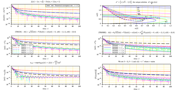
Figure 1: Convergence rates of values $f_{1}(x(t))-f(x^{*})$, of trajectories $\|x(t)-x^{*}\|_{2}$, and gradients   $\|\nabla f_{1}(x(t)\|_{2}$.

Example 2

Consider the convex function $f_{2}:{\mathbb{R}}^{2}\to{\mathbb{R}}$ defined by

$$f_{2}(x)=\frac{1}{2}(x_{1}+x_{2}-1)^{2}.$$

We have

$$\nabla f_{2}(x)=\begin{bmatrix}x_{1}+x_{2}-1\\ x_{1}+x_{2}-1\end{bmatrix}\text{ and }\nabla^{2}f_{1}(x)=\begin{bmatrix}1&1\\ 1&1\end{bmatrix}.$$

We have $S_{2}=\operatorname{argmin}f_{2}=\{(x_{1},1-x_{1}):x_{1}\in{\mathbb{R}}\}$ and $x^{*}=(\frac{1}{2},\frac{1}{2})$ is the minimum norm solution. The corresponding trajectories to the systems ${\rm(TRIGS)},{\rm(TRISHE)}$ are depicted in Figure 2.

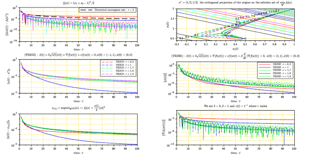
Figure 2: Convergence rates of values $f_{2}(x(t))-f(x^{*})$, trajectories $\|x(t)-x^{*}\|_{2}$, and gradients $\|\nabla f_{2}(x(t)\|_{2}$.

Example 3

To compare the systems (TRISH) and (TRISHE), we take the same function $f_{2}$ as in the previous example. The corresponding trajectories are depicted in Figure 3.

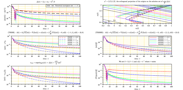
Figure 3: Comparison of (TRISH) and (TRISHE)

As predicted by the theory, it is observed that the trajectories generated by the systems (TRISH) and (TRISHE) have at the same time several remarkable properties: they ensure fast convergence of the values, fast convergence of the gradients towards zero, and convergence to the minimum norm solution. The presence of the Hessian driven damping in these dynamics induces a significant attenuation of oscillations (by comparison with (TRIGS)). The third example shows that the trajectories generated by (TRISH) and (TRISHE) share a very similar behaviour. We see the advantage of taking $r$ close to $2$ in the presence of the Hessian driven damping. Indeed, $r=2$ gives viscous damping similar to that of the accelerated gradient method of Nesterov, in which case we know that the adjustment of the coefficient $\delta$ plays a crucial role. Note the criticality of the case $r=2$, since for $r<2$ the condition for $\delta$ is $\delta>2$, whereas for $r=2$ we know that we must take $\delta\geq 3$ to get fast convergence. This is an interesting subject for further research.

5 Existence of solution trajectories for (TRISHE)

Let us start by establishing the equivalence between the inertial dynamic with Hessian driven damping (TRISHE) and a first order system in time and space in the case of a smooth function $f$. Similar result was first obtained in AABR , with applications to mechanics AMR and deep learning BCPF .

Theorem 5.1

Let $f:{\mathcal{H}}\to{\mathbb{R}}$ be a convex ${\mathcal{C}}^{2}$ function. Suppose that $\alpha\geq 0$, $\beta>0$. Let $(x_{0},\dot{x}_{0})\in{\mathcal{H}}\times{\mathcal{H}}$. The following statements are equivalent:

1. $x:[t_{0},+\infty[\to{\mathcal{H}}$ is a solution trajectory of

   $${\rm(TRISHE)}\qquad\ddot{x}(t)+\delta\sqrt{\varepsilon(t)}\dot{x}(t)+\beta\dfrac{d}{dt}\left(\nabla\varphi_{t}(x(t))\right)+\nabla\varphi_{t}(x(t))=0.$$ (84)

   with the initial conditions $x(t_{0})=x_{0}$, $\dot{x}(t_{0})=\dot{x}_{0}$.

2. $(x,y):[t_{0},+\infty[\to{\mathcal{H}}\times{\mathcal{H}}$ is a solution trajectory of the first-order system

   $$\begin{cases}\dot{x}(t)+\beta\nabla\varphi_{t}(x(t))-\left({\frac{1}{\beta}-\delta\sqrt{\varepsilon(t)}}\right)x(t)+\frac{1}{\beta}y(t)&=0\vspace{1mm}\\ \dot{y}(t)-\left({\frac{1}{\beta}-\delta\sqrt{\varepsilon(t)}-\frac{\beta\delta}{2}\frac{\dot{\epsilon}(t)}{\sqrt{\varepsilon(t)}}}\right)x(t)+\frac{1}{\beta}y(t)&=0,\end{cases}$$ (85)

with initial conditions $x(t_{0})=x_{0}$, $y(t_{0})=-\beta(\dot{x}_{0}+\beta\nabla\varphi_{t_{0}}(x_{0}))+(1-\delta\sqrt{\varepsilon(t_{0})})x_{0}$.

Proof

2. $\Rightarrow$ 1. Differentiating the first equation of (85) gives

$$\ddot{x}(t)+\beta\dfrac{d}{dt}\left(\nabla\varphi_{t}(x(t))\right)+\delta\frac{\dot{\epsilon}(t)}{2\sqrt{\varepsilon(t)}}x(t)-\left({\frac{1}{\beta}-\delta\sqrt{\varepsilon(t)}}\right)\dot{x}(t)+\frac{1}{\beta}\dot{y}(t)=0.$$ (86)

Replacing $\dot{y}(t)$ by its expression as given by the second equation of (85) gives

$$\ddot{x}(t)+\beta\dfrac{d}{dt}\left(\nabla\varphi_{t}(x(t))\right)+\delta\frac{\dot{\epsilon}(t)}{2\sqrt{\varepsilon(t)}}x(t)-\left({\frac{1}{\beta}-\delta\sqrt{\varepsilon(t)}}\right)\dot{x}(t)$$

$$+\frac{1}{\beta}\left({\left({\frac{1}{\beta}-\delta\sqrt{\varepsilon(t)}-\frac{\beta\delta}{2}\frac{\dot{\epsilon}(t)}{\sqrt{\varepsilon(t)}}}\right)x(t)-\frac{1}{\beta}y(t)}\right)=0.$$ (87)

Then replace $y(t)$ by its expression as given by the first equation of (85)

$$\ddot{x}(t)+\beta\dfrac{d}{dt}\left(\nabla\varphi_{t}(x(t))\right)+\delta\frac{\dot{\epsilon}(t)}{2\sqrt{\varepsilon(t)}}x(t)-\left({\frac{1}{\beta}-\delta\sqrt{\varepsilon(t)}}\right)\dot{x}(t)$$

$$+\frac{1}{\beta}\left({\frac{1}{\beta}-\delta\sqrt{\varepsilon(t)}-\frac{\beta\delta}{2}\frac{\dot{\epsilon}(t)}{\sqrt{\varepsilon(t)}}}\right)x(t)+\frac{1}{\beta}\left(\dot{x}(t)+\beta\nabla\varphi_{t}(x(t))-\left({\frac{1}{\beta}-\delta\sqrt{\varepsilon(t)}}\right)x(t)\right)=0.$$

After simplification of the above expression, we obtain (84).

1. $\Rightarrow$ 2. Define $y(t)$ by the first equation of (85). Differentiating $y(t)$ and using equation (84) allows one to eliminate $\ddot{x}(t)$, which finally gives the second equation of (85). ∎

Based on Theorem 5.1, the following first order formulation helps give meaning to the (TRISHE) system when $f\in\Gamma_{0}({\mathcal{H}})$. It is obtained by substituting the subdifferential $\partial\varphi_{t}$ for the gradient $\nabla\varphi_{t}$ in the first-order formulation (85).

Definition 2

Let $\delta>0$, $\beta>0$ and $f\in\Gamma_{0}({\mathcal{H}})$. Given $(x_{0},y_{0})\in{\rm dom}\kern 0.59998pt(f)\times{\mathcal{H}}$, the Cauchy problem for the inertial system (TRISHE) with generalized Hessian driven damping is defined by

$$\begin{cases}\dot{x}(t)+\beta\partial\varphi_{t}(x(t))-\left({\frac{1}{\beta}-\delta\sqrt{\varepsilon(t)}}\right)x(t)+\frac{1}{\beta}y(t)&\ni 0\\ \dot{y}(t)-\left({\frac{1}{\beta}-\delta\sqrt{\varepsilon(t)}-\frac{\beta\delta}{2}\frac{\dot{\epsilon}(t)}{\sqrt{\varepsilon(t)}}}\right)x(t)+\frac{1}{\beta}y(t)&=0\\ x(t_{0})=x_{0},y(t_{0})=y_{0}.\end{cases}$$ (88)

Let us formulate (88) in a condensed form as an evolution equation in the product space ${\mathcal{H}}\times{\mathcal{H}}$. Setting $Z(t)=(x(t),y(t))\in{\mathcal{H}}\times{\mathcal{H}}$, (88) can be equivalently written

$$\dot{Z}(t)+\partial{\mathcal{G}}(t,Z(t))+{\mathcal{D}}(t,Z(t))\ni 0,\quad{Z(t_{0})=(x_{0},y_{0})},$$ (89)

where ${\mathcal{G}}(,\cdot)\in\Gamma_{0}({\mathcal{H}}\times{\mathcal{H}})$ is the function defined by ${\mathcal{G}}(t,Z)=\beta\varphi_{t}(x)$, and the time-dependent operator ${\mathcal{D}}:\ [t_{0},+\infty[\times{\mathcal{H}}\times{\mathcal{H}}\to{\mathcal{H}}\times{\mathcal{H}}$ is given by

$${\mathcal{D}}(t,Z)=\left({-\left({\frac{1}{\beta}-\delta\sqrt{\varepsilon(t)}}\right)x+\frac{1}{\beta}y,-\left({\frac{1}{\beta}-\delta\sqrt{\varepsilon(t)}-\frac{\beta\delta}{2}\frac{\dot{\epsilon}(t)}{\sqrt{\varepsilon(t)}}}\right)x+\frac{1}{\beta}y}\right).$$ (90)

The differential inclusion (89) is governed by the sum of the time dependent maximally monotone operator $\partial{\mathcal{G}}(t,.\cdot)$ (a convex subdifferential) and the time-dependent linear continuous operator ${\mathcal{D}}(t,\cdot)$. The existence and uniqueness of a global solution for the corresponding Cauchy problem is a consequence of the general theory of evolution equations governed by maximally monotone operators (Bre1, , Proposition 3.12), and of the fact that $t\mapsto\varphi_{t}(x)$ is a nonincreasing function, see AD . In this setting, the notion of classical solution is replaced by the notion of strong solution, see (Bre1, , Definition 3.1), (APR, , Theorem 4.4), (AFK, , Theorem 2.4).

6 Conclusion, perspective

For convex optimization in Hilbert spaces, we have introduced a damped inertial dynamics which combines Hessian driven damping with Tikhonov regularization. The Hessian driven damping and the Tikhonov regularization term induce specific favorable geometric properties, related to curvature aspects. The Tikhonov term regulates the objective function. It makes the dynamic relevant of the heavy ball with friction method for a strongly convex function. The Hessian driven damping acts on the velocity vector in a similar way as continuous Newton’s method. It has a corrective effect by damping the oscillations that arise with ill-conditioned optimization problems. It turns out that the two techniques combine well and provide a substantial improvement to Nesterov’s accelerated gradient method. While preserving fast convergence of values, they ensure fast convergence of gradients to zero, they significantly reduce oscillations, and provide convergence to the minimum norm solution.

Our study provides a solid basis for the convergence analysis of algorithms obtained by temporal discretization, which is a subject of further work. Our approach calls for many developments. We showed that our approach can be naturally extended to the case of nonsmooth convex optimization, and the study of additively structured ”smooth + nonsmooth” convex optimization problems. Our study naturally leads to applications in various fields such as inverse problems for which strong convergence of trajectories, and obtaining a solution close to a desired state are key properties.

It is likely that a parallel approach can be developed for multiobjective optimization for the dynamical approach to Pareto optima, and within the framework of potential games. The Lyapunov analysis developed in this paper could also be very useful to study the asymptotic stabilization of several classes of PDE’s, for example nonlinear damped wave equations. One of the main challenges related to our study is whether similar convergence results can be obtained using autonomous systems, see ABotCest for a first systematic study of this question. Indeed the study of autonomous versions of the Tikhonov method, such as the Haugazeau method, in the context of dynamic systems, and rapid optimization, is a field largely to be explored.

Acknowledgments:

The research of Aïcha BALHAG was supported by the EIPHI Graduate School (contract ANR-17-EURE-0002).

References

- (1) B. Abbas, H. Attouch, B. F. Svaiter, Newton-like dynamics and forward-backward methods for structured monotone inclusions in Hilbert spaces, J. Optim. Theory Appl., 161 (2) (2014), 331-360.
- (2) S. Adly, H. Attouch, Van Nam Vo, Newton-type inertial algorithms for solving monotone equations governed by sums of potential and nonpotential operators, Applied Mathematics and Optimization (AMOP), 2021. hal-03260201.
- (3) F. Alvarez, H. Attouch, J. Bolte, P. Redont, A second-order gradient-like dissipative dynamical system with Hessian-driven damping. Application to optimization and mechanics, J. Math. Pures Appl., 81 (8) (2002), 747–779.
- (4) F. Alvarez, A. Cabot, Asymptotic selection of viscosity equilibria of semilinear evolution equations by the introduction of a slowly vanishing term, Discrete Contin. Dyn. Syst. 15 (2006), 921–938.
- (5) V. Apidopoulos, J.-F. Aujol, Ch. Dossal, The differential inclusion modeling the FISTA algorithm and optimality of convergence rate in the case , SIAM J. Optim., 28 (1) (2018), 551–574.
- (6) H. Attouch, Viscosity solutions of minimization problems, SIAM J. Optim. 6 (3) (1996), 769–806.
- (7) H. Attouch, A. Balhag, Z. Chbani, H. Riahi, Damped inertial dynamics with vanishing Tikhonov regularization: Strong asymptotic convergence towards the minimum norm solution, J. Differential Equations, 311 (2022), 29–58.
- (8) H. Attouch, R.I. Boţ, E.R. Csetnek, Fast optimization via inertial dynamics with closed-loop damping, Journal of the European Mathematical Society (JEMS), 2021, hal-02910307.
- (9) H. Attouch, A. Cabot, Asymptotic stabilization of inertial gradient dynamics with time-dependent viscosity, J. Differential Equations, 263 (9), (2017), 5412–5458.
- (10) H. Attouch, Z. Chbani, J. Fadili, H. Riahi, First order optimization algorithms via inertial systems with Hessian driven damping, Math. Program. (2020), https://doi.org/10.1007/s10107-020-01591-1.
- (11) H. Attouch, Z. Chbani, J. Fadili, H. Riahi, Convergence of iterates for first-order optimization algorithms with inertia and Hessian driven damping, Optimization, https://doi.org/10.1080/02331934.2021.2009828. (2021).
- (12) H. Attouch, Z. Chbani, J. Peypouquet, P. Redont, Fast convergence of inertial dynamics and algorithms with asymptotic vanishing viscosity, Math. Program., 168 (1-2) (2018), 123–175.
- (13) H. Attouch, Z. Chbani, H. Riahi, Combining fast inertial dynamics for convex optimization with Tikhonov regularization, J. Math. Anal. Appl, 457 (2018), 1065–1094.
- (14) H. Attouch, R. Cominetti, A dynamical approach to convex minimization coupling approximation with the steepest descent method, J. Differential Equations, 128 (2) (1996), 519–540.
- (15) H. Attouch, M.-O. Czarnecki, Asymptotic control and stabilization of nonlinear oscillators with non-isolated equilibria, J. Differential Equations 179 (2002), 278–310.
- (16) H. Attouch, M.-O. Czarnecki, Asymptotic behavior of coupled dynamical systems with multiscale aspects, J. Differential Equations 248 (2010), 1315–1344.
- (17) H. Attouch, M.-O. Czarnecki, Asymptotic behavior of gradient-like dynamical systems involving inertia and multiscale aspects, J. Differential Equations, 262 (3) (2017), 2745–2770.
- (18) H. Attouch, A. Damlamian, Strong solutions for parabolic variational inequalities, Nonlinear Analysis, TMA, 2 (3) (1978), 329-353.
- (19) H. Attouch, J. Fadili, From the Ravine method to the Nesterov method and vice versa: a dynamic system perspective, arXiv:2201.11643v1 [math.OC] 27 Jan 2022.
- (20) H. Attouch, J. Fadili, V. Kungurtsev, On the effect of perturbations, errors in first-order optimization methods with inertia and Hessian driven damping, arXiv:2106.16159v1 [math.OC] 30 Jun 2021.
- (21) H. Attouch, S. László, Convex optimization via inertial algorithms with vanishing Tikhonov regularization: fast convergence to the minimum norm solution, arXiv:2104.11987v1 [math.OC] 24 Apr 2021.
- (22) H. Attouch, P.E. Maingé, P. Redont, A second-order differential system with Hessian-driven damping; Application to non-elastic shock laws, Differential Equations and Applications, 4 (1) (2012), 27–65.
- (23) H. Attouch, M. Marques Alves, B.F. Svaiter, A dynamic approach to a proximal-Newton method for monotone inclusions in Hilbert Spaces, with complexity , J. of Convex Analysis, 23 (1) (2016), 139–180.
- (24) H. Attouch, J. Peypouquet, The rate of convergence of Nesterov’s accelerated forward-backward method is actually faster than , SIAM J. Optim., 26 (3) (2016), 1824–1834.
- (25) H. Attouch, J. Peypouquet, P. Redont, Fast convex minimization via inertial dynamics with Hessian driven damping, J. Differential Equations, 261 (10), (2016), 5734–5783.
- (26) H. Attouch, B. F. Svaiter, A continuous dynamical Newton-Like approach to solving monotone inclusions, SIAM J. Control Optim., 49 (2) (2011), 574–598.
- (27) J.-B. Baillon, R. Cominetti, A convergence result for non-autonomous subgradient evolution equations and its application to the steepest descent exponential penalty trajectory in linear programming, J. Funct. Anal. 187 (2001), 263–273.
- (28) H. Bauschke, P. L. Combettes, Convex Analysis and Monotone Operator Theory in Hilbert spaces, CMS Books in Mathematics, Springer, (2011).
- (29) J. Bolte, C. Castera, E. Pauwels, C. Févotte, An Inertial Newton Algorithm for Deep Learning, Journal of Machine Learning Research, 22 (2021), 1–31.
- (30) R. I. Boţ, E. R. Csetnek, S.C. László, Tikhonov regularization of a second order dynamical system with Hessian damping, Math. Program., 189 (2021), 151–186.
- (31) H. Brézis, Opérateurs maximaux monotones dans les espaces de Hilbert et équations d’évolution, Lecture Notes 5, North Holland, (1972).
- (32) H. Brézis, Analyse fonctionnelle, Masson, 1983.
- (33) A. Cabot, Inertial gradient-like dynamical system controlled by a stabilizing term, J. Optim. Theory Appl., 120 (2004), 275–303.
- (34) A. Cabot, Proximal point algorithm controlled by a slowly vanishing term: Applications to hierarchical minimization, SIAM J. Optim., 15 (2) (2005), 555–572.
- (35) A. Cabot, H. Engler, S. Gadat, On the long time behavior of second order differential equations with asymptotically small dissipation, Trans. Amer. Math. Soc., 361 (2009), 5983–6017.
- (36) A. Chambolle, Ch. Dossal, On the convergence of the iterates of Fista, J. Opt. Theory Appl., 166 (2015), 968–982.
- (37) R. Cominetti, J. Peypouquet, S. Sorin, Strong asymptotic convergence of evolution equations governed by maximal monotone operators with Tikhonov regularization, J. Differential Equations, 245 (2008), 3753–3763.
- (38) S.A. Hirstoaga, Approximation et résolution de problèmes d’équilibre, de point fixe et d’inclusion monotone. PhD thesis, Université Pierre et Marie Curie - Paris VI, 2006, HAL Id: tel-00137228.
- (39) M.A. Jendoubi, R. May, On an asymptotically autonomous system with Tikhonov type regularizing term, Archiv der Mathematik, 95 (4) (2010), 389–399.
- (40) R. May, C. Mnasri, M. Elloumi, Asymptotic for a second order evolution equation with damping and regularizing terms, AIMS Mathematics, 6 (5) (2021), 4901–4914.
- (41) Y. Nesterov, A method of solving a convex programming problem with convergence rate , Soviet Math. Dokl., 27 (1983), 372–376.
- (42) Y. Nesterov, Introductory lectures on convex optimization: A basic course, volume 87 of Applied Optimization. Kluwer Academic Publishers, Boston, MA, 2004.
- (43) Y. Nesterov, How to Make the Gradients Small, Optima 88, Mathematical Optimization Society Newsletter, May 2012.
- (44) B. Polyak, Some methods of speeding up the convergence of iteration methods, USSR Computational Mathematics and Mathematical Physics, 4 (1964), 1–17.
- (45) B. Polyak, Introduction to Optimization, New York, NY: Optimization Software-Inc, 1987.
-
(46)
W. Siegel, Accelerated first-order methods: Differential equations and Lyapunov functions,
arXiv:1903.05671v1 [math.OC], 2019. - (47) B. Shi, S.S. Du, M. I. Jordan, W. J. Su, Understanding the acceleration phenomenon via high-resolution differential equations, Math. Program. (2021). https://doi.org/10.1007/s10107-021-01681-8.
- (48) W. Su, S. Boyd, E. J. Candès, A Differential Equation for Modeling Nesterov’s Accelerated Gradient Method: Theory and Insights. J. Mach. Learn. Res., 17(153), (2016), 1–43.
- (49) A. N. Tikhonov, Doklady Akademii Nauk SSSR 151 (1963) 501–504, (Translated in ”Solution of incorrectly formulated problems and the regularization method”. Soviet Mathematics 4 (1963) 1035–1038.
- (50) A. N. Tikhonov, V. Y. Arsenin, Solutions of Ill-Posed Problems, Winston, New York, 1977.
- (51) D. Torralba, Convergence epigraphique et changements d’échelle en analyse variationnelle et optimisation, PhD thesis, Université Montpellier, 1996.
- (52) A. C. Wilson, B. Recht, M. I. Jordan, A Lyapunov analysis of momentum methods in optimization, Journal of Machine Learning Research, 22 (2021), 1–34.