Iterative Corresponding Geometry: Fusing Region and Depth for
Highly Efficient 3D Tracking of Textureless Objects

Abstract

Tracking objects in 3D space and predicting their 6DoF pose is an essential task in computer vision. State-of-the-art approaches often rely on object texture to tackle this problem. However, while they achieve impressive results, many objects do not contain sufficient texture, violating the main underlying assumption. In the following, we thus propose ICG, a novel probabilistic tracker that fuses region and depth information and only requires the object geometry. Our method deploys correspondence lines and points to iteratively refine the pose. We also implement robust occlusion handling to improve performance in real-world settings. Experiments on the YCB-Video, OPT, and Choi datasets demonstrate that, even for textured objects, our approach outperforms the current state of the art with respect to accuracy and robustness. At the same time, ICG shows fast convergence and outstanding efficiency, requiring only $1.3\,\mathrm{ms}$ per frame on a single CPU core. Finally, we analyze the influence of individual components and discuss our performance compared to deep learning-based methods. The source code of our tracker is publicly available.

1 Introduction

For many applications in robotic manipulation and augmented reality, it is essential to know the six degrees of freedom (6DoF) pose of relevant objects. To provide this information at high frequency, 3D object tracking is used. The goal is to estimate an object’s position and orientation from consecutive image frames given its 3D model. In real-world applications, occlusions, motion blur, background clutter, textureless surfaces, object symmetries, and real-time requirements remain difficult problems. Over the years many approaches have been developed [32, 72]. They can be differentiated by the use of keypoints, edges, direct optimization, deep learning, object regions, and depth images.

While methods based on keypoints [51, 41, 50, 57, 64], edges [55, 12, 17, 20], and direct optimization [56, 13, 1, 37] were very popular in the past, multiple drawbacks exist. Both keypoints and direct optimization are not suitable for textureless objects. Edge-based methods, on the other hand, typically struggle with background clutter and object texture. Further problems emerge from reflections and motion blur, which change the appearance of both texture and edges. To overcome those issues, data-driven techniques that use convolutional neural networks have been proposed [15, 67, 34, 65]. While most of those methods require significant computational resources and a detailed 3D model, they achieve promising results. For the tracking of textureless objects in cluttered environments, region-based techniques have also become very popular [59, 76, 63, 45]. Furthermore, the emergence of consumer depth sensors has enabled additional trackers that do not rely on texture [11, 27, 54, 69, 40]. Finally, while all those methods can be used independently, many approaches demonstrated the benefits of combining different techniques [47, 28, 62, 29].

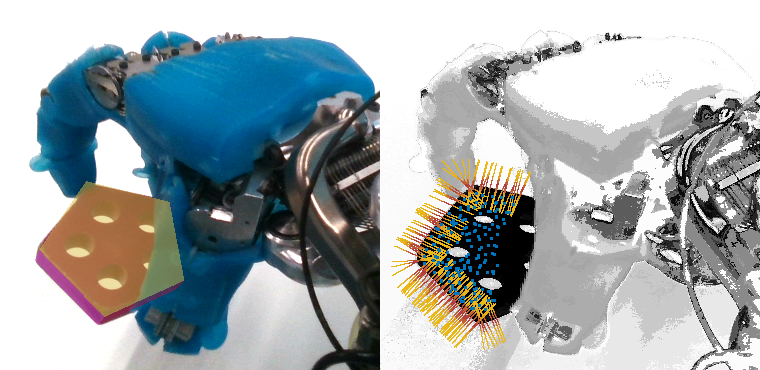
Figure 1: Tracking of a pentagon object for robotic manipulation. The image on the left shows an overlay of the object model for the predicted pose. On the right, probabilities that a pixel belongs to the background are encoded in a grayscale image. Correspondence lines are shown in yellow, with high probabilities indicated in red. Projected correspondence points are illustrated in blue.

In the past, it was shown that a combination of region and depth has great potential for the tracking of textureless objects [47, 28]. However, while region-based techniques improved greatly with respect to efficiency and quality [59, 58], no recent combined approach exists. In the following, we thus build on current developments and propose ICG, a highly efficient method that fuses geometric information from region-based correspondence lines and depth-based correspondence points. An illustration of the used correspondences is shown in Fig. 1. In a detailed evaluation on three different datasets, our method demonstrates state-of-the-art performance compared to both classical and deep learning-based techniques. In addition, given that only few such comparisons were conducted in the past, we are able to gain new insights into the current state of deep learning-based object tracking and pose estimation.

2 Related Work

In the following, we provide an overview on region-, depth-, and deep learning-based techniques. Region-based methods typically use color statistics to model the probability that a pixel belongs to the object or to the background. The object pose is then optimized to best explain the segmentation of the image. While early approaches treated segmentation and optimization separately [53, 6, 49], subsequent work [14] combined the two steps. Later, the pixel-wise posterior membership of [3] was used to develop PWP3D [45]. Based on this method, multiple combined approaches that incorporate depth information [47, 28], edges [60, 33], inertial measurements [44], or use direct optimization [36, 75, 35] were developed. In addition, it was suggested to localize the probabilistic segmentation model [23, 63, 76]. Different optimization techniques such as particle filters [74], Levenberg Marquardt [44], Gauss Newton [63], or Newton with Tikhonov regularization [58, 59] were also proposed. Finally, starting from the ideas of [28], the efficiency problem of region-based methods was addressed with the development of the sparse tracker SRT3D [58, 59].

Depth-based methods try to minimize the distance between the surface of a 3D model and measurements from a depth camera. Often, approaches based on the Iterative Closest Point (ICP) framework [9, 2] are used. While many variants exist [52, 43], all algorithms iteratively establish correspondences and minimize a respective error function. For tracking, projective data association [4] and the point-to-plane error metric [9] are very common [40, 42, 62, 28]. Apart from correspondence points and ICP, methods that utilize signed distance functions are often used [18, 48, 54, 47]. In addition, approaches that employ particle filters [69, 10, 30, 11] or robust Gaussian filters [27] instead of gradient-based optimization are also very popular.

While deep learning has proven highly successful for 6DoF pose estimation [31, 21, 66, 71, 61], pure tracking methods were only recently proposed. Many approaches are inspired by pose refinement and predict the relative pose between object renderings and subsequent images [34, 38, 67]. In addition, PoseRBPF [15] uses a Rao-Blackwellized particle filter on pose-representative latent codes [61] while 6-Pack [65] tracks anchor-based keypoints.

3 Probabilistic Model

In this section, mathematical concepts and the used notation are introduced. This is followed by an explanation of the sparse viewpoint model. Finally, the probability density functions for region and depth are derived.

3.1 Preliminaries

In this work, we use $\boldsymbol{X}=\begin{bmatrix}X&Y&Z\end{bmatrix}^{\top}\in\mathbb{R}^{3}$ and the homogeneous form $\boldsymbol{\widetilde{X}}=\begin{bmatrix}X&Y&Z&1\end{bmatrix}^{\top}$ to describe 3D model points. Image coordinates $\boldsymbol{x}=\begin{bmatrix}x&y\end{bmatrix}^{\top}\in\mathbb{R}^{2}$ are employed to access color values $\boldsymbol{y}=\boldsymbol{I}_{\textrm{c}}(\boldsymbol{x})$ and depth values $d_{Z}=I_{\textrm{d}}(\boldsymbol{x})$ from the respective color and depth images. With the pinhole camera model, a 3D model point is projected into an undistorted image as follows

$$\boldsymbol{x}=\boldsymbol{\pi}(\boldsymbol{X})=\begin{bmatrix}\frac{X}{Z}f_{x}+p_{x}\\ \frac{Y}{Z}f_{y}+p_{y}\end{bmatrix},$$ (1)

where $f_{x}$ and $f_{y}$ are the focal lengths and $p_{x}$ and $p_{y}$ are the coordinates of the principal point.

To describe the relative pose between two reference frames A and B, the homogeneous matrix ${}_{A}\boldsymbol{T}_{B}{}\in\mathbb{SE}(3)$ is used. It transforms 3D model points as follows

$$_{\textrm{A}}\boldsymbol{\widetilde{X}}={}_{\textrm{A}}\boldsymbol{T}_{\textrm{B}}{}_{\textrm{B}}\boldsymbol{\widetilde{X}}=\begin{bmatrix}{}_{\textrm{A}}\boldsymbol{R}_{\textrm{B}}&{}_{\textrm{A}}\boldsymbol{t}_{\textrm{B}}\\ \boldsymbol{0}&1\end{bmatrix}{}_{\textrm{B}}\boldsymbol{\widetilde{X}},$$ (2)

with ${}_{\textrm{A}}\boldsymbol{\widetilde{X}}$ and ${}_{\textrm{B}}\boldsymbol{\widetilde{X}}$ a point written in the coordinate frames A and B. The rotation matrix ${}_{\textrm{A}}\boldsymbol{R}_{\textrm{B}}\in\mathbb{SO}(3)$ and the translation vector ${}_{\textrm{A}}\boldsymbol{t}_{\textrm{B}}\in\mathbb{R}^{3}$ define the transformation from B to A. In this work, M, C, and D will be used to denote the model, the color camera, and the depth camera frames, respectively.

For small variations of the pose in the model reference frame M, we use the following minimal representation

$$_{\textrm{M}}\boldsymbol{\widetilde{X}}(\boldsymbol{\theta})={}_{\textrm{M}}\boldsymbol{T}(\boldsymbol{\theta}){}_{\textrm{M}}\boldsymbol{\widetilde{X}}=\begin{bmatrix}\boldsymbol{I}+[\boldsymbol{\theta}_{\textrm{r}}]_{\times}&\boldsymbol{\theta}_{\textrm{t}}\\ \boldsymbol{0}&1\end{bmatrix}{}_{\textrm{M}}\boldsymbol{\widetilde{X}},$$ (3)

where $[\boldsymbol{\theta}_{\textrm{r}}]_{\times}$ is the skew-symmetric matrix of $\boldsymbol{\theta}_{\textrm{r}}$. The vectors $\boldsymbol{\theta}_{\textrm{r}}\in\mathbb{R}^{3}$ and $\boldsymbol{\theta}_{\textrm{t}}\in\mathbb{R}^{3}$ are the rotational and translational components of the full variation vector $\boldsymbol{\theta}^{\top}=\begin{bmatrix}\boldsymbol{\theta}_{\textrm{r}}^{\top}&\boldsymbol{\theta}_{\textrm{t}}^{\top}\end{bmatrix}$.

3.2 Sparse Viewpoint Model

To ensure efficiency and avoid the rendering of the 3D model during tracking, we represent the geometry using a sparse viewpoint model [59]. In the generation process, the object is rendered from a large number of virtual cameras that are placed on the vertices of a geodesic grid all around the object. Similar to [62], image coordinates are then randomly sampled on the contour and surface of the rendered silhouette. For each coordinate, both the 3D point ${}_{\textrm{M}}\boldsymbol{X}$ and the 3D normal vector ${}_{\textrm{M}}\boldsymbol{N}$ are reconstructed. Together with the orientation that points from the camera to the model center, those vectors are stored for each viewpoint. Given a pose estimate, obtaining the contour and surface representation reduces to a search for the closest orientation vector.

3.3 Region Modality

In the following, we adopt the region-based approach of SRT3D [58, 59] and modify it to incorporate a user-defined uncertainty. In general, SRT3D considers region information sparsely along so-called correspondence lines $\boldsymbol{l}$, which cross the estimated object contour. Similar to the image function $\boldsymbol{I}_{\textrm{c}}$, correspondence lines map coordinates $r\in\mathbb{R}$ to color values $\boldsymbol{y}=\boldsymbol{l}(r)$. Each line is thereby defined by a center $\boldsymbol{c}\in\mathbb{R}^{2}$ and a normal vector $\boldsymbol{n}\in\mathbb{R}^{2}$ in image space. Both vectors are calculated by projecting a 3D contour point $\boldsymbol{X}$ and an associated 3D normal vector $\boldsymbol{N}$ from the sparse viewpoint model into the image to establish a correspondence. In order to make correspondence lines more efficient, SRT3D introduces a scale-space formulation that combines multiple pixel values $\boldsymbol{y}$ into segments $\boldsymbol{s}$. The number of pixels is thereby defined by the scale $s\in\mathbb{N}^{+}$. In addition, line coordinates $r$ are scaled and shifted to make correspondence lines independent of their orientation and sub-pixel location. An illustration is shown in Fig. 2.

Figure 2: Projection of a correspondence line from image space into scale space. The correspondence line is defined by a center $\boldsymbol{c}$ and a normal vector $\boldsymbol{n}$. Pixels along the correspondence line are combined into segments, which are illustrated in blue and yellow. The number of pixels per segment is specified by the scale $s=2$. In the visualization, the pose-dependent 3D contour point $\boldsymbol{X}(\boldsymbol{\theta})$, which is associated with the correspondence line, is also shown. It is used to compute the distance $d(\boldsymbol{\theta})$ from the estimated contour to the center $\boldsymbol{c}$. The transformation from $r$ into the scale space $r_{\textrm{s}}$ is indicated by dotted vertical lines. Note that the space is shifted by $\Delta r$ and scaled according to $s$, as well as the line angle.

Like in most region-based methods, color statistics are used to differentiate between foreground and background. The probabilities $p(\boldsymbol{y}\mid m_{\textrm{f}})$ and $p(\boldsymbol{y}\mid m_{\textrm{b}})$ are approximated using normalized color histograms. They describe the likelihood that pixel colors $\boldsymbol{y}$ are part of the foreground or background model $m_{\textrm{f}}$ or $m_{\textrm{b}}$. Based on those probabilities, segment-wise posteriors are calculated as

$$p_{\textrm{s}i}(r_{\textrm{s}})=\frac{\prod\limits_{\boldsymbol{y}\in\boldsymbol{s}}p(\boldsymbol{y}\mid m_{i})}{\prod\limits_{\boldsymbol{y}\in\boldsymbol{s}}p(\boldsymbol{y}\mid m_{\textrm{f}})+\prod\limits_{\boldsymbol{y}\in\boldsymbol{s}}p(\boldsymbol{y}\mid m_{\textrm{b}})},\quad i\in\{\textrm{f},\textrm{b}\},$$ (4)

where the segment $\boldsymbol{s}$ is defined by the coordinate $r_{\textrm{s}}$. The value describes the probability that a specific segment belongs to the foreground or background.

In addition to those measurements, theoretical probabilities that depend on the location of the object contour are developed. They are modeled by smoothed step functions

$$h_{\textrm{f}}(x) =\frac{1}{2}-\alpha_{\textrm{h}}\tanh\bigg{(}\frac{x}{2s_{\textrm{h}}}\bigg{)},$$ (5)

$$h_{\textrm{b}}(x) =\frac{1}{2}+\alpha_{\textrm{h}}\tanh\bigg{(}\frac{x}{2s_{\textrm{h}}}\bigg{)},$$ (6)

with the amplitude parameter $\alpha_{\textrm{h}}\in[0,0.5]$ and the slope parameter $s_{\textrm{h}}\in\mathbb{R}^{+}$. Using the variated 3D model point

$${}_{\textrm{C}}\boldsymbol{\widetilde{X}}(\boldsymbol{\theta})={}_{\textrm{C}}\boldsymbol{T}_{\textrm{M}}{}_{\textrm{M}}\boldsymbol{T}(\boldsymbol{\theta}){}_{\textrm{M}}\boldsymbol{\widetilde{X}},$$ (7)

the distance from the estimated contour to the correspondence line center $\boldsymbol{c}$ is approximated in scale space as follows

$$d_{\textrm{s}}(\boldsymbol{\theta})=\bigg{(}\boldsymbol{n}^{\top}\Big{(}\boldsymbol{\pi}\big{(}{}_{\textrm{C}}\boldsymbol{X}(\boldsymbol{\theta})\big{)}-\boldsymbol{c}\Big{)}-\Delta r\bigg{)}\frac{\bar{n}}{s},$$ (8)

where $\bar{n}=\lVert\boldsymbol{n}\rVert_{\mathrm{max}}$ projects to the closest horizontal or vertical image coordinate, and $\Delta r\in\mathbb{R}$ is an offset to a defined pixel location. An illustration of the transformation is shown in Fig. 2. Finally, based on those functions, SRT3D estimates the PDF for the scaled contour distance as

$$p(d_{\textrm{s}}(\boldsymbol{\theta})\mid\omega_{\textrm{s}},\boldsymbol{l})\propto\prod_{r_{\textrm{s}}\in\omega_{\textrm{s}}}\sum_{i\in\{\textrm{f},\textrm{b}\}}h_{i}\big{(}r_{\textrm{s}}-d_{\textrm{s}}(\boldsymbol{\theta})\big{)}p_{\textrm{s}i}(r_{\textrm{s}}),$$ (9)

with $\omega_{\textrm{s}}$ the considered correspondence line domain.

Note that this PDF is defined in scale space. Thanks to the proof in [58], we know that, under certain conditions, the variance of the PDF is equal to the slope parameter $s_{\textrm{h}}$ defined for the smoothed step functions $h_{\textrm{f}}$ and $h_{\textrm{b}}$. Given this variance, the expected unscaled variance in units of pixels is $\sigma^{2}=\nicefrac{{s_{\textrm{h}}s^{2}}}{{\bar{n}^{2}}}$. In contrast to previous work, we want correspondence lines to be independent of scale and slope parameters. This has the advantage that for all correspondence lines, the variance is defined in the same unit of pixels. In addition, we want to define our confidence in the region modality. Introducing the user-defined standard deviation $\sigma_{\textrm{r}}$, the PDF in Eq. 9 is thus scaled as follows

$$p(\boldsymbol{\theta}\mid\omega_{\textrm{s}},\boldsymbol{l})\propto p(d_{\textrm{s}}(\boldsymbol{\theta})\mid\omega_{\textrm{s}},\boldsymbol{l})^{\frac{s_{\textrm{h}}s^{2}}{\sigma_{\textrm{r}}^{2}\bar{n}^{2}}}.$$ (10)

The formulation helps to fuse the region modality with other information, given a defined uncertainty. Also, as shown in Appendix C, it improves results compared to SRT3D.

3.4 Depth Modality

Based on ICP [9, 2], the depth modality starts with a search for correspondence points. Similar to projective data association [4], a 3D surface point $\boldsymbol{X}$ from the sparse viewpoint model is first projected into the depth image. Given a user-defined radius and stride, multiple 3D points within a quadratic area are then reconstructed. Finally, a correspondence point $\boldsymbol{P}\in\mathbb{R}^{3}$ is selected as the point closest to the point $\boldsymbol{X}$. Correspondences with a distance bigger than a threshold are rejected. Note that techniques such as normal shooting [9, 19], and rejection strategies based on the median distance [16], the best percentage [46], and the compatibility of normal vectors [73] were also tested. However, in the end, this simple procedure worked best.

For the probabilistic model, we formulate a normal distribution that uses the point-to-plane error metric [9]. The distance between the 3D surface point $\boldsymbol{X}$ and correspondence point $\boldsymbol{P}$ is thereby calculated along the associated normal vector $\boldsymbol{N}$. Given the correspondence point $\boldsymbol{P}$, the probability for the pose variation vector $\boldsymbol{\theta}$ is written as

$$p(\boldsymbol{\theta}\mid\boldsymbol{P})\propto\exp\bigg{(}-\frac{1}{2d_{\textrm{Z}}^{2}\sigma_{\textrm{d}}^{2}}\Big{(}{}_{\textrm{M}}\boldsymbol{N}^{\top}\big{(}{}_{\textrm{M}}\boldsymbol{X}-{}_{\textrm{M}}\boldsymbol{P}(\boldsymbol{\theta})\big{)}\Big{)}^{2}\bigg{)}$$ (11)

with

$${}_{\textrm{M}}\boldsymbol{\widetilde{P}}(\boldsymbol{\theta})={}_{\textrm{M}}\boldsymbol{T}(-\boldsymbol{\theta}){}_{\textrm{M}}\boldsymbol{T}_{\textrm{D}}{}_{\textrm{D}}\boldsymbol{\widetilde{P}}.$$ (12)

Note that the user-defined standard deviation $\sigma_{\textrm{d}}$ is scaled by the depth value $d_{\textrm{Z}}$ of the correspondence point $\boldsymbol{P}$. The scaling takes into account that the number and quality of depth measurements decreases with the distance to the camera. In addition, it also ensures compatibility with the uncertainty of the region modality, which increases with the camera distance. In Eq. 11, we variate the correspondence point $\boldsymbol{P}$ instead of the model. This has the advantage that the normal vector remains fixed, and only one vector has to be variated. Based on the derived PDFs for region and depth, we can now optimize for the pose that best explains the data.

4 Optimization

In the following, we first introduce the Newton method with Tikhonov regularization that is used to maximize the probability. Subsequently, we define the gradient vector and the Hessian matrix that are required in this optimization.

4.1 Regularized Newton Method

Assuming that measurements from both modalities are independent, the joint probability function is written as

$$p(\boldsymbol{\theta}\mid\boldsymbol{\mathcal{D}})=\prod_{i=0}^{n_{\textrm{r}}}p(\boldsymbol{\theta}\mid\omega_{\textrm{s}i},\boldsymbol{l}_{i})\prod_{i=0}^{n_{\textrm{d}}}p(\boldsymbol{\theta}\mid\boldsymbol{P}_{i}),$$ (13)

with $\boldsymbol{\mathcal{D}}$ the considered data and $n_{\textrm{r}}$ and $n_{\textrm{d}}$ the number of used correspondence lines and correspondence points, respectively. The joint optimization of correspondence lines and correspondence points is visualized in Fig. 3.

Figure 3: Optimization of the corresponding geometry. For blue surface points and normal vectors, the probability given a red correspondence point is illustrated by a normal distribution. For yellow correspondence lines, the discrete distribution is illustrated. The location of 3D contour points is thereby projected to the image plane. During optimization, the joint probability is maximized.

To maximize the probability, multiple iterations, where we calculate the variation vector $\boldsymbol{\hat{\theta}}$ and update the object pose, are performed. In each iteration, the Newton method with Tikhonov regularization is used as follows

$$\boldsymbol{\hat{\theta}}=\bigg{(}-\boldsymbol{H}+\begin{bmatrix}\lambda_{\textrm{r}}\boldsymbol{I}_{3}&\boldsymbol{0}\\ \boldsymbol{0}&\lambda_{\textrm{t}}\boldsymbol{I}_{3}\end{bmatrix}\bigg{)}^{-1}\boldsymbol{g},$$ (14)

where $\boldsymbol{g}$ is the gradient vector, $\boldsymbol{H}$ the Hessian matrix, and $\lambda_{\textrm{r}}$ and $\lambda_{\textrm{t}}$ are the rotational and translational regularization parameters. The gradient vector and the Hessian matrix are thereby defined as the first- and second-order derivatives of the logarithm of the joint probability function in Eq. 13.

The big advantage of the Newton formulation is that, with the Hessian matrix, uncertainty is considered in all dimensions. This means that, in addition to weighting the two modalities with $\sigma_{\textrm{r}}$ and $\sigma_{\textrm{d}}$, it also takes into account how well each correspondence constrains the different directions. In addition, Tikhonov regularization acts as a prior probability that controls how much we believe in the previous pose. For directions with little information, this regularization helps to keep the optimization stable.

Finally, given the knowledge that $\boldsymbol{\hat{\theta}}_{\textrm{r}}$ corresponds to the rotation vector of the axis-angle representation, we are able to update the pose using the exponential map as follows

$$_{\textrm{A}}\boldsymbol{T}_{\textrm{M}}^{+}={}_{\textrm{A}}\boldsymbol{T}_{\textrm{M}}\begin{bmatrix}\exp([\boldsymbol{\hat{\theta}}_{\textrm{r}}]_{\times})&\boldsymbol{\hat{\theta}}_{\textrm{t}}\\ \boldsymbol{0}&1\end{bmatrix},\quad\textrm{A}\in\{\textrm{C},\textrm{D}\}.$$ (15)

Note that, typically, either the pose with respect to the color or the depth camera is calculated using Eq. 15. The other is then updated using the known relative transformation.

4.2 Gradient and Hessian

Because the logarithm is applied in the calculation of the gradient vector and the Hessian matrix, products turn into summations and, based on Eq. 13, we can write

$$\boldsymbol{g} =\sum_{i=1}^{n_{\textrm{r}}}\boldsymbol{g}_{\textrm{r}i}+\sum_{i=1}^{n_{\textrm{d}}}\boldsymbol{g}_{\textrm{d}i},$$ (16)

$$\boldsymbol{H} =\sum_{i=1}^{n_{\textrm{r}}}\boldsymbol{H}_{\textrm{r}i}+\sum_{i=1}^{n_{\textrm{d}}}\boldsymbol{H}_{\textrm{d}i},$$ (17)

where $\boldsymbol{g}_{\textrm{r}i}$ and $\boldsymbol{H}_{\textrm{r}i}$ are calculated from individual correspondence lines of the region modality, and $\boldsymbol{g}_{\textrm{d}i}$ and $\boldsymbol{H}_{\textrm{d}i}$ are based on correspondence points from the depth modality.

For the region modality, we apply the chain rule to calculate gradient vectors and Hessian matrices as follows

$$\boldsymbol{g}_{\textrm{r}i} =\frac{s_{\textrm{h}}s^{2}}{\sigma_{\textrm{r}}^{2}\bar{n}_{i}^{2}}\frac{\partial\ln\big{(}p(d_{\textrm{s}i}\mid\omega_{\textrm{s}i},\boldsymbol{l}_{i})\big{)}}{\partial d_{\textrm{s}i}}\frac{\partial d_{\textrm{s}i}}{\partial{}_{\textrm{C}}\boldsymbol{X}_{i}}\frac{\partial{}_{\textrm{C}}\boldsymbol{X}_{i}}{\partial\boldsymbol{\theta}}\bigg{|}_{\boldsymbol{\theta}=\boldsymbol{0}},$$ (18)

$$\begin{split}\boldsymbol{H}_{\textrm{r}i}&\approx\frac{s_{\textrm{h}}s^{2}}{\sigma_{\textrm{r}}^{2}\bar{n}_{i}^{2}}\frac{\partial^{2}\ln\big{(}p(d_{\textrm{s}i}\mid\omega_{\textrm{s}i},\boldsymbol{l}_{i})\big{)}}{\partial{d_{\textrm{s}i}}^{2}}\left(\frac{\partial d_{\textrm{s}i}}{\partial{}_{\textrm{C}}\boldsymbol{X}_{i}}\frac{\partial{}_{\textrm{C}}\boldsymbol{X}_{i}}{\partial\boldsymbol{\theta}}\right)^{\top}\\ &\hskip 35.56593pt\left(\frac{\partial d_{\textrm{s}i}}{\partial_{\textrm{C}}\boldsymbol{X}_{i}}\frac{\partial_{\textrm{C}}\boldsymbol{X}_{i}}{\partial\boldsymbol{\theta}}\right)\bigg{|}_{\boldsymbol{\theta}=\boldsymbol{0}}.\end{split}$$ (19)

Note that, similar to [58], second-order partial derivatives for $d_{\textrm{s}i}$ and ${}_{\textrm{C}}\boldsymbol{X}_{i}$ are neglected. Using Eqs. 7 and 8, the following first-order partial derivatives can be calculated

$$\begin{split}\frac{\partial d_{\textrm{s}i}}{\partial_{\textrm{C}}\boldsymbol{X}_{i}}&=\frac{\bar{n}_{i}}{s}\frac{1}{{}_{\textrm{C}}Z_{i}^{2}}\big{[}\begin{matrix}n_{xi}f_{x}{}_{\textrm{C}}Z_{i}&n_{yi}f_{y}{}_{\textrm{C}}Z_{i}\end{matrix}\\ &\hskip 49.79231pt\begin{matrix}-n_{xi}f_{x}{}_{\textrm{C}}X_{i}-n_{yi}f_{y}{}_{\textrm{C}}Y_{i}\end{matrix}\big{]},\end{split}$$ (20)

$$\frac{\partial_{\textrm{C}}\boldsymbol{X}_{i}}{\partial\boldsymbol{\theta}} ={}_{\textrm{C}}\boldsymbol{R}_{\textrm{M}}\begin{bmatrix}-[_{\textrm{M}}\boldsymbol{X}_{i}]_{\times}&\boldsymbol{I}_{3}\end{bmatrix}.$$ (21)

To estimate the first- and second-order partial derivatives for the posterior probability distribution $p(d_{\textrm{s}i}\mid\omega_{\textrm{s}i},\boldsymbol{l}_{i})$, we use the same techniques as in [59] and differentiate between global and local optimization. For global optimization, the PDF is sampled over $d_{\textrm{s}i}$, and the mean $\mu_{i}$ and variance $\sigma_{i}^{2}$ are calculated to approximate a normal distribution. Based on this normal distribution, derivatives are calculated as

$$\frac{\partial\ln\big{(}p(d_{\textrm{s}i}\mid\omega_{\textrm{s}i},\boldsymbol{l}_{i})\big{)}}{\partial{d_{\textrm{s}i}}} \approx-\frac{1}{\sigma_{i}^{2}}(d_{\textrm{s}i}-\mu_{i}),$$ (22)

$$\frac{\partial^{2}\ln\big{(}p(d_{\textrm{s}i}\mid\omega_{\textrm{s}i},\boldsymbol{l}_{i})\big{)}}{\partial{d_{\textrm{s}i}}^{2}} \approx-\frac{1}{\sigma_{i}^{2}}.$$ (23)

For local optimization, the two probability values corresponding to the discrete distances $d_{\textrm{s}i}^{-}$ and $d_{\textrm{s}i}^{+}$ closest to $d_{\textrm{s}i}$ are used to approximate first-order partial derivatives as

$$\frac{\partial\ln\big{(}p(d_{\textrm{s}i}\mid\omega_{\textrm{s}i},\boldsymbol{l}_{i})\big{)}}{\partial{d_{\textrm{s}i}}}\approx\frac{\alpha_{\textrm{s}}}{\sigma_{i}^{2}}\ln\bigg{(}\frac{p(d_{\textrm{s}i}^{+}\mid\omega_{\textrm{s}i},\boldsymbol{l}_{i}}{p(d_{\textrm{s}i}^{-}\mid\omega_{\textrm{s}i},\boldsymbol{l}_{i})}\bigg{)},$$ (24)

where $\alpha_{\textrm{s}}$ is a user-defined learning rate. Second-order partial derivatives are again calculated according to Eq. 23.

Finally, for the depth modality, gradient vectors and Hessian matrices can be calculated using Eqs. 11 and 12

$$\boldsymbol{g}_{\textrm{d}i} =-\frac{1}{d_{Z}^{2}\sigma_{d}^{2}}{}_{\textrm{M}}\boldsymbol{N}_{i}^{\top}\big{(}{}_{\textrm{M}}\boldsymbol{X}_{i}-{}_{\textrm{M}}\boldsymbol{P}_{i}\big{)}\begin{bmatrix}{}_{\textrm{M}}\boldsymbol{P}_{i}{\times}{}_{\textrm{M}}\boldsymbol{N}_{i}\\ {}_{\textrm{M}}\boldsymbol{N}_{i}\end{bmatrix},$$ (25)

$$\boldsymbol{H}_{\textrm{d}i} =-\frac{1}{d_{Z}^{2}\sigma_{d}^{2}}\begin{bmatrix}{}_{\textrm{M}}\boldsymbol{P}_{i}\times{}_{\textrm{M}}\boldsymbol{N}_{i}\\ {}_{\textrm{M}}\boldsymbol{N}_{i}\end{bmatrix}\begin{bmatrix}{}_{\textrm{M}}\boldsymbol{P}_{i}\times{}_{\textrm{M}}\boldsymbol{N}_{i}\\ {}_{\textrm{M}}\boldsymbol{N}_{i}\end{bmatrix}^{\top}.$$ (26)

5 Implementation

The following section provides implementation details, discusses how ICG can be used for pose refinement, and explains how occlusions are handled. For our implementation, we built on the code of SRT3D [59]. To generate the sparse viewpoint model, the object is rendered from $2562$ virtual cameras that are placed on a geodesic grid with a distance of $0.8\,\mathrm{m}$ to the object center. For each view, contour and surface points are sampled and normal vectors are approximated. For contour points, distances along the normal vector for which the foreground and background are not interrupted are also computed. To ensure only one transition exists on a correspondence line, lines with at least one of the two distances below $3$ segments are rejected.

The two color histograms for foreground and background are discretized by 4096 equidistant bins. In their calculation, the first 20 pixels from the line center are used. During tracking, we update histograms once the final pose was computed using the online adaptation of [3] with a learning rate of $\alpha=0.2$. In addition to tracking, our algorithm can also be used for pose refinement. In such cases, we initialize histograms at each iteration before correspondences are established. Since we do not perform a continuous update, histograms do not show the same quality as for tracking. Nevertheless, they still include useful information that helps the algorithm to converge. Experiments that demonstrate the performance for pose refinement are provided in Appendix E.

For the region modality, the probability distributions $p(d_{\textrm{s}i}\mid\omega_{\textrm{s}i},\boldsymbol{l}_{i})$ are evaluated at $12$ discrete distance values $d_{\textrm{s}i}\in\{-5.5,-4.5,\dots,5.5\}$. In the calculation of each probability value, we use $8$ precomputed values for the smoothed step functions $h_{\textrm{f}}$ and $h_{\textrm{b}}$ that correspond to $x\in\{-3.5,-2.5,\dots,3.5\}$. Also, we define the slope parameter $s_{\textrm{h}}=0.5$, the amplitude parameter $\alpha_{\textrm{h}}=0.43$, and the learning rate $\alpha_{\textrm{s}}=1.3$. To find correspondence points for the depth modality, image values on a quadratic grid with a stride of $5\,\mathrm{mm}$ and a radius equal to the correspondence threshold $r_{\textrm{t}}$ are considered. Both parameter values are projected from meters into pixels based on the depth of the 3D surface point. Correspondence points with a distance that is bigger than the threshold $r_{\textrm{t}}$ are rejected. Valid correspondences are then used in the optimization with the regularization parameters $\lambda_{\textrm{r}}=1000$ and $\lambda_{\textrm{t}}=30000$.

To find the final pose, we conduct 4 iterations in which correspondences are established. For each iteration, the standard deviations $\sigma_{\textrm{r}}$ and $\sigma_{\textrm{d}}$, the scale $s$, and the threshold $r_{\textrm{t}}$ can be adjusted. This allows to define our confidence in the data and the range in which region and depth information is considered. Many characteristics such as the resolution, depth image quality, or frame-to-frame pose difference depend on the sequence. We thus adjust the parameters for every dataset and provide them in the evaluation section. Finally, in each iteration, two optimization steps are conducted. For the region modality, global optimization is used in the first and local optimization in the second.

In many real-world cases, correspondence lines and correspondence points are subject to occlusion. Based on measurements from the depth camera and estimated positions of 3D model points, occlusions can be detected. First, the minimum depth based on $25$ depth image values within a quadratic region of $20\times 20\,\mathrm{mm}$ is computed. Similarly, during model generation, an offset between the depth of the sampled model point and the minimum depth within a quadratic region of $20\times 20\,\mathrm{mm}$ is calculated. Finally, we are able to reject correspondences for which the depth of the model point minus the precomputed offset and a user-defined threshold of $30\,\mathrm{mm}$ is smaller than the measured minimum depth. Considering a region of values makes the technique robust to missing depth measurements and large local depth differences in the object surface. In cases where depth images are not available, depth renderings can be used. An illustration of the strategy is shown in Fig. 4.

Figure 4: Visualization of the occlusion handling strategy. For each blue model point, the considered region is defined by a blue line and dotted gray cone. The lower yellow line in each cone visualizes the depth value that is calculated from the model offset, while the upper yellow line adds the user-defined threshold. Red lines indicate the minimum depth measurements from the camera. For the right point, an occlusion is detected since the red depth measurement is smaller than the expected value in yellow.

6 Evaluation

In this section, we present an extensive evaluation of our approach on the YCB-Video dataset [71], the OPT dataset [70], and the dataset of Choi [10]. We thereby evaluate the robustness, accuracy, and efficiency of ICG in comparison to the state of the art. In addition, we conduct an ablation study that demonstrates the importance of individual components. Finally, we explain limitations of our approach. Note that in Appendices B and C we present further results for the region modality and the Choi dataset. Also, in Appendices D and E, we discuss how ICG performs for pose refinement and how it compares to modern 6DoF pose estimation. Qualitative results on the YCB-Video dataset and in real-world applications can be found in the provided videos.

6.1 YCB-Video Dataset

The YCB-Video dataset [71] contains $21$ YCB objects [8] and evaluates on $12$ sequences with a total of $2949$ key frames. Because it includes additional training sequences, it is very popular with deep learning-based methods. In the evaluation, the conventional and symmetric average distance errors $e_{\textrm{ADD}}$ and $e_{\textrm{ADD{-}S}}$ [24] are calculated as

$$e_{\textrm{ADD}} =\frac{1}{n}\sum_{i=1}^{n}\big{\lVert}\big{(}{}_{\textrm{M}}\boldsymbol{\widetilde{X}}_{i}-{}_{\textrm{M}}\boldsymbol{T}_{\textrm{M}_{\textrm{gt}}}{}_{\textrm{M}}\boldsymbol{\widetilde{X}}_{i}\big{)}_{3\times 1}\big{\rVert}_{2},$$ (27)

$$e_{\textrm{ADD{-}S}} =\frac{1}{n}\sum_{i=1}^{n}\min_{j\in[n]}\big{\lVert}\big{(}{}_{\textrm{M}}\boldsymbol{\widetilde{X}}_{i}-{}_{\textrm{M}}\boldsymbol{T}_{\textrm{M}_{\textrm{gt}}}{}_{\textrm{M}}\boldsymbol{\widetilde{X}}_{j}\big{)}_{3\times 1}\big{\rVert}_{2},$$ (28)

where ${}_{\textrm{M}}\boldsymbol{T}_{\textrm{M}_{\textrm{gt}}}$ is the difference between the ground-truth and the estimated model pose, $\boldsymbol{X}_{i}$ is a vertex from the object mesh, and $n$ is the number of vertices. Based on those error metrics for a single frame, [71] reports ADD and ADD-S area under curve scores. They can be calculated as

$$s_{i}=\frac{1}{m}\sum_{j=1}^{m}\max\Big{(}1-\frac{e_{ij}}{e_{\textrm{t}}},0\Big{)},$$ (29)

with $i\in\{\textrm{ADD},\textrm{ADD{-}S}\}$, the respective frame error $e_{ij}$, the number of frames $m$, and the threshold $e_{\textrm{t}}=0.1\,\mathrm{m}$.

Results of the evaluation on the YCB-Video dataset are shown in Tab. 1.

Table 1: Results on the YCB-Video dataset [71] with ADD and ADD-S area under curve scores in percent. Except for PoseRBPF[15], results are taken from [67]. For DeepIM [34], the score over all frames was adjusted to be consistent with the evaluation of other methods. Objects with no conclusive geometry are indicated by a ^⋆ while objects with no or very little texture are marked by a ^⋄.

Approach	PoseCNN + ICP + DeepIM [71]		Wüthrich [69]		RGF [27]		DeepIM [34]		se(3)-TrackNet [67]		PoseRBPF + SDF [15]		ICG (Ours)
Initial Pose	-		Ground Truth		Ground Truth		Ground Truth		Ground Truth		PoseCNN		Ground Truth
Re-initialization	-		No		No		Yes (290)		No		Yes (2)		No
Objects	ADD	ADD-S	ADD	ADD-S	ADD	ADD-S	ADD	ADD-S	ADD	ADD-S	ADD	ADD-S	ADD	ADD-S
002_master_chef_can⋆	78.0	96.3	55.6	90.7	46.2	90.2	89.0	93.8	93.9	96.3	89.3	96.7	66.4	89.7
003_cracker_box	91.4	95.3	96.4	97.2	57.0	72.3	88.5	93.0	96.5	97.2	96.0	97.1	82.4	92.1
004_sugar_box	97.6	98.2	97.1	97.9	50.4	72.7	94.3	96.3	97.6	98.1	94.0	96.4	96.1	98.4
005_tomato_soup_can⋆	90.3	94.8	64.7	89.5	72.4	91.6	89.1	93.2	95.0	97.2	87.2	95.2	73.2	97.3
006_mustard_bottle	97.1	98.0	97.1	98.0	87.7	98.2	92.0	95.1	95.8	97.4	98.3	98.5	96.2	98.4
007_tuna_fish_can⋆	92.2	98.0	69.1	93.3	28.7	52.9	92.0	96.4	86.5	91.1	86.8	93.6	73.2	95.8
008_pudding_box	83.5	90.6	96.8	97.9	12.7	18.0	80.1	88.3	97.9	98.4	60.9	87.1	73.8	88.9
009_gelatin_box	98.0	98.5	97.5	98.4	49.1	70.7	92.0	94.4	97.8	98.4	98.2	98.6	97.2	98.8
010_potted_meat_can	82.2	90.3	83.7	86.7	44.1	45.6	78.0	88.9	77.8	84.2	76.4	83.5	93.3	97.3
011_banana⋄	94.9	97.6	86.3	96.1	93.3	97.7	81.0	90.5	94.9	97.2	92.8	97.7	95.6	98.4
019_pitcher_base⋄	97.4	97.9	97.3	97.7	97.9	98.2	90.4	94.7	96.8	97.5	97.7	98.1	97.0	98.8
021_bleach_cleanser	91.6	96.9	95.2	97.2	95.9	97.3	81.7	90.5	95.9	97.2	95.9	97.0	92.6	97.5
024_bowl⋄⋆	8.1	87.0	30.4	97.2	24.2	82.4	38.8	90.6	80.9	94.5	34.0	93.0	74.4	98.4
025_mug⋄	94.2	97.6	83.2	93.3	60.0	71.2	83.2	92.0	91.5	96.9	86.9	96.7	95.6	98.5
035_power_drill	97.2	97.9	97.1	97.8	97.9	98.3	85.4	92.3	96.4	97.4	97.8	98.2	96.7	98.5
036_wood_block	81.1	91.5	95.5	96.9	45.7	62.5	44.3	75.4	95.2	96.7	37.8	93.6	93.5	97.2
037_scissors⋄	92.7	96.0	4.2	16.2	20.9	38.6	70.3	84.5	95.7	97.5	72.7	85.5	93.5	97.3
040_large_marker⋆	88.9	98.2	35.6	53.0	12.2	18.9	80.4	91.2	92.2	96.0	89.2	97.3	88.5	97.8
051_large_clamp⋄	54.2	77.9	61.2	72.3	62.8	80.1	73.9	84.1	94.7	96.9	90.1	95.5	91.8	96.9
052_extra_large_clamp⋄	36.5	77.8	93.7	96.6	67.5	69.7	49.3	90.3	91.7	95.8	84.4	94.1	85.9	94.3
061_foam_brick⋄	48.2	97.6	96.8	98.1	70.0	86.5	91.6	95.5	93.7	96.7	96.1	98.3	96.2	98.5
All Frames	80.7	94.0	78.0	90.2	59.2	74.3	82.3	91.9	93.0	95.7	87.5	95.2	86.4	96.5

For our algorithm, we use the parameters $\sigma_{\textrm{r}}=\{25,15,10\}$, $\sigma_{\textrm{d}}=\{50,30,20\}$, $s=\{7,4,2\}$, and $r_{\textrm{t}}=\{70,50,40\}$, where values are given in units of pixels and millimeters. Our method is compared to PoseCNN [71], the particle-filter-based approaches of [69] and [27], and the current state of the art in deep learning-based 3D object tracking [34], [67], and [15]. The evaluation shows that ICG achieves state-of-the-art results with respect to the ADD-S metric, outperforming all other algorithms. For the ADD score, textureless methods have a significant disadvantage since, for some objects, the geometry is not conclusive. It is, for example, not possible to determine the rotation of a rotationally symmetric object without using texture. However, even with that handicap, ICG surpasses the texture-based approaches of PoseCNN and DeepIM. Also, it comes very close to the results of PoseRBPF. In the end, only se(3)-TrackNet is able to perform significantly better.

To utilize the full frequency of modern cameras, track multiple objects simultaneously, and save resources, efficiency is essential in real-world applications. We thus report the speed and the required hardware for all algorithms in Tab. 2.

Table 2: Average speed in frames per second and hardware requirements for the CPU and GPU. Except for PoseRBPF[15], results are taken from [67]. PoseRBPF was evaluated without SDF.

Approach	Single Core	No GPU	FPS
PoseCNN+ICP+DeepIM[71]		✗	0.1 Hz
Wüthrich[69]	✓	✓	12.9 Hz
RGF[27]	✓	✓	11.8 Hz
DeepIM[34]		✗	12.0 Hz
se(3)-TrackNet[67]		✗	90.9 Hz
PoseRBPF[15]		✗	7.6 Hz
ICG (Ours)	✓	✓	788.4 Hz

The evaluation of ICG is conducted on an Intel Xeon E5-1630 v4 CPU. In comparison, [67] used an Intel Xeon E5-1660 v3 CPU and a NVIDIA Tesla K40c GPU. The results show the outstanding efficiency of our approach. While ICG runs only on a single CPU core, it is almost one order of magnitude faster than the second-best algorithm se(3)-TrackNet, which requires a high-performance GPU.

6.2 OPT Dataset

While the YCB-Video dataset features challenging sequences in real-world environments and a large number of objects, ground truth has limited accuracy and with a large threshold $e_{\textrm{t}}=0.1\,\mathrm{m}$, the dataset mostly evaluates robustness. Also, images do not contain motion blur, favoring texture-based methods. The OPT dataset [70] nicely complements those properties. It includes $6$ objects and consists of $552$ real-world sequences with significant motion blur. Ground truth is obtained using a calibration board. For the evaluation, the area under curve of the ADD metric is used with a threshold of $r_{\textrm{t}}=0.2d$, where $d$ is the largest distance between model vertices. The final value is scaled between $0$ and $20$. Following [70], we refer to it as AUC score.

Evaluation results are reported in Tab. 3.

Table 3: Results on the OPT dataset [70]. The reported AUC scores are scaled between zero and twenty to match other evaluations. Results are taken from [70] and the respective publications.

Approach	Soda	Chest	Ironman	House	Bike	Jet	Avg.
PWP3D[45]	5.87	5.55	3.92	3.58	5.36	5.81	5.01
ElasticFusion[68]	1.90	1.53	1.69	2.70	1.57	1.86	1.87
UDP[5]	8.49	6.79	5.25	5.97	6.10	2.34	5.82
ORB-SLAM2[39]	13.44	15.53	11.20	17.28	10.41	9.93	12.97
Bugaev[7]	14.85	14.97	14.71	14.48	12.55	17.17	14.79
Tjaden[63]	8.86	11.76	11.99	10.15	11.90	13.22	11.31
Zhong[76]	9.01	12.24	11.21	13.61	12.83	15.44	12.39
Li[33]	9.00	14.92	13.44	13.60	12.85	10.64	12.41
SRT3D[59]	15.64	16.30	17.41	16.36	13.02	15.64	15.73
ICG (Ours)	15.32	15.85	17.86	17.92	16.36	15.90	16.54

For ICG, the parameters $\sigma_{\textrm{r}}=\{15,5,1.5\}$, $\sigma_{\textrm{d}}=\{35,35,25\}$, $s=\{6,4,1\}$, and $r_{\textrm{t}}=\{50,20,10\}$ are used. Also, like in [59], we constrain the rotationally symmetric soda object using $\lambda_{\textrm{r}}=70000$. In the evaluation, ICG is compared to state-of-the-art classical methods that use different sources of information, including region, edge, texture, and depth. Our approach performs best or second-best for all objects and improves on the state of the art by a significant margin.

6.3 Choi Dataset

Finally, we also want to evaluate the accuracy of our method. For this, the simulated dataset of Choi [10], which features four sequences and perfect ground truth, is used. To evaluate the accuracy, root mean square (RMS) errors in the x, y, and z directions and in the roll, pitch, and yaw angles are calculated. The rotational and translational mean over all four sequences is reported in Tab. 4.

Table 4: Mean RMS errors for translation and rotation parameters on the Choi dataset [10]. Results are from the respective papers.

Approach	Choi[10]	Krull[30]	Tan[62]	Kehl[28]	ICG (Ours)
Translation [mm]	1.36	0.82	0.10	0.51	0.04
Rotation [degree]	2.45	1.38	0.07	0.26	0.04

Detailed results are provided in Appendix B.

For our algorithm, we use the parameters $\sigma_{\textrm{r}}=\{5\}$, $\sigma_{\textrm{d}}=\{10,1\}$, $s=\{2,1\}$, and $r_{\textrm{t}}=\{10\}$. Note that since the dataset provides perfect depth and uncluttered color images, results have to be considered as an upper bound. Nevertheless, the experiments demonstrate that, with good enough data, the method is highly accurate.

6.4 Ablation Study

To demonstrate the importance of the algorithm’s components, we perform an ablation study on all three datasets. Average results of this evaluation are provided in Tab. 5.

Table 5: Ablation study on critical components of our algorithm.

Dataset	Choi[10]		OPT[70]	YCB-Video[71]
Experiment	Trans.	Rot.	AUC	ADD	ADD-S
Original	0.04	0.04	16.54	86.4	96.5
W/o Region	0.06	0.04	8.94	66.1	84.1
W/o Depth	41.65	23.39	15.88	26.6	42.8
W/o Regularization	0.04	0.04	14.48	72.0	91.5
W/o Occlusion Hand.	-	-	-	77.6	91.9

The experiments show that while the effect of the depth and region modality differs between the datasets, each modality significantly contributes to the final result. Also, we observe that while values on the Choi dataset stay the same without regularization, it is very important to the challenging sequences of the OPT and YCB-Video dataset. For the case without occlusion handling, similar results are obtained.

Finally, the convergence of our approach is evaluated in Fig. 5.

Figure 5: Convergence plot showing the final results for the YCB-Video, OPT, and Choi dataset in red, yellow, and blue, respectively.

For the YCB-Video dataset, which values robustness, the algorithm converges after only two iterations. With one additional iteration, accurate results are obtained on the Choi and OPT datasets. Independent of accuracy and robustness, fast convergence ensures that a maximum of only four iterations is sufficient to obtain excellent results.

6.5 Limitations

While ICG achieves remarkable results, some limitations remain. First, our method requires the geometry of tracked objects. Also, for the region modality, objects have to be distinguishable from the background. In addition, the depth camera has to provide reasonable measurements for the object’s surface. Another important limitation emerges if the object geometry is very similar in the vicinity of a particular pose. Naturally, using geometric information alone, it is impossible to predict the correct pose in such cases. Finally, like many conventional approaches that use line search, the algorithm has only a local view of the six-dimensional joint probability distribution. As a consequence, it is constrained by local minima with a limit to the maximum pose difference between consecutive frames.

7 Conclusion

In this work, we developed ICG, a highly efficient, textureless approach to 3D object tracking. The method fuses region and depth in a well-founded probabilistic formulation that is able to handle occlusions in a robust manner. While the overall algorithm is relatively simple and requires little computation, it performs surprisingly well on multiple datasets, outperforming the current state of the art for many cases in robustness, accuracy, and efficiency. This is even more remarkable since ICG has an inherent disadvantage in not using texture. Assuming that texture would further improve results, our evaluation suggests that deep learning-based techniques do not yet surpass classical methods. This is especially surprising since, at the expense of high computational cost and limited real-time capability, such algorithms can, in theory, directly consider all available information. As a consequence, we believe that for both classical and learning-based tracking, as well as potential combinations, there remains a large number of ideas that wait to be explored to further improve 3D object tracking.

Appendix

In the following, we first state timings for the individual steps of our algorithm. After this, the full results on the Choi dataset [10] are presented, for which a concise version was shown in the main paper. Subsequently, the developed region modality is evaluated on the RBOT dataset [63], demonstrating improved tracking success. Also, we compare to state-of-the-art 6DoF pose estimation algorithms on the YCB-Video dataset [71] and discuss the role of 3D object tracking. Finally, using predictions from modern pose estimation algorithms, we demonstrate that ICG is well-suited for highly efficient pose refinement.

Appendix A Timings

In Tab. 2, an average framerate of $788.4\,\mathrm{Hz}$ was given for the evaluation on the YCB-Video dataset [71]. This corresponds to a total duration of $1.27\,\mathrm{ms}$ per frame. Of this time, the algorithm needs $0.52\,\mathrm{ms}$ for the computation of correspondence lines, $0.58\,\mathrm{ms}$ for correspondence points, $0.09\,\mathrm{ms}$ for the calculation of gradient vectors and Hessian matrices, $0.05\,\mathrm{ms}$ for the update of color histograms, and the remaining $0.03\,\mathrm{ms}$ for other operations such as the optimization and pose update. The timings demonstrate that the region- and depth-modality are well balanced, requiring similar amounts of computation.

Appendix B Choi Dataset

In the main paper in Tab. 4, only the averages over rotational and translational RMS errors were presented for the Choi dataset [10]. For the sake of completeness, we also want to provide the full results with respect to the errors in the x, y, and z directions and in the roll, pitch, and yaw angles. The results for each of the four evaluated objects as well as the mean values are shown in Tab. 6.

Table 6: RMS errors for translation and rotation parameters on the Choi dataset [10]. Results are from the respective papers.

Approach		Choi[10]	Krull[30]	Tan[62]	Kehl[28]	ICG (Ours)
Kinect Box	X	1.84	0.83	0.15	0.76	0.05
	Y	2.23	1.67	0.19	1.09	0.11
	Z	1.36	0.79	0.09	0.38	0.03
	Roll	6.41	1.11	0.09	0.17	0.02
	Pitch	0.76	0.55	0.06	0.18	0.02
	Yaw	6.32	1.04	0.04	0.20	0.02
Milk	X	0.93	0.51	0.09	0.64	0.02
	Y	1.94	1.27	0.11	0.59	0.05
	Z	1.09	0.62	0.08	0.24	0.02
	Roll	3.83	2.19	0.07	0.41	0.06
	Pitch	1.41	1.44	0.09	0.29	0.04
	Yaw	3.26	1.90	0.06	0.42	0.06
Orange Juice	X	0.96	0.52	0.11	0.50	0.04
	Y	1.44	0.74	0.09	0.69	0.03
	Z	1.17	0.63	0.09	0.17	0.02
	Roll	1.32	1.28	0.08	0.12	0.05
	Pitch	0.75	1.08	0.08	0.20	0.03
	Yaw	1.39	1.20	0.08	0.19	0.06
Tide	X	0.83	0.69	0.08	0.34	0.02
	Y	1.37	0.81	0.09	0.49	0.03
	Z	1.20	0.81	0.07	0.18	0.01
	Roll	1.78	2.10	0.05	0.15	0.03
	Pitch	1.09	1.38	0.12	0.39	0.04
	Yaw	1.13	1.27	0.05	0.37	0.03
Mean Translation		1.36	0.82	0.10	0.51	0.04
Mean Rotation		2.45	1.38	0.07	0.26	0.04

Appendix C RBOT Dataset

In Sec. 3.3, we modified the region-based approach of SRT3D [58, 59] to be independent of the scale space and to incorporate a user-defined uncertainty. In the following, we want to show that this is not only convenient for the combination with the depth modality but that the modifications also improve tracking results. We thereby use the RBOT dataset [63] to compare our approach to the state of the art in region-based tracking as well as to additional methods that include edge information.

Table 7: Tracking success rate for all objects and scenarios on the RBOT dataset [63]. Methods that incorporate information from edges in addition to region are indicated by a ^⋆. Results are from the respective publications.

Approach	Ape	Soda	Vise	Soup	Camera	Can	Cat	Clown	Cube	Driller	Duck	Egg Box	Glue	Iron	Candy	Lamp	Phone	Squirrel	Avg.
Regular
Tjaden [63]	85.0	39.0	98.9	82.4	79.7	87.6	95.9	93.3	78.1	93.0	86.8	74.6	38.9	81.0	46.8	97.5	80.7	99.4	79.9
Zhong [76]	88.8	41.3	94.0	85.9	86.9	89.0	98.5	93.7	83.1	87.3	86.2	78.5	58.6	86.3	57.9	91.7	85.0	96.2	82.7
Huang [26]⋆	91.9	44.8	99.7	89.1	89.3	90.6	97.4	95.9	83.9	97.6	91.8	84.4	59.0	92.5	74.3	97.4	86.4	99.7	86.9
Liu [35]⋆	93.7	39.3	98.4	91.6	84.6	89.2	97.9	95.9	86.3	95.1	93.4	77.7	61.5	87.8	65.0	95.2	85.7	99.8	85.5
Li [33]⋆	92.8	42.6	96.8	87.5	90.7	86.2	99.0	96.9	86.8	94.6	90.4	87.0	57.6	88.7	59.9	96.5	90.6	99.5	85.8
Sun [60]⋆	93.0	55.2	99.3	85.4	96.1	93.9	98.0	95.6	79.5	98.2	89.7	89.1	66.5	91.3	60.6	98.6	95.6	99.6	88.1
SRT3D [59]	98.8	65.1	99.6	96.0	98.0	96.5	100.0	98.4	94.1	96.9	98.0	95.3	79.3	96.0	90.3	97.4	96.2	99.8	94.2
ICG (Ours)	98.1	66.4	99.6	96.0	97.4	96.9	100.0	98.5	94.8	97.6	98.0	95.5	80.8	95.9	91.0	97.1	96.6	99.9	94.4
Dynamic Light
Tjaden [63]	84.9	42.0	99.0	81.3	84.3	88.9	95.6	92.5	77.5	94.6	86.4	77.3	52.9	77.9	47.9	96.9	81.7	99.3	81.2
Zhong [76]	89.7	40.2	92.7	86.5	86.6	89.2	98.3	93.9	81.8	88.4	83.9	76.8	55.3	79.3	54.7	88.7	81.0	95.8	81.3
Huang [26]⋆	91.8	42.3	98.9	89.9	91.3	87.8	97.6	94.5	84.5	98.1	91.9	86.7	66.2	90.9	73.2	97.1	89.2	99.6	87.3
Liu [35]⋆	93.5	38.2	98.4	88.8	87.0	88.5	98.1	94.4	85.1	95.1	92.7	76.1	58.1	79.6	62.1	93.2	84.7	99.6	84.1
Li [33]⋆	93.5	43.1	96.6	88.5	92.8	86.0	99.6	95.5	85.7	96.8	91.1	90.2	68.4	86.8	59.7	96.1	91.5	99.2	86.7
Sun [60]⋆	93.8	55.9	99.6	85.6	97.7	93.7	97.7	96.5	78.3	98.6	91.0	91.6	72.1	90.7	63.0	98.9	94.4	100.0	88.8
SRT3D [59]	98.2	65.2	99.2	95.6	97.5	98.1	100.0	98.5	94.2	97.5	97.9	96.9	86.1	95.2	89.3	97.0	95.9	99.9	94.6
ICG (Ours)	98.4	67.0	99.5	95.7	97.6	97.5	99.8	98.6	94.9	97.5	97.4	97.1	85.5	96.0	91.5	97.7	96.2	99.9	94.9
Noise
Tjaden [63]	77.5	44.5	91.5	82.9	51.7	38.4	95.1	69.2	24.4	64.3	88.5	11.2	2.9	46.7	32.7	57.3	44.1	96.6	56.6
Zhong [76]	79.3	35.2	82.6	86.2	65.1	56.9	96.9	67.0	37.5	75.2	85.4	35.2	18.9	63.7	35.4	64.6	66.3	93.2	63.6
Huang [26]⋆	89.0	45.0	89.5	90.2	68.9	38.3	95.9	72.8	20.1	85.5	92.2	26.8	15.8	66.2	52.2	58.3	65.1	98.4	65.0
Liu [35]⋆	84.7	33.0	88.8	89.5	56.4	50.1	94.1	66.5	32.3	79.6	94.2	29.6	19.9	63.4	40.3	61.6	62.4	96.9	63.5
Li [33]⋆	89.1	44.0	91.6	89.4	75.2	62.3	98.6	77.3	41.2	81.5	91.6	54.5	31.8	65.0	46.0	78.5	69.6	97.6	71.4
Sun [60]⋆	92.5	56.2	98.0	85.1	91.7	79.0	97.7	86.2	40.1	96.6	90.8	70.2	50.9	84.3	49.9	91.2	89.4	99.4	80.5
SRT3D [59]	96.9	61.9	95.4	95.7	84.5	73.9	99.9	90.3	62.2	87.8	97.6	62.2	43.4	84.3	78.2	73.3	83.1	99.7	81.7
ICG (Ours)	98.0	64.3	95.4	95.8	84.8	74.8	99.9	90.5	61.9	88.5	97.4	63.4	45.3	84.2	81.2	74.0	84.8	99.4	82.4
Unmodeled Occlusion
Tjaden [63]	80.0	42.7	91.8	73.5	76.1	81.7	89.8	82.6	68.7	86.7	80.5	67.0	46.6	64.0	43.6	88.8	68.6	86.2	73.3
Zhong [76]	83.9	38.1	92.4	81.5	81.3	85.5	97.5	88.9	76.1	87.5	81.7	72.7	52.5	77.2	53.9	88.5	79.3	92.5	78.4
Huang [26]⋆	86.2	46.3	97.8	87.5	86.5	86.3	95.7	90.7	78.8	96.5	86.0	80.6	59.9	86.8	69.6	93.3	81.8	95.8	83.6
Liu [35]⋆	87.1	36.7	91.7	78.8	79.2	82.5	92.8	86.1	78.0	90.2	83.4	72.0	52.3	72.8	55.9	86.9	77.8	93.0	77.6
Li [33]⋆	89.3	43.3	92.2	83.1	84.1	79.0	94.5	88.6	76.2	90.4	87.0	80.7	61.6	75.3	53.1	91.1	81.9	93.4	80.3
Sun [60]⋆	91.3	56.7	97.8	82.0	92.8	89.9	96.6	92.2	71.8	97.0	85.0	84.6	66.9	87.7	56.1	95.1	89.8	98.2	85.1
SRT3D [59]	96.5	66.8	99.0	95.8	95.0	95.9	100.0	97.6	92.2	96.6	95.0	94.4	79.0	94.7	89.8	95.7	93.6	99.6	93.2
ICG (Ours)	97.3	66.3	99.3	96.0	95.0	96.5	100.0	97.7	92.9	96.4	96.1	96.5	82.1	96.1	89.7	95.8	94.2	99.2	93.7
Modeled Occlusion
Tjaden [63]	82.0	42.0	95.7	81.1	78.7	83.4	92.8	87.9	74.3	91.7	84.8	71.0	49.1	73.0	46.3	90.9	76.2	96.9	77.7
Huang [26]⋆	87.8	45.5	98.1	87.2	89.0	89.8	95.1	91.4	77.4	97.1	87.7	83.0	62.5	88.6	69.7	94.1	86.0	98.9	84.9
SRT3D [59]	97.9	68.3	99.2	95.4	96.8	96.4	99.6	98.6	93.0	96.4	96.6	96.2	82.9	95.1	91.0	96.0	94.5	99.6	94.1
ICG (Ours)	97.9	69.1	99.5	97.2	97.1	96.9	99.9	98.9	93.2	97.0	97.8	97.2	84.3	96.0	92.6	97.4	95.3	99.8	94.8

All experiments in the evaluation are performed as defined by [63]. The required translational and rotational errors are calculated as follows

$$e_{\textrm{t}}=\big{\lVert}{}_{\textrm{M}}\boldsymbol{t}_{\textrm{M}_{\textrm{gt}}}\big{\rVert}_{2},$$ (30)

$$e_{\textrm{r}}=\cos^{-1}\bigg{(}\frac{\operatorname*{trace}({}_{\textrm{M}}\boldsymbol{R}_{\textrm{M}_{\textrm{gt}}})-1}{2}\bigg{)}.$$ (31)

Based on those errors, the tracking success is calculated as the percentage of estimated poses with $e_{\textrm{t}}<5\,\mathrm{cm}$ and $e_{\textrm{r}}<5^{\circ}$. In cases of unsuccessful tracking, the algorithm is re-initialized with the ground-truth pose. For ICG, we use the same parameter values as in [59] and define a decreasing standard deviation of $\sigma_{\textrm{r}}=\{15,5,3.5,1.5\}$.

Results of the evaluation are shown in Tab. 7. The reported scores show that both SRT3D and ICG achieve significantly higher results than the remaining algorithms. However, on average, ICG performs about half a percentage point better than SRT3D. This demonstrates that setting a defined standard deviation $\sigma_{\textrm{r}}$ instead of using an implicit variance of $\sigma^{2}=\nicefrac{{s_{\textrm{h}}s^{2}}}{{\bar{n}^{2}}}$ helps to further improve results.

Appendix D 6DoF Pose Estimation

Given the strong results of modern 6DoF pose estimation methods [31, 21], the question arises whether 3D object tracking is even necessary. In order to answer this, we compare ICG with state-of-the-art pose estimation methods on the YCB-Video dataset [71]. The ADD(S) metric is thereby adopted to ensure compatibility with reported results from PVN3D [22] and FFB6D [21]. It is a combined metric that uses the ADD-S score for symmetric objects and the ADD error in all other cases.

Results of the evaluation are shown in Tab. 8.

Table 8: Comparison against state-of-the-art 6DoF pose estimation methods on the YCB-Video dataset [71] with ADD(S) and ADD-S area under curve scores in percent. Results for Augmented Autoencoders [61], CosyPose [31], and ICG were computed by us. All other values are from the respective publications. While CosyPose was trained on real data, good results can also be obtained using synthetic data alone [25]. Symmetric objects for which the ADD(S) metric reports the ADD-S instead of the ADD error are indicated by a ^⋆.

Approach	PoseCNN [71]		Augmented Autoencoders [61]		DenseFusion [66]		CosyPose [31]		PVN3D [22]		FFB6D [21]		ICG (Ours)
(Training) Data	Real RGB		3D Model		Real RGB-D		Real RGB		Real RGB-D		Real RGB-D		3D Model
Objects	ADD(S) ADD-S		ADD(S) ADD-S		ADD(S) ADD-S		ADD(S) ADD-S		ADD(S) ADD-S		ADD(S) ADD-S		ADD(S) ADD-S
002_master_chef_can	50.9	84.0	27.1	50.6	-	96.4	37.3	90.6	80.5	96.0	80.6	96.3	66.4	89.7
003_cracker_box	51.7	76.9	32.2	64.5	-	95.5	76.8	94.9	94.8	96.1	94.6	96.3	82.4	92.1
004_sugar_box	68.6	84.3	73.6	88.6	-	97.5	95.2	97.6	96.3	97.4	96.6	97.6	96.1	98.4
005_tomato_soup_can	66.0	80.9	72.3	84.4	-	94.6	90.5	94.6	88.5	96.2	89.6	95.6	73.2	97.3
006_mustard_bottle	79.9	90.2	77.5	90.9	-	97.2	92.7	96.5	96.2	97.5	97.0	97.8	96.2	98.4
007_tuna_fish_can	70.4	87.9	71.2	92.2	-	96.6	93.9	97.5	89.3	96.0	88.9	96.8	73.2	95.8
008_pudding_box	62.9	79.0	47.9	67.7	-	96.5	93.5	96.2	95.7	97.1	94.6	97.1	73.8	88.9
009_gelatin_box	75.2	87.1	74.8	82.9	-	98.1	94.1	96.1	96.1	97.7	96.9	98.1	97.2	98.8
010_potted_meat_can	59.6	78.5	53.6	63.3	-	91.3	75.9	84.0	88.6	93.3	88.1	94.7	93.3	97.3
011_banana	72.3	85.9	13.1	51.6	-	96.6	90.0	95.6	93.7	96.6	94.9	97.2	95.6	98.4
019_pitcher_base	52.5	76.8	77.6	91.7	-	97.1	94.0	97.3	96.5	97.4	96.9	97.6	97.0	98.8
021_bleach_cleanser	50.5	71.9	42.0	62.6	-	95.8	82.1	92.7	93.2	96.0	94.8	96.8	92.6	97.5
024_bowl⋆	69.7	69.7	79.1	79.1	-	88.2	87.8	87.8	90.2	90.2	96.3	96.3	98.4	98.4
025_mug	57.7	78.0	58.0	80.9	-	97.1	87.8	94.9	95.4	97.6	94.2	97.3	95.6	98.5
035_power_drill	55.1	72.8	61.2	77.9	-	96.0	89.7	95.1	95.1	96.7	95.9	97.2	96.7	98.5
036_wood_block⋆	65.8	65.8	55.2	55.2	-	89.7	80.5	80.5	90.4	90.4	92.6	92.6	97.2	97.2
037_scissors	35.8	56.2	0.8	7.0	-	95.2	67.6	81.5	92.7	96.7	95.7	97.7	93.5	97.3
040_large_marker	58.0	71.4	55.6	67.6	-	97.5	84.3	93.1	91.8	96.7	89.1	96.6	88.5	97.8
051_large_clamp⋆	49.9	49.9	72.2	72.2	-	72.9	91.3	91.3	93.6	93.6	96.8	96.8	96.9	96.9
052_extra_large_clamp⋆	47.0	47.0	59.5	59.5	-	69.8	75.7	75.7	88.4	88.4	96.0	96.0	94.3	94.3
061_foam_brick⋆	87.8	87.8	56.2	56.2	-	92.5	94.7	94.7	96.8	96.8	97.3	97.3	98.5	98.5
All Frames	60.0	75.9	57.5	72.8	-	93.1	83.8	92.6	91.8	95.5	92.7	96.6	87.9	96.5

Table 9: Refined and unrefined results on the YCB-Video dataset [71] with ADD and ADD-S area under curve scores in percent. For PoseCNN with multi-hypothesis ICP, results are taken from the corresponding publication [71]. To evaluate the refinement, predicted poses for PoseCNN [71] are taken from the YCB_Video_toolbox while results for Augmented Autoencoders [61] and CosyPose [31] are computed using source code from the respective repositories.

Approach	PoseCNN [71]		PoseCNN [71]				Augmented Autoencoders [61]				CosyPose [31]
Refinement	MH ICP		-		ICG (Ours)		-		ICG (Ours)		Iterative Matching		IM + ICG (Ours)
Objects	ADD	ADD-S	ADD	ADD-S	ADD	ADD-S	ADD	ADD-S	ADD	ADD-S	ADD	ADD-S	ADD	ADD-S
002_master_chef_can	69.0	95.8	50.0	84.6	66.7	94.7	27.1	50.6	38.3	67.2	37.3	90.6	38.6	93.1
003_cracker_box	80.7	91.8	53.0	77.5	67.8	85.6	32.2	64.5	43.8	71.6	76.8	94.9	81.4	97.9
004_sugar_box	97.2	98.2	68.3	84.5	91.9	96.3	73.6	88.6	85.2	94.9	95.2	97.6	95.8	98.2
005_tomato_soup_can	81.6	94.5	66.1	81.4	82.8	91.3	72.3	84.4	82.3	90.0	90.5	94.6	92.6	95.9
006_mustard_bottle	97.0	98.4	80.8	91.1	93.9	97.4	77.5	90.9	87.9	96.9	92.7	96.5	96.3	98.4
007_tuna_fish_can	83.1	97.1	70.5	88.4	82.2	93.5	71.2	92.2	78.6	95.2	93.9	97.5	92.2	95.6
008_pudding_box	96.6	97.9	62.2	79.3	72.3	85.1	47.9	67.7	58.6	81.7	93.5	96.2	81.9	91.6
009_gelatin_box	98.2	98.8	74.9	87.7	95.1	97.8	74.8	82.9	81.9	88.9	94.1	96.1	93.5	97.9
010_potted_meat_can	83.8	92.8	59.3	78.8	69.1	82.4	53.6	63.3	61.7	68.0	75.9	84.0	78.8	85.7
011_banana	91.6	96.9	72.3	86.3	80.4	92.0	13.1	51.6	18.2	60.1	90.0	95.6	95.2	98.2
019_pitcher_base	96.7	97.8	52.9	77.6	85.9	93.6	77.6	91.7	92.1	98.0	94.0	97.3	96.7	98.7
021_bleach_cleanser	92.3	96.8	50.2	71.7	74.7	87.6	42.0	62.6	54.4	70.9	82.1	92.7	90.0	97.8
024_bowl	17.5	78.3	3.0	69.6	5.5	78.0	17.3	79.1	19.6	79.5	34.5	87.8	36.6	89.8
025_mug	81.4	95.1	58.4	78.8	88.2	96.6	58.0	80.9	82.8	93.6	87.8	94.9	94.9	98.2
035_power_drill	96.9	98.0	55.2	73.2	95.1	97.9	61.2	77.9	81.9	89.3	89.7	95.1	96.2	98.3
036_wood_block	79.2	90.5	26.4	64.3	35.5	69.9	1.6	55.2	2.5	60.8	24.8	80.5	29.0	87.4
037_scissors	78.4	92.2	34.8	55.9	59.0	79.6	0.8	7.0	0.7	7.5	67.6	81.5	73.9	86.9
040_large_marker	85.4	97.2	58.2	71.9	83.6	95.3	55.6	67.6	65.9	75.7	84.3	93.1	90.8	97.5
051_large_clamp	52.6	75.4	24.6	50.1	50.7	74.0	32.8	72.2	41.2	83.3	40.1	91.3	40.8	94.6
052_extra_large_clamp	28.7	65.3	16.3	44.5	25.8	67.7	26.9	59.5	32.5	63.6	40.2	75.7	40.5	75.1
061_foam_brick	48.3	97.1	40.4	88.2	42.2	92.5	19.4	56.2	22.5	57.7	51.7	94.7	52.7	97.6
All Frames	79.3	93.0	53.7	76.3	73.1	89.3	50.5	72.8	61.2	80.3	76.1	92.6	78.9	94.7

The comparison demonstrates that ICG is able to outperform most methods by a considerable margin for the ADD-S score, performing on par with the best reported results from FFB6D. This is remarkable since FFB6D trains on large amounts of pose-annotated real-world data that originates from a similar pose distribution. For many applications, such data is not available. In contrast, ICG only requires a texture-less 3D model and no training data. With respect to the ADD(S) metric, both PVN3D and FFB6D report better results. The main reason for this is that our method is by design not considering texture and thus has a considerable disadvantage if the geometry is not conclusive. However, in return, there is no need for textured 3D models, which are required for all competing methods.

In contrast to 6DoF pose estimation algorithms, ICG considers the pose on a frame-to-frame basis without re-initialization. This leads to a small number of objects that get stuck in local minima and thus show relatively poor performance. On the other hand, ICG benefits from temporal consistency and performs more accurate than FFB6D for most objects. The advantage of our tracker becomes particularly obvious when comparing the required computation. While FFB6D depends on a high-end GPU and reports a runtime of $75\,\mathrm{ms}$ [21], ICG requires only $1.3\,\mathrm{ms}$ per frame on a single CPU core, which is $57\times$ faster. This is especially crucial in reactive, real-time applications for which hardware constraints exist. In conclusion, the experiment demonstrates that while tracking by detection is possible, for many real-world applications, it is not the most sensible solution. Given the high efficiency and good performance of ICG, in our opinion, it is best to rely on continuous 3D tracking for local pose updates while using 6DoF pose estimation for global initialization and long-term consistency.

Appendix E 6-DoF Pose Refinement

Given that ICG is a local optimization method, the question emerges how well it would work for pose refinement. In the following, we thus use ICG to improve the predictions of PoseCNN, Augmented Autoencoders, and CosyPose and compare results on the YCB-Video dataset [71]. Depending on the pose estimation algorithm, errors along the principal axis are relatively large. To cope with those larger translational errors, we use the following parameters $r_{\textrm{t}}=\{300,250,100\}$, $\sigma_{\textrm{d}}=\{100,50,20\}$, $\lambda_{\textrm{t}}=100$, and conduct $7$ instead of $4$ iterations. For efficiency, strides are increased from $5\,\mathrm{mm}$ to $10\,\mathrm{mm}$. All other parameters remain the same as in the evaluation of tracking. With the increased number of iterations and considered area, the runtime increases to $2.7\,\mathrm{ms}$ per frame.

Results of the conducted evaluation are shown in Tab. 9. We thereby report both refined and unrefined scores for the considered 6DoF pose estimation methods. In addition, results from [71] are provided, which were obtained using an extensive multi-hypothesis ICP approach on the predictions of PoseCNN. According to [66], this refinement algorithm requires more than $10\,\mathrm{s}$ for a single pose. The evaluation shows that, even for the very good results of CosyPose, ICG is able to improve pose estimations for almost all objects. Also, it is interesting to see that, while it can not fully compete with extensive multi-hypothesis ICP refinement, the difference is not as big as one might expect. This is especially impressive considering that ICG is more than three orders of magnitude faster.

Finally, we want to ensure that the pose refinement uses both depth and region information and that improvements are not only from the ICP-based depth modality. We thus conducted a short ablation study, for which results are shown in Tab. 10.

Table 10: Ablation study comparing refined results for ICG with and without the region modality to unrefined results. Values show ADD and ADD-S area under curve scores over all frames on the YCB-Video dataset [71] in percent.

Approach	PoseCNN [71]		Augmented Autoencoders [61]		CosyPose [31]
Refinement	ADD	ADD-S	ADD	ADD-S	ADD	ADD-S
Unrefined	53.7	76.3	50.5	72.8	76.1	92.6
ICG w/o Region	65.0	84.2	57.5	76.9	76.8	93.3
ICG w/ Region	73.1	89.3	61.2	80.3	78.9	94.7

The obtained scores demonstrate that ICG is not just a blown-up ICP approach but that the addition of region information significantly helps to improve performance. Given the good pose predictions and computational efficiency, we are thus confident that, while ICG is an excellent 3D object tracking approach, it also has many applications in pose refinement.

References

- [1] Selim Benhimane and Ezio Malis. Real-time image-based tracking of planes using efficient second-order minimization. In IEEE/RSJ International Conference on Intelligent Robots and Systems, volume 1, pages 943–948, 2004.
- [2] Paul J. Besl and Neil D. McKay. A method for registration of 3-D shapes. IEEE Transactions on Pattern Analysis and Machine Intelligence, 14(2):239–256, 1992.
- [3] Charles Bibby and Ian Reid. Robust real-time visual tracking using pixel-wise posteriors. In European Conference on Computer Vision, pages 831–844, 2008.
- [4] Gérard Blais and Martin D. Levine. Registering multiview range data to create 3D computer objects. IEEE Transactions on Pattern Analysis and Machine Intelligence, 17(8):820–824, 1995.
- [5] Eric Brachmann, Frank Michel, Alexander Krull, Michael Y. Yang, Stefan Gumhold, and Carsten Rother. Uncertainty-driven 6D pose estimation of objects and scenes from a single RGB image. In IEEE Conference on Computer Vision and Pattern Recognition, pages 3364–3372, 2016.
- [6] Thomas Brox, Bodo Rosenhahn, Juergen Gall, and Daniel Cremers. Combined region and motion-based 3D tracking of rigid and articulated objects. IEEE Transactions on Pattern Analysis and Machine Intelligence, 32(3):402–415, 2010.
- [7] Bogdan Bugaev, Anton Kryshchenko, and Roman Belov. Combining 3D model contour energy and keypoints for object tracking. In European Conference on Computer Vision, pages 55–70, 2018.
- [8] Berk Calli, Arjun Singh, Aaron Walsman, Siddhartha Srinivasa, Pieter Abbeel, and Aaron M. Dollar. The YCB object and model set: Towards common benchmarks for manipulation research. In International Conference on Advanced Robotics, pages 510–517, 2015.
- [9] Yang Chen and Gérard Medioni. Object modelling by registration of multiple range images. Image and Vision Computing, 10(3):145–155, 1992.
- [10] Changhyun Choi and Henrik I. Christensen. RGB-D object tracking: A particle filter approach on GPU. In IEEE/RSJ International Conference on Intelligent Robots and Systems, pages 1084–1091, 2013.
- [11] Cristina G. Cifuentes, Jan Issac, Manuel Wüthrich, Stefan Schaal, and Jeannette Bohg. Probabilistic articulated real-time tracking for robot manipulation. IEEE Robotics and Automation Letters, 2(2):577–584, 2017.
- [12] Andrew I. Comport, Eric Marchand, Muriel Pressigout, and Francois Chaumette. Real-time markerless tracking for augmented reality: The virtual visual servoing framework. IEEE Transactions on Visualization and Computer Graphics, 12(4):615–628, 2006.
- [13] Alberto Crivellaro and Vincent Lepetit. Robust 3D tracking with descriptor fields. In IEEE Conference on Computer Vision and Pattern Recognition, pages 3414–3421, 2014.
- [14] Samuel Dambreville, Romeil Sandhu, Anthony Yezzi, and Allen Tannenbaum. Robust 3D pose estimation and efficient 2D region-based segmentation from a 3D shape prior. In European Conference on Computer Vision, pages 169–182, 2008.
- [15] Xinke Deng, Arsalan Mousavian, Yu Xiang, Fei Xia, Timothy Bretl, and Dieter Fox. PoseRBPF: A Rao–Blackwellized particle filter for 6-D object pose tracking. IEEE Transactions on Robotics, 37(5):1328–1342, 2021.
- [16] James Diebel, Kjell Reutersward, Sebastian Thrun, James Davis, and Rakesh Gupta. Simultaneous localization and mapping with active stereo vision. In IEEE/RSJ International Conference on Intelligent Robots and Systems, volume 4, pages 3436–3443, 2004.
- [17] Tom Drummond and Roberto Cipolla. Real-time visual tracking of complex structures. IEEE Transactions on Pattern Analysis and Machine Intelligence, 24(7):932–946, 2002.
- [18] Andrew W. Fitzgibbon. Robust registration of 2D and 3D point sets. Image and Vision Computing, 21(13-14):1145–1153, 2003.
- [19] Hervé Gagnon, Marc Soucy, Robert Bergevin, and Denis Laurendeau. Registration of multiple range views for automatic 3-d model building. In IEEE Conference on Computer Vision and Pattern Recognition, pages 581–586, 1994.
- [20] Chris Harris and Carl Stennett. RAPID - A video rate object tracker. In Proceedings of the British Machine Vision Conference, pages 15.1–15.6, 1990.
- [21] Yisheng He, Haibin Huang, Haoqiang Fan, Qifeng Chen, and Jian Sun. FFB6D: A full flow bidirectional fusion network for 6D pose estimation. In IEEE/CVF Conference on Computer Vision and Pattern Recognition, pages 3003–3013, 2021.
- [22] Yisheng He, Wei Sun, Haibin Huang, Jianran Liu, Haoqiang Fan, and Jian Sun. PVN3D: a deep point-wise 3D keypoints voting network for 6DoF pose estimation. In IEEE/CVF Conference on Computer Vision and Pattern Recognition (CVPR), pages 11629–11638, 2020.
- [23] Jonathan Hexner and Rami R. Hagege. 2D-3D pose estimation of heterogeneous objects using a region based approach. International Journal of Computer Vision, 118(1):95–112, 2016.
- [24] Stefan Hinterstoisser, Vincent Lepetit, Slobodan Ilic, Stefan Holzer, Gary Bradski, Kurt Konolige, and Nassir Navab. Model based training, detection and pose estimation of texture-less 3D objects in heavily cluttered scenes. In Asian Conference on Computer Vision, pages 548–562, 2013.
- [25] Tomáš Hodaň, Martin Sundermeyer, Bertram Drost, Yann Labbé, Eric Brachmann, Frank Michel, Carsten Rother, and Jiří Matas. Bop challenge 2020 on 6d object localization. In Computer Vision – ECCV 2020 Workshops, pages 577–594, 2020.
- [26] Hong Huang, Fan Zhong, Yuqing Sun, and Xueying Qin. An occlusion-aware edge-based method for monocular 3d object tracking using edge confidence. Computer Graphics Forum, 39(7):399–409, 2020.
- [27] Jan Issac, Manuel Wüthrich, Cristina G. Cifuentes, Jeannette Bohg, Sebastian Trimpe, and Stefan Schaal. Depth-based object tracking using a robust gaussian filter. In IEEE International Conference on Robotics and Automation, pages 608–615, 2016.
- [28] Wadim Kehl, Federico Tombari, Slobodan Ilic, and Nassir Navab. Real-time 3D model tracking in color and depth on a single CPU core. In IEEE Conference on Computer Vision and Pattern Recognition, pages 465–473, 2017.
- [29] Michael Krainin, Peter Henry, Xiaofeng Ren, and Dieter Fox. Manipulator and object tracking for in-hand 3D object modeling. International Journal of Robotics Research, 30(11):1311–1327, 2011.
- [30] Alexander Krull, Frank Michel, Eric Brachmann, Stefan Gumhold, Stephan Ihrke, and Carsten Rother. 6-DOF model based tracking via object coordinate regression. In Asian Conference on Computer Vision, pages 384–399, 2015.
- [31] Yann Labbé, Justin Carpentier, Mathieu Aubry, and Josef Sivic. CosyPose: Consistent multi-view multi-object 6D pose estimation. In European Conference on Computer Vision, pages 574–591, 2020.
- [32] Vincent Lepetit and Pascal Fua. Monocular Model-Based 3D Tracking of Rigid Objects: A Survey, volume 1. Foundations and Trends in Computer Graphics and Vision, 2005.
- [33] Jia-Chen Li, Fan Zhong, Song-Hua Xu, and Xue-Ying Qin. 3D object tracking with adaptively weighted local bundles. Journal of Computer Science and Technology, 36(3):555–571, 2021.
- [34] Yi Li, Gu Wang, Xiangyang Ji, Yu Xiang, and Dieter Fox. DeepIM: Deep iterative matching for 6D pose estimation. In European Conference on Computer Vision, pages 695–711, 2018.
- [35] Fulin Liu, Zhenzhong Wei, and Guangjun Zhang. An off-board vision system for relative attitude measurement of aircraft. IEEE Transactions on Industrial Electronics, 69(4):4225–4233, 2021.
- [36] Yang Liu, Pansiyu Sun, and Akio Namiki. Target tracking of moving and rotating object by high-speed monocular active vision. IEEE Sensors Journal, 20(12):6727–6744, 2020.
- [37] Bruce D. Lucas and Takeo Kanade. An iterative image registration technique with an application to stereo vision. In Proceedings of the 7th International Joint Conference on Artificial Intelligence, volume 2, pages 674–679, 1981.
- [38] Fabian Manhardt, Wadim Kehl, Nassir Navab, and Federico Tombari. Deep model-based 6D pose refinement in RGB. In European Conference on Computer Vision, pages 833–849, 2018.
- [39] Raul Mur-Artal and Juan D. Tardós. ORB-SLAM2: An open-source SLAM system for monocular, stereo, and RGB-D cameras. IEEE Transactions on Robotics, 33(5):1255–1262, 2017.
- [40] Richard A. Newcombe, Andrew J. Davison, Shahram Izadi, Pushmeet Kohli, Otmar Hilliges, Jamie Shotton, David Molyneaux, Steve Hodges, David Kim, and Andrew Fitzgibbon. KinectFusion: Real-time dense surface mapping and tracking. In IEEE International Symposium on Mixed and Augmented Reality, pages 127–136, 2011.
- [41] Mustafa Özuysal, Vincent Lepetit, François Fleuret, and Pascal Fua. Feature harvesting for tracking-by-detection. In Aleš Leonardis, Horst Bischof, and Axel Pinz, editors, European Conference on Computer Vision, pages 592–605, 2006.
- [42] Karl Pauwels, Vladimir Ivan, Eduardo Ros, and Sethu Vijayakumar. Real-time object pose recognition and tracking with an imprecisely calibrated moving rgb-d camera. In IEEE/RSJ International Conference on Intelligent Robots and Systems, pages 2733–2740, 2014.
- [43] François Pomerleau, Francis Colas, and Roland Siegwart. A review of point cloud registration algorithms for mobile robotics. Foundations and Trends in Robotics, 4(1):1–104, 2015.
- [44] Victor A. Prisacariu, Olaf Kähler, David W. Murray, and Ian D. Reid. Real-time 3D tracking and reconstruction on mobile phones. IEEE Transactions on Visualization and Computer Graphics, 21(5):557–570, 2015.
- [45] Victor A. Prisacariu and Ian D. Reid. PWP3D: Real-time segmentation and tracking of 3D objects. International Journal of Computer Vision, 98(3):335–354, 2012.
- [46] Kari Pulli. Multiview registration for large data sets. In Second International Conference on 3-D Digital Imaging and Modeling, pages 160–168, 1999.
- [47] Carl Y. Ren, Victor A. Prisacariu, Olaf Kähler, Ian D. Reid, and David W. Murray. Real-time tracking of single and multiple objects from depth-colour imagery using 3D signed distance functions. International Journal of Computer Vision, 124(1):80–95, 2017.
- [48] Carl Y. Ren and Ian Reid. A unified energy minimization framework for model fitting in depth. In Andrea Fusiello, Vittorio Murino, and Rita Cucchiara, editors, Computer Vision – ECCV 2012. Workshops and Demonstrations, pages 72–82, 2012.
- [49] Bodo Rosenhahn, Thomas Brox, and Joachim Weickert. Three-dimensional shape knowledge for joint image segmentation and pose tracking. International Journal of Computer Vision, 73(3):243–262, 2007.
- [50] Edward Rosten and Tom Drummond. Fusing points and lines for high performance tracking. In IEEE International Conference on Computer Vision, volume 2, pages 1508–1515, 2005.
- [51] Ethan Rublee, Vincent Rabaud, Kurt Konolige, and Gary Bradski. ORB: An efficient alternative to SIFT or SURF. In IEEE International Conference on Computer Vision, pages 2564–2571, 2011.
- [52] Szymon Rusinkiewicz and Marc Levoy. Efficient variants of the ICP algorithm. In Third International Conference on 3-D Digital Imaging and Modeling, pages 145–152, 2001.
- [53] Christian Schmaltz, Bodo Rosenhahn, Thomas Brox, and Joachim Weickert. Region-based pose tracking with occlusions using 3D models. Machine Vision and Applications, 23(3):557–577, 2012.
- [54] Tanner Schmidt, Richard Newcombe, and Dieter Fox. Dart: dense articulated real-time tracking with consumer depth cameras. Autonomous Robots, 39(3):239–258, 2015.
- [55] Byung-Kuk Seo, Hanhoon Park, Jong-Il Park, Stefan Hinterstoisser, and Slobodan Ilic. Optimal local searching for fast and robust textureless 3D object tracking in highly cluttered backgrounds. IEEE Transactions on Visualization and Computer Graphics, 20(1):99–110, 2014.
- [56] Byung-Kuk Seo and Harald Wuest. A direct method for robust model-based 3D object tracking from a monocular RGB image. In European Conference on Computer Vision Workshop, pages 551–562, 2016.
- [57] Iryna Skrypnyk and David G. Lowe. Scene modelling, recognition and tracking with invariant image features. In Third IEEE and ACM International Symposium on Mixed and Augmented Reality, pages 110–119, 2004.
- [58] Manuel Stoiber, Martin Pfanne, Klaus H. Strobl, Rudolph Triebel, and Alin Albu-Schaeffer. A sparse gaussian approach to region-based 6DoF object tracking. In Asian Conference on Computer Vision, pages 666–682, 2020.
- [59] Manuel Stoiber, Martin Pfanne, Klaus H. Strobl, Rudolph Triebel, and Alin Albu-Schaeffer. SRT3D: A sparse region-based 3D object tracking approach for the real world. International Journal of Computer Vision, 2022.
- [60] Xiaoliang Sun, Jiexin Zhou, Wenlong Zhang, Zi Wang, and Qifeng Yu. Robust monocular pose tracking of less-distinct objects based on contour-part model. IEEE Transactions on Circuits and Systems for Video Technology, 31(11):4409–4421, 2021.
- [61] Martin Sundermeyer, Zoltan-Csaba Marton, Maximilian Durner, Manuel Brucker, and Rudolph Triebel. Implicit 3D orientation learning for 6D object detection from RGB images. In European Conference on Computer Vision, pages 712–729, 2018.
- [62] David J. Tan, Nassir Navab, and Federico Tombari. Looking beyond the simple scenarios: Combining learners and optimizers in 3D temporal tracking. IEEE Transactions on Visualization and Computer Graphics, 23(11):2399–2409, 2017.
- [63] Henning Tjaden, Ulrich Schwanecke, Elmar Schömer, and Daniel Cremers. A region-based Gauss-Newton approach to real-time monocular multiple object tracking. IEEE Transactions on Pattern Analysis and Machine Intelligence, 41(8):1797–1812, 2018.
- [64] Luca Vacchetti, Vincent Lepetit, and Pascal Fua. Stable real-time 3D tracking using online and offline information. IEEE Transactions on Pattern Analysis and Machine Intelligence, 26(10):1385–1391, 2004.
- [65] Chen Wang, Roberto Martín-Martín, Danfei Xu, Jun Lv, Cewu Lu, Li Fei-Fei, Silvio Savarese, and Yuke Zhu. 6-PACK: Category-level 6D pose tracker with anchor-based keypoints. In IEEE International Conference on Robotics and Automation, pages 10059–10066, 2020.
- [66] Chen Wang, Danfei Xu, Yuke Zhu, Roberto Martín-Martín, Cewu Lu, Li Fei-Fei, and Silvio Savarese. DenseFusion: 6D object pose estimation by iterative dense fusion. In IEEE/CVF Conference on Computer Vision and Pattern Recognition, pages 3338–3347, 2019.
- [67] Bowen Wen, Chaitanya Mitash, Baozhang Ren, and Kostas E. Bekris. se(3)-TrackNet: Data-driven 6D pose tracking by calibrating image residuals in synthetic domains. In IEEE/RSJ International Conference on Intelligent Robots and Systems, pages 10367–10373, 2020.
- [68] Thomas Whelan, Stefan Leutenegger, Renato S. Moreno, Ben Glocker, and Andrew Davison. ElasticFusion: Dense SLAM without a pose graph. In Robotics: Science and Systems, 2015.
- [69] Manuel Wüthrich, Peter Pastor, Mrinal Kalakrishnan, Jeannette Bohg, and Stefan Schaal. Probabilistic object tracking using a range camera. In IEEE/RSJ International Conference on Intelligent Robots and Systems, pages 3195–3202, 2013.
- [70] Po-Chen Wu, Yueh-Ying Lee, Hung-Yu Tseng, Hsuan-I Ho, Ming-Hsuan Yang, and Shao-Yi Chien. A benchmark dataset for 6DoF object pose tracking. In IEEE International Symposium on Mixed and Augmented Reality, pages 186–191, 2017.
- [71] Yu Xiang, Tanner Schmidt, Venkatraman Narayanan, and Dieter Fox. PoseCNN: A convolutional neural network for 6D object pose estimation in cluttered scenes. In Robotics: Science and Systems, 2018.
- [72] Alper Yilmaz, Omar Javed, and Mubarak Shah. Object tracking: A survey. ACM Computing Surveys, 38(4):13, 2006.
- [73] Zhengyou Zhang. Iterative point matching for registration of free-form curves and surfaces. International Journal of Computer Vision, 13(2):119–152, 1994.
- [74] Song Zhao, Lingfeng Wang, Wei Sui, Huai-yu Wu, and Chunhong Pan. 3D object tracking via boundary constrained region-based model. In IEEE International Conference on Image Processing, pages 486–490, 2014.
- [75] Leisheng Zhong and Li Zhang. A robust monocular 3D object tracking method combining statistical and photometric constraints. International Journal of Computer Vision, 127(8):973–992, 2019.
- [76] Leisheng Zhong, Xiaolin Zhao, Yu Zhang, Shunli Zhang, and Li Zhang. Occlusion-aware region-based 3D pose tracking of objects with temporally consistent polar-based local partitioning. IEEE Transactions on Image Processing, 29:5065–5078, 2020.