Event Weighting vs. Event Counting

Abstract

Goal of these proceedings is to introduce a method based on event weighting in particle physics experiments. Weighting means that events are not just counted as integer numbers but are assigned a weight factor according to their importance in the analysis. This method has a close connection to the maximum likelihood method known to reach the smallest statistical error. The purpose of this document is to give a more educational overview on the subject. As an example the extraction of a beam polarization from scattered particles is discussed.

1 Introduction

In the analysis of particle physics experiments one often applies cuts on kinematical variables like angles and momentum. Based on the number of event fulfilling the cut criteria, physical quantities like cross section, analyzing powers or polarizations are deduced. Aim of this work is to show that this black and white picture, i.e. counting an event inside the cuts and rejecting it otherwise does in general not lead to optimal results in terms of statistical accuracy. It is shown that one can do better by assigning a weight factor to every event. A weight factor 0 corresponds to ignoring this event, a weight factor of 1 corresponds to counting the event. But an event could have a arbitrary weight factor between 0 and 1. This makes better use of information an event carries. How this is done quantitatively is shown in an educational way for the determination of particle beam polarization. This work is largely based on reference [1].

Many more examples using event weighting can be found in the literature, like the determination of the anomalous magnetic moment of the muon [2, 3], the gluon polarisation in the nucleon [4, 5], the polarized quark distribution in the nucleon [6], analyzing power in deuteron carbon scattering [7], three gauge boson coupling [8], electric or magnetic dipole moment of the $\tau$-lepton [9, 10] and the measurement of the forward-backward asymmetry of Drell-Yan dilepton pairs [11]. In this context the term optimal observable is widely used in the literature.

This document is organized as follows. First a short introduction is given how event rates relate to a beam polarization. Then various methods to extract the beam polarization are discussed and compared.

2 Formulation of the problem

Starting point of experiments in particle physics is often the relation between the expected number of observed events $N$ and the cross section $\sigma$ containing the physics of the scattering process:

$$\left<\frac{\mathrm{d}N(\vartheta,\varphi)}{\mathrm{d}\Omega}\right>={\cal L}a(\vartheta,\varphi)\frac{\mathrm{d}\sigma(\vartheta)}{\mathrm{d}\Omega}\,.$$ (1)

Table 1: Definitions of variables used in equations 1 and 2.

variable	meaning
$N(\vartheta,\varphi)$	number of scattered particles observed
$\left<N(\vartheta,\varphi)\right>$	expectation value of number of events
$\sigma(\vartheta)$	unpolarized cross section
$\mathcal{L}$	luminosity
$a(\vartheta,\varphi)$	acceptance/efficiency
$\mathrm{d}\Omega$	solid angle
$\vartheta$	polar angle
$\varphi$	azimuthal angle, $\varphi=0$ corresponds to positive $x$-direction
$P$	beam polarization
$A(\vartheta)$	analyzing power of scattering process

Table 1 and figure 1 explain the variables and the coordinate system. Equation 1 holds for an unpolarized beam and target. If the beam is polarized additional contributions appear. Here we assume a spin polarized particle beam perpendicular to the momentum vector in $y$-direction. In this case the cross section receives additional contributions [12]:

$$\left<\frac{\mathrm{d}N(\vartheta,\varphi)}{\mathrm{d}\Omega}\right>={\cal L}a(\vartheta,\varphi)\frac{\mathrm{d}\sigma(\vartheta)}{\mathrm{d}\Omega}\left(1+A(\vartheta)P\cos(\varphi)\right)\,.$$ (2)

A detailed derivation is given in appendix A.

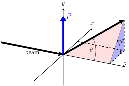
Figure 1: Definition of polar and azimuthal angles $\vartheta$ and $\varphi$ and direction of the beam polarization vector. The target is located at the origin of the coodinate system.

For this paper the most interesting variables in equation 2 are the beam polarisation $P$, describing the degree of polarization of the beam and the analyzing power $A$ describing how much the scattering process distinguishes between particles scattered to the left and right. As one can see from equation 2, one is only sensitive to the product of the analyzing power $A$ and the polarization $P$. Here we assume that the analyzing power is known and the goal is to extract from the data, i.e. the measured event kinematics, the polarization $P$, with the smallest possible statistical error.

This seems to be an easy task if all other quantities in equation 2 are known. This is often not the case. The cross section, the luminosities and the acceptance are in general not known or at least not to the required precision. Several methods to extract $P$ are discussed in the following. These methods make use of ratios where these unknown factors drop out. To simplify the discussion we consider a fixed polar angle $\vartheta$ and an acceptance constant in $\varphi$. In this case the events are distributed according to

$$\left<\frac{\mathrm{d}N(\varphi)}{\mathrm{d}\varphi}\right>=\frac{N_{0}}{2\pi}(1+AP\cos(\varphi))$$ (3)

with $N_{0}={\cal L}a\int\frac{\mathrm{d}\sigma(\vartheta)}{\mathrm{d}\Omega}\mathrm{d}\Omega={\cal L}a\sigma$. If we restrict the acceptance to the dark grey area in figure 2 the probability density function (pdf) is given by:

$$p(\varphi)=\frac{1}{4\varphi_{max}}\left(1+AP\cos(\varphi)\right)\,$$ (4)

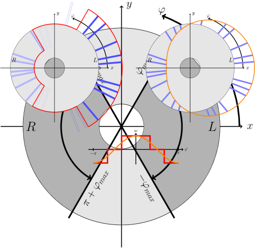
Figure 2: Events are accepted in the range $-\varphi_{max}<\varphi<\varphi_{max}$ (events scattered to the left) and $\pi+\varphi_{max}<\varphi<\pi-\varphi_{max}$ (events scattered to the right). The particle beam comes out of the plane.

3 Different ways to extract $P$

3.1 Determing $P$ using counting rates

Events are counted in the region between $-\varphi_{max}<\varphi<\varphi_{max}$ and $\pi-\varphi_{max}<\varphi<\pi+\varphi_{max}$ as indicated in figure 2. The expectation values for the number of events in the left part of the detector is given by

$$\left<N_{L}\right> = \frac{N_{0}}{2\pi}\,\int_{-\varphi_{max}}^{\varphi_{max}}\left(1+AP\cos(\varphi)\right)\mathrm{d}\varphi$$ (5)

$$= \frac{N_{0}}{2\pi}\,\left(2\varphi_{max}+AP\int_{-\varphi_{max}}^{\varphi_{max}}\cos(\varphi)\right)\mathrm{d}\varphi$$

$$= \frac{N_{0}}{\pi}\varphi_{max}\,\left(1+AP\frac{\int_{-\varphi_{max}}^{\varphi_{max}}\cos(\varphi)\mathrm{d}\varphi}{2\varphi_{max}}\right)$$

$$= \frac{N_{0}}{\pi}\varphi_{max}\,\left(1+AP\,\overline{\cos(\varphi)}\right)\,.$$

In a similar way one finds

$$\left<N_{R}\right>=\frac{N_{0}}{\pi}\varphi_{max}\,\left(1-AP\,\overline{\cos(\varphi)}\right)\,.$$ (6)

The following estimator can be used to determine $P$:

$$\hat{P}=\frac{1}{A\,\overline{\cos(\varphi)}}\,\frac{N_{L}-N_{R}}{N_{L}+N_{R}}\,.$$ (7)

$N_{L}$ and $N_{R}$ are the actual measured number of events. In this ratio $a$,$\mathcal{L}$ and $\sigma$ hidden in $N_{0}$ drop out. The average $\overline{\cos(\varphi)}$ can be evaluated directly from the data, i.e.

$$\overline{\cos(\varphi)} = \frac{\int_{-\varphi_{max}}^{\varphi_{max}}\cos(\varphi)\mathrm{d}\varphi}{2\varphi_{max}}=-\frac{\int_{\pi-\varphi_{max}}^{\pi+\varphi_{max}}\cos(\varphi)\mathrm{d}\varphi}{2\varphi_{max}}$$ (8)

$$= \frac{\sum_{L}\cos(\varphi_{i})-\sum_{R}\cos(\varphi_{i})}{N_{L}+N_{R}}\,.$$

Throughout the paper we assume that the number of events is large enough such that expectation values or averages like in equation 8 can be replaced to the corresponding sums over the event sample.

Simple Gaussian error propagation for equation 7 leads to a statistical error for $P$, assuming $PA\ll 1$,

$$\sigma^{2}_{\hat{P}}=\frac{1}{\left(A\overline{\cos(\varphi)}\right)^{2}N}\,,$$ (9)

where $N=N_{L}+N_{R}$ is the total number of events.

In this context it is convenient to define the figure of merit (FOM) as

$$\mbox{FOM}=\sigma^{-2}_{\hat{P}}=\left(A\overline{\cos(\varphi)}\right)^{2}N$$ (10)

The dashed curve in figure 3 shows the FOM as a function of $\varphi_{max}$.

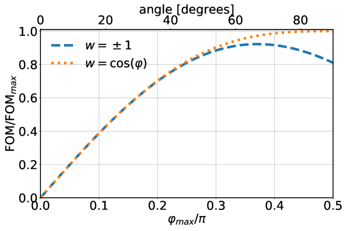
Figure 3: Figure of merit (FOM) as a function of $\varphi_{max}$ for the two weighting factors.

The curve shows an interesting behavior. Increasing $\varphi_{max}$ the FOM increases as one would expect by adding more and more events. But from 67 degrees on the FOM decreases. Thus by adding events the statistical error decreases, indicating that this is not the optimal way to analyze the data. The reason is the following. Increasing $\varphi_{max}$ one adds more data where $|\cos(\vartheta)|$ is small. Looking at equation 2 one realizes that the smaller $|\cos(\vartheta)|$ the less sensitive one is to $P$. Adding these events dilutes the sample and leads to an increase of the statistical error on $\hat{P}$. The following section discusses a more efficient way to analyze the data.

3.2 Determining $P$ using event weighting

Now we consider the following estimator

$$\hat{P}=\frac{1}{A}\,\frac{\sum_{L,R}w(\varphi_{i})}{\sum_{L,R}w(\varphi_{i})\cos(\varphi_{i})}\,.$$ (11)

Here every event is assigned a, for the moment almost arbitrary, weight factor $w(\varphi)$. The only constraint is that $w(\varphi)=-w(\varphi+\pi)$. In this case equation 11 provides an unbiased estimator for $P$. This can be verified by looking at the expectation values of the sums in equation 11:

$$AP\left<\sum_{i}w(\varphi_{i})\cos(\varphi_{i})\right> = \left<\sum w(\varphi_{i})\right>\,$$

$$APN\int_{acc}w(\varphi_{i})\cos(\varphi_{i})p(\varphi)\mathrm{d}\varphi = N\int_{acc}w(\varphi_{i})p(\varphi)\mathrm{d}\varphi\,$$

$$AP\int_{acc}w(\varphi_{i})\cos(\varphi_{i})(1+\xcancel{PA\cos(\varphi)})\mathrm{d}\varphi = \int_{acc}w(\varphi_{i})(\xcancel{1}+PA\cos(\varphi))\mathrm{d}\varphi\,.$$ (12)

Since the cosine function has the same properties as $w$, $\cos(\varphi)=-\cos(\varphi+\pi))$, the crossed out terms in equation 12 vanish, leaving on both sides $AP\int w(\varphi)\cos(\varphi)\mathrm{d}\varphi=4\varphi_{max}\overline{w\cos(\varphi)}$. Note that there is a subtle difference between average denoted as $\overline{(\dots)}$ and expectation values $\left<\dots\right>$ discussed further in appendix B.

Two cases are of interest

• simple event counting:
  $w=\begin{cases}\,\,\,1,&\text{for $-\varphi_{max}<\varphi<\varphi_{max}$}\\ -1,&\text{for $\pi-\varphi_{max}<\varphi<\pi+\varphi_{max}$}\\ \,\,\,0,&\text{otherwise}\\ \end{cases}$

• event weighting:
  $w=\begin{cases}\cos(\varphi),&\text{for $-\varphi_{max}<\varphi<\varphi_{max}$ and $\pi-\varphi_{max}<\varphi<\pi+\varphi_{max}$}\\ 0,&\text{otherwise}\\ \end{cases}$

The two cases are indicated in a pictorial way in figure 4. Note that in the case $w=\pm 1$ the estimator in equation 11 coincides with equation 7, if $\overline{\cos{\varphi}}$ is evaluated from data (see equation 8).

Figure 4: Left: event counting, Right: Weighting events with $\cos(\varphi)$. In case of event counting events are only accepted in the indicated $\varphi$ range. For the weighting method no cut is applied. The graph at the bottom shows the two weighting factors as a function of $\varphi$.

Although both cases lead to an unbiased estimator for $P$, they lead to different statistical accuracy. This will be discussed in the next subsection.

3.3 Comparison of the two weighting methods

The statistical accuracy or FOM can be obtained by simple error propagation starting from equation 11. Details of the calculations are given in appendix C. Here we just quote the result (again neglecting contributions of order $(AP)^{2}$ and higher)

$$\mbox{FOM}^{\pm 1} = NA^{2}\,\overline{\cos(\varphi)}^{2}\,,$$ (13)

$$\mbox{FOM}^{\cos(\varphi)} = NA^{2}\,\overline{\cos(\varphi)^{2}}\,.$$ (14)

The ratio of the two FOMs is

$$\frac{\overline{\cos(\varphi)^{2}}}{\left(\overline{\cos(\varphi)}\right)^{2}}\geq 1\,.$$

I.e. weighting the events with $\cos(\vartheta)$ leads in general to a higher FOM compared to the counting rate asymmetry ($w=\pm 1$). The comparison of the FOMs is shown in figure 3 by the solid and the dashed curve. At small $\varphi_{max}$ the difference between the two methods is very small. From $\varphi_{max}\approx 67$ degrees on the FOM of the counting method starts to decrease because the sample is diluted by events at small $\cos(\varphi$). Using $w=\cos(\varphi)$ the FOM still increases. This means that one can include all events without decreasing the FOM. Events at $\varphi=\pm\pi/2$ receive a weight factor 0 and are thus effectively not counted because they don’t carry any information about the polarization. This is also reflected in the fact that the dotted curve in figure 3 has slope zero at $\varphi=\pi/2$. In the counting method one should apply a cut at $\varphi_{max}\approx 67$ degrees in order to maximize the FOM. Comparing the maxima of both curves, the gain in FOM is about 8%.

In the next subsection we show that the choice $w=\cos(\varphi)$ leads to the largest reachable FOM.

3.4 Connection to Maximum Likelihood Estimator

In this subsection it is shown, that the maximum likelihood method leads to same estimator for $\hat{P}$ as the weighting method with $w=\cos(\varphi)$. Since the maximum likelihood estimator is known, at least in the large $N$ limit, to reach the minimum variance bound, this also proves that by weighting with $w=\cos(\varphi)$ one reaches the smallest statistical error or the largest FOM.

The log-likelihood function for the event distribution in equation 2 reads

$$\ell=\frac{1}{4\varphi_{max}}\,\sum_{i=1}^{N}\ln\left(1+AP\cos(\varphi)\right)\,.$$ (15)

Since the number of events $N$ is not fixed here, one should use the extended maximum likelihood method. Since $N$ does not depend on the parameter $P$ to be estimated, this is not important here.

The likelihood estimator is derived from

$$\frac{\partial\ell}{\partial P}=\sum_{i}\frac{A\cos(\varphi_{i})}{1+AP\cos(\varphi_{i})}\stackrel{{\scriptstyle!}}{{=}}0\,.$$

Assuming $AP\ll 1$, one arrives at an analytic expression

$$\hat{P}=\frac{\sum_{i}A\cos(\varphi)}{\sum_{i}(A\cos(\varphi_{i}))^{2}}=\frac{1}{A}\,\frac{\sum_{i}\cos(\varphi_{i})}{\sum_{i}\cos^{2}(\varphi_{i})}\,,$$

which is identical to the expression for $w=\cos(\varphi)$ in equation 11.

Concerning the FOM, one finds

$$\mbox{FOM}^{LH} = -\left<\frac{\partial^{2}\ell}{\partial P^{2}}\right>$$ (16)

$$= \left<\frac{A^{2}\cos(\varphi)^{2}}{(1+AP\cos(\varphi))^{2}}\right>$$

$$= \frac{N}{4\varphi_{max}}\int\frac{A^{2}\cos(\varphi)^{2}}{1+AP\cos(\varphi)}\mathrm{d}\varphi$$

$$\approx \frac{N}{4\varphi_{max}}\int A^{2}\cos(\varphi)^{2}\left(1-AP\cos(\varphi)+(AP\cos(\varphi))^{2}\right)\mathrm{d}\varphi$$

$$= NA^{2}\left(\overline{\cos(\varphi)^{2}}+(AP)^{2}\overline{\cos(\varphi)^{4}}\right)$$

$$= NA^{2}\,\overline{\cos(\varphi)^{2}}\left(1+(AP)^{2}\,\frac{\,\overline{\cos(\varphi)^{4}}\,}{\overline{\,\cos(\varphi)^{2}}\,}\right)\,,$$

which agrees with the FOM derived for $w=\cos(\varphi)$ in appendix C using error propagation, if one uses the approximation $(1+\epsilon)\approx(1-\epsilon)^{-1}$.

4 Summary and Outlook

In this note it has been shown that simply counting events is not always the best way to analyze data. One can minimize the statistical error on a polarization measurement by assigning to every event an appropriate weight factor. Concerning the statistical accuracy it was shown that a weighting factor can be found which leads to the same estimator as the maximum likelihood method, known to reach the smallest statistical error. There are cases where the likelihood may not be applied directly, e.g. when the pdf is not completely known like in case of unknown acceptance and luminosity factor. In this cases an estimator using event weighting can often still be found [4, 7].

The method can be generalized. If the detector acceptance is not restricted to one value of $\vartheta$, the analyzing power $A(\vartheta)$ can also be included in the optimal weight factor:

$$w=A(\vartheta)\cos(\varphi)\,.$$

In general, if events are distributed according to

$$p(\vec{x})\propto(1+\beta(\vec{x})P)\,$$

where $\vec{x}$ denotes a set of variables, the optimal weight factor is $w=\beta(\vec{x})$ at least for $\beta P\ll 1$. The optimal weight for the arbitrary $\beta P$ is discussed in [13].

Appendix A From event rates to cross section

This appendix shows the derivation of equation

$$N(\vartheta,\varphi)=a(\vartheta,\varphi){\cal L}\sigma(\vartheta)\left(1+PA(\vartheta)\cos(\varphi)\right)$$ (17)

The number of particles scattered to the left and right are given by

$$N(\varphi=0) = a\rho\ell\left(n^{\uparrow}\sigma_{\uparrow,L}+n^{\downarrow}\sigma_{\downarrow,L}\right)=a\rho\ell\left(n^{\uparrow}\sigma_{L}+n^{\downarrow}\sigma_{R}\right)$$ (18)

$$N(\varphi=\pi) = a\rho\ell\left(n^{\uparrow}\sigma_{\uparrow,R}+n^{\downarrow}\sigma_{\downarrow,R}\right)=a\rho\ell\left(n^{\uparrow}\sigma_{R}+n^{\downarrow}\sigma_{L}\right)$$ (19)

Here $n^{\uparrow}$ ($n^{\downarrow}$) denotes the number of beam particles with spin pointing upwards (downwards). $\rho$ is the target density and $\ell$ its length. $\sigma_{L}^{\uparrow}$ is the cross section for a beam particle with spin upwards scattered to the left. Equivalent definitions hold for the other cross sections appearing in equation 18 and 19. The second equal sign hold because of the rotational symmetry:

$$\sigma_{\downarrow,L}=\sigma_{\uparrow,R}=:\sigma_{R}\quad\mbox{and}\quad\sigma_{\downarrow,R}=\sigma_{\uparrow,L}=:\sigma_{L}$$

The beam polarization is defined as

$$P=\frac{n^{\uparrow}-n^{\downarrow}}{n^{\uparrow}+n^{\downarrow}}\,,$$ (20)

and the analyzing power is given by

$$A=\frac{\sigma_{L}-\sigma_{R}}{\sigma_{L}+\sigma_{R}}\,.$$ (21)

This allows one to write

$$N(\varphi=0) = a\rho\ell\left(n^{\uparrow}\sigma_{R}+n^{\downarrow}\sigma_{L}\right)$$

$$= a\rho l\frac{1}{2}\Big{(}n^{\uparrow}\sigma_{R}+n^{\downarrow}\sigma_{L}+n^{\uparrow}\sigma_{R}+n^{\downarrow}\sigma_{L}\Big{)}$$

$$= a\rho\ell\frac{1}{2}\Big{(}n^{\uparrow}\sigma_{R}+{n^{\uparrow}\sigma_{L}}+{n^{\downarrow}\sigma_{R}}+n^{\downarrow}\sigma_{L}$$

$$\hskip 22.76219pt+n^{\uparrow}\sigma_{R}-{n^{\uparrow}\sigma_{L}}-{n^{\downarrow}\sigma_{R}}+n^{\downarrow}\sigma_{L}\Big{)}$$

$$= a\rho\ell\frac{1}{2}\left((n^{\uparrow}+n^{\downarrow})(\sigma_{R}+\sigma_{L})+(n^{\uparrow}-n^{\downarrow})(\sigma_{R}-\sigma_{L})\right)$$

$$= a\rho\ell\underbrace{\frac{1}{2}(\sigma_{R}+\sigma_{L})}_{=\sigma}\left((n^{\uparrow}+n^{\downarrow})+(n^{\uparrow}-n^{\downarrow})\underbrace{\frac{\sigma_{R}-\sigma_{L}}{\sigma_{R}+\sigma_{L}}}_{=A}\right)$$

$$= a\rho\ell\underbrace{(n^{\uparrow}+n^{\downarrow})}_{=n}\sigma\left(1+\underbrace{\frac{n^{\uparrow}-n^{\downarrow}}{n^{\uparrow}+n^{\downarrow}}}_{=P}A\right)$$

$$= a\mathcal{L}\sigma\left(1+PA\right)\,.$$

with the luminosity $\mathcal{L}=\rho\ell n$. For the right side ($\varphi=\pi$) on finds correspondingly

$$N(\varphi=\pi) = a\mathcal{L}\sigma\left(1-PA\right)\,.$$

Again using rotational symmetry and properly normalized we find for arbitrary azimuthal angles equations 2 and  3:

$$\left<\frac{\mathrm{d}N(\varphi)}{\mathrm{d}\varphi}\right>=\frac{a\mathcal{L}\sigma}{2\pi}(1+AP\cos(\varphi))\,.$$ (22)

Appendix B Expectation values and averages

Note that there is a difference between the average denoted be $\overline{(\dots)}$ and $\left<\dots\right>$ for odd powers of the cosine function. The expectation value is defined as

$$\left<\cos(\varphi)^{2}\right> = \int_{acc}\cos(\varphi)^{2}p(\varphi)\mathrm{d}\varphi$$ (23)

$$= \frac{1}{4\varphi_{max}}\,\int_{acc}\cos(\varphi)^{2}\left(1+AP\cos(\varphi)\right)\mathrm{d}\varphi$$

$$= \frac{1}{4\varphi_{max}}\,\Big{(}\int_{-\varphi_{max}}^{\varphi_{max}}\cos(\varphi)^{2}\left(1+AP\cos(\varphi)\right)\mathrm{d}\varphi$$

$$\,\,+\int_{\pi-\varphi_{max}}^{\pi+\varphi_{max}}\cos(\varphi)^{2}\left(1+AP\cos(\varphi)\right)\mathrm{d}\varphi\,\Big{)}$$

$$= \frac{\int_{-\varphi_{max}}^{\varphi_{max}}\cos(\varphi)^{2}\mathrm{d}\varphi}{2\varphi_{max}}=\overline{\cos(\varphi)^{2}}$$

In general for even powers one obtains:

$$\left<\cos(\varphi)^{2n}\right>=\overline{\cos(\varphi)^{2n}}\,,\quad n=0,1,2,\dots\,.$$ (24)

For odd powers on the other hand we find

$$\left<\cos(\varphi)\right> = \int_{acc}\cos(\varphi)p(\varphi)\mathrm{d}\varphi$$ (25)

$$= \frac{1}{4\varphi_{max}}\,\int_{acc}\cos(\varphi)\left(1+AP\cos(\varphi)\right)\mathrm{d}\varphi$$

$$= \frac{1}{4\varphi_{max}}\,\Big{(}\int_{-\varphi_{max}}^{\varphi_{max}}\cos(\varphi)\left(1+AP\cos(\varphi)\right)\mathrm{d}\varphi$$

$$\quad\quad\,\,+\int_{\pi-\varphi_{max}}^{\pi+\varphi_{max}}\cos(\varphi)\left(1+AP\cos(\varphi)\right)\mathrm{d}\varphi\,\Big{)}$$

$$= 0+AP\left<\cos^{2}{\varphi}\right>\,.$$

In the evaluation of the FOM in equation 10 and 13

$$\overline{\cos(\varphi)}=\frac{\int_{-\varphi_{max}}^{\varphi_{max}}\cos(\varphi)\mathrm{d}\varphi}{2\varphi_{max}}=\frac{-\int_{\pi-\varphi_{max}}^{\pi+\varphi_{max}}\cos(\varphi)\mathrm{d}\varphi}{2\varphi_{max}}$$ (26)

occurred. For odd powers one obtains

$$\left<\cos(\varphi)^{2n+1}\right>=AP\left<\cos(\varphi)^{2n+2}\right>\neq\overline{\cos(\varphi)^{2n+1}}\,,\quad n=0,1,2,\dots\,.$$ (27)

Table 2 list a few expectation values and averages used in the derivations.

	$w=\pm 1$	$w=\cos(\varphi)$
$\left<w\right>$	$AP\,\overline{\cos(\varphi)}$	$AP\,\left<\cos(\varphi)^{2}\right>$
$\left<w^{2}\right>$	$1$	$\left<\cos(\varphi)^{2}\right>$
$\left<wc\right>$	$\overline{\cos(\varphi)}$	$\left<\cos(\varphi)^{2}\right>$
$\left<w^{2}c\right>$	$AP\,\left<\cos(\varphi)^{2}\right>$	$AP\,\left<\cos(\varphi)^{4}\right>$
$\left<w^{2}c^{2}\right>$	$\left<\cos(\varphi)^{2}\right>$	$\left<\cos(\varphi)^{4}\right>$

Table 2: Various expectation values for the two weighting factors.

Appendix C Error Propagation

Starting from the expression in equation 11 ($w_{i}\equiv w(\varphi_{i})$)

$$\hat{P}=\frac{1}{A}\frac{\sum_{i}w_{i}}{\sum_{i}w_{i}\cos(\varphi_{i})}\,,$$ (28)

we define

$$W = \sum_{i}w_{i}\quad\mbox{and}$$ (29)

$$V = \sum_{i}v_{i}=\sum_{i}w_{i}\cos(\varphi_{i})\,.$$ (30)

First we calculate the covariance matrix for $V$ and $W$:

$$\mbox{Cov}(W,V) = \left<WV\right>-\left<W\right>\left<V\right>$$ (31)

$$= \left<\sum_{i}w_{i}\sum_{j}v_{j}\right>-\left<\sum_{i}w_{i}\right>\left<\sum_{j}v_{j}\right>$$ (32)

$$= \left<\sum_{i=j}w_{i}v_{i}+\sum_{i\neq j}w_{i}v_{j}\right>-\left<\sum_{i}w_{i}\right>\left<\sum_{j}v_{j}\right>$$ (33)

$$= \left<N\right>\left<WV\right>+\left<N(N-1)\right>\left<W\right>\left<V\right>-\left<N\right>^{2}\left<W\right>\left<V\right>$$ (34)

$$= \left<N\right>\left<WV\right>+\left(\left<N^{2}\right>-\left<N\right>-\left<N\right>^{2}\right)\left<W\right>\left<V\right>\,.$$ (35)

Assuming a Poisson distribution for $N$, the term in parentheses vanishes. Thus the elements of the covariance matrix of $W$ and $V$ are given by:

$$\mbox{cov}(W,V) = N\left<w^{2}\cos(\varphi)\right>=\sum_{i}w_{i}^{2}\cos(\varphi_{i})\,,$$

$$\sigma_{W}^{2} = N\left<w^{2}\right>=\sum w_{i}^{2}\,,$$

$$\sigma_{V}^{2} = N\left<w^{2}\cos(\varphi)^{2}\right>=N\sum w_{i}^{2}\cos(\varphi_{i})^{2}\,.$$

Error propagation on equation 28 leads to (using the shorthand notation $c=\cos(\varphi$))

$$\sigma^{2}_{\hat{P}} = \left(\frac{\partial\hat{P}}{\partial W},\frac{\partial\hat{P}}{\partial V}\right)\left(\begin{array}[]{cc}\sigma_{W}^{2}&\mbox{cov}\\ \mbox{cov}&\sigma_{V}^{2}\end{array}\right)\left(\begin{array}[]{c}\frac{\partial\hat{P}}{\partial W}\\ \frac{\partial\hat{P}}{\partial V}\end{array}\right)$$ (40)

$$= \frac{N}{A^{2}}\left(\frac{1}{V},-\frac{W}{V^{2}}\right)\left(\begin{array}[]{cc}\left<w^{2}\right>&\left<w^{2}c\right>\\ \left<w^{2}c\right>&\left<w^{2}c^{2}\right>\\ \end{array}\right)\left(\begin{array}[]{c}\frac{1}{V}\\ -\frac{W}{V^{2}}\end{array}\right)$$ (45)

$$= \frac{1}{NA^{2}}\left(\frac{\left<w^{2}\right>}{\left<wc\right>^{2}}-2\frac{\left<w^{2}c\right>\left<w\right>}{\left<wc\right>^{3}}+\frac{\left<w^{2}c^{2}\right>\left<w\right>^{2}}{\left<wc\right>^{4}}\right)$$ (46)

In the last line we replaced $W=N\left<w\right>$ and $V=N\left<wc\right>$.

Given the properties of $w$ ($w(\varphi)=-w(\pi+\varphi))$, one finds according to table 2:

$$\left<w\right> = AP\left<wc\right>\,,$$ (47)

$$\left<w^{2}c\right> = AP\left<w^{2}c^{2}\right>\,.$$ (48)

This leads to

$$\mbox{FOM}=NA^{2}\,\frac{\left<wc\right>^{2}}{\left<w^{2}\right>}\left(1-(AP)^{2}\frac{\left<w^{2}c^{2}\right>}{\left<w^{2}\right>}\right)^{-1}\,.$$ (49)

Finally for the FOMs read

$$\mbox{FOM}^{\pm 1} = NA^{2}\,\overline{\cos(\varphi)}^{2}\left(1-(AP)^{2}\,\overline{\cos(\varphi)^{2}}\right)^{-1}\,,$$ (50)

$$\mbox{FOM}^{\cos(\varphi)} = NA^{2}\,\overline{\cos(\varphi)^{2}}\left(1-(AP)^{2}\,\frac{\overline{\cos(\varphi)^{4}}}{\overline{\cos(\varphi)^{2}}}\right)^{-1}\,.$$ (51)

To leading order equations 50 and 51 agree with the results given in equations 13 and 14. Moreover the FOM for the case $w=\cos(\varphi)$ coincides with the FOM derived for the maximum likelihood method in equation 16.

As explained in section 3.2 the estimator

$$\hat{P}=\frac{1}{\overline{\cos(\varphi)}}\frac{N_{L}-N_{R}}{N_{L}+N_{R}}$$

leads to

$$\mbox{FOM}=NA^{2}\,\overline{\cos(\varphi)}^{2}\,\left(1-(AP)^{2}\,\overline{\cos(\varphi)^{2}}\right)^{-1}\,,$$

if $\overline{\cos(\varphi)}$ is evaluated from a sum over events.

In case $\overline{\cos(\varphi)}$ is supposed to be known, e.g. from the integral $\int{\cos(\varphi)}\mathrm{d}\varphi$, the FOM is slightly different at order $(AP)^{2}$ where now a factor $\overline{\cos(\varphi)}^{2}$ instead of $\overline{\cos(\varphi)^{2}}$ appears.

$$\mbox{FOM}=NA^{2}\,\overline{\cos(\varphi)}^{2}\,\left(1-(AP)^{2}\overline{\cos(\varphi)}^{2}\right)^{-1}\,.$$

References

- [1] Pretz, J. and Müller, F., “Extraction of Azimuthal Asymmetries using Optimal Observables,” Eur. Phys. J., vol. C79, no. 1, p. 47, 2019.
- [2] B. Abi et al., “Measurement of the Positive Muon Anomalous Magnetic Moment to 0.46 ppm,” Phys. Rev. Lett., vol. 126, no. 14, p. 141801, 2021.
- [3] G. W. Bennett et al., “Statistical equations and methods applied to the precision muon (g-2) experiment at BNL,” Nucl. Instrum. Meth. A, vol. 579, pp. 1096–1116, 2007.
- [4] M. Alekseev et al., “Direct Measurement of the Gluon Polarisation in the Nucleon via Charmed Meson Production,” 2008.
- [5] J. Pretz and J.-M. Le Goff, “Simultaneous Determination of Signal and Background Asymmetries,” Nucl. Instrum. Meth., vol. A602, pp. 594–596, 2009.
- [6] J. Pretz, “Improved Method to extract Nucleon Helicity Distributions using Event Weighting,” JINST, vol. 12, no. 02, p. P02007, 2017.
- [7] F. Müller et al., “Measurement of deuteron carbon vector analyzing powers in the kinetic energy range 170-380 MeV,” Eur. Phys. J. A, vol. 56, no. 8, p. 211, 2020.
- [8] M. Diehl and O. Nachtmann, “Optimal observables for the measurement of three gauge boson couplings in e+ e- — W+ W-,” Z. Phys. C, vol. 62, pp. 397–412, 1994.
- [9] D. Atwood and A. Soni, “Analysis for magnetic moment and electric dipole moment form-factors of the top quark via ,” Phys. Rev., vol. D45, pp. 2405–2413, 1992.
- [10] W. Bernreuther, L. Chen, and O. Nachtmann, “Electric dipole moment of the tau lepton revisited,” Phys. Rev. D, vol. 103, no. 9, p. 096011, 2021.
- [11] A. Bodek, “A simple event weighting technique for optimizing the measurement of the forward-backward asymmetry of Drell-Yan dilepton pairs at hadron colliders,” Eur. Phys. J. C, vol. 67, pp. 321–334, 2010.
- [12] G. G. Ohlsen and P. W. Keaton, “Techniques for measurement of spin-1/2 and spin-1 polarization analyzing tensors,” Nucl. Instrum. Meth., vol. 109, pp. 41–59, 1973.
- [13] J. Pretz, “Comparison of methods to extract an asymmetry parameter from data,” Nucl. Instrum. Meth., vol. A659, pp. 456–461, 2011.