Solving Nonsmooth Resource Allocation Problems with Feasibility Constraints through Novel Distributed Algorithms

Abstract

The distributed non-smooth resource allocation problem over multi-agent networks is studied in this paper, where each agent is subject to globally coupled network resource constraints and local feasibility constraints described in terms of general convex sets. To solve such a problem, two classes of novel distributed continuous-time algorithms via differential inclusions and projection operators are proposed. Moreover, the convergence of the algorithms is analyzed by the Lyapunov functional theory and nonsmooth analysis. We illustrate that the first algorithm can globally converge to the exact optimum of the problem when the interaction digraph is weight-balanced and the local cost functions being strongly convex. Furthermore, the fully distributed implementation of the algorithm is studied over connected undirected graphs with strictly convex local cost functions. In addition, to improve the drawback of the first algorithm that requires initialization, we design the second algorithm which can be implemented without initialization to achieve global convergence to the optimal solution over connected undirected graphs with strongly convex cost functions. Finally, several numerical simulations verify the results.

I Introduction

As the scale of the systems in practical problems such as UAV formations [1], robotic networks [2, 3], sensor networks [4] and power systems [5, 6, 7] becomes increasingly huge, the traditional centralized algorithms to deal with optimization problems of large-scale network systems are not satisfactory. Therefore, distributed algorithms that do not require a central node and can effectively reduce communication burden, are gradually receiving attention from diverse communities.

In general, according to the optimization objective, distributed optimization problems where each agent is only allowed to exchange local information with its neighbors can be classified into the two major categories. The optimization objective of the first category is to optimize the sum of local objective functions based on the common decision variables[8, 9, 10, 11, 12]. The problem considered in this paper is the other type that requires all agents to collaboratively seek the optimum for the sum of local objective functions without consensus decision variables, nevertheless the decisions of the agents are coupled with each other owing to certain coupled constraints. Such problems are also known as resource allocation problems when the presence is coupled equality constraints, which have widespread applications in numerous different fields such as the economic dispach of smart grids and transportation networks[13, 14, 15, 16, 17, 18].

To cope with resource allocation problems with local feasible set constraints, continuous-time algorithms have been extensively investigated in recent years on account of their flexibility for application in real physical systems (see [19, 20, 21, 22, 23, 24] ). The $\epsilon$-exact penalty function is used to handle local feasible set constraints in [19]. By combining the projection operator and the primal-dual dynamics, an initialization-free distributed algorithm was designed to solve the resource allocation problem with feasible set constraints in [20]. Afterwards, based on [20], the work of [21] simplified the way of updating auxiliary variables, thereby reducing the computational complexity. An distributed algorithm is developed in [22] with the help of singular perturbation theory and certified to converge to a suboptimal allocation of the resource allocation problem under weight-balanced digraphs. In [23], in virtue of nonsmooth exact penalty functions to deal with local box constraints, a Laplace gradient dynamics-based algorithm is employed to address the economic dispatch problem. Further, the work of [24] extends the algorithm in [23] to be suitable for the agents with double-integrator dynamics and illustrates through simulation examples that there is a faster convergence rate than the case with single-integrator dynamics. It is worthwhile mentioning that the cost functions embedded in a number of engineering problems may not be differentiable (see [25, 26, 27]). Then the algorithms of the above literature (see [19, 20, 21, 22, 23, 24]) will not be applicable, since both of them assume that the cost functions are differentiable.

Up to now, there have been a few excellent results on nonsmooth resource allocation problems (see [28, 29, 30, 31, 32]). For instance, in [28, 29], distance-based exact penalty functions replace the utilization of projection operators, and an adaptive distributed algorithm is proposed for the nonsmooth resource allocation problems which have the local feasibility constraints. In addition, for the case with nonsmooth cost functions and heterogenous local constraints, a distributed algorithm is designed in [30], via differentiated projection operators, although additional computation of the tangent cone is required and the initial state is chosen to be within the local feasible set. In [31, 32], distributed algorithms are developed by virtue of projection operators and gradient descent methods for nonsmooth resource allocation problems on undirected graphs and weight-balanced digraphs, respectively.

As we all know, it is impractical in many real applications based on an undirected communication topology among agents due to physical environment constraints and their energy limitations, and it also increases the communication costs. Additionally, there will be challenges in algorithm design and convergence analysis when encountering directed topologies, and existing algorithms such as [19, 20, 21, 28, 29, 31] may not be applicable to the resource allocation problem over directed graphs. For instance, the algorithm designed in [23] can solve the case with strongly connected and weight-balanced digraphs, in which the differentiability of cost functions is indispensable.

According to the above discussions, it is evident that the nonsmooth resource allocation problem with weight-balanced digraphs and local constraints remains great research values and challenges. It is notable that the problem considered in this paper is identical to that studied in [30, 33, 32], but a novel distributed algorithm entirely different from others in the existing literature is developed. Moreover, a sufficient condition is given for the algorithm to be implemented in a fully distributed manner under undirected graphs. Compared to the existing literature, our main contributions have several aspects given as below.

1. We investigate the nonsmooth distributed resource allocation problem with heterogeneous feasible set constraints, which can be seem as an extension of the problems considered in [13, 14, 15, 16, 17, 18, 19, 20, 21, 22, 23, 24]. Unlike [19, 23, 24] where no set constraints or only box constraints are considered, the feasible set constraints here are general convex sets. Furthermore, as an improvement of [19, 20, 21, 22, 23, 24], we consider the more general case where the cost function is nonsmooth. We develop two different classes of novel algorithms based on differential inclusions and projected output feedback for the above problem and argue their convergence resorting to the nonsmooth analysis and the Lyapunov functional theory. Moreover, in contrast to [13, 14, 15, 16, 17, 18], the algorithms proposed in this article do not necessitate the communication of local gradient information, which is more effective in protecting privacy.

2. We first establish the globally asymptotic convergence for the first algorithm to the exact optimal solution under a strongly connected and weight-balanced digraph with the strong convexity assumption for local cost functions. Besides, for the case of strictly convex local costs, we characterize that the algorithm can be implemented in a fully distributed manner instead of requiring any other global information include the connectivity of the communication graph and the convexity parameters of cost functions to determine the range of the control parameters, compared to [30, 32, 33].

3. The second algorithm can be implemented in an initialization-free way under the undirected and connected graphs without satisfying certain initial conditions of decision variables as in [20, 23, 24, 28, 30] or auxiliary variables as in [19, 29, 32], which avoids the exposure of private information.

We arrange the paper in the following order. Section II gives a few useful preliminaries. Section III formulates the nonsmooth resource allocation problem. Section IV presents the main results of this paper by designing two distributed algorithms based on projected output feedback for seeking the optimum of considered problems, and providing rigorous analysis of the convergence. Section V gives numerical simulations to verify the theoretical results. Finally, section VI provides final concluding remarks.

Notations: $\mathbb{R}^{n}$ is the set of $n$-dimensional real column vectors. $1_{n}(0_{n})$ denotes the $n\times 1$ ones(zeros) vector. $I_{n}$ is the $n\times n$ identity matrix. $\otimes$ stands for the kronecker product. $col(x_{1},\ldots,x_{N})=[x_{1}^{T},\dots,x_{N}^{T}]^{T}.$ $\|A\|$ and $\|x\|$ are used to represent the spectral norm of matrix $A$ and the Euclidean norm of vector $x$, respectively. For a set $\Omega\subset\mathbb{R}^{n}$, $\partial\Omega$ and $int(\Omega)$ denote the boundary points and the relative interiors of $\Omega$, respectively. For $\Omega_{1}\subset\mathbb{R}^{n}$ and $\Omega_{2}\subset\mathbb{R}^{n}$, $\Omega_{1}\times\Omega_{2}$ is utilized to denote the cartesian product.

II Preliminaries and Formulation

II-A Graph Theory

The communication graph among $N$ agents is denoted by $\mathcal{G}=\left(\mathcal{V},\mathcal{E},\mathcal{A}\right)$, which is specified by the node set $\mathcal{V}=\{\mathcal{V}_{1},\dots,\mathcal{V}_{N}\}$ the edge set $\mathcal{E}\in\mathcal{V}\times\mathcal{V}$ and the weighted adjacency matrix $\mathcal{A}=\left(a_{ij}\right)_{N\times N}\in\mathbb{R}^{N\times N}$. If the edge $e_{ij}\in\mathcal{E}$, then $a_{ij}>0$ which indicates that node $\mathcal{V}_{i}$ can receive information from node $\mathcal{V}_{j}$; otherwise, $a_{ij}=0$. The path is described as a sequence of edges connecting a pair of distinct nodes. The undirected (directed) graph is connected (strongly connected) if any pair of nodes is linked by a path. The weighted in-degree and weighted out-degree of $\mathcal{V}_{i}$ are given by $d_{in}^{i}=\sum_{j=1}^{N}{a_{ij}}$ and $d_{out}^{i}=\sum_{j=1}^{N}{a_{ji}}$, respectively. The Laplacian matrix associated with $\mathcal{G}$ is defined as $L=D^{in}-\mathcal{A}$, where $D_{in}=\text{diag}\left\{d_{in}^{1},\dots,d_{in}^{N}\right\}\in\mathbb{R}^{N\times N}$. Evidently, $L1_{N}=0_{N}$. For a connected undirected graph, $L$ is positive semidefinite and has a simple eigenvalue $0$ with the eigenvector space $\left\{\theta\cdot 1_{N}|\theta\in\mathbb{R}\right\}$. Moreover, all eigenvalues of $L$ are nonnegative (see [34]).

Besides, we can diagonalize $L$ by orthogonal transformation, besed on the following lemma.

Lemma 1.

(see [35]) For a given connected undirected graph $\mathcal{G}_{1}$, by means of an orthogonal matrix $T=[r\;\;R]\in\mathbb{R}^{N\times N}$, we can express $L_{1}$ in the following form:

$$L_{1}=\left[\begin{matrix}r&R\\ \end{matrix}\right]\left[\begin{matrix}0&\\ &\mathcal{J}_{1}\\ \end{matrix}\right]\left[\begin{array}[]{c}r^{T}\\ R^{T}\\ \end{array}\right]$$ (3)

where $\mathcal{J}_{1}$ is a diagonal matrix composed of all positive eigenvalues of $L_{1}$, that is, $\mathcal{J}_{1}=\text{diag}\left\{\lambda_{2},\dots,\lambda_{N}\right\}$ with $0=\lambda_{1}<\lambda_{2}\leq\dots\leq\lambda_{N}$ being the positive eigenvalues of $L_{1}$. Besides, there hold $r=\frac{1}{\sqrt{N}}1_{N},\ r^{T}R=0_{N}^{T},\ R^{T}R=I_{N-1}$, and $RR^{T}=I_{N}-\frac{1}{{N}}1_{N}1_{N}^{T}$.

By utilizing $Sym(L)$ to represent $\frac{L+L^{T}}{2}$, the following statements are the equivalent representations for a weight-balaned digraph.

1. $1_{N}^{T}L=0_{N}^{T}$;

2. $Sym(L)$ is positive semidefinite;

3. $\mathcal{G}$ is weight-balanced.

Take ${\hat{\lambda}_{1}},\ldots,{\hat{\lambda}_{N}}$ with ${\hat{\lambda}_{i}}\leq{\hat{\lambda}_{j}}$ for $i\leq j$ as the other eigenvalues of $Sym(L)$. If $\mathcal{G}$ is a strongly connected digraph, then it follows that $0$ is a simple eigenvalue of $Sym(L)$ and the real part of all other eigenvalues is positive.

Lemma 2.

(see [12]) For a weight-balanced graph $\mathcal{G}_{2}$, similar to Lemma 1, with an orthogonal matrix matrix $T=[r\;\;R]\in\mathbb{R}^{N\times N}$, we can formulate $L_{2}$ as

$$L_{2}=\left[\begin{matrix}r&R\\ \end{matrix}\right]\left[\begin{matrix}0&\\ &\mathcal{J}_{2}\\ \end{matrix}\right]\left[\begin{array}[]{c}r^{T}\\ R^{T}\\ \end{array}\right]$$ (6)

where $T=\left[\begin{matrix}r&R\\ \end{matrix}\right]$ is the same as Lemma 1 and $\mathcal{J}_{2}=R^{T}L_{2}R$.

II-B Projection and Convex Analysis

In this section, we pesent some concepts and properties about the projection operater and convex analysis (see[36]). The projection operater of $p$ on a closed convex set $\Omega\subset\mathbb{R}^{n}$ is defined as $P_{\varOmega}\left(p\right)=\arg\min_{q\in\varOmega}\lVert p-q\rVert$ , where $p\in\mathbb{R}^{n}$.

Lemma 3.

For a closed covex set $\Omega\subset\mathbb{R}^{n}$, we have the following inequilities:

1. $\lVert P_{\varOmega}\left(p\right)-P_{\varOmega}\left(q\right)\rVert\leq\lVert p-q\rVert,\quad\forall p,\;q\in\mathbb{R}^{n};$

2. $\left<p-P_{\varOmega}\left(p\right),P_{\varOmega}\left(p\right)-q\right>\geq 0,\quad\forall~{}p\in\mathbb{R}^{n},~{}\forall~{}q\in\varOmega.$

Lemma 4.

For a closed convex set $\Omega\subset\mathbb{R}^{n}$, define a function on $\mathbb{R}^{n}\times\mathbb{R}^{n}$ as

$$V\left(p,q\right)=\frac{1}{2}\left(\lVert p-P_{\varOmega}\left(q\right)\rVert^{2}-\lVert p-P_{\varOmega}\left(p\right)\rVert^{2}\right).$$

We can obtain that

1. $V\left(p,q\right)\geq\frac{1}{2}\lVert P_{\varOmega}\left(p\right)-P_{\varOmega}\left(q\right)\rVert^{2};$

2. $V\left(p,q\right)$ is continuously differentiable with respect to $p$. Further, $\triangledown_{p}V\left(p,q\right)=P_{\varOmega}\left(p\right)-P_{\varOmega}\left(q\right).$

II-C Differential Inclusions and Nonsmooth Analysis

In this section, we will introduce some concepts and propositions about nonsmooth analysis and differential inclusion systems. For more details, see [37, 38].

For a locally Lipschitz function $f:\mathbb{R}^{n}\rightarrow\mathbb{R}$, the Clarke’s generalized gradient $\partial f$ is defined as

$$\partial f=co\left\{\underset{k\rightarrow+\infty}{\lim}\nabla f\left(x_{k}\right)\left|x=\underset{k\rightarrow+\infty}{\lim}x_{k},\ x_{k}\notin\mathcal{O}\cup\varOmega_{f}\right.\right\},$$

where $co\left\{\cdot\right\}$ represents convex hull, $\varOmega_{f}$ denotes the set of points in which $f$ is not diffrentiable, and $\mathcal{O}\subset\mathbb{R}^{n}$ is a set of Lebesgue measure zero. And if $f$ is convex, then the Clarke’s generalized gradient is consistent with the sub-differential. It is known that $\partial f$ takes nonempty, compact and convex values and is locally bounded and upper semicontinuous.

A differential inclusion is given by

$$\dot{x}\in\mathcal{F}(x),\quad x(0)=x_{0}$$ (7)

where $\mathcal{F}:\mathbb{R}^{n}\rightrightarrows\mathbb{R}^{n}$ represents a set-valued map. An absolutely continuous map $x:[0,~{}T]\rightarrow\mathbb{R}^{n}$ is called a Caratheodory solution of (7) on $[0,~{}T]$, if $x$ satisfies (7) for almost all $t\in\left[0,T\right]$.

Lemma 5.

If $\mathcal{F}$ is an upper semicontinuous and locally bounded set-value map, and it takes nonempty, compact, and convex values, then it can be concluded that there is a Caratheodory solution to (7) for any initial state.

The set-valued Lie derivative of a continuous differentiable function $V:\mathbb{R}^{n}\rightarrow\mathbb{R}$ along with (7) is defined as

$$\mathcal{L}_{\mathcal{F}}V=\{v^{T}\nabla V|v\in\mathcal{F}(x)\}.$$

The set-valued LaSalle invariance principle as below is essential to the subsequent proof of convergence.

Lemma 6.

Let $V:\mathbb{R}^{n}\rightarrow\mathbb{R}$ be a continuously differentiable function and $S\in\mathbb{R}^{n}$ be a compact and strongly positively invarint set for (7). Assume that the Lie derivative satisfies $\max\mathcal{L}_{\mathcal{F}}V\leq 0$ or $\mathcal{L}_{\mathcal{F}}V=\emptyset$ for all $x\in S$, and the Caratheodory solutions of (7) are bounded, then the solutions of (7) with any initial point in $S$ converges to the largest weakly positively invariant set $\mathcal{M}\subset S\cap\{x\in\mathbb{R}^{n}\,|\,0\in\mathcal{L}_{\mathcal{F}}V\left(x\right)\}$.

III Problem Formulation

The constrained resource allocation problem concerned in this article can be described as follows:

$$\min_{y\in\mathbb{R}^{Nn}} ~{}~{}f\left(y\right),\quad f\left(y\right)=\sum_{i=1}^{N}{f_{i}}\left(y_{i}\right)$$

$$\text{subject to}~{}\sum_{i=1}^{N}y_{i}=\sum_{i=1}^{N}d_{i}$$

$$y_{i}\in\Omega_{i},~{}~{}i\in\{1,\dots,N\}$$ (8)

where $y=col(y_{1},\dots,y_{N})\in\mathbb{R}^{Nn}$ consists of the local decision $y_{i}$ satisfying the local feasible set, i.e., $y_{i}\in\Omega_{i}$, and $f_{i}:\Omega_{i}\rightarrow\mathbb{R}$ is the nonsmooth local cost function. Moveover, $\sum_{i=1}^{N}y_{i}=\sum_{i=1}^{N}d_{i}$ is the network resource constraint, where $d_{i}\in\mathbb{R}^{n}$ is the local resource.

We aim to design effective distributed algorithms for the constrained problem (III) such that each agent minimizes the global cost function while sharing private information only with its neighbors.

Remark 1.

The resource allocation problem considered in this paper allows the local cost function to be non-smooth, which extends the problem considered in [19, 20, 21, 22, 23, 24]. Meanwhile, the locally feasible set is a general convex set, while only the special case of the box constraint is considered in [13, 14, 15, 16, 17, 18].

The following mild assumptions utilized in the subsequent analysis is meaningful and widely used in the literature (see [20, 30, 33, 32]).

Assumption 1.

(Slater’s condition) For each $i\in\{1,\dots,N\}$, there exists a solution $x_{i}\in int\left(\varOmega_{i}\right)$ such that $\sum_{i=1}^{N}x_{i}=\sum_{i=1}^{N}d_{i}$.

Assumption 2.

For each $i\in\{1,\dots,N\}$, $f_{i}$ is convex and locally Lipschitz continuous.

The following lemma is the optimality condition for problem (III).

Lemma 7.

(see [39, Theorem 3.34]) For each $i\in\{1,\dots,N\}$, $y_{i}^{*}\in\Omega_{i}$ is the optimal solution of (III), if and only if there exists $s\in\mathbb{R}^{n}$ such that

$$0_{Nn}\in\partial f_{i}\left(y_{i}^{\ast}\right)-s^{\ast}+N_{\varOmega_{i}}\left(y_{i}^{\ast}\right)$$ (9a)

$$\sum_{i=1}^{N}{y_{i}^{\ast}}=\sum_{i=1}^{N}{d_{i}}.$$ (9b)

Lemma 8.

For any matrix $A\in\mathbb{R}^{n\times n}$, and vector $x\in\mathbb{R}^{n}$, we have that $Ax=0_{n}$ if and only if $A^{T}Ax=0_{n}$.

Proof: If there exists $\bar{x}\in\mathbb{R}^{n}$ such that $A^{T}A\bar{x}=0_{n}$, then we can imply that $\left(A\bar{x}\right)^{T}\left(A\bar{x}\right)=\bar{x}^{T}A^{T}A\bar{x}=0$, which means that $A\bar{x}=0_{n}$.

Conversly, it is not hard to get $A^{T}A\tilde{x}=0_{n}$ from $A\tilde{x}=0_{n}$ for $\tilde{x}\in\mathbb{R}^{n}$. $\Box$

IV Main Result

In this section, two classes of algorithms are proposed to tackle the distributed resource allocation problem (III) in Section IV-A. Afterwards, the convergence properties of two algorithms are discussed in Section IV-B and Section IV-C, respectively.

IV-A Distributed Algorithm Design

In this section, we focus on the design of the distributed algorithms on the basis of projected output feedback for the problem (III).

In order to drive all agents to minimiz the global cost function while utilizing only local information, we design the distributed algorithm as follows:

$$\begin{cases}\dot{x}_{i}\in y_{i}-x_{i}-\partial f_{i}\left(y_{i}\right)+s_{i}\\ \dot{s}_{i}=k_{1}\left(w_{i}-y_{i}+d_{i}\right)+k_{2}\sum_{j=1}^{N}{a_{ij}\left(s_{j}-s_{i}\right)}\\ \dot{w}_{i}=k_{3}\sum_{j=1}^{N}{a_{ij}\left(\left(y_{j}-d_{j}+w_{j}\right)-\left(y_{i}-d_{i}+w_{i}\right)\right)}\\ y_{i}=P_{\varOmega_{i}}\left(x_{i}\right)\end{cases}$$ (10)

where

$$k_{1}>\frac{\lVert L\rVert^{2}}{\hat{\lambda}_{2}\omega},\quad k_{2}>\frac{k_{1}^{2}}{\hat{s}_{2}^{2}},\quad k_{3}>0.$$ (11)

Remark 2.

In this system, $\partial f_{i}\left(y_{i}\right)$ is utilized to seek the optimum of the nonsmooth problem (III), $s_{i}$, and $w_{i}$ are the auxiliary variables and the projected output feedback term $P_{\varOmega_{i}}\left(x_{i}\right)$ is introduced to solve the set constraints. Moreover, the projected output feedback term enable the initial state $x_{i}(0)$ to be outside of the set constraints, which is not permitted in[20, 30, 31].

For the sake of relaxing initial value demands of the algorithm (10) for auxiliary variables, we next introduce an initialization-free algorithm as follows:

$$\begin{cases}\dot{x}_{i}\in y_{i}-x_{i}-\partial f_{i}\left(y_{i}\right)+s_{i}\\ \dot{s}_{i}=k_{1}\left(w_{i}^{L}-y_{i}+d_{i}\right)+k_{2}\sum_{j=1}^{N}{a_{ij}\left(s_{j}-s_{i}\right)}\\ \dot{w}_{i}=k_{3}\sum_{j=1}^{N}{a_{ij}\left(\left(y_{j}-d_{j}+w_{j}^{L}\right)-\left(y_{i}-d_{i}+w_{i}^{L}\right)\right)}\\ y_{i}=P_{\varOmega_{i}}\left(x_{i}\right)\end{cases}$$ (12)

where $w_{i}^{L}=\sum_{j=1}^{N}{a_{ij}\left(w_{i}-w_{j}\right)}$,

$$k_{1}>\frac{\lVert L\rVert^{2}}{{\lambda}_{2}^{2}\omega},\quad k_{2}>\frac{k_{1}^{2}\lVert L\rVert^{2}}{{\lambda}_{2}^{3}},\quad k_{3}>0.$$ (13)

Remark 3.

The structure of algorithm (12) is similar to algorithm (10), the main difference being that the auxiliary variable $w_{i}^{L}$ is replaced by the $w_{i}$, which allows the algorithm to be implemented in an initialization-free manner.

Remark 4.

Notice that according to the aforesaid two algorithms (10) and (12), what information really transmitted between the agent and its neighbors is actually the overall information $y_{j}-d_{j}+w_{j}(w_{j}^{L})$ in the form of a sum, rather than the specific private information $y_{j}$, $d_{j}$, or $w_{j}(w_{j}^{L})$ alone. In this case, the agent has no way to identify specific private information from the overall information $y_{j}-d_{j}+w_{j}(w_{j}^{L})$, and the neighbor’s $y_{j}$, $d_{j}$, and $w_{j}(w_{j}^{L})$ are still unknown to the intelligence, which avoids privacy leakage in a certain sense. Moreoer, based on such a way to share sum information, it does not increase the additional communication burden of the network, campared to the current algorithms in [20, 30, 32, 33].

Remark 5.

Through the analysis in the sequel, similar to [30, 33, 40], we will see that the convergence of the algorithm requires the parameters $k_{1}$ and $k_{2}$ to meet a specific range, which depends on $\hat{\lambda}_{2},\,\lVert L\rVert\$ and $\omega$. We can pre-calculate the dependent values through an additional distributed consensus algorithm (see [41]) to determine the range of the parameters $k_{1}$ and $k_{2}$ in advance.

IV-B Convergence Analysis Of Algorithm (10)

In this section, we analyze the characteristics of the equilibrims and the convergence of (10). Specifically, the proof of the convergence is established on the nonsmooth analysis and the Lyapunov functional theory.

Let $x=col(x_{1},x_{2},\ldots,x_{N}),\;s=col(s_{1},s_{2},\ldots,s_{N}),\;w=col(w_{1},w_{2},\ldots,w_{N}),\;d=col(d_{1},d_{2},\ldots,d_{N}),\;\varOmega=\varOmega_{1}\times\varOmega_{2}\times\ldots\times\varOmega_{N},\;\partial f(y)=col(\partial f_{1}(y_{1}),\partial f_{2}(y_{2}),\ldots,\partial f_{N}(y_{N})),\;y=col(y_{1},y_{2},\ldots,y_{N})$.

We can recast (10) in a campact form as:

$$\begin{cases}\dot{x}\in y-x-\partial f\left(y\right)+s\\ \dot{s}=k_{1}\left(w-y+d\right)-k_{2}\left(L\otimes I_{n}\right)s\\ \dot{w}=-k_{3}\left(L\otimes I_{n}\right)\left(w-y+d\right)\\ y=P_{\varOmega}\left(x\right).\end{cases}$$ (14)

Natably, the existence of the solution of (14) can be guaranteed by Lemma 5 under Assumption 2.

We have the following result with regard to the equilibrium of (14).

Theorem 1.

For the nonsmooth resource allocation problem (III), consider the case where the communication topology is a strongly connected and weight-balanced digraphs. If Assumptions 1 and 2 hold, with the initial condition satisfying $\sum_{i=1}^{N}{w_{i}(0)}=0_{n}$, then $(y^{*},x^{*},s^{*},w^{*})$ is an equilibrium point of (14), if and only if $y^{*}$ is an optimal solution of (III).

Proof: 1) We assume that $(y^{*},x^{*},s^{*},w^{*})$ is an equilibrium of (14), then one has

$$0_{Nn}\in y^{\ast}-x^{\ast}-\partial f\left(y^{\ast}\right)+s^{\ast}$$ (15a)

$$0_{Nn}= k_{1}\left(w^{\ast}-y^{\ast}+d\right)-k_{2}\left(L\otimes I_{n}\right)s^{\ast}$$ (15b)

$$0_{Nn}= -k_{3}\left(L\otimes I_{n}\right)\left(w^{\ast}+y^{\ast}-d\right)$$ (15c)

$$y^{\ast}= P_{\varOmega}\left(x^{\ast}\right).$$ (15d)

Note that $L1_{N}=0_{N}$ and $1_{N}^{T}L=0_{N}^{T}$ are satisfied due to the strony connectedness and weight-balance of digraphs. Then there exists $\theta_{1}\in\mathbb{R}^{n}$ such that $\left(L\otimes I_{n}\right)s^{*}=1_{N}\otimes\theta_{1}$ form (15b) and (15c). Subsequently, one can obtain that $\left(L^{T}L\otimes I_{n}\right)s^{*}=L^{T}1_{N}\otimes\theta_{1}=0_{Nn}$, which indicates that $\left(L\otimes I_{n}\right)s^{*}=0_{Nn}$ i.e. $s_{i}^{*}=s_{j}^{*},\ \forall\ i,j\in\left\{1,\dots,N\right\}$ by Lemma 8. Further, it results from (15b) that $k_{1}\left(1_{N}^{T}\otimes I_{n}\right)\left(w^{\ast}-y^{\ast}+d\right)=k_{2}\left(1_{N}^{T}L\otimes I_{n}\right)s^{\ast}=0_{n}$. Additionally, it follows from (14) that $(1_{N}^{T}\otimes I_{n})\dot{w}(t)=0_{n},$ and applying $\sum_{i=1}^{N}{w_{i}\left(0\right)=0_{n}}$, i.e. $(1_{N}^{T}\otimes I_{n})w(0)=0_{n}$, we know that $(1_{N}^{T}\otimes I_{n}){w}\left(t\right)=0_{n}$ for any $t\geq 0$. Therefore, one can get that $k_{1}\left(1_{N}^{T}\otimes I_{n}\right)\left(-y^{*}+d\right)=0_{n}$, i.e. $\sum_{i=1}^{N}{y_{i}^{*}}=\sum_{i=1}^{N}{d_{i}}$.

Besides, from (15a) and (15d), it can be seen that $y^{\ast}=P_{\varOmega}\left(y^{\ast}-\partial f\left(y^{\ast}\right)+s^{\ast}\right)$, that is, $0_{n}\in\partial f\left(y_{i}^{*}\right)-s_{i}^{*}+N_{\varOmega_{i}}\left(y_{i}^{*}\right)$. According to the above analysis, it is concluded that $y^{*}$ is an optimal solution of the problem (III) with reference to Lemma 7.

2) If $y^{*}$ is an optimal solution of the problem (III), then there exists $s_{i}^{*}\in\mathbb{R}^{n}$, such that

$$\begin{cases}0_{n}\in\partial f_{i}\left(y_{i}^{\ast}\right)-s_{i}^{\ast}+N_{\varOmega_{i}}\left(y_{i}^{\ast}\right)\\ \sum_{i=1}^{N}{y_{i}^{\ast}}=\sum_{i=1}^{N}{d_{i}}\\ s_{i}^{\ast}=s_{j}^{\ast}\ \forall i,j\in\{1,\ldots,N\}\\ y_{i}^{\ast}\in\varOmega_{i}\ \forall i\in\{1,\ldots,N\}.\end{cases}$$ (16)

By taking $s^{*}=col\left\{s_{1}^{*},...,s_{N}^{*}\right\}$, it is obvious that $\left(L\otimes I_{n}\right)s^{*}=0_{Nn}$ based on (16).

Next, we can take $x^{*}=col\left\{x_{1}^{*},...,x_{N}^{*}\right\}$, where $x_{i}^{*}\in y_{i}^{*}-\partial f_{i}\left(y_{i}^{*}\right)+s_{i}^{*}$. Then, from (16), it follows that (15a) and (15d) hold.

Furthermore, denote $w^{*}=col\left\{w_{1}^{*},...,w_{N}^{*}\right\}$, where $w_{i}^{*}=y_{i}^{*}-d_{i}$, then (15b) and (15c) are satisfied, since $\left(L\otimes I_{n}\right)s^{*}=0_{Nn}$. Therefore, $\left(y^{*},x^{*},s^{*},w^{*}\right)$ is an equilibrium of (14). $\Box$

In the following, the asymptotic convergence associated with algorithm (10) is studied over a weight-balanced digraph and a undirected graph.

Theorem 2.

For the problem (III) with Assumptions 1 and 2, consider the case where the local cost functions are $\omega$-strongly convex and the communication topology is a strongly connected and weight-balanced digraph. Suppose that the initial point $(y(0),x(0),s(0),w(0))$ satisfies $\sum_{i=1}^{N}{w_{i}\left(0\right)=0_{n}}$, then the algorithm (10) can converge asymptotically to the optimum of problem (III).

Proof: In what follows, without loss of generality, let $n=1$ for simplicity. To prove the assertion in theorem 2, we implement the following orthogonal transformation from Lemma 1:

$$\tilde{s}= {\mathrm{col}}({\tilde{s}_{1}},{\tilde{s}_{2}})={\begin{bmatrix}r&R\end{bmatrix}^{T}}s$$ (17a)

$$\tilde{w}= {\mathrm{col}}({\tilde{w}_{1}},{\tilde{w}_{2}})={\begin{bmatrix}r&R\end{bmatrix}^{T}}w$$ (17b)

$$\tilde{s}^{*}= {\mathrm{col}}({\tilde{s}_{1}}^{*},{\tilde{s}_{2}}^{*})={\begin{bmatrix}r&R\end{bmatrix}^{T}}s^{*}$$ (17c)

$$\tilde{w}^{*}= {\mathrm{col}}({\tilde{w}_{1}}^{*},{\tilde{w}_{2}}^{*})={\begin{bmatrix}r&R\end{bmatrix}^{T}}w^{*}$$ (17d)

where $\tilde{s}_{1},\tilde{w}_{1},\tilde{s}_{1}^{*},\tilde{w}_{1}^{*}\in\mathbb{R}$ and $\tilde{s}_{2},\tilde{w}_{2},\tilde{s}_{2}^{*},\tilde{w}_{2}^{*}\in\mathbb{R}^{N-1}.$ As a consequence, one can equivalently rewrite (14) as

$$\begin{cases}\dot{x}\in y-x-\partial f\left(y\right)+\left[r\ R\right]s\\ \dot{\tilde{s}}_{1}=-k_{1}r^{T}\left(y-d\right)\\ \dot{\tilde{s}}_{2}=k_{1}\left(\tilde{w}_{2}-R^{T}\left(y-d\right)\right)-k_{2}R^{T}LR\tilde{s}_{2}\\ \dot{\tilde{w}}_{1}=0\\ \dot{\tilde{w}}_{2}=k_{3}R^{T}L\left(y-d\right)-k_{3}R^{T}LR\tilde{w}_{2}\\ y=P_{\varOmega}\left(x\right).\end{cases}$$ (18)

To proceed, we only need to analyze the convergence of (18).

Consider a Lyapunov function candidate as

$$V_{1}=~{} \frac{k_{1}}{2}\left(\lVert x-P_{\varOmega}\left(x^{*}\right)\rVert^{2}-\lVert x-P_{\varOmega}\left(x\right)\rVert^{2}\right)$$

$$+\frac{1}{2}\lVert\tilde{s}_{1}-\tilde{s}_{1}^{*}\rVert^{2}+\frac{1}{2}\lVert\tilde{s}_{2}-\tilde{s}_{2}^{*}\rVert^{2}$$

$$+\frac{1}{2k_{3}}\lVert\tilde{w}_{2}-\tilde{w}_{2}^{*}\rVert^{2}$$ (19)

where $\left(x^{*},\tilde{s}_{1}^{*},\tilde{s}_{2}^{*},\tilde{w}_{2}^{*}\right)$ is an equilibrium point of (15), and $k_{1},k_{3}$ satisfies (11) . With reference to Lemma 4, one can obtain that

$$V_{1}\geq~{} \,\frac{k_{1}}{2}\lVert y-y^{*}\rVert^{2}+\frac{1}{2}\lVert\tilde{s}_{1}-\tilde{s}_{1}^{*}\rVert^{2}$$

$$+\frac{1}{2k_{3}}\lVert\tilde{w}_{2}-\tilde{w}_{2}^{*}\rVert^{2}+\frac{1}{2}\lVert\tilde{s}_{2}-\tilde{s}_{2}^{*}\rVert^{2}.$$ (20)

The set-valued Lie derivative of $V_{1}$ along (18) is expressed as $\mathcal{L}_{\left(\ref{zal1}\right)}V_{1}$. For any $\zeta_{1}\in\mathcal{L}_{\left(\ref{zal1}\right)}V_{1}$, there exist $\gamma\in\partial f\left(y\right)$ and $\gamma^{*}\in\partial f\left(y^{*}\right)$ such that

$$\zeta_{1}=~{} k_{1}\lVert y-y^{*}\rVert^{2}-k_{1}\left(y-y^{*}\right)^{T}\left(x-x^{*}\right)$$

$$+k_{1}\left(\left[r\,\,R\right]\tilde{s}-\left[r\,\,R\right]\tilde{s}^{*}\right)^{T}\left(y-y^{*}\right)$$

$$-k_{1}\left(\gamma-\gamma^{*}\right)^{T}\left(y-y^{*}\right)$$

$$-k_{1}\left(\tilde{s}_{2}-\tilde{s}_{2}^{*}\right)^{T}R^{T}Sym\left(L\right)R\left(\tilde{s}_{2}-\tilde{s}_{2}^{*}\right)$$

$$-k_{1}\left(\tilde{s}_{2}-\tilde{s}_{2}^{*}\right)^{T}R^{T}\left(y-y^{*}\right)$$

$$+k_{1}\left(\tilde{s}_{2}-\tilde{s}_{2}^{*}\right)^{T}\left(\tilde{w}_{2}-\tilde{w}_{2}^{*}\right)$$

$$-\left(\tilde{w}_{2}-\tilde{w}_{2}^{*}\right)^{T}R^{T}L\left(y-y^{*}\right)$$

$$-\left(\tilde{w}_{2}-\tilde{w}_{2}^{*}\right)^{T}R^{T}Sym\left(L\right)R\left(\tilde{w}_{2}-\tilde{w}_{2}^{*}\right)$$

$$-k_{1}\left(\tilde{s}_{1}-\tilde{s}_{1}^{*}\right)^{T}r^{T}\left(y-y^{*}\right)$$

$$=~{} k_{1}\lVert y-y^{*}\rVert^{2}-k_{1}\left(y-y^{*}\right)^{T}\left(x-x^{*}\right)$$

$$-k_{1}\left(\gamma-\gamma^{*}\right)^{T}\left(y-y^{*}\right)$$

$$-k_{2}\left(\tilde{s}_{2}-\tilde{s}_{2}^{*}\right)^{T}R^{T}Sym\left(L\right)R\left(\tilde{s}_{2}-\tilde{s}_{2}^{*}\right)$$

$$+k_{1}\left(\tilde{s}_{2}-\tilde{s}_{2}^{*}\right)^{T}\left(\tilde{w}_{2}-\tilde{w}_{2}^{*}\right)$$

$$-\left(\tilde{w}_{2}-\tilde{w}_{2}^{*}\right)^{T}R^{T}L\left(y-y^{*}\right)$$

$$-\left(\tilde{w}_{2}-\tilde{w}_{2}^{*}\right)^{T}R^{T}Sym\left(L\right)R\left(\tilde{w}_{2}-\tilde{w}_{2}^{*}\right)$$ (21)

where the second equality follows from (17).

With reference to the property of projection given in Lemma 3 and the strongly convexity of cost function, one can obtain that

$$-\left(y-y^{*}\right)^{T}\left(x-x^{*}\right)+\lVert y-y^{*}\rVert^{2}\leq 0,$$ (22)

$$-k_{1}\left(\gamma-\gamma^{*}\right)^{T}\left(y-y^{*}\right)\leq-k_{1}\omega\lVert y-y^{*}\rVert^{2}.$$ (23)

Applying the Yong’s inequality, it yields

$$k_{1}\left(\tilde{s}_{2}-\tilde{s}_{2}^{*}\right)^{T}\left(\tilde{w}_{2}-\tilde{w}_{2}^{*}\right)\leq \frac{k_{1}^{2}}{\hat{\lambda}_{2}}\lVert s_{2}-\tilde{s}_{2}^{*}\rVert^{2}$$

$$+\frac{\hat{\lambda}_{2}}{4}\lVert w_{2}-\tilde{w}_{2}^{*}\rVert^{2},$$ (24)

$$-\left(\tilde{w}_{2}-\tilde{w}_{2}^{*}\right)^{T}R^{T}L\left(y-y^{*}\right)\leq \frac{\hat{\lambda}_{2}}{4}\lVert w_{2}-\tilde{w}_{2}^{*}\rVert^{2}$$

$$+\frac{\lVert L\rVert^{2}}{\hat{\lambda}_{2}}\lVert\left(y-y^{*}\right)\rVert^{2}.$$ (25)

Besides, equipped with the weight-balanced and strongly connected graph, it can be verified that

$$-k_{2}\left(\tilde{s}_{2}-\tilde{s}_{2}^{*}\right)^{T}R^{T}Sym\left(L\right)R\left(\tilde{s}_{2}-\tilde{s}_{2}^{*}\right)$$

$$\leq-k_{2}\hat{\lambda}_{2}\lVert s_{2}-\tilde{s}_{2}^{*}\rVert^{2},$$ (26)

$$-\left(\tilde{w}_{2}-\tilde{w}_{2}^{*}\right)^{T}R^{T}Sym\left(L\right)R\left(\tilde{w}_{2}-\tilde{w}_{2}^{*}\right)$$

$$\leq-\hat{\lambda}_{2}\lVert w_{2}-\tilde{w}_{2}^{*}\rVert^{2}.$$ (27)

Consequently, in combination with (IV-B)-(IV-B), direct calculation yields

$$\zeta_{1}\leq -\tau_{1}$$ (28)

where

$$\tau_{1}= \left(k_{1}\omega-\frac{\lVert L\rVert^{2}}{\hat{\lambda}_{2}}\right)\lVert y-y^{*}\rVert^{2}$$

$$+\left(k_{2}\hat{\lambda}_{2}-\frac{k_{1}^{2}}{\hat{\lambda}_{2}}\right)\lVert s_{2}-\tilde{s}_{2}^{*}\rVert^{2}$$

$$+\frac{\hat{\lambda}_{2}}{2}\lVert\tilde{w}_{2}-\tilde{w}_{2}^{*}\rVert^{2}\geq 0.$$ (29)

It follows from the arbitrariness of $\zeta_{1}$, that

$$\max\mathcal{L}_{(\ref{zal1})}V_{1}\leq-\tau_{1}\leq 0.$$ (30)

Combining (30) and (IV-B), one can arrive at the boundedness of $\left(y\left(t\right),\tilde{s}_{1}\left(t\right),\tilde{s}_{2}\left(t\right),\tilde{w}_{2}\left(t\right)\right)$ for any $t\geq 0$. Due to the compactness of $\partial f\left(y\right)$, there exists $M>0$ such that

$$\lVert y\left(t\right)-\gamma+\left[r\ R\right]s\left(t\right)\rVert\leq M,\forall\gamma\in\partial f\left(y\left(t\right)\right),t\geq 0.$$ (31)

In the sequel, based on the expression of $\dot{x}\left(t\right)$, we show that $x\left(t\right)$ is also bounded. Define $W\left(x\right)=\frac{1}{2}\lVert x\rVert^{2}$. One can obtain that

$$\mathcal{L}_{(\ref{zal1})}W=\left\{x^{T}\left(-x+y-\gamma-\left[r\ R\right]\tilde{s}\right):\gamma\in\ \partial f\left(y\right)\right\}.$$

Subsequently, with $M$ defined in (3), we have $\max\mathcal{L}_{(\ref{zal1})}W\left(x\left(t\right)\right)\leq-\lVert x\left(t\right)\rVert^{2}+M\lVert x\left(t\right)\rVert=-2W\left(x\left(t\right)\right)+M\sqrt{2W\left(x\left(t\right)\right)}$, which can verify the boundness of $x\left(t\right)$. To proceed, based on Lemma 6, the solution of (10) converges to the set $S$ as follows:

$$S=\big{\{}\left(x,\tilde{s}_{2},\tilde{w}_{2}\right)\in~{} \mathbb{R}^{N}\times\mathbb{R}^{N-1}\times\mathbb{R}^{N-1}:$$

$$y=y^{*},\tilde{s}_{2}=\tilde{s}_{2}^{*},\tilde{w}_{2}=\tilde{w}_{2}^{*}\big{\}}.$$

Thus, it indicates that $\lim_{t\rightarrow\infty}y\left(t\right)=y^{*}$ and the proof is completed by Theorem 1. $\Box$

Remark 6.

Theorem 2 shows the effectiveness of algorithm (10) with non-smooth resource allocation under a weight-balanced digraph. Note that the weight-balanced digraph is a more general assumption than the undirected graph, which may cause the algorithm in [31, 15, 28, 29] to not be applicable to the problem solved in Theorem 2.

Theorem 3.

For the problem (III) with Assumptions 1 and 2, consider the case where the local cost functions are strictly convex and the communication topology is a connected and undirected graph. Suppose the initial point $(y(0),x(0),s(0),w(0))$ satisfies $\sum_{i=1}^{N}{w_{i}\left(0\right)=0_{n}}$, then the algorithm (10) can converge asymptotically to the optimal solution of problem (III).

Proof: Similar to the previous proof, we assume $n=1$. Take consider of the following Lyapunov function candidate

$$V_{2}=~{} \frac{k_{1}}{2}\left(\lVert x-P_{\varOmega}\left(x^{*}\right)\rVert^{2}-\lVert x-P_{\varOmega}\left(x\right)\rVert^{2}\right)$$

$$+\frac{k_{3}}{2k_{2}}\lVert\frac{k_{1}}{k_{3}}\mathcal{J}_{1}^{-1}\left(\tilde{w}_{2}-\tilde{w}_{2}^{*}\right)+\tilde{s}_{2}-\tilde{s}_{2}^{*}\rVert^{2}$$

$$+\frac{1}{2}\lVert\tilde{s}_{1}-\tilde{s}_{1}^{*}\rVert^{2}+\frac{1}{2}\lVert\tilde{s}_{2}-\tilde{s}_{2}^{*}\rVert^{2}$$ (32)

where $\mathcal{J}_{1}$ is defined in Lemma 1, $\left(x^{*},\tilde{s}_{1}^{*},\tilde{s}_{2}^{*},\tilde{w}_{2}^{*}\right)$ is an equilibrium point of (14), and $k_{1},k_{2},k_{3}>0$. With reference to Lemma 4, one can obtain that

$$V_{2}\geq \frac{k_{1}}{2}\lVert y-y^{*}\rVert^{2}+\frac{1}{2}\lVert\tilde{s}_{1}-\tilde{s}_{1}^{*}\rVert^{2}+\frac{1}{2}\lVert\tilde{s}_{2}-\tilde{s}_{2}^{*}\rVert^{2}$$

$$+\frac{k_{3}}{2k_{2}}\lVert\frac{k_{1}}{k_{3}}\mathcal{J}^{-1}\left(\tilde{w}_{2}-\tilde{w}_{2}^{*}\right)+\tilde{s}_{2}-\tilde{s}_{2}^{*}\rVert^{2}.$$ (33)

Similarly, for any $\zeta_{2}\in\mathcal{L}_{\left(\ref{zal1})\right)}V_{2}$, there exist $\gamma\in\partial f\left(y\right)$ and $\gamma^{*}\in\partial f\left(y^{*}\right)$ such that

$$\zeta_{2}=~{} k_{1}\lVert y-y^{*}\rVert^{2}-k_{1}\left(y-y^{*}\right)^{T}\left(x-x^{*}\right)$$

$$+k_{1}\left(\left[r\,\,R\right]\tilde{s}-\left[r\,\,R\right]\tilde{s}^{*}\right)^{T}\left(y-y^{*}\right)$$

$$-k_{1}\left(\gamma-\gamma^{*}\right)^{T}\left(y-y^{*}\right)$$

$$-k_{1}\left(\tilde{s}_{1}-\tilde{s}_{1}^{*}\right)^{T}r^{T}\left(y-y^{*}\right)$$

$$-k_{1}\left(\tilde{s}_{2}-\tilde{s}_{2}^{*}\right)^{T}R^{T}\left(y-y^{*}\right)$$

$$-(k_{2}+k_{3})\left(\tilde{s}_{2}-\tilde{s}_{2}^{*}\right)^{T}R^{T}LR\left(\tilde{s}_{2}-\tilde{s}_{2}^{*}\right).$$ (34)

To proceed, it is straightforward to calculate that

$$\zeta_{2}\leq-\tau_{2}$$ (35)

where

$$\tau_{2}= \left(k_{2}+k_{3}\right)\left(\tilde{s}_{2}-\tilde{s}_{2}^{*}\right)^{T}R^{T}LR\left(\tilde{s}_{2}-\tilde{s}_{2}^{*}\right)$$

$$+\left(\gamma-\gamma^{*}\right)^{T}\left(y-y^{*}\right)\geq 0.$$ (36)

Then, form the arbitrainess of $\zeta_{2}$, it follows that $\max\mathcal{L}_{(\ref{zal1})}V_{2}\leq-\tau_{2}\leq 0.$ In a similar way to the arguments shown in the demonstration of Theorem 2, it is verified that $y\left(t\right),\tilde{s}_{1}\left(t\right),\tilde{s}_{2}\left(t\right),\tilde{w}_{2}\left(t\right)$ and $x(t)$ are bounded. Then in light of Lemma 6 the solution of (14) is convergent to the largest weakly positively invariant set contained in $Q$, where

$$Q=\big{\{}\left(x,\tilde{s},\tilde{w}_{2}\right)\in~{} \mathbb{R}^{N}\times\mathbb{R}^{N}\times\mathbb{R}^{N-1}:$$

$$\ 0\in\max\mathcal{L}_{\left(\ref{zal1}\right)}V_{2}\left(x,\tilde{s},\tilde{w}_{2}\right)\big{\}}.$$

Furthermore, because of the strict convexity of $f_{i}$, one has $\left(\gamma-\gamma^{*}\right)^{T}\left(y-y^{*}\right)>0,\ \forall\ y\neq y^{*}.$ Consequently, $\lim_{t\rightarrow\infty}y\left(t\right)=y^{*}$. $\Box$

Remark 7.

Theorem 3 shows that algorithm (10) can deal with the problem of non-smooth resource allocation on undirected connected graphs in a fully distributed manner, which means that we do not need to estimate the range of parameters $k_{1}$ and $k_{2}$ through additional calculations.

Remark 8.

It is worthwhile to point out that the selecetion of parameters is covering a wide range while it is necessary in [33] that $k_{1}=k_{2}=1$. It is indicated that we can achieve different convergence rates by choosing the appropriate parameters.

IV-C Convergence Analysis Of Algorithm (12)

In this section, the property corresponding to the equilibrium point of (12) is first decribed in Theorem 4. Then the non-smooth analysis and the Lyapunov functional theory are employed to demonstrate the convergence of (12) in Theorem 5.

Let $x=col(x_{1},x_{2},\ldots,x_{N}),\;s=col(s_{1},s_{2},\ldots,s_{N}),\;w=col(w_{1},w_{2},\ldots,w_{N}),\;d=col(d_{1},d_{2},\ldots,d_{N}),\;\varOmega=\varOmega_{1}\times\varOmega_{2}\times\ldots\times\varOmega_{N},\;\partial f(y)=col(\partial f_{1}(y_{1}),\partial f_{2}(y_{2}),\ldots,\partial f_{N}(y_{N})),\;y=col(y_{1},y_{2},\ldots,y_{N})$.

Obviously, algorithm (12) amounts to the following campact form

$$\begin{cases}\dot{x}\in y-x-\partial f\left(y\right)+s\\ \dot{s}=k_{1}\left(\left(L\otimes I_{n}\right)w-y+d\right)-k_{2}\left(L\otimes I_{n}\right)s\\ \dot{w}=-k_{3}\left(L\otimes I_{n}\right)\left(\left(L\otimes I_{n}\right)w-y+d\right)\\ y=P_{\varOmega}\left(x\right).\end{cases}$$ (37)

By virtue of Lemma 5 and Assumption 2, it is observed that the system (37) exists a solution.

The result given in the following is concerning the equilibrium point of (37).

Theorem 4.

For the nonsmooth resource allocation problem (III), consider the case where the communication topology is a connected and undirected graph. If Assumptions 1 and 2 hold, then $(y^{*},x^{*},s^{*},w^{*})$ is an equilibrium point of (37), if and only if $y^{*}$ is an optimal solution of the problem (III).

Proof: 1) Let $(y^{*},x^{*},s^{*},w^{*})$ be an equilibrium point of (37), then one has

$$0_{Nn}\in~{} y^{\ast}-x^{\ast}-\partial f\left(y^{\ast}\right)+s^{\ast}$$ (38a)

$$0_{Nn}=~{} k_{1}\left(\left(L\otimes I_{n}\right)w^{\ast}-y^{\ast}+d\right)-k_{2}\left(L\otimes I_{n}\right)s^{\ast}$$ (38b)

$$0_{Nn}=~{} -k_{3}\left(L\otimes I_{n}\right)\left(\left(L\otimes I_{n}\right)w^{\ast}-y^{\ast}+d\right)$$ (38c)

$$y^{\ast}=~{} P_{\varOmega}\left(x^{\ast}\right).$$ (38d)

Firstly, according to (38c), there exists $\theta_{2}\in\mathbb{R}^{n}$ such that $\left(L\otimes I_{n}\right)w^{\ast}-y^{\ast}+d=1_{N}\otimes\theta_{2}$ due to the connectedness of the undirected graphs. Thus, (38b) indicates that $k_{2}\left(L\otimes I_{n}\right)s^{*}=k_{1}\left(1_{N}\otimes\theta_{2}\right)$ and $k_{2}\left(L^{T}L\otimes I_{n}\right)s^{*}=k_{1}\left(L^{T}1_{N}\otimes\theta_{2}\right)=0_{Nn}$. Based on Lemma 8, it follows that $\left(L\otimes I_{n}\right)s^{\ast}=0_{Nn}$, i.e. $s_{i}^{*}=s_{j}^{*},\forall\,i,j\in\{1,\dots,N\}$.

Next, form (38b), it can be calculated that $k_{1}\left(1_{N}^{T}\otimes I_{n}\right)\left(-y^{*}+d\right)=k_{2}\left(1_{N}^{T}L\otimes I_{n}\right)s^{*}-k_{1}\left(1_{N}^{T}L\otimes I_{n}\right)w^{*}=0_{n}$, which signifies that $\sum_{i=1}^{N}{y_{i}^{*}=}\sum_{i=1}^{N}{d_{i}}$.

Finally, (38a) and (38d) imply that $y^{*}=P_{\varOmega}\left(y^{*}-\partial f\left(y^{*}\right)+s^{*}\right)$ which is identical to $0_{n}\in\partial f_{i}\left(y_{i}^{*}\right)-s_{i}^{*}+N_{\varOmega_{i}}\left(y_{i}^{*}\right)$, $\forall\in\{1,\ldots,N\}$.

Combined with the above discussions, it yields that $y^{*}$ is an optimal solution of the problem (III) by Lemma 7.

2) If $y^{*}$ is an optimal solution of the problem (III), then there exists $s_{i}^{*}\in\mathbb{R}^{n}$ satisfying (16).

Thus, we can take $s^{*}=col\left\{s_{1}^{*},\dots,s_{N}^{*}\right\}$ and claim that $\left(L\otimes I_{n}\right)s^{*}=0_{Nn}$ by (16). Based on (16), setting $x^{*}=col\left\{x_{1}^{*},\dots,x_{N}^{*}\right\}$ where $x_{i}^{*}\in y_{i}^{*}-\partial f_{i}\left(y_{i}^{*}\right)+s_{i}^{*}$, it is easy to verify that (38a) and (38b) hold.

In the sequel, we illustrate there exists $w^{*}\in\mathbb{R}^{n}$ such that $\left(L\otimes I_{n}\right)w^{*}=y^{*}-d$, which can give rise to the satisfaction of (38b) and (38c) without much effort. It follows from the connectedness of the undirected graphs that $1_{N}\otimes\xi\in ker\left(L\otimes I_{n}\right)$ for any $\xi\in\mathbb{R}^{n}$. Meanwhile, one can get $\left(y^{*}-d\right)^{T}\left(1_{N}\otimes\xi\right)=0$ due to (16). As a consequence, $y^{*}-d\in range\left(L\otimes I_{n}\right)$ by noting that $\mathbb{R}^{Nn}$ can be orthogonally decomposed by $ker\left(L\otimes I_{n}\right)$ and $range\left(L\otimes I_{n}\right)$ (see [42]). Hence, there exists $w^{*}\in\mathbb{R}^{Nn}$ such that $(L\otimes I_{n})w^{*}=y^{*}-d$.

With reference to the above analysis, it can be concluded that $\left(y^{*},x^{*},s^{*},w^{*}\right)$ is an equilibrium point of (37). $\Box$

Next, the result about the convergence of (12) over an undirected graph is presented.

Theorem 5.

For the problem (III) with Assumptions 1 and 2, consider the case where the local cost functions are $\omega$-strongly convex and the communication topology is a connected undirected graph. The algorithm (12) can converge asymptotically to the optimal solution of problem (III).

Proof: In the sequel, by assigning $n=1$, we examine the following equivalent formulation of algorithm (37) obtained by the orthogonal transformation (17):

$$\begin{cases}\dot{x}\in y-x-\partial f\left(y\right)+\left[r\ R\right]s\\ \dot{\tilde{s}}_{1}=-r^{T}\left(y-d\right)\\ \dot{\tilde{s}}_{2}=k_{1}\left(R^{T}LR\tilde{w}_{2}-R^{T}\left(y-d\right)\right)-k_{2}R^{T}LR\tilde{s}_{2}\\ \dot{\tilde{w}}_{1}=0\\ \dot{\tilde{w}}_{2}=k_{3}R^{T}L\left(y-d\right)-k_{3}R^{T}L^{2}R\tilde{w}_{2}\\ y=P_{\varOmega}\left(x\right).\end{cases}$$ (39)

Therefore, we only need to discuss the convergence of (39).

Select the Lyapunov function candidate as

$$V_{3}= \frac{k_{1}}{2}\left(\lVert x-P_{\varOmega}\left(x^{*}\right)\rVert^{2}-\lVert x-P_{\varOmega}\left(x\right)\rVert^{2}\right)$$

$$+\frac{1}{2}\lVert s_{1}-\tilde{s}_{1}^{*}\rVert^{2}+\frac{1}{2}\lVert s_{2}-\tilde{s}_{2}^{*}\rVert^{2}$$

$$+\frac{1}{2k_{3}}\lVert w_{2}-\tilde{w}_{2}^{*}\rVert^{2}$$ (40)

where $\left(x^{*},\tilde{s}_{1}^{*},\tilde{s}_{2}^{*},\tilde{w}_{2}^{*}\right)$ is an equilibrium point of (37), and $k_{1},k_{3}>0$. With reference to Lemma 4, one can obtain that

$$V_{3}\geq \frac{k_{1}}{2}\lVert y-y^{*}\rVert^{2}+\frac{1}{2}\lVert\tilde{s}_{1}-\tilde{s}_{1}^{*}\rVert^{2}$$

$$+\frac{1}{2}\lVert\tilde{s}_{2}-\tilde{s}_{2}^{*}\rVert^{2}+\frac{1}{2k_{3}}\lVert\tilde{w}_{2}-\tilde{w}_{2}^{*}\rVert^{2}.$$ (41)

Similar to the previous arguments, consider the ser-valued Lie derivative of $V_{3}$ with respect to (39). For any $\zeta_{1}\in\mathcal{L}_{\left(\ref{zal2}\right)}V_{1}$, there exist $\gamma\in\partial f\left(y\right)$ and $\gamma^{*}\in\partial f\left(y^{*}\right)$ such that

$$\zeta_{3}=~{} k_{1}\lVert y-y^{*}\rVert^{2}-k_{2}\left(y-y^{*}\right)^{T}\left(x-x^{*}\right)$$

$$+k_{1}\left(\left[r\,\,R\right]\tilde{s}-\left[r\,\,R\right]\tilde{s}^{*}\right)^{T}\left(y-y^{*}\right)$$

$$-k_{1}\left(\gamma-\gamma^{*}\right)^{T}\left(y-y^{*}\right)$$

$$-k_{2}\left(\tilde{s}_{2}-\tilde{s}_{2}^{*}\right)^{T}R^{T}LR\left(\tilde{s}_{2}-\tilde{s}_{2}^{*}\right)$$

$$-k_{1}\left(\tilde{s}_{2}-\tilde{s}_{2}^{*}\right)^{T}R^{T}\left(y-y^{*}\right)$$

$$+k_{1}\left(\tilde{s}_{2}-\tilde{s}_{2}^{*}\right)^{T}R^{T}LR\left(\tilde{w}_{2}-\tilde{w}_{2}^{*}\right)$$

$$-\left(\tilde{w}_{2}-\tilde{w}_{2}^{*}\right)^{T}R^{T}L\left(y-y^{*}\right)$$

$$-\left(\tilde{w}_{2}-\tilde{w}_{2}^{*}\right)^{T}R^{T}L^{2}R\left(\tilde{w}_{2}-\tilde{w}_{2}^{*}\right)$$

$$-k_{1}\left(\tilde{s}_{1}-\tilde{s}_{1}^{*}\right)^{T}r^{T}\left(y-y^{*}\right)$$

$$=~{} k_{1}\lVert y-y^{*}\rVert^{2}-k_{2}\left(y-y^{*}\right)^{T}\left(x-x^{*}\right)$$

$$-k_{1}\left(\gamma-\gamma^{*}\right)^{T}\left(y-y^{*}\right)$$

$$-k_{2}\left(\tilde{s}_{2}-\tilde{s}_{2}^{*}\right)^{T}R^{T}LR\left(\tilde{s}_{2}-\tilde{s}_{2}^{*}\right)$$

$$+k_{1}\left(\tilde{s}_{2}-\tilde{s}_{2}^{*}\right)^{T}R^{T}LR\left(\tilde{w}_{2}-\tilde{w}_{2}^{*}\right)$$

$$-\left(\tilde{w}_{2}-\tilde{w}_{2}^{*}\right)^{T}R^{T}L\left(y-y^{*}\right)$$

$$-\left(\tilde{w}_{2}-\tilde{w}_{2}^{*}\right)^{T}R^{T}L^{2}R\left(\tilde{w}_{2}-\tilde{w}_{2}^{*}\right).$$ (42)

According to Yong’s inequality, it implies

$$k_{1}\left(\tilde{s}_{2}-\tilde{s}_{2}^{*}\right)^{T}R^{T}LR\left(\tilde{w}_{2}-\tilde{w}_{2}^{*}\right)$$

$$\leq\frac{k_{1}^{2}\lVert L\rVert^{2}}{{\lambda}_{2}^{2}}\lVert\tilde{s}_{2}-\tilde{s}_{2}^{*}\rVert^{2}+\frac{{\lambda}_{2}^{2}}{4}\lVert\tilde{w}_{2}-\tilde{w}_{2}^{*}\rVert^{2},$$ (43a)

$$-\left(\tilde{w}_{2}-\tilde{w}_{2}^{*}\right)^{T}R^{T}L\left(y-y^{*}\right)$$

$$\leq\frac{{\lambda}_{2}^{2}}{4}\lVert\tilde{w}_{2}-\tilde{w}_{2}^{*}\rVert^{2}+\frac{\lVert L\rVert^{2}}{{\lambda}_{2}^{2}}\lVert\left(y-y^{*}\right)\rVert^{2}.$$ (43b)

Utilized the fact that the connected graph is undirected and connected, one can obtain that

$$-k_{2}\left(\tilde{s}_{2}-\tilde{s}_{2}^{*}\right)^{T}R^{T}LR\left(\tilde{s}_{2}-\tilde{s}_{2}^{*}\right) \leq-k_{2}{\lambda}_{2}\lVert\tilde{s}_{2}-\tilde{s}_{2}^{*}\rVert^{2},$$ (44a)

$$-\left(\tilde{w}_{2}-\tilde{w}_{2}^{*}\right)^{T}R^{T}L^{2}R\left(\tilde{w}_{2}-\tilde{w}_{2}^{*}\right) \leq-{\lambda}_{2}^{2}\lVert\tilde{w}_{2}-\tilde{w}_{2}^{*}\rVert^{2}.$$ (44b)

As a result, combined with (22) (23) (43) (44), $\zeta_{3}$ can be ecaluated as

$$\zeta_{3}\leq -\left(k_{1}\omega-\frac{\lVert L\rVert^{2}}{{\lambda}_{2}^{2}}\right)\lVert y-y^{*}\rVert^{2}$$

$$-\left(k_{2}{\lambda}_{2}-\frac{k_{1}^{2}\lVert L\rVert^{2}}{{\lambda}_{2}^{2}}\right)\lVert\tilde{s}_{2}-\tilde{s}_{2}^{*}\rVert^{2}$$

$$-\frac{{\lambda}_{2}^{2}}{2}\lVert\tilde{w}_{2}-\tilde{w}_{2}^{*}\rVert^{2}.$$ (45)

In view of the above inequalities (IV-C), the remainder of this proof can be derived by similar argument in the proof of Theorem 2 and, thus, can be omitted. $\Box$

Remark 9.

Summarizing the above analysis, it is obvious that the auxiliary variable $\mu_{i}$ in algorithm (10) needs to satisfy certain initial conditions, while algorithm (12) can implement by an initialization-free way. In addition, compared with algorithm (10), the dynamics of algorithm (12) are more complicated and have higher communication costs. However, some practical application scenarios are not easy to fulfill the initial conditions in algorithm (10). In this instance, it is worthwhile to sacrifice a certain communication cost to realize the algorithm without initialization.

V Numerical Example

In this section, we provide two numerical examples to illustrate the utility and preformance of the proposed algorithms.

Example 1: In this subsection, inspired by [30], we verify the effectiveness of the algorithms through an economic dispatch problem in a smart grid. Specifically, we consider a grid composed of four generators with the interaction network described by $\mathcal{G}_{1}$ or $\mathcal{G}_{2}$ shown in Fig.1. The cost function of each generator in $M\$$ takes the form of a nonsmooth quadratic function as follows:

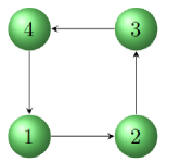
(a) $\mathcal{G}_{1}$

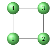
(b) $\mathcal{G}_{2}$

Figure 1: Communication graph of the network: (a) directed and weight-balanced; (b) undirected.

$$f_{i}(p_{Gi})=\alpha_{i}+\beta_{i}\|p_{Gi}-35\|+\gamma_{i}p_{Gi}^{2}$$

where $p_{Gi}$ represents the output power in $MW$ and $\alpha_{i},\beta_{i}$ and $\gamma_{i}$ denote the system parameters of generator $i$. Further, for each generator $i$, $p_{d_{i}}$ is employed to denote the local load demand.

For security, economic and other factors, in practical applications, the output power is usually specified to have a certain upper boundary $p_{Gi}^{\max}$ and a lower boundary $p_{Gi}^{\min}$, that is $p_{Gi}^{\min}\leq p_{Gi}\leq p_{Gi}^{\max}$. Specifically, for $i$th generator, the parameters in cost functions, the upper and lower bounds of output power, and the local load demand are listed in Table I.

TABLE I: Parameters setting [30]

Generator	$\alpha_{i}$	$\beta_{i}$	$\gamma_{i}$	$p_{G_{i}}^{\min}$	$p_{G_{i}}^{\max}$	$p_{d_{i}}$
$1$	$0.5$	$3$	$2$	$20$	$40$	$45$
$2$	$1.5$	$4$	$1$	$25$	$35$	$40$
$3$	$3$	$5$	$0.5$	$35$	$50$	$25$
$4$	$1$	$2$	$1.5$	$25$	$45$	$35$

By executing algorithm (10) under the weight-balanced digraph $\mathcal{G}_{1}$ shown in Fig.1(a), setting the parameters as $k_{1}=5,k_{2}=26,$ and $k_{3}=5$, and assigning auxiliary variables as $w_{i}\left(0\right)=0,i\in\{1,\ldots,4\}$, we can obtain the simulation results as depicted in Fig.3. We use dotted lines to indicate the optimal output power associated with the generator in fig.1. It can be observed from Fig.2 that the optimal value is $p_{G}^{*}=(25.8569,\,35.0000,\,50.0000,\,34.1431)^{T}$ and the output power $p_{i}$ of each generator converges to the exact optimal value. Moreover, with a simple calculation, it can be checked that the final output powers satisfy the network resource constraint.

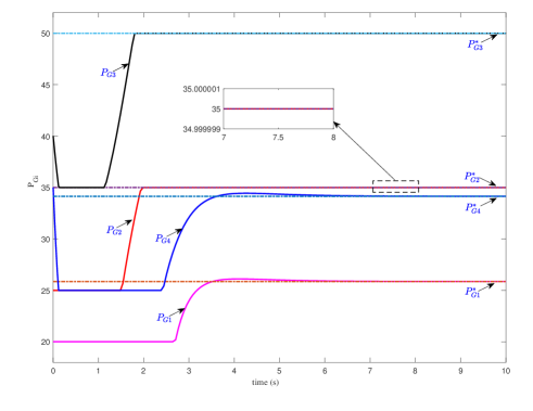
Figure 2: Simulation results of Example 1 by algorithm (10).

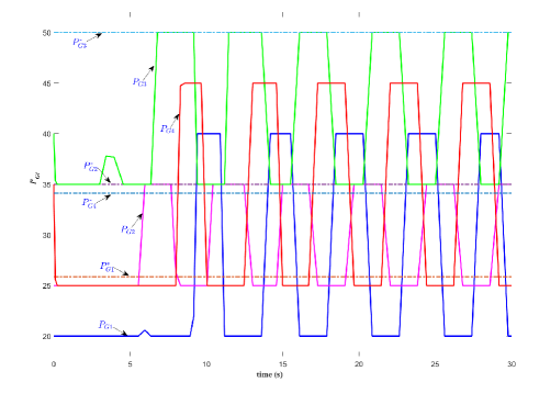
Figure 3: Simulation results of Example 1 by the algorithm proposed in [31].

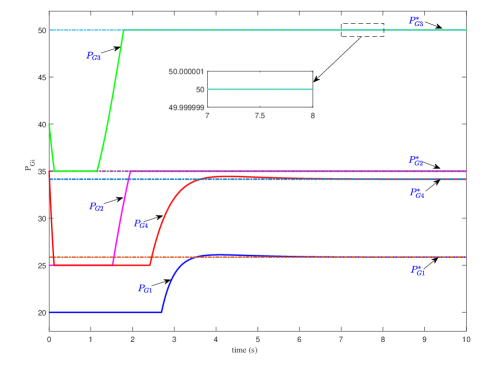
Figure 4: Simulation results of Example 1 by algorithm (12).

It is worth mentioning that, as illustrated in Fig.3, the algorithm in [31] cannot be suitable in the case that the communication network is the directed graph $\mathcal{G}_{1}$ shown in Fig.1(a). As a comparison, algorithm (10) developed in this paper overcomes the obstacles caused by a directed graph which means that it can be applied in more general practical scenarios.

Running algorithm (12) on the undirected graph $\mathcal{G}_{2}$ shown in Fig.1(b), setting the parameters to $k_{1}=5,k_{2}=55,k_{3}=5$, and configuring the auxiliary variables as $w_{i}\left(0\right)=10,i\in\{1,2,3\}$ and $w_{4}(0)=0$, we can obtain the simulation results presented in Fig.4, where the optimal output power is indicated using dotted lines. Compared to Fig.2, it is clear to observe that the output power of each generator also converges to the optimal value, even though we did not set the initial values of the auxiliary variables to satisfy specific requirements, thanks to the initialization-free nature of algorithm (12).

Example 2: Note that cost functions much more complicated than the quadratic function in Example 1 frequently appear in practical engineering. To further exemplify the generalizability of the algorithm developed in this paper, we next consider some more complex cost functions.

We consider the following problem of distributed resource allocation for four agents communicating via the two graphs shown in Fig.1, respectively.

The local cost function $f_{i}(y_{i})$, local feasible set constraint $\varOmega_{i}$, and local load demand $d_{i}$ for each agent $i\in\{1,\dots,4\},$ are defined as follows:

$$f_{1}\left(y_{1}\right)=~{} \lVert y_{1}\rVert^{2}+\lVert y_{1}-\left[2\ 2\right]^{T}\rVert$$

$$f_{2}\left(y_{2}\right)=~{} \lVert y_{2}\rVert^{2}+\frac{y_{21}^{2}}{20{y_{21}^{2}+1}}+\frac{y_{22}^{2}}{20{y_{22}^{2}+1}}$$

$$f_{3}\left(y_{3}\right)=~{} \lVert y_{3}-\left[2\ 3\right]^{T}\rVert^{2}$$

$$f_{4}\left(y_{4}\right)=~{} \ln\left(e^{-0.05y_{41}}+e^{0.05y_{41}}\right)$$

$$+\ln\left(e^{-0.05y_{42}}+e^{0.05y_{42}}\right)+\lVert y_{4}\rVert^{2}$$

$$\varOmega_{1}=~{} \left\{y_{1}\in R^{2}\left|~{}\lVert y_{1}-\left[2\ 2\right]^{T}\rVert\leq 2\right.\right\}$$

$$\varOmega_{2}=~{} \left\{y_{2}\in R^{2}\left|~{}1\leq y_{21}\leq 2,0\leq y_{22}\leq 1\right.\right\}$$

$$\varOmega_{3}=~{} \left\{y_{3}\in R^{2}\left|~{}y_{31}\geq 0.5,y_{32}\geq 1,y_{31}+y_{32}\leq 6\right.\right\}$$

$$\varOmega_{4}=~{} \left\{y_{4}\in R^{2}\left|~{}\lVert y_{4}-\left[3\ 5\right]^{T}\rVert\leq 2\right.\right\}$$

where $y_{i}=(y_{i1},y_{i2})^{T}\in\mathbb{R}^{2}$, and $d_{1}=(2,\;1)^{T}$, $d_{2}=(2,\;3)^{T}$, $d_{3}=(2,\;4)^{T}$, and $d_{3}=(1,\;5)^{T}$, respectively.

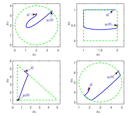
Figure 5: Evolutionary trajectories of the decisions of four agents by algorithm (10) under Fig.1(a).

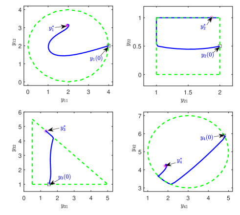
Figure 6: Evolutionary trajectories of the decisions of four agents by algorithm (10) under Fig.1(b).

Fig.5 and Fig.6 depict the simulation results of algorithm (10) under the weight-balanced digraph shown in Fig.1(a) and the undirected graph shown in Fig.1(b), respectively, where the green lines signify the local feasible set constraints and the blue lines signify the evolution of the decisions. In Fig.4, setting the parameters of algorithm (10) as $k_{1}=5,k_{2}=26$ and $k_{3}=5$, it can be noticed that the evolutionary trajectory of the decision for each agent always stays within the local feasible set and finally converges to the optimal solution.

In Fig.5, setting the parameters of algorithm 10 as $k_{1}=5,k_{2}=5$ and $k_{3}=5$, we can observe that the decisions also effectively converge to the optimal solution. In particular, in Fig.6, we set $k_{2}$ that does not satisfy the condition in (11), yet algorithm (10) is still valid, which shows that we can run algorithm (10) in a fully distributed manner under undirected graphs without additional restrictions on the parameter range, as stated in Theorem 3.

VI Conclusion

In this paper, the nonsmooth resource allocation problem with heterogeneous constraints depicted by general convex sets is investigated. We develop a novel distributed algorithm via differential inclusion and projected output feedback. It is proved that the algorithm can solve the nonsmooth resource allocation problem on weight-balanced digraphs with strongly convex cost functions. Furthermore, the algorithm is also proved to resolve the problem on undirected graphs in a fully distributed manner with strictly convex cost functions. In addition, a new algorithm is developed to improve the drawback requirement of the initialization of auxiliary variables in the first algorithm. The initialization-free algorithm is proved to address the nonsmooth resource allocation problem on undirected graphs with strongly convex cost functions by the Lyapunov functional theory and the nonsmooth analysis theory. Besides, some simulations are carried out for the effectiveness of proposed algorithms. Future work may focus on the nonsmooth resource allocation problem in the presence of communication delays or external disturbances.

References

• [1] Y. Huang, H. Wang, and P. Yao, “Energy-optimal path planning for solar-powered uav with tracking moving ground target,” Aerospace Science & Technology, vol. 53, no. Jun., pp. 241–251, 2016.
• [2] F. Bullo, J. Cortés, and S. Martínez, “Distributed control of robotic networks: A mathematical approach to motion coordination algorithms,” Princeton University Press.
• [3] Z. Feng, C. Sun, and G. Hu, “Robust connectivity preserving rendezvous of multirobot systems under unknown dynamics and disturbances,” IEEE Transactions on Control of Network Systems, vol. 4, no. 4, pp. 725–735, 2017.
• [4] C. G. Cassandras and W. Li, “Sensor networks and cooperative control,” European Journal of Control, vol. 11, no. 4, pp. 436–463, 2005.
• [5] T. Ding, R. Bo, F. Li, Y. Gu, Q. Guo, and H. Sun, “Exact penalty function based constraint relaxation method for optimal power flow considering wind generation uncertainty,” IEEE Transactions on Power Systems, vol. 30, no. 3, pp. 1546–1547, 2015.
• [6] Q. Liu, X. Le, and K. Li, “A distributed optimization algorithm based on multiagent network for economic dispatch with region partitioning,” IEEE Transactions on Cybernetics, vol. 51, no. 5, pp. 2466–2475, 2021.
• [7] K. Li, Q. Liu, S. Yang, J. Cao, and G. Lu, “Cooperative optimization of dual multiagent system for optimal resource allocation,” IEEE Transactions on Systems, Man, and Cybernetics: Systems, vol. 50, no. 11, pp. 4676–4687, 2020.
• [8] X. Zeng, P. Yi, and Y. Hong, “Distributed continuous-time algorithm for constrained convex optimizations via nonsmooth analysis approach,” IEEE Transactions on Automatic Control, vol. 62, no. 10, pp. 5227–5233, 2017.
• [9] S. Liang, X. Zeng, and Y. Hong, “Distributed nonsmooth optimization with coupled inequality constraints via modified lagrangian function,” IEEE Transactions on Automatic Control, vol. 63, no. 6, pp. 1753–1759, 2018.
• [10] Y. Wei, H. Fang, X. Zeng, J. Chen, and P. Pardalos, “A smooth double proximal primal-dual algorithm for a class of distributed nonsmooth optimization problems,” IEEE Transactions on Automatic Control, vol. 65, no. 4, pp. 1800–1806, 2020.
• [11] W. Li, X. Zeng, S. Liang, and Y. Hong, “Exponentially convergent algorithm design for constrained distributed optimization via non-smooth approach,” IEEE Transactions on Automatic Control, pp. 1–1, 2021.
• [12] S. S. K. A, J. C. b, and S. M. b, “Distributed convex optimization via continuous-time coordination algorithms with discrete-time communication,” Automatica, vol. 55, pp. 254–264, 2015.
• [13] C. Li, X. Yu, W. Yu, T. Huang, and Z. W. Liu, “Distributed event-triggered scheme for economic dispatch in smart grids,” IEEE Transactions on Industrial Informatics, vol. 12, no. 5, pp. 1775–1785, 2016.
• [14] A. Cherukuri and J. Cortes, “Distributed generator coordination for initialization and anytime optimization in economic dispatch,” Control of Network Systems IEEE Transactions on, vol. 2, no. 3, pp. 226–237, 2015.
• [15] L. Xiao and S. Boyd, “Optimal scaling of a gradient method for distributed resource allocation,” Journal Of Optimization Theory And Applications, vol. 129, no. 3, pp. 469–488, Jun. 2006.
• [16] A. Cherukuri and J. Cortés, “Initialization-free distributed coordination for economic dispatch under varying loads and generator commitment,” Automatica, vol. 74, pp. 183–193, 2016.
• [17] C. Li, X. Yu, T. Huang, and H. Xing, “Distributed optimal consensus over resource allocation network and its application to dynamical economic dispatch,” IEEE Transactions on Neural Networks and Learning Systems, vol. PP, no. 99, pp. 1–12, 2018.
• [18] W. Yu, C. Li, X. Yu, G. Wen, and J. Lü, “Economic power dispatch in smart grids: a framework for distributed optimization and consensus dynamics,” ence China Information ences, vol. 61, no. 1, pp. 1–16, 2018.
• [19] Kia and S. Solmaz, “Distributed optimal resource allocation over networked systems and use of an $\epsilon$-exact penalty function,” Ifac Papersonline, vol. 49, no. 4, pp. 13–18, 2016.
• [20] P. Yi, Y. Hong, and F. Liu, “Initialization-free distributed algorithms for optimal resource allocation with feasibility constraints and application to economic dispatch of power systems,” Automatica, vol. 74, pp. 259–269, 2016.
• [21] R. Li, “Distributed algorithm design for optimal resource allocation problems via incremental passivity theory,” Systems & Control Letters, vol. 138, 2020.
• [22] S. Liang, X. Zeng, G. Chen, and Y. Hong, “Distributed sub-optimal resource allocation via a projected form of singular perturbation,” Automatica, vol. 121, 2020.
• [23] A. Cherukuri and J. Cortés, “Distributed generator coordination for initialization and anytime optimization in economic dispatch,” IEEE Transactions on Control of Network Systems, vol. 2, no. 3, pp. 226–237, 2015.
• [24] X. He, D. W. C. Ho, T. Huang, J. Yu, H. Abu-Rub, and C. Li, “Second-order continuous-time algorithms for economic power dispatch in smart grids,” IEEE Transactions on Systems, Man, and Cybernetics: Systems, vol. 48, no. 9, pp. 1482–1492, 2018.
• [25] J.-B. Park, K.-S. Lee, J.-R. Shin, and K. Lee, “A particle swarm optimization for economic dispatch with nonsmooth cost functions,” IEEE Transactions on Power Systems, vol. 20, no. 1, pp. 34–42, 2005.
• [26] H.-T. Yang, P.-C. Yang, and C.-L. Huang, “Evolutionary programming based economic dispatch for units with non-smooth fuel cost functions,” IEEE Transactions on Power Systems, vol. 11, no. 1, pp. 112–118, 1996.
• [27] B. Fortz, L. Gouveia, and M. Joyce-Moniz, “Models for the piecewise linear unsplittable multicommodity flow problems,” European Journal of Operational Research, vol. 261, no. 1, pp. 30–42, 2017.
• [28] M. Lian, Z. Guo, X. Wang, S. Wen, and T. Huang, “Adaptive exact penalty design for optimal resource allocation,” IEEE Transactions on Neural Networks and Learning Systems, pp. 1–9, 2021.
• [29] Z. Guo, M. Lian, S. Wen, and T. Huang, “An adaptive multi-agent system with duplex control laws for distributed resource allocation,” IEEE Transactions on Network Science and Engineering, pp. 1–1, 2021.
• [30] Z. Deng, S. Liang, and Y. Hong, “Distributed continuous-time algorithms for resource allocation problems over weight-balanced digraphs,” IEEE Trans Cybern, vol. 48, no. 11, pp. 3116–3125, 2018.
• [31] X. Zeng, P. Yi, Y. Hong, and L. Xie, “Continuous-time distributed algorithms for extended monotropic optimization problems,” SIAM Journal on Control and Optimization, 2016.
• [32] Y. Zhu, W. Ren, W. Yu, and G. Wen, “Distributed resource allocation over directed graphs via continuous-time algorithms,” IEEE Transactions on Systems, Man, and Cybernetics: Systems, vol. 51, no. 2, pp. 1097–1106, 2021.
• [33] Z. Deng, X. Nian, and C. Hu, “Distributed algorithm design for nonsmooth resource allocation problems,” IEEE Trans Cybern, vol. 50, no. 7, pp. 3208–3217, 2020.
• [34] C. D. Godsil and G. Royle, Algebraic Graph Theory.   New York: Springer, 2001.
• [35] S. Yang, J. Wang, and Q. Liu, “Consensus of heterogeneous nonlinear multiagent systems with duplex control laws,” IEEE Transactions on Automatic Control, vol. 64, no. 12, pp. 5140–5147, 2019.
• [36] R. T. Rockafellar, Convex Analysis.   Princeton, N.J.: Princeton University Press, 1970.
• [37] J. P. Aubin and A. Cellina, Differential Inclusions.   Berlin Heidelberg: Springer-Verlag, 1984.
• [38] J. Cortés, “Discontinuous dynamical systems - a tutorial on solutions, nonsmooth analysis, and stability,” IEEE Control Systems Magazine, vol. 28, no. 3, pp. 36–73, Jun. 2008.
• [39] A. P. Ruszczyński, Nonlinear Optimization.   Princeton, N.J.: Princeton University Press, 2006.
• [40] Y. Zhu, G. Wen, W. Yu, and X. Yu, “Nonsmooth resource allocation of multiagent systems with disturbances: A proximal approach,” IEEE Transactions on Control of Network Systems, vol. 8, no. 3, pp. 1454–1464, 2021.
• [41] T. Charalambous, M. G. Rabbat, M. Johansson, and C. N. Hadjicostis, “Distributed finite-time computation of digraph parameters: Left-eigenvector, out-degree and spectrum,” IEEE Transactions on Control of Network Systems, vol. 3, no. 2, pp. 137–148, 2016.
• [42] G. Strang, “The fundamental theorem of linear algebra,” The American Mathematical Monthly, vol. 100, no. 9, pp. 848–855, 1993.