Multi-Agent Task Assignment in Vehicular Edge Computing: A Regret-Matching Learning-Based Approach
Abstract
Vehicular edge computing has recently been proposed to support computation-intensive applications in Intelligent Transportation Systems (ITS) such as self-driving cars and augmented reality. Despite progress in this area, significant challenges remain to efficiently allocate limited computation resources to a range of time-critical ITS tasks. To this end, the current paper develops a new task assignment scheme for vehicles in a highway. Because of the high speed of vehicles and the limited communication range of road side units (RSUs), the computation tasks of participating vehicles are to be dynamically migrated across multiple servers. We formulate a binary nonlinear programming (BNLP) problem of assigning computation tasks from vehicles to RSUs and a macrocell base station. To deal with the potentially large size of the formulated optimization problem, we develop a distributed multi-agent regret-matching learning algorithm. Based on the regret minimization principle, the proposed algorithm employs a forgetting method that allows the learning process to quickly adapt to and effectively handle the high mobility feature of vehicle networks. We theoretically prove that it converges to the correlated equilibrium solutions of the considered BNLP problem. Simulation results with practical parameter settings show that the proposed algorithm offers the lowest total delay and cost of processing tasks, as well as utility fairness among agents. Importantly, our algorithm converges much faster than existing methods as the problem size grows, demonstrating its clear advantage in large-scale vehicular networks.
Index Terms:
Correlated equilibrium, intelligent transportation systems, multi-agent learning, regret matching, task assignment, vehicular edge computingI Introduction
Due to limited computation and storage capabilities of vehicular users, it is rather difficult to meet the strict requirements of Intelligent Transportation System (ITS) applications, i.e., intensive computation and content caching with low latency [1, 2]. To this end, Vehicular Edge Computing (VEC), as an application of Mobile Edge Computing (MEC) in high-mobility environments, has been proposed as a solution [3, 4, 5, 6]. Even so, there remains the significant challenge to efficiently allocate the limited communication and computation resources of servers in VEC, due to an increasing number of vehicles that need their tasks processed.
We consider network scenarios as depicted in Fig. 1. Specifically, autonomous vehicles left-drive in two directions along a six-lane highway, similar to M Pacific Highway linking Newcastle with Sydney in New South Wales, Australia [7]. A macrocell base station (BS) is deployed to provide network connectivity along the highway. For data and computation offloading, a set of road side units (RSUs) are deployed at an inter-RSU distance of to bring the network closer to the vehicles. We denote by the set containing only the BS, and by the number of RSUs. The BS and RSUs are connected via wired links for load balancing and control coordination. Each of them is equipped with a server comprising a data processing unit and a cache.
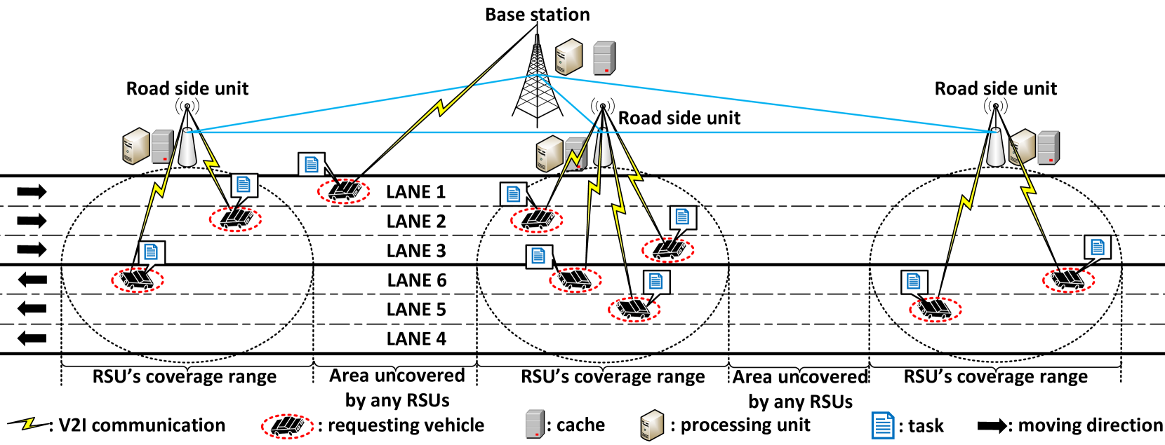
Let us assume that the vehicles have to complete computation-intensive tasks. Due to their limited computing resources, it is sensible to offload these tasks to the servers at the BS and/or the RSUs. The offload requests are sent via vehicle-to-infrastructure (V2I) communication, which is supported by the Long-Term Evolution-Advanced (LTE-A) protocol. We denote by the set of requesting vehicles, and assume a vehicle only requests to offload one task at a time. As such, we refer to vehicle and task interchangeably. Also, the number of tasks to be offloaded is equal to the number of requesting vehicles.
If a vehicle traveling at a constant speed of is still within the coverage range of an RSU , its offload request is sent directly to the RSU ; otherwise, to the BS. In either case, the server at the BS collects from all the RSUs information about task sizes, server computing capabilities, and current location and speed of vehicles. It then computes and makes a task assignment decision as to where the tasks are to be processed, i.e., at the BS or the RSUs; and in the latter case, which RSU in .
I-A Background
To address the issue of inadequate provisioning of computation resources for multiple users, [8] proposes an algorithm that optimally distributes tasks from smart mobile devices (SMDs) to MEC servers. By using a combination of particle swarm optimization, simulated annealing and genetic algorithms, this approach minimizes the energy consumed by SMDs and servers while also optimizing the task offloading ratio. In a related work by [9], tasks sent from the computers and iPads in the terminal layer are allocated to servers in the edge computing layer and cloud data layer. In order to maximize the total network profit (which is the net revenue discounted by a cost), the authors propose a task allocation strategy that utilises a swarm intelligence approach based on simulated annealing. However, without taking the mobility of SMD users into account in the problem formulation, these two algorithms are only applicable to static environments, rather than high-mobility environments (i.e. in ITS or vehicular networks).
Unlike [8, 9], the work of [10] develops a task assignment algorithm where tasks requested by vehicles are assigned to either VEC servers or volunteer vehicles in a vehicular network. The developed algorithm is based on a Stackelberg game where VEC servers and requesting vehicles are respectively modelled as leaders and followers. To completely process all the tasks, the servers recruit more volunteers while setting and sending prices to the requesting vehicles. The game strategy is to 1) maximize the income of VEC servers and volunteer vehicles, 2) reduce the cost incurred to the servers and volunteers, and 3) minimize the payment made by the requesting vehicles for processing their tasks. However, when the requesting vehicles and volunteer vehicles move in different directions and at different speeds, their connection time is limited to a brief amount due to the short communication range of vehicles (about 300 m). As a result, the requesting vehicles will be out-of-range of the volunteer vehicles, while the latter have not completely processed the tasks requested by the former.
The optimization methods for resource allocation in [8, 9, 11, 12, 10] require accurate knowledge of channel conditions which are typically time-varying and, oftentimes, unavailable in high-mobility scenarios. These solutions are typically based on a snapshot model of the vehicular networks, while ignoring the long-term influence of the current decision [3]. By contrast, without any prior knowledge of the operating environment, reinforcement learning (RL) is able to make decisions that maximize the long-term rewards for the networks according to [13] and [14]. It is arguably a promising tool to tackle problems encountered in task offloading, and communication and computation resource allocation in VEC-based ITS with time varying and unknown channel conditions.
In [15], multiple in-car applications employ an RL-based scheduling strategy to offload their tasks to MEC servers located within road side units (RSUs). Here, the latency and energy consumption for task processing are minimized. Taking a step further, a joint management scheme of spectrum, computing and storing resources in VEC is proposed in [16] using deep reinforcement learning (DRL). Note that in [15] and [16], vehicles potentially reside within the coverage range of RSUs for a short time duration only, due to their high mobility and the limited communication range of the serving RSUs (about 600 m); hence, it is possible that a vehicle moves out of the range of its serving RSU even before that RSU processes its tasks completely.
The above issue can be overcome by allowing the vehicle to migrate its tasks to the MEC servers of the next RSUs that the vehicle is about to move into. For example, in [17], there is an autonomous vehicle moving along a highway or a city expressway, and its tasks are migrated between MEC servers and processed. Assuming these MEC servers have large computation resources, [17] use DRL to minimize the energy consumption for task processing while meeting latency requirements. In addition, only a single agent interacts with the environment to determine an optimal task migration policy. Also based on DRL, [18] not only develop a task migration scheme but also find the best migration routes for vehicles in urban areas. Here, a vehicle only migrates its tasks to an MEC server if the time it takes that vehicle to reach such a server is the shortest. Compared to [17], the work of [18] could be applicable to multi-agent systems owing to utilizing communication and cooperation between multiple autonomous vehicles. However, this scheme might cause a change in the original route of vehicles as the tasks are not migrated with respect to the vehicles’ mobility pattern.
A major issue with the DRL approaches in [17] and [18] is that a significant training time is required in large environments, e.g. or more vehicles/agents, and the algorithm’s convergence is not guaranteed. To address this issue, [19] and [20] employ regret matching (RM) learning to design algorithms for multi-agent systems. The advantages of RM learning-based algorithms in several applications, e.g. seasonal forecasting and learning in matching markets without incentives, have been demonstrated by [21, 22, 23, 24]. In particular, these algorithms can converge to correlated-equilibrium solutions faster than RL-based algorithms as shown in [25] and [26]. Additionally, it is unnecessary that the correlated equilibrium solutions must be the optimal solution. Their algorithms, however, are not specifically designed for task migration in VEC, and their solutions may be rendered inapplicable due to the inherited characteristics of vehicle networks with high mobility.
I-B Contributions
In this paper, we propose a RM learning-based task assignment scheme that minimizes the total delay and cost incurred by vehicles in a highway scenario like [17]. We assume that once a vehicle leaves the coverage area of its serving RSU, it will migrate its tasks to other suitable RSUs or a macrocell base station according to its mobility pattern. The contributions of this paper are summarized as follows.
-
1.
To improve over [15] and [16], we formulate a task assignment problem as a binary nonlinear programming (BNLP) problem with specific constraints on the movement of participating vehicles. Compared to [17] and [18], this problem is formulated for migrating the tasks of multiple autonomous vehicles between servers according to these vehicles’ movement.
-
2.
Unlike [17] and [18], we reformulate the BNLP problem as a standard repeated game. Then, we propose a distributed RM algorithm that decomposes the state observations and actions of a monolithic centralized agent into those of multiple agents. In particular, this iterative game-based learning algorithm is able to guarantee an equilibrium solution. We further propose a forgetting method to speed up the convergence of the traditional RM algorithms in [19, 20]. Doing so allows the algorithm to effectively handle the high level of user mobility in vehicle networks.
-
3.
Our simulation results with practical parameter settings demonstrate the advantages of our solution in terms of delay and cost minimization, utility fairness among agents, and convergence speed particularly in large-scale network settings.
The remainder of the paper is organized as follows. Section II presents the system model, including a wireless communication model and a computation model, while Section III describes the problem formulation for task assignment. Then, Section IV proposes an RM-based solution to the task assignment problem. Here, the problem is reformulated as a repeated game while the definition of a correlated equilibrium is introduced. Section V conducts simulations to illustrate the efficiency of the proposed approach. Finally, we summarize the paper in Section VI.
II System Model
In our scenarios, once a requesting vehicle wants its task to be processed by a server at an RSU or a BS, it must send the task to the RSU/BS via a wireless link. In addition, the task can be migrated from the RSU/BS to the others via a wired connection. Thus, we first model wireless communication between the requesting vehicles and the RSUs/BS in Section II-A. Then, to determine the amount of time and cost needed for 1) uploading tasks through wireless links, 2) migrating tasks between RSUs/BS through wired links, and 3) processing tasks completely, we develop a computation model in Section II-B. The delay and cost will be used for our problem formulation in Section III.
II-A Communication Model
We consider that the received signal strength at the RSUs and BS depends only on the positional shift of the vehicles, where the effect of small-scale fading is averaged out. For interference cancellation, we adopt the orthogonal frequency-division multiplexing (OFDM) to assign orthogonal frequencies to the link between an RSU/BS and a vehicle . The data rate at which the tasks of the vehicle are uploaded to the RSU/BS at a given time is expressed as:
| (1) |
where is the link’s bandwidth, is the transmit power of the vehicle , is the link gain between the vehicle and the RSU/BS , and is the received noise power. Here, with a path-loss function, and the Euclidean distance between the vehicle and the RSU/BS at the time .
II-B Computation Model
The amount of time needed for a task to be uploaded to an RSU/BS is given by:
| (2) |
where is the size of the task .
We use two binary variables and to decide where the task is executed at the time . If the task is to be processed at an RSU/BS , then ; otherwise, . If the task is migrated and processed at the other RSU/BS , then ; otherwise, . The task migration time is calculated as [18]:
| (3) |
where is the bandwidth of the wired link between and , is the coefficient of migration delay, and is the number of hops between and .
The processing delay for the task is calculated as:
| (4) |
where is the number of CPU cycles required to completely process the task , and and cycles/s are respectively the computation capacity allocated to the task by and .
Similar to (5), the cost for processing task is given by:
| (6) |
where (t), and are respectively the costs of task uploading, task migrating and task processing.
Specifically,
| (7) |
where is the communication cost.
After the task is uploaded to , a service entity hosted at will handle the task . This entity is migrated from to if the task is not completely processed before the vehicle leaves the coverage area of . To migrate the service entity from to , the vehicle incurs the following cost [18]:
| (8) |
where is the migration cost and is the data size of each service entity.
The computation cost for the task at either RSU/BS or is expressed as:
| (9) |
where and are the unit computation costs.
III Problem Formulation
There are three constraints that describe the dependence of task assignment on the vehicle mobility, different from [18]. When a task is completely executed by an RSU , the delay for completing the task must not be larger than the duration that the vehicle resides within ’s coverage area. As such,
| (10) |
where is the distance that the vehicle travels before leaving the coverage area of .
If the task is migrated from the RSU to another RSU , the delay is instead constrained by:
| (11) |
If the task is migrated from the BS to an RSU , the delay is then constrained by:
| (12) | ||||
where is the distance that the vehicle has traveled in the area uncovered by any RSUs before it enters the coverage area of the closest RSU , and is the communication range of an RSU.
We aim to minimize the total delay and cost for completing all tasks. The task assignment in vehicular edge computing is thus formulated as the following BNLP problem.
| (13a) | ||||
| s.t. | (13b) | |||
| (13c) | ||||
| (13d) | ||||
| (13e) | ||||
| (13f) | ||||
| (13g) | ||||
where and are the weights to prioritize the delay and the cost, respectively. Constraints (13c), (13d) and (13e) show that the computation capacity assigned to a task is upper-bounded by the maximum computation capacities or . Constraint (13f) enforces that an arbitrary task must be processed by one of the RSUs and the BS.
IV Proposed Multi-Agent Regret-Matching Learning based Task Assignment Scheme
The optimization problem in (13) is nonconvex and combinatorial with nonlinear constraints. Traditional optimization methods may not be able to return a solution within an acceptable time frame, which is an important requirement in vehicular networks with a high degree of mobility. As such, we propose an iterative game-based learning algorithm that guarantees an equilibrium solution. The proposed algorithm is based on the regret minimization procedure [27, 28]. This procedure is well-known for its low complexity and provable convergence when making decisions in a situation involving multiple stakeholders.
In this paper, we consider that all tasks are homogeneous (see Section I), and the number of tasks is predefined (see Section III). The proposed solution is readily applicable to scenarios where tasks have different deadlines or different sizes, or the number of tasks varies over time. We further introduce a forgetting factor in the learning algorithm to enable fast convergence—an essential requirement in a fast-changing environment due to highly-mobile learning agents (i.e., vehicles). Using simulations with realistic network settings, we will later show that our solution adapts and converges much faster than existing approaches, especially as the number of participating vehicles (i.e., tasks) increases.
IV-A Game Reformulation for Task Assignment
We propose to reformulate problem (13) as a multi-agent distributed learning problem. Here, each requesting vehicle is an independent decision maker who learns to jointly reach an optimal solution. To ensure convergence of the learning solution at the optimum point for all the requesting vehicles, we designate the BS as a central operator. After all the requesting vehicles have played their respective actions, the operator updates each vehicle with the actions chosen by the others.
Specifically, we model the task assignment in vehicular edge computing (13) as a repeated game , where the players aim to minimize the long-run average delay and the cost to process the tasks presented by the requesting vehicles. In this model, the (finite) set of requesting vehicles is regarded as the set of players. Each player has its set of finite actions as it decides where to offload its task to. We denote by the set of joint actions of all players. Let denote the set of utility functions of all the players.
To minimize the delay and cost for processing the tasks for the vehicles, the utility function of a player at a time resulting from a given action is designed as:
| (14) |
where denotes the vector of RSU/BS actions decided by all the other players at the time . Here, if action of player satisfies all constraints in problem (13), we calculate the parameters and using (5) and (6), respectively. Otherwise, and where stands for a large positive value pre-assigned. Under this utility model, each player obtains a player-specific payoff depending on the joint action profile over all players. Here, maximizing the sum of all the players’ utilities would result in minimizing the objective function in problem (13).
IV-B Definition of Correlated Equilibrium
In most cases, a game-based solution guarantees convergence to a set of equilibria, in which any vehicle does not achieve any gain by unilaterally changing their decision. It can be shown that the equilibrium of the reformulated game is a correlated equilibrium (CE) [29, 30]. A probability distribution defined on is said to be a CE if for all player , for all and for every pair of action , it holds true that
| (15) |
When in a CE, each player does not benefit from choosing any other probability distribution over its actions, provided that all the other players do likewise.
IV-C RM-based Learning with a Forgetting Factor
An iterative algorithm that can be used to reach the CE set is the regret matching procedure proposed in [28]. The key idea is to adjust the player’s action probability to be proportional to the “regrets” for not having played other actions. Specifically, for any two actions at any time , the cumulative regret of a player up to the time for not playing action instead of its actually played action is
where denotes the indicator function. This is the change in the average payoff that the player would have if choosing a different action every time they played in the past, given that all other players did not change their decisions. A positive value indicates a “regret” by the player for not having played action instead of the chosen action .
The regret can be recursively expressed as:
| (16) |
where denotes the instantaneous regret by the player for not playing the action instead of its played action at the time . Equation (16) updates the cumulative regret at each time step by adding a correction term based on the new instantaneous regret. As a stochastic approximation method, (16), although resulting in almost surely convergence, can be quite slow. This is especially true in a dynamic environment, where player’s utility changes with time. This is likely to become a major issue in our considered vehicular networking scenario with a high degree of mobility.

| ES | TRM | RLNF | Algorithm 1 | ||
| Scenario | Forgetting factor () | N/A | N/A | N/A | |
| Minimum sum of delay and cost | |||||
| Computation time (s) | |||||
| Scenario | Forgetting factor () | N/A | N/A | N/A | |
| Minimum sum of delay and cost | N/A | ||||
| Computation time (s) | N/A |
To this end, we will now introduce a forgetting factor for updating as:
| (17) |
where is a forgetting factor used to regulate the influence of outdated values of regret over the instantaneous regret. Each player then independently chooses its next action according to the following probabilities:111 for a real number .
| (18) |
for all , and is chosen such that the probability of playing the same action in the next iteration is positive. The pseudo-code of our proposed distributed algorithm, which runs independently by each agent, is shown in Algorithm 1. Our main theorem is as follows.
Theorem 1.
If every player chooses their actions according to Algorithm 1, then the joint empirical distribution of action profiles converges almost surely to the Correlated Equilibrium set of the game as .222The proof is given in the technical appendix.
V Performance Evaluation
V-A Simulation Settings
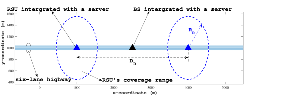
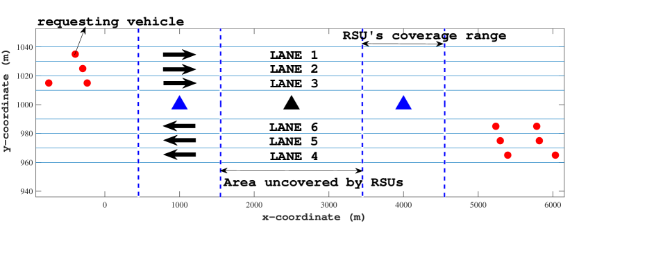
We evaluate the performance of our proposed Algorithm 1 through numerical experiments in MATLAB (ver. 2021b). The experiments are implemented on a PC with an AMD Ryzen 9 5900X@3.7GHz (24 CPUs) core and 32GB of RAM. We consider a six-lane highway with three lanes in each direction, as depicted in Figs. 5 and 5. Similar to [18, 1, 3], we set , , km, m, MB, MB, Gcycles, MHz, s/hop, unit/MB, dBm and GHz. If , then we set MHz, units/MHz, GHz and units/GHz. Otherwise, we set MHz, units/MHz, GHz and units/GHz. We use and . In addition, the time step is set as s. Similar to [7] and [31], the vehicle speeds in lanes , and are set as or , or , and or km/h, respectively.
For a comprehensive comparison, we have to benchmark Algorithm 1 against the most relevant related works in the literature. Different from [17] and [18], those works must design task assignment algorithms for multi-agent environments while allocating autonomous vehicles’ tasks to servers according to their movement in highway scenarios. As a result, we compare Algorithm 1 with the following three algorithms.
-
1.
Exhaustive Search (ES): A centralized algorithm where a central operator collects all network information and finds the globally optimal solution using exhaustive search, similar to [17].
-
2.
Traditional Regret-Matching (TRM) scheme [20]: A distributed algorithm where each player selects an action on the basis of its regret value, and the regret values are not calculated with respect to changes in the vehicular network.
-
3.
Reinforcement Learning with Network-Assisted Feedback (RLNF) scheme [19]: A distributed algorithm where each player selects its action without knowing global network conditions.
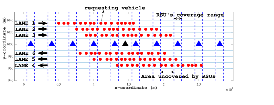
To demonstrate that Algorithm 1 works effectively in not only small-scale but also large-scale environments, we evaluate all the four algorithms in two scenarios. Specifically, in Scenario , there are servers deployed along the highway while vehicles request to complete their tasks. In contrast to Scenario , we increase the number of servers and requesting vehicles to and , respectively, in Scenario . On the other hand, in both scenarios, the requesting vehicles in lanes , and are moving at a speed of , and km/h, respectively. In addition, the inter-RSU distance is set as km.
V-B Simulation Results
Table I compares the performance of Algorithm 1 with the three benchmark schemes. According to the objective function in (13), Algorithm 1 aims to minimize the total delay and cost for task processing; thus, we select the sum of delay and cost as a performance metric. Here, the total delay plus cost and the computation time for task completion are shown for two scenarios, as shown in Figs. 5 and 5. In Scenario , by using servers, Algorithm 1, ES and TRM complete tasks with the lowest total delay plus cost of . Importantly, Algorithm 1 finds the best solution with the smallest computation time of s. This represents a significant reduction of more than % in computation time compared to the next best scheme TRM. Hereby, Algorithm 1 can be applicable to the real deployment scenarios as it satisfies the latency requirement in vehicular applications, i.e. from s to s [32, 33].
In Scenario , the number of servers and tasks is increased up to and , respectively. Given the specifications of a typical PC, it is impossible for ES to iterate through potential solutions. Of the remaining three algorithms, Algorithm 1 converges to the CE solution within the shortest computation time of s, giving the lowest total delay plus cost of . In general, a CE solution might not necessarily be the optimal solution for the BNLP problem (13). Here, we show through experiment results that in most realistic networks, the gap between CE and optimal solution is small (almost negligible) — illustrating that Algorithm 1 provides a good trade off between convergence speed and optimality. It is noted that the TRM and RLNF schemes are not able to perform as well, despite they are also based on RM learning. The reason is that the regret values in the TRM and RLNF schemes are not updated with respect to changes in the operating vehicular environment. Furthermore, since the TRM scheme makes task assignment decisions based on information about global network conditions, its total delay plus cost is lower than that of RLNF.
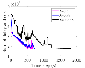
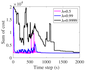
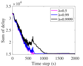
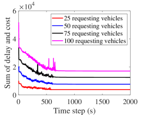
The fast convergence behaviour of the proposed scheme is essential for a dynamic environment in which ITS applications operate. Figs. 6, 8 and 7 illustrate how the convergence of Algorithm 1 depends on the forgetting factor . In addition, Figs. 8 and 7 show the impact of on delay and cost, respectively. As seen, the fastest convergence occurs when decreases from to . At , the cumulative regret of an agent is updated with respect to their instantaneous regret rather than their outdated regret. Furthermore, Fig. 9 shows that such fast convergence is always maintained irrespective of the number of participating agents.
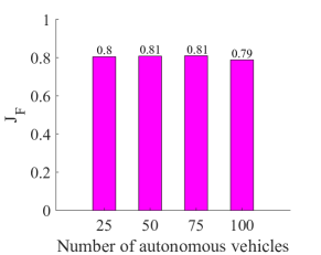
To quantify fairness in terms of utility among agents (autonomous vehicles), we make use of Jain’s fairness index proposed in [34] as follows:
| (19) |
In addition, the utility fairness among the agents would be maintained when the approximate value of is . As shown in Fig. 10, Algorithm 1 achieves the fairness close to , e.g. , even though the autonomous vehicle density is high. Here, to calculate , we employ the value of agents’ utility when Algorithm 1 converges at the correlated equilibrium.
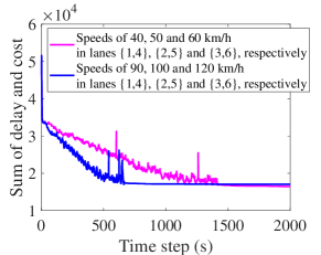
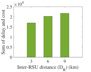
Fig. 11 demonstrates that Algorithm 1 adapts quickly to the environment changes caused by the agents’ mobility. Here, when the agents move at high speeds, it causes a decrease in the duration when they pass through an RSU, or they will enter the next RSUs’ coverage range. Thus, the number of agents’ actions which are able to both minimize the sum of delay and cost, and satisfy constraints in (13) is reduced significantly. Certainly, it would be much less than that of the scenario in which the agents traverse the highway with lower speeds. As a result, the convergence speed of Algorithm 1 in the former is quicker than that in the latter. In particular, Fig. 12 shows the influence of RSU deployment on the performance of our proposed scheme. With the shortest distance between two consecutive RSUs (i.e. km), the RSUs are distributed densely along the six-lane highway. It leads to the lowest total delay and cost achieved by Algorithm 1. Extending the inter-RSU distance will cause an increase in the total delay and cost.
VI Conclusion
To address the issue of limited computation resources in VEC, this paper proposes a task assignment scheme where vehicles’ tasks are migrated across multiple servers according to their mobility pattern. To this end, we have formulated a BNLP problem that minimizes the total delay and cost incurred by the participating vehicles. We then proposed a multi-agent RM learning-based algorithm that is theoretically proved to converge to the CE solution of the formulated problem. The simulation results show the clear advantages of our proposed algorithm over existing solutions.
Proof of Theorem 1
Proof.
For notational convenience, let us drop the subscript and define the following Lyapunov function:333, where is the Euclidean norm.
| (20) |
where represents the negative orthant. Taking the time-derivative of (20) yields
| (21) |
First, we find by rewriting (17) as:
| (22) |
Let be a constant step size. It can be seen that (22) has the form of a constant step size stochastic approximation algorithm and satisfies [35, Th. 17.1.1]. Thus, its dynamics can be characterised by an ordinary differential equation (see [35, Ch. 17] for further details). This means the system can be approximated by replacing with its expected value. By applying [35, Theorem 17.1.1], converges weakly (in distribution) to the averaged system corresponding to (22). As such,
| (23) |
Next, replacing from (23) into (21) gives:
| (24) |
where is an upper bound on , , and is the cardinality of the set (the set of actions of a player ). Note that in the last equality of (24), we have used the following two lemmas:444The proof of Lemma 2 is similar to the proof of Theorem 5.1 in [36], so the proof is omitted here.
Finally, it follows from (24) that by assuming , one can choose a sufficiently small such that
This implies that goes to zero at an exponential rate. Therefore, .
Let be the empirical distribution of the joint action by all players up to the time . It can be defined by a stochastic approximation recursion as:
| (25) |
The elements of the regret matrix in (16) can be rewritten as follows
| (26) |
On the last line of (Proof.), we have substituted from (25). Finally, on any convergent subsequence , we have:
| (27) |
Comparing (27) with the definition of Correlated Equilibrium in Eq. (15) completes the proof. ∎
References
- [1] L. T. Tan and R. Q. Hu, “Mobility-Aware Edge Caching and Computing in Vehicle Networks: A Deep Reinforcement Learning,” IEEE Transactions on Vehicular Technology, vol. 67, no. 11, pp. 10 190–10 203, Nov. 2018.
- [2] L. Silva, N. Magaia, B. Sousa, A. Kobusińska, A. Casimiro, C. X. Mavromoustakis, G. Mastorakis, and V. H. C. de Albuquerque, “Computing Paradigms in Emerging Vehicular Environments: A Review,” IEEE/CAA Journal of Automatica Sinica, vol. 8, no. 3, pp. 491–511, 2021.
- [3] Z. Ning, K. Zhang, X. Wang, M. S. Obaidat, L. Guo, X. Hu, B. Hu, Y. Guo, B. Sadoun, and R. Y. K. Kwok, “Joint Computing and Caching in 5G-Envisioned Internet of Vehicles: A Deep Reinforcement Learning-Based Traffic Control System,” IEEE Transactions on Intelligent Transportation Systems, pp. 1–12, 2020.
- [4] A. Girma, N. Bahadori, M. Sarkar, T. G. Tadewos, M. R. Behnia, M. N. Mahmoud, A. Karimoddini, and A. Homaifar, “IoT-enabled autonomous system collaboration for disaster-area management,” IEEE/CAA Journal of Automatica Sinica, vol. 7, no. 5, pp. 1249–1262, 2020.
- [5] H. Chang, Y. Chen, B. Zhang, and D. Doermann, “Multi-UAV Mobile Edge Computing and Path Planning Platform Based on Reinforcement Learning,” IEEE Transactions on Emerging Topics in Computational Intelligence, vol. 6, no. 3, pp. 489–498, 2022.
- [6] M. Yi, P. Yang, M. Chen, and N. T. Loc, “A DRL-Driven Intelligent Joint Optimization Strategy for Computation Offloading and Resource Allocation in Ubiquitous Edge IoT Systems,” IEEE Transactions on Emerging Topics in Computational Intelligence, pp. 1–16, 2022.
- [7] Transport for NSW, “Traffic Statistics.” [Online]. Available: https://www.rms.nsw.gov.au/about/corporate-publications/statistics/index.html
- [8] J. Bi, H. Yuan, S. Duanmu, M. Zhou, and A. Abusorrah, “Energy-Optimized Partial Computation Offloading in Mobile-Edge Computing With Genetic Simulated-Annealing-Based Particle Swarm Optimization,” IEEE Internet of Things Journal, vol. 8, no. 5, pp. 3774–3785, 2021.
- [9] H. Yuan and M. Zhou, “Profit-Maximized Collaborative Computation Offloading and Resource Allocation in Distributed Cloud and Edge Computing Systems,” IEEE Transactions on Automation Science and Engineering, vol. 18, no. 3, pp. 1277–1287, 2021.
- [10] F. Zeng, Q. Chen, L. Meng, and J. Wu, “Volunteer Assisted Collaborative Offloading and Resource Allocation in Vehicular Edge Computing,” IEEE Transactions on Intelligent Transportation Systems, vol. 22, no. 6, pp. 3247–3257, 2021.
- [11] X. Bai, W. Yan, and S. S. Ge, “Efficient Task Assignment for Multiple Vehicles With Partially Unreachable Target Locations,” IEEE Internet of Things Journal, vol. 8, no. 5, pp. 3730–3742, 2021.
- [12] Z. Zhang, M. Zhou, and J. Wang, “Construction-Based Optimization Approaches to Airline Crew Rostering Problem,” IEEE Transactions on Automation Science and Engineering, vol. 17, no. 3, pp. 1399–1409, 2020.
- [13] Z. Zong, M. Zheng, Y. Li, and D. Jin, “MAPDP: Cooperative Multi-Agent Reinforcement Learning to Solve Pickup and Delivery Problems,” AAAI Conference on Artificial Intelligence, vol. 36, no. 9, pp. 9980–9988, 2022.
- [14] S. Sarkar, V. Gundecha, A. Shmakov, S. Ghorbanpour, A. R. Babu, P. Faraboschi, M. Cocho, A. Pichard, and J. Fievez, “Multi-Agent Reinforcement Learning Controller to Maximize Energy Efficiency for Multi-Generator Industrial Wave Energy Converter,” AAAI Conference on Artificial Intelligence, vol. 36, no. 11, pp. 12 135–12 144, 2022.
- [15] W. Zhan, C. Luo, J. Wang, C. Wang, G. Min, H. Duan, and Q. Zhu, “Deep-Reinforcement-Learning-Based Offloading Scheduling for Vehicular Edge Computing,” IEEE Internet Things J., vol. 7, no. 6, pp. 5449–5465, 2020.
- [16] H. Peng and X. S. Shen, “Deep Reinforcement Learning based Resource Management for Multi-Access Edge Computing in Vehicular Networks,” IEEE Transactions on Network Science and Engineering, pp. 1–1, 2020.
- [17] H. Wang, H. Ke, G. Liu, and W. Sun, “Computation Migration and Resource Allocation in Heterogeneous Vehicular Networks: A Deep Reinforcement Learning Approach,” IEEE Access, vol. 8, pp. 171 140–171 153, 2020.
- [18] Q. Yuan, J. Li, H. Zhou, T. Lin, G. Luo, and X. Shen, “A Joint Service Migration and Mobility Optimization Approach for Vehicular Edge Computing,” IEEE Transactions on Vehicular Technology, vol. 69, no. 8, pp. 9041–9052, 2020.
- [19] D. D. Nguyen, H. X. Nguyen, and L. B. White, “Reinforcement Learning With Network-Assisted Feedback for Heterogeneous RAT Selection,” IEEE Transactions on Wireless Communications, vol. 16, no. 9, pp. 6062–6076, 2017.
- [20] C. Fan, B. Li, C. Zhao, and Y. Liang, “Regret Matching Learning Based Spectrum Reuse in Small Cell Networks,” IEEE Transactions on Vehicular Technology, vol. 69, no. 1, pp. 1060–1064, 2020.
- [21] X. Xu and Q. Zhao, “Distributed No-Regret Learning in Multiagent Systems: Challenges and Recent Developments,” IEEE Signal Processing Magazine, vol. 37, no. 3, pp. 84–91, 2020.
- [22] F. Sentenac, E. Boursier, and V. Perchet, “Decentralized Learning in Online Queuing Systems,” in Advances in Neural Information Processing Systems, vol. 34. Curran Associates, Inc., 2021.
- [23] G. E. Flaspohler, F. Orabona, J. Cohen, S. Mouatadid, M. Oprescu, P. Orenstein, and L. Mackey, “Online Learning with Optimism and Delay,” in 38th International Conference on Machine Learning, ser. Proceedings of Machine Learning Research, vol. 139, 18–24 Jul 2021, pp. 3363–3373.
- [24] I. Bistritz and N. Bambos, “Cooperative Multi-player Bandit Optimization,” in Advances in Neural Information Processing Systems, H. Larochelle, M. Ranzato, R. Hadsell, M. Balcan, and H. Lin, Eds., vol. 33. Curran Associates, Inc., 2020, pp. 2016–2027.
- [25] C. Daskalakis and N. Golowich, “Fast Rates for Nonparametric Online Learning: From Realizability to Learning in Games,” ser. STOC 2022. Association for Computing Machinery, 2022, p. 846–859.
- [26] I. Anagnostides, C. Daskalakis, G. Farina, M. Fishelson, N. Golowich, and T. Sandholm, “Near-Optimal No-Regret Learning for Correlated Equilibria in Multi-Player General-Sum Games,” in 54th Annual ACM SIGACT Symposium on Theory of Computing, 2022, p. 736–749.
- [27] S. Hart and A. Mas-Colell, “A Simple Adaptive Procedure Leading to Correlated Equilibrium,” Econometrica, vol. 68, no. 5, pp. 1127–1150, 2000.
- [28] ——, “A Reinforcement Procedure Leading to Correlated Equilibrium,” in Economics Essays. Berlin: Springer, 2001, pp. 181–200.
- [29] R. J. Aumann, “Correlated Equilibrium as an Expression of Bayesian Rationality,” Econometrica: Journal of the Econometric Society, vol. 55, no. 1, pp. 1–18, Jan 1987.
- [30] S. Hart and D. Schmeidler, “Existence of Correlated Equilibria,” Mathematics of Operations Research, vol. 14, no. 1, pp. 18–25, Feb 1989.
- [31] B. L. Nguyen, D. T. Ngo, M. N. Dao, V. N. Q. Bao, and H. L. Vu, “Scheduling and Power Control for Connectivity Enhancement in Multi-Hop I2V/V2V Networks,” IEEE Transactions on Intelligent Transportation Systems, pp. 1–11, 2021.
- [32] S. Raza, S. Wang, M. Ahmed, and M. R. Anwar, “An Initial Investigation of the Effects of a Fully Automated Vehicle Fleet on Geometric Design,” Wireless Communications and Mobile Computing, vol. 2019, pp. 1–19, 2019.
- [33] S.-C. Lin, Y. Zhang, C.-H. Hsu, M. Skach, M. E. Haque, L. Tang, and J. Mars, “The Architectural Implications of Autonomous Driving: Constraints and Acceleration,” in Twenty-Third International Conference on Architectural Support for Programming Languages and Operating Systems, vol. 53, no. 2, 2018, p. 751–766.
- [34] R. Jain, D. M. Chiu, and W. R. Hawe, “A Quantitative Measure Of Fairness And Discrimination For Resource Allocation In Shared Computer Systems,” ArXiv, vol. cs.NI/9809099, 1998.
- [35] V. Krishnamurthy, Partially Observed Markov Decision Processes From Filtering to Controlled Sensing. Cambridge University Press, 2016.
- [36] D. D. Nguyen, “Adaptive Reinforcement Learning for Heterogeneous Network Selection,” Ph.D. dissertation, The University of Adelaide, 2018.