Stable numerical simulation of Einstein equations
in gravitational collapse space–time

Abstract

We perform simulations in a gravitational collapsing model using the Einstein equations. In this paper, we review the equations for constructing the initial values and the evolution form of the Einstein equations called the BSSN formulation. In addition, since we treat a nonvacuum case, we review the evolution equations of the matter fields of a perfect fluid. To make the simulations stable, we propose a modified system, which decreases numerical errors in analysis, and we actually perform stable simulations with decreased numerical errors.

1 Introduction

Numerical relativity, which solves the Einstein equations numerically, has been widely studied [1, 2, 3, 4]. In particular, for the direct observation of gravitational waves (e.g., [5]), numerical relativity makes important contributions.

Stable numerical simulations are important to clarify the details of phenomena. Since the Einstein equations are the nonlinear partial differential equations, numerical errors tend to accumulate. Although there are some research studies to reduce the numerical errors, they are mainly in the vacuum case. Thus, we suggest a modified system to reduce numerical errors by modifying the evolution equation in a perfect fluid.

The structure of this paper is as follows. We review the space–time decomposition of the Einstein equations in a perfect fluid in Sec. 2. In Sec. 3, we introduce the equations for the numerical simulations of the Einstein equations as the initial value problem in the perfect fluid. We perform some simulations in the dust case and propose a modified system to reduce the numerical errors in Sec. 4. We summarize this paper in Sec. 5. In this paper, indices such as $(\mu,\nu,\lambda,\cdots)$ and $(i,j,k,\cdots)$ run from 0 to 3 and 1 to 3, respectively. We use the Einstein convention of summation of repeated up–down indices.

2 Abstract for numerical simulations of Einstein equations in perfect fluid

The Einstein equations are as follows.

$${}^{(4)}R_{\mu\nu}-\dfrac{1}{2}{}^{(4)}Rg_{\mu\nu}=8\pi T_{\mu\nu},$$ (1)

where $g_{\mu\nu}$ is the four-dimensional metric, ${}^{(4)}R_{\mu\nu}$ is the four-dimensional Ricci tensor, ${}^{(4)}R\equiv g^{\mu\nu}{}^{(4)}R_{\mu\nu}$, $g^{\mu\nu}$ is the inverse of $g_{\mu\nu}$, and $T_{\mu\nu}$ is the stress–energy tensor. Eq. (1) is not a dynamical form because the time and space components are mixed. Generally, we often carry out space–time decomposition of Eq. (1) for performing the simulations.

There are some dynamical forms of Eq. (1), the most basic formulation is the ADM formulation [6, 7]:

$$\partial_{t}\gamma_{ij} =-2\alpha K_{ij}+\gamma_{jm}(D_{i}\beta^{m})+\gamma_{im}(D_{j}\beta^{m}),$$ (2)

$$\partial_{t}K_{ij} =-D_{i}D_{j}\alpha+\alpha R_{ij}+\alpha KK_{ij}-2\alpha\gamma^{mn}K_{mi}K_{nj}$$

$$\quad-8\pi\alpha S_{ij}+4\pi\alpha S\gamma_{ij}-4\pi\alpha\rho_{\text{H}}\gamma_{ij}+\beta^{\ell}(D_{\ell}K_{ij})$$

$$\quad+K_{\ell i}(D_{j}\beta^{\ell})+K_{\ell j}(D_{i}\beta^{\ell}),$$ (3)

$$\mathcal{H} \equiv R+K^{2}-\gamma^{im}\gamma^{nj}K_{ij}K_{mn}-16\pi\rho_{\text{H}}\approx 0,$$ (4)

$$\mathcal{M}_{i} \equiv\gamma^{jm}(D_{j}K_{mi})-D_{i}K-8\pi J_{i}\approx 0,$$ (5)

where $\gamma_{ij}\equiv g_{ij}$ is the induced metric, $\gamma^{ij}$ is the inverse of $\gamma_{ij}$, and $K_{ij}$ is the extrinsic curvature defined as Eq. (2). $\alpha\equiv 1/\sqrt{-g^{00}}$ and $\beta^{i}\equiv\alpha^{2}g^{0i}$ are the lapse function and the shift vector, respectively. $D_{i}$ is the covariant derivative associated with $\gamma_{ij}$, $R_{ij}$ is the Ricci tensor in three dimensions, $K\equiv\gamma^{ij}K_{ij}$, and $R\equiv\gamma^{ij}R_{ij}$. $\rho_{\mathrm{H}}\equiv\alpha^{2}g^{0\mu}g^{0\nu}T_{\mu\nu}$ is the mass density, $J_{i}\equiv\alpha g^{0\mu}T_{\mu i}$ is the momentum density, $S_{ij}\equiv T_{ij}$ is the stress tensor, and $S\equiv\gamma^{ij}S_{ij}$. $\mathcal{H}$ and $\mathcal{M}_{i}$ are the Hamiltonian constraint and the momentum constraint, respectively. The symbol $\approx$ means zero in the mathematical sense but nonzero in the numerical sense.

In the calculation in the nonvacuum case, we also solve the evolution equations of matter fields. These equations are given by the space–time decomposition of $g^{\mu\lambda}(\nabla_{\mu}T_{\lambda\nu})=0$, where $\nabla_{\mu}$ is the covariant derivative associated with $g_{\mu\nu}$. For the perfect fluid case, the stress–energy tensor is given as

$$T_{\mu\nu}=\{\rho(1+\epsilon)+p\}g_{\mu\lambda}g_{\nu\omega}u^{\lambda}u^{\omega}+pg_{\mu\nu},$$ (6)

where $\rho$ is the rest mass, $\epsilon$ is the inner energy, $u^{\mu}$ is the four velocity, and $p$ is the pressure. The evolution equations of $\epsilon$ and $\rho u^{i}$ are given by $g^{\mu\lambda}(\nabla_{\mu}T_{\lambda\nu})=0$. The evolution equation of $\rho$ is given by the continuous equation $\nabla_{\mu}(\rho u^{\mu})=0$. On the other hand, $p$ is usually given by other conditions such as the equation of state.

3 Basic equations

3.1 Equations for initial values

If we set the initial values, they have to satisfy the constraints $\mathcal{H}$ and $\mathcal{M}_{i}$. The dynamical variables $\gamma_{ij}$ and $K_{ij}$ include 12 components because they are symmetric tensors. However, there are only four constraints. Thus, according to [8], we reformulate the constraints such that

$$\hat{\gamma}^{ij}(\hat{D}_{i}\hat{D}_{j}\psi) =\frac{1}{8}\psi\hat{R}+\frac{1}{12}\psi^{5}K^{2}-2\pi\psi^{5}\rho_{\text{H}}$$

$$\quad-\frac{1}{8\psi^{7}}\hat{\gamma}^{im}\hat{\gamma}^{jn}\hat{A}_{ij}\hat{A}_{mn},$$ (7)

$$\hat{\gamma}^{jm}(\hat{D}_{j}\hat{D}_{m}X_{i}) =-\frac{1}{3}\hat{\gamma}^{jm}(\hat{D}_{i}\hat{D}_{j}X_{m})+\frac{2}{3}\psi^{6}(\hat{D}_{i}K)$$

$$\quad-\hat{R}_{ij}\hat{\gamma}^{jm}X_{m}+8\pi\psi^{6}J_{i},$$ (8)

where $\hat{A}_{ij}\equiv\psi^{2}(K_{ij}-(1/3)K\psi^{4}\hat{\gamma}_{ij})$, $\psi$ satisfies relations such as $\gamma_{ij}=\psi^{4}\hat{\gamma}_{ij}$, and $X_{i}$ satisfies the relation $\hat{D}_{i}X_{j}+\hat{D}_{j}X_{i}-(2/3)\hat{\gamma}^{mn}(\hat{D}_{n}X_{m})\hat{\gamma}_{ij}=\hat{A}_{ij}$. $\hat{D}_{i}$ is the covariant derivative associated with $\hat{\gamma}_{ij}$, $\hat{R}_{ij}$ is the Ricci tensor of $\hat{\gamma}^{ij}$, and $\hat{R}\equiv\hat{\gamma}^{ij}\hat{R}_{ij}$. We often assume $\hat{\gamma}_{ij}=\delta_{ij}$ and $K=0$. Then, we set a suitable boundary condition, and we solve Eqs. (7)–(8).

The Einstein equations are not satisfied by simply giving the dynamical variables $(\gamma_{ij},K_{ij})$ at the initial time. We have to give the gauge variables $(\alpha,\beta^{i})$ as appropriate values. For the lapse function $\alpha$, we assume $K=0$ and $\partial_{t}K=0$ in Eqs. (2)–(4), and we obtain

$$\hat{\gamma}^{ij}(\hat{D}_{i}\hat{D}_{j}\alpha) =-2\psi^{-1}\hat{\gamma}^{ij}(\hat{D}_{j}\psi)(\hat{D}_{i}\alpha)+4\pi\alpha\psi^{4}\rho_{\text{H}}$$

$$\quad+\alpha\psi^{-8}\hat{\gamma}^{mi}\hat{\gamma}^{jn}\hat{A}_{ij}\hat{A}_{mn}+4\pi\psi^{4}\alpha S.$$ (9)

This is called the maximal slicing condition [9]. For the shift vector $\beta^{i}$, the minimal distortion gauge condition [7] is often used. We solve the nonlinear elliptic-type Eqs. (7)–(9), obtain $(\psi,\hat{X}_{i},\alpha)$, and then get $(\alpha,\gamma_{ij},K_{ij})$ at the initial time.

3.2 Evolution equations and constraint equations

Since it is well known that the numerical simulations using Eqs. (2)–(3) are unstable, we should reformulate the evolution equations. The BSSN formulation [10, 11] is one of the formulations most commonly used by numerical relativists. The dynamical variables are $(\varphi,K,\tilde{\gamma}_{ij},\tilde{A}_{ij},\tilde{\Gamma}^{i})$ instead of $(\gamma_{ij},K_{ij})$, where $\varphi=(1/12)\log(\text{det}(\gamma_{ij}))$, $\tilde{\gamma}_{ij}=e^{-4\varphi}\gamma_{ij}$, $K=\gamma^{ij}K_{ij}$, $\tilde{A}_{ij}=e^{-4\varphi}(K_{ij}-(1/3)K\gamma_{ij})$, $\tilde{\Gamma}^{\ell}=\tilde{\Gamma}^{\ell}{}_{ij}\tilde{\gamma}^{ij}$, $\tilde{\gamma}^{ij}$ is the inverse of $\tilde{\gamma}_{ij}$, and $\tilde{\Gamma}^{\ell}{}_{ij}$ is the connection coefficient of $\tilde{\gamma}_{ij}$. The evolution equations are

$$\partial_{t}\varphi =-\frac{1}{6}\alpha K+\frac{1}{6}(\partial_{i}\beta^{i})+\beta^{i}(\partial_{i}\varphi),$$ (10)

$$\partial_{t}K =-(D_{i}D_{j}\alpha)e^{-4\varphi}\tilde{\gamma}^{ij}+\frac{1}{3}\alpha K^{2}+4\pi\alpha S$$

$$\quad+\alpha\tilde{A}_{ij}\tilde{A}_{mn}\tilde{\gamma}^{im}\tilde{\gamma}^{jn}+4\pi\alpha\rho_{\text{H}}+\beta^{i}(\partial_{i}K),$$ (11)

$$\partial_{t}\tilde{\gamma}_{ij} =-2\alpha\tilde{A}_{ij}-\frac{2}{3}(\partial_{\ell}\beta^{\ell})\tilde{\gamma}_{ij}+(\partial_{i}\beta^{\ell})\tilde{\gamma}_{\ell j}+(\partial_{j}\beta^{\ell})\tilde{\gamma}_{\ell i}$$

$$\quad+\beta^{\ell}(\partial_{\ell}\gamma_{ij}),$$ (12)

$$\partial_{t}\tilde{A}_{ij} =-(D_{i}D_{j}\alpha)^{\rm TF}e^{-4\varphi}-2\alpha\tilde{A}_{im}\tilde{A}_{jn}\tilde{\gamma}^{mn}+\alpha K\tilde{A}_{ij}$$

$$\quad+\alpha e^{-4\varphi}R^{\rm TF}_{ij}-8\pi\alpha e^{-4\varphi}S_{ij}^{\rm TF}-\dfrac{2}{3}(\partial_{\ell}\beta^{\ell})\tilde{A}_{ij}$$

$$\quad+(\partial_{i}\beta^{\ell})\tilde{A}_{\ell j}+(\partial_{j}\beta^{\ell})\tilde{A}_{\ell i}+\beta^{\ell}(\partial_{\ell}\tilde{A}_{ij}),$$ (13)

$$\partial_{t}\tilde{\Gamma}^{\ell} =-2(\partial_{i}\alpha)\tilde{A}_{mj}\tilde{\gamma}^{ij}\tilde{\gamma}^{m\ell}+2\alpha\tilde{\Gamma}^{\ell}{}_{mn}\tilde{A}_{ij}\tilde{\gamma}^{mi}\tilde{\gamma}^{nj}$$

$$\quad+12\alpha(\partial_{i}\varphi)\tilde{A}^{i\ell}-\dfrac{4}{3}\alpha\tilde{\gamma}^{\ell i}(\partial_{i}K)-16\pi\alpha\tilde{\gamma}^{i\ell}J_{i}$$

$$\quad+\dfrac{1}{3}(\partial_{i}\partial_{j}\beta^{j})\tilde{\gamma}^{\ell i}+(\partial_{i}\partial_{j}\beta^{\ell})\tilde{\gamma}^{ij}+\dfrac{2}{3}(\partial_{i}\beta^{i})\tilde{\Gamma}^{\ell}$$

$$\quad-(\partial_{i}\beta^{\ell})\tilde{\Gamma}^{i}+\beta^{i}(\partial_{i}\tilde{\Gamma}^{\ell}),$$ (14)

where $R_{ij}$ in the above is defined as

$$R_{ij} \equiv-\frac{1}{2}\tilde{\gamma}^{\ell m}(\partial_{\ell}\partial_{m}\tilde{\gamma}_{ij})+\dfrac{1}{2}\tilde{\gamma}_{mi}(\partial_{j}\tilde{\Gamma}^{m})+\dfrac{1}{2}\tilde{\gamma}_{mj}(\partial_{i}\tilde{\Gamma}^{m})$$

$$\quad+\dfrac{1}{2}\tilde{\gamma}_{i\ell}\tilde{\Gamma}^{\ell}{}_{jm}\tilde{\Gamma}^{m}+\dfrac{1}{2}\tilde{\gamma}_{j\ell}\tilde{\Gamma}^{\ell}{}_{im}\tilde{\Gamma}^{m}+\tilde{\gamma}^{mn}\tilde{\gamma}_{\ell k}\tilde{\Gamma}^{\ell}{}_{nj}\tilde{\Gamma}^{k}{}_{mi}$$

$$\quad+\tilde{\gamma}^{mn}\tilde{\gamma}_{kj}\tilde{\Gamma}^{\ell}{}_{ni}\tilde{\Gamma}^{k}{}_{\ell m}+\tilde{\gamma}^{mn}\tilde{\gamma}_{ki}\tilde{\Gamma}^{\ell}{}_{nj}\tilde{\Gamma}^{k}{}_{\ell m}$$

$$\quad-2(\tilde{D}_{j}\tilde{D}_{i}\varphi)-2\tilde{\gamma}^{mn}(\tilde{D}_{m}\tilde{D}_{n}\varphi)\tilde{\gamma}_{ij}+4(\tilde{D}_{i}\varphi)(\tilde{D}_{j}\varphi)$$

$$\quad-4\tilde{\gamma}^{mn}(\tilde{D}_{m}\varphi)(\tilde{D}_{n}\varphi)\tilde{\gamma}_{ij}.$$ (15)

The symbol ^TF means the trace-free part of the value, and $\tilde{D}_{i}$ is the covariant derivative associated with $\tilde{\gamma}_{ij}$. The constraint equations are

$$\tilde{\mathcal{H}} \equiv R+\frac{2}{3}K^{2}-\tilde{A}_{ij}\tilde{A}_{mn}\tilde{\gamma}^{im}\tilde{\gamma}^{jn}-16\pi\rho_{\text{H}}\approx 0,$$ (16)

$$\tilde{\mathcal{M}}_{i} \equiv\tilde{\gamma}^{jn}(\tilde{D}_{j}\tilde{A}_{ni})+6(\tilde{D}_{j}\varphi)\tilde{\gamma}^{jn}\tilde{A}_{ni}-\frac{2}{3}\tilde{D}_{i}K$$

$$\quad-8\pi J_{i}\approx 0,$$ (17)

$$\tilde{\mathcal{S}} \equiv\text{det}(\tilde{\gamma}_{ij})-1\approx 0,$$ (18)

$$\tilde{\mathcal{A}} \equiv\tilde{\gamma}^{ij}\tilde{A}_{ij}\approx 0,$$ (19)

$$\tilde{\mathcal{G}}^{\ell} \equiv\tilde{\Gamma}^{\ell}-\tilde{\Gamma}^{\ell}{}_{ij}\tilde{\gamma}^{ij}\approx 0.$$ (20)

Recently, other formulations have also been used [12, 13] by numerical relativists.

3.3 Evolution equations of matter fields

For the perfect fluid, the evolution equations of matter fields [14] are given by the space–time decomposition of $\nabla_{\mu}(\rho u^{\mu})=0$ and $g^{\mu\lambda}(\nabla_{\mu}T_{\lambda\nu})=0$ as

$$\partial_{t}\rho_{*} =-\partial_{i}(\rho_{*}v^{i}),$$ (21)

$$\partial_{t}e_{*} =-\partial_{i}(e_{*}v^{i}),$$ (22)

$$\partial_{t}(\rho_{*}\hat{u}_{i}) =-\partial_{j}\left(\rho_{*}\hat{u}_{i}v^{j}\right)-\alpha e^{6\varphi}(\partial_{i}p)-\rho_{*}(\partial_{i}\alpha)hw$$

$$\quad+\rho_{*}(\partial_{i}\beta^{n})\hat{u}_{n}-\frac{1}{2hw}\rho_{*}\alpha e^{-4\varphi}(\partial_{i}\tilde{\gamma}^{mn})\hat{u}_{m}\hat{u}_{n}$$

$$\quad+2h(w^{2}-1)w^{-1}\rho_{*}\alpha(\partial_{i}\varphi),$$ (23)

where $\rho_{*}\equiv\rho we^{6\varphi}$, $w\equiv\alpha u^{0}$, $e_{*}\equiv(\rho\epsilon)^{1/\Gamma}e^{6\varphi}w$, $v^{i}\equiv u^{i}/u^{0}$, $h\equiv 1+\epsilon+p/\rho$, $\hat{u}_{i}\equiv he^{-4\varphi}\tilde{\gamma}_{ij}(u^{0}\beta^{j}+u^{j})$, and $\Gamma$ is a constant. In addition, we assume $p=(\Gamma-1)\rho\epsilon$. The relations between $(\rho_{\text{H}},J_{i},S_{ij})$ and $(\rho_{*},e_{*},\hat{u}_{i})$ are

$$\rho_{\text{H}} =e^{-6\varphi}h\rho_{*}w-p,$$ (24)

$$J_{i} =\rho_{*}\hat{u}_{i}e^{-6\varphi},$$ (25)

$$S_{ij} =e^{-6\varphi}w^{-1}h^{-1}\rho_{*}\hat{u}_{i}\hat{u}_{j}+pe^{4\varphi}\tilde{\gamma}_{ij}.$$ (26)

Since the four velocity $u^{\mu}$ is satisfied in the relation $u^{\mu}u_{\mu}=-1$, $w$ is given as $w=\sqrt{1+h^{-2}e^{-4\varphi}\tilde{\gamma}^{ij}\hat{u}_{i}\hat{u}_{j}}$. In addition, for $p=(\Gamma-1)\rho\epsilon$, $h$ is given as $h=1+\Gamma e_{*}\rho_{*}^{-1}(e_{*}w^{-1}e^{-6\varphi})^{\Gamma-1}$.

4 Numerical simulations

In the dust case, we solve the Einstein equations and the matter evolution equations. With reference to [14], we set the initial data as follows.

$$\rho_{*}=a\left(1+\exp\left(\dfrac{r^{2}-r_{0}^{2}}{\delta r^{2}}\right)\right)^{-1},$$ (27)

where $a$ is the gravitational mass $M_{g}=\int d^{3}x(\rho_{\text{H}}\psi^{5}+(1/16\pi)\psi^{-7}\hat{A}_{ij}\hat{A}_{mn}\hat{\gamma}^{im}\hat{\gamma}^{jn})$ as the unit at the initial time and $r=\sqrt{x^{2}+y^{2}+z^{2}}$. This time, we set $a=4.129\times 10^{-3}$, $\delta r^{2}=0.18M_{g}^{2}$, and $r_{0}=4.0M_{g}$. The numerical ranges are $-9\leq x,y,z\leq 9$. This case is static at the initial time, so we set $X_{i}=\hat{A}_{ij}=J_{i}=\beta^{i}=u^{i}=0$. In the dust case, we set the inner energy as $\epsilon=0$ and the pressure $p=0$. We assume $\hat{\gamma}_{ij}=\delta_{ij}$ and $K=0$. Then, the extrinsic curvature $K_{ij}=0$ and $\hat{R}=0$. We obtain the initial data $(\alpha,\gamma_{ij})$ with the above conditions by solving Eqs. (7) and (9). With reference to the Schwarzschild metric, the initial step values of $\psi$ and $\alpha$ are set as $1+1/(1+6r)$ and $1-1/(3/2+r)$, respectively.

Recently, the maximal slicing condition, Eq. (9), and the minimal distortion gauge condition are almost never used in the evolution because the numerical costs are high. The evolution equation of $\alpha$ often uses the $1+\log$ slicing condition [15],

$$\partial_{t}\alpha=-2\alpha K.$$ (28)

Since this condition has the characteristic of singularity avoidance, it is widely used in the simulations for the gravitational collapse models. We choose $\beta^{i}=0$. For the rotating models of neutron stars and/or black holes, the Gamma-driver condition [16] is often used in the evolution equations of $\beta^{i}$.

This time, we select the grid as $\Delta x=\Delta y=\Delta z=1/60$, $\Delta t=1/240$, and the boundary condition as the approximate asymptotic flat boundary. We use the fourth-order Runge–Kutta scheme with mainly the second-order centered space difference. However, for only the advection term, which is the first term on the right-hand side in each of Eqs. (21)–(23), we use the second-order upwind scheme. The direction is defined by the signature of the velocity $v^{i}$.

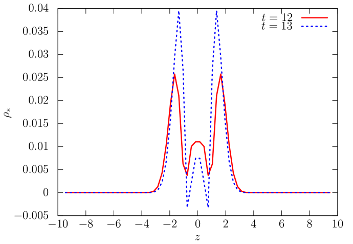
Figure 1: $\rho_{*}$ of $x=y=-0.45$ obtained by solving Eqs. (10)–(14), Eqs. (21)–(23), and Eq. (28). The horizontal line is $z$, the vertical line is $\rho_{*}$. The line of $t=12$ satisfies $\rho_{*}\geq 0$. On the other hand, we see that $\rho_{*}<0$ in $-2<z<2$ at $t=13$.

Fig. 1 shows the weighted rest mass $\rho_{*}$ at $t=12$ and $t=13$ obtained by solving Eqs. (10)–(14), Eqs. (21)–(23), and Eq. (28). We see that $\rho_{*}<0$ at $t=13$ in the $-2<z<2$ range. We check $\rho_{*}\geq 0$ during $0\leq t\leq 12$ in all the simulation ranges. Since $\rho_{*}\geq 0$ is a necessary condition for successful simulations, this simulation fails after $t=13$.

For more stable simulations, we modify Eq. (23) as

$$\partial_{t}(\rho_{*}\hat{u}_{i}) =[\text{Original terms}]+\kappa\rho_{*}\tilde{\gamma}^{mn}(\partial_{m}\partial_{n}\tilde{\mathcal{M}}_{i}),$$ (29)

where $\kappa$ is a damping parameter. This modification is based on the following ideas. By using this modification, we obtain the following: (i) the positive rest mass condition $\rho_{*}\geq 0$ is satisfied, (ii) the constraints, Eqs. (16)–(20), are conserved, and (iii) the total weighted rest mass

$$I=\int\rho_{*}d^{3}x$$ (30)

is conserved. The negative sign of $\kappa$ makes the simulations stable because the dynamical equations of $\tilde{\mathcal{M}}_{i}$ become

$$\partial_{t}\tilde{\mathcal{M}}_{i} =[\text{Original terms}]-\dfrac{8\pi\kappa\rho_{*}}{e^{6\varphi}w}\tilde{\gamma}^{mn}(\partial_{m}\partial_{n}\tilde{\mathcal{M}}_{i})$$ (31)

because of the adjusted terms of Eq. (29). The adjusted term of Eq. (31) has the dissipation effect if $\kappa<0$ because $\rho_{*}/(e^{6\varphi}w)\geq 0$. The set of Eqs. (10)–(14), Eqs. (21)–(22), Eq. (28), and Eq. (29) is called as the modified system hereafter.

Figure 2: $\rho_{*}$ of $x=y=-0.45$ with Eq. (29) and the other conditions are the same as those in Fig. 1. We set the damping parameter of Eq. (29) as $\kappa=-0.1$. The solid line for $t=17$ satisfies $\rho_{*}\geq 0$. On the other hand, we see $\rho_{*}<0$ in $-2<z<2$ at $t=18$.

We show the numerical results of $\rho_{*}$ obtained using the modified system in Fig. 2. The numerical settings are consistent with those in Fig. 1 without the evolution equation of $\rho_{*}\hat{u}_{i}$ and we set $\kappa=-0.1$. For this simulation, we check $\rho_{*}\geq 0$ during $0\leq t\leq 17$ in all simulation ranges. In Fig. 3, we show the L2 norm of the following values:

$$\mathcal{C}^{2}=\tilde{\mathcal{H}}^{2}+\tilde{\gamma}^{ij}\tilde{\mathcal{M}}_{i}\tilde{\mathcal{M}}_{j}+\tilde{\gamma}_{ij}\tilde{\mathcal{G}}^{i}\tilde{\mathcal{G}}^{j}+\tilde{\mathcal{S}}^{2}+\tilde{\mathcal{A}}^{2}.$$ (32)

We see that the norm of the constraints $\mathcal{C}^{2}$ with $\kappa=-0.1$ is less than those in other cases until $0\leq t\leq 17$. On the other hand, the norm with $\kappa=0.1$ is larger than those in other cases. Thus, these results are consistent with the analytical results using Eq. (31). Fig. 4 shows the relative errors against the initial values of the total weighted mass $I$ in Eq. (30). They are not markedly different between the cases of $\kappa=0.0$ and $\kappa=-0.1$.

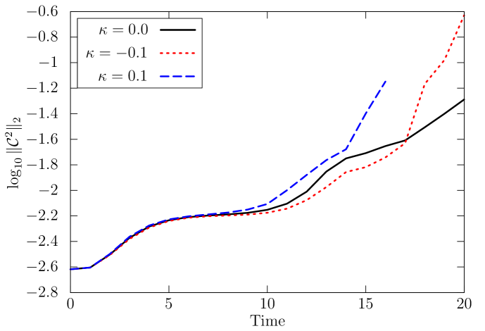
Figure 3: The lines show the constraint errors in the cases of $\kappa=0.0$, $-0.1$, and $0.1$. The horizontal axis is time, and the vertical axis is the logarithm of the L2 norm of $\mathcal{C}^{2}$, Eq. (32).

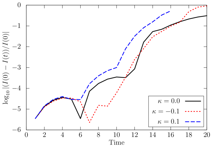
Figure 4: The lines show the relative errors of the total weighted rest mass $I$ in Eq. (30) against the initial values $I(0)$ for the cases of $\kappa=0.0$, $-0.1$, and $0.1$. The horizontal axis is time, and the vertical axis is the logarithm of $|(I(0)-I(t))/I(0)|$.

5 Summary

We reviewed the equations for construction of the initial values, the dynamical equations of the Einstein equations called the BSSN formulation, and the dynamical equations of the matter fields in the perfect fluid. With these equations, we performed the simulations in the dust case. We modified the system by modifying the evolution equations of the matter field, investigated the stability analytically, and performed the simulations with the modified system to confirm the consistency of the analytical results. In addition, the lifetime of the simulations was extended from $t=12$ to $t=17$ with the modification.

References

- [1] M. Alcubierre, Introduction to Numerical Relativity, Oxford Science Publications, Oxford, 2008.
- [2] T. W. Baumgarte and S. L. Shapiro, Numerical Relativity, Cambridge University Press, England, 2010.
- [3] É. Gourgoulhon, Formalism in General Relativity, Springer, Berlin, 2012.
- [4] M. Shibata, Numerical Relativity, World Scientific, Singapore, 2015.
- [5] B. P. Abbott et al., Observation of gravitational waves from a binary black hole merger, Phys. Rev. Lett., 116 (2016), 061102.
- [6] R. Arnowitt et al., Republication of: The dynamics of general relativity, Gen. Relativ. Gravit., 40 (2008), 1997?2027.
- [7] L. Smarr and J. W. York, Jr., Kinematical conditions in the construction of spacetime, Phys. Rev. D, 17 (1978), 2529?2551.
- [8] N. Ó Murchadha and J. W. York, Jr., Initial-value problem of general relativity. I, Phys. Rev. D, 10 (1974), 428–436.
- [9] F. Estabrook et al., Maximally slicing a black hole, Phys. Rev. D, 7 (1973), 2814–2817.
- [10] M. Shibata and T. Nakamura, Evolution of three-dimensional gravitational waves: Harmonic slicing case, Phys. Rev. D, 52 (1995), 5428–5444.
- [11] T. W. Baumgarte and S. L. Shapiro, Numerical integration of Einstein’s field equations, Phys. Rev. D, 59 (1997), 024007.
- [12] J. D. Brown, Covariant formulations of Baumgarte, Shapiro, Shibata, and Nakamura and the standard gauge, Phys. Rev. D, 79 (2009), 104029.
- [13] D. Alic et al., Conformal and covariant formulation of the Z4 system with constraint-violation damping, Phys. Rev. D, 85 (2012), 064040.
- [14] M. Shibata, Fully general relativistic simulation of coalescing binary neutron stars: Preparatory tests, Phys. Rev. D, 60 (1999), 104052.
- [15] C. Bona et al., New formalism for numerical relativity, Phys. Rev. Lett., 75 (1995), 600–603.
- [16] M. Alcubierre et al., Gauge conditions for long-term numerical black hole evolutions without excision, Phys. Rev. D, 67 (2003), 084023.