IAE-Net: Integral Autoencoders for Discretization-Invariant Learning

Abstract

Discretization invariant learning aims at learning in the infinite-dimensional function spaces with the capacity to process heterogeneous discrete representations of functions as inputs and/or outputs of a learning model. This paper proposes a novel deep learning framework based on integral autoencoders (IAE-Net) for discretization invariant learning. The basic building block of IAE-Net consists of an encoder and a decoder as integral transforms with data-driven kernels, and a fully connected neural network between the encoder and decoder. This basic building block is applied in parallel in a wide multi-channel structure, which is repeatedly composed to form a deep and densely connected neural network with skip connections as IAE-Net. IAE-Net is trained with randomized data augmentation that generates training data with heterogeneous structures to facilitate the performance of discretization invariant learning. The proposed IAE-Net is tested with various applications in predictive data science, solving forward and inverse problems in scientific computing, and signal/image processing. Compared with alternatives in the literature, IAE-Net achieves state-of-the-art performance in existing applications and creates a wide range of new applications where existing methods fail.

Keywords Discretization Invariant $\cdot$ Integral Autoencoder $\cdot$ Randomized Data Augmentation $\cdot$ Predictive Data Science $\cdot$ Forward and Inverse Problems, Signal/Image Processing.

1 Introduction

Deep learning was originally proposed with neural networks (NN) parametrizing mappings from a vector space $X\subset\mathbb{R}^{d_{X}}$ to another vector space $Y\subset\mathbb{R}^{d_{Y}}$. In this learning setting, deep learning has become very successful in various applications not just limited to computer science. In many applications, the input space $X\subset\mathbb{R}^{d_{X}}$ and/or the output space $Y\subset\mathbb{R}^{d_{Y}}$ come from the discretization of infinite-dimensional function spaces. Therefore, NNs trained with fixed discrete spaces $X\subset\mathbb{R}^{d_{X}}$ and $Y\subset\mathbb{R}^{d_{Y}}$ cannot be applied to other discrete spaces associated with other discretization formats. For example, let $\mathcal{X}$ denote a Hilbert space of functions defined on $\Omega_{x}=[0,1]^{d_{x}}$ and let $\mathcal{Y}$ denote a Hilbert space of functions defined on $\Omega_{y}=[0,1]^{d_{y}}$. The goal is to learn a mapping $\Psi:\mathcal{X}\rightarrow\mathcal{Y}$. In the numerical implementation, for a fixed set of samples $\{x_{1},\dots,x_{d_{X}}\}\subset[0,1]^{d_{x}}$, let $X=\{\bar{u}\in\mathbb{R}^{d_{X}}:\bar{u}_{i}=u(x_{i}),u\in\mathcal{X}\}$; for a fixed set of samples $\{y_{1},\dots,y_{d_{Y}}\}\subset[0,1]^{d_{y}}$, let $Y=\{\bar{v}\in\mathbb{R}^{d_{Y}}:\bar{v}_{i}=v(y_{i}),v\in\mathcal{Y}\}$. Then learning $\Psi:\mathcal{X}\rightarrow\mathcal{Y}$ is reduced to learning $\bar{\Psi}:X\rightarrow Y$, where an NN $\Psi^{n}(\bar{u};\theta)$ with parameters $\theta$ is trained to approximate $\bar{\Psi}(\bar{u})$ for all $\bar{u}\in X$ in existing deep learning methods. In this sense, $\Psi^{n}(\bar{u};\theta)$ infers a good discrete representation of $\Psi(u)$. However, $\Psi^{n}$ cannot be applied to an arbitrary discrete representation of $u\in\mathcal{X}$, especially when $u$ has a discrete representation of dimension different to $d_{X}$. Similarly, the NN $\Psi^{n}$ cannot infer $v=\Psi(u)$ in an arbitrary discretization format. However, heterogeneous data structures are ubiquitous due to data sensing and collection constraints and, therefore, it is crucially important to design discretization-invariant learning. The goal of this paper is to show that:

• Discretization invariance is achievable for mathematically well-posed problems even with simple interpolation techniques, but IAE-Net achieves the state-of-the-art accuracy.

• Existing methods fail to achieve discretization invariance for ill-posed and highly oscillatory problems, while IAE-Net succeed with reasonablly good accuracy.

There are several immediate solutions to deal with heterogeneous data structures. Typically, expensive re-training is conducted to train a new NN for different discretization formats. However, re-training sometimes would be too expensive for large-scale NNs, or training samples from a certain discrete format might be too limited to obtain good accuracy. Another simple idea is to pre-process the input data and post-process the output data, e.g., using resizing, padding, interpolation [1], or cropping [2] to make data fit the specific requirement of an NN model. However, the numerical accuracy of these simple methods is not satisfactory in challenging applications as we shall see in the numerical experiments. Resizing signals/images to a specific size without deforming patterns contained therein is a major challenge. There are two cases in resizing: downsampling and upscaling. Downsampling may significantly reduce the vital features of data and make it more challenging to learn. Upscaling may generate side effects that mislead NNs.

The above drawbacks have motivated the development of advanced frameworks for discretization-invariant learning recently. There are two main advanced ideas to achieve discretization-invariant transforms in deep learning. The first one is to apply “pointwise" linear transforms in deep neural networks. Traditionally, a linear transform in NNs is a matrix-vector multiplication with a fixed matrix size, and, hence, the linear transform cannot be applied to input vectors with different dimensions, resulting in discretization dependence. The pointwise linear transform to a vector $\bar{u}\in\mathbb{R}^{d_{X}}$ is to apply the same linear transform to each entry of $\bar{u}$ so that the numerical computation can still be implemented for different dimension $d_{X}$’s. This technique is widely used in natural language processing, e.g., the transformer [3] and its variants [4, 5, 6, 7, 8], recurrent architectures [9, 10, 11, 12, 13], and is recently applied to scientific computing for solving parametric partial differential equations (PDEs) and initial value problems [14, 15, 16].

Another approach is to apply a parametrized linear integral transformation in NNs, e.g., $v(y)=\int_{\Omega_{x}}K(x,y;\theta)u(x)dx$ as a linear transformation from $u$ to $v$ in each layer of a deep NN, where $K(x,y;\theta)$ is an integral kernel parametrized with $\theta$. The integral can be implemented independent of the discretization of $u(x)$ so that the integral transform can be applied to arbitrary discrete representation $\bar{u}\in\mathbb{R}^{d_{X}}$ of $u(x)\in\mathcal{X}$, i.e., $d_{X}$ is allowed to be different. Purely convolutional NNs [17, 18, 19, 20, 21, 22] without any fully connected layers fall into this approach, where the integral kernel is a convolutional kernel parametrized by a few parameters. NNs have also been applied to parametrize $K(x,y;\theta)$ for image classification and learning the mathematical operators to solve parametric PDEs and initial value problems [23, 24, 25, 26, 14, 27, 28, 29, 30].

There have been mainly two research directions to theoretically investigate discretization invariant learning, especially for learning an operator from an infinite-dimensional space to another. In terms of approximation theory for operators, based on the universal approximation theory of operators [23] and the quantitative deep network approximation theory [31, 32, 33, 34, 35], there have been several works explaining the power of deep neural networks for approximating operators quantitatively [36, 37, 38, 39, 40]. Especially in certain scientific computing problems, it was shown by [41] that deep network approximation for solution operators mapping low-dimensional functions to another has no curse of dimensionality, even if the function spaces are infinite-dimensional. Going one step further to the generalization error analysis of neural network based operator learning, leveraging recent theories [42, 43, 44, 45, 46, 47, 48, 49, 50], there has been a posteriori and a priori generalization error analysis for learning nonlinear operators with discretization invariance by [38] and [40], respectively.

Although discretization-invariant learning has been explored in the seminal works summarized above, these methods seem to focus on mathematically well-posed problems with non-oscillatory data, and cannot be applied to either ill-posed learning problems or problems with highly oscillatory data. This motivates the design of IAE-Net as a universal discretization-invariant learning framework for both well-posed and ill-posed problems with various data patterns. Besides the state-of-the-art accuracy in existing applications, IAE-Net has broad applications in science and engineering that existing methods are not capable of. For example, other than solving parametric PDEs [24, 14, 51, 22], in inverse scattering problems [52, 53], it is interesting to learn an operator mapping the observed data function space to the parametric function space that models the underlying PDE for high-frequency phenomena. In imaging science [54], an imaging process is to construct a nonlinear operator from the observed data function space to the reconstructed image function space. In image processing problems, e.g., image super-resolution [55], image denoising [19, 56], image inpainting [57], the interest is to learn operators from an image discretized from one function to another. In signal processing, it is a fundamental problem to learn a nonlinear operator mapping a signal function to another or several signal functions [58, 59, 60, 61, 62, 63, 64].

In terms of technical innovation, there are four novel ideas in the design and training of IAE-Net to achieve state-of-the-art accuracy and broaden the application of discretization invariant learning to challenging problems. The main innovation can be summarized below.

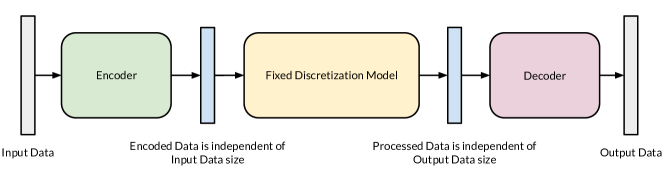
Figure 1: The visualization of a discretization invariant integral autoencoder structure. The design will be described in Section 2.3.1.

1. For the first time, we introduce a data-driven integral autoencoder (IAE), as visualized in Figure 1, to achieve two important goals simultaneously: 1) IAE is discretization invariant via novel nonlinear integral transforms as the encoder and decoder; 2) IAE can capture the low-dimensional or low-complexity structure of a learning task for dimension reduction in the same spirit of data-driven principle component analysis (PCA). The integral kernels in these integral transforms are parametrized by NNs and trained to map functions in an infinite-dimensional space to a low and finite dimensional vector space (or vice versa). The nonlinearity, as oppose to linear integral transforms in existing works, is a key to improve performance. Due to the powerful expressiveness of NNs, these integral transforms could be trained to mimic useful transforms in mathematical analysis, e.g., the Fourier transform [65], wavelet transforms [66, 67, 68, 69], nonlinear PCA [70, 71], etc.

2. To make IAE-Net capable of solving problems with oscillatory phenomena, IAEs are applied in parallel, forming a multi-channel IAE block as shown in Figure 2. Each channel has an IAE applied to data in a certain transformed domain. For example, Figure 2 shows an example of two IAEs, one of which is applied to map functions in their original domain, and the other one of which is applied to map functions in the frequency domain after Fourier transform. This multi-channel IAE structure can be extended to have AEs in different domains inspired by problem-dependent physical models.

3. Inspired by DenseNet [72], by composing multi-channel IAE blocks with pointwise linear transforms as skip connections, a discretization-invariant densely connected structure is proposed as our final IAE-Net visualized in Figure 4. IAE-Net enjoys similar properties of the original DenseNet [72] to boost the learning performance: lessening the gradient vanishing issue, diversifying the features of the inputs of each IAE block, and maximizing the gradient flow information of each IAE block directly to the final loss function.

4. IAE-Net is trained with randomized data augmentation that generates training data with heterogeneous structures to facilitate the performance of discretization invariant learning. In each iteration of the stochastic gradient descent (SGD) for training IAE-Net, the selected training samples are augmented with a set of samples randomly extrapolated/interpolated from the selected samples. This new data augmentation can be understood as a randomized loss function with a random extrapolation/interpolation operator with an image consisting of all possible discrete representations of the training data.

In terms of scientific applications, IAE-Net can be applied not only to traditional machine learning problems, e.g., signal and image processing, classification, prediction, etc, but also to newly emerged scientific machine learning problems, e.g., solving PDEs, solving inverse problems, etc. In the literature of discretization invariant learning, existing algorithms [14, 15] can only be applied to solve well-posed problems, e.g., initial value problems and parametric PDEs, aiming at a small zero-shot generalization error, i.e., NNs trained with data discretized from a fixed format can also be applied to other data with different discretization formats. Table 1 compares the properties and performance of IAE-Net against the baseline models used in this paper. In this paper, we explore the application of IAE-Net to one more situation: the training data are generated with different discretization formats and each format is only applied to generate a small set of training data. This new setting is to simulate the computational environment of many data science problems with heterogeneous training data due to data sensing and collection constraints. Learning in this new setting can also alleviate data cleaning difficulty and cost in data science.

Table 1: Comparison of different DNNs. ResNet: [73]. DeepOnet: [23, 24]. Fourier Neural Operator (FNO): [14]. Fourier Transformer (FT), Galerkin Transformer (GT): [15]. IAE-Net: designed in this proposal. "Yes" means $L2$ relative error (Equation 15) is lower than $10\%$ for the trained resolution; otherwise, we mark "No". DeepONet is labelled ^† as it is discretization invariant and can handle irregular grids only for the output, but not the input.

Model	Discretization	Irregular	Predic-	Solve	Inverse	Image	Signal
	Invariance	Grids	tion	PDE	Problem	Process	Process
ResNet	No	No	Yes	Yes	Yes	Yes	No
DeepONet†	No	No	Yes	Yes	No	No	No
FNO	Yes	No	Yes	Yes	No	No	No
FT	Yes	No	Yes	Yes	No	No	No
GT	Yes	No	Yes	Yes	No	No	No
IAE-Net	Yes	Yes	Yes	Yes	Yes	Yes	Yes

In terms of computational methodologies, IAE-Net can be considered as an algorithm compression technique that can transform the research goal of computational science in many applications. For example, in scientific computing, solving inverse problems accurately and efficiently is still an active research field. Once trained, IAE-Net can solve inverse problems rapidly with a few matrix-vector multiplications. Therefore, it may be sufficient to focus on designing accurate algorithms for inverse problems without much attention to the computational efficiency. These accurate algorithms can generate training data for IAE-Net, and the trained IAE-Net can predict output solutions of these algorithms efficiently, in which sense IAE-Net is a compressed and accelerated version of a slow but accurate algorithm.

We have focused on discretization invariant learning from one function space to another. It is easy to generalize IAE-Net to learn a mapping from a function space to a finite dimensional vector space, or a mapping from a finite dimensional vector space to a function space, by composing IAE-NET with a fixed-size NN. The rest of this paper is organized as follows. IAE-Net and its training algorithm will be introduced in detail in Section 2. Section 3 presents the experimental design and results for the applications covered in this paper. We conclude this paper with a short discussion in Section 4.

Figure 2: A $2$-channel IAE block with a pointwise MLP for merging parallel channels to implement Equation (12). The design will be described in Section 2.3.2.

2 Algorithm Description

This section presents the detailed description of the design of IAE-Net.

2.1 Problem Statement

IAE-Net targets general applications involving the task of learning an objective mapping $\Psi:\mathcal{X}\rightarrow\mathcal{Y}$, where $\mathcal{X}$ and $\mathcal{Y}$ are appropriate function spaces defined on $\Omega_{x}=[0,1]^{d_{x}}$ and $\Omega_{y}=[0,1]^{d_{y}}$ respectively. Here, $d_{x}$ and $d_{y}$ represent the number of dimensions of functions in each of the function spaces $\mathcal{X}$ and $\mathcal{Y}$ respectively. For example, for solving parametric PDEs, $\mathcal{X}$ refers to the coefficient function space while $\mathcal{Y}$ represents the solution function space. In signal separation, $\mathcal{X}$ refers to the space of 1D mixture signals while $\mathcal{Y}$ refers to the space of different extracted signals in the mixture. We denote $f\in\mathcal{X}$ and $g\in\mathcal{Y}$ as functions from each of the function spaces. The objective of discretization invariant learning is to learn the underlying mapping $\Psi$ using an NN $\Psi^{n}(\cdot;\theta):\mathcal{X}\rightarrow\mathcal{Y}$, where the NN parameters $\theta$ will be identified via supervised learning. In this paper, we propose IAE-Net as our new model for $\Psi^{n}(\cdot;\theta)$.

To work with the functions $f$ and $g$ numerically, we assume access only to the point-wise evaluations of the functions. This assumption is typical in real applications, where only access to a finite representation of the function is observable. It is simple to generalize the proposed discretization invariant learning to other discretization formats. The only difference is how the numerical evaluation of integral transforms in IAE-Net adapts to different discretization formats. Let $S_{x}=\{x_{j}\}_{j=1}^{s_{x}}\subset[0,1]^{d_{x}}$ and $S_{y}=\{y_{j}\}_{j=1}^{s_{y}}\subset[0,1]^{d_{y}}$ be two sets of sampling grid points containing $s_{x}$ and $s_{y}$ sampling points in $\Omega_{x}$ and $\Omega_{y}$, respectively. A numerical observation $\bar{f}$ of $f$ based on $S_{x}$ is thus defined as $\bar{f}=(f(x_{1}),\dots,f(x_{s_{x}}))$. Similarly, $\bar{g}=(g(y_{1}),\dots,g(y_{s_{y}}))$ defines a numerical observation of $g$ based on $S_{y}$. Thus, training data pairs are obtained as $p_{data}:=\{(\bar{f}_{i},\bar{g}_{i})\}_{i=1}^{n}$, where $n$ denotes the number of training data pairs. In our discretization invariant learning, $s_{x}$ and $s_{y}$ are allowed to be different for different observations $\bar{f}_{i}$ and $\bar{g}_{j}$ for any $i$ and $j$. Hence, $\Psi^{n}(\cdot;\theta)$ is not restricted to only a fixed discretization format.

2.2 Preliminary Definitions

This section introduces several definitions repeatedly used in this paper.

2.2.1 Fully-connected Neural Networks (FNNs)

One kind of popular NNs is the fully-connected NN (FNN). An $N$-layer (or $N-1$-hidden layer) FNN is defined as the composition of $N$ consecutive affine transforms $A_{n_{i},n_{i+1}}:\mathbb{R}^{n_{i}}\rightarrow\mathbb{R}^{n_{i+1}}$, $i=0,\dots,N-1$, and $N$ nonlinear activation functions. Here, given $x\in\mathbb{R}^{n_{i+1}}$, $A_{n_{i},n_{i+1}}(x;W,b)=Wx+b$ for some learnable weight matrix $W\in\mathbb{R}^{n_{i+1}\times n_{i}}$ and bias $b\in\mathbb{R}^{n_{i+1}}$. More precisely, compositions are applied via the equation below

$$\Psi(x;\theta):=\sigma(A_{n_{N-1},n_{N}}(\sigma(A_{n_{N-2},n_{N-1}}(\dots(\sigma(A_{n_{0},n_{1}}(x))))))),$$ (1)

where $x\in\mathbb{R}^{n_{0}}$, $\sigma$ is an activation function, and $\theta$ consists of all parameters in the weight matrices and bias vectors. Since the design of $W$ in $A_{n_{0},n_{1}}$ depends on $n_{0}$, the dimension of $x$, the FNN is non-discretization invariant. In this paper, if an FNN is used in IAE-Net, we will explain why the use of FNNs does not violate the discretization invariant property.

2.2.2 Pointwise Multilayer Perceptrons (MLPs)

Another commonly used building block of NNs are pointwise (or channel) multilayer perceptrons (MLPs). Suppose the input $x$ of an MLP has two dimenions: one is called the channel dimension, and the other one is called the spatial dimension that may have different sizes for different $x$’s. If $x$ has more than two dimensions, fixing the spatial dimension, all remaining dimensions can be reshaped into one channel dimension. For simplicity, we focus on the case when $x$ has two dimensions. An $N$-layer (or $N-1$-hidden layer) pointwise MLP is defined as the composition of $N$ consecutive affine transforms $B_{n_{i},n_{i+1}}:\mathbb{R}^{n_{i}\times s}\rightarrow\mathbb{R}^{n_{i+1}\times s}$, $i=0,\dots,N-1$, and $N$ nonlinear activation functions. Here, given $x\in\mathbb{R}^{n_{i+1}\times s}$, $B_{n_{i},n_{i+1}}(x;W,b)=Wx+b$ for some learnable weight matrix $W\in\mathbb{R}^{n_{i+1}\times n_{i}}$ and bias $b\in\mathbb{R}^{n_{i+1}}$. The compositions in the pointwise MLP are applied via the equation below

$$\Psi(x;\theta):=\sigma(B_{n_{N-1},n_{N}}(\sigma(B_{n_{N-2},n_{N-1}}(\dots(\sigma(B_{n_{0},n_{1}}(x))))))),$$ (2)

where $x\in\mathbb{R}^{n_{0}\times s}$, $\sigma$ is an activation function, and $\theta$ consists of all the weight matrices and bias vectors. Here, $n_{0}$ refers to the number of channels of $x$, and $s$ is the dimension of the input $x$ depending on discretization. For example, a colored image can be viewed as a $3\times s$ matrix where each channel represents the red, green and blue values, and $s$ represents the resolution of this image that may vary among different images. For each $i$, $i=1,\dots,s$, the pointwise MLP performs the same nonlinear transform to the $i$-th column of the input $x$. Hence, the pointwise MLP does not depend on the spatial resolution of $x$ and is thus naturally discretization invariant. This is in contrast with Equation (1), which depends on the discretization of the input. A pointwise linear transform is defined as a $1$-layer pointwise MLP without $\sigma$.

2.2.3 Integral Transform

A key component of IAE-Net is the design of data-driven integral transforms. An integral transform of a function $f$ defined on $\Omega_{x}$ is defined by the transform $T$ of the form

$$(Tf)(z)=\int_{\Omega_{x}}K(x,z)f(x)dx,\quad z\in\Omega_{z},$$ (3)

where $K$, defined on $\Omega_{x}\times\Omega_{z}$ with $\times$ defining a cartesian product, is the kernel function of the transform. $Tf$ is a function on $\Omega_{z}$.

Equations (3) can be implemented numerically using a matrix-vector multiplication. Instead of the original function $f$, we are given observations $\bar{f}$ sampled from $f$ on $s$ grid points $S_{x}=\{x_{i}\}_{i=1}^{s}$ on $\Omega_{x}$. Similarly, let $S_{z}=\{z_{j}\}_{j=1}^{m}$ be $m$ grid points on $\Omega_{z}$. Thus, Equation (3) is implemented through a summation

$$(Tf)(z_{j})=\frac{1}{s}\sum_{i=1}^{s}K(x_{i},z_{j})f(x_{i}),\quad z_{j}\in S_{z},$$ (4)

which is implemented via a matrix-vector multiplication. In particular, the computation of $Tf(z)$ for $z=z_{1},\dots,z_{m}$ can be vectorized by assembling a kernel matrix $K$ with $K(x_{j},z_{i})$ as the $(i,j)$-th entry of $K$, and then the following matrix-vector multiplication is performed to compute $Tf$:

$$\begin{pmatrix}(Tf)(z_{1})\\ \dots\\ (Tf)(z_{m})\end{pmatrix}=K\begin{pmatrix}f(x_{1})\\ \dots\\ f(x_{s})\end{pmatrix}=\begin{pmatrix}K(x_{1},z_{1})&\dots&K(x_{s},z_{1})\\ &\dots&\\ K(x_{1},z_{m})&\dots&K(x_{s},z_{m})\end{pmatrix}\begin{pmatrix}f(x_{1})\\ \dots\\ f(x_{s})\end{pmatrix}.$$ (5)

Similarly, the above numerical implementation can be applied to a nonlinear integral transform

$$(\bar{T}f)(z)=\int_{\Omega_{x}}\bar{K}(f(x),x,z)f(x)dx,\quad z\in\Omega_{z},$$ (6)

which is discretized as

$$(\bar{T}f)(z_{j})=\frac{1}{s}\sum_{i=1}^{s}\bar{K}(f(x_{i}),x_{i},z_{j})f(x_{i}),\quad z_{j}\in S_{z}.$$ (7)

In our numerical implementation of the IAE-Net, the above nonlinear integral transform will be applied repeatedly to achieve discretization invariance.

2.3 IAE-Net

The main idea of IAE-Net is to use a recursive architecture of autoencoders to perform a series of transformations: $f\rightarrow a_{0}\rightarrow a_{1}\rightarrow\dots\rightarrow a_{L}\rightarrow g$, where $\{a_{i}\}_{i=0,\dots,L}$ are intermediate functions defined on $\Omega_{a}=[0,1]^{d_{a}}$, where $d_{a}$ denotes the dimension of the intermediate function $a_{i}$. In principle, $d_{a}$ can be different for different intermediate functions. But for simplicity, we keep the same $d_{a}$ for all intermediate functions here. Each iterative step in the IAE-Net is obtained via a block structure proposed as IAE blocks, which we denote as $\mathcal{IAE}_{i}$, $i=1,\dots,L$. $L$ thus defines the number of IAE blocks in IAE-Net. Finally, each IAE block consists of several IAE in parallel. In this paper, for simplicity, we consider the case where within each individual pair of functions $f$ and $g$, the two functions are discretized at the same grid points. That is, for any $f$ and $g$, $S:=S_{x}=S_{y}$, and $d:=d_{x}=d_{y}=d_{a}$. As we shall see, this is due to the use of skip connections (see Section 2.3.3) in the recursive architecture of IAE-Net, which enforces that the discretizations of $a_{i}$ need to be the same for $i=0,\dots,L$. However, IAE-Net can still be implemented for cases even when the discretization formats or domains are not the same, i.e., $S_{x}\neq S_{y}$, by removing one skip connection, e.g., the last one.

We begin by introducing the overall structure of IAE-Net. Given numerical observations $\bar{f}$ and $\bar{g}$ of $f\in\mathcal{X}$ and $g\in\mathcal{Y}$, we consider pre and post processing structures in the network to enhance the features of the input $\bar{f}$ and condense features to reconstruct $\bar{g}$. For pre processing, a pointwise linear transformation $F(\cdot;\theta_{F})$ is used to raise $\bar{f}$ to $a_{0}$. Post processing is done using two consecutive Fourier neural operator blocks from [14] to stabilize the training followed by a pointwise linear transform to project $a_{L}$ to $\bar{g}$. This model is denoted as $G(\cdot;\theta_{G})$. That is, $a_{0}(x_{j})=F(\bar{f}(x_{j});\theta_{F})$ and $\bar{g}(y_{j})=G(a_{L}(y_{j});\theta_{G})$. The overall computational flow from $\bar{f}$ to $\bar{g}$ is thus given by

$$\bar{f}\xrightarrow{F}a_{0}\xrightarrow{\mathcal{IAE}_{1}}a_{1}\xrightarrow{\mathcal{IAE}_{2}}\dots\xrightarrow{\mathcal{IAE}_{L}}a_{L}\xrightarrow{G}\bar{g}.$$

The inclusion of $F(\cdot;\theta_{F})$ raises the observed data to the same higher dimensional space as the intermediate layers of IAE-Net. This standardizes the width of each layer and allows the raised $a_{0}$ to be used in skip connections. In other words, $F$ raises the observed data to a higher dimensional space, creating a higher dimensional feature representation of the input data $\bar{f}$ that is used as skip connections to subsequent IAE blocks.

2.3.1 Integral Autoencoders (IAE)

Integral Autoencoders (IAE) form the most basic component within each IAE block. Traditional NNs assume that a fixed discretization format is used to discretize all the observed functions in $\mathcal{X}$ and $\mathcal{Y}$. In discretization invariant learning, this assumption is relaxed to allow the discretization to vary. Due to this relaxation, standard NN operations like FNNs can no longer be directly applied to functions with different discretization formats. We propose IAE as a solution to circumvent this constraint via integral transforms.

For simplicity, we introduce an IAE that transforms an input function $a$ defined on $\Omega=[0,1]^{d}$ to another function $b$ defined on the same domain $\Omega$. It is easy to generalize it to the case when $b$ is defined on a different domain. Both $a$ and $b$ are discretized with $s$ grid points $S=\{x_{j}\}_{j=1}^{s}\subset\Omega$, where $s$, and hence $S$, are allowed to vary. To achieve this goal, an NN $\Phi(\cdot;\theta_{\Phi})$ with a special architecture will be constructed, where $\theta_{\Phi}$ represents the parameters of this NN. We model $\Phi(\cdot;\theta_{\Phi})$ using a three-step transformation from $a$ to $b$, following the computational flow below

$$a\rightarrow v\rightarrow u\rightarrow b=:\Phi(a;\theta_{\Phi}),$$

where $v$ and $u$ are intermediate functions also defined on $\Omega_{z}=[0,1]^{d}$, but discretized using grid points $S_{z}=\{z_{j}\}_{j=1}^{m}\subset\Omega_{z}$ independent of $S$, where $m$ is an integer smaller or equal to $s$. When $m$ is set to be much smaller than $s$, the transformation from $a$ to $b$ can be understood as an autoencoder for dimension reduction and function reconstruction. $S_{z}$ is a fixed set of grid points chosen as hyper-parameters by the user. Since $S_{z}$ is fixed, standard fixed-size NN like FNNs can be applied to parametrize the mapping from $v$ to $u$. This fixed-size NN is denoted as $\phi_{0}(\cdot;\theta_{\phi_{0}})$ with parameters $\theta_{\phi_{0}}$, and is designed using an $N$-layer FNN (see Equation (1)).

To map $a$ to $v$ with discretization invariance, an encoder is designed as a nonlinear integral transform with an NN $\phi_{1}(\cdot;\theta_{\phi_{1}})$, to parametrize the integral transform kernel, where $\theta_{\phi_{1}}$ is the set of NN parameters. Encoding is performed via a nonlinear integral transform, defined by

$$v(z)=\int_{\Omega}\phi_{1}(a(x),x,z;\theta_{\phi_{1}})a(x)dx,\quad z\in\Omega_{z}.$$ (8)

There are two reasons for using integral transforms: 1) The resulting function $v$ is sampled using another set of grid points $S_{z}\subset\Omega_{z}$ chosen by the user, and thus can be chosen to be independent of any $S\subset\Omega$. This means that Equation (8) can be used to map $a$ on any $S$ in $\Omega$ to a fixed $S_{z}$ in $\Omega_{z}$. 2) The process can be efficiently implemented using matrix multiplication as discussed in Section 2.2.3, allowing for fast evaluation if the corresponding transformation matrix has hierarchical low-rank structures, which is left as interesting future work following [74, 75, 52, 76].

On the same note, to map $u$ to $b$ with discretization invariance, a decoder architecture is designed with the help of another NN $\phi_{2}(\cdot;\theta_{\phi_{2}})$ to parametrize the integral transform kernel, where $\theta_{\phi_{2}}$ is the set of NN parameters. Decoding is performed via another nonlinear integral transform, defined by

$$b(x)=\int_{\Omega_{z}}\phi_{2}(u(z),x,z;\theta_{\phi_{2}})u(z)dz,\quad x\in\Omega.$$ (9)

This transforms $u$ from the fixed discretization with grid points $S_{z}\subset\Omega_{z}$ back to any arbitrary discretization with grid points $S\subset\Omega$.

$a(x)$ and $u(z)$ are pointwise auxiliary information used as input to $\phi_{1}$ and $\phi_{2}$, respectively, to improve the learning performance of the two NNs. The discretization invariance of IAE-Net is still valid as the values of $a(x)$ and $u(z)$ for a single grid point $x\in S$ and $z\in S_{z}$ have a fixed size. Thus, the inputs to $\phi_{1}$ and $\phi_{2}$ are of fixed size and are independent of $S$ and, hence, they can be constructed using a fixed-size NN like FNNs (see Equation (1)). After the integral transform, additional channel MLPs (see Equation (2)), which does not impact the discretization invariance of the model, can be used to perform channel mixing of the outputs.

Data-driven methods have been successfully used to learn integral kernels. [77] developed a data-driven tight frame encoder and decoder to learn sparse features of images. This is applied to develop an unsupervised learning algorithm in image denoising [77, 78] and a supervised learning algorithm in image classification [79, 80]. Similarly, $\phi_{1}$ and $\phi_{2}$ could be trained to mimic classic integral transforms, e.g., the Fourier transform and the Wavelet transform. The shift from existing integral kernels to a data-driven approach is motivated by the powerful approximation capability of NNs. The use of NNs in IAE has two main advantages. First, data-driven NNs allow IAE to capture the low-dimensional structures of the problem through a supervised learning task in the same spirit of PCA with NNs as basis functions. Next, this minimizes the dependence of IAE-Net to knowledge-driven choices for the design of the integral, allowing IAE-Net to generalize to a broad range of applications as a universal solver.

Similar to the integral kernels in classic integral transforms, the above IAE encoder and decoder in Equations (8) and (9) can be easily implemented numerically using matrix multiplication as discussed in Section 2.2.3. In summary, IAE is visualized in Figure 3.

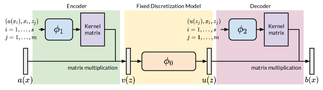
Figure 3: Models of the nonlinear integral transforms in the 3-component structure of a one-layer IAE. The encoder implements the nonlinear integral transform in Equation (8) using matrix multiplication, using $\phi_{1}$ to build the kernel matrix (blue dashed box). The decoder implements the nonlinear integral transform in Equation (9), using $\phi_{2}$ to build the kernel matrix (blue dashed box). $\phi_{0}$ is an FNN described in Section 2.3.1. The kernel matrix represents the matrix $K$ (see Equation (5)) with $i,j$-entries $\phi_{1}(a(x_{i}),x_{i},z_{j})$ and $\phi_{2}(u(z_{i}),x_{j},z_{i})$ respectively for the encoder and decoder.

Equations (8) and (9) can be composed repeatedly using multiple $\phi_{1}$ and $\phi_{2}$, respectively, into an $N$-layer IAE, where $N$ represents the number of compositions. Let $\phi_{1}^{1}(\cdot;\theta_{\phi_{1}^{1}}),$ $\dots,$ $\phi_{1}^{N}(\cdot;\theta_{\phi_{1}^{N}})$ denote $N$ nonlinear integral kernels. The mapping from $a$ to $v$ is implemented recursively as follows. In the $i$-th layer, for $i=1,\dots,N$, a nonlinear integral transform is performed via

$$v_{i}(z)=\int_{\Omega_{v_{i-1}}}\phi_{1}^{i}(v_{i-1}(x),x,z;\theta_{\phi_{1}^{i}})v_{i-1}(x)dx,\quad z\in\Omega_{v_{i}},$$ (10)

where $v_{0}:=a$, $v_{i}$ is defined on $\Omega_{v_{i}}$ for $i=0,\dots,N$. $v_{N}$ is denoted as $v$, thus the mapping from $a$ to $v$ follows $a\rightarrow v_{1}\rightarrow\dots\rightarrow v_{N}=v$. Similarly, let $\phi_{2}^{1}(\cdot;\theta_{\phi_{2}^{1}}),\dots,\phi_{2}^{N}(\cdot;\theta_{\phi_{2}^{N}})$ denote $N$ nonlinear integral kernels. The mapping from $u$ to $b$ is also performed recursively, such that in the $i$-th layer, where $i=1,\dots,N$, a nonlinear integral transform is performed, given by

$$u_{i}(x)=\int_{\Omega_{u_{i-1}}}\phi_{2}^{i}(u_{i-1}(z),x,z;\theta_{\phi_{2}^{i}})u_{i-1}(z)dz,\quad x\in\Omega_{u_{i}},$$ (11)

where $u_{0}:=u$, $u_{i}$ is defined on $\Omega_{u_{i}}$ for $i=0,\dots,N$. $u_{N}$ is denoted as $b$, thus the mapping from $u$ to $b$ follows $u\rightarrow u_{1}\rightarrow\dots\rightarrow u_{N}=b$. The spaces $\Omega_{v_{i}}$, for $i=1,\dots,N$, and $\Omega_{u_{j}}$, for $j=0,\dots,N-1$, as well as their corresponding set of grid points, are chosen by the user. The set of grid points $S_{z}$ of $\Omega_{v_{N}}=\Omega_{u_{0}}=\Omega_{z}$ is chosen to be fixed and, hence, is independent of any set of grid points $S$ of $\Omega$. This allows the mapping from $v$ to $u$ to be implemented using a fixed-size FNN $\phi_{0}$. Aside from the integral kernels $\phi_{i}^{j}$, for $i=1,2$ and $j=1,\dots,N$, no other FNN is present in the implementation of the nonlinear integral transforms. These nonlinear integral kernels in Equations (10) and (11) only require pointwise information as inputs, thus they do not depend on how the input function is discretized. Hence, except for $\Omega_{v_{N}}$ and $\Omega_{u_{0}}$, the number of grid points for the other intermediate spaces are allowed to depend on $s$, the number of grid points from $\Omega$ used to discretize $a$ and $b$.

The final mapping, using $\phi_{1}^{i}(\cdot;\theta_{\phi_{1}^{i}})$, for $i=1,\dots,N$, to build the composite mapping from $a$ to $v$, $\phi_{2}^{j}(\cdot;\theta_{\phi_{2}^{j}})$, for $j=1,\dots,N$, to build the mapping from $u$ to $b$, and $\phi_{0}$ to map $v$ to $u$, forms an $N$-layer IAE. The objective of composing multiple integral transforms is to learn a feature-rich representation of the data, analogous to the multilayer MLP and FNNs. For simplicity of notation, for the rest of the paper, unless otherwise stated, we refer to the integral kernels of an IAE by considering a $1$-layer IAE, i.e., $\phi_{1}$ (Equation (8)) and $\phi_{2}$ (Equation (9)) denotes the integral kernels of an IAE.

2.3.2 Multi-Channel Learning

Instead of using the original function as the input and output of IAE (defined in Section 2.3.1), it is typically beneficial to process information in a transformed domain, where the original information admits sparsity after transformation. This is useful to capture various phenomena emphasized in other domains. For example, oscillatory phenomena, commonly found in problems like signal processing, are better represented in the Fourier domain, where highly oscillatory information is found in the higher frequency bands, and the lower frequency data are well separated from the higher frequency data. In IAE-Net, we propose a multi-channel learning framework, denoted as IAE blocks, or $\mathcal{IAE}(\cdot;\theta_{\mathcal{IAE}})$, to allow IAE-Net to solve a wider range of problems. Here $\theta_{\mathcal{IAE}}$ denotes the parameters of this block.

In this multi-channel learning framework, IAEs are applied in parallel, where in addition to the original input function, alternative branches are applied to transformed inputs using known integral transforms like the Fourier or Wavelet Transform. A $c$-channel IAE block is constructed by first denoting $\mathcal{F}_{1},\dots,\mathcal{F}_{c-1}$ as $c-1$ integral transforms, together with their corresponding inverses $\mathcal{F}^{-1}_{1},\dots,\mathcal{F}^{-1}_{c-1}$. These integral transforms map the input function $a$ to another transformed domain. The transformed functions $\mathcal{F}_{i}a$, $i=1,\dots,c-1$, together with $a$, become $c$ different inputs used for each of the branches (see Figure 2 for a visualization). These functions are used to implement a $c$-channel IAE block via

$$\mathcal{IAE}(a;\theta_{\mathcal{IAE}}):=M([\Phi_{1}(a;\theta_{\Phi_{1}}),\mathcal{F}^{-1}_{1}\Phi_{2}(\mathcal{F}_{1}a;\theta_{\Phi_{2}}),\dots,\mathcal{F}^{-1}_{c-1}\Phi_{c}(\mathcal{F}_{c-1}a;\theta_{\Phi_{c}})];\theta_{M}),$$ (12)

where $[\cdot,\dots,\cdot]$ denotes the concatenation operator along the channel axis; $\Phi_{i}$, for $i=1,\dots,c$, represents the $i$-th IAE; and $M(\cdot;\theta_{M})$ parametrized by $\theta_{M}$ is a pointwise MLP (see Equation (2)) post-processing and merging the outputs of each channel. Figure 2 shows a $2$-channel IAE block designed using the original input and the Fourier transform. Appendix A.2 and A.3 provides additional numerical experiments motivating the choice of using a multi-channel learning framework and a channel MLP for post processing.

2.3.3 Densely Connected Multi-Block Structure

The IAE blocks defined in Section 2.3.2 are composed repeatedly with pointwise linear transforms of the outputs from previous IAE blocks to form a densely connected multi-block structure motivated by DenseNet [72]. This follows the computational flow introduced in Section 2.3 and will be proposed as the final IAE-Net, denoted as $\Psi^{n}(\cdot;\theta_{\Psi^{n}})$. Here, $\theta_{\Psi^{n}}$ denotes the parameters of $\Psi^{n}$.

The composition of the blocks in IAE-Net is formulated as follows. Consider the $i$-th IAE block in a $L$-block IAE-Net, denoted by $\mathcal{IAE}_{i}(\cdot;\theta_{\mathcal{IAE}_{i}})$, where $i=1,\dots,L$. In addition, $\mathcal{A}_{j}(\cdot;\theta_{\mathcal{A}_{j}})$ is defined as pointwise affine transforms parametrized by $\theta_{\mathcal{A}_{j}}$, taking in $a_{j}$ as its input, for $j=0,\dots,L-1$. Then, this composition is performed with skip connections from all the preceding outputs $a_{0},\dots,a_{i-1}$ via

$$a_{i}=\sigma(\mathcal{IAE}_{i}(\mathcal{M}_{i}([\mathcal{A}_{0}(a_{0};\theta_{\mathcal{A}_{0}}),\mathcal{A}_{1}(a_{1};\theta_{\mathcal{A}_{1}}),\dots,\mathcal{A}_{i-1}(a_{i-1};\theta_{\mathcal{A}_{i-1}})];\theta_{\mathcal{M}_{i}});\theta_{\mathcal{IAE}_{i}})),$$ (13)

where $[\cdot,\dots,\cdot]$ denotes the concatenation operator along the channel axis; $\mathcal{M}_{j}(\cdot;\theta_{\mathcal{M}_{j}})$ parametrized by $\theta_{\mathcal{M}_{j}}$ is a pointwise MLP (see Equation (2)) merging the outputs of each of the linear transformed outputs from the previous IAE blocks; and $\sigma$ is an activation function. The resulting IAE-Net is visualized in Figure 4.

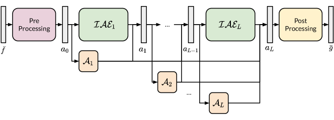
Figure 4: Structure of a $L$ block IAE-Net. For $i=1,\dots,L$, $\mathcal{IAE}_{i}$ represents IAE blocks, described in Equation (12), $\mathcal{A}_{i}$ refers to the pointwise linear transforms implemented in a densely connected structure in Equation (13), and the pre and post processing block is built with $F$ and $G$ described in Section 2.3. The numerical implementation of all the components are described in Section 3.2.

This densely connected structure diversifies the features of the inputs to each IAE block, allowing IAE-Net to learn complex representations of the data. In addition, it helps to lessen the gradient vanishing issue commonly observed in FNNs [73], thus providing additional stability to IAE-Net. This is shown through extensive experiments in Section 3, where IAE-Net achieves consistent performance better than numerous other deep NN structures in a wide range of applications. Appendix A.1 presents numerical experiments to show that the performance of IAE-Net is almost improved by $100\%$ as compared to using a single block.

2.3.4 Data Driven Discretization Invariant Learning

Let $\Psi^{n}(\cdot;\theta_{\Psi^{n}})$ denote the proposed IAE-Net parametrized by $\theta_{\Psi^{n}}$ (defined in Section 2.3.3). For simplicity, we assume that $\Psi^{n}$ is built using $1$-layer IAEs within each IAE block, so $\phi_{1}(\cdot;\theta_{\phi_{1}})$ (see Equation (8)) and $\phi_{2}(\cdot;\theta_{\phi_{2}})$ (see Equation (9)) refers to the integral kernels used in a $1$-layer IAE located in $\Psi^{n}$, where $\theta_{\phi_{1}}$ and $\theta_{\phi_{2}}$ parametrize $\phi_{1}$ and $\phi_{2}$ respectively. Given that these integral kernels are modelled as NNs, their performance depends on the given data. Take, for example, a data set consisting of data sampled from a specific set of grid points $S$ in $\Omega$. During training, $\phi_{1}$ and $\phi_{2}$ are only trained to output suitable kernel values for the grid points in $S$. The performance of these kernels deteriorates when tested on other grid points not found in $S$. Thus, being data-driven, $\phi_{1}$ and $\phi_{2}$ suffer from poor generalization errors. To reduce this error, this paper proposes a novel data augmentation procedure to exploit the discretization invariant structure of IAE-Net. The procedure involves augmenting the training process with different resolutions of the data, obtained via interpolation of the given data. This method promotes the learning of $\phi_{1}$ and $\phi_{2}$, allowing them to output suitable kernel values from inputs of various sizes.

Let $\mathcal{X}$ denote a function space of functions defined on $\Omega$, and define $X_{S}=\{\bar{f}|f\in\mathcal{X}\}$ as the set of numerical observations $\bar{f}$ of functions $f\in\mathcal{X}$ sampled using grid points in $S\subset\Omega$. Typically, during training, the available training data are sampled from $X_{S}$. Let $\mathcal{S}$ denote the set of all possible non-empty finite subsets of $\Omega$. i.e., $S\subset\mathcal{S}$ represents a set of grid points from $\Omega$. Given observations of a problem sampled from grid points $S\in\mathcal{S}$, and $T\in\mathcal{S}$ another set of grid points of $\Omega$, an interpolator function $I_{T}:X_{S}\rightarrow X_{T}$ maps numerical observations $\bar{f}\in X_{S}$ to numerical observations $I_{T}(\bar{f})\in X_{T}$ sampled (using grid points in $T$) from the interpolant $l\in\mathcal{X}$ obtained from $\bar{f}$. By definition, an interpolant $l\in\mathcal{X}$ of $f$ from observations $\bar{f}\in X_{S}$ is a function approximating $f$ that agrees with $f$ on the set of points in $S$, i.e., $\bar{l}=\bar{f}$. Typical examples of interpolants are linear, bilinear, and cubic spline interpolation.

Define $\mathcal{I}:=\{I_{T}|T\in\mathcal{S}\}$ as the set of all such interpolator functions. At each iteration of the SGD when training IAE-Net, the training samples are augmented with the interpolations of the data using $I_{T}\in\mathcal{I}$, i.e., we optimize the following objective function via SGD:

$$\min_{\theta_{\Psi^{n}}}\mathbb{E}_{(\bar{f},\bar{g})\sim p_{data}}\mathbb{E}_{I_{T}\sim\mathcal{I}}[L(\Psi^{n}(\bar{f};\theta_{\Psi^{n}}),\bar{g})+\lambda L(\Psi^{n}(I_{T}(\bar{f});\theta_{\Psi^{n}}),I_{T}(\bar{g}))],$$ (14)

where $\lambda$ is a hyperparameter, $p_{data}$ is the distribution of the training data pair $(\bar{f},\bar{g})$, and $\Psi^{n}(\cdot;\theta_{\Psi^{n}})$ denotes the proposed IAE-Net parameterized by $\theta_{\Psi^{n}}$. Equation (14) leverages the discretization invariance of IAE-Net to train the integral kernels of each IAE within $\Psi^{n}$ with inputs of varying discretizations. This is crucial to allow IAE-Net to achieve discretization invariance even with data-driven kernels. Usually, $\mathcal{S}$ contains an infinite number of discretization formats. So in practice, only a finite subset $U\subset\mathcal{S}$ of commonly used discretization formats is considered.

3 Numerical Experiments

In this section, we present the experimental results comparing the performance of IAE-Net in a wide range of applications.

3.1 Baseline Models

The performance evaluation of IAE-Net is compared against the following baseline models.

1. ResNet+Interpolation implements a naive method to achieve discretization invariance for fixed-discretization models. Interpolation is a simple and commonly used method for heterogeneous data structures traditionally in the literature. This method is implemented with an interpolation function interpolating the data from any arbitrary discretization to a fixed discretization $\Omega$ for input to the NN. The output performs interpolation back to $\Omega$. For this baseline, a ResNet [73] is adopted with similar number of parameters to IAE-Net as the fixed-discretization model.

2. Unet [17] is a popular tool for signal separation tasks. Although the fully convolutional structure allows Unet to take inputs sampled using different discretization formats, the model is usually used with a fixed discretization format of the input space. This is because the convolutional layers in Unet perform local processing of the inputs using a small kernel, which makes it difficult to adapt to varying input scales. This can be seen in the numerical experiments, where the performance of Unet collapses significantly when applied naively to other resolutions.

3. DeepONet [23, 24] is proposed as an operator learner which is semi-discretization invariant. The original model, although discretization invariant to the output, is however not discretization invariant to the inputs, where a fixed discretization is used to learn an encoding of the input function.

4. Fourier Neural Operator (FNO) [14] is proposed as a seminal discretization invariant operator learner on numerous mathematically well-posed benchmark data sets.

5. Fourier Transformer (FT), Galerkin Transformer (GT) [15] are proposed as discretization invariant operators applying transformer encoders to encode given data [3] and the blocks in [14] for post-processing. The model achieves state-of-the-art performance in its benchmark data sets.

The original code provided by the authors is referenced for all the baselines, obtained from their Github pages. For the experiments, their choice of settings for the hyperparameters and training procedures are used (e.g., modes, width in FNO, and initialization for attention matrices in FT, GT) to train their models. Since DeepONet is not discretization invariant to the input data, to obtain results for different resolutions, the models are separately trained using different resolutions. Similarly, Unet requires repeated training when test data have different resolutions. In the next section, the numerical setup of the experiments will be provided in detail. Following this, the remainder of Section 3 will show the numerical experiments of IAE-Net and the above baselines in a wide range of problems. We will numerically demonstrate the following conclusions:

• Naive interpolation-based method with a fixed-size neural network, FNO, GT/FT, and IAE-Net can achieve zero/few shot generalization in well-posed problems like solving parametric PDEs and initial value problems.

• Existing methods fail to provide zero/few shot generalization in ill-posed problems and/or for highly oscillatory data, while IAE-Net succeeds to generalize well.

• IAE-Net outperforms all existing baseline methods with better accuracy in all test examples.

3.2 Training Details

For all applications, grid points are sampled using a uniform grid in $[0,1]^{d}$, where $d$ represents the dimension of the problem. Let $S_{1}\subset[0,1]$ and $S_{2}\subset[0,1]^{2}$, denote the set of grid sizes used to discretize the input and output functions for the $1$-d and $2$-d problem respectively. For $1$-d problems, i.e., $d=d_{x}=d_{y}=1$, a uniform grid sampled from $[0,1]$ is used. That is, $S_{1}=\{\frac{i-1}{s-1}\}^{s}_{i=1}$ where $s$ denotes the discretization size, which is not fixed. For the fixed $S_{z}$ containing the grid points for discretizing the intermediate function $u$ and $v$ in IAE (see Section 2.3.1), we set $m=256$, where $m$ denotes the discretization size, thus $S_{z}=\{\frac{i-1}{255}\}^{m}_{i=1}$. For the $2$-d problem, i.e., $d=d_{x}=d_{y}=2$, a $2$-d uniform mesh is used, such that $S_{2}=S_{1}\times S_{1}=\{(\frac{i-1}{s-1},\frac{j-1}{s-1})\}$, with $\times$ representing the cartesian product, and $i,j=1,\dots,s$ where $s$ denotes the discretization size along one axis. For $S_{z}$ in the $2$-d problem, we set $m=64$, where $m$ denotes the discretization size along one axis, thus $S_{z}=\{(\frac{i-1}{63},\frac{j-1}{63})\}$, with $i,j=1,\dots,64$.

The recursive architecture in IAE-Net is constructed by stacking four $\mathcal{IAE}$’s in the densely connected structure described in Equation (13), with the ReLU activation function as $\sigma$, and a single hidden layer pointwise MLP for $\mathcal{M}$. Thus $L=4$ in the experiments. The pointwise affine transform $\mathcal{A}$ in Equation (13) is implemented using pointwise linear transforms. Each $\mathcal{IAE}$ is constructed following Equation (12), using a $2$-channel IAE block taking in the original input and the Fourier transformed input for each of the respective channels, visualized in Figure 2.

For the $1$-d case, a $1$-layer IAE is used, while a $2$-layer IAE is used in the $2$-d case. For the nonlinear integral transforms $\phi_{1}^{1}$ and $\phi_{1}^{2}$ (Equation (10)) in the $2$-layer IAE, $\phi_{1}^{1}$ is used to first map $S_{2}$ to $S_{f}=\{(\frac{i-1}{63},\frac{j-1}{s-1})\}$, where $i=1,\dots,m$ and $j=1,\dots,s$ before mapping to $S_{z}$ using $\phi_{1}^{2}$, following Equation (10). This can be understood as performing an integral transform on the $x$-axis, followed by the $y$-axis. For the nonlinear transforms $\phi_{2}^{1}$ and $\phi_{2}^{2}$, $\phi_{2}^{1}$ is used to first map $S_{z}$ to $S_{f}$, before mapping to $S_{2}$ using $\phi_{2}^{2}$, following Equation (11). A single hidden layer FNN is used to design $\phi_{1}$ and $\phi_{2}$ in the $1$-d case, as well as $\phi_{1}^{1}$, $\phi_{1}^{2}$, $\phi_{2}^{1}$ and $\phi_{2}^{2}$ in the $2$-d case. A single hidden layer pointwise MLP is applied to the outputs of the nonlinear integral transforms. A two hidden layer FNN is used for $\phi_{0}$ in both cases. $M$ (see Equation (12)) is implemented using a single hidden layer pointwise MLP. As defined in Section 2.3, pre processing is done using a pointwise linear transform $F$ mapping the input observations $\bar{f}$ to $\mathbb{R}^{w}$, where $w$ denotes the length of the projected vector. Post processing is done using two FNO blocks followed by a pointwise linear transform, following $G$ in Section 2.3 mapping $a_{L}$ to $\bar{g}$. We set $w=64$ for both the $1$-d and $2$-d problems. Figure 4 shows the structure of IAE-Net.

The data augmentation (DA) strategy proposed in Equation (14) is used by default for IAE-Net, with $\lambda=1$, using interpolation of the training data to the testing sizes. Lower resolution data representing $I_{T}(\bar{f})$ and $I_{T}(\bar{g})$ are obtained by downsampling from a higher resolution, while higher resolution data are obtained with cubic and bicubic interpolation for the $1$-d and $2$-d problems respectively. IAE-Net is trained for all the applications with a learning rate of $0.001$, using Adam optimizer as the choice of optimizer. A batch size of 50 for $1$-d problems, and 5 for $2$-d problems, is used, and training is performed for 500 epochs using a learning rate scheduler scaling the learning rate by $0.5$ on a plateau with patience of $20$ epochs. All the models are trained using the $L2$ relative error, denoted as $\mathcal{L(\cdot,\cdot)}$, as the loss function, defined by

$$\mathcal{L}(x,y):=\frac{||x-y||^{2}}{||y||^{2}}.$$ (15)

The performance of all the models will also be evaluated using the mean $L2$ relative error, defined in the above Equation (15). The experiments are run with a 48GB Quadro RTX 8000 GPU.

Alternative architectures for IAE-Net are considered for additional baselines. The first adopts the ResNet [73] style skip connection performing an elementwise summation of the skip connection with the output of the IAE-Net block. For this baseline, instead of Equation (13), the output for the $i$-th IAE block is defined as

$$f_{i}=\sigma(\mathcal{IAE}_{i}(f_{i-1})+\mathcal{A}_{i}(f_{i-1})),$$ (16)

with $\sigma$ as the ReLU activation, and $\mathcal{A}_{i}$ as a pointwise linear transform. The second is a base model without any skip connections between the blocks. These baselines evaluate the performance of IAE-Net with varied forms of skip connections and motivates our choice of using the densely connected structure in the proposed IAE-Net. The two models are denoted IAE-Net (ResNet) and IAE-Net (No Skip) respectively.

3.3 Predictive Modelling

The first application lies in the solving of predictive modelling problems. For this problem, the Burgers Equation is considered, given by

$$\begin{split}\partial_{t}u(x,t)+\partial_{x}(u^{2}(x,t)/2)&=\nu\partial_{xx}u(x,t),\quad x\in(0,1),t\in(0,1]\\ u(x,0)&=u_{0}(x).\end{split}$$ (17)

with periodic boundary conditions. In this application, the objective is to learn the mapping from an initial state/condition $u_{0}$ to the solution $u$ at time $t=1$. That is, the operator to be learnt is $\Psi$ mapping $u_{0}(.,0)\rightarrow u(.,1)$ for $x\in(0,1)$. Here, $\nu$ represents the viscosity of the problem. This problem is used as one of the benchmark problems in [14, 15].

The initial conditions to generate this data set, provided by [14] in https://github.com/zongyi-li/fourier_neural_operator, is generated according to $u_{0}\sim\mu$, where $\mu=\mathcal{N}(0,\sigma^{2}(-\Delta+\tau^{2}I)^{-\alpha})$, using $\tau=5$, $\sigma=\tau^{2}$ and $\alpha=2$. Viscosity is set to $\nu=0.1$, and the equation is solved via a split step method where the heat equation component is solved exactly in the Fourier space and the non-linear part is advanced in the Fourier space, using a fine forward Euler method. A total of 10000 training samples and 1000 testing samples are generated.

For the experiments, the length $s=1024$ data is used to train IAE-Net, FNO, FT, GT and ResNet+Interpolation, and the resulting trained model is tested on resolutions $s=256,512,1024,2048,8192$. For DeepONet, due to the input being non-discretization invariant, the model is trained separately on the different resolutions. Due to out-of-memory issues when loading the DeepONet data set for larger resolutions, the results for those resolutions are omitted. This particular issue highlights the drawback of non-discretization invariant models: These models require expensive re-training to train a new NN for different discretization formats, often which, the computational costs to train the model for large resolution data is extremely high. The results for this data set are shown in Figure 5.

Figure 5: $L2$ relative error (Equation (15)) on the burgers data set with $\nu=1e^{-1}$ (Left) and its closeup (Right). Models are trained with $s=1024$ and tested on the other resolutions.

In this data set, IAE-Net performs almost 3 times better than FNO, FT, and GT, while significantly outperforming both DeepONet and ResNet+Interpolation. Comparing the results of IAE-Net (No Skip) and IAE-Net (ResNet) with IAE-Net, the use of a densely connected structure significantly improves the capability of the model, performing almost 2 times better than the ResNet counterpart. This comes at minimal cost to the evaluation speed of the network, which is compared in Appendix B. The effect of the proposed data augmentation method is seen by comparing the results of IAE-Net (No DA) to IAE-Net. In the former, IAE-Net (No DA) achieves good performance only on the resolution it is trained on, but the model does not perform well on other resolutions. In the latter, the use of data augmentation leads to consistent test error across the different resolutions. This supports the use of the proposed data augmentation, as the data reliant IAE kernels require training on different resolution scales to learn heterogeneous structures across resolutions.

Next, we explore the effects of viscosity on model performance. A data set of 1000 training data and 100 testing data is generated with $\nu=1e^{-4}$ and tested with IAE-Net, FNO, FT, GT, and DeepONet. The results for $\nu=1e^{-4}$ is shown in Figure 6. IAE-Net achieves the best performance compared to the other baselines. Further experiments are conducted to test the performance of IAE-Net, FNO and GT for varying degrees of $\nu$, using 1000 training and 100 testing data for each $\nu=1e^{-4},1e^{-3},1e^{-2},1e^{-1}$ and $1$. The results comparing the performance of the models across different viscosities and the relative error ratio comparing the errors of FNO and GT against IAE-Net at each $\nu$ are shown in Figure 7. This ratio is computed using $\frac{m_{e}-i_{e}}{i_{e}}$, where the $L2$ relative error of FNO or GT is denoted by $m_{e}$ and the $L2$ relative error of IAE-Net is denoted by $i_{e}$.

Figure 6: $L2$ relative error (Equation (15)) on the burgers data set with $\nu=1e^{-4}$ (Left) and its closeup (Right). The closeup of the figure is shown on the right. Models are trained with $s=1024$ and tested on the other resolutions.

Figure 7: Comparison of relative error (Equation (15)) for burgers equation with varying $\nu$ (Left) and the relative error ratio comparing the relative errors of FNO and GT against IAE-Net at each $\nu$ (Right). Models are trained with $s=1024$, and tested with $s=1024$ testing data.

IAE-Net outperforms FNO and GT on all viscosities, demonstrating the generalization capability of the model. In contrast, we observe varied performance in FNO and GT. For $\nu=1$, GT fails to achieve good results. On the other viscosities, it can be seen that the performance of FNO starts to deviate from IAE-Net as $\nu$ increases to $0.1$, while the performance of GT deviates from IAE-Net as $\nu$ decreases to $0.0001$. Due to the focus of these methods on well-posed problems, the performance of these baselines starts to deviate when applied to the same problem, but under different well-posedness conditions.

Next, we conduct an experiment to test IAE-Net on inputs with a non-uniform grid. IAE-Net is trained and tested on the Burgers equation data set with viscosity $\nu=1e^{-1}$. The non-uniform grids are obtained via randomly subsampling $s=256,512,1024,2048,4096$ sorted points from the size $s=8192$ data. The subsampling is done such that the end-points $x=0$ and $x=1$ are always included, to ensure that the boundary condition is satisfied. The performance of IAE-Net is compared against DeepONet and ResNet+Interpolation, two baseline models that can handle non-uniform grids. Due to out-of-memory issues when loading the DeepONet data set for larger resolutions, the results for those resolutions are omitted. The results are shown under Figure 8. IAE-Net achieves the lowest $L2$ relative error as compared to the other baselines, showing how IAE-Net can also be applied to non-uniform grids.

Figure 8: $L2$ relative error (Equation 15) on the Burgers data set with non-uniform grid. ResNet+Interpolation and IAE-Net are trained with randomly subsampled sorted points of sizes $s=256,512,1024,2048,4096$ and tested on the same resolutions. As DeepONet is not discretization invariant to the inputs, a separate training is performed for each resolution.

3.4 Forward and Inverse Problems

IAE-Net is evaluated on two Forward and Inverse Problems.

3.4.1 Darcy Flow

IAE-Net is demonstrated on the forward problem solving the Darcy flow equation. The Darcy flow equation is given by

$$\begin{split}-\nabla\cdot(a(x)\nabla u(x))&=f(x),\quad x\in(0,1)^{2}\\ u(x)&=0,\quad x\in\partial(0,1)^{2},\end{split}$$ (18)

with a Dirichlet boundary condition, with $a$ as the diffusion coefficient and $f$ the forcing function. In this problem, the forward problem is defined as the mapping from the diffusion coefficient $a$ to the solution $u$, i.e., $a(\cdot)\rightarrow u(\cdot)$ for $x\in(0,1)^{2}$. The Darcy Flow is used as the 2D benchmark problem in [14, 15], and also explored in works like [20].

In the benchmark data set, the coefficients $a(x)$ are generated according to $a\sim\mu$ where $\mu=\psi(\mathcal{N}(0,(-\Delta+\tau^{2}I)^{-\alpha}))$, $\tau=3$ and $\alpha=2$ with zero Neumann boundary conditions on the Laplacian. The mapping $\psi:\mathbb{R}\rightarrow\mathbb{R}$ takes the value 12 on the positive part of the real line and 3 on the negative, and the forcing function is taken to be $f(x)=1$. The solutions $u$ are obtained using a second-order finite difference scheme. The code to generate the data set is provided by [14] in https://github.com/zongyi-li/fourier_neural_operator. A total of 1000 training data and 100 testing data obtained from the benchmark data set is used for the experiment.

The models are trained with $s=141$ training data and tested on testing data for each of the resolutions $s=85,106,141,211$. The results are shown in Figure 9. In this baseline, IAE-Net outperforms all baselines, achieving state-of-the-art error. In this problem, it can be seen that the use of ResNet skip connections in IAE-Net (ResNet) does not perform well. One possible explanation is the difference in the structure of $a$, a piecewise constant function, with $u$, which is smooth, thus the residuals from the ResNet skip connection may not be as important to producing the final output $u$. Surprisingly, it was observed that the performance of the ResNet+Interpolation model performs better than FNO, FT, and GT. This observation suggests that data-driven learning may provide additional benefits to the overall performance, by learning key data-driven features, in this problem. Thus, IAE-Net, which contains the data-driven IAE kernels, is able to outperform existing discretization invariant methods in this application.

Figure 9: $L2$ relative error (Equation (15)) on the benchmark darcy data set. Models are trained with $s=141$ size training data and tested on the other resolutions.

Next, the performance of IAE-Net is tested on the Darcy problem in a triangular domain with a notch [81]. This experiment evaluates the performance of IAE-Net when applied to general domains. Following the Darcy flow equation (Equation 18) with $a(x)=0.1$ and $f=-1$, the operator to be learnt is the mapping from the boundary values $u(x)|_{\partial\Omega}\rightarrow u(x)$, where $\Omega$ is defined as a 2D triangular domain where the corners are given by the following coordinates: $(0,0)$, $(1,0)$ and $(\frac{1}{2},\frac{\sqrt{3}}{2})$, with a rectangular notch where the corners are given by the following coordinates: $(0.49,0)$, $(0.51,0)$, $(0.51,0.4)$ and $(0.49,0.4)$, where $x\in\Omega$. Each boundary of the triangular domain in $\Omega$ is a function $h(y)$, where $y\in[0,1]$, generated via a Gaussian process $\mathcal{GP}$ given by

$$\begin{split}h(y)&\sim\mathcal{GP}(0,\mathcal{K}(y,y^{\prime})),\\ \mathcal{K}(y,y^{\prime})&=\exp[-\frac{(y-y^{\prime})^{2}}{2l^{2}}],\quad l=0.2,\\ y,y^{\prime}&\in[0,1],\end{split}$$ (19)

while the boundary values at the boundaries of the notch are fixed as $h(x)=1$. The ground truth is simulated using the PDE Toolbox in Matlab [82].

IAE-Net is trained following the data set provided for FNO training by the original paper [81] in https://github.com/lu-group/deeponet-fno, which consists of 2000 samples, of which 1900 samples are used as training data and 100 samples are used as test data. IAE-Net is compared against 3 models found in [81]: DeepONet [23, 24], POD-DeepONet [81] which replaces the trunk net in DeepONet with a proper orthogonal decomposition (POD) on the training data, and dgFNO+ [81], which extends FNO [14] to a general domain. Due to out-of-memory issues when loading the DeepONet and POD-DeepONet data set for larger resolutions, the results for those resolutions are omitted. The $L2$ relative error (see Equation 15) is shown in Table 2. In this application, IAE-Net achieves the lowest $L2$ relative error compared to the other baselines.

Table 2: Results on the Darcy problem in a triangular domain with a notch. IAE-Net is trained with $s=50$ data, and tested on $s=50,100,200$ resolutions. Errors are the $L2$ relative error described in Equation (15), scaled by $1e^{2}$ to show percentage error. Results labelled with ^∗ are obtained from [81].

Model Name	50	100	200
$DeepONet^{*}$	2.64%
$POD-DeepONet^{*}$	1.00%
$dgFNO+$	7.821%	7.819%	7.822%
IAE-Net	0.8094%	0.8136%	0.8317%

3.4.2 Scattering Problem

The inhomogeneous media scattering problem [52] with a fixed frequency $\omega$ is modelled by the Helmholtz operator

$$Lu:=(-\Delta-\frac{\omega^{2}}{c^{2}(x)})u,$$ (20)

where $c(x)$ is the velocity field. In most settings, a known background velocity field $c_{0}(x)$ exists, such that except for a compact domain $\Omega$, $c(x)$ is identical to $c_{0}(x)$. Thus, by introducing a scatterer $\eta(x)$ that is compactly supported in $\Omega$, i.e.,

$$\frac{\omega^{2}}{c(x)^{2}}=\frac{\omega^{2}}{c_{0}(x)^{2}}+\eta(x),$$ (21)

then it is possible to work equivalently with $\eta(x)$ instead of $c(x)$. In real-world applications, observation data $d(\cdot)$, derived from the Green’s function $G=L^{-1}$ of the Helmholtz operator $L$, is used to evaluate $\eta(\cdot)$. In this field, both the forward map $\eta\rightarrow d$ and the inverse map $d\rightarrow\eta$ are useful for their numerical solutions of the scattering problems. The former provides an alternative to expensive numerical PDE solvers for the Helmholtz equation, while the latter allows one to determine the scatterers from the scattering field, without the usual iterative procedure. The data set is obtained from [52].

For the scattering problem, the model is trained with 10000 $s=81$ training data and tested on 1000 testing data for each of the resolutions $s=27,41,81,161,241$ for both the forward and inverse problems. The data is generated using $\omega=18\pi$. The results are shown in Figure 10. IAE-Net succeeds in this application while FNO, FT, and GT fail in this case, achieving more than 10 times higher error than IAE-Net. In this application, it was also observed that the performance of ResNet+Interpolation model performs better than FNO, FT, and GT. Similar to the Darcy problem, this suggests the benefits of including data-driven learning via the use of IAE in IAE-Net, which helped to improve the performance of the model, allowing IAE-Net to achieve the best performance.

Figure 10: $L2$ relative error (Equation (15)) on the scattering data set for the forward (Left) and inverse (Right) problem. Model is trained with $s=81$ and tested on different resolutions.

In addition, all the baseline models show signs of deterioration in resolutions away from the trained resolution $s=81$. Using the proposed data augmentation, this error is alleviated in IAE-Net. In this case, where the problem becomes ill-posed, the performance of models like FNO, FT, and GT which focus on mathematically well-posed problems start to fall off. Including data augmentation in IAE-Net allows the model to capture features on different scales, while the use of data-driven IAE helps to learn suitable features in the data set, thus leading to consistent performance.

As mentioned in the introduction, aside from the application of IAE-Net to zero-shot learning, an additional experiment is conducted to explore the application of IAE-Net to one more situation: data sets from multiple resolutions are used to perform training. For this experiment, a combined data set is assembled consisting of 10000 data points generated independently for each of the resolutions $s=81,108,162$, forming a combined total of 30000 data. The data is generated using $\omega=18\pi$. Training is done without resizing the data. As existing deep learning software like Pytorch and Tensorflow do not support batching of data with different resolutions in one batch, additional methods to batch the data need to be considered. Here, two different methods of training are considered: 1) Each data set is loaded sequentially and trained for $10$ epochs before loading the next data set. This model is denoted as IAE-Net (Sequential). 2) In each epoch, a random batch of data is loaded from each resolution, and each batch is passed separately into the model. The losses computed for each batch are summed for backpropagation. The results are shown in Figure 11. We observe that IAE-Net (Sequential) performs poorly, where the model does not converge well, whereas the second method shows better performance, reaching good test error in IAE-Net.

Figure 11: $L2$ relative error (Equation (15)) on the scattering data set using different data generated with different resolutions. Each resolution consists of 10000 data generated independently from each other, forming a combined total of 30000 data. Sequential training is performend by training the model through loading the data sets in sequence. The last data set in the sequential training is the size $s=162$ data set.

3.5 Image Processing

For image processing, IAE-Net is applied to solve a denoising problem. In medical computed tomography (CT) imaging problems, an interesting application is to learn the reconstruction of phantom images from the corresponding filtered backprojection (FBP) CT images with noise added to the projections [19]. In this application, the projections are expressed in terms of the ray transform $\mathcal{P}:\mathcal{X}\rightarrow\mathcal{Y}$, where $\mathcal{X}$ represents the image function space, and $\mathcal{Y}$ is the measurement function space with $\mathcal{P}$ given by

$$\mathcal{P}(f)(l)=\int_{l}f(x)dx,\quad l\in\mathbb{M},$$ (22)

where $l$ are lines from an acquisition geometry $\mathbb{M}$. The inverse operator $\mathcal{P}^{-1}$ is of practical importance, as it allows us to reconstruct the unknown density $f\in\mathcal{X}$ from it’s known attenuation data $\mathcal{P}(f)$. This inverse problem is ill-posed, that is, given attenuation data $\mathcal{P}(f)$, suppose a solution $f$ to the inverse problem exists, it is unstable with respect to $\mathcal{P}(f)$, where small changes to $\mathcal{P}(f)$ results in large changes to the reconstruction. Thus, the impact of noise added to the projections makes the problem difficult to solve, and solving the problem directly typically leads to over-fitting against the projection data. A solution is to consider a knowledge-driven reconstruction. That is, instead of learning the direct inverse $\mathcal{P}^{-1}$ using an NN, a knowledge-driven component $\mathcal{A}:\mathcal{Y}\rightarrow\mathcal{X}$ is considered and the inverse is learned using

$$\mathcal{P}^{-1}=\mathcal{B}_{\theta_{b}}\circ\mathcal{A}\circ\mathcal{C}_{\theta_{c}},$$ (23)

where $\mathcal{A}$ is a known component, while $\mathcal{B}_{\theta_{b}}:\mathcal{X}\rightarrow\mathcal{X}$ and $\mathcal{C}_{\theta_{c}}:\mathcal{Y}\rightarrow\mathcal{Y}$ are NNs parameterised by $\theta_{b}$ and $\theta_{c}$ respectively. In CT image problems, $\mathcal{A}$ is given by the FBP operator.

A simple data set illustrating this problem is the ellipses data set obtained from [19] via the link https://github.com/adler-j/learned_gradient_tomography. In this data set, the projection geometry is selected as sparse 30 view parallel beam geometry with 5% additive Gaussian noise added to the projections. $\mathcal{C}$ is taken as identity, and thus the problem becomes a denoising problem from the FBP CT image with noise back to the original phantom. A particular feature of this inverse problem is that the Ray Transform is used to obtain the data set projections, thus the use of Fourier Transform which is suitable for many of the benchmark problems like the burgers equation and darcy flow in [14, 15] without suitable data-driven learning may not be suitable to this task.

For this data set, the model is trained with 10000 $s=128$ training data and tested on 1000 data for each of the resolutions $s=32,64,128,256$, for IAE-Net, FNO, FT, and GT. The choices of the baselines are used to reflect the suitability of using just the Fourier Transform in this task. The results are presented in Figure 12. IAE-Net achieves the best performance in this task, having about 3 times lower error as compared to the baselines FNO, FT, and GT. This highlights the importance of adopting a learnable data-driven integral kernel for application to general tasks. In this application, the baselines FNO, FT, and GT, which primarily uses Fourier Transform to learn spectral information in the data, may not be suitable to model the denoising problem given by $\mathcal{A}\circ\mathcal{P}$ which uses the Ray Transform. On the other hand, the use of data-driven IAE in IAE-Net can overcome this limitation.

Figure 12: $L2$ relative error (Equation (15)) on the ellipses data set (Left) and the fecgsyndb data set (Right). The models are trained with s=128 and s=2000 for the two data sets respectively, and tested on different resolutions.

3.6 Signal Processing

IAE-Net is also tested on signal processing problems. In this case, the target problem is in signal source separation. In signal source separation, we are given a mixture $f(t)=(f_{1}(t),\dots,f_{m}(t))$ for $t\in[0,1]$ obtained from the mixture of a set of $n$ individual source signals, $s(t)=(s_{1}(t),\dots,s_{n}(t))$ mixed through a matrix $A$ of size $m\times n$ with some noise function $\eta(t)$. That is, the mixture $f(t)$ is formulated by

$$f(t)=A\cdot s(t)+\eta(t).$$ (24)

The objective is to determine the signals $s(t)$ from the observed mixture $f(t)$. An example of this problem is in the signal separation of maternal and fetal electrocardiogram (ECG) during pregnancy [60]. In this problem, $f(t)$ are the signals measured from non-invasive methods, as these methods are safer. The objective is to obtain the desired signals $s(t)$ consisting of the maternal and fetal ECG signals (denoted by mECG and fECG respectively). In addition to the mECG and fECG signals, noise is also present in the mixtures, for example, respiratory noise. The ECG signals are also highly oscillatory, making it difficult for models like FNO and GT, which focuses on well-posed problems, to succeed in this application. Thus, this experiment demonstrates the generalization capability of IAE-Net in ill-posed problems.

For this experiment, the data set used are ECG mixtures obtained from [58] via the link https://physionet.org/content/fecgsyndb/1.0.0. The models are trained using 25000 $s=2000$ length signals, and tested on 6500 testing data for each the resolutions $s=250,500,1000,2000,4000$. The results are displayed in Figure 12.

Again, IAE-Net succeeds compared to the baselines, which mostly fail to achieve reasonable errors in this application. In this problem, the higher frequency and oscillatory ECG signals suggest that learning in the frequency domain of the Fourier transform can better capture these oscillatory structures. This is not present in baselines like FNO, which selects a fixed number of predetermined modes from the Fourier transform to achieve discretization invariance, or in GT, which learns in the original input domain via the attention blocks, due to their focus on well-posed problems. In IAE-Net, multi-channel learning provides better generalization, through facilitating learning over different transformed domains of the input. In each of these domains, the data-driven integral kernels in IAE promotes the learning of key data-driven features. Even compared to Unet, a popular model for signal processing tasks, IAE-Net achieves lower error, with the added benefit of discretization invariance, which is not present in Unet.

4 Conclusion

This paper proposes a novel deep learning framework based on integral autoencoders (IAE-Net) for discretization invariant learning. This is achieved via a proposed data-driven IAE for encoding and decoding of inputs of arbitrary discretization to a fixed size, performing data-driven compression and discretization invariant learning. This basic building block is applied in parallel to form wide and multi-channel structures, which are repeatedly composed to form a deep and densely connected neural network with skip connections as IAE-Net. IAE-Net is trained with randomized data augmentation that generates training data with heterogeneous structures to facilitate the performance of discretization invariant learning. Numerical experiments demonstrate powerful generalization performance in numerous applications ranging from predictive data science, solving forward and inverse problems in scientific computing, and signal/image processing. In contrast to existing alternatives in literature, either IAE-Net achieves the best accuracy or existing methods fail to provide meaningful results. The code is available on https://github.com/IAE-Net/iae_net.

Acknowledgments

H. Yang was partially supported by the US National Science Foundation under award DMS-1945029 and DMS-2206333.

Appendices

Appendix A Ablation Study

This section presents numerical results for an initial ablation study of the main components in IAE-Net. Unless otherwise stated, the data set used is the burgers benchmark data set consisting of 1000 training samples and 100 testing samples provided by [14] in https://github.com/zongyi-li/fourier_neural_operator.

A.1 Effect of Number of Blocks on Performance

In this section, the number of blocks in IAE-Net is considered for the burgers benchmark data set. IAE-Net is trained with $L=1,\dots,5$ $\mathcal{IAE}$ blocks using the training data of size $s=1024$ and tested on the same resolution, and the relative errors are reported in Figure 13. It can be seen that incorporating a repeatedly composed structure in IAE-Net improves the accuracy of the model. We note a possible increase in error for $L=5$, suggesting a possibility of overfitting to the burgers data set.

Figure 13: $L2$ relative error of IAE-Net with different number of blocks on the burgers data set with $\nu=1e^{-1}$. IAE-Net is trained and tested on the $s=1024$ resolution data.

Next, an ablation study is conducted to motivate the choice of a multi-layer recursive structure with 1- or 2-layer NNs for the design of each component in IAE-Net. To do so, we compare the results for IAE-Net with 4 $\mathcal{IAE}$ Blocks designed following Section 3.2 with an IAE-Net with 1 $\mathcal{IAE}$ Block but $\phi_{0}$, $\phi_{1}$ and $\phi_{2}$ (see Section 2.3.1) are deeper NNs. Instead of a single hidden layer FNN (see Equation 1), a 4 hidden layer FNN is used for this variation of IAE-Net, which we denote as IAE-Net (Deep). The results on the Burgers benchmark data set [14] are shown in Table 3. The use of multiple blocks is beneficial to the overall performance of the model, reducing error by 2 times. The multi-layer structure incorporates multiple encoders, allowing each of them to focus on specific features of the problem. Together with the use of skip connections to collate previous approximations, subsequent blocks can make use of previous approximations to learn an encoder which yields a better feature representation of the target.

Table 3: Results on the benchmark Burgers data set comparing performance of IAE-Net and IAE-Net (Deep). Errors are the $L2$ relative error described in Equation (15), scaled by $1e^{2}$ to show percentage error.

Model Name	256	512	1024	2048	4096	8192
IAE-Net (Deep)	0.4137%	0.4138%	0.4138%	0.4139%	0.4139%	0.4139%
IAE-Net	0.1923%	0.1924%	0.1923%	0.1923%	0.1924%	0.1924%

A.2 Effect of Multi-Channel Learning on Performance

To show the benefits of adopting multiple branches, IAE-Net is tested under two additional variations for the burgers benchmark data set. First, IAE-Net is trained with only the original input as a single IAE branch, denoted by IAE-Net (Original). The other variation considers IAE-Net with only the Fourier transformed IAE branch, denoted by IAE-Net (Fourier). The results are shown in Table 4. Comparing between IAE-Net (Original) and IAE-Net (Fourier), the use of Fourier transform is slightly beneficial and more suitable to the burgers equation as opposed to using the original input. However, when both the branches are used in a 2-Channel framework (see IAE-Net), the performance has improved by more than 2 times.

Table 4: Results on the benchmark burgers data set comparing performance with and without parallel blocks. Errors are the $L2$ relative error described in Equation (15), scaled by $1e^{2}$ to show percentage error.

Model Name	256	512	1024	2048	4096	8192
IAE-Net (Original)	0.5276%	0.5275%	0.5276%	0.5276%	0.5275%	0.5275%
IAE-Net (Fourier)	0.4183%	0.4183%	0.4184%	0.4184%	0.4185%	0.4184%
IAE-Net	0.1923%	0.1924%	0.1923%	0.1923%	0.1924%	0.1924%

A.3 Effect of Channel MLP for Post Processing in IAE

Using the burgers benchmark data set, IAE-Net is tested with and without the channel MLP for post processing of each IAE component in $\mathcal{IAE}$. The model without MLP is denoted as IAE-Net (No MLP). The results are shown under Table 5. The use of MLP is highly beneficial to the overall performance of the model, reducing error by almost 7 times.

Table 5: Results on the benchmark burgers data set comparing performance with and without channel MLP. Errors are the $L2$ relative error described in Equation (15), scaled by $1e^{2}$ to show percentage error.

Model Name	256	512	1024	2048	4096	8192
IAE-Net (No MLP)	1.491%	1.47%	1.476%	1.517%	1.593%	1.813%
IAE-Net	0.2094%	0.2083%	0.2082%	0.2087%	0.2093%	0.2096%

A.4 Effect of Non-linear Integral Transform in Integral Kernels

Using the burgers benchmark data set, IAE-Net is tested with and without the auxiliary information for the nonlinear integral kernels $\phi_{1}$ and $\phi_{2}$ in IAE (see Section 2.3.1). The model without auxiliary information is denoted as IAE-Net (Linear). The results are shown under Table 6. The use of auxiliary information reduced the error by almost 2 times.

Table 6: Results on the benchmark burgers data set comparing performance with and without auxiliary information in $\phi_{1}$ and $\phi_{2}$ in IAE (see Section 2.3.1). Errors are the $L2$ relative error described in Equation (15), scaled by $1e^{2}$ to show percentage error.

Model Name	256	512	1024	2048	4096	8192
IAE-Net (Linear)	0.4181%	0.4182%	0.4183%	0.4184%	0.4185%	0.4185%
IAE-Net	0.2094%	0.2083%	0.2082%	0.2087%	0.2093%	0.2096%

A.5 Effect of Post Processing Blocks in IAE-Net

Using the Burgers benchmark data set, IAE-Net is tested with and without the post processing block $G$ (see Section 2.3). The model without $G$ is denoted as IAE-Net (w/o $G$). The results are shown under Table 7. The post processing blocks reduced the error by almost 4 times, and we observe that the $L2$ relative error (Equation 15) across the resolutions is more consistent.

Table 7: Results on the benchmark Burgers data set comparing performance with and without $G$ in IAE-Net (see Section 2.3). Errors are the $L2$ relative error described in Equation (15), scaled by $1e^{2}$ to show percentage error.

Model Name	256	512	1024	2048	4096	8192
IAE-Net (w/o $G$)	0.8657%	0.8329%	0.8446%	0.8659%	0.8980%	0.9520%
IAE-Net	0.2094%	0.2083%	0.2082%	0.2087%	0.2093%	0.2096%

A.6 Effect of Data Augmentation in Discretization Invariant Models

This section shows the effect of the proposed data augmentation (see Section 2.3.4) on two other discretization invariant models, FNO and ResNet+Interpolation, on the Forward and Inverse Scattering Problem (see Section 3.4.2). The results for each model with data augmentation are denoted by FNO (With DA) and ResNet+Interpolation (With DA) respectively. Figure 14 shows the $L2$ relative error (Equation 15). The results show that the use of data augmentation helps discretization invariant models to capture features from different scales, reducing the amount of deterioration in resolutions away from the trained resolution.

Figure 14: $L2$ relative error (Equation 15) on the scattering data set comparing the impact of data augmentation for the forward (Left) and inverse (Right) problem. Model is trained with $s=81$ and tested on different resolutions.

Appendix B Comparison of Model Evaluation Speed

The performance of IAE-Net is compared against the baseline models and the evaluation times are reported. The training time is computed as the average time taken over 10 trials in seconds to train each model on 1000 training samples from the Burgers benchmark data set with $s=1024$ for 1 epoch. The testing time is computed as the average time taken over 10 trials in seconds to test each model with 100 testing samples from the Burgers benchmark data set with $s=1024$. The results are shown in Table 8.

Table 8: Comparison for model evaluation times, in seconds, for the different models with the Burgers equation benchmark data set.

Model Name	Parameters	Train Time (sec)	Test Time (sec)
$FNO$	0.5M	0.6946	0.02333
$FT$	0.5M	9.311	0.1757
$GT$	0.5M	8.631	0.1687
$DeepONet$	4.8M	21.53	2.109
$Unet$	9.2M	6.741	0.424
$ResNet+Interpolation$	5.3M	6.576	0.05865
IAE-Net (No DA)	5.3M	5.837	0.2725
IAE-Net (No Skip)	5.3M	66.18	0.2866
IAE-Net (ResNet)	5.3M	75.61	0.2717
IAE-Net	5.3M	77.2	0.2715

The use of data augmentation (see Section 2.3.4) leads to a longer training time required for IAE-Net. During each iteration, in addition to the training data pair $(\bar{f},\bar{g})$, additional interpolations of the data are used to augment the objective function (see Equation 14). This requires multiple forward and back-propagation passes to train IAE-Net. Also, IAE-Net requires the assembly of a kernel matrix $\bar{K}$ for nonlinear integral transform (see Equation 7), which is expensive for large resolutions. Note, that without data augmentation, IAE-Net (No DA) achieves a faster training time than all the baselines, except FNO.

The fast evaluation time of FNO is due to the assumption of the inputs having uniform grid, allowing for the use of the built in Fourier transform. IAE-Net is able to handle inputs of non-uniform grid, as the pointwise coordinate values are used in the integral kernels (see Section 2.3.1). In the case of a non-uniform grid, a non-uniform Fourier transform is needed in FNO, which will significantly slow down evaluation time. It is an interesting future project to explore hierarchical low-rank structures [74, 75, 52, 76] in the matrix-vector multiplications in IAE-Net to speed up the application of IAE-Net.

Appendix C Tables Used for the Figures in the Experiments

If there is no result for a certain method in an example, it means either the memory cost is not affordable or the accuracy is too poor.

C.1 Burgers Equation

This section shows the results used to create the figures in Section 3.3.

Table 9: Results on the burgers data set, rescaled from the actual $L2$ relative error computed using Equation (15) by multiplying $1e^{3}$. Models are trained with $s=1024$ and tested on the other resolutions.

Model Name	256	512	1024	2048	4096	8192
$FNO$	0.7597	0.7311	0.7245	0.7232	0.7232	0.7232
$FT$	0.8104	0.8002	0.7983	0.7974	0.7971	0.7969
$GT$	0.7992	0.7991	0.799	0.799	0.799	0.799
$DeepONet^{{\dagger}}$	8.695	7.797	8.13	8.265
$ResNet+Interpolation$	48.31	47.28	46.9	46.74	46.67	46.63
IAE-Net (No DA)	9.813	2.244	0.2821	5.006	23.2	35.67
IAE-Net (No Skip)	0.6326	0.6143	0.6119	0.6108	0.6102	0.6094
IAE-Net (ResNet)	0.4664	0.4661	0.4663	0.4666	0.4663	0.4671
IAE-Net	0.2758	0.2754	0.2753	0.2752	0.2752	0.2751

Table 10: Results on the burgers data set with $\nu=1e^{-4}$. Models are trained with $s=1024$ and tested on the other resolutions. Errors are the $L2$ relative error described in Equation (15), scaled by $1e^{2}$ to show percentage error.

Model Name	256	512	1024	2048	4096	8192
$FNO$	6.885%	7.112%	7.29%	7.259%	7.258%	7.257%
$FT$	8.801%	9.543%	9.574%	9.562%	9.549%	9.555%
$GT$	9.791%	10.58%	10.66%	10.65%	10.65%	10.65%
$DeepONet^{{\dagger}}$	40.07%	39.07%	38.89%	38.13%
$ResNet+Interpolation$	31.15%	30.97%	30.86%	30.81%	30.79%	30.78%
IAE-Net (No Skip)	8.787%	9.37%	9.155%	9.121%	9.079%	9.043%
IAE-Net (ResNet)	7.325%	7.682%	7.774%	7.791%	7.772%	7.737%
IAE-Net	6.599%	6.826%	6.909%	6.91%	6.914%	6.918%

The following Tables 11, 12, 13 and 14 provides additional results for the other resolutions and the results used to obtain Figures 7 and 7.

Table 11: Results on the burgers data set with $\nu=1e^{-3}$. Models are trained with $s=1024$ and tested on the other resolutions. Errors are the $L2$ relative error described in Equation (15), scaled by $1e^{2}$ to show percentage error.

Model Name	256	512	1024	2048	4096	8192
$FNO$	1.746%	1.737%	1.733%	1.732%	1.731%	1.731%
$GT$	2.239%	2.24%	2.24%	2.241%	2.241%	2.241%
IAE-Net	1.561%	1.555%	1.554%	1.555%	1.558%	1.562%

Table 12: Results on the burgers data set with $\nu=1e^{-2}$. Models are trained with $s=1024$ and tested on the other resolutions. Errors are the $L2$ relative error described in Equation (15), scaled by $1e^{2}$ to show percentage error.

Model Name	256	512	1024	2048	4096	8192
$FNO$	0.3879%	0.3804%	0.378%	0.3772%	0.3769%	0.3767%
$GT$	0.2716%	0.2716%	0.2717%	0.2717%	0.2717%	0.2717%
IAE-Net	0.2654%	0.2638%	0.2622%	0.2609%	0.2591%	0.258%

Table 13: Results on the burgers data set with $\nu=1e^{-1}$. Models are trained with $s=1024$ and tested on the other resolutions. Errors are the $L2$ relative error described in Equation (15), scaled by $1e^{2}$ to show percentage error.

Model Name	256	512	1024	2048	4096	8192
$FNO$	0.1674%	0.1702%	0.1717%	0.1725%	0.1729%	0.1731%
$GT$	0.06992%	0.06991%	0.0699%	0.0699%	0.0698%	0.0697%
IAE-Net	0.06975%	0.06869%	0.06798%	0.06696%	0.06612%	0.06571%

Table 14: Results on the burgers data set with $\nu=1$. Models are trained with $s=1024$ and tested on the other resolutions. Errors are the $L2$ relative error described in Equation (15), scaled by $1e^{2}$ to show percentage error.

Model Name	256	512	1024	2048	4096	8192
$FNO$	2.864%	2.835%	2.825%	2.82%	2.819%	2.818%
$GT$	22.8%	22.8%	22.8%	22.8%	22.8%	22.8%
IAE-Net	2.538%	2.497%	2.483%	2.478%	2.476%	2.474%

Table 15 shows the results used to obtain Figure 8.

Table 15: Results on the Burgers data set with non-uniform grids. ResNet+Interpolation and IAE-Net is trained with randomly subsampled sorted points of sizes $s=256,512,1024,2048,4096$ and tested on the same resolutions. As DeepONet is not discretization invariant to the inputs, a separate training is performed for each resolution. Errors are the $L2$ relative error described in Equation (15), scaled by $1e^{2}$ to show percentage error.

Model Name	256	512	1024	2048	4096
$DeepONet$	8.36%	7.243%	6.119%	5.928%
$ResNet+Interpolation$	10.15%	9.326%	8.974%	8.815%	8.436%
IAE-Net	5.32%	4.354%	3.691%	2.566%	1.454%

C.2 Darcy Flow

This section shows the results used to create the figures in Section 3.4.1.

Table 16: Results on the benchmark darcy data set. Models are trained with $s=141$ size training data and tested on the other resolutions. Errors are the $L2$ relative error described in Equation (15), scaled by $1e^{2}$ to show percentage error.

Model Name	85	106	141	211
$FNO$	1.08%	1.081%	1.09%	1.09%
$FT$	1.912%	1.567%	1.384%	2.517%
$GT$	1.295%	1.256%	1.228%	1.267%
$ResNet+Interpolation$	1.024%	1.007%	0.9954%	1.015%
IAE-Net (No Skip)	1.015%	1.056%	0.9814%	1.023%
IAE-Net (ResNet)	1.919%	1.863%	1.702%	1.681%
IAE-Net	0.9639%	0.962%	0.9327%	0.9337%

C.3 Scattering Problem

This section shows the results used to create the figures in Section 3.4.2.

Table 17: Results on the forward scattering problem. Model is trained with $s=81$ and tested on different resolutions. Errors are the $L2$ relative error described in Equation (15), scaled by $1e^{2}$ to show percentage error.

Model Name	27	41	81	161	241
$FNO$	100.1%	43.36%	16.3%	34.22%	91.92%
$FT$	197.4%	111.9%	24.16%	171.2%	157.3%
$GT$	1182%	107.6%	22.7%	204.3%	1131%
$ResNet+Interpolation$	16.4%	4.903%	4.012%	4.22%	12.14%
IAE-Net (No Skip)	1.627%	1.71%	1.934%	2.016%	3.131%
IAE-Net (ResNet)	1.57%	1.812%	2.016%	2.013%	3.98%
IAE-Net	1.506%	1.677%	1.82%	1.963%	2.958%

Table 18: Results on the inverse scattering problem. Model is trained with $s=81$ and tested on different resolutions. Errors are the $L2$ relative error described in Equation (15), scaled by $1e^{2}$ to show percentage error.

Model Name	27	41	81	161	241
$FNO$	121.4%	38.85%	14.89%	37.48%	98.25%
$FT$	182.1%	142.1%	25.88%	136.4%	157%
$GT$	2084%	248.3%	23.61%	213.7%	1866%
$ResNet+Interpolation$	17.7%	3.915%	3.936%	4.184%	11.11%
IAE-Net (No Skip)	1.456%	1.641%	1.84%	1.927%	4.246%
IAE-Net (ResNet)	1.574%	1.736%	1.99%	2.123%	2.846%
IAE-Net	1.603%	1.666%	1.821%	1.981%	2.77%

Table 19: Results on the scattering data set using different data generated with different resolutions. Each resolution consists of 10000 data, forming a combined total of 30000 data. Sequential training is done by training the model through loading the data sets in sequence. The last data set in the sequential model is the size $s=162$ data set. Errors are the $L2$ relative error described in Equation (15), scaled by $1e^{2}$ to show percentage error.

Model Name	81	108	162
IAE-Net (Sequential)	21.76%	14.2%	11.12%
IAE-Net (No Skip)	7.884%	8.372%	8.338%
IAE-Net (ResNet)	5.022%	6.064%	5.291%
IAE-Net	4.026%	4.773%	4.092%

C.4 Ellipses

This section shows the results used to create the figures in Section 3.5.

Table 20: Results on the ellipses data set. Model is trained with $s=128$ and tested on different resolutions. Errors are the $L2$ relative error described in Equation (15), scaled by $1e^{2}$ to show percentage error.

Model Name	s=32	s=64	s=128	s=256
$FNO$	26.37%	19.77%	17.82%	20.13%
$FT$	26.89%	18.17%	14.82%	25.26%
$GT$	27.7%	22.07%	22.19%	26.33%
$ResNet+Interpolation$	8.024%	7.419%	7.16%	8.112%
IAE-Net	6.971%	6.289%	5.993%	6.106%

C.5 Fecgsyndb

This section shows the results used to create the figures in Section 3.6.

Table 21: Results on the fecgsyndb data set for proposed model using different resolutions. The model is trained with $s=2000$ and tested on different resolutions. Errors are the $L2$ relative error described in Equation (15), scaled by $1e^{2}$ to show percentage error.

Model Name	250	500	1000	2000	4000
$FNO$	45.07%	24.75%	16.76%	15.97%	18.23%
$GT$	45.30%	27.24%	18.97%	17.75%	19.2%
$DeepONet^{{\dagger}}$				99.99%
$Unet$	112%	101%	68.78%	8.274%	69.85%
$ResNet+Interpolation$	66.37%	43.73%	32.13%	31.16%	31.92%
IAE-Net (No Skip)	15.36%	10.68%	8.723%	7.904%	8.153%
IAE-Net (ResNet)	14.08%	9.924%	7.925%	7.15%	7.192%
IAE-Net	12.08%	8.638%	7.048%	6.802%	6.848%

References

- [1] R. Keys. Cubic convolution interpolation for digital image processing. IEEE Transactions on Acoustics, Speech, and Signal Processing, 29(6):1153–1160, 1981.
- [2] Suman Ravuri, Karel Lenc, Matthew Willson, Dmitry Kangin, Remi Lam, Piotr Mirowski, Megan Fitzsimons, Maria Athanassiadou, Sheleem Kashem, Sam Madge, Rachel Prudden, Amol Mandhane, Aidan Clark, Andrew Brock, Karen Simonyan, Raia Hadsell, Niall Robinson, Ellen Clancy, Alberto Arribas, and Shakir Mohamed. Skilful precipitation nowcasting using deep generative models of radar. Nature, 597(7878):672–677, Sep 2021.
- [3] Ashish Vaswani, Noam Shazeer, Niki Parmar, Jakob Uszkoreit, Llion Jones, Aidan N. Gomez, Lukasz Kaiser, and Illia Polosukhin. Attention is all you need. CoRR, abs/1706.03762, 2017.
- [4] Jacob Devlin, Ming-Wei Chang, Kenton Lee, and Kristina Toutanova. BERT: pre-training of deep bidirectional transformers for language understanding. CoRR, abs/1810.04805, 2018.
- [5] John Guibas, Morteza Mardani, Zongyi Li, Andrew Tao, Anima Anandkumar, and Bryan Catanzaro. Adaptive fourier neural operators: Efficient token mixers for transformers. CoRR, abs/2111.13587, 2021.
- [6] James Lee-Thorp, Joshua Ainslie, Ilya Eckstein, and Santiago Ontanon. Fnet: Mixing tokens with fourier transforms, 2021.
- [7] Ze Liu, Yutong Lin, Yue Cao, Han Hu, Yixuan Wei, Zheng Zhang, Stephen Lin, and Baining Guo. Swin transformer: Hierarchical vision transformer using shifted windows, 2021.
- [8] Weihao Yu, Mi Luo, Pan Zhou, Chenyang Si, Yichen Zhou, Xinchao Wang, Jiashi Feng, and Shuicheng Yan. Metaformer is actually what you need for vision. CoRR, abs/2111.11418, 2021.
- [9] C. Goller and A. Kuchler. Learning task-dependent distributed representations by backpropagation through structure. In Proceedings of International Conference on Neural Networks (ICNN’96), volume 1, pages 347–352 vol.1, 1996.
- [10] Sepp Hochreiter and Jürgen Schmidhuber. Long short-term memory. Neural computation, 9:1735–80, 12 1997.
- [11] F.A. Gers, J. Schmidhuber, and F. Cummins. Learning to forget: continual prediction with lstm. In 1999 Ninth International Conference on Artificial Neural Networks ICANN 99. (Conf. Publ. No. 470), volume 2, pages 850–855 vol.2, 1999.
- [12] Kyunghyun Cho, Bart van Merrienboer, Caglar Gulcehre, Dzmitry Bahdanau, Fethi Bougares, Holger Schwenk, and Yoshua Bengio. Learning phrase representations using rnn encoder-decoder for statistical machine translation, 2014.
- [13] Ilya Sutskever, Oriol Vinyals, and Quoc V. Le. Sequence to sequence learning with neural networks, 2014.
- [14] Zongyi Li, Nikola B. Kovachki, Kamyar Azizzadenesheli, Burigede Liu, Kaushik Bhattacharya, Andrew M. Stuart, and Anima Anandkumar. Fourier neural operator for parametric partial differential equations. CoRR, abs/2010.08895, 2020.
- [15] Shuhao Cao. Choose a transformer: Fourier or galerkin. CoRR, abs/2105.14995, 2021.
- [16] Gaurav Gupta, Xiongye Xiao, Radu Balan, and Paul Bogdan. Non-linear operator approximations for initial value problems. In International Conference on Learning Representations, 2022.
- [17] Olaf Ronneberger, Philipp Fischer, and Thomas Brox. U-net: Convolutional networks for biomedical image segmentation. CoRR, abs/1505.04597, 2015.
- [18] Xiaoxiao Guo, Wei Li, and Francesco Iorio. Convolutional neural networks for steady flow approximation. In Proceedings of the 22nd ACM SIGKDD International Conference on Knowledge Discovery and Data Mining, KDD ’16, page 481–490, New York, NY, USA, 2016. Association for Computing Machinery.
- [19] Jonas Adler and Ozan Öktem. Solving ill-posed inverse problems using iterative deep neural networks. Inverse Problems, 33(12):124007, Nov 2017.
- [20] Yinhao Zhu and Nicholas Zabaras. Bayesian deep convolutional encoder–decoder networks for surrogate modeling and uncertainty quantification. Journal of Computational Physics, 366:415–447, Aug 2018.
- [21] Saakaar Bhatnagar, Yaser Afshar, Shaowu Pan, Karthik Duraisamy, and Shailendra Kaushik. Prediction of aerodynamic flow fields using convolutional neural networks. Computational Mechanics, 64(2):525–545, Jun 2019.
- [22] Yuehaw Khoo, Jianfeng Lu, and Lexing Ying. Solving parametric pde problems with artificial neural networks. European Journal of Applied Mathematics, 32(3):421–435, 2021.
- [23] Tianping Chen and Hong Chen. Universal approximation to nonlinear operators by neural networks with arbitrary activation functions and its application to dynamical systems. IEEE Transactions on Neural Networks, 6(4):911–917, 1995.
- [24] Lu Lu, Pengzhan Jin, and George Em Karniadakis. Deeponet: Learning nonlinear operators for identifying differential equations based on the universal approximation theorem of operators. CoRR, abs/1910.03193, 2019.
- [25] Lu Lu, Pengzhan Jin, Guofei Pang, Handy Zang, and George Karniadakis. Learning nonlinear operators via deeponet based on the universal approximation theorem of operators. Nature Machine Intelligence, 3:218–229, 03 2021.
- [26] Zongyi Li, Nikola Kovachki, Kamyar Azizzadenesheli, Burigede Liu, Kaushik Bhattacharya, Andrew Stuart, and Anima Anandkumar. Neural operator: Graph kernel network for partial differential equations. arxiv:2003.03485, 2020.
- [27] Zongyi Li, Nikola B. Kovachki, Kamyar Azizzadenesheli, Burigede Liu, Kaushik Bhattacharya, Andrew M. Stuart, and Anima Anandkumar. Multipole graph neural operator for parametric partial differential equations. CoRR, abs/2006.09535, 2020.
- [28] Zongyi Li, Nikola B. Kovachki, Kamyar Azizzadenesheli, Burigede Liu, Kaushik Bhattacharya, Andrew M. Stuart, and Anima Anandkumar. Markov neural operators for learning chaotic systems. CoRR, abs/2106.06898, 2021.
- [29] Ravi G. Patel, Nathaniel A. Trask, Mitchell A. Wood, and Eric C. Cyr. A physics-informed operator regression framework for extracting data-driven continuum models. Computer Methods in Applied Mechanics and Engineering, 373:113500, Jan 2021.
- [30] Huaiqian You, Yue Yu, Marta D’Elia, Tian Gao, and Stewart Silling. Nonlocal kernel network (nkn): a stable and resolution-independent deep neural network. arxiv:2201.02217, 2022.
- [31] Dmitry Yarotsky. Error bounds for approximations with deep relu networks, 2017.
- [32] Dmitry Yarotsky. Optimal approximation of continuous functions by very deep ReLU networks. In Sébastien Bubeck, Vianney Perchet, and Philippe Rigollet, editors, Proceedings of the 31st Conference On Learning Theory, volume 75 of Proceedings of Machine Learning Research, pages 639–649. PMLR, 06–09 Jul 2018.
- [33] Zuowei Shen, Haizhao Yang, and Shijun Zhang. Deep network approximation characterized by number of neurons. Communications in Computational Physics, 28(5):1768–1811, 2020.
- [34] Jianfeng Lu, Zuowei Shen, Haizhao Yang, and Shijun Zhang. Deep network approximation for smooth functions. SIAM Journal on Mathematical Analysis, to appear.
- [35] Zuowei Shen, Haizhao Yang, and Shijun Zhang. Optimal approximation rate of ReLU networks in terms of width and depth. Journal de Mathématiques Pures et Appliquées, to appear.
- [36] Kaushik Bhattacharya, Bamdad Hosseini, Nikola B. Kovachki, and Andrew M. Stuart. Model reduction and neural networks for parametric pdes, 2021.
- [37] Nikola Kovachki, Samuel Lanthaler, and Siddhartha Mishra. On universal approximation and error bounds for fourier neural operators, 2021.
- [38] Samuel Lanthaler, Siddhartha Mishra, and George Em Karniadakis. Error estimates for deeponets: A deep learning framework in infinite dimensions, 2022.
- [39] Hrushikesh Mhaskar. Local approximation of operators. arxiv:2202.06392, 2022.
- [40] Hao Liu, Haizhao Yang, Minshuo Chen, Tuo Zhao, and Wenjing Liao. Deep nonparametric estimation of operators between infinite dimensional spaces, 2022.
- [41] Beichuan Deng, Yeonjong Shin, Lu Lu, Zhongqiang Zhang, and George Em Karniadakis. Convergence rate of deeponets for learning operators arising from advection-diffusion equations. arxiv:2102.10621, 2021.
- [42] Martin Anthony and P Bartlett. Neural network learning: theoretical foundations, 1999.
- [43] Peter L Bartlett, Nick Harvey, Christopher Liaw, and Abbas Mehrabian. Nearly-tight vc-dimension and pseudodimension bounds for piecewise linear neural networks. The Journal of Machine Learning Research, 20(1):2285–2301, 2019.
- [44] Julius Berner, Philipp Grohs, and Arnulf Jentzen. Analysis of the generalization error: Empirical risk minimization over deep artificial neural networks overcomes the curse of dimensionality in the numerical approximation of black-scholes partial differential equations. CoRR, abs/1809.03062, 2018.
- [45] Yeonjong Shin, Jerome Darbon, and George Em Karniadakis. On the convergence of physics informed neural networks for linear second-order elliptic and parabolic type pdes. arxiv:2004.01806, 2020.
- [46] Tao Luo and Haizhao Yang. Two-layer neural networks for partial differential equations: Optimization and generalization theory. ArXiv, abs/2006.15733, 2020.
- [47] Siddhartha Mishra and Roberto Molinaro. Estimates on the generalization error of physics informed neural networks (pinns) for approximating pdes. arxiv:2006.16144, 2020.
- [48] Jianfeng Lu, Yulong Lu, and Min Wang. A priori generalization analysis of the deep ritz method for solving high dimensional elliptic equations. arxiv:2101.01708, 2021.
- [49] Chenguang Duan, Yuling Jiao, Yanming Lai, Xiliang Lu, and Zhijian Yang. Convergence rate analysis for deep ritz method. arxiv:2103.13330, 2021.
- [50] Yiqi Gu, John Harlim, Senwei Liang, and Haizhao Yang. Stationary density estimation of itô diffusions using deep learning. arxiv:2109.03992, 2021.
- [51] Sifan Wang, Hanwen Wang, and Paris Perdikaris. Learning the solution operator of parametric partial differential equations with physics-informed deeponets, 2021.
- [52] Yuehaw Khoo and Lexing Ying. Switchnet: A neural network model for forward and inverse scattering problems. SIAM Journal on Scientific Computing, 41(5):A3182–A3201, 2019.
- [53] Zhun Wei and Xudong Chen. Physics-inspired convolutional neural network for solving full-wave inverse scattering problems. IEEE Transactions on Antennas and Propagation, 67(9):6138–6148, 2019.
- [54] Mo Deng, Shuai Li, Alexandre Goy, Iksung Kang, and George Barbastathis. Learning to synthesize: robust phase retrieval at low photon counts. Light: Science & Applications, 9(1):36, 2020.
- [55] Chang Qiao, Di Li, Yuting Guo, Chong Liu, Tao Jiang, Qionghai Dai, and Dong Li. Evaluation and development of deep neural networks for image super-resolution in optical microscopy. Nature Methods, 18(2):194–202, 2021.
- [56] Chunwei Tian, Lunke Fei, Wenxian Zheng, Yong Xu, Wangmeng Zuo, and Chia-Wen Lin. Deep learning on image denoising: An overview. Neural Networks, 131:251–275, Nov 2020.
- [57] Zhen Qin, Qingliang Zeng, Yixin Zong, and Fan Xu. Image inpainting based on deep learning: A review. Displays, 69:102028, 2021.
- [58] Fernando Andreotti, Joachim Behar, Sebastian Zaunseder, Julien Oster, and Gari D Clifford. An open-source framework for stress-testing non-invasive foetal ECG extraction algorithms. Physiological Measurement, 37(5):627–648, apr 2016.
- [59] Emad M. Grais and Mark D. Plumbley. Single channel audio source separation using convolutional denoising autoencoders, 2017.
- [60] Ruilin Li, Martin G. Frasch, and Hau-Tieng Wu. Efficient fetal-maternal ecg signal separation from two channel maternal abdominal ecg via diffusion-based channel selection. Frontiers in Physiology, 8, 2017.
- [61] Daniel Stoller, Sebastian Ewert, and Simon Dixon. Wave-u-net: A multi-scale neural network for end-to-end audio source separation, 2018.
- [62] Yong Zheng Ong, Charles K. Chui, and Haizhao Yang. Cass: Cross adversarial source separation via autoencoder, 2019.
- [63] Venkatesh S. Kadandale, Juan F. Montesinos, Gloria Haro, and Emilia Gómez. Multi-channel u-net for music source separation, 2020.
- [64] Haizhao Yang. Multiresolution mode decomposition for adaptive time series analysis. Applied and Computational Harmonic Analysis, 52:25–62, 2021.
- [65] R.N. Bracewell. The Fourier Transform and its Applications. McGraw-Hill Kogakusha, Ltd., Tokyo, second edition, 1978.
- [66] C.K. Chui. An Introduction to Wavelets. Wavelet Analysis and Its Applications. Elsevier Science, 1992.
- [67] I. Daubechies. Ten Lectures on Wavelets. CBMS-NSF Regional Conference Series in Applied Mathematics. Society for Industrial and Applied Mathematics, 1992.
- [68] Stphane Mallat. A Wavelet Tour of Signal Processing, Third Edition: The Sparse Way. Academic Press, Inc., USA, 3rd edition, 2008.
- [69] Bin Dong and Zuowei Shen. MRA-Based Wavelet Frames and Applications. IAS Lecture Note Series, 06 2013.
- [70] Matthias Scholz. Nichtlineare hauptkomponentenanalyse auf basis neuronaler netze. Master’s thesis, Humboldt-Universität zu Berlin, Mathematisch-Naturwissenschaftliche Fakultät II, 2002.
- [71] Matthias Scholz, Martin Fraunholz, and Joachim Selbig. Nonlinear principal component analysis: Neural network models and applications. In Alexander N. Gorban, Balázs Kégl, Donald C. Wunsch, and Andrei Y. Zinovyev, editors, Principal Manifolds for Data Visualization and Dimension Reduction, pages 44–67, Berlin, Heidelberg, 2008. Springer Berlin Heidelberg.
- [72] Gao Huang, Zhuang Liu, and Kilian Q. Weinberger. Densely connected convolutional networks. CoRR, abs/1608.06993, 2016.
- [73] Kaiming He, Xiangyu Zhang, Shaoqing Ren, and Jian Sun. Deep residual learning for image recognition. CoRR, abs/1512.03385, 2015.
- [74] Yuwei Fan and Lexing Ying. Solving inverse wave scattering with deep learning. arxiv:1911.13202, 2019.
- [75] Yuwei Fan, Lin Lin, Lexing Ying, and Leonardo Zepeda-Nunez. A multiscale neural network based on hierarchical matrices. Multiscale Modeling & Simulation, 17(4):1189–1213, 2019.
- [76] Yingzhou Li, Xiuyuan Cheng, and Jianfeng Lu. Butterfly-net: Optimal function representation based on convolutional neural networks. Communications in Computational Physics, 28(5):1838–1885, Jun 2020.
- [77] Jian-Feng Cai, Hui Ji, Zuowei Shen, and Gui-Bo Ye. Data-driven tight frame construction and image denoising. Applied and Computational Harmonic Analysis, 37(1):89–105, 2014.
- [78] Chenglong Bao, Hui Ji, and Zuowei Shen. Convergence analysis for iterative data-driven tight frame construction scheme. Applied and Computational Harmonic Analysis, 38(3):510–523, 2015.
- [79] Chenglong Bao, Hui Ji, Yuhui Quan, and Zuowei Shen. L0 norm based dictionary learning by proximal methods with global convergence. In 2014 IEEE Conference on Computer Vision and Pattern Recognition, pages 3858–3865, 2014.
- [80] Chenglong Bao, Hui Ji, Yuhui Quan, and Zuowei Shen. Dictionary learning for sparse coding: Algorithms and convergence analysis. IEEE Transactions on Pattern Analysis and Machine Intelligence, 38(7):1356–1369, 2016.
- [81] Lu Lu, Xuhui Meng, Shengze Cai, Zhiping Mao, Somdatta Goswami, Zhongqiang Zhang, and George Em Karniadakis. A comprehensive and fair comparison of two neural operators (with practical extensions) based on FAIR data. Computer Methods in Applied Mechanics and Engineering, 393:114778, apr 2022.
- [82] Inc. The MathWorks. Partial Differential Equation Toolbox. Natick, Massachusetts, United State, 2019.