Bayesian Copula Directional Dependence for causal inference on gene expression data

Abstract

Modelling and understanding directional gene networks is a major challenge in biology as they play an important role in the architecture and function of genetic systems. Copula Directional Dependence (CDD) can measure the directed connectivity among variables without any strict requirements of distributional and linearity assumptions. Furthermore, copulas can achieve that by isolating the dependence structure of a joint distribution. In this work, a novel extension of the frequentist CDD in the Bayesian setting is introduced. The new method is compared against the frequentist CDD and validated on six gene interactions, three coming from a mouse scRNA-seq dataset and three coming from a bulk epigenome dataset. The results illustrate that the novel proposed Bayesian CDD was able to identify four out of six true interactions with increased robustness compared to the frequentist method. Therefore, the Bayesian CDD can be considered as an alternative way for modeling the information flow in gene networks.

Keywords Bayesian analysis, copula, dependence modelling, directional dependence, gene expression

1 Introduction

The process of gene expression is observed in each cell of every living organism to determine the cell’s functionality and survival. The availability of high-throughput gene expression data in recent years enabled the inference and construction of large-scale Gene Regulatory Networks (GRN). Gene networks are the essential building blocks that control both the expression of proteins and the creation of different types of cells. Gene networks are considered a collection of DNA segments in a cell. These segments interact with each other and with other elements of a cell constructing a network (Dubitzky et al., 2013). Modelling and understanding gene interactions is a major challenge in biology as they are considered a “map” for the architecture and function of genetic systems (Vijesh et al., 2013). Several methods have been used over the years in order to reconstruct directional GRNs from genomic expression data, such as Boolean network models (Shmulevich et al., 2002; Thomas, 1973; Bornholdt, 2008), Bayesian networks (Zou and Conzen, 2005; Friedman et al., 2000) and linear models (Chen et al., 2005; Deng et al., 2005). For a full review the reader can refer to Vijesh et al. (2013).

Copulas have become widely used models for analysing multivariate data. The term copula was first introduced by Sklar (1959) and since then they were applied in different areas such as econometrics (Huynh et al., 2014), survival analysis (Clayton, 1978) and medical statistics (Lambert and Vandenhende, 2002; Nikoloulopoulos and Karlis, 2008) among others. The fact that the copula function is able to capture complex forms of dependence between variables makes them suitable to model gene interactions. Copula-based methods have not been widely used in the literature to infer directional dependence among genes with some exceptions (Kim et al., 2008, 2009). The authors in Kim et al. (2008, 2009), used a method called Copula Directional Dependence (CDD) to infer directional dependences on yeast cell-cycle regulation data. However, these works have several limitations such as the evaluation of the uncertainty in the estimation procedure and the use of parametric copulas, which can lead to estimation biases and model misspecifications. Based on the copula directional dependence method, we propose a novel extension in the Bayesian framework to overcome the aforementioned limitations of the method proposed by Kim et al. (2008).

The remainder of this article is organized as follows; Section 2 provides the background of copula directional dependence, while Section 3 illustrates our proposed Bayesian copula directional dependence method. Finally, Section 4 presents the results obtained by its application on gene expression data and Section 5 concludes the article.

2 Directional Dependence based on copula regression

In this work, we consider two dimensional copula cases and discuss measures of strength of directional dependence between pairs of random variables. The term directional dependence refers to the likely direction of the influence between two or more variables. The objective of directional dependence is to establish causal relationships among variables. Directional dependence has been studied over the years in different frameworks. The authors in Dodge and Rousson (2000) and Muddapur (2003) discussed the directional dependence in terms of a regression line. By assuming symmetric errors, they concluded that the direction of the dependence between two variables could be determined by looking at their skewness and the Pearson’s correlation index. Although the method is straightforward, in real data applications, symmetric errors and linear regression are rarely present. Another limitation of their approach is that the joint behaviour of the variables is not considered. Due to the flexibility of the copula functions to model the dependence among variables, Sungur (2005a, b) claimed that a copula regression model can be applied to better explain the directional dependence. Sungur (2005a) differentiated the terms “direction of dependence” and “directional dependence”, stating that the first is a property of the marginal distributions of the model and the later is derived from their joint behaviour, which is represented by a copula. Copula Directional Dependence (CDD) was proposed as an extension of the directional dependence of Kim et al. (2014) and Kim and Kim (2014), as the authors introduced a nonlinear regression based on a logit model (Kim and Hwang, 2017). The CDD method is based on a beta regression, following Guolo and Varin (2014), and the Gaussian Copula Marginal Regression (GCMR) of Masarotto and Varin (2012); this approach estimates the coefficients of the marginal distributions of the regression function as well as it provides inference on the direction of the influence.

First, the data are appropriately transformed to be uniformly distributed. Let $X_{i}=(X_{i1},...,X_{id})^{T}$ be a $d$-dimensional random variable, with $i\in(1,...,n)$, be $n$ realizations of a random vector $X$. Pseudo-observations of $X$ are defined as $U_{ij}=F_{j}(X_{ij})$, where $F_{j}(\cdot)$ is the marginal distribution of variable $X_{ij}$ for $i\in(1,...,n)$, $j\in(1,...,d)$. As a result, the variables are defined in the $[0,1]^{d}$ hypercube. In the case at hand, $(X_{1},X_{2})$ are measures of gene expression for a pair of genes in the data-set, and they can be transformed into $(U,V)\in[0,1]^{2}$, where $U=F_{1}(x_{1})$ and $V=F_{2}(x_{2})$. Secondly, it is assumed that the transformed variable $V|U=u$ (and similarly $U|V=v$) follows a Beta$(\mu_{v},\kappa_{v})$ distribution parameterized in terms of the mean $\mu_{v}$ and precision parameter $\kappa_{v}$ , as in Ferrari and Cribari-Neto (2004), i.e. Beta$(\mu_{v},\kappa_{v})$:

$$f(v;\mu_{v},\kappa_{v})=\frac{\Gamma(\kappa_{v})}{\Gamma(\mu_{v}\kappa_{v})\Gamma((1-\mu_{v})\kappa_{v})}v^{\mu_{v}\kappa_{v}-1}(1-v)^{(1-\mu_{v})\kappa_{v}-1},$$ (1)

with $0<\mu_{v}<1$ being the mean parameter, $\kappa_{v}>0$ being related to the precision parameter and $\Gamma(\cdot)$ being the gamma function. The mean $\mu_{v}$ can then be related to the conditioning variable $U$ through a logit function

$$\text{logit}(\mu_{v})=\frac{\exp(\beta_{0}+\beta_{1}u)}{1+\exp(\beta_{0}+\beta_{1}u)},$$ (2)

and the precision parameter $\kappa_{v}=1+exp(\beta_{0}+\beta_{1}u)$. The parameters of the regression $(\beta_{0},\beta_{1})$ can be estimated with the maximum likelihood method of GCMR (Masarotto and Varin, 2012; Ferrari and Cribari-Neto, 2004). The GCMR separates the marginal components from the dependence structure which, in this case, can be seen as a nuisance parameter. The main advantage of GCMR is that it suggests a natural explanation in terms of copula theory. By exploiting the probability integral transform, the response $V$ is related to the covariate $U$ and to a standard normal error $\epsilon$ as

$$V_{i}=F^{-1}\{\Phi(\epsilon);\beta\},\quad\mbox{for}\quad i=1,...,n$$ (3)

where $F(\cdot,\beta)$ and $\Phi(\cdot)$ are the cumulative distributions of $V|U=u$ and $\epsilon$ respectively. Finally, measures of strength of directional dependence between pairs of random variables can be derived through a copula representation.

According to Sklar’s theorem (Sklar, 1959), any joint cumulative distribution function can be written in terms of a copula function $C$. Precisely, for two random variables $(X_{1},X_{2})$, the joint distribution $F_{X_{1},X_{2}}(X_{1},X_{2})$ can be written as

$$F_{X_{1},X_{2}}(x_{1},x_{2})=C(F_{1}(x_{1}),F_{2}(x_{2}))=C(u,v)$$ (4)

where $F_{1},F_{2}$ are the marginal distributions of $X_{1}$ and $X_{2}$, respectively. Let $C(u,v)$ denote a copula of two uniformly distributed random variables $(U,V)$ and $C_{V|U}$ denote the conditional distribution of $V|U=u$, defined as

$$C_{V|U}\equiv C_{u}(v)\equiv P(V\leq v|U=u)=\frac{\partial{C(u,v)}}{\partial{u}}.$$ (5)

Then, the mean of $V$ given $U$, denoted as $r_{V|U=u}$, can be expressed in terms of the copula function as

$$r_{V|U=u}\equiv E(V|U=u)=1-\int_{0}^{1}C_{u}(v)dv.$$ (6)

Sungur (2005a) also introduced a measure to infer the strength of directional dependence between two variables based on their copula regression

$$\rho_{U\rightarrow V}^{2}=\frac{Var(r_{V|U=u})}{Var(V)}=\frac{E[(r_{V|U=u})-1/2)^{2}]}{1/12}=12E[(r_{V|U}(u))^{2}]-3,$$ (7)

i.e. $\rho_{U\rightarrow V}^{2}$ can be interpreted as the proportion of total variation of $V$ that can be explained by the copula regression of $V$ on $U$. If $U$ and $V$ are independent then, $C(u,v)=uv$ and thus $r_{V|U=u}$ and $r_{U|V=v}$ are both equal to $0.5$. It is also easy to notice that the copula directional dependence measure of Equation (7) is a version of Spearman’s $\rho$ correlation coefficient, which can be expressed in copula terms as

$$\rho_{C}=12\int_{0}^{1}\int_{0}^{1}C(u,v)dudv-3=12\int_{0}^{1}\int_{0}^{1}(C(u,v)-uv)dudv.$$ (8)

By combining Equations (2) and (7), the measure of the directional dependence takes the form

$$\rho_{U\rightarrow V}^{2}=\frac{Var(E(V|=u))}{Var(V)}=12Var(\mu_{v})=12\sigma_{v}^{2}$$ (9)

where $\sigma_{v}^{2}=Var(\mu_{v})$. Similar formulas can be derived to construct the directional dependence measure for the other direction, i.e. from $V$ to $U$ based on the variable $U|V=v$. Finally, the resulting CDD estimates, $\rho_{V\rightarrow U}^{2}$ and $\rho_{U\rightarrow V}^{2}$ can be compared and used to identify the strongest direction, i.e. the highest value between $\rho_{V\rightarrow U}^{2}$ and $\rho_{U\rightarrow V}^{2}$ indicates the direction of influence among the two variables.

Test of the type $H_{0}:\;\rho^{2}_{V\rightarrow U}\leq\rho^{2}_{U\rightarrow V}$ against $H_{0}:\;\rho^{2}_{V\rightarrow U}>\rho^{2}_{U\rightarrow V}$ can be carried out by comparing the confidence intervals of the differecne $\Delta\rho_{U,V}^{2}$ of the two statistics $\rho^{2}_{V\rightarrow U}$ and $\rho^{2}_{U\rightarrow V}$. However, confidence intervals can only be obtained through bootstrap techniques, which are known to underestimate the uncertainty of the estimation procedure in case of copula measures; see, for example, Grazian and Liseo (2017) for more details.

3 Bayesian Copula Directional Dependence

We propose to extend the copula directional dependence model of Kim and Hwang (2017), to a Bayesian framework: in this way, uncertainty is better evaluated and more interpretable results can be achieved, since credible intervals based on the posterior distribution of $\rho^{2}_{V\rightarrow U}$ and $\rho^{2}_{U\rightarrow V}$, approximated via a Markov Chain Monte Carlo (MCMC) algorithm, are easily obtained.

As described in Section 2, it is assumed that $V|U=u$ follows a Beta$(\mu_{v},\kappa_{v})$ distribution with mean $\mu_{v}$ as seen in Equation (7). Similarly, $U|V=v$ follows a Beta$(\mu_{u},\kappa_{u})$. To derive the posterior distribution of the coefficients of the beta regression, prior distributions need to be assigned. The choice of priors should be made according to the knowledge of the problem and how much information needs to be included. For the purpose of this work, weakly informative priors are introduced for the coefficients of the logit model described in Equation (1) . More precisely,

$$\beta^{(v)}_{0}\sim\mathcal{N}(0,\sigma^{2}_{0}),\qquad\beta^{(v)}_{1}\sim\mathcal{N}(0,\sigma^{2}_{1}),$$ (10)

where $\sigma_{0}$ and $\sigma_{1}$ are both chosen to be equal to $10$. Here $\beta^{(v)}_{\ell}$ indicates the coefficient of the beta regression of $V$ given $U=u$, for $\ell=0,1$, and, similarly, $\beta^{(u)}_{\ell}$ indicates the coefficients of the beta regression of $U$ given $V=v$.

Moreover, two cases for the precision parameter $\kappa$ were investigated. In the first case, following the frequentist CDD theory from Section 2, the precision parameter was fixed as

$$\kappa_{v}=1+\exp(\beta^{(v)}_{0}+\beta^{(v)}_{1}u).$$ (11)

An advantage of fixing $\kappa_{v}$ is that the computation burden of the algorithm is lower, as there are two parameters in the model that need to be estimated; $\beta^{(v)}_{0}$ and $\beta^{(v)}_{1}$. Alternatively, $\kappa_{v}$ can be defined independently from $\beta^{(v)}_{0}$ and $\beta^{(v)}_{1}$ and a Gamma prior distribution can be assigned, i.e. $\kappa_{v}\sim\Gamma(a,b)$; here $a=b=1$. While the computational burden increases, this version of the model was noticed to introduce more variability in the simulations and helped to stabilize the estimation process of $\kappa_{v}$.

Algorithm 1 Parametric Bayesian Copula Directional Dependence

1:Transform $(X_{1},X_{2})$ genes to $(U,V)\in[0,1]^{2}$.

2:Initialize $\beta^{(v)}_{0},\beta^{(v)}_{1},\kappa_{v}$ and $\beta^{(u)}_{0},\beta^{(u)}_{1},\kappa_{u}$.

3:Set:

$$\mu_{v} =\frac{exp(\beta^{(v)}_{0}+\beta^{(v)}_{1}v)}{1+exp(\beta^{(v)}_{0}+\beta^{(v)}_{1}v)} \mu_{u} =\frac{exp(\beta^{(u)}_{0}+\beta^{(u)}_{1}u)}{1+exp(\beta^{(u)}_{0}+\beta^{(u)}_{1}u)}$$

4:For $t=2,\ldots,T$:Propose new values

$$\Big{(}\beta^{*(v)}_{0},\beta^{*(v)}_{1}\Big{)} \sim\mathcal{N}\Big{(}\beta^{(t-1)(v)}_{0},\beta^{(t-1)(v)}_{1},\Sigma\Big{)}$$

$$\Big{(}\beta^{*(u)}_{0},\beta^{*(u)}_{1}\Big{)} \sim\mathcal{N}\Big{(}\beta^{(t-1)(u)}_{0},\beta^{(t-1)(u)}_{1},\Sigma\Big{)}$$

$$\kappa^{*}_{v} \sim\mathcal{N}\Big{(}\kappa^{(t-1)}_{v},\Sigma\Big{)}$$

$$\kappa^{*}_{u} \sim\mathcal{N}\Big{(}\kappa^{(t-1)}_{u},\Sigma\Big{)}$$

and accept proposed values $\Big{(}\beta^{*(v)}_{0},\beta^{*(v)}_{1}\Big{)}$ and $\Big{(}\beta^{*(u)}_{0},\beta^{*(u)}_{1}\Big{)}$ with probability:

$$\alpha_{v} =\min\left\{1,\frac{\pi\Big{(}\beta^{*(v)}_{0},\beta^{*(v)}_{1},\kappa^{*}_{v}|u,v\Big{)}q(\kappa_{v}^{(t-1)})}{\pi\Big{(}\beta^{(t-1)(v)}_{0},\beta^{(t-1)(v)}_{1},\kappa^{(t-1)}_{v}|u,v\Big{)}q(\kappa_{v}^{*})}\right\}$$

$$\alpha_{u} =\min\left\{1,\frac{\pi\Big{(}\beta^{*(u)}_{0},\beta^{*(u)}_{1},\kappa^{*}_{u}|u,v\Big{)}q(\kappa_{u}^{(t-1)})}{\pi\Big{(}\beta^{(t-1)(v)}_{0},\beta^{(t-1)(v)}_{1},\kappa^{(t-1)}_{v}|u,v\Big{)}q(\kappa_{u}^{*})}\right\}$$

5:Output: a sample of values for the coefficients $\Big{(}\beta^{(v)}_{0},\beta^{(v)}_{1},\kappa_{v}\Big{)}$ and $\Big{(}\beta^{(u)}_{0},\beta^{(u)}_{1},\kappa_{u}\Big{)}$ approximately from their posterior distribution.

6:Use posterior samples of step 5 to calculate:

$$\rho^{2}_{U\rightarrow V} =12Var(\mu_{v}) \rho^{2}_{V\rightarrow U} =12Var(\mu_{u})$$

7:if $\Pr\left(\rho^{2}_{U\rightarrow V}>\rho^{2}_{V\rightarrow U}|u,v\right)>0.5$ then the identified direction is from $U$ to $V$

The posterior distribution for the parameters of the beta regression are given by

$$\pi\Big{(}\beta^{(v)}_{0},\beta^{(v)}_{1},\kappa_{v}|u,v\Big{)}\propto\pi\Big{(}\beta^{(v)}_{0}\Big{)}\pi\Big{(}\beta^{(v)}_{1}\Big{)}\pi(\kappa_{v})\mathcal{L}\Big{(}u,v|\beta^{(v)}_{0},\beta^{(v)}_{1},\kappa_{v}\Big{)}$$ (12)

where $\pi(\beta^{(v)}_{0})$, $\pi(\beta^{(v)}_{1})$, $\pi(\kappa_{v})$ are the prior distributions for $\beta_{0}^{(v)},\beta^{(v)}_{1},\kappa_{v}$ as defined in Equation (10) and $\mathcal{L}\Big{(}u,v|(\beta_{0},\beta_{1},\kappa)\Big{)}$ is the likelihood function of the transformed gene data, which comes from a Beta distribution as in Equation (1). Similarly expressions can be obtained for the parameters of the model for $U|V=v$.

The posterior distribution of Equation (12) can be approximated via MCMC. In particular, we use random walk Metropolis-Hastings, with normal proposal distributions, as described in Algorithm 1. After posterior samples are obtained for the parameter of the beta regression model for $V|U=u$ and $U|V=v$, this posterior distribution induces a posterior distribution on $\rho^{2}_{U\rightarrow V}$ and $\rho^{2}_{V\rightarrow U}$, and credible intervals can be derived. More specific, it is possible to approximate the $\Pr\left(\rho^{2}_{U\rightarrow V}>\rho^{2}_{V\rightarrow U}|u,v\right)$ and identify the most likely direction of influence depending on some threshold, for example, 0.5.

4 Application to gene expression data

The two data sets under investigation arise from two different sequencing techniques, single-cell sequencing and bulk RNA sequencing. The first data set provides information about a mouse single-cell RNA-seq (scRNA-seq) and the second one is a bulk epigenome dataset, which comprises different regulatory data types from eight different genetic lines of Drosophila embryos.

The mouse scRNA-seq data set, contains single-cell measurements of cells in the lungs called alveolar type 2 (AT-2). The AT-2 cells, found in the respiratory area of mammals, are responsible for lowering the surface tension in the lungs which is caused during gas exchange. The scRNA-seq mouse data set consists of observations of the thyroid transcription factor Nkx2.1 with the pulmonary surfactant proteins Sftpa1, Sftpb and Sftpc respectively. The pulmonary surfactant proteins are regulated by the NK2 homeobox 1, also called thyroid transcription factor 1 (Nkx2.1), which attaches to DNA and manages their activation (Cao et al., 2010).

The epigenome is composed of chemical modifications to DNA and histone proteins, which regulate the formation of chromatin and the function of the genes (Bernstein et al., 2007). The mechanisms of epigenetics are the ones responsible for the changes in the way RNA interacts with DNA and influences the expression of the genes. The bulk epigenome data set contains several measurements from 8 genetic lines of Drosophila embryos at different embryonic stages. The features of the data set include whole-genome profiles of RNA-seq, ATAC-seq, H3K4me3 and H3K27ac. Histone H3 is one of the main proteins forming chromatin. It consists of five lysines, K4, K9, K27 and K79 (Sims III et al., 2003). Histone mark enrichments H3K4me3 and H3K27ac are both involved in transcriptionally active genes. Furthermore, H3K4me3 methylation is generally linked with the activation of chromatin and with having the instructive role in the gene activation (Santos-Rosa et al., 2002). H3K27ac is defined as an active enhancer mark, which bounds proteins and increases the probability that a gene will be activated. Assay for Transposase-Accessible Chromatin using sequencing (ATAC-seq) is used in epigenomic analysis for inference of chromatin accessibility (Buenrostro et al., 2013).

Table 1: Estimates of the copula directional dependences. $\Delta\rho^{2}$ denotes the difference $\Delta\rho^{2}=\rho_{U\rightarrow V}^{2}-\rho_{V\rightarrow U}^{2}$. $LB(\Delta\rho^{2})$ and $UB(\Delta\rho^{2})$ represent the lower and upper bound of the $95\%$ confidence interval for the difference, $\Delta\rho^{2}$, respectively. The entries in bold indicate the stronger direction.

Gene U	Gene V	$\rho_{U\rightarrow V}^{2}$	$\rho_{V\rightarrow U}^{2}$	$\Delta\rho_{U,V}^{2}$	$LB(\Delta\rho_{U,V}^{2})$	$UB(\Delta\rho_{U,V}^{2})$
Nkx2.1	Sftpa1	0.0004167	$0.0000019$	$0.0004148$	$0.0002928$	$0.0004700$
Nkx2.1	Sftpb	$0.0573268$	0.0686556	$-0.0113288$	$0.0106055$	$0.0115282$
Nkx2.1	Sftpc	0.0003475	$0.0000003$	$0.0003472$	$0.0004257$	$0.0006244$
ATAC-seq	H3K27ac	$0.0112227$	0.0142323	$-0.0030096$	$0.0029179$	$0.0030393$
ATAC-seq	RNA-seq	$0.0497491$	0.0498537	$-0.0001047$	$-0.0001054$	$0.0002875$
H3K4me3	RNA-seq	0.0234852	$0.0211191$	$0.0023660$	$0.0020347$	$0.0024177$

The CDD method of Kim and Hwang (2017) was able to identify four out of six directionalities correctly as observed in Table LABEL:table:1. When applied to the scRNA-seq data set, the algorithm was able to identify correctly the information flow from Nkx2.1 to the surfactant proteins Sftpa1 and Sftpc (Nkx2.1 $\rightarrow$ Sftpa1, Nkx2.1 $\rightarrow$ Sftpc), but wrongly describes the relationship between Nkx2.1 and Sftpb. When applied to the bulk sequencing dataset, it was able to estimate the correct directional dependence of two gene pairs; H3K27ac $\rightarrow$ ATAC-seq and H3K4me3$\rightarrow$ RNA-seq. The result for the pair RNA-seq $\rightarrow$ ATAC-seq is not statistically significant, as the lower bound of the $95\%$ confidence interval of the difference was found to be negative. Furthermore, as Table LABEL:table:1 depicts, the confidence intervals in all gene pairs are highly underestimated and do not provide sufficient coverage for reliable causal inference. This drawback can be due to the fact that potential issues are raised when ranking measures, such as $\Delta\rho_{U,V}^{2}$, are bootstraped. Furthermore, gene expressions present extreme values in their distributions and bootstrap methods may underestimate the variability of the observations.

Table 2: Estimates of the copula directional dependences of the parametric Bayesian CDD algorithm. $\Delta\rho_{U,V}^{2}$ denotes the difference $\Delta\rho^{2}_{U,V}=\rho^{2}_{U\rightarrow V}-\rho^{2}_{V\rightarrow U}$. The mean and $95\%$ credible intervals are given for each estimate. The entries in bold indicate the stronger direction.

Gene U	Gene V	$\boldsymbol{\rho^{2}_{U\rightarrow V}}$	$\boldsymbol{\rho^{2}_{V\rightarrow U}}$	$\boldsymbol{\Delta\rho^{2}_{U,V}}$
		$95\%CI$	$95\%CI$	$95\%CI$
Nkx2.1	Sftpa1	$0.0073155$	0.0149348	$-0.0088193$
		$(0.0000408,0.0290095)$	$(0.0000767,0.051982)$	$(-0.0323515,0.0145573)$
Nkx2.1	Sftpb	$0.0070168$	0.0108458	$-0.0046731$
		$(0.0000258,0.0273997)$	$(0.0000752,0.0402749)$	$(-0.0281410,0.0169384)$
Nkx2.1	Sftpc	0.070041	$0.014552$	$0.0568564$
		$(0.0178034,0.140973)$	$(0.0000832,0.0498539)$	$(0.0095509,0.1049905)$
ATAC-seq	H3K27ac	$0.10595$	0.1585976	$-0.0527481$
		$(0.0861014,0.1273347)$	$(0.1385523,0.1792747)$	$(-0.0707538,0.0363282)$
ATAC-seq	RNA-seq	$0.0999059$	0.146957	$-0.047137$
		$(0.0621321,0.1422733)$	$(0.1043268,0.1897011)$	$(-0.0794135,-0.0159033)$
H3K4me3	RNA-seq	0.07501433	$0.0346218$	$0.0432002$
		$(0.0297109,0.1325998)$	$(0.0048508,0.0782323)$	$(0.0061894,0.0782323)$

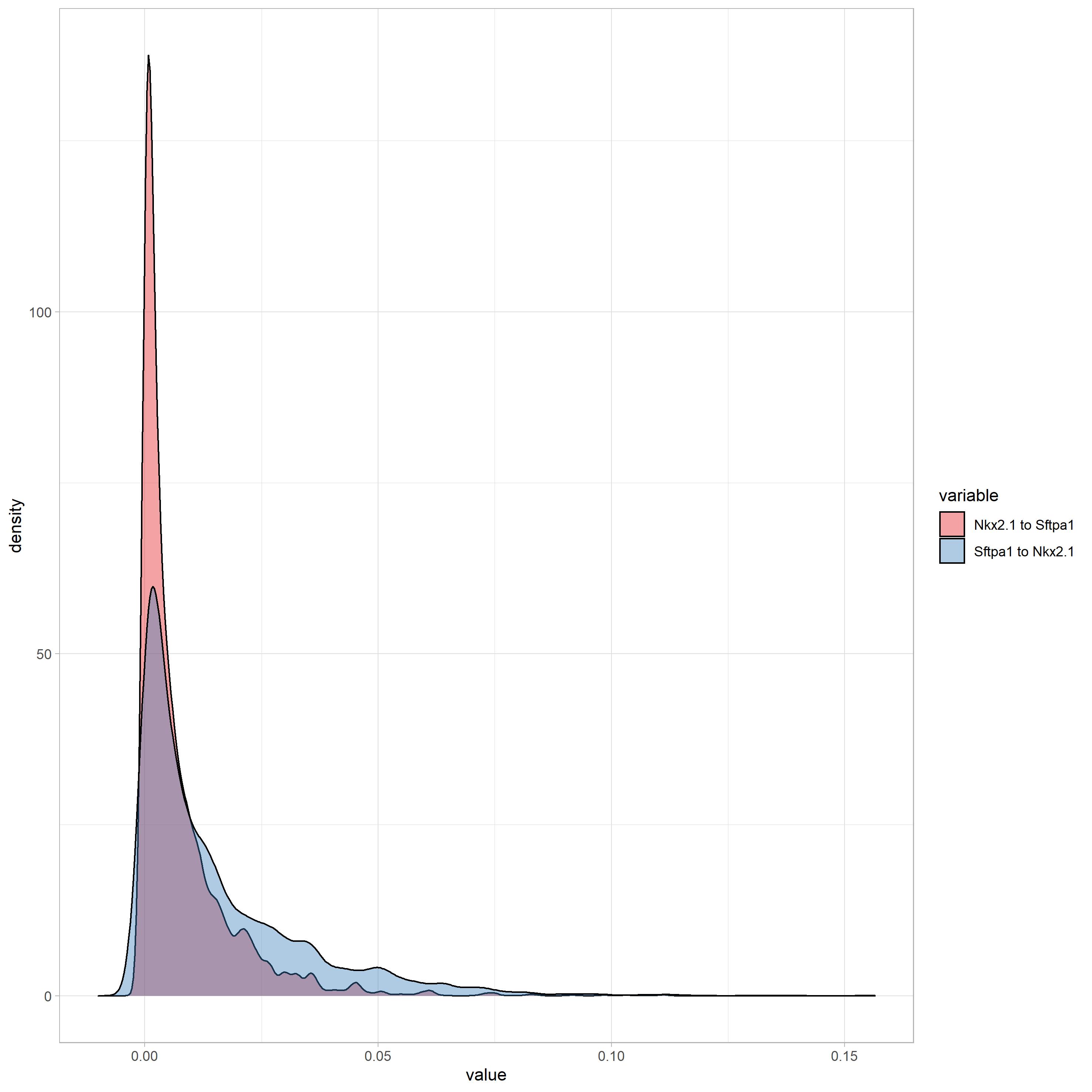
(a) Nkx2.1 and Sftpa1

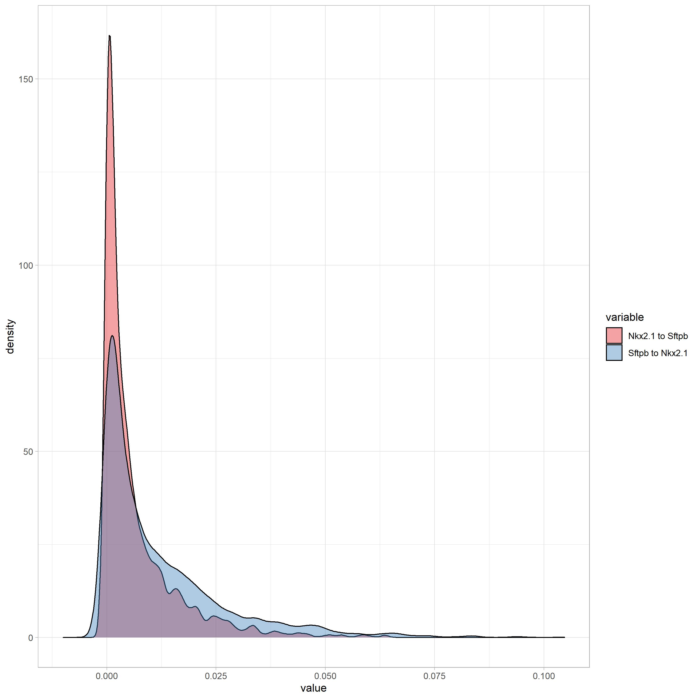
(b) Nkx2.1 and Sftpb

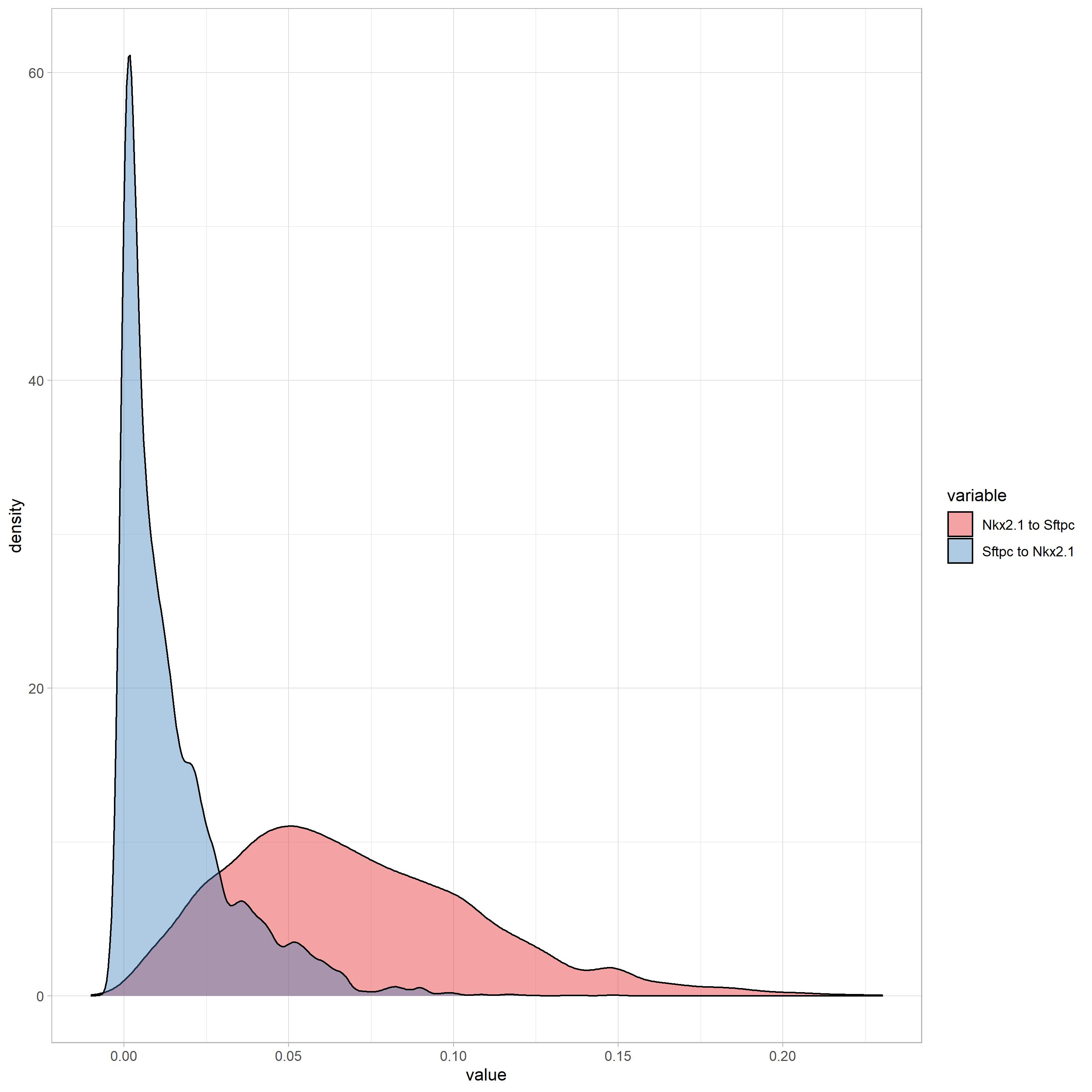
(a) Nkx2.1 and Sftpc

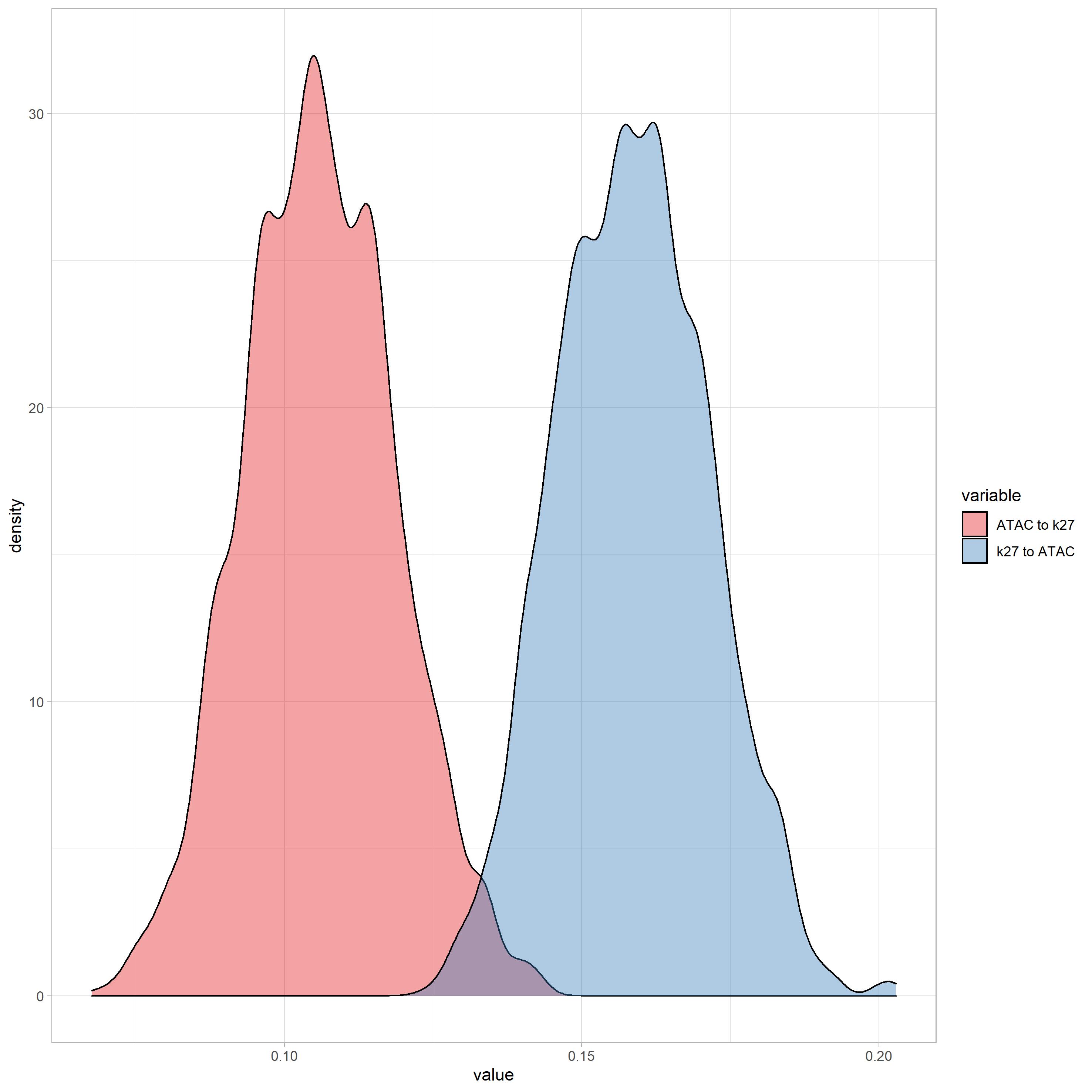
(b) ATAC and k27

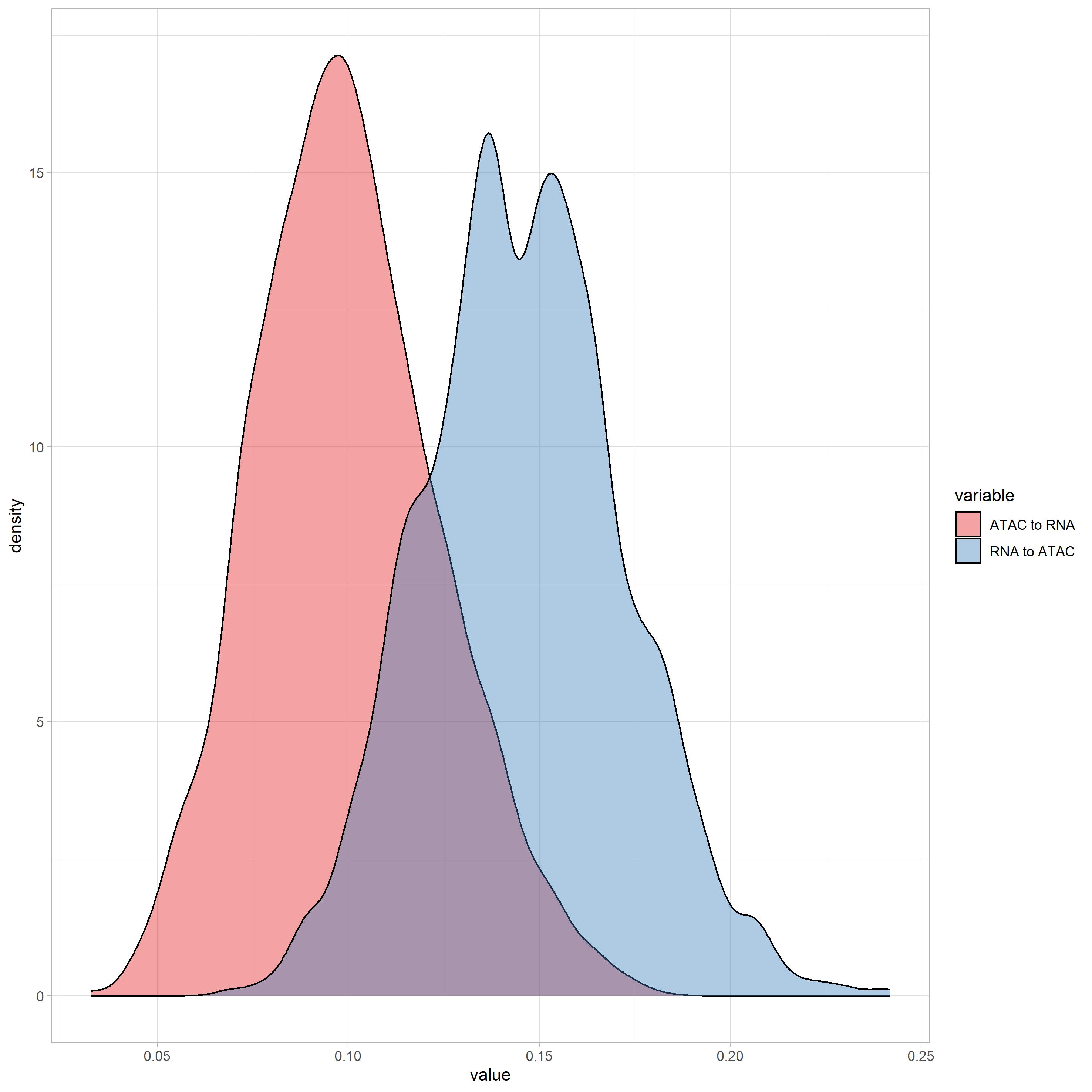
(c) ATAC and RNA

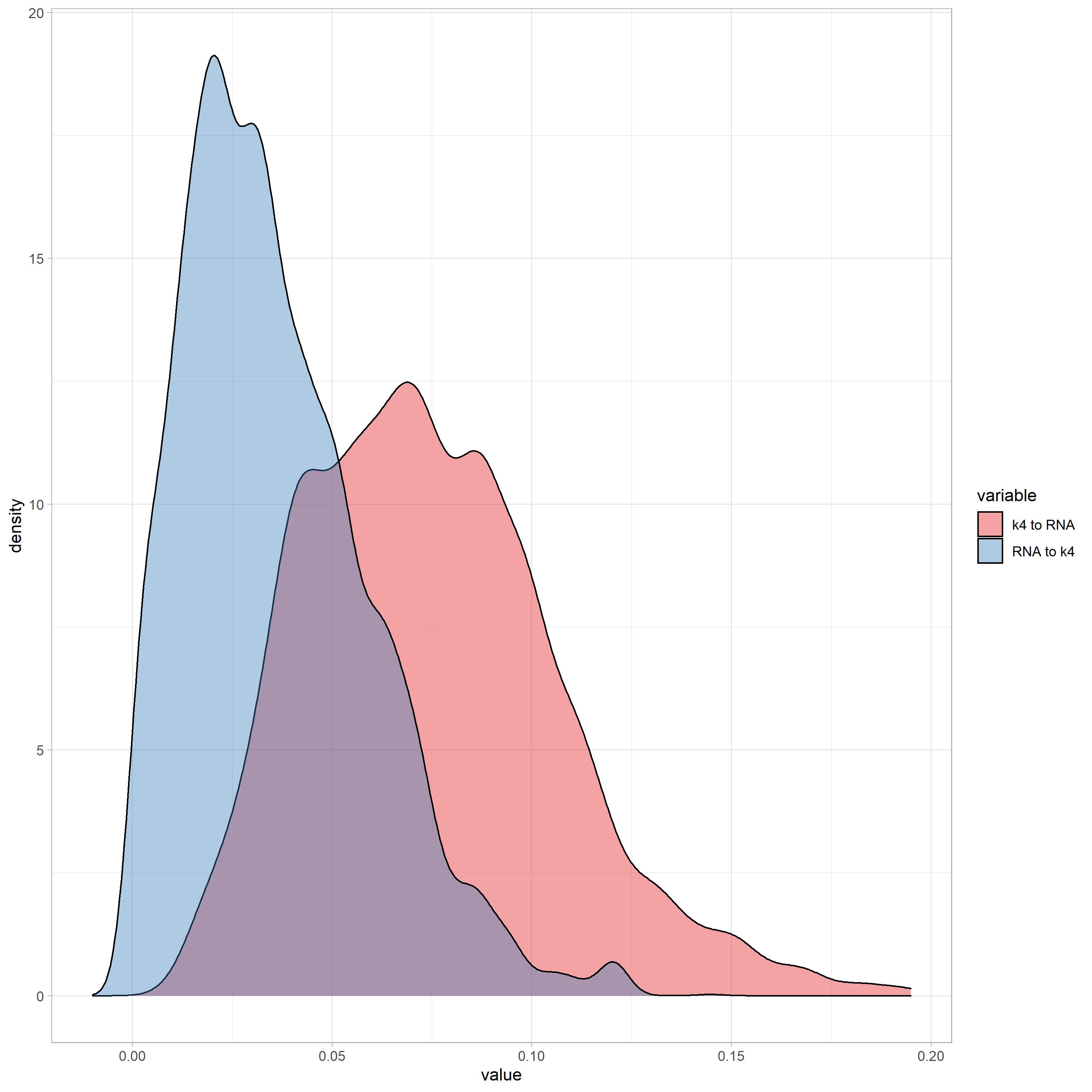
(d) k4 and RNA

Figure 2: Posterior densities of the Bayesian parametric CDD method for each pair of genes. The red densities represent the $\rho_{U\rightarrow V}^{2}$ and the blue the $\rho_{V\rightarrow U}^{2}$ posterior CDD samples.

The parametric Bayesian CDD method was able to capture four out of six correct directionalities. The correct causal relationships that were retrieved are Nkx2.1 $\rightarrow$ Sftpc, H3K27ac $\rightarrow$ ATAC-seq, RNA-seq $\rightarrow$ ATAC-seq and H3K4me3 $\rightarrow$ RNA-seq. Table LABEL:table:3 summarizes the mean values of the estimates of the posterior densities, $\rho_{U\rightarrow V}^{2}$, $\rho_{V\rightarrow U}^{2}$, their difference $\Delta\rho_{U,V}^{2}$ and their ($5\%,95\%$) credible intervals, while Table LABEL:table:4 depicts the probabilities suggesting each direction of influence as a percentage. Figure 2 illustrates the plots for the posterior density distributions for the Bayesian CDD estimates. As presented in Figures 1(a) and 1(b), the posterior directional dependence densities for the pairs Nkx2.1-Sftpa1 and Nkx2.1-Sftpb are highly overlapped, hence the direction of influence is decided only by a few samples. On the other hand, as seen in Figure 2(a), the densities for the pair Nkx2.1-Sftpc are more distinct, with $79\%$ of the posterior samples coming from the correct direction. Overall, the algorithm performed with higher accuracy in the bulk epigenome dataset compared to the scRNA-seq data, as it was able to identify all three directional dependences correctly with a probability of more than $87\%$ in each pair. Furthermore, for genes belonging to the bulk sequencing, the percentage of the frequencies indicating the correct and stronger direction are very high, resulting in distinct and clear posterior distributions as shown in Figures 2(b) to 2(d).

Table 3: Percentage of posterior samples suggesting the direction of influence for each pair of genes for the parametric Bayesian CDD algorithm.

Gene U	Gene V	Samples $\rho^{2}_{U\rightarrow V}>\rho^{2}_{V\rightarrow U}$	Samples $\rho^{2}_{U\rightarrow V}<\rho^{2}_{V\rightarrow U}$
Nkx2.1	Sftpa1	$41.2\%$	$58.8\%$
Nkx2.1	Sftpb	$45.6\%$	$54.4\%$
Nkx2.1	Sftpc	$79\%$	$21\%$
ATAC-seq	H3K27ac	$0.1\%$	$99.9\%$
ATAC-seq	RNA-seq	$8.1\%$	$91.9\%$
H3K4me3	RNA-seq	$87.5\%$	$12.5\%$

The biological interpretation of the inferred directional dependendces are as follows. The gene Nkx2.1 is the transcription factor which regulates proteins Sftpa1, Sftpb and Sftpc. The association between Nkx2.1 and Sftpc was described correctly by both the frequentist and the Bayesian CDD. This result can be explained by the fact that during our exploratory analysis, we noticed that the Sftpc gene was the most highly expressed among the three surfactant proteins, so the results were significant only for this pair. This result is also highlighted visually in the posterior CDD distributions in the Bayesian method in Figure 2(a). The interaction H3K27ac $\rightarrow$ ATAC-seq, implies that the histone mark k27 is enriched at regions that bind proteins. These proteins are the ones that open up chromatin ATAC-seq, the gene that regulates chromatin accessibility. The influence of RNA-seq $\rightarrow$ ATAC-seq was highlighted only by the proposed Bayesian CDD method. The result suggests that variation in RNA-seq is buffered compared to ATAC-seq. A cause for this behaviour, is that RNA-seq is the functional component that gets translated into proteins, hence there exist a mechanism in place to ensure it is not too sensitive to changes in chromatin. Finally, the direction of influence H3K4me3 $\rightarrow$ RNA-seq agrees with the biological interaction as mark enrichment H3K4me3 is always present where gene expression exists, measured from RNA-seq. A comparison of the performance of the two methods is showcased in Table LABEL:table:5.

Table 4: Comparison of performance between the frequentist CDD and the Bayesian CDD methods.The symbol O indicates that the interaction is captured, whereas the symbol X indicates that the gene interaction was not captured by the respective method.

True gene interaction	Frequentist CDD	Bayesian CDD
Nkx2.1 $\rightarrow$ Sftpa1	O	X
Nkx2.1 $\rightarrow$ Sftpb	X	X
Nkx2.1 $\rightarrow$ Sftpc	O	O
H3K27ac $\rightarrow$ ATAC-seq	O	O
RNA-seq $\rightarrow$ ATAC-seq	X	O
H3K4me3 $\rightarrow$ RNA-seq	O	O

5 Conclusion

In this work, causal inference among gene pairs of both single-cell and bulk sequencing data was investigated. Copula based methods were chosen to be practised, since they are able to isolate the marginal effect of the distributions from the joint behaviour. That way, one is able to consider the direction of influence through a functional of the copula structure, where the direction of the dependence lies. Frequentist Copula Directional Dependence introduced by Kim and Hwang (2017) and our novel proposed method of Bayesian Copula Directional Dependence, were applied on two gene expression data sets. Their performance was evaluated in terms of their ability to produce accurate and informative results according to the true biological interaction between the genes.

A common observation for both methods is that no particular copula function was applied to the data, since there was no prior evidence that a specific family is appropriate. This is extremely useful for implementations where only the directionality rather than the complete dependence structure is of interest. The CDD measures infer connectivity, so the relative strengths of the directional dependences can be compared between gene pairs, based on nonlinear copula regression models. Although the frequentist CDD retrieved four out of six interactions, the results were not promising, as the directional dependence estimates and their confidence intervals were highly underestimated. On the other hand, the parametric Bayesian CDD approach outperformed the frequentist method, by producing more robust credible intervals and clear distinguishable posteriors distributions. It is noted that for both the frequentist and parametric Bayesian CDDs, the conditional marginals were assumed to follow a Beta distribution and the original marginals were uniformly distributed. This implies that the overall improvement was due to the uncertainty applied to the estimates of the functional of the dependence structure and not on the marginal estimation. To conclude, our newly proposed parametric Bayesian CDD algorithm, can be used for the exploration and construction of gene interactions providing an insight into the architecture and functionality of genetic systems.

6 Acknowledgements

This work was supported by the ARC Centre of Excellence for Mathematical and Statistical Frontiers (Project ID: CE140100049). We would like to thank Dr Emily Wong from the Victor Chang Cardiac Research Institute for providing us with the data and for her help with the biological interpretation of the results.

References

- Bernstein et al. [2007] Bradley E. Bernstein, Alexander Meissner, and Eric S. Lander. The mammalian epigenome. Cell, 128(4):669––681, 2007.
- Bornholdt [2008] Stefan Bornholdt. Boolean network models of cellular regulation: prospects and limitations. Journal of the Royal Society Interface, 5(suppl_1):S85–S94, 2008.
- Buenrostro et al. [2013] Jason D Buenrostro, Paul G Giresi, Lisa C Zaba, Howard Y Chang, and William J Greenleaf. Transposition of native chromatin for multimodal regulatory analysis and personal epigenomics. Nature methods, 10(12):1213, 2013.
- Cao et al. [2010] Yuxia Cao, Tiffany Vo, Guetchyn Millien, Jean-Bosco Tagne, Darrell Kotton, Robert J Mason, Mary C Williams, and Maria I Ramirez. Epigenetic mechanisms modulate thyroid transcription factor 1-mediated transcription of the surfactant protein b gene. Journal of Biological Chemistry, 285(3):2152–2164, 2010.
- Chen et al. [2005] Kuang-Chi Chen, Tse-Yi Wang, Huei-Hun Tseng, Chi-Ying F Huang, and Cheng-Yan Kao. A stochastic differential equation model for quantifying transcriptional regulatory network in saccharomyces cerevisiae. Bioinformatics, 21(12):2883–2890, 2005.
- Clayton [1978] David G Clayton. A model for association in bivariate life tables and its application in epidemiological studies of familial tendency in chronic disease incidence. Biometrika, 65(1):141–151, 1978.
- Deng et al. [2005] Xutao Deng, Huimin Geng, and Hesham Ali. Examine: A computational approach to reconstructing gene regulatory networks. BioSystems, 81(2):125–136, 2005.
- Dodge and Rousson [2000] Yadolah Dodge and Valentin Rousson. Direction dependence in a regression line. Communications in Statistics-Theory and Methods, 29(9-10):1957–1972, 2000.
- Dubitzky et al. [2013] Werner Dubitzky, Olaf Wolkenhauer, Hiroki Yokota, and Kwang-Hyun Cho. Encyclopedia of systems biology. Springer Publishing Company, Incorporated, 2013.
- Ferrari and Cribari-Neto [2004] Silvia Ferrari and Francisco Cribari-Neto. Beta regression for modelling rates and proportions. Journal of applied statistics, 31(7):799–815, 2004.
- Friedman et al. [2000] Nir Friedman, Michal Linial, Iftach Nachman, and Dana Pe’er. Using bayesian networks to analyze expression data. Journal of computational biology, 7(3-4):601–620, 2000.
- Grazian and Liseo [2017] Clara Grazian and Brunero Liseo. Approximate bayesian inference in semiparametric copula models. Bayesian Analysis, 12(4):991–1016, 2017.
- Guolo and Varin [2014] Annamaria Guolo and Cristiano Varin. Beta regression for time series analysis of bounded data, with application to canada google® flu trends. Annals of Applied Statistics, 8(1):74–88, 2014.
- Huynh et al. [2014] Van-Nam Huynh, Vladik Kreinovich, and Songsak Sriboonchitta. Modeling dependence in econometrics. Springer, 2014.
- Kim and Kim [2014] Daeyoung Kim and Jong-Min Kim. Analysis of directional dependence using asymmetric copula-based regression models. Journal of Statistical Computation and Simulation, 84(9):1990–2010, 2014.
- Kim et al. [2014] J Kim, Y Jung, and EA Sungur. Copulas with directional dependence property: Application to foreign exchange currency data. Models Assisted Statistics and Applications, 9:309–324, 2014.
- Kim and Hwang [2017] Jong-Min Kim and Sun-Young Hwang. Directional dependence via gaussian copula beta regression model with asymmetric garch marginals. Communications in Statistics-Simulation and Computation, 46(10):7639–7653, 2017.
- Kim et al. [2008] Jong-Min Kim, Yoon-Sung Jung, Engin A Sungur, Kap-Hoon Han, Changyi Park, and Insuk Sohn. A copula method for modeling directional dependence of genes. BMC bioinformatics, 9(1):1–12, 2008.
- Kim et al. [2009] Jong-Min Kim, Yoon-Sung Jung, and Tim Soderberg. Directional dependence of genes using survival truncated fgm type modification copulas. Communications in Statistics-Simulation and Computation, 38(7):1470–1484, 2009.
- Lambert and Vandenhende [2002] Philippe Lambert and Francois Vandenhende. A copula-based model for multivariate non-normal longitudinal data: analysis of a dose titration safety study on a new antidepressant. Statistics in medicine, 21(21):3197–3217, 2002.
- Masarotto and Varin [2012] Guido Masarotto and Cristiano Varin. Gaussian copula marginal regression. Electronic Journal of Statistics, 6:1517–1549, 2012.
- Muddapur [2003] MV Muddapur. On directional dependence in a regression line. Communications in Statistics-Theory and Methods, 32(10):2053–2057, 2003.
- Nikoloulopoulos and Karlis [2008] Aristidis K Nikoloulopoulos and Dimitris Karlis. Multivariate logit copula model with an application to dental data. Statistics in Medicine, 27(30):6393–6406, 2008.
- Santos-Rosa et al. [2002] Helena Santos-Rosa, Robert Schneider, Andrew J Bannister, Julia Sherriff, Bradley E Bernstein, NC Tolga Emre, Stuart L Schreiber, Jane Mellor, and Tony Kouzarides. Active genes are tri-methylated at k4 of histone h3. Nature, 419(6905):407–411, 2002.
- Shmulevich et al. [2002] Ilya Shmulevich, Edward R Dougherty, Seungchan Kim, and Wei Zhang. Probabilistic boolean networks: a rule-based uncertainty model for gene regulatory networks. Bioinformatics, 18(2):261–274, 2002.
- Sims III et al. [2003] Robert J Sims III, Kenichi Nishioka, and Danny Reinberg. Histone lysine methylation: a signature for chromatin function. TRENDS in Genetics, 19(11):629–639, 2003.
- Sklar [1959] M Sklar. Fonctions de repartition an dimensions et leurs marges. Publications de l’Institut de Statistique de L’Universit de Paris, 8:229–231, 1959.
- Sungur [2005a] Engin A Sungur. A note on directional dependence in regression setting. Communications in Statistics—Theory and Methods, 34(9-10):1957–1965, 2005a.
- Sungur [2005b] Engin A Sungur. Some observations on copula regression functions. Communications in Statistics—Theory and Methods, 34(9-10):1967–1978, 2005b.
- Thomas [1973] René Thomas. Boolean formalization of genetic control circuits. Journal of theoretical biology, 42(3):563–585, 1973.
- Vijesh et al. [2013] Nedumparambathmarath Vijesh, Swarup Kumar Chakrabarti, and Janardanan Sreekumar. Modeling of gene regulatory networks: A review. Journal of Biomedical Science and Engineering, 6(02):223, 2013.
- Zou and Conzen [2005] Min Zou and Suzanne D Conzen. A new dynamic bayesian network (dbn) approach for identifying gene regulatory networks from time course microarray data. Bioinformatics, 21(1):71–79, 2005.