LlamaTune: Sample-Efficient DBMS Configuration Tuning

Abstract.

Tuning a database system to achieve optimal performance on a given workload is a long-standing problem in the database community. A number of recent works have leveraged ML-based approaches to guide the sampling of large parameter spaces (hundreds of tuning knobs) in search for high performance configurations. Looking at Microsoft production services operating millions of databases, sample efficiency emerged as a crucial requirement to use tuners on diverse workloads.

This motivates our investigation in LlamaTune, a tuner design that leverages domain knowledge to improve the sample efficiency of existing optimizers. LlamaTune employs an automated dimensionality reduction technique based on randomized projections, a biased-sampling approach to handle special values for certain knobs, and knob values bucketization, to reduce the size of the search space. LlamaTune compares favorably with the state-of-the-art optimizers across a diverse set of workloads. It identifies the best performing configurations with up to $11\times$ fewer workload runs, and reaching up to $21\%$ higher throughput. We also show that benefits from LlamaTune generalize across both BO-based and RL-based optimizers, as well as different DBMS versions.

While the journey to perform database tuning at cloud-scale remains long, LlamaTune goes a long way in making automatic DBMS tuning practical at scale.

PVLDB Reference Format:
PVLDB, 15(11): 2953 - 2965, 2022.
doi:10.14778/3551793.3551844

PVLDB Artifact Availability:
The source code, data, and/or other artifacts have been made available at %leave␣empty␣if␣no␣availability␣url␣should␣be␣sethttps://github.com/uw-mad-dash/llamatune.

1. Introduction

Tuning the configuration of a database management system (DBMS) is necessary to achieve high performance. While DBMS tuning has been traditionally performed manually, e.g., by DB administrators, the shift to cloud computing, the increasing diversity of workloads and the large number of configuration knobs (Storm et al., 2006; Duan et al., 2009) makes it challenging to manually tune databases for high performance. As a result, a number of automated methods (Van Aken et al., 2017; Duan et al., 2009; Cereda et al., 2021; Zhang et al., 2021b, 2019; Li et al., 2019; Gur et al., 2021; Zhu et al., 2017; Wang et al., 2021) for tuning have been proposed, with recent methods using machine learning (ML). ML-based methods have been shown to generalize to a number of workloads (Zhang et al., 2021a) and can find configurations that achieve up to 3-6$\times$ higher throughput (or lower latency) (Li et al., 2019; Van Aken et al., 2017; Zhang et al., 2019) when compared to using manually-tuned configurations.

There are two main classes of ML-based approaches: those that perform prior training on selected benchmarks and transfer (or fine-tune) this knowledge given new customer workloads (e.g., OtterTune (Van Aken et al., 2017) and CDBTune (Zhang et al., 2019)), and those (Li et al., 2019; Duan et al., 2009; Cereda et al., 2021) that directly tune a new customer workload by iteratively selecting a configuration using an optimizer, and running workloads with them (Figure 1). Algorithms used in these configuration optimizers try to balance between exploring unseen regions of the configuration search space, and exploiting the knowledge gathered until that point. Search-based methods (Zhu et al., 2017), RL-based methods (Li et al., 2019) or Bayesian Optimization (BO) methods (Cereda et al., 2021; Duan et al., 2009) are commonly used, though a recent study (Zhang et al., 2021a) found that SMAC (Hutter et al., 2011), a BO-based method, performed best for DBMS tuning.

In both settings, the cost and time involved in exploring several configurations before reaching a chosen one is the core challenge for practical relevance. Based on our visibility into production services operating millions of databases in Azure, we find that sample efficiency (i.e., how few workload runs does it take to reach a given level of performance) is crucial to scale autotuning across diverse workloads. Currently, state-of-the-art methods require 100 or more iterations (Zhang et al., 2021a) to converge to a good configuration, with each iteration taking several minutes. To this purpose we focus our investigation in developing techniques that can improve sample efficiency, and that are broadly complementary to existing work.

We observe that existing optimizers do not leverage expert knowledge about the system they are tuning and using domain knowledge has the potential to significantly improve sample efficiency. First, based on our prior work (Kanellis et al., 2020) (and others (Van Aken et al., 2021; Zhang et al., 2021a)) we find that tuning a few important knobs is sufficient for achieving high DBMS performance, and tuning a smaller configuration space can lead to significant improvements in the number of samples required (Zhang et al., 2021a). Yet, which knobs are important varies by workload, and existing methods for identifying important knobs are expensive and can be unreliable (Section 2.3). Second, we observe that not all DBMS knob values are the same. For example, in PostgreSQL, the flag backend_flush_after denotes the number of pages after which previously performed writes are flushed to disk. However, the flag has a special meaning when set to 0, disabling forced writeback and letting the OS manage it. Such special values can affect the system in unpredictable ways and existing optimizers are unaware of such behaviors. Additionally, we note that some parameters may have very large valid ranges. For instance, shared_buffers is given as the number of 8K pages to account for potentially 100s of GBs. Yet, the effect on performance between two nearby values, (e.g., 100 vs. 101), may be negligible. These insights lead us to ask: How can we build a domain knowledge-aware configuration tuner that can minimize the number of samples required without sacrificing the final DBMS performance achieved?

Contributions We address these challenges in LlamaTune with the following contributions. First, we show that surprisingly it is possible to achieve the benefits of only tuning important knobs but without using any prior knowledge. Specifically, we leverage a randomized low-dimensional projection approach (Nayebi et al., 2019) where we perform a projection of the configuration space from all dimensions ($D$) to a lower-dimensional subspace ($d$) and then use the optimizer to tune this smaller subspace. We also discuss how such a method can be integrated with a DBMS and handle categorical and numerical knobs. Second, to handle knobs that have a different behavior for special values, we design a new biased-sampling based approach. This makes the optimizer aware of the special case behavior with high probability during its random initialization phase and minimizes the number of samples required to find good configurations. To address large value ranges, we experiment with bucketizing nearby values into groups (e.g., 100MB increments) to further reduce the search space that needs to be explored. We find that this can improve convergence without sacrificing much from the performance of the optimal configuration for some workloads.

We combine the above techniques to design LlamaTune , an end-to-end tuning framework that can tune a DBMS for new workloads without using any prior knowledge. We integrate LlamaTune with three state-of-the-art optimizers: two BO-based ones (SMAC (Hutter et al., 2011), GP-BO (Ru et al., 2020)), and an RL-based one (DDPG (Zhang et al., 2019)). We evaluate LlamaTune using six popular OLTP workloads and consider scenarios where we tune for optimizing throughput or tail latency (95th percentile). Our results show that LlamaTune can converge to the optimal configuration up to $11\times$ faster than SMAC while also reaching up to $20.85\%$ higher throughput. We also demonstrate that similar gains can be achieved when LlamaTune is used with GP-BO, or DDPG. Finally, we also detail the process and our experiences of porting LlamaTune to a newer DBMS version, and show that LlamaTune can deliver meaningful gains with little effort.

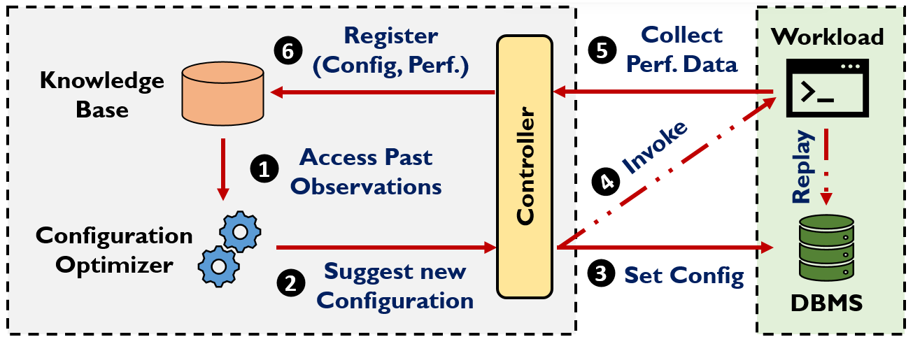
Figure 1. Overview of DBMS Knob Tuning Procedure

2. Preliminaries

In this section, we formalize the DBMS knob configuration problem and discuss existing methods for tuning. Then, we identify some limitations of existing tuners and opportunities for improvements.

2.1. Background and Related Work

2.1.1. Automatic Database Tuning

We can formulate database knob configuration tuning as an optimization problem. Consider as input, a set of set of $n$ knobs, $\theta_{1},\ldots,\theta_{n}$, alongside their respective domains $\Theta_{1},\ldots,\Theta_{n}$. These knobs domains can be either continuous, discrete, or categorical. Given this set of knobs, the resulting configuration space can be defined as $\Theta=\Theta_{1}\times\ldots\times\Theta_{n}$. We assume a performance metric is encoded by the objective function $f:\Theta\to\mathbb{R}$, that assigns a single performance value to each configuration. Common performance metrics used in database tuning include system throughput, or tail latency (e.g., $95$th percentile latency). Retrieving the value $f$ at some configuration point $\theta$ requires measuring this performance metric when the system is executed with $\theta$. Given a workload, the goal of database tuning is to find a configuration $\theta^{*}$ that maximizes (or minimizes) the target metric: $\theta^{*}=\operatorname*{argmax}_{\theta\in\Theta}f(\theta)$

Most database knob tuning frameworks are built around a common architecture and the main components include (i) a knowledge base (KB), (ii) a configuration optimizer, and (iii) an experiment controller. The knowledge base holds a record of all previously evaluated samples, $\mathcal{D}=\{\theta^{j},f(\theta^{j})\}$, and gets updated every time a new configuration is evaluated. The configuration optimizer leverages the knowledge base to recommend configuration points $\theta^{j}$ that are promising (i.e., may lead to higher performance). Finally, given a configuration, the controller orchestrates the execution of the workload and propagating the results (i.e., $\theta^{j},f(\theta^{j})$) back to KB.

Assuming a fixed workload, the tuning process is iterative as shown in Figure 1. At first, the optimizer uses the current knowledge base, in order to suggest a configuration that it expects to improve performance. Then, this configuration is applied to the DBMS instance running on a separate testing environment (green-shaded area). Subsequently, the controller invokes the workload that feeds queries to the DBMS; the workload usually runs for several (e.g., $5$-$10$) minutes. Once the workload execution completes, the controller collects the performance data (e.g., throughput) and any related metrics (e.g., internal DBMS metrics), and forwards them to the knowledge base, which is then updated with the observation (i.e., configuration, measured performance pair). The above process is repeated until a certain budget $T$ (e.g., number of iterations, time, or cost limit) is exhausted.

Based on how much prior knowledge is available at the start of the tuning process, one can categorize various auto-tuners proposed in prior literature. Some tuning frameworks (Van Aken et al., 2017; Zhang et al., 2019; Li et al., 2019; Duan et al., 2009) assume that before the tuning process begins, the KB has already been populated with prior observations. In particular, these frameworks rely upon an initial profiling (or training) phase that includes evaluating thousands configuration points using benchmark workloads (e.g., up to $30$K for OtterTune (Van Aken et al., 2017)). This way, they can leverage prior knowledge gained from the training phase in order to propose good-performing configurations for new workloads. Other tuning frameworks (Zhu et al., 2017; Cereda et al., 2021; Wang et al., 2021) begin the tuning process without any prior knowledge: i.e., the KB is initially empty. Starting from zero knowledge, these tuners can only use the aforementioned tuning process to gather knowledge about the workload or the DBMS. To combat this challenge, these tuners typically use algorithms that try to balance between exploring unseen regions of the configuration search space, and exploiting the knowledge gathered so far. As the tuning process progresses and the KB accumulates more samples, these frameworks are eventually able to find configurations that achieve good performance.

In the above architecture, we can see that the configuration optimizer used plays a key role in determining the time (and hence cost) it takes to find a good performing configuration. Thus, we next survey configuration optimizers used in prior work.

2.2. Configuration Optimizers

The configuration optimizer methods used by prior works can be classified into three categories: (i) Search-based, (ii) Reinforcement Learning (RL) based, and (iii) Bayesian Optimization (BO) based.

A popular example of a search-based method is BestConfig (Zhu et al., 2017), which employs heuristics to divide the search space into multiple segments and navigates it through branch and bound policies. Even though it can quickly choose which points to evaluate next, it does not makes use of a KB, which has been shown to hurt its performance (Cereda et al., 2021). Reinforcement learning methods proposed in (Zhang et al., 2019; Li et al., 2019; Gur et al., 2021) leverage the Deep Deterministic Policy Gradient (DDPG) algorithm (Lillicrap et al., 2019), which trains an RL actor using a trial-and-error approach. The actor utilizes a deep neural network that is trained based on DBMS internal metrics, and can propose configurations that balance exploration and exploitation. In general, for RL methods to work well, thousands of samples have to be evaluated (Li et al., 2019) and prior work (Zhang et al., 2021a) has found that RL based methods require more iterations due to the complexity of the neural networks used.

The majority of prior database auto-tuners use BO-based methods (Van Aken et al., 2017; Duan et al., 2009; Cereda et al., 2021; Zhang et al., 2021b; Dalibard et al., 2017). Bayesian optimization is a gradient-free, sequential, model-based approach that aims to find the optimum of an expensive-to-evaluate unknown function $f$, by evaluating as few samples as possible (Shahriari et al., 2015). It also handles cases where the evaluated samples $f(\theta^{j})$ are noisy. BO consists of two main components: the surrogate model, and the acquisition function. A surrogate model is an ML model, which given a set of observations $f(\theta^{k})$, constructs an approximation of $f$; this approximation is refined each time a new point is evaluated. The acquisition function is used to choose which point to evaluate next. To do so, it uses the surrogate model to compute the expected utility of many candidate points, and then selects the one with the highest utility. Utility values are calculated such that BO can effectively trade-off between the exploration of unseen regions, and the exploitation of good-performing ones.

While there are many BO variants, database knob tuners (Van Aken et al., 2017; Duan et al., 2009; Zhang et al., 2021b) have typically used “vanilla” Gaussian process (GP) as their surrogate model. However, a recent comprehensive evaluation (Zhang et al., 2021a) of different BO variants shows that GP is not the optimal choice for database knob configuration tuning. After experimenting with many modern black-box optimizers (including the ones used for database tuning (Van Aken et al., 2017; Duan et al., 2009; Cereda et al., 2021; Zhang et al., 2021b)) this study (Zhang et al., 2021a) concluded that the best performing optimizer was SMAC (i.e., Sequential Model-based Algorithm Configuration) (Hutter et al., 2011). SMAC uses a random forest (RF) surrogate model, and is shown to perform very well in high-dimensional and heterogeneous search spaces, consisting of continuous, discrete, and categorical knobs. Compared to vanilla GPs, RFs can inherently support categorical features, which helps find better configurations while also converging faster (Hutter et al., 2011). Another method that improves over vanilla GP uses two separate kernels, Matérn and Hamming, for continuous and categorical features, respectively. This GP variant, which we refer to as GP-BO (Ru et al., 2020), also showed promising performance when dealing with a mixed search space, and a moderate number (i.e., up to $20$) of dimensions (Zhang et al., 2021a).

In this work we focus on designing a domain knowledge-aware configuration optimizer and show that our techniques can be integrated with SMAC, GP-BO, and DDPG..

2.3. Motivation

2.3.1. Only Tuning Important Knobs

While database tuners that start with zero knowledge are able to suggest good-performing configurations eventually, they typically require many iterations until they can do so. For instance, using the current state-of-the-art BO-variant, SMAC (Hutter et al., 2011), still requires around $100$ samples to reach optimal performance for most workloads (Zhang et al., 2021a). With each sample evaluation (or iteration) taking $5-10$ minutes, the overall tuning process takes 8-16 hours. The main reason optimizers need a large number of iterations is that the configuration search space exposed to them is very high-dimensional. The size of these search spaces are typically proportional to the number of configuration knobs that the user wishes to tune and this can include hundreds of knobs for popular databases like Postgres or MySQL (Van Aken et al., 2017).

Table 1. SHAP’s top-8 knobs vs hand-picked ones for YCSB-A. Underlined knobs indicate the differences between the two.

SHAP (top-8)	Hand-picked (top-8)
autovacuum_vacuum_threshold	autovacuum_analyze_scale_factor
autovacuum_vacuum_scale_factor	autovacuum_vacuum_scale_factor
commit_delay	commit_delay
enable_seqscan	full_page_writes
full_page_writes	geqo_selection_bias
geqo_selection_bias	max_wal_size
shared_buffers	shared_buffers
wal_writer_flush_after	wal_writer_flush_after

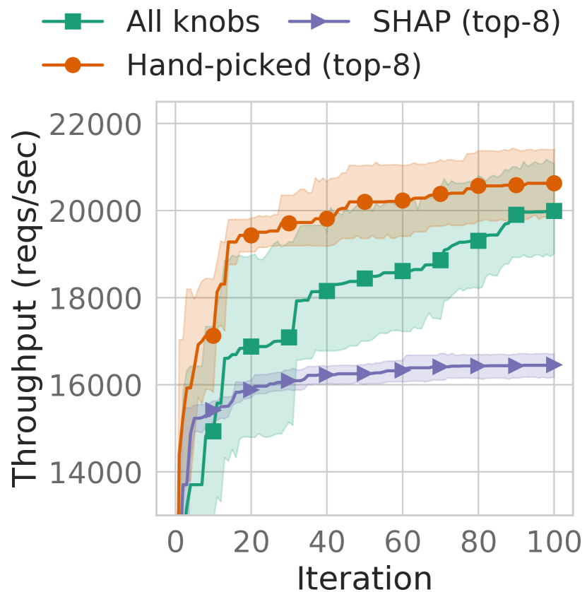
(a) SHAP vs Manual (YCSB-A)

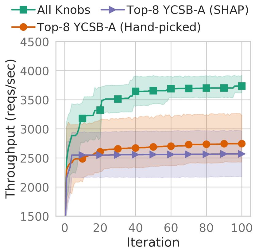
(b) Top-8 YCSB-A to TPC-C

Figure 2. Best performance on YCSB-A, when tuning SHAP’s top-8 knobs; hand-picked top-8 knobs, and all knobs are baselines (left plot). Best performance on TPC-C, when tuning YCSB-A’s top-8 knobs (SHAP, hand-picked) (right plot).

However, recent studies have shown that tuning a handful of knobs can be sufficient to achieve near-optimal performance and significantly reducing the number of knobs can accelerate the tuning process (Kanellis et al., 2020; Van Aken et al., 2021; Zhang et al., 2021a). Intuitively, the configuration search space generated by few (important) knobs is much smaller than the one when considering all knobs, making BO-based methods much more effective at finding configurations that yield good performance (Shahriari et al., 2015; Van Aken et al., 2021). However, it still remains challenging to identify and select the correct set of important knobs for different workloads or systems.

2.3.2. Identifying Important Knobs

All existing methods for automatically identifying important knobs use a ranking-based process (Kanellis et al., 2020; Van Aken et al., 2021; Zhang et al., 2021a). Ranking-based methods typically use a space-filling sampling, like Latin Hypercube Sampling (LHS) (McKay et al., 1979), to generate and evaluate thousands of configurations. With this set of evaluated configurations alongside the measured performance, an ML model is trained to quantify how each knob affects the DBMS performance, an i.e., importance score. Recent work (Zhang et al., 2021a) has shown that SHAP (Lundberg and Lee, 2017) values provide the most meaningful importance score in the context of DBMS tuning. SHAP uses a game-theoretic approach to break down the impact of each individual feature when analyzing the performance deviation from the default configuration.

Although these statistical methods do not require any human input for computing the important knob ranking, they require evaluating thousands of data samples (Kanellis et al., 2020; Van Aken et al., 2021). Thus, using important knob ranking to prune the configuration space is not useful in a setting where we start with zero knowledge. Moreover, as we discuss next, methods that identify important knobs are (1) not always reliable, which can lead to finding worse configurations, and (2) the important knobs found for one workload may not work for others.

Limitations of ranking important knobs. Using the read-write balanced YCSB-A (Cooper et al., 2010) as our workload, we generate (using LHS) and evaluate $2,500$ configurations for PostgreSQL v9.6, where we vary the values of $90$ knobs. Following prior work (Zhang et al., 2021a), we employ SHAP (using RF) to rank all knobs in descending order of importance. From this ranking, we select the top eight ones, which, according to SHAP, should be able to provide most of the tuning performance gains. We also consider two baselines: the full set of $90$ knobs, and a hand-picked set of eight important knobs, which differs slightly from the SHAP-based one. Table 1 shows both important knob sets.

Given these three sets, we launch a tuning session using SMAC for $100$ iterations, optimizing for throughput; we repeat the experiment five times with different random seeds. 2(a) shows the best throughput reached at each iteration; shaded regions correspond to [5%, 95%] confidence intervals. We make two observations. First, tuning SHAP’s top-8 knobs achieves worse final throughput compared to both the hand-picked top-8 knobs, and all knobs. Thus, while it is possible to reduce the number of knobs tuned and still achieve optimal performance (e.g., hand-picked top-8 knobs), SHAP’s ranking fails to extract the “correct” set of important knobs. Second, tuning the hand-picked top-8 set of knobs identifies a better-performing configuration, while also converging much faster. Therefore, exploring the appropriate low-dimensional configuration space, can greatly benefit the performance of BO methods.

We next study the issue of transferring important knobs across workloads. Using SHAP’s important knobs for YCSB-A, we launch a similar experiment for a different workload, TPC-C (Figure 2(b)). We observe that when tuning all knobs, SMAC reaches a significantly higher throughout compared to only tuning the top-8 knobs from YCSB-A. Thus, reusing a set of important knobs derived from one workload to tune another, does not always lead to gains.

In summary, we see that tuning a low-dimensional space, generated by a set of important knobs can lead to finding better configurations with fewer iterations compared to the state-of-the-art SMAC algorithm. However, existing statistical-based methods for selecting important knobs cannot be utilized as they are expensive, not always reliable and can lead to worse tuning outcomes.

3. Low-Dimensional Tuning

In this section, we present a new approach which bypasses the need to identify the exact set of important knobs, yet realizes the benefits of low-dimensional tuning.

Setup. We consider a scenario where a user/operator is tuning a DBMS for a specific workload given no prior knowledge. Given $D$ tuning knobs, a $D$-dimensional space $X_{D}$ is constructed to represent the configuration search space. Each point $p\in X_{D}$ corresponds to a specific DBMS configuration, where $p$’s coordinates determine the value of each of the $D$ tuning knobs. This space is then given as input to a BO optimizer (e.g., SMAC), whose goal is to model the DBMS performance at each point $p\in X_{D}$. Due to the high dimensionality $D$ of the input search space $X_{D}$, modeling the DBMS performance across the whole space accurately requires the evaluation of many points (configurations). Yet, as we’ve seen, many of those parameters those dimensions represent are less important, and hence amenable to compression in a model. With this in mind, if instead of the input space $X_{D}$, the BO method received as an input, a smaller $d$-dimensional space $X_{d}$, where $d<<D$, then fewer points would be needed to effectively learn the (smaller) space $X_{d}$. Thus, choosing a smaller space $X_{d}$ instead of $X_{D}$ has the potential to improve the optimizer performance: i.e., find better configurations or similar-performing ones, faster.

However, not every reduced space $X_{d}$ may lead to benefits. For example, tuning an $1$-dimensional space generated by a single non-important knob would not lead to any performance improvements. Therefore, it is vital for this smaller space $X_{d}$ to include DBMS configurations that can achieve high performance; ideally the best-performing ones. Given this, we set the following goal:

For a user-provided $D$-dimensional input configuration space $X_{D}$, devise an approximation using some $d$-dimensional space $X_{d}$, where $d<<D$, which is likely to contain at least one point $p^{\prime}\in X_{d}$ that can yield performance close to the optimal $p^{*}\in X_{D}$.

3.1. Synthetic Search Spaces

The low dimensional spaces we discussed in Section 2.3 assumed that each dimension of the space corresponds to a specific configuration knob. While this makes it easier for us to envision this space, it makes no difference for the optimizer, which can be given any search space as input. To this end, we now decouple this one-to-one relationship of configuration knobs to input search space dimensions. In particular, we can use “artificial” dimensions (or synthetic knobs) to generate our low dimensional space, $X_{d}$. These synthetic knobs do not have any physical meaning themselves, yet their values determine the values of one (or more) DBMS configuration knobs. In other words, one can define a mapping from the synthetic knob values (i.e., approximated space $X_{d}$), to the physical DBMS configuration knobs (i.e., original input space $X_{D}$). This enables us to realize the benefits of optimizing a low-dimensional space, while avoiding the need to identify important knobs.

The idea of using a synthetic smaller space $X_{d}$ to implicitly optimize a high-dimensional input search space $X_{D}$, has been recently studied in the BO community (Eriksson and Jankowiak, 2021; Wang et al., 2016). Multiple theoretically-sound approaches have been proposed to define this space, construct the mapping between the two spaces $X_{d}$, $X_{D}$, and/or extend the standard BO algorithm to better navigate through this smaller space (Eriksson and Jankowiak, 2021; Wang et al., 2016; Nayebi et al., 2019; Letham et al., 2020). For these methods to be effective, the target objective function should be affected by a small subset of the original high-dimensional space. If $d_{e}$ is the size of this subset, for a low-dimensional space $X_{d}$ with $d>d_{e}$, these methods provide theoretical guarantees that with high probability, each $p\in X_{D}$ can be obtained by projecting some point $p^{\prime}\in X_{d}$. In other words, if the low-dimensional space is larger than the effective dimensionality of the objective function, then it is possible to achieve near-optimal performance just by tuning this smaller space (Wang et al., 2016; Letham et al., 2020). As we discussed in Section 2.3, a small set of important knobs are responsible for most of the DBMS performance improvements, which satisfies the necessary condition. Thus, we believe that low-dimensional BO-methods are a promising way to improve the optimizer performance for database tuning. We next discuss two popular methods.

3.2. Random Low-Dimensional Projections

REMBO (Wang et al., 2016) was one of the first attempts to solve the problem of high-dimensional search spaces in BO using randomized low-dimensional linear projections. Given as an input the target dimension $d$, REMBO first defines a $d$-dimensional search space, $X_{d}=[-\sqrt{d},\sqrt{d}]^{d}$. This search space is given as input to the BO method, which will suggest points $p\in X_{d}$. Then, REMBO generates a random projection matrix $\mathbf{A}\in\mathbb{R}^{D~{}\times~{}d}$, whose entries are i.i.d. using $N(0,1)$. Matrix $\mathbf{A}$ is then used to project a point suggested by the BO, $p$, from the low-dimensional $X_{d}$, to a corresponding point $\mathbf{\hat{p}}$ of the original high-dimensional space $X_{D}$. To perform this projection a single matrix-vector product is computed as $\mathbf{\hat{p}}=\mathbf{A}\mathbf{p}$. Essentially, each synthetic knob $j$ of the $X_{d}$ space controls every knob $i$ of the $X_{D}$ space to a certain degree, quantified by the weight $A_{i,j}$ of the projection matrix (i.e., all-to-all mapping).

If the original space $X_{D}$ is unbounded (i.e., has no constraints), then the projected point $\mathbf{\hat{p}}$ will be a valid point in $X_{D}$. Yet, in many problems (including DBMS tuning), there exist box constraints associated with $X_{D}$ (e.g., ranges of DBMS configuration knob values). In this case, it is possible that for some point $p\in X_{d}$, the projected point $\mathbf{A}\mathbf{p}\notin X_{D}$. REMBO handles this by “clipping” the projected point $\hat{p}$ to the nearest point that belongs in $X_{D}$. If say $X_{D}=[-1,1]^{D}$, REMBO proposes to clip each point coordinate so that it lies within the $[-1,1]$ range (Wang et al., 2016). However, subsequent works have found that this heuristic forces the optimization to be done on the facets of $X_{D}$, thus neglecting almost all interior points (Letham et al., 2020).

Algorithm 1 BO with low-dimensional random projections. Blue underlined text highlights differences to original BO algorithm.

1:$d,D,n_{init},N_{iters}$

2:Approximate optimizer $p*$

3:Generate random projection matrix $\mathbf{A}\in\mathbb{R}^{D~{}\times~{}d}$

4:Generate $n_{init}$ points $\mathbf{p}_{i}\in X_{d}$ using a space-filling design (LHS)

5:Evaluate obj. function $f({\color[rgb]{0,0,1}{\underline{\mathbf{A}\mathbf{p}_{i})}}}$ for the generated points

6:Fit initial data $\mathcal{D}_{0}=\{(\mathbf{p}_{i},f({\color[rgb]{0,0,1}{\underline{\mathbf{A}\mathbf{p}_{i})}}}\}_{i=1}^{n_{init}}$ to BO surrogate model

7:for $j=1,...,N_{iters}$ do

8:     Find point $p_{j}\in X_{d}$ that maximizes the acquisition function

9:     Evaluate obj. function on the projected point $f(\mathbf{A}\mathbf{p}_{j})$

10:     Update surrogate model with $\mathcal{D}_{j}=\mathcal{D}_{j-1}\cup\{(\mathbf{p}_{j},f({\color[rgb]{0,0,1}{\underline{\mathbf{A}\mathbf{p}_{j}}}})\}$

11:end for

12:return $\mathbf{A}\mathbf{p^{*}}$ for the best point $\mathbf{p}^{*}\in\mathcal{D}$

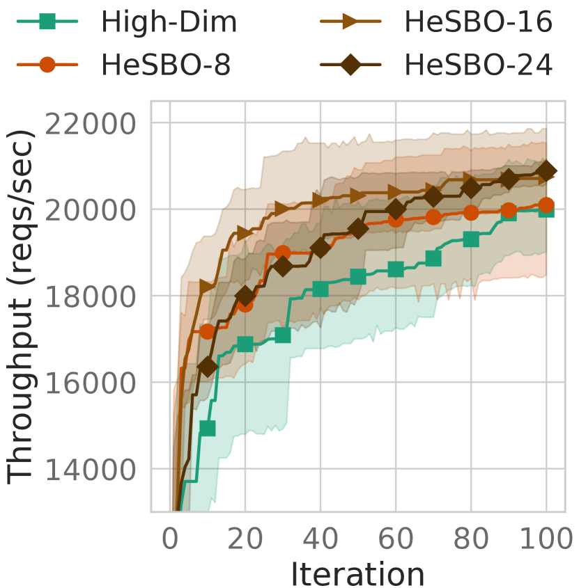
Figure 3. HeSBO ($d=8,16,24$)

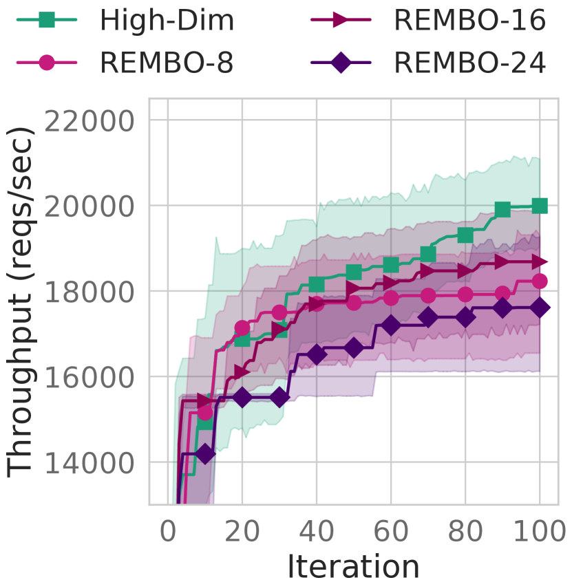
Figure 4. REMBO ($d=8,16,24$)

Figure 3. Best throughput on YCSB-A, when using SMAC to optimize a low-dimensional space from REMBO or HeSBO projections. Baseline (green line) tunes the original space. Shaded areas correspond to $95\%$ confidence interval ranges.⁴

.

HeSBO. To alleviate this drawback, researchers proposed HeSBO (i.e., Hashing-enhanced Subspace BO) (Nayebi et al., 2019), a random linear projection variant that avoids clipping. HeSBO draws inspiration from hashing and sketching to construct its mapping. Assuming an original $D$-dimensional search space $X_{D}$ and given as an input the target dimension $d$, HeSBO first defines a $d$-dimensional search space $X_{d}=[-1,1]^{d}$. Then, it generates a random projection matrix $\mathbf{A}\in\mathbb{R}^{D~{}\times~{}d}$, such that each row contains exactly one non-zero element in a random column that is set to $\pm 1$; the index of the column and the sign of the value are sampled uniformly at random. It does so, using two uniform hashing functions: $h$ that chooses the non-zero entry for each dimension of $X_{D}$, and $\sigma$ that determines the sign of this entry. Intuitively, $\mathbf{A}$ defines an instance of count-sketch projection (Charikar et al., 2002), which is able to adequately preserve the characteristics (i.e., pairwise point distances) of the original high-dimensional space for up to $d$ (important) dimensions (Nayebi et al., 2019).

HeSBO, as expressed by $\mathbf{A}$, provides an one-to-many mapping. Every original knob $i$ in $X_{D}$ is controlled by exactly one synthetic knob $j$ in $X_{d}$, while each synthetic knob can control multiple original ones. Thus, it is impossible for any projection to fall outside of $X_{D}$. This enables HeSBO to perform better than REMBO, especially when high-performing points are in the interior of $X_{D}$ (Letham et al., 2020; Nayebi et al., 2019).

3.3. BO with Random Projections

Integrating either REMBO or HeSBO in the original BO algorithm requires minimal changes. Algorithm 1 describes the modified version and highlights the main differences compared to the “vanilla” high-dimensional BO algorithm. The user provides $d$, the number of dimensions of the low dimensional space. Ideally, this number should be an estimate of the number of important knobs of the DBMS (we discuss how to choose this later). The user also provides $n_{init}$, the number of initial random samples to be generated, as well as $N_{iters}$, the number of iterations to perform (time budget). Reasonable defaults can also be provided based on prior studies.

At first, the projection matrix $\mathbf{A}$ is generated randomly, as described in the previous paragraphs. Note that this matrix $\mathbf{A}$ is computed only once, and remains constant for the entire duration of the optimization process. Then, given $n_{init}$, a space-filling sampling method (e.g., LHS) is employed that generates an initial set of points $p\in X_{d}$. Since these points belong to the approximated space $X_{d}$, they are first projected to $X_{D}$ and then clipped (if using REMBO). For each projected (and possibly clipped) point, the corresponding objective function is computed (i.e., workload is run). Once all initial points have been evaluated, the points and the respective objective function values are used to initialize the surrogate model.

Now, the BO surrogate model can guide the optimization process. Initially, the model suggests a candidate point $p\in X_{d}$ that maximizes the value of the acquisition function. Recall from earlier that the acquisition function tries to propose points that either can provide knowledge about unknown regions (i.e., exploration), or improve the knowledge of already-found good regions, by exploring nearby regions (i.e., exploitation). The suggested point is then projected (and possibly clipped) to $X_{D}$, as before. Finally, the objective function is evaluated at that point, and the surrogate model parameters are updated using the new observation. The above process is repeated, until we exhaust the given number of iterations.

Converting Points to DBMS Knob Values. So far, we assumed that both REMBO and HeSBO project the point suggested by the BO method to the uniform high-dimensional space $X_{D}=[-1,1]^{D}$. However, in reality a DBMS configuration knob space is much more heterogeneous compared to $X_{D}$. Usually, a DBMS configuration space consists of many knobs of different types, like numerical or categorical. The former receive values from a $[min,max]$ range of valid values, while the latter from a predefined list of choices (e.g., on, off). Because the $[min,max]$ range of values (or the number of choices) can significantly vary across different knobs (Van Aken et al., 2017), we need to make sure that $[-1,1]$ values are properly converted to meaningful values for the DBMS knobs.

To achieve this, we employ min-max uniform scaling. In general, to translate a value $x\in[x_{min},x_{max}]$ to a value $y\in[y_{min},y_{max}]$, the following formula is used: $y=y_{min}+\frac{x-x_{min}}{x_{max}-x_{min}}(y_{max}-y_{min})$. Hence, for numerical knobs, we uniformly scale the projected value $x\in[-1,1]$ to the respective $[min,max]$ range, of each knob. If a numerical knob takes discrete values, we further round the scaled value to the correct integer value. For categorical knobs,we perform a two-step conversion process. We first rescale the projected value $x\in[-1,1]$ to a value $y\in[0,1]$, and then we split this range equally to as many bins, as is the number of different choices. The final categorical knob value is defined by which bin the value $y$ falls into.

3.4. Dimensionality of the Projected Space

The only additional input for using these low dimensional projection methods is the number dimensions $d$. Given that the objective function is unknown, it is usually not trivial to provide a good value for $d$. Fortunately, the DBMS knob configuration tuning problem has been studied extensively, and we can rely on observations of past works to provide a good estimate for $d$ (Van Aken et al., 2021; Zhang et al., 2021a; Kanellis et al., 2020).

Prior works have shown good performance improvements when tuning around the $10$-$20\%$ most important, of all knobs considered for tuning. For instance, in (Kanellis et al., 2020) the authors consider a subset of $30$ knobs for PostgreSQL v9.6, and show that tuning the $5$ most important ones ($\approx 17\%$) can yield near-optimal performance. Similarly, prior work (Van Aken et al., 2021) in tuning Oracle v12.2 used a set of 10-40 hand-chosen knobs and (Zhang et al., 2021a) showed that tuning the top-$20$, out of $197$ knobs ($\approx 10\%$) was sufficient for MySQL v5.7. Since the total number of knobs we consider for PostgreSQL v9.6 is $90$, we consider $d$ to be in the range of $[8,16]$. However, as we show next, setting $d$ to an even higher value (i.e., $>16$) is not detrimental to the optimizer performance.

Case Study. We perform a case study using YCSB-A. Our goal is two-fold. First, we want to evaluate how effective REMBO and HeSBO methods are at finding a good projection of the original DBMS configuration space, which can result in better performance. Second, we want to explore how much our selection of $d$ influences the optimizer performance. Our setup consists of tuning $90$ knobs of PostgreSQL v9.6 for $100$ iterations (first $10$ are LHS-generated samples) targeting maximum throughput using SMAC (more setup details in Section 6). We experiment with both REMBO and HeSBO, where we set $d$ to $8$, $16$, or $24$ dimensions.

Figure 3 shows the best throughput achieved at each iteration. Overall, we observe that HeSBO manages to outperform the baseline for all values of $d$, while REMBO is not able to match that performance. REMBO finishes the tuning session with a final configuration that achieves $10$-$15\%$ worse than the baseline. We find that this is because most of the low-dimensional points are clipped during projection to the original DBMS configuration space, which makes it impossible for the optimizer to explore the interior points.

On the other hand, HeSBO does not suffer from the aforementioned issue and performs much better for all values of $d$. This shows that HeSBO can effectively project the original space to a smaller one that is easier to explore, while also retaining many points that achieve good performance. Moreover, we see that $d$ does not greatly affect the quality of the projected space. Even though the $16$-dimensional HeSBO performs the best, all three manage to end up with similar- or better- performing configurations (within $5\%$) at the end of the tuning session, while also converging much faster. This highlights the robustness of HeSBO, and means that we can provide a reasonable estimate of the number of important knobs, rather than an exact number. For the remainder of the paper, we use a $16$-dimensional HeSBO projection for our experiments.

4. Not All Knob Values Are Equal

Shrinking the search space by reducing the number of dimensions stemmed from our prior knowledge of a few important knobs affecting the DBMS performance. We next discuss how auto tuning frameworks can take advantage of another DBMS specific observation: not all knob values have the same performance semantics.

4.1. Special Knob Values in Databases

Table 2. Three examples of hybrid knobs found in PostgreSQL; Each special value performs a different action each time.

Knob name	Range	Short Description	Special Value Action
backend_flush_after	$[0,256]$	Number of pages after which previously performed writes are flushed to disk.	If set to 0, the forced writeback is disabled.
geqo_pool_size	$[0,2^{32})$	Controls the pool size used by GEQO, that is the number of individuals in the genetic population.	If set to 0, then a suitable value is chosen based on geqo_effort and the number of tables in the query.
wal_buffers	$[-1,2^{18})$	Sets the number of disk-page buffers in shared memory for WAL	If set to -1, a size equal to $\mathbf{1/32}$nd of shared_buffers is selected ($\geq 64$kB, not more than one WAL segment).

The configuration search space of a DBMS is heterogeneous, and consists of numerical and categorical knobs. Categorical knobs are inherently different from numerical ones: they enable (or disable) some internal functionality of a component, or select mutually exclusive algorithms for a task. For example, PostgreSQL exposes a plethora of such knobs (e.g., enable_sort, enable_nestloop etc.) (PostgreSQL Documentation, 2022). Choosing different values for a categorical knob may result in substantial DBMS performance variations. Hence, most efficient BO methods treat each categorical knob value independently and make no assumptions regarding their order (Zhang et al., 2021a; Hutter et al., 2011).

On the other hand, the values of numerical knobs have a natural order, which is actively exploited by the BO methods when performing local search. In particular, when the optimizer has identified a good-performing configuration (point), it often opts to explore the nearby regions in order to improve the current optimum (Shahriari et al., 2015). However we find, in practice, some numerical knobs do have special values (e.g., $-1$, $0$) that inevitably break this natural order (Pavlo et al., 2021). We term these knobs as hybrid knobs. If such a knob is set to its special value, it does something very different compared to what it normally does (e.g., disables some feature). Otherwise, it behaves as a regular numerical knob where it sets some underlying functionality of the respective component (e.g., buffer size, flush delays, etc.).

We identified $17$ hybrid knobs for PostgreSQL v9.6 ($24$ exist for PostgreSQL v13.6) from the official documentation (PostgreSQL Documentation, 2022); special values are explicitly mentioned in the knob description. Interestingly enough, for about half of the hybrid knobs, the special value is used in the default configuration.  Table 2 shows some interesting examples. In general, most common behaviors related to special values include (i) disabling some feature, (ii) inferring this knob’s value based on some other’s knob, or (iii) setting this knob’s value using an internal heuristic (or to a predefined value). It is worth noting that the existence of hybrid knobs is neither limited to this specific PostgreSQL version, nor to this DBMS alone. Other popular systems like MySQL (MySQL v8.0 Documentation, 2022), Apache Cassandra (Apache Cassandra Documentation, 2022) and even the Linux kernel (Documentation for /proc/sys/kernel/, 2022; Documentation for /proc/sys/fs/, 2022) also expose similar knobs in their configuration.

Special values make the modeling of the DBMS performance more difficult because they represent a discontinuity in objective function output relative to its input. Figure 5 shows such an example for PostgreSQL’s backend_flush_after knob, when executing a read-heavy YCSB workload: YCSB-B. Typically, larger values for this knob translates to allowing more bytes to remain in kernel page cache, before issuing a writeback request. A value of “$0$” (red diamond in the figure), however, disables the writeback mechanism altogether, resulting in far higher throughput for this workload. From the performance numbers in this figure, we can also deduce the following: if the optimizer tuning this knob lacked the knowledge about the special meaning of value $0$, it would be unlikely that it would ever choose this value during tuning. That is because $0$ is located near the worse-performing values (i.e., 1-10). Instead, the optimizer would focus on exploring the “neighborhood” of larger values for this knob, which seem more promising. Another example is when the number of possible values for a hybrid knob is very large; in this case, it is unlikely that the special value will be among the initial set of random values used to bootstrap the optimizer. For example, assuming an initial set of $10$ uniformly sampled points, the probability of the special value being chosen at least once for the aforementioned backend_flush_after knob is less than $4\%$ .

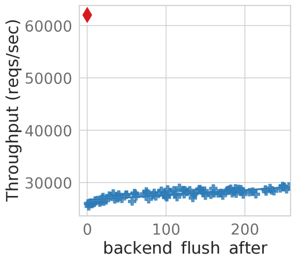
Figure 4. Effect on perf. of special value “$0$”.

BO Suggests

Value $\in$[0,MAX]

Scale to [0,1]

Apply Special

Value Bias $p$

Final Value

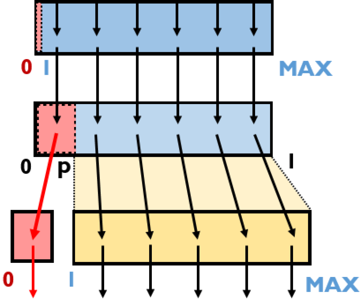
Figure 5. Applying bias to special value “$0$” of a hybrid knob.

Biasing Special Value Sampling Probability We propose a methodology that enables the optimizer to observe the effect of a special value early on in the tuning process. Our key idea is to change the hybrid knobs values proposed, such that we bias the probability of the special value being evaluated. To do this we associate a fixed probability ($p$) for sampling a special value before we begin tuning. To simplify our design, we keep the same probability $p$ for all hybrid knobs we tune. Figure 5 illustrates this process for a single hybrid knob that takes values in $[0,max]$ range, where “$0$” is the special value. Initially, a value $v\in[0,max]$ for this knob is suggested by the optimizer, or through random search. Given this value $v$, we then uniformly scale it to the $[0,1]$ range (using the scaling method described in Section 3.3). If this scaled value is the range $[0,p)$, then we set the resulting knob value $v$ to the special value (i.e., $v$= 0), instead. Otherwise, we uniformly scale it back to the original, minus the special value, range (i.e., $[1,max]$). Finally, the resulting value is used at the DBMS configuration to be evaluated. Note that this methodology requires no modifications to the underlying optimizer, as it only takes place after a certain suggestion is made; thus it can be combined with any optimizer. Furthermore, an extension for hybrid knobs with multiple special values is straightforward: we can define multiple $p_{i}$ (possibly equal with each other), where each one biases exactly one special value.

Choosing the Amount of Bias. Evaluating the impact of the special value early on in the tuning session can help improve total tuning time. Any existent performance anomalies caused by special values can be discovered and the optimizer can then leverage this knowledge. While it might be tempting to construct a configuration consisting solely of special values, and evaluate its performance immediately, this would not help, as all potential anomalies may happen simultaneously. Thus, even if there exists a significant performance improvement from one special value, the optimizer might not be able to attribute this gain. Alternatively, allocating an iteration to measure the effect of every special value independently, may be sub-optimal, especially if the number of such knobs is large.

Suppose the initial set of random configurations consists of $n_{init}$ samples and we set the amount of bias as $p$, the number of samples that evaluate the special value follows a binomial distribution $B(n_{init},p)$. By default, we choose this probability as 20% as it leads to a $\sim$90% confidence level of evaluating the special value (at least once) in the initial set of random configurations. A nice property of this method is that it is invariant to the number of hybrid knobs that are tuned. Users can also alter the value based on their preference.

Two things are worth noting before finishing our discussion regarding hybrid knobs. First, even with a reasonably high confidence level, it is possible that a special value for a knob may not be evaluated during the initial iterations. However, random configurations that are typically proposed by the optimizer periodically (e.g., every $n$-th iterations) are also biased towards each hybrid knobs’ special value and this also handles any undesirable interactions across special values of different knobs. Second, the special value bias does not obstruct the optimizer in any way when it performs local search. Regardless of whether a special value improves performance or not, the optimizer is still able to fine-tune already-evaluated configurations to further improve performance.

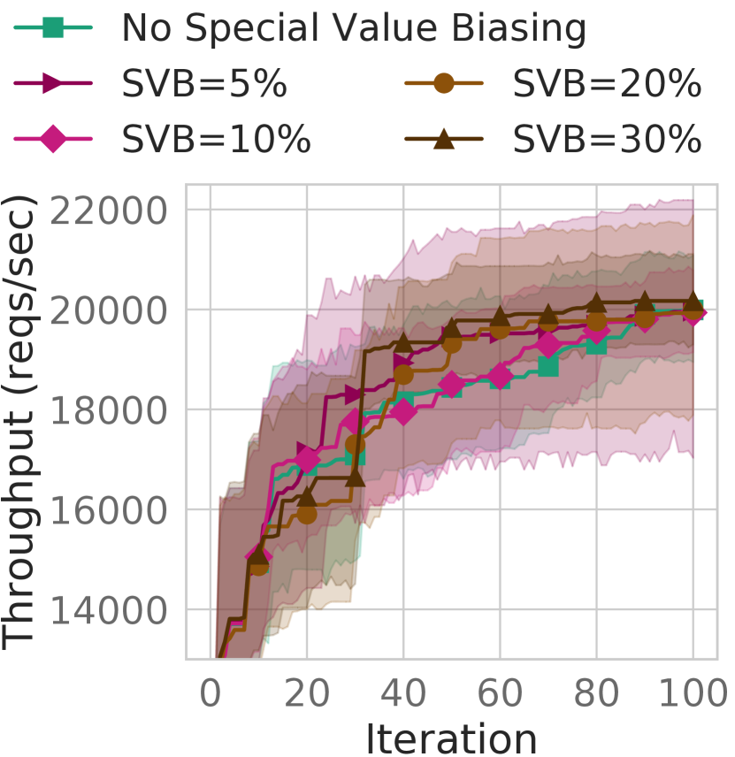
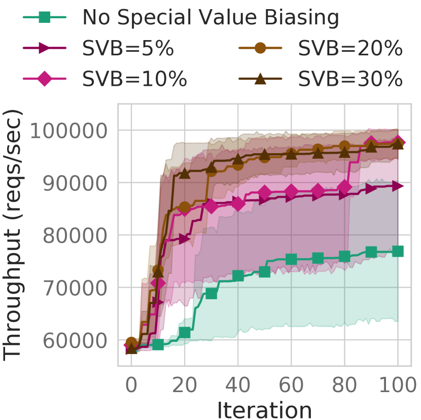
Figure 6. Best performance achieved for YCSB-A (left plot) and YCSB-B (right plot) when applying special value biasing to hybrid knobs (top-left is better).⁴

Case Study. We conduct an experiment with two workloads, YCSB-A, YCSB-B, in order to explore the impact of special value biasing to the performance of the optimizer. We use the same setup used in the case study of Section 3.4 (PostgreSQL v9.6, SMAC, $10$ LHS-generated initial samples), and we vary the bias percentage from $5\%$ to $30\%$. Figure 6 shows the best throughput reached at each iteration. We observe that while for YCSB-A special value biasing does not provide any measurable gains, for YCSB-B the gains are large and increase with the amount of biasing applied up to $20\%$. For the rest of the paper we use a $20\%$ bias percentage.

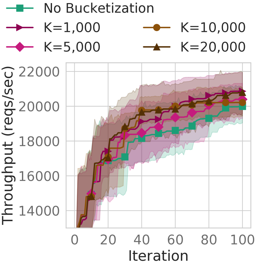
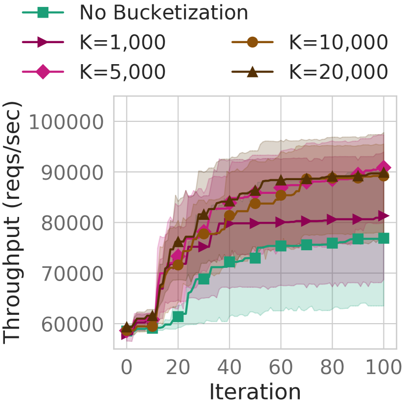
Figure 7. Best performance achieved for YCSB-A (left plot) and YCSB-B (right plot) when tuning the bucketized space vs. the original space (top-left is better).⁴

4.2. Configuration Space Bucketization

Table 3. Examples of discrete knobs with large value range for PostgreSQL v9.6

Knob name	Value Range	Step	Short description
commit_delay	[0, 100000]	$1\mu$s	Sets the delay in microseconds between transaction commit and flushing WAL to disk
max_files_per_process	[25, 50000∗]	1	Sets the maximum number of simultaneously open files for each server process
shared_buffers	[128kB, 16GB∗]	8kB	Sets the amount of memory the database server uses for shared memory buffers
wal_writer_flush_after	[8kB, 16GB∗]	8kB	Amount of WAL written out by WAL writer that triggers a flush

^∗The upper bound value for this knob is infinite, but we pruned it down to this more reasonable value.

Table 4. Workload Properties

Workload	# Tables (# Columns)	RO Txns
YCSB-A	1 (11)	50%
YCSB-B	1 (11)	95%
TPC-C	9 (92)	8%
SEATS	10 (189)	45%
Twitter	5 (18)	1%
RS	4 (23)	33%

While biased sampling of special values can improve the exploration phase of the optimizer, we next look at how discrete configuration knobs in DBMS’ can affect the exploitation (or local search) phase.

Discrete configuration knobs exposed by the DBMS can have very dissimilar ranges. Some knobs have $10$ possible values while others range in millions. A broader range of values gives more fine-grained control of the underlying mechanism. Table 3 lists some knobs in PostgreSQL that have a large number of unique values. One example is shared_buffers, which specifies the size of in-memory shared buffers at the granularity of a single page. Another example is commit_delay, which controls the delay before a committed transaction is flushed to disk; this delay can be set at microseconds granularity. Again, the existence of knobs with such characteristics is not restricted to PostgreSQL (Apache Cassandra Documentation, 2022; MySQL v8.0 Documentation, 2022).

While having many different choices for knob values enables fine-grained control, it greatly increases the size of the configuration search space. We observe that for many configuration knobs with large values ranges, small changes are unlikely to affect the DBMS performance significantly. For instance, when tuning the value of commit_delay, the performance is similar for $10,000\mu s$ and $10,100\mu s$ (i.e., adding $0.1ms$). Based on this observation, we explore bucketizing the knob value space at fixed intervals. We can do this by limiting the number of unique values that any configuration knob can take to $K$. Knobs with more than $K$ values are rounded down to use only $K$ unique values; these new values are uniformly spread across the entire range (i.e., if $K=100$ for commit_delay, the new set of discrete values will be 0, 1000, 2000 … 100000). Knobs with less than $K$ values remain unaffected, and are tuned as before.

Case Study. We use a simple policy to set $K$ and explore the effect of bucketizing. We chose the same $K$ for all knobs as it is hard to know the ideal value without performing expensive offline profiling. We set $K$ based on the distribution of the ranges of values such that the number of knobs to be bucketized is $P\%$ of all knobs.

We run an experiment with YCSB-A, YCSB-B workloads and compare SMAC’s performance when tuning a bucketized space to tuning the original configuration space, for different values of $K$ (from $1,000$ to $20,000$). Figures 7 shows the best throughput reached at each iteration. For YCSB-A, while the performance in the first $20$ iterations is similar, in later iterations the bucketized (smaller) space reaches a better-performing configuration faster (for most values of $K$). For YCSB-B we see larger benefits starting at iteration 10 (especially for $K\geq 5,000$). Thus, we see that the benefits from bucketization varies across workloads. In the future, we plan to better understand when BO methods benefit from using bucketization, especially given prior work in ML (Bergstra and Bengio, 2012) has shown the pitfalls of using a fixed grid for hyperparameter optimization. For the rest of this paper we set $K=10,000$ (i.e., from $P\%=50\%$).

5. LlamaTune Design

So far, we have presented three DBMS specific observations that can improve the configuration optimizer: (i) random low-dimensional projections, (ii) biasing the special value of hybrid knobs, and (iii) bucketization for knobs with many unique values. We next present LlamaTune, a unified design that incorporates these approaches.

A unified design should satisfy three main requirements. First, the optimizer should always operate on the low-dimensional space, and not in the original DBMS knob configuration one. Second, the special value biasing should be performed only over the set of hybrid knobs. Otherwise, we might unnecessarily skew the values of other knobs towards non-existent special value(s). Finally, the bucketized value space for the set of knobs should be exposed to the optimizer, so it is aware of the larger sampling intervals; otherwise it will still continue to sample at finer granularities.

In our attempt to meet the above design requirements, we devise a unified tuning pipeline (LlamaTune) that employs a bucketized version of the low-dimensional search space, and applies the special value biasing only after a point has been suggested. Instead of the original low-dimensional continuous space $X_{D}=[-1,1]^{D}$, we define a bucketized search space $X_{D}^{\prime}$, similar to $X_{D}$, but with the ability to sample values only at fixed intervals, as defined by the number of maximum unique values (i.e., $K$). Exposing the space $X_{D}^{\prime}$ to the optimizer satisfies the first, but only partly the third requirement (we explain more below). The second requirement is satisfied by applying the special value bias after the point has been projected to the original space, but before the values are re-scaled. This way, the biasing approach does not interfere with the internals of the random projection method. The main limitation of this design is that bucketizing the entire search space may affect fine tuning of continuous knobs. However, we believe that the performance gains of optimizing a smaller space outweighs this drawback in most cases, especially when we use a conservative value for $K$.

Example: In Figure 8, we present an example of our design. We consider a scenario where we tune five DBMS knobs using a $2$-dimensional random projection derived by HeSBO. We set the special value bias to $20\%$, and bucketize the low-dimensional space to $K=10,000$. Among these knobs, commit_delay is a discrete knob, geqo_selection_bias is continuous knob, and enable_seqscan is a binary categorical knob. The remaining two knobs are hybrid knobs: backend_flush_after has a special value of “$0$”; for wal_buffers it is “$-1$”.

Initially, the optimizer suggests a point $[-0.8,0.4]$ that belongs to the low-dim $[-1,1]^{d}$ bucketized space. The value $Q$ denotes the size of the fixed interval (i.e., $2/K$). This point is then projected to a high-dimensional point in $[-1,1]^{D}$ (i.e., $D=5$). The first synthetic knob is mapped to both hybrid knobs (but with opposite $\pm$ signs), while the second one maps to the remaining three. The projected point now corresponds to a real DBMS knob configuration. Next, we normalize all knob values to $[0,1]$, and apply special value biasing only for the two hybrid knob values. Here, backend_flush_after’s original value of $0.1$ has been biased towards its special value $0$ (i.e., inside the $[0,0.2)$ range), while wal_buffers has been scaled (i.e., inside the $[0.2,1]$ range) to compensate for the $20\%$ special value bias. Finally, all normalized values are converted to the corresponding physical knob values. These values now comprise the DBMS configuration that is evaluated on the real system.

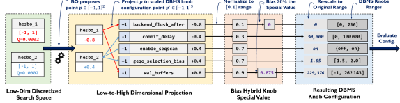
Figure 8. LlamaTune: Tuning example that highlights the unified end-to-end pipeline.

6. Evaluation

In this section, we evaluate LlamaTune on various workloads and show that it can improve the time taken for tuning PostgreSQL on six different workloads by $1.96\times$ up to $11.0\times$ when using SMAC.

6.1. Experiment Setup

Hardware. We conduct our experiments on CloudLab (Duplyakin et al., 2019). Each tuning session runs on a single c220g5 node located at the Wisconsin cluster. The DBMS runs on top of a 10-core Intel Xeon Silver 4114 CPU with 16 GB of RAM and uses a 480 GB SATA SSD. The workload clients and the optimizer algorithm are isolated from the DBMS, and run on a separate CPU (each node has two sockets).

Tuning Settings. We run most experiments with PostgreSQL v9.6, but also use PostgreSQL v13.6. We select a set of tunable 90 knobs that could affect DBMS performance; we exclude from this set all knobs related to debugging, security, and path-setting. We repeat each experiment five times using different random seeds as input to our optimizer; we report the mean best performance from all runs. Each tuning session consists of $100$ iterations , and each run consists of five minutes of running the workload. For most experiments we optimize for overall system throughput (i.e., higher is better); we also show that our approach can yield gains when optimizing for $95$-th percentile latency. The configurations of the first $10$ iterations are generated randomly using LHS (McKay et al., 1979). For those configurations that cause the DBMS to crash, we assign one fourth of the worst throughput we have seen so far to that iteration; initially this value is set to the performance of the default configuration. The above tuning configuration is similar to prior works (Zhang et al., 2021a; Van Aken et al., 2021; Van Aken et al., 2017).

Table 5. Perf. gains of LlamaTune when coupled with SMAC. We report average and $\mathbf{[5\%,95\%]}$ confidence interval numbers.

Workload	Final Throughput Improvement		Time-to-Optimal Speedup
	Average	[5%, 95%] CI	Average	[5%, 95%] CI
YCSB-A	2.74%	[0.9%, 4.5%]	1.96x [51 iter]	[1.1x, 3.3x]
YCSB-B	20.85%	[10.2%, 27.9%]	5.5x [18 iter]	[1.2x, 33.0x]
TPC-C	6.30%	[-0.3%, 12.4%]	11.0x [9 iter]	[1.0x, 14.1x]
SEATS	7.45%	[2.4%, 11.7%]	6.67x [15 iter]	[1.8x, 12.5x]
Twitter	4.38%	[1.7%, 6.8%]	6.62x [13 iter]	[5.4x, 8.6x]
RS	1.08%	[0.2%, 1.9%]	1.98x [49 iter]	[1.1x, 3.1x]

Workloads. For our experiments, we use six OLTP workloads with different characteristics (shown in Table 4). We use the official YCSB suite (Cooper et al., 2010), and BenchBase (formerly OLTP-Bench (Difallah et al., 2013)). We use two workloads variants from the YCSB suite: the read-write ($50\%$-$50\%$) balanced YCSB-A, and the read-heavy ($95\%$ read, $5\%$ write), YCSB-B. YCSB workloads perform simple random access key queries, on a single $10$-column table, based on a Zipfian distribution. From BenchBase, we use the TPC-C, SEATS, Twitter, and ResourceStresser (RS) workloads. Both TPC-C and SEATS are traditional OLTP workloads with multiple tables, and complex relations. TPC-C consists of five (mostly write-heavy) transactions that operate on nine tables, and simulates an order processing system for a warehouse. SEATS resembles the back-end system of an airline ticketing service using ten tables and six transaction types. Twitter is a web-oriented workload that uses public traces to simulate the core functionality of a micro-blogging application; it consists of five tables and five heavily-skewed transaction types. RS is a synthetic workload with the intention to introduce independent contention on different resources (i.e., CPU, disk I/O and locks) (Difallah et al., 2013). We employ $40$ clients, and select the scale factor of all workloads accordingly, so that all databases are $20$GB. In the future, we also plan to evaluate LlamaTune’s set of techniques with OLAP workloads.

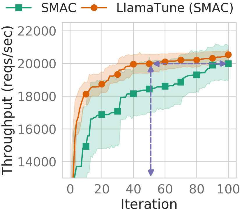
Figure 9. (a) YCSB-A

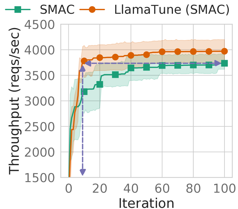
Figure 10. (b) TPC-C

Figure 11. (c) Twitter

Figure 9. Best throughput achieved by LlamaTune. Time-to-optimal also shown.⁴

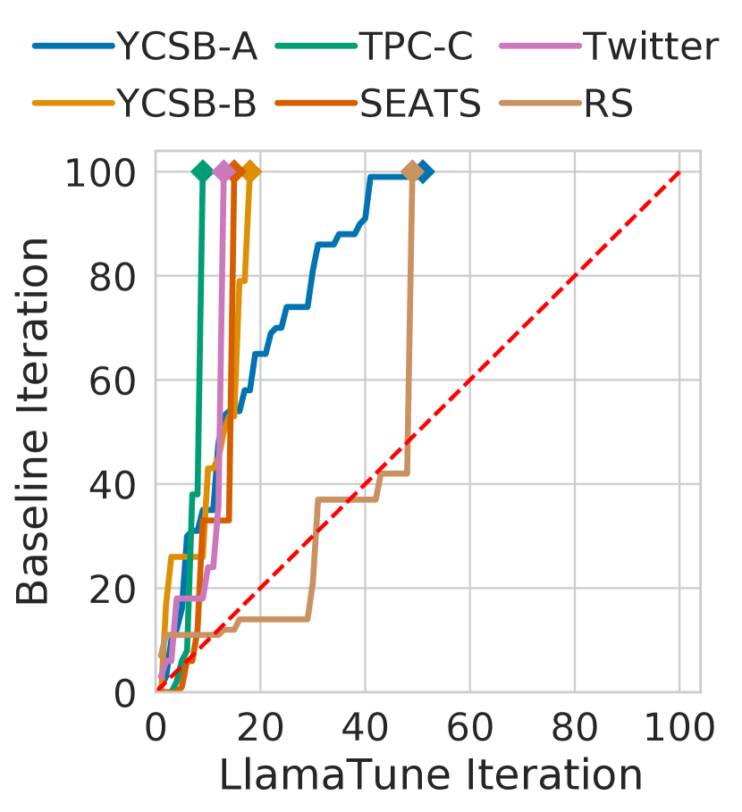
Figure 10. LlamaTune convergence gains vs. SMAC.

Optimizers. For our experiments we use three state-of-the-art optimizers: SMAC, GP-BO, and DDPG. All three are shown to outperform alternative methods in most cases (Zhang et al., 2021a). For SMAC we use the implementation provided by the authors (Lindauer et al., 2021), while for the GP-BO we leverage OpenBox’s (Li et al., 2021) implementation, also used in prior work (Zhang et al., 2021a). For DDPG, we implement the original neural network architecture used in CDBTune (Zhang et al., 2019) with PyTorch (Paszke et al., 2019).

LlamaTune Implementation. Since LlamaTune is agnostic to the underlying optimizer, we implement it in Python3 with $800$ LOCs on top of all three optimizers. In the experiments, LlamaTune uses HeSBO random projections with $d=16$ dimensions, sets the special value biasing to $20\%$, and bucketizes the search space to limit the number of unique values of each dimension to $K=10,000$.

Evaluation Metrics. We use two metrics to evaluate the performance of LlamaTune: final DBMS throughput (latency) improvement, and time-to-optimal throughput (latency). The former is related to the difference in performance (e.g., throughput, $95$th $\%$-tile latency) of the best-performing configurations found at the end of tuning (i.e., after 100 iterations). We compare the performance improvement (in $\%$) realized by LlamaTune compared to the baseline. The latter is inspired from a popular metric used in ML (i.e., time-to-accuracy) that quantifies the time taken by ML algorithms to reach a certain accuracy level (Coleman et al., 2019). We report the earliest iteration at which LlamaTune has found a better-performing configuration compared to the baseline optimal, as well as the relative speedup.

6.2. Efficiency Evaluation

Table 6. Perf. gains of LlamaTune when coupled with SMAC, and tuning for $95$-th percentile tail latency.

Workload	Final 95th %-tile Latency Reduction		Time-to-Optimal Speedup
	Average	[5%, 95%] CI	Average	[5%, 95%] CI
TPC-C	14.56%	[-1.1%, 30.8%]	2.14x [43 iter]	[0.9x, 18.4x]
SEATS	11.16%	[1.3%, 21.2%]	2.35x [34 iter]	[1.2x, 4.7x]
Twitter	3.33%	[-3.9%, 10.9%]	1.38x [68 iter]	[0.9x, 3.4x,]

Table 7. Perf. gains of LlamaTune when coupled with SMAC, and tuning the newer DBMS, PostgreSQL v13.6.

Workload	Final Throughput Improvement		Time-to-Optimal Speedup
	Average	[5%, 95%] CI	Average	[5%, 95%] CI
YCSB-A	10.73%	[8.9%, 13.0%]	2.69x [36 iter]	[2.1x, 7.5x]
YCSB-B	3.63%	[2.3%, 4.9%]	2.54x [37 iter]	[1.4x, 3.9x]
TPC-C	2.91%	[1.1%, 4.2%]	1.56x [63 iter]	[1.4x, 4.3x]
SEATS	20.25%	[16.7%, 23.5%]	6.0x [16 iter]	[3.4x, 16.0x]
Twitter	2.61%	[0.8%, 4.3%]	8.25x [12 iter]	[5.2x, 12.4x]
RS	0.69%	[0.0%, 1.4%]	2.12x [42 iter]	[0.9x, 4.1x]

In this section, we evaluate the tuning efficiency of LlamaTune while using the vanilla SMAC optimizer as our baseline.

Optimizing for Throughput. We set the optimizer target to throughput; Table 5 shows the results for all six workloads. We make two observations. First, LlamaTune reaches the performance of the baseline SMAC optimum configuration by $\sim 5.62\times$ faster on average. For four of the total six workloads, it reaches that performance before iteration $20$, which highlights its increased sample-efficiency. Second, LlamaTune can improve the average final throughput (after $100$ iterations) on all workloads, by $\sim 7.13\%$ on average, compared to vanilla SMAC (from $1.08\%$ better on RS to $20.85\%$ better on YCSB-B). Both TPC-C, SEATS, which are complex OLTP workloads show consistent gains of $6$-$7\%$, while Twitter which has vastly different characteristics, also performs well. The synthetic RS workload is particularly hard to optimize, as the overall performance gains compared to the default configuration is only around $10\%$; this explains why LlamaTune’s improvement is small, compared to the other workloads.

Figure 10 shows the best performance convergence curve for three workloads: YCSB-A, TPC-C, and Twitter. The red line indicates the earliest iteration of LlamaTune that results in better performance compared to the baseline (i.e., time-to-optimal). The contributing factors for the improvement include projection to a low-dimensional space, as well as special value biasing, which accelerates exploring their effect on performance. We also observe that for YCSB-A, LlamaTune reduces the variance across different runs, making it more likely for any run to realize the highest gains.

Figure 10 shows the mean improvement of LlamaTune over the baseline (SMAC) during the entire tuning session. For every iteration of LlamaTune (x-axis), we plot the earliest iteration at which SMAC achieves the same (or better) performance on the (y-axis); the point at which LlamaTune surpasses the best SMAC performance is indicated by a diamond. We see that for all workloads other than RS, LlamaTune provides improvements over SMAC across all iterations. For RS, we see that LlamaTune performs better from around iteration 30. Overall, we can see that given any fixed iteration budget, LlamaTune can provide meaningful speedups across workloads.

Optimizing for Tail Latency. Now, we experiment with a different tuning scenario, where we aim to reduce the $95$-th percentile latency, at a fixed rate of incoming requests. We experiment with three workloads from the BenchBase suite: TPC-C, SEATS, and Twitter. We set the rate of incoming requests to half of the best throughput achieved from the previous experiments: $2,000$ requests per second for TPC-C, $8,000$ for SEATS, and $60,000$ for Twitter. Table 6 summarizes the results. We observe that LlamaTune outperforms the baseline SMAC on all three workloads. On average LlamaTune yields a $\sim 1.96\times$ time-to-optimal speedup, and $\sim 9.68\%$ better final tail latency. These results indicate that our tuning pipeline is still effective in more complicated tuning targets.

Figure 11. (a) YCSB-A

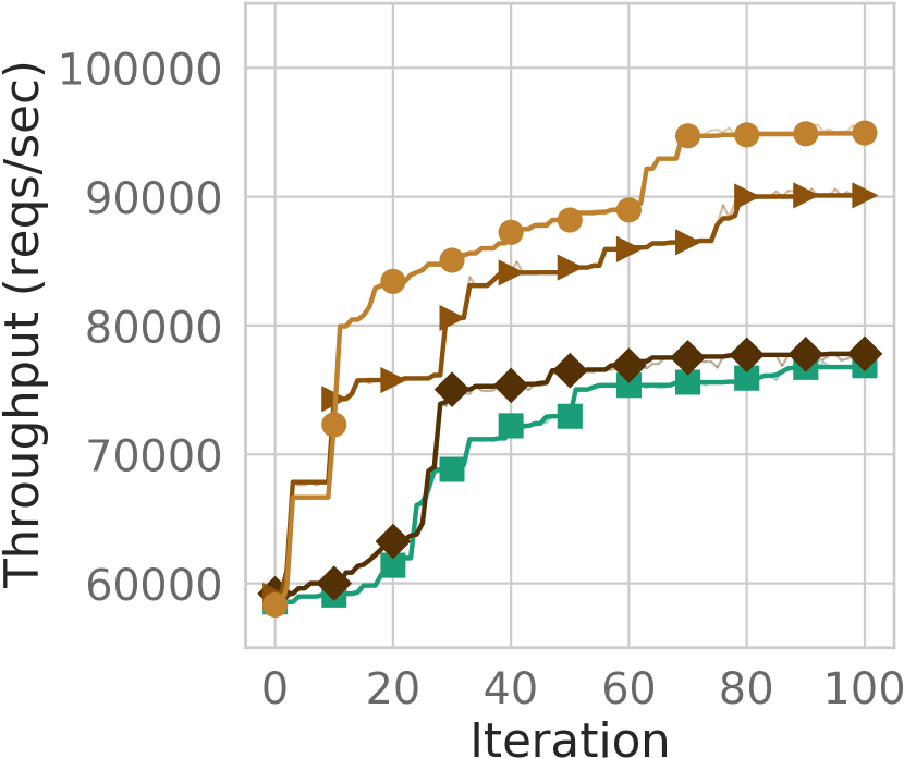
Figure 12. (b) YCSB-B

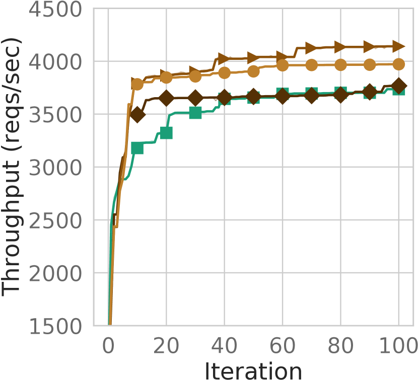
Figure 13. (c) TPC-C

Figure 11. Ablation study for the three components of LlamaTune.⁴

Table 8. Performance gains of LlamaTune when coupled with a different BO-based method, GP-BO.

Workload	Final Throughput Improvement		Time-to-Optimal Speedup
	Average	[5%, 95%] CI	Average	[5%, 95%] CI
YCSB-A	1.10%	[-3.1%, 6.1%]	1.11x [90 iter]	[0.8x, 3.1x]
YCSB-B	21.54%	[10.9%, 33.3%]	19.4x [5 iter]	[8.8x, 32.3x]
TPC-C	18.57%	[10.8%, 26.3%]	10.38x [8 iter]	[4.9x, 16.6x]
SEATS	10.06%	[8.1%, 11.9%]	3.5x [28 iter]	[1.3x, 19.6x]
Twitter	4.28%	[1.4%, 7.1%]	14.83x [6 iter]	[3.4x, 17.8x]
RS	0.50%	[-0.9%, 1.6%]	1.43x [70 iter]	[0.8x, 7.1x]

6.3. Effectiveness on Different DBMS Version

We next experiment with a newer version of PostgreSQL, v13.6, to evaluate LlamaTune’s effectiveness and robustness when the underlying DBMS characteristics change. Compared to the version used throughout the paper (v9.6), this newer version includes several major improvements from just-in-time compilation to better parallel query execution; this is also reflected in the increased number of configuration knobs (PostgreSQL Documentation, 2022). Porting LlamaTune to the new version requires characterizing which of the newly-introduced knobs should be included in the set of tunable knobs, and identifying new hybrid knobs (along with their special value). Overall it took us $\sim 4$ hours to fully integrate LlamaTune with this version. We now tune $112$ knobs ($23$ of which are hybrid ones) using the same hyperparameters for LlamaTune, as before, and we compare against vanilla SMAC; the rest of the setup is identical to section 7. Table 7 shows the results. On average, LlamaTune achieves $\sim 3.86\times$ time-to-optimal speedup, and manages to match or outperform the vanilla SMAC in all cases. Interestingly, we also observe that the recent PostgreSQL improvements affect the gains realized by LlamaTune. For example, with YCSB-B, while LlamaTune achieves similar throughput across Postgres versions, we find that SMAC achieves better throughput with v13.6, narrowing the throughput improvement of LlamaTune over SMAC from 20.8% to 3.6%. On the other hand, we see better throughput improvements with LlamaTune for SEATS and YCSB-A.

6.4. Generalizing across Optimizers

GP-BO. We now change the underlying optimizer of LlamaTune to GP-BO, which uses Gaussian Processes as surrogate model, instead of SMAC’s random forests. We conduct the same set of experiments as section 7, optimizing for maximum throughput. Table 8 shows the results. We observe that LlamaTune again outperforms the vanilla GP-BO optimizer on all six workloads. Across all workloads, the mean time-to-optimal speedup is $\sim 8.4\times$, while LlamaTune also finds better-performing configurations. In particular, we see much faster convergence-to-baseline optimal for YCSB-B ($19.4\times$), TPC-C ($10.38\times$), and Twitter ($14.83\times$) where less than $10$ iterations are required. RS still remains a challenging workload to optimize, as LlamaTune could not improve much over the baseline GP-BO.

Table 9. Perf. gains of LlamaTune when coupled with DDPG.

Workload	Final Throughput Improvement		Time-to-Optimal Speedup
	Average	[5%, 95%] CI	Average	[5%, 95%] CI
YCSB-B	24.95%	[15.85%, 32.69%]	5.17x [18 iter]	[2.38x, 6.64x]
TPC-C	12.24%	[-1.77%, 30.27%]	8.40x [ 5 iter]	[0.82x, 21.0x]
Twitter	2.34%	[-0.60%, 5.14%]	1.18x [66 iter]	[0.75x, 13.0x]
RS	0.71%	[-1.16%, 2.47%]	1.79x [34 iter]	[0.74x, 3.39x]

DDPG. We next evaluate LlamaTune when it is coupled with DDPG, a reinforcement learning-based optimizer (used in CDBTune (Zhang et al., 2019) and QTune (Li et al., 2019)). DDPG leverages two neural networks: the actor that recommends a configuration when given the internal DBMS state (metrics) as input, and the critic that assesses how good each configuration is, based on its resulting performance (reward). We use a similar setup as in  7 and maximize throughput. To represent the internal DBMS state, we sample $27$ system-wide PostgreSQL metrics every $5$ seconds, and feed their average into the neural network at the end of each iteration. Table 9 presents the results for four workloads. On average, LlamaTune achieves a time-to-optimal speedup of $4.14\times$, while also finding better-performing configurations (up to $25\%$ for YCSB-B). Thus, overall we can see that our benefits extend across optimizers.

6.5. Ablation Study

We next conduct an ablation study to better understand the benefits from each of LlamaTune’s components. We compare using only the HeSBO-16 low-dimensional projection, with HeSBO-16 plus special value biasing (SVB), and with the entire LlamaTune pipeline (i.e. with configuration space bucketization). We compare LlamaTune to SMAC on three workloads: YCSB-A, YCSB-B, and TPC-C (Figure 11). We observe that all three combinations perform as well or better compared to the SMAC baseline, for all three workloads. For YCSB-B we see that only using HeSBO-16 achieves $\sim 2\times$ time-to-optimal speedup, while using the other techniques this speedup is improved to $\sim 5.5\times$. For YCSB-A, the plain HeSBO-16 projection performs the best, while it seems that the special value biasing hinders LlamaTune’s convergence; the final throughput is not affected though. This is because special knobs values do not improve the YCSB-A performance, and thus biasing the optimizer sampling towards those, slightly delays exploring other better-performing regions. For TPC-C, we observe that HeSBO-16 and special value biasing have a positive effect on optimization performance. We note a small performance degradation when applying the search space bucketization and believe that this is because of LlamaTune imposing a bucketized space for all knobs, not just for the ones with a large number of unique values. Finally, we note that even though the integration of special value biasing and space bucketization do not always help, their (negative) impact on performance is very limited; when they do, we can realize significant gains.

6.6. Optimizer Overhead

Table 10. Optimizer overhead & LlamaTune improvements

Optimizer	Time Overhead (minutes)		Time Reduction (%)
	Baseline	LlamaTune
SMAC	26.75	3.83	86
GP-BO	256.57	62.95	75
DDPG	0.075	0.066	12

We measure the time taken by the optimizer to suggest the next configuration across the entire tuning session (i.e., $100$ iterations). This time includes updating the underlying surrogate models, as well as comparing the set of possible configuration candidates; it does not include the time for a configuration to be evaluated on the DBMS. Table 10 summarizes the time overhead of LlamaTune compared to the vanilla optimizers. LlamaTune reduces the time overhead by $86\%$, $75\%$, $12\%$ when being integrated with SMAC, GP-BO, and DDPG, respectively. The reduced number of dimensions, resulting from the low-dimensional projection is the primary reason, as the optimizers have to model a much smaller space. This is especially important for the GP-BO optimizer, due to the non-linear sampling behavior of GPs (Shahriari et al., 2015). The time overhead of special values biasing, and knob values bucketization are negligible.

7. Conclusion

In this paper, we studied techniques to improve the sample efficiency of optimizers used in DBMS tuning and showed how we can leverage domain knowledge to perform low dimensional tuning while handling special knob values and large knob value ranges. We empirically showed that our techniques can find good performing configurations up to $11\times$ faster compared to the state-of-the-art optimizer (SMAC), and that our tuning pipeline is robust when tuning for different performance targets, optimizers, and DBMS versions. In the future, we plan to extend our work to other contexts, such as tuning Linux or dataflow engines like Apache Spark.

APPENDIX

Appendix A Deployment Scenario

Table 11. Evaluation for three early-stopping policies. We report mean performance improvement and the iteration when the session was stopped.

Policies	(0.5%, 10)		(1%, 10)		(1%, 20)
Metrics	Perf. Improv (%)	Num Iters	Perf. Improv (%)	Num Iters	Perf. Improv (%)	Num Iters
YCSB-A	-0.01	49	-0.01	46	1.12	71
YCSB-B	11.82	42	11.67	35	20.85	96
TPC-C	3.08	26	3.08	26	6.11	72
SEATS	1.82	31	1.55	25	6.71	76
Twitter	3.76	29	3.76	29	3.82	39
RS	-1.71	26	-2.82	12	0.82	69

We consider a deployment scenario in which the user wishes to tune a database for a new workload. Our goal here is to study how the gains in terms of convergence speed (i.e. time-to-optimal) can be realized in this setting. Specifically, we stop the tuning session early, once we believe that LlamaTune has found a good configuration, thus saving valuable time and resources. Ideally, the DBMS performance at this point will be equal or better than running the vanilla optimizer for a fixed time budget (e.g., 100 iterations).

To this end, we augment LlamaTune with an early-stopping policy used in the ML community (Prechelt, 1998). This policy continuously monitors the best performance achieved at each iteration, and makes a decision on when tuning should be stopped. Formally, it can be expressed by two parameters: the minimum best performance improvement ($x$ in $\%$), and the maximum number of $k$ iterations to wait for this improvement to be made (patience). If $k$ iterations have passed and the aggregate performance improvement is smaller than the one required ($x$), then the session is terminated.

We experiment with three (min-improv, patience) policy configurations on all six workloads. Table 11 shows the final performance improvement over the vanilla SMAC when tuning stops. We first focus on the $(1\%,10)$ early-stopping policy configuration. When using the $(1\%,10)$ early-stopping policy, we see that for most workloads LlamaTune achieves better (up to $11.67\%$ for TPC-C) or equal final performance, compared to the SMAC baseline, while stopping after 29 iterations on average. For RS, the policy terminates very early ($12$th iteration), which results in slight decrease in final throughput. We can alleviate this behavior by choosing a more conservative policy. For instance, reducing the minimum improvement threshold to $0.5\%$ (i.e., left column) results in slight increase in the final throughput for YCSB-B, SEATS, and most notably RS, as the policy makes the decision to stop around $10$ iterations later in the tuning process. Conversely, we can increase the policy patience to $20$ iterations (i.e., right column) to realize near-optimal gains for all workloads, at the expense of spending around $70$ iterations to tune on average. We allow users to adjust the early-stopping policy in order to trade-off between better final performance vs. earliest stopping possible. The above results demonstrate that it is possible to realize LlamaTune’s gains for tuning new DBMS workload deployments.

References

- (1)
- Apache Cassandra Documentation (2022) Apache Cassandra Documentation. 2022. https://cassandra.apache.org/doc/latest/cassandra/configuration/cass_yaml_file.html.
- Bergstra and Bengio (2012) James Bergstra and Yoshua Bengio. 2012. Random Search for Hyper-Parameter Optimization. Journal of Machine Learning Research 13, 10 (2012), 281–305. http://jmlr.org/papers/v13/bergstra12a.html
- Cereda et al. (2021) Stefano Cereda, Stefano Valladares, Paolo Cremonesi, and Stefano Doni. 2021. CGPTuner: a contextual gaussian process bandit approach for the automatic tuning of IT configurations under varying workload conditions. Proceedings of the VLDB Endowment 14, 8 (2021), 1401–1413.
- Charikar et al. (2002) Moses Charikar, Kevin Chen, and Martin Farach-Colton. 2002. Finding frequent items in data streams. In International Colloquium on Automata, Languages, and Programming. Springer, 693–703.
- Coleman et al. (2019) Cody Coleman, Daniel Kang, Deepak Narayanan, Luigi Nardi, Tian Zhao, Jian Zhang, Peter Bailis, Kunle Olukotun, Chris Ré, and Matei Zaharia. 2019. Analysis of dawnbench, a time-to-accuracy machine learning performance benchmark. ACM SIGOPS Operating Systems Review 53, 1 (2019), 14–25.
- Cooper et al. (2010) Brian F. Cooper, Adam Silberstein, Erwin Tam, Raghu Ramakrishnan, and Russell Sears. 2010. Benchmarking Cloud Serving Systems with YCSB. In Proceedings of the 1st ACM Symposium on Cloud Computing (Indianapolis, Indiana, USA) (SoCC ’10). Association for Computing Machinery, New York, NY, USA, 143–154. https://doi.org/10.1145/1807128.1807152
- Dalibard et al. (2017) Valentin Dalibard, Michael Schaarschmidt, and Eiko Yoneki. 2017. BOAT: Building Auto-Tuners with Structured Bayesian Optimization. In Proceedings of the 26th International Conference on World Wide Web (Perth, Australia) (WWW ’17). International World Wide Web Conferences Steering Committee, Republic and Canton of Geneva, CHE, 479–488. https://doi.org/10.1145/3038912.3052662
- Difallah et al. (2013) Djellel Eddine Difallah, Andrew Pavlo, Carlo Curino, and Philippe Cudré-Mauroux. 2013. OLTP-Bench: An Extensible Testbed for Benchmarking Relational Databases. PVLDB 7, 4 (2013), 277–288.
- Documentation for /proc/sys/fs/ (2022) Documentation for /proc/sys/fs/. 2022. https://www.kernel.org/doc/html/latest/admin-guide/sysctl/fs.html#pipe-user-pages-hard.
- Documentation for /proc/sys/kernel/ (2022) Documentation for /proc/sys/kernel/. 2022. https://www.kernel.org/doc/html/latest/admin-guide/sysctl/kernel.html#perf-cpu-time-max-percent.
- Duan et al. (2009) Songyun Duan, Vamsidhar Thummala, and Shivnath Babu. 2009. Tuning database configuration parameters with iTuned. Proceedings of the VLDB Endowment 2, 1 (2009), 1246–1257.
- Duplyakin et al. (2019) Dmitry Duplyakin, Robert Ricci, Aleksander Maricq, Gary Wong, Jonathon Duerig, Eric Eide, Leigh Stoller, Mike Hibler, David Johnson, Kirk Webb, Aditya Akella, Kuangching Wang, Glenn Ricart, Larry Landweber, Chip Elliott, Michael Zink, Emmanuel Cecchet, Snigdhaswin Kar, and Prabodh Mishra. 2019. The Design and Operation of CloudLab. In 2019 USENIX Annual Technical Conference (USENIX ATC 19). USENIX Association, Renton, WA, 1–14. https://www.usenix.org/conference/atc19/presentation/duplyakin
- Eriksson and Jankowiak (2021) David Eriksson and Martin Jankowiak. 2021. High-dimensional Bayesian optimization with sparse axis-aligned subspaces. In Proceedings of the Thirty-Seventh Conference on Uncertainty in Artificial Intelligence (Proceedings of Machine Learning Research), Cassio de Campos and Marloes H. Maathuis (Eds.), Vol. 161. PMLR, 493–503. https://proceedings.mlr.press/v161/eriksson21a.html
- Gur et al. (2021) Yaniv Gur, Dongsheng Yang, Frederik Stalschus, and Berthold Reinwald. 2021. Adaptive Multi-Model Reinforcement Learning for Online Database Tuning. In Proceedings of the 24th International Conference on Extending Database Technology, EDBT 2021, Nicosia, Cyprus, March 23 - 26, 2021, Yannis Velegrakis, Demetris Zeinalipour-Yazti, Panos K. Chrysanthis, and Francesco Guerra (Eds.). OpenProceedings.org, 439–444. https://doi.org/10.5441/002/edbt.2021.48
- Hutter et al. (2011) Frank Hutter, Holger H. Hoos, and Kevin Leyton-Brown. 2011. Sequential Model-Based Optimization for General Algorithm Configuration. In Learning and Intelligent Optimization, Carlos A. Coello Coello (Ed.). Springer Berlin Heidelberg, Berlin, Heidelberg, 507–523.
- Kanellis et al. (2020) Konstantinos Kanellis, Ramnatthan Alagappan, and Shivaram Venkataraman. 2020. Too Many Knobs to Tune? Towards Faster Database Tuning by Pre-Selecting Important Knobs. USENIX Association, USA.
- Letham et al. (2020) Ben Letham, Roberto Calandra, Akshara Rai, and Eytan Bakshy. 2020. Re-examining linear embeddings for high-dimensional bayesian optimization. Advances in neural information processing systems 33 (2020), 1546–1558.
- Li et al. (2019) Guoliang Li, Xuanhe Zhou, Shifu Li, and Bo Gao. 2019. QTune: A Query-Aware Database Tuning System with Deep Reinforcement Learning. Proc. VLDB Endow. 12, 12 (aug 2019), 2118–2130. https://doi.org/10.14778/3352063.3352129
- Li et al. (2021) Yang Li, Yu Shen, Wentao Zhang, Yuanwei Chen, Huaijun Jiang, Mingchao Liu, Jiawei Jiang, Jinyang Gao, Wentao Wu, Zhi Yang, Ce Zhang, and Bin Cui. 2021. OpenBox: A Generalized Black-Box Optimization Service. In Proceedings of the 27th ACM SIGKDD Conference on Knowledge Discovery and Data Mining (Virtual Event, Singapore) (KDD ’21). Association for Computing Machinery, New York, NY, USA, 3209–3219. https://doi.org/10.1145/3447548.3467061
- Lillicrap et al. (2019) Timothy P. Lillicrap, Jonathan J. Hunt, Alexander Pritzel, Nicolas Heess, Tom Erez, Yuval Tassa, David Silver, and Daan Wierstra. 2019. Continuous control with deep reinforcement learning. arXiv:1509.02971 [cs.LG]
- Lindauer et al. (2021) Marius Lindauer, Katharina Eggensperger, Matthias Feurer, André Biedenkapp, Difan Deng, Carolin Benjamins, René Sass, and Frank Hutter. 2021. SMAC3: A Versatile Bayesian Optimization Package for Hyperparameter Optimization. arXiv:2109.09831 [cs.LG]
- Lundberg and Lee (2017) Scott M Lundberg and Su-In Lee. 2017. A Unified Approach to Interpreting Model Predictions. In Advances in Neural Information Processing Systems, I. Guyon, U. V. Luxburg, S. Bengio, H. Wallach, R. Fergus, S. Vishwanathan, and R. Garnett (Eds.), Vol. 30. Curran Associates, Inc. https://proceedings.neurips.cc/paper/2017/file/8a20a8621978632d76c43dfd28b67767-Paper.pdf
- McKay et al. (1979) Michael D McKay, Richard J Beckman, and William J Conover. 1979. Comparison of three methods for selecting values of input variables in the analysis of output from a computer code. Technometrics 21, 2 (1979), 239–245.
- MySQL v8.0 Documentation (2022) MySQL v8.0 Documentation. 2022. https://dev.mysql.com/doc/refman/8.0/en/server-system-variables.html.
- Nayebi et al. (2019) Amin Nayebi, Alexander Munteanu, and Matthias Poloczek. 2019. A Framework for Bayesian Optimization in Embedded Subspaces. In Proceedings of the 36th International Conference on Machine Learning (Proceedings of Machine Learning Research), Kamalika Chaudhuri and Ruslan Salakhutdinov (Eds.), Vol. 97. PMLR, 4752–4761. https://proceedings.mlr.press/v97/nayebi19a.html
- Paszke et al. (2019) Adam Paszke, Sam Gross, Francisco Massa, Adam Lerer, James Bradbury, Gregory Chanan, Trevor Killeen, Zeming Lin, Natalia Gimelshein, Luca Antiga, et al. 2019. Pytorch: An imperative style, high-performance deep learning library. Advances in neural information processing systems 32 (2019).
- Pavlo et al. (2021) Andrew Pavlo, Matthew Butrovich, Lin Ma, Prashanth Menon, Wan Shen Lim, Dana Van Aken, and William Zhang. 2021. Make Your Database System Dream of Electric Sheep: Towards Self-Driving Operation. Proc. VLDB Endow. 14, 12 (jul 2021), 3211–3221. https://doi.org/10.14778/3476311.3476411
- PostgreSQL Documentation (2022) PostgreSQL Documentation. 2022. https://www.postgresql.org/docs.
- Prechelt (1998) Lutz Prechelt. 1998. Early Stopping - But When? Springer Berlin Heidelberg, Berlin, Heidelberg, 55–69. https://doi.org/10.1007/3-540-49430-8_3
- Ru et al. (2020) Binxin Ru, Ahsan Alvi, Vu Nguyen, Michael A. Osborne, and Stephen Roberts. 2020. Bayesian Optimisation over Multiple Continuous and Categorical Inputs. In Proceedings of the 37th International Conference on Machine Learning (Proceedings of Machine Learning Research), Hal Daumé III and Aarti Singh (Eds.), Vol. 119. PMLR, 8276–8285. https://proceedings.mlr.press/v119/ru20a.html
- Shahriari et al. (2015) Bobak Shahriari, Kevin Swersky, Ziyu Wang, Ryan P Adams, and Nando De Freitas. 2015. Taking the human out of the loop: A review of Bayesian optimization. Proc. IEEE 104, 1 (2015), 148–175.
- Storm et al. (2006) Adam J. Storm, Christian Garcia-Arellano, Sam S. Lightstone, Yixin Diao, and M. Surendra. 2006. Adaptive Self-Tuning Memory in DB2. In Proceedings of the 32nd International Conference on Very Large Data Bases (Seoul, Korea) (VLDB ’06). VLDB Endowment, 1081–1092.
- Van Aken et al. (2017) Dana Van Aken, Andrew Pavlo, Geoffrey J. Gordon, and Bohan Zhang. 2017. Automatic Database Management System Tuning Through Large-Scale Machine Learning. In Proceedings of the 2017 ACM International Conference on Management of Data (Chicago, Illinois, USA) (SIGMOD ’17). Association for Computing Machinery, New York, NY, USA, 1009–1024. https://doi.org/10.1145/3035918.3064029
- Van Aken et al. (2021) Dana Van Aken, Dongsheng Yang, Sebastien Brillard, Ari Fiorino, Bohan Zhang, Christian Bilien, and Andrew Pavlo. 2021. An inquiry into machine learning-based automatic configuration tuning services on real-world database management systems. Proceedings of the VLDB Endowment 14, 7 (2021), 1241–1253.
- Wang et al. (2021) Junxiong Wang, Immanuel Trummer, and Debabrota Basu. 2021. UDO: Universal Database Optimization Using Reinforcement Learning. Proc. VLDB Endow. 14, 13 (sep 2021), 3402–3414. https://doi.org/10.14778/3484224.3484236
- Wang et al. (2016) Ziyu Wang, Frank Hutter, Masrour Zoghi, David Matheson, and Nando de Feitas. 2016. Bayesian optimization in a billion dimensions via random embeddings. Journal of Artificial Intelligence Research 55 (2016), 361–387.
- Wikipedia contributors (2022) Wikipedia contributors. 2022. Llama — Wikipedia, The Free Encyclopedia. [Online; accessed 28-February-2022].
- Zhang et al. (2019) Ji Zhang, Yu Liu, Ke Zhou, Guoliang Li, Zhili Xiao, Bin Cheng, Jiashu Xing, Yangtao Wang, Tianheng Cheng, Li Liu, Minwei Ran, and Zekang Li. 2019. An End-to-End Automatic Cloud Database Tuning System Using Deep Reinforcement Learning. In Proceedings of the 2019 International Conference on Management of Data (Amsterdam, Netherlands) (SIGMOD ’19). Association for Computing Machinery, New York, NY, USA, 415–432. https://doi.org/10.1145/3299869.3300085
- Zhang et al. (2021a) Xinyi Zhang, Zhuo Chang, Yang Li, Hong Wu, Jian Tan, Feifei Li, and Bin Cui. 2021a. Facilitating Database Tuning with Hyper-Parameter Optimization: A Comprehensive Experimental Evaluation. arXiv:2110.12654 [cs.DB]
- Zhang et al. (2021b) Xinyi Zhang, Hong Wu, Zhuo Chang, Shuowei Jin, Jian Tan, Feifei Li, Tieying Zhang, and Bin Cui. 2021b. ResTune: Resource Oriented Tuning Boosted by Meta-Learning for Cloud Databases. Association for Computing Machinery, New York, NY, USA, 2102–2114. https://doi.org/10.1145/3448016.3457291
- Zhu et al. (2017) Yuqing Zhu, Jianxun Liu, Mengying Guo, Yungang Bao, Wenlong Ma, Zhuoyue Liu, Kunpeng Song, and Yingchun Yang. 2017. BestConfig: Tapping the Performance Potential of Systems via Automatic Configuration Tuning. In Proceedings of the 2017 Symposium on Cloud Computing (Santa Clara, California) (SoCC ’17). Association for Computing Machinery, New York, NY, USA, 338–350. https://doi.org/10.1145/3127479.3128605