Unwrapped two-point functions on high-dimensional tori

Abstract

We study unwrapped two-point functions for the Ising model, the self-avoiding walk and a random-length loop-erased random walk on high-dimensional lattices with periodic boundary conditions. While the standard two-point functions of these models have been observed to display an anomalous plateau behaviour, the unwrapped two-point functions are shown to display standard mean-field behaviour. Moreover, we argue that the asymptotic behaviour of these unwrapped two-point functions on the torus can be understood in terms of the standard two-point function of a random-length random walk model on $\mathbb{Z}^{d}$. A precise description is derived for the asymptotic behaviour of the latter. Finally, we consider a natural notion of the Ising walk length, and show numerically that the Ising and SAW walk lengths on high-dimensional tori show the same universal behaviour known for the SAW walk length on the complete graph.

In memory of Norman E. Frankel

Keywords: Upper critical dimension, Finite-size scaling, Ising model, Self-avoiding walk, two-point function

1 Introduction

It is well known [1] that models of critical phenomena typically possess an upper critical dimension $d_{\rm c}$, such that in dimensions $d>d_{\rm c}$, their thermodynamic behaviour is governed by critical exponents taking simple mean-field values. In contrast to the simplicity of the thermodynamic behaviour, however, the theory of finite-size scaling in dimensions above $d_{\rm c}$ is surprisingly subtle, and has been the subject of considerable debate; see e.g. [2, 3, 4, 5, 6, 7].

In particular, it has been observed that when $d>d_{\rm c}$ the finite-size scaling of a number of fundamental quantities depends strongly on the boundary conditions imposed. For example, for the Ising model and the self-avoiding walk at their infinite-volume critical points, it has been numerically observed that on a box of linear size $L$ with free boundary conditions, the two-point function and susceptibility display the expected mean-field behaviour, $g(x)\approx\|x\|^{2-d}$ [7] and $\chi\approx L^{2}$ [2, 4, 7], respectively. These observations have recently been verified rigorously in the Ising case [8]. By contrast, if periodic boundary conditions are imposed, i.e. the model is defined on a discrete torus, then simulations [9, 6, 7] suggest the anomalous behaviour $g(x)\approx c_{1}\|x\|^{2-d}+c_{2}L^{-d/2}$ and $\chi\approx L^{d/2}$ holds, as predicted for the Ising case in [10]. This so-called plateau behaviour of the two-point function has recently been established rigorously [11] for the Domb-Joyce model with $d>4$, for sufficiently weak interaction strength, and also for bond percolation [12] when $d\geq 11$ for the nearest-neighbour model, and $d>6$ for spread-out models.

In this article, we will focus solely on the case of periodic boundary conditions. It was argued heuristically and observed numerically in [6] that the expected number of windings of a SAW on a torus of dimension $d>d_{\rm c}$ should scale like $L^{d/d_{\rm c}-1}$. This implies that there is a proliferation of windings when $d>d_{\rm c}$. Analogous behaviour has recently been established rigorously for bond percolation; indeed, it was proved in [13] that, with high probability, large clusters contain long cycles which wind the torus at least $L^{d/d_{\rm c}-1}$ times.

In an effort to understand the plateau behaviour of the SAW/Ising torus two-point function, it was argued in [6] that if one considers an alternative unwrapped two-point function, which correctly accounts for the proliferation of windings, then the standard mean-field behaviour is recovered in the bulk. Strong numerical evidence in support of this claim was presented for the case of SAW. The unwrapping procedure described in [6] was formulated in the language of walk models however, and no analogous construction was provided for the Ising model. One contribution of the current article is to consider a natural walk model associated with the Ising model [14, 1], and use it to define an unwrapped analogue of the Ising two-point function. As described below, this unwrapped two-point function displays the same asymptotic behaviour as in the SAW case.

In fact, by studying the random-length random walk (RLRW) introduced in [7], we make a rather more detailed prediction for the behaviour of the Ising/SAW unwrapped two-point function than discussed in [6]. Specifically, we provide a concrete conjecture for its universal behaviour on the scale of the unwrapped length, $L^{d/d_{\rm c}}$. Strong numerical evidence, provided by Monte Carlo simulation, is then provided in support of this conjecture. In addition to the Ising and SAW cases, we also present numerical results for a loop-erased analogue of the RLRW.

The motivation for considering the random-length random walk model is easily understood. In sufficiently high dimensions, it is known rigorously that, on $\mathbb{Z}^{d}$, the Ising [15], SAW [16] and loop-erased random walk (LERW)[17] two-point functions exhibit the same scaling behaviour as the two-point function of a Simple Random Walk (SRW). Since the length of a SAW on the torus is necessarily finite, however, in order for SRW to accurately model SAW on the torus it must be truncated to a finite length, denoted $\mathcal{N}$. The resulting model is precisely the RLRW discussed in [7]. We note that in the special case in which $\mathcal{N}$ is geometrically distributed, the two-point function of RLRW on $\mathbb{Z}^{d}$ corresponds to the lattice Green function, which is very well studied; see [18] and references therein. In order to understand walk models on high dimensional tori, however, we will consider the case in which $\mathcal{N}$ more closely mimics the length of a corresponding SAW or Ising walk.

This provides a motivation for studying the universal behaviour of the SAW and Ising walk length. It has been proved that the expected walk length of critical SAW scales like the square root of the volume both on the complete graph [19], and on the hypercube [20]. Universality would then suggest that the same behaviour should hold for the critical SAW and Ising models on high-dimensional tori. While this remains an open question, the analogous statement has recently been proved [21] for the Domb-Joyce model when $d>d_{\rm c}$, provided the interaction strength is sufficiently small. Our simulations strongly suggest that the mean of the critical SAW and Ising walk lengths on high-dimensional tori do indeed scale as $L^{d/2}$. Moreover, these simulations also suggest that the variance and standardised distribution function of the walk length of the critical SAW and Ising models display the same universal behaviour known [22, 23] to hold for SAW on the complete graph.

1.1 Outline

The outline of the remainder of this article is as follows. In Section 2.1 we recall the definition of the Ising walk introduced by Aizenman [24, 25], which holds on arbitrary graphs. Section 2.2 then provides a precise definition of the unwrapped two-point function for a general class of walk models defined on the discrete torus. Section 2.3 describes the specific SAW and Ising distributions that we consider on the torus, and explains our method of simulating them. Section 2.4 recalls the relevant definitions for the RLRW and a corresponding loop-erased analogue, while Section 2.5 summarises the choices of parameters used in our simulations. Section 3 describes our results. Section 3.1 presents our numerical results for the SAW and Ising walk lengths, and Section 3.2 presents numerical results for the number of windings. Section 3.3 presents a general theorem on the two-point function of RLRW on $\mathbb{Z}^{d}$, and then utilises it to predict the universal behaviour of the unwrapped two-point function of the SAW and Ising models on high-dimensional tori. These predictions are then compared with the results from simulations. Section 4 provides a proof for the proposition presented in Section 3.3. Finally, in the appendix we derive some identities for the two-point functions of RLRW and its loop-erased analogue that were discussed in Section 2.4.

2 Models and observables

2.1 Ising Walks

The zero-field ferromagnetic Ising model on finite graph $G=(V,E)$ at inverse temperature $\beta\geq 0$ is defined by the measure

$$\mathbb{P}(\sigma)\propto\exp\left(\beta\sum_{ij\in E}\sigma_{i}\sigma_{j}\right),\qquad\sigma\in\{-1,1\}^{V}.$$ (1)

In this section, we briefly discuss a method due to Aizenman [24, 25] for expressing the Ising two-point function in terms of a particular random walk model.

We assume that $G$ is rooted, with root $0\in V$. For $v\in V\setminus 0$, let $\mathcal{C}_{v}$ denote the set of all $A\subseteq E$ such that the set of all vertices of odd degree in $(V,A)$ is precisely $\{0,v\}$, and let $\mathcal{C}_{0}$ denote the set of all $A\subseteq E$ such that $(V,A)$ has no vertices of odd degree. For a family of edge sets $S\subseteq 2^{E}$, let

$$\lambda(S):=\sum_{A\in S}[\tanh(\beta)]^{|A|}.$$ (2)

The high-temperature expansion for the Ising model (see e.g. [25, (3.5)] or [26, Lemma 2.1]) implies that for all $v\in V$ we have

$$\mathbb{E}(\sigma_{0}\sigma_{v})=\frac{\lambda(\mathcal{C}_{v})}{\lambda(\mathcal{C}_{0})}.$$ (3)

The expectation in (3) is with respect to the Ising measure (1).

Now, for $n\in\mathbb{N}$ let $\Omega_{G}^{n}$ denote the set of all $n$-step walks on rooted graph $G=(V,E)$ which start at the root $0$; i.e. all sequences $\omega_{0},\ldots,\omega_{n}$ such that $\omega_{i}\in V$, $\omega_{0}=0$ and $\omega_{i}\,\omega_{i+1}\in E$. We set $\Omega_{G}:=\bigcup_{n\in\mathbb{N}}\Omega_{G}^{n}$. For $\omega\in\Omega_{G}^{n}$, the notation $\omega:0\to v$ implies $\omega_{n}=v$, and we denote the end of $\omega$ by $e(\omega)=\omega_{n}$. In all that follows, we let $|\omega|$ denote the number of steps, or length, of the walk $\omega\in\Omega_{G}$, so that

$$|\omega|=n\text{ iff $\omega\in\Omega_{G}^{n}$}.$$ (4)

Now fix an (arbitrary) ordering, $\prec$, of $V$. We define $\mathcal{T}:\cup_{v\in V}\mathcal{C}_{v}\to\Omega_{G}$ as follows. If $A\in\mathcal{C}_{0}$, then $\mathcal{T}(A)=0$. If $A\in\mathcal{C}_{v}$ with $v\neq 0$, we recursively define the walk $\mathcal{T}(A)=v_{0}v_{1}...v_{k}$ from $v_{0}=0$ to $v_{k}=v$, such that from $v_{i}$ we choose $v_{i+1}$ to be the smallest neighbour of $v_{i}$ such that $v_{i}v_{i+1}\in A$ and $v_{i}v_{i+1}$ has not previously been traversed by the walk. It is clear that $\mathcal{T}(A)$ defines an edge self-avoiding trail from $0$ to $v$. An illustration of the construction is shown in Figure 1.

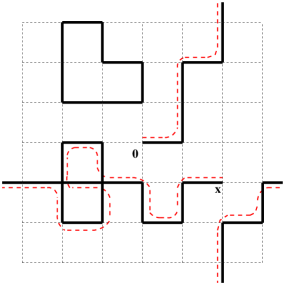
Figure 1: Illustration of an Ising high-temperature graph and its corresponding Ising walk. The underlying graph, $G$, is the discrete two-dimensional torus with $L=7$, with the natural lexicographic order imposed on the vertices. The solid black lines denote a high-temperature edge configuration $A\in\mathcal{C}_{x}$, while the red dashed line denotes $\mathcal{T}(A)$. The walk length is $|\mathcal{T}|=23$.

Partitioning $\Omega_{G}$ in terms of $\mathcal{T}$ we can write, for any $v\in V$,

$$\mathbb{E}(\sigma_{0}\sigma_{v}) =\sum_{\omega\in\Omega_{G}}\sum_{\begin{subarray}{c}A\in\mathcal{C}_{v}\\ \mathcal{T}(A)=\omega\end{subarray}}\frac{[\tanh(\beta)]^{|A|}}{\lambda(\mathcal{C}_{0})}$$ (5)

$$=\sum_{\begin{subarray}{c}\omega\in\Omega_{G}\\ \omega:0\to v\end{subarray}}\rho(\omega)$$ (6)

where $\rho:\Omega_{G}\to[0,\infty)$ is defined by

$$\rho(\omega):=\frac{\lambda(\mathcal{T}^{-1}(\omega))}{\lambda(\mathcal{C}_{0})}.$$ (7)

Note that, by definition [27], the two-point function for SAW on $G$ is again of the form (6), but with the weight given by

$$\rho(\omega)=J^{|\omega|}{\mathds{1}}(\text{$\omega$ is self-avoiding})$$ (8)

where $J\in(0,\infty)$ is a parameter, referred to as the fugacity.

2.2 Unwrapping and winding

Let $\mathbb{T}_{L}^{d}$ denote the $d$-dimensional discrete torus of period $L$. In what follows we identify the vertex set of $\mathbb{T}_{L}^{d}$ with $[-L/2,L/2)^{d}\cap\mathbb{Z}^{d}$. In defining $\Omega_{\mathbb{T}_{L}^{d}}$ and $\Omega_{\mathbb{Z}^{d}}$ we take the root to be the origin.

Let $\mathcal{W}:\Omega_{\mathbb{Z}^{d}}\to\Omega_{\mathbb{T}_{L}^{d}}$ denote the canonical bijection which wraps a $\mathbb{Z}^{d}$-walk onto a $\mathbb{T}_{L}^{d}$-walk. Explicitly, for each $\omega\in\Omega_{\mathbb{Z}^{d}}$, the image $\tau=\mathcal{W}(\omega)$ is defined recursively by setting $\tau_{0}=\omega_{0}=0$, and then for $0\leq i\leq|\omega|-1$ letting

$$\tau_{i+1}=\begin{cases}\tau_{i}+(\omega_{i+1}-\omega_{i}),&\tau_{i}+(\omega_{i+1}-\omega_{i})\in\mathbb{T}_{L}^{d},\\ \tau_{i}+(1-L)(\omega_{i+1}-\omega_{i}),&\tau_{i}+(\omega_{i+1}-\omega_{i})\not\in\mathbb{T}_{L}^{d}.\end{cases}$$ (9)

The number of windings of a $\mathbb{T}_{L}^{d}$-walk along any specified coordinate axis can be conveniently expressed in terms of $\mathcal{W}$. In particular, if $(x)_{i}$ denotes the $i$th coordinate of $x\in\mathbb{Z}^{d}$, the winding number of $\omega\in\Omega_{\mathbb{T}_{L}^{d}}$ along the first coordinate axis is

$$\mathcal{R}(\omega):=\left\lfloor\frac{|(e\circ\mathcal{W}^{-1}(\omega))_{1}|}{L}\right\rfloor.$$ (10)

As an illustration, consider $d=1$, $L=4$, and the walk $\omega=0,-1,-2,1,0,-1,-2,1$, which only takes steps to the left. Then $|\omega|=7$, $e\circ\mathcal{W}^{-1}(\omega)=-7$ and $\mathcal{R}(\omega)=1$.

For given $\rho:\Omega_{\mathbb{T}_{L}^{d}}\to[0,\infty)$ we define the corresponding two-point function $g_{\rho}:\mathbb{T}_{L}^{d}\to[0,\infty)$ via

$$g_{\rho}(x):=\sum_{\tau\in\Omega_{\mathbb{T}_{L}^{d}}}\rho(\tau){\mathds{1}}[e(\tau)=x]$$ (11)

and the corresponding unwrapped two-point function $\tilde{g}_{\rho}:\mathbb{Z}^{d}\to[0,\infty)$ via

$$\tilde{g}_{\rho}(z) :=\sum_{\tau\in\Omega_{\mathbb{T}_{L}^{d}}}\rho(\tau)\,{\mathds{1}}[e(\mathcal{W}^{-1}(\tau))=z]$$ (12)

$$=\sum_{\zeta\in\Omega_{\mathbb{Z}^{d}}}\rho\circ\mathcal{W}(\zeta)\,{\mathds{1}}[e(\zeta)=z].$$ (13)

We emphasise that if the weights are chosen via (7) or (8), then (11) reduces, respectively, to the Ising or SAW two-point functions considered in the previous section, specialised to the torus. Similarly, the unwrapped Ising and SAW two-point functions are defined by (12) specialised to (7) and (8), respectively.

We also note that, following immediately from the definitions, we have

$$g_{\rho}(x)=\sum_{z\in\mathbb{Z}^{d}}\tilde{g}_{\rho}(x+zL).$$ (14)

In this sense, the unwrapped two-point function is therefore a more fine-grained object than the torus two-point function.

2.3 SAW and Ising walk distributions

We now describe in more detail the specific SAW and Ising walk ensembles which we study. We consider the variable-length ensemble of SAWs on $\mathbb{T}_{L}^{d}$, which corresponds to the set of all SAWs on $\mathbb{T}_{L}^{d}$, rooted at the origin, and chosen randomly with a measure proportional to the weight given in (8). Let $\mathcal{S}$ denote a random SAW chosen via this measure. We will be interested in the distribution of the walk length $|\mathcal{S}|$, defined in (4), and winding number $\mathcal{R}(\mathcal{S})$, defined in (10). Moreover, it follows immediately from (12) and (8) that the unwrapped SAW two-point function can be expressed in terms of $\mathcal{S}$ via

$$\tilde{g}_{\rho}(z)=\frac{\mathbb{P}[e(\mathcal{W}^{-1}\circ\mathcal{S})=z]}{\mathbb{P}[|\mathcal{S}|=0]},\qquad z\in\mathbb{Z}^{d}.$$ (15)

Our simulations of $\mathcal{S}$, discussed below, were performed using a lifted version [28] of the Berretti-Sokal algorithm [29].

Now let us consider the Ising walk $\mathcal{T}$. To begin, consider the probability measure on the state space $\cup_{x\in\mathbb{T}_{L}^{d}}\mathcal{C}_{x}$, such that the probability of $A\in\cup_{x\in\mathbb{T}_{L}^{d}}\mathcal{C}_{x}$ is proportional to $[\tanh(\beta)]^{|A|}$. Let $\mathcal{A}$ denote a random sample drawn from this measure. The distribution of $\mathcal{A}$ is precisely the stationary distribution of the Prokofiev-Svistunov worm algorithm [30], in which the worm tail is fixed to the origin. Our simulations of $\mathcal{A}$, discussed below, were performed using such a worm algorithm. We will be interested in the induced distribution of $\mathcal{T}(\mathcal{A})$. For simplicity, we will henceforth adopt the abbreviation $\mathcal{T}=\mathcal{T}(\mathcal{A})$.

Analogously to SAW, it follows from (12) and (7) that the unwrapped Ising two-point function can be expressed exactly as in (15), with $\mathcal{S}$ replaced by $\mathcal{T}$. Also analogously to SAW, we will again consider the induced distributions of $|\mathcal{T}|$ and $\mathcal{R}(\mathcal{T})$, which we refer to as the Ising walk length and Ising winding number.

2.4 Random-length random walks

Let $(C_{n})_{n\in\mathbb{N}}$ be an i.i.d. sequence of uniformly random elements of $\{\pm e_{1},...,\pm e_{d}\}$, where $e_{i}=(0,\ldots,1,\ldots,0)\in\mathbb{Z}^{d}$ is the standard unit vector along the $i$th coordinate axis. Let $S_{0}=0$ and for $n\geq 0$ set $S_{n+1}=S_{n}+C_{n+1}$. Now let $\mathcal{N}$ be an $\mathbb{N}$-valued random variable independent of $(C_{n})_{n\in\mathbb{N}}$. The corresponding Random-length Random Walk on $\mathbb{Z}^{d}$ is the process $\mathcal{Z}:=(S_{n})_{n=0}^{\mathcal{N}}$. Similarly, $\mathcal{X}:=\mathcal{W}(\mathcal{Z})$ is the corresponding RLRW on $\mathbb{T}_{L}^{d}$, where $\mathcal{W}$ is the wrapping bijection defined in (9).

We also consider a loop-erased version of RLRW, constructed as follows. Recursively define a simple random walk $(R_{i})_{i\in\mathbb{N}}$ on $\mathbb{T}_{L}^{d}$ by applying (9) to $(S_{i})_{i\in\mathbb{N}}$, and then perform chronological loop erasure on $(R_{i})_{i\in\mathbb{N}}$ until a walk of length $\mathcal{N}$ is generated. We refer to the resulting walk, denoted $\mathcal{L}$, as the random-length loop-erased random walk (RLLERW) on $\mathbb{T}_{L}^{d}$. Note that $\mathcal{N}$ must be bounded above by $L^{d}$ in order for $\mathcal{L}$ to be well defined.

We define the two-point function of $\mathcal{Z}$ to be

$$\mathbb{E}\Bigg{(}\sum_{n=0}^{|\mathcal{Z}|}{\mathds{1}}(\mathcal{Z}_{n}=x)\Bigg{)}$$ (16)

which gives the expected number of visits of $\mathcal{Z}$ to $x\in\mathbb{Z}^{d}$. Analogous definitions hold for the RLRW and RLLERW on $\mathbb{T}_{L}^{d}$ by replacing $\mathcal{Z}$ with $\mathcal{X}$ and $\mathcal{L}$, respectively. As noted in the Introduction, in the special case in which $\mathcal{N}$ is geometrically distributed, the two-point function of RLRW on $\mathbb{Z}^{d}$ corresponds to the lattice Green function, which is very well studied; see [18] and references therein.

A simple rearrangement of (16) (see A) shows that it can be expressed in the form (6) with

$$\rho(\omega)=\frac{\mathbb{P}(\mathcal{N}\geq|\omega|)}{(2d)^{|\omega|}},\qquad\omega\in\Omega_{\mathbb{Z}^{d}}.$$ (17)

Precisely the same statement also holds for $\mathcal{X}$, with the same weights, but replacing $\Omega_{\mathbb{Z}^{d}}$ with $\Omega_{\mathbb{T}_{L}^{d}}$. Moreover, an analogous statement also holds for $\mathcal{L}$ with (see A)

$$\rho(\omega)=\mathbb{P}(\mathcal{L}\sqsupseteq\omega),$$ (18)

where for any two walks $\tau,\omega\in\Omega_{\mathbb{T}_{L}^{d}}$, the notation $\tau\sqsupseteq\omega$ implies that $|\tau|\geq|\omega|$ and $\tau_{i}=\omega_{i}$ for all $0\leq i\leq|\omega|$.

The unwrapped two-point functions of $\mathcal{Z}$, $\mathcal{X}$, and $\mathcal{L}$ are defined by (12), with the appropriate choices of weight $\rho$ just outlined. Now, since for any $\omega\in\Omega_{\mathbb{Z}^{d}}$ we have $|\mathcal{W}(\omega)|=|\omega|$, it follows from (13) and (17) that the unwrapped two-point function of $\mathcal{X}$ is simply

$$\tilde{g}_{\rho}(z) =\sum_{\zeta\in\Omega_{\mathbb{Z}^{d}}}\mathbb{P}(\mathcal{N}\geq|\zeta|)\frac{{\mathds{1}}(e(\zeta)=z)}{(2d)^{|\zeta|}}$$

$$=\sum_{n=0}^{\infty}\mathbb{P}(\mathcal{N}\geq n)\sum_{\zeta\in\Omega_{\mathbb{Z}^{d}}^{n}}\frac{{\mathds{1}}(e(\zeta)=z)}{(2d)^{|\zeta|}}$$

$$=\sum_{n=0}^{\infty}\mathbb{P}(\mathcal{N}\geq n)\mathbb{P}(S_{n}=z)$$

$$=\mathbb{E}\left(\sum_{n=0}^{|\mathcal{Z}|}{\mathds{1}}(\mathcal{Z}_{n}=z)\right).$$ (19)

In other words, the unwrapped two-point function of the RLRW on the torus is simply the two-point function of the corresponding RLRW on $\mathbb{Z}^{d}$. Now, for an appropriate choice of distribution for $\mathcal{N}$, the unwrapped two-point function of $\mathcal{X}$ is expected to display the same asymptotics as the unwrapped two-point functions for the SAW and Ising walk. This then motivates studying the two-point function of $\mathcal{Z}$, which we do in Sections 3.3 and 4.

Finally, we note that, after some rearrangement (see A), the unwrapped two-point function of $\mathcal{L}$ can be expressed as

$$\tilde{g}_{\rho}(z)=\mathbb{P}[\mathcal{W}^{-1}(\mathcal{L})\ni z],$$ (20)

which can be easily estimated via simulation.

2.5 Numerical details

Our simulations of the Ising model were performed at the exact infinite-volume critical point in two dimensions [31], and at the estimated location of the infinite-volume critical point $\tanh(\beta_{\mathrm{c}})=0.113~{}424~{}8(5)$ [2] in five dimensions. The SAW model was simulated at the estimated location of the infinite-volume critical points, $J_{\mathrm{c}}=0.379~{}052~{}277~{}758(4)$ [32] in two dimensions, $J_{\mathrm{c}}=0.113~{}140~{}84(1)$ [28] in five dimensions, and $J_{\mathrm{c}}=0.091~{}927~{}86(4)$ [33] in six dimensions.

For the Ising model, we simulated linear system sizes up to $L=31$ in five dimensions. For SAW, we simulated linear system sizes up to $L=221$ in five dimensions, and $L=57$ in six dimensions. For the RLLERW, we simulated linear system sizes up to $L=161$ in five dimensions.

Our error estimation follows standard procedures, see for instance [34, 35]. Analyses of integrated autocorrelation times for the worm and irreversible Berretti-Sokal algorithms are presented in [36] and [28], respectively.

3 Results

3.1 Universal walk length distribution

Let $\mathcal{K}$ denote a self-avoiding walk on the complete graph $K_{n}$, rooted at a fixed vertex, distributed according to the variable-length ensemble. The probability distribution of $\mathcal{K}$ is then proportional to the weight given in (8). It was shown in [19] that the critical fugacity for $\mathcal{K}$ occurs at $J=1/n$. Furthermore, at criticality, it is known [22, Theorem 1.1] (see also [19, 23]) that

$$\begin{split}\mathbb{E}(|\mathcal{K}|)&\sim\sqrt{\frac{2}{\pi}}\sqrt{n}\\ \mathrm{var}(|\mathcal{K}|)&\sim\left(1-\frac{2}{\pi}\right)n.\end{split}$$ (21)

From universality, one would then expect that if one considered the walk lengths of the critical SAW or Ising models on $\mathbb{T}_{L}^{d}$ with $d>d_{\rm c}$, then their means should scale as $L^{d/2}$, and their variances should scale as $L^{d}$. Figure 2 provides strong evidence that this is the case.

As a simple consequence, this would imply that the ratio of the mean and standard deviation of the walk length therefore converges to a positive constant. From (21), the value of this constant for $\mathcal{K}$ is

$$\lim_{n\to\infty}\frac{\mathbb{E}(|\mathcal{K}|)}{\sqrt{\mathrm{var}(|\mathcal{K}|)}}=\sqrt{\frac{2}{\pi-2}}=:\varphi$$ (22)

For comparison, the analogous ratio for the SAW and Ising models on $\mathbb{T}_{L}^{d}$ is plotted in Figure 3(a). The SAW data suggest it is plausible, for both $d=5$ and $d=6$, that $\mathbb{E}(|\mathcal{S}|)/\sqrt{\mathrm{var}(|\mathcal{S}|)}$ is converging to the complete graph value, $\varphi$. The $d=5$ Ising data suggest, however, that $\mathbb{E}(|\mathcal{T}|)/\sqrt{\mathrm{var}(|\mathcal{T}|)}$ is converging to a constant strictly less than $\varphi$, although it is certainly numerically close to $\varphi$.

In addition to the asymptotic moments given in (21), central limit theorems have been established for $\mathcal{K}$. Indeed, it follows from [22, Theorem 1.2] (see also [23, Theorem 1.3]) that, at criticality,

$$\lim_{n\to\infty}\mathbb{P}\left(\frac{|\mathcal{K}|-\mathbb{E}(|\mathcal{K}|)}{\sqrt{\mathrm{var}(|\mathcal{K}|)}}\leq x\right)=\mathbb{P}\left(\frac{|X|-\mathbb{E}(|X|)}{\sqrt{\mathrm{var}(|X|)}}\leq x\right)$$ (23)

for all $x\in\mathbb{R}$, where $X$ is a standard normal random variable. We note that the law of $|X|$ is the half-normal distribution, which can be given explicitly by

$$\mathbb{P}(|X|\leq x)={\mathds{1}}(x>0)[1-2\bar{\Phi}(x)]$$ (24)

where $\bar{\Phi}$ denotes the standard normal tail distribution, so that for all $x\in\mathbb{R}$

$$\bar{\Phi}(x):=\frac{1}{\sqrt{2\pi}}\int_{x}^{\infty}\rme^{-s^{2}/2}{\rm d}s.$$ (25)

For later reference, we shall denote by $F$ the law of the standardised version of $|X|$ appearing on the right-hand side of (23), i.e. for $x\in\mathbb{R}$

$$F(x):=\mathbb{P}\left(\frac{|X|-\mathbb{E}(|X|)}{\sqrt{\mathrm{var}(|X|)}}\leq x\right).$$ (26)

By universality, one would expect that the standardised distribution functions of $|\mathcal{S}|$ and $|\mathcal{T}|$ on $\mathbb{T}_{L}^{d}$ should also converge to $F$. Figure 3 (right panel) provides strong evidence that this is indeed the case.

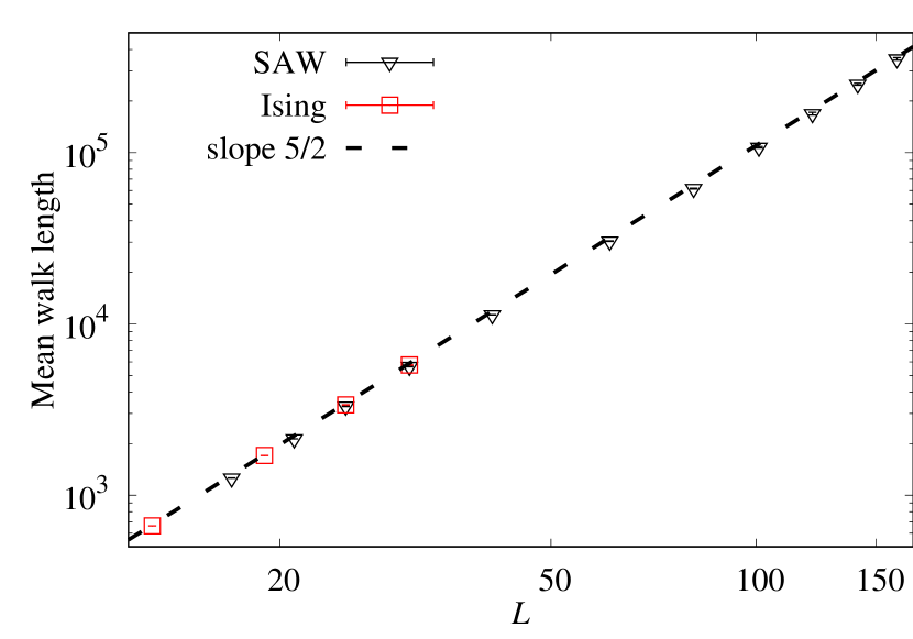
(a)

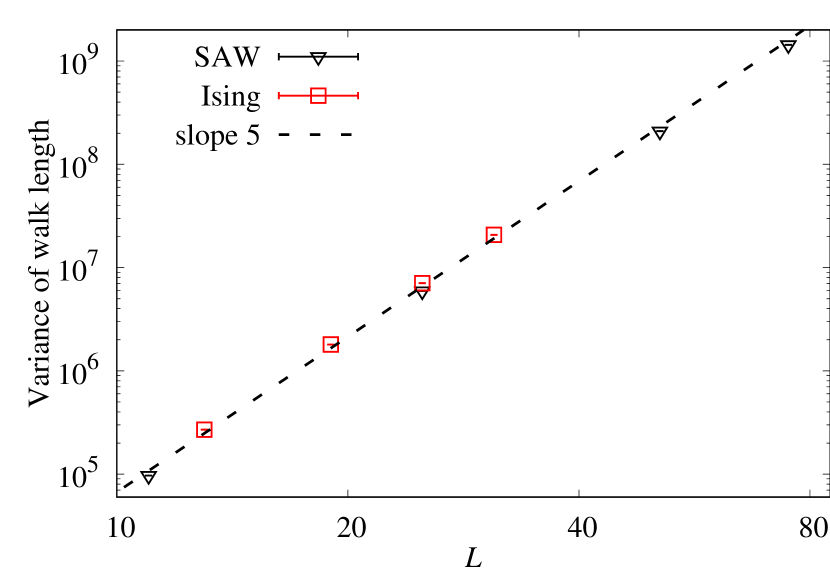
(b)

Figure 2: (2(a)) Simulated mean of the critical SAW and Ising walk lengths on five-dimensional tori. (2(b)) Simulated variance of the critical SAW and Ising walk lengths on five-dimensional tori.

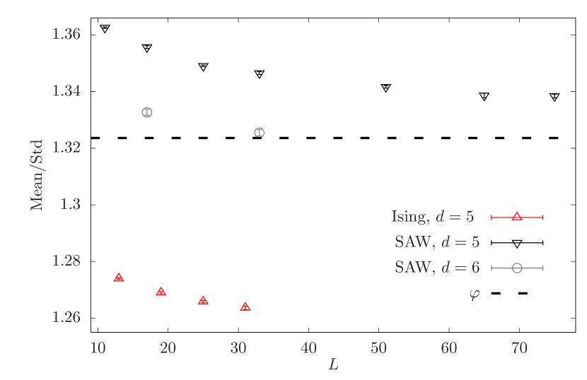
(a)

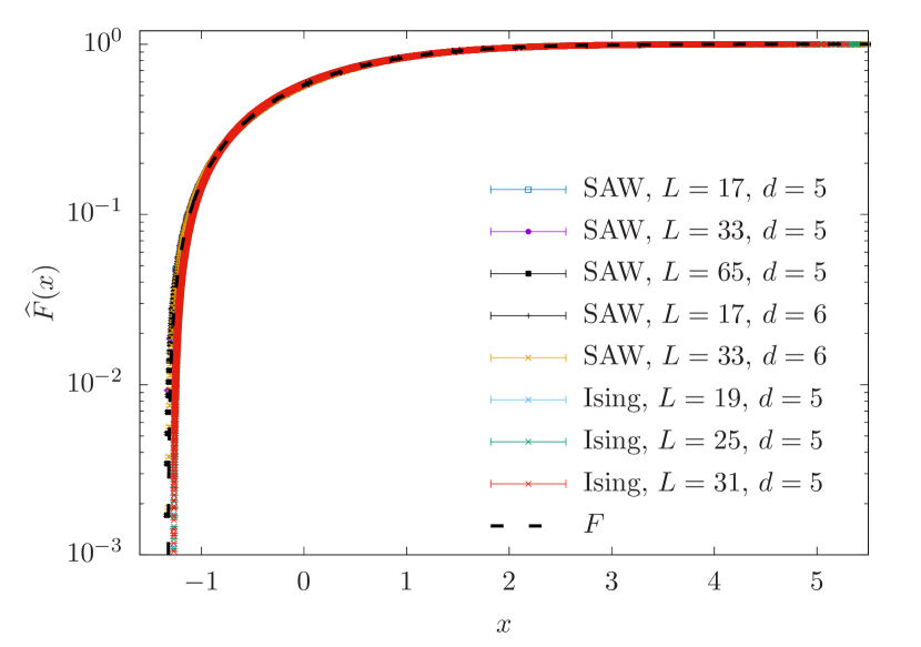
(b)

Figure 3: (3(a)) Ratio of simulated mean and standard deviation of the critical SAW walk length on five- and six-dimensional tori, and the critical Ising walk length on five-dimensional tori. The dashed curve corresponds to the limiting value $\varphi$ for the case of SAW on $K_{n}$; see (22). (3(b)) Simulated distribution function, $\widehat{F}$, of the standardised walk length $(|\mathcal{S}|-\mathbb{E}(|\mathcal{S}|))/\sqrt{\mathrm{var}(|\mathcal{S}|)}$ for critical SAW on five- and six-dimensional tori, as well as the standardised critical Ising walk length $(|\mathcal{T}|-\mathbb{E}(|\mathcal{T}|))/\sqrt{\mathrm{var}(|\mathcal{T}|)}$ on five-dimensional tori. The dashed curve corresponds to $F$ given in (26).

3.2 Proliferation of windings

We now consider the large $L$ asymptotics of $\mathbb{E}(\mathcal{R})$. Fig. 4 plots $\mathbb{E}(\mathcal{R})$ with $d=2,5,6$ for SAW, and $d=2,5$ for the Ising model. In dimensions below $d_{\rm c}$, we find that $\mathbb{E}(\mathcal{R})$ is bounded as $L\to\infty$. By contrast, we observe that windings proliferate for $d>d_{\rm c}$. It was conjectured in [6] that $\mathbb{E}(\mathcal{R})$ should scale as $L^{d/4-1}$ at criticality when $d>d_{\rm c}$. For $d=5$, fitting $\mathbb{E}(\mathcal{R})$ to a power law ansatz produces an exponent value of $0.24(3)$ for the Ising model and $0.30(6)$ for SAW. For $d=6$ SAW, the analogous fit yields an exponent value of $0.46(6)$. In each case, the estimated and conjectured exponent values agree within error bars. We note that, in the Ising case, the definition of $\mathcal{R}$ considered here differs from that used in [6], the current version be a more natural analogue of the SAW definition. The asymptotic behaviour is the same in both cases however.

Finally, we also studied the average winding number of a RLLERW with $d=5$ whose walk length is drawn from the asymptotic walk length distribution of the complete-graph SAW; i.e. with standardised distribution function $F$, and with mean and variance given by the right-hand side of (21) with $n=L^{d}$. Our fits lead to the exponent value $0.29(5)$, in agreement with the SAW and Ising models.

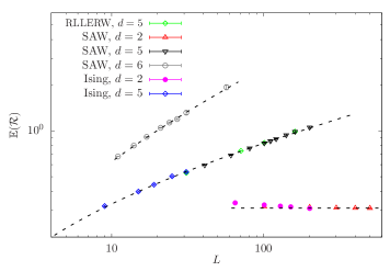
Figure 4: Simulated values of $\mathbb{E}(\mathcal{R})$ for the critical Ising and SAW models, on discrete tori in various dimensions. Analogous results are also shown for RLLERW with $d=5$ and walk length chosen via the asymptotic distribution of SAW on the complete-graph. To emphasise the universal scaling, the data for all models in each given dimension were translated onto a single curve by multiplying by suitable ($L$-independent) constants. The number of windings is clearly asymptotically constant in $L$ for $d<d_{\rm c}$, while above $d_{\rm c}$ windings proliferate as $L$ increases.

3.3 Unwrapped two-point functions

We begin by stating the following proposition for the two-point function of RLRW on $\mathbb{Z}^{d}$. The proof is deferred to Section 4. We emphasise that, due to (19), Proposition 3.1 also immediately implies the analogous result for the unwrapped two-point function of RLRW on the torus.

Proposition 3.1.

Consider a sequence of $\mathbb{N}$-valued random variables $\mathcal{N}_{L}$, such that there exists a non-decreasing sequence $a_{L}>0$ for which $\mathcal{N}_{L}/a_{L}$ converges in distribution, as $L\to\infty$, to a random variable with distribution function $G$. Now fix an integer $d\geq 3$, and let $z_{L}\in\mathbb{Z}^{d}$ be a sequence such that $\|z_{L}\|\to\infty$ as $L\to\infty$, with $\xi:=\lim_{L\to\infty}\|z_{L}\|/\sqrt{a_{L}}\in(0,+\infty]$ well defined . Then, the two-point function of $\mathcal{Z}$ satisfies

$$\lim_{L\rightarrow\infty}\|z_{L}\|^{d-2}g(z_{L})=\frac{d}{2\pi^{d/2}}\int_{0}^{\infty}s^{d/2-2}\rme^{-s}\,\left[1-G\left(\frac{d}{2}\frac{\xi^{2}}{s}\right)\right]{\rm d}s$$

As a first observation, we note that, provided $G$ is continuous at the origin, as $\xi\to 0$ the right-hand side of the limit appearing in Proposition  3.1 reduces to

$$\lim_{\xi\to 0}\frac{d}{2\pi^{d/2}}\int_{0}^{\infty}s^{d/2-2}\rme^{-s}\,\left[1-G\left(\frac{d}{2}\frac{\xi^{2}}{s}\right)\right]{\rm d}s=\frac{d}{2\pi^{d/2}}\Gamma(d/2-1)$$ (27)

in agreement with the well-known asymptotics of the two-point function of simple random walk (see e.g. [17, Theorem 4.3.1]). This is to be expected, since typical walks of length $a_{L}$ explore a ball whose radius is of order $\sqrt{a_{L}}$, and $\xi\to 0$ corresponds to the case where $\sqrt{a_{L}}$ dominates the spatial scale $\|z_{L}\|$ probed, meaning the walk length grows so fast that the finiteness of the walk is not observed.

We are particularly interested in the case where $G$ corresponds to the SAW and Ising models on high-dimensional tori. The numerical results of Section 3.1 lead to the conjecture that for $d>4$ at criticality $\mathbb{E}(|\mathcal{S}|)\sim B_{\mathcal{S},d}L^{d/2}$ and $\sqrt{\mathrm{var}(|\mathcal{S}|)}\sim A_{\mathcal{S},d}L^{d/2}$, and $(|\mathcal{S}|-\mathbb{E}(|\mathcal{S}|))/\sqrt{\mathrm{var}(|\mathcal{S}|)}$ converges weakly to $F$, where $A_{\mathcal{S},d},B_{\mathcal{S},d}>0$ and $F$ is as given in (26). Assuming the validity of this conjecture, it follows from standard convergence of types arguments (see e.g. [37, pp. 193]) that

$$\lim_{L\to\infty}\mathbb{P}\left(\frac{\mathcal{S}}{L^{d/2}}\leq x\right)=F\left(\frac{x-B_{\mathcal{S},d}}{A_{\mathcal{S},d}}\right)$$ (28)

for all $x\in\mathbb{R}$.

Now let $\mathcal{N}=|\mathcal{S}|$, $a_{L}=L^{d/2}$ and for fixed $\xi\in(0,\infty)$ let $z_{L}=\lfloor L^{d/4}\xi\rfloor e_{1}$. Assuming the validity of (28) it follows from Proposition 3.1 that as $L\to\infty$ the unwrapped two-point function of the corresponding RLRW on $\mathbb{T}_{L}^{d}$ satisfies

$$\|z_{L}\|^{d-2}\,\tilde{g}(z_{L})\sim H_{d}(1,1/A_{\mathcal{S},d},B_{\mathcal{S},d}/A_{\mathcal{S},d};\xi)$$ (29)

where

$$H_{d}(\alpha,\beta,\gamma;\xi):=\alpha\frac{d}{2\pi^{d/2}}\,\int_{0}^{\infty}s^{d/2-2}e^{-s}\left[1-F\left(\beta\,\frac{d\xi^{2}}{2s}-\gamma\right)\right]{\rm d}s.$$ (30)

Universality then makes it natural to conjecture that the asymptotics of $\|z_{L}\|^{d-2}\,\tilde{g}(z_{L})$ for the SAW and Ising models on the torus should also be given by $H_{d}(\alpha,\beta,\gamma;\xi)$, for suitable model-dependent values of the constants, $\alpha,\beta,\gamma$. Figures 5(b) and 5(c) provide strong evidence in favour of these conjectures. In Figure 5(b), the constants for SAW are set to $\alpha=0.85$, $\beta=1.5/A_{\mathcal{S},d}$, and $\gamma=B_{\mathcal{S},d}/A_{\mathcal{S},d}$, while in 5(c) the constants for the Ising model are set to $\alpha=1$, $\beta=1.2/A_{\mathcal{T},d}$ and $\gamma=B_{\mathcal{T},d}/A_{\mathcal{T},d}$.

In addition to the Ising and SAW cases, in Figure 5(d) we plot the two-point function for RLLERW with walk length chosen via the asymptotic distribution of SAW on the complete-graph, which again appears to be described by $H_{d}(\alpha,\beta,\gamma;\xi)$. In this case, we set $\alpha=0.75$, $\beta=1.2/\sqrt{1-2/\pi}$ and $\gamma=\varphi$; c.f. (21) and (22).

We note that the two-point functions of the critical SAW [16, Theorem 1.1] and Ising [15, Theorem 1.3] models on $\mathbb{Z}^{d}$ are known to satisfy

$$\lim_{\|z\|\to\infty}\|z\|^{d-2}\,g(z)=A\frac{d}{2\pi^{d/2}}\Gamma(d/2-1)$$ (31)

where the non-universal constant $A$ can be expressed in terms of quantities appearing in the lace expansion. Our conjecture, if true, would therefore provide natural finite-size analogues/refinements of [16, Theorem 1.1] and [15, Theorem 1.3]. We remark that for SAW in $d=5$ it follows rigorously from bounds established in [38] that $0.81<A<0.92$; the value of $\alpha=0.85$ used in Figure 5(b) for $d=5$ SAW is therefore consistent with these rigorous bounds on the value of $A$.

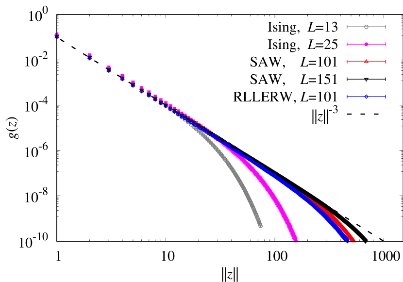
(a)

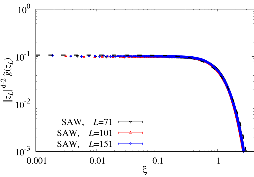
(b)

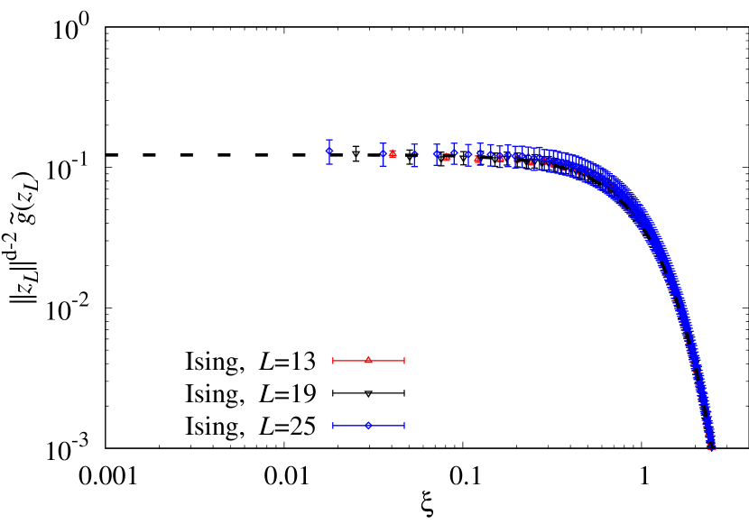
(c)

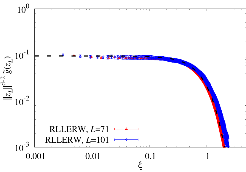
(d)

Figure 5: (5(a)) Unwrapped two-point functions on the five-dimensional torus, of the critical Ising and SAW models, and RLLERW whose walk length is drawn from the asymptotic walk length distribution of the complete-graph SAW. Standard SRW behaviour is clearly displayed in the bulk of the system. (5(b)) Plot of $\|z_{L}\|^{d-2}\tilde{g}(z_{L})$ vs $\xi$ for SAW on five-dimensional tori. The dashed curve shows $H(\alpha,\beta,\gamma;\xi)$ with constants $\alpha,\beta,\gamma$ set to the values described in the text, with $A_{\mathcal{S},d}$ and $B_{\mathcal{S},d}$ estimated via simulation. (5(c)) Analogous plot to (5(b)), for the Ising case. (5(d)) Analogous plot to (5(b)), for case of RLLERW whose walk length is drawn from the asymptotic walk length distribution of the complete-graph SAW.

4 Proof of Proposition 3.1

Let $(S_{n})_{n=0}^{\infty}$ be a simple random walk on $\mathbb{Z}^{d}$, starting from the origin, and let

$$p_{n}(z):=\mathbb{P}(S_{n}=z),\qquad z\in\mathbb{Z}^{d}.$$ (32)

We say that $n\in\mathbb{N}$ and $z\in\mathbb{Z}^{d}$ have the same parity, and write $n\leftrightarrow z$, iff $n+\|z\|_{1}$ is even. Clearly, $p_{n}(z)=0$ if $n\nleftrightarrow z$. The main tool used to prove Proposition 3.1 is the local central limit theorem for $(S_{n})_{n=0}^{\infty}$, which allows $p_{n}(z)$ to be approximated, when $n$ is large, by

$$\bar{p}_{n}(z):=2\left(\frac{d}{2\pi n}\right)^{d/2}\exp\left(-\frac{d\|z\|^{2}}{2n}\right),\qquad z\in\mathbb{Z}^{d},\,n\geq 1.$$ (33)

In particular, we will apply the following lemma, whose proof we defer until the end of this section.

Lemma 4.1.

Fix a positive integer $d$, and let $z_{L}\in\mathbb{Z}^{d}$ be a sequence for which $\|z_{L}\|\to\infty$ as $L\to\infty$. Then for any $\epsilon>0$, as $L\to\infty$

1. $\sum\limits_{n=1}^{\infty}|p_{n}(z_{L})-\bar{p}_{n}(z_{L})|=O(\|z_{L}\|^{-d+\epsilon})$

2. $\sum\limits_{n=1}^{\infty}|\bar{p}_{n}(z_{L})-\bar{p}_{n+1}(z_{L})|=O(\|z_{L}\|^{-d+\epsilon})$

Proof of Proposition 3.1.

Let $\mathcal{N}$ be an $\mathbb{N}$-valued random variable, independent of $(S_{n})_{n=0}^{\infty}$. It follows from the definition (16) that for all $z\in\mathbb{Z}^{d}$

$$g(z)=\mathbb{E}\,\sum_{n=0}^{\infty}{\mathds{1}}(\mathcal{N}\geq n){\mathds{1}}(S_{n}=z)=\sum_{n=0}^{\infty}\,\mathbb{P}(\mathcal{N}\geq n)\,p_{n}(z).$$

Moreover, if $z\neq 0$ we have

$$g(z) =\sum_{n=1}^{\infty}\,\mathbb{P}(\mathcal{N}\geq n)\,p_{n}(z)\,{\mathds{1}}(z\leftrightarrow n)$$

$$=D(z)+E_{1}(z)+E_{2}(z)$$

where

$$D(z) :=\sum_{n=1}^{\infty}\frac{\bar{p}_{n}(z)}{2}\,\mathbb{P}(\mathcal{N}\geq n),$$ (34)

$$E_{1}(z) :=\sum_{n=1}^{\infty}\frac{\bar{p}_{n}(z)}{2}\,\mathbb{P}(\mathcal{N}\geq n){\mathds{1}}(z\leftrightarrow n)-\sum_{n=1}^{\infty}\frac{\bar{p}_{n}(z)}{2}\,\mathbb{P}(\mathcal{N}\geq n){\mathds{1}}(z\not\leftrightarrow n),$$ (35)

$$E_{2}(z) =\sum_{n=1}^{\infty}\,\mathbb{P}(\mathcal{N}\geq n)\,\left[p_{n}(z)-\bar{p}_{n}(z)\right]\,{\mathds{1}}(z\leftrightarrow n).$$ (36)

We consider each of these three terms in turn, beginning with $D$. If $a:(0,\infty)\to(0,\infty)$ is non-increasing and $b:(0,\infty)\to(0,\infty)$ is non-decreasing, then for any positive integer $k$ one has

$$\int_{k-1}^{\infty}a(t+1)b(t){\rm d}t\leq\sum_{n=k}^{\infty}a(n)b(n)\leq\int_{k}^{\infty}a(t-1)b(t){\rm d}t.$$ (37)

Applying (37) with $a(n)=n^{-d/2}\,\mathbb{P}(\mathcal{N}>n-1)$ and $b(n)=e^{-d\|z\|^{2}/2n}$, and changing integration variables, yields

$$\int_{0}^{\infty}s^{d/2-2}e^{-s}\left(1+\frac{2s}{d\|z\|^{2}}\right)^{-d/2}\mathbb{P}\left(\frac{2\mathcal{N}}{d\|z\|^{2}}>s^{-1}\right){\rm d}s\\ \leq\frac{2\pi^{d/2}}{d}\|z\|^{d-2}D(z)\leq\\ \frac{\pi^{d/2}}{d}\|z\|^{d-2}\bar{p}_{1}(z)+\int_{0}^{d\|z\|^{2}/4}s^{d/2-2}e^{-s}\left(1-\frac{2s}{d\|z\|^{2}}\right)^{-d/2}\mathbb{P}\left(\frac{2\mathcal{N}}{d\|z\|^{2}}>s^{-1}-\frac{4}{d\|z\|^{2}}\right){\rm d}s$$ (38)

In the upper bound, the $\bar{p}_{1}(z)$ term is treated separately since $a(t-1)b(t)$ is not integrable on $(1,\infty)$.

Now consider sequences $\mathcal{N}_{L}$, $a_{L}$ and $z_{L}$ as described in the statement of the proposition, and substitute $\mathcal{N}=\mathcal{N}_{L}$ and $z=z_{L}$ in (38). Since $a_{L}$ is positive and non-decreasing, it either converges to a strictly positive limit, or diverges to $+\infty$. Consequently, since $\mathbb{P}(\mathcal{N}_{L}/a_{L}\leq\cdot)$ converges weakly to $G$ as $L\to\infty$, standard convergence of types arguments (see e.g. [37, pp. 193]), imply that, for any fixed $c\in\mathbb{R}$ and almost every $y\in\mathbb{R}$, as $L\to\infty$ we have

$$\lim_{L\to\infty}\mathbb{P}\left(\frac{\mathcal{N}_{L}}{a_{L}}\leq\frac{d\|z_{L}\|^{2}}{2a_{L}}\,y-\frac{c}{a_{L}}\right)=G\left(\frac{d}{2}\,\xi^{2}\,y\right).$$ (39)

Then, since $s^{d/2-2}e^{-s}$ is integrable on $(0,\infty)$ when $d\geq 3$, applying Lebesgue’s dominated convergence theorem to the integrals in the lower and upper bounds in (38) shows, in both cases, that the limits as $L\to\infty$ exist and equal

$$\int_{0}^{\infty}s^{d/2-2}e^{-s}[1-G(d\xi^{2}/2s)]{\rm d}s.$$

It then follows from (38) that

$$\lim_{L\to\infty}\|z_{L}\|^{d-2}D(z_{L})=\frac{d}{2\pi^{d/2}}\int_{0}^{\infty}s^{d/2-2}e^{-s}[1-G(d\xi^{2}/2s)]{\rm d}s.$$ (40)

We now consider $E_{1}$. Let $z\in\mathbb{Z}^{d}$ and $n\in\mathbb{Z}_{+}$. Since ${\mathds{1}}(z\not\leftrightarrow n)={\mathds{1}}(z\leftrightarrow n+1)$, changing variables via $n\mapsto n+1$ in the first sum in (35) yields

$$2E_{1}(z)\leq\bar{p}_{1}(z)+\sum_{n=1}^{\infty}\left|\bar{p}_{n+1}(z)-\bar{p}_{n}(z)\right|,$$

while changing variables the second sum yields

$$2E_{1}(z)\geq-\left(\bar{p}_{1}(z)+\sum_{n=1}^{\infty}\left|\bar{p}_{n+1}(z)-\bar{p}_{n}(z)\right|\right).$$

It then follows from Lemma 4.1 that $E_{1}(z_{L})=O(\|z_{L}\|^{-d+\epsilon})$ as $L\to\infty$, for every $\epsilon>0$, and so

$$\lim_{L\to\infty}\|z_{L}\|^{d-2}\,E_{1}(z_{L})=0.$$ (41)

Finally, now consider $E_{2}$. In this case, Lemma 4.1 immediately implies that $E_{2}(z_{L})=O(\|z_{L}\|^{-d+\epsilon})$ as $L\to\infty$, for every $\epsilon>0$, and so

$$\lim_{L\to\infty}\|z_{L}\|^{d-2}\,E_{2}(z_{L})=0.$$ (42)

The stated result follows by combining (40), (41) and (42). ∎

We now turn to the proof of Lemma 4.1.

Proof of Lemma 4.1.

The local central limit theorem for random walk (see e.g.[39, Theorem 1.2.1]) implies that there exists $c_{1}\in(0,\infty)$ such that for all $n\in\mathbb{Z}_{+}$ and $z\in\mathbb{Z}^{d}$ we have

$$|\bar{p}_{n}(z)-p_{n}(z)|\leq c_{1}n^{-d/2-1}.$$ (43)

Similarly, it can be shown (see e.g.[40, Lemma 6.1]) that there exists $c_{2}\in(0,\infty)$ such that for all $n\in\mathbb{Z}_{+}$ and $z\in\mathbb{Z}^{d}$ we have

$$|\bar{p}_{n}(z)-\bar{p}_{n+1}(z)|\leq c_{2}n^{-d/2-1}.$$ (44)

Let $a\in\mathbb{Z}_{+}$. It follows from (43), via (37), that

$$\sum_{n=a+1}^{\infty}|\bar{p}_{n}(z)-p_{n}(z)|\leq c_{1}\int_{a+1}^{\infty}(t-1)^{-d/2-1}{\rm d}t=\frac{2}{d}c_{1}a^{-d/2}.$$ (45)

Similarly, it follows from (44) that

$$\sum_{n=a+1}^{\infty}|\bar{p}_{n}(z)-\bar{p}_{n+1}(z)|\leq\frac{2}{d}c_{2}a^{-d/2}.$$ (46)

Now suppose $1\leq n\leq a$. From (33) there exists $c_{3}\in(0,\infty)$ such that

$$\bar{p}_{n}(z),\bar{p}_{n+1}(z)\leq c_{3}\exp\left(-\dfrac{d\|z\|^{2}}{2(a+1)}\right)$$ (47)

But, as shown e.g. in [17, Proposition 2.1.2], there exist $\beta,c_{4}\in(0,\infty)$ such that for all $n\in\mathbb{N}$ and $s>0$

$$\mathbb{P}\left(\max_{0\leq j\leq n}\|S_{j}\|\geq s\sqrt{n}\right)\leq c_{4}e^{-\beta s^{2}}.$$

It then follows that for all $1\leq n\leq a$ and $z\in\mathbb{Z}^{d}$ we have

$$p_{n}(z)\leq c_{4}\exp\left(-\frac{\beta\|z\|^{2}}{a+1}\right).$$ (48)

From (47) and (48) we then conclude that there exist $c_{5},\gamma\in(0,\infty)$, independent of $a$, such that for any $a\in\mathbb{Z}_{+}$ we have

$$\sum_{n=1}^{a}|\bar{p}_{n}(z)-\bar{p}_{n+1}(z)|,\quad\sum_{n=1}^{a}|\bar{p}_{n}(z)-p_{n}(z)|\leq c_{5}\,a\,\exp\left(-\gamma\frac{\|z\|^{2}}{(a+1)}\right).$$ (49)

Now fix $\epsilon\in(0,\infty)$ and let $z\neq 0$. Choosing $a=\lceil\|z\|\rceil^{2-\frac{2\epsilon}{d}}$ implies that the sums in  (49) are exponentially small, and combining with (45) and (46) then implies that for any $\epsilon\in(0,\infty)$ there exists $c\in(0,\infty)$ such that

$$\sum_{n=1}^{\infty}|\bar{p}_{n}(z)-\bar{p}_{n+1}(z)|,\quad\sum_{n=1}^{\infty}|\bar{p}_{n}(z)-\bar{p}_{n+1}(z)|\leq c\|z\|^{-d+\epsilon}.$$ (50)

Both parts of the stated result now follow by specialising to the case $z=z_{L}$. ∎

Appendix A Appendix

A.1 Random-length Random Walk and Random-length LERW

In this brief appendix we provide some details outlining how (17), (18) and (20) can be obtained.

We begin by considering RLRW on $\mathbb{Z}^{d}$. Therefore, let $\rho$ be given by (17) and, let $z\in\mathbb{Z}^{d}$. Then

$$\mathbb{E}\sum_{n=0}^{|\mathcal{Z}|}{\mathds{1}}(\mathcal{Z}_{n}=z) =\mathbb{E}\sum_{n=0}^{\infty}{\mathds{1}}(|\mathcal{Z}|\geq n){\mathds{1}}(\mathcal{Z}_{n}=z)$$

$$=\mathbb{E}\sum_{n=0}^{\infty}{\mathds{1}}(|\mathcal{N}|\geq n){\mathds{1}}(S_{n}=z)$$

$$=\sum_{n=0}^{\infty}\mathbb{P}(|\mathcal{N}|\geq n)\,\mathbb{P}(S_{n}=z)$$

$$=\sum_{n=0}^{\infty}\sum_{\begin{subarray}{c}\omega\in\Omega_{\mathbb{Z}^{d}}^{n}\\ \omega:0\to z\end{subarray}}\frac{\mathbb{P}(\mathcal{N}\geq|\omega|)}{(2d)^{|\omega|}}$$

$$=\sum_{\begin{subarray}{c}\omega\in\Omega_{\mathbb{Z}^{d}}\\ \omega:0\to z\end{subarray}}\rho(\omega)$$

which confirms that the two-point function (16) is indeed of the form (6) with weight (17). Precisely the same argument confirms the analogous statement for RLRW on the torus.

We now turn our attention to, $\mathcal{L}$, the RLLERW on the torus. Let $\Sigma_{\mathbb{T}_{L}^{d}}$ denote the subset of $\Omega_{\mathbb{T}_{L}^{d}}$ consisting of self-avoiding walks. Let $x\in\mathbb{T}_{L}^{d}$. Since $\mathcal{L}$ is self-avoiding, we have

$$\mathbb{E}\sum_{n=0}^{|\mathcal{L}|}{\mathds{1}}(\mathcal{L}_{n}=x)=\sum_{\tau\in\Sigma_{\mathbb{T}_{L}^{d}}}\mathbb{P}(\mathcal{L}=\tau)\sum_{n=0}^{|\tau|}{\mathds{1}}(\tau_{n}=x)=\sum_{\tau\in\Sigma_{\mathbb{T}_{L}^{d}}}\mathbb{P}(\mathcal{L}=\tau){\mathds{1}}(\tau\ni x)$$

But it can be easily shown that for any map $f:\Sigma_{\mathbb{T}_{L}^{d}}\to\mathbb{R}$, we have for all $x\in\mathbb{T}_{L}^{d}$ that

$$\sum_{\begin{subarray}{c}\tau\in\Sigma_{\mathbb{T}_{L}^{d}}\\ \tau\ni x\end{subarray}}f(\tau)=\sum_{\begin{subarray}{c}\eta\in\Sigma_{\mathbb{T}_{L}^{d}}\\ e(\eta)=x\end{subarray}}\,\sum_{\begin{subarray}{c}\tau\in\Sigma_{\mathbb{T}_{L}^{d}}\\ \tau\sqsupseteq\eta\end{subarray}}f(\tau)$$ (51)

It then follows, in particular, that

$$\mathbb{E}\sum_{n=0}^{|\mathcal{L}|}{\mathds{1}}(\mathcal{L}_{n}=x) =\sum_{\begin{subarray}{c}\eta\in\Sigma_{\mathbb{T}_{L}^{d}}\\ e(\eta)=x\end{subarray}}\sum_{\begin{subarray}{c}\tau\in\Sigma_{\mathbb{T}_{L}^{d}}\\ \tau\sqsupseteq\eta\end{subarray}}\mathbb{P}(\mathcal{L}=\tau)$$

$$=\sum_{\begin{subarray}{c}\eta\in\Sigma_{\mathbb{T}_{L}^{d}}\\ e(\eta)=x\end{subarray}}\mathbb{P}(\mathcal{L}\sqsupseteq\eta)$$

$$=\sum_{\begin{subarray}{c}\eta\in\Omega_{\mathbb{T}_{L}^{d}}\\ \eta:0\to x\end{subarray}}\rho(\eta)$$

with $\rho$ given by (18). We conclude that the RLLERW two-point function is indeed of the form (6) with $\rho$ as in (18).

Finally, we now consider (20). Again let $\rho$ be given by (18), and let $z\in\mathbb{Z}^{d}$. Since $\mathcal{L}$ is self-avoiding we have

$$\tilde{g}_{\rho}(z) =\sum_{\eta\in\Omega_{\mathbb{T}_{L}^{d}}}{\mathds{1}}[e\circ\mathcal{W}^{-1}(\eta)=z]\,\mathbb{P}(\mathcal{L}\sqsupseteq\eta)$$

$$=\sum_{\begin{subarray}{c}\eta\in\Sigma_{\mathbb{T}_{L}^{d}}\\ e\circ\mathcal{W}^{-1}(\eta)=z\end{subarray}}\sum_{\begin{subarray}{c}\tau\in\Sigma_{\mathbb{T}_{L}^{d}}\\ \tau\sqsupseteq\eta\end{subarray}}\mathbb{P}(\mathcal{L}=\tau)$$

But since $\mathcal{W}^{-1}(\eta)$ is self-avoiding whenever $\eta$ is, a slight variation of the argument leading to (51) shows that for any map $f:\Sigma_{\mathbb{T}_{L}^{d}}\to\mathbb{R}$ and $z\in\mathbb{Z}^{d}$

$$\sum_{\begin{subarray}{c}\eta\in\Sigma_{\mathbb{T}_{L}^{d}}\\ e\circ\mathcal{W}^{-1}(\eta)=z\end{subarray}}\,\sum_{\begin{subarray}{c}\tau\in\Sigma_{\mathbb{T}_{L}^{d}}\\ \tau\sqsupseteq\eta\end{subarray}}f(\tau)=\sum_{\begin{subarray}{c}\tau\in\Sigma_{\mathbb{T}_{L}^{d}}\\ \mathcal{W}^{-1}(\tau)\ni z\end{subarray}}f(\tau)$$ (52)

It then follows that

$$\tilde{g}_{\rho}(z) =\sum_{\begin{subarray}{c}\tau\in\Sigma_{\mathbb{T}_{L}^{d}}\\ \mathcal{W}^{-1}(\tau)\ni z\end{subarray}}\mathbb{P}(\mathcal{L}=\tau)=\mathbb{P}[\mathcal{W}^{-1}(\mathcal{L})\ni z],$$

as claimed in (20).

References

References

- [1] Fernandez, R. and Fröhlich, J. and Sokal, A.D. Random Walks, Critical Phenomena, and Triviality in Quantum Field Theory. Springer, Berlin, 1992.
- [2] P. H. Lundow and K. Markström. Finite size scaling of the 5D Ising model with free boundary conditions. Nuclear Physics B, 889:249, 2014.
- [3] M. Wittmann and A. P. Young. Finite-size scaling above the upper critical dimension. Physical Review E, 90:062137, 2014.
- [4] P. H. Lundow and K. Markström. The scaling window of the 5D Ising model with free boundary conditions. Nuclear Physics B, 911:163, 2016.
- [5] Emilio Flores-Sola, Bertrand Berche, Ralph Kenna, and Martin Weigel. Role of fourier modes in finite-size scaling above the upper critical dimension. Physical review letters, 116(11):115701, 2016.
- [6] J. Grimm, E. Elçi, Z. Zhou, T. M. Garoni and Y. Deng. Geometric Explanation of Anomalous Finite-Size Scaling in High Dimensions. Physical Review Letters, 118:115701, 2017.
- [7] Z. Zhou, J. Grimm, S. Fang, Y. Deng, and T. M. Garoni. Random-Length Random Walks and Finite-Size Scaling in High Dimensions. Physical Review Letters, 121:185701, 2018.
- [8] Federico Camia, Jianping Jiang, and Charles M Newman. The effect of free boundary conditions on the Ising model in high dimensions. Probability Theory and Related Fields, 181:311–328, 2021.
- [9] K. Binder. Critical properties and finite-size effects of the five-dimensional Ising model. Zeitschrift für Physik B, 61:13–23, 1985.
- [10] V. Papathanakos. Finite-Size Effects in High-Dimensional Statistical Mechanical Systems: The Ising Model With Periodic Boundary Conditions. PhD thesis, Princeton University, Princeton, New Jersey, 2006.
- [11] Gordon Slade. The near-critical two-point function for weakly self-avoiding walk in high dimensions. arXiv:2008.00080v2, 2020.
- [12] Tom Hutchcroft, Emmanuel Michta, and Gordon Slade. High-dimensional near-critical percolation and the torus plateau. arXiv:2107.12971v1, 2021.
- [13] M. Heydenreich and R. van der Hofstad. Progress in High-Dimensional Percolation and Random Graphs. CRM Short Courses. Springer, 2017.
- [14] Michael Aizenman. Rigorous studies of critical behavior. Physica A: Statistical Mechanics and its Applications, 140(1):225 – 231, 1986.
- [15] Akira Sakai. Lace expansion for the ising model. Communications in Mathematical Physics, 272:283–344, 2007.
- [16] Takashi Hara. Decay of correlations in nearest-neighbor self-avoiding walk, percolation, lattice trees and animals. The Annals of Probability, 36:530–593, 2008.
- [17] G.F. Lawler and V. Limic. Random Walk: A Modern Introduction. Cambridge Studies in Advanced Mathematics. Cambridge University Press, 2010.
- [18] Emmanuel Michta and Gordon Slade. Asymptotic behaviour of the lattice Green function. arXiv:2101.04717v3, 2021.
- [19] Ariel Yadin. Self-avoiding walks on finite graphs of large girth. Latin American Journal of Probability and Mathematical Statistics, 13:521–544, 2016.
- [20] Gordon Slade. Self-avoiding walk on the hypercube. arXiv:2108.03682v1, 2021.
- [21] Emmanuel Michta and Gordon Slade. Weakly self-avoiding walk on a high-dimensional torus. arXiv:2107.14170v1, 2021.
- [22] Youjin Deng, Timothy M Garoni, Jens Grimm, Abrahim Nasrawi, and Zongzheng Zhou. The length of self-avoiding walks on the complete graph. Journal of Statistical Mechanics: Theory and Experiment, 2019(10):103206, oct 2019.
- [23] Gordon Slade. Self-avoiding walk on the complete graph. Journal of the Mathematical Society of Japan, 72:1189–1200, 2020.
- [24] M. Aizenman. Geometric analysis of fields and ising models. parts i and ii. Commun. Math. Phys., 86(1):1–48, 1982.
- [25] M. Aizenman. Rigorous studies of critical-behavior. Lecture notes in Physics, 216:125–139, 1985.
- [26] A. Collevecchio, T.M. Garoni, T. Hyndman, and D. Tokarev. The worm process for the ising model is rapidly mixing. J. Stat. Phys., 164:1082–1102, 2016.
- [27] Neal Madras and Gordon Slade. The Self-Avoiding Walk. Birkhäuser, Boston, 1996.
- [28] H. Hu, X. Chen, and Y. Deng. Irreversible markov chain monte carlo algorithm for self-avoiding walk. Front. Phys., 12:120503, 2017.
- [29] A. Berretti and A.D. Sokal. New monte carlo method for the self-avoiding walk. Journal of Statistical Physics, 40:483–531, 1985.
- [30] Nikolay Prokof’ev and Boris Svistunov. Worm algorithms for classical statistical models. Phys. Rev. Lett., 87:160601, Sep 2001.
- [31] R.J. Baxter. Exactly Solved Models in Statistical Mechanics. Elsevier Science, 2016.
- [32] Iwan Jensen. A parallel algorithm for the enumeration of self-avoiding polygons on the square lattice. Journal of Physics A: Mathematical and General, 36(21):5731–5745, may 2003.
- [33] A L Owczarek and T Prellberg. Scaling of self-avoiding walks in high dimensions. Journal of Physics A: Mathematical and General, 34(29):5773–5780, jul 2001.
- [34] P. Young. Everything You Wanted to Know About Data Analysis and Fitting but Were Afraid to Ask. SpringerBriefs. Springer International Publishing, 2015.
- [35] Alan D. Sokal. Monte carlo methods in statistical mechanics: Foundations and new algorithms note to the reader. 1996.
- [36] Youjin Deng, Timothy M. Garoni, and Alan D. Sokal. Dynamic critical behavior of the worm algorithm for the ising model. Phys. Rev. Lett., 99:110601, Sep 2007.
- [37] Patrick Billingsley. Probability and Measure. Wiley, New York, 3 edition, 1994.
- [38] Takashi Hara and Gordon Slade. The lace expansion for self-avoiding walk in five or more dimensions. Reviews in mathematical physics, 4:235–327, 1992.
- [39] G.F. Lawler. Intersections of Random Walks. Probability and Its Applications. Birkhäuser Boston, 2013.
- [40] Zongzheng Zhou, Jens Grimm, Youjin Deng and Timothy M. Garoni. Random-length Random Walks and Finite-size Scaling on high-dimensional hypercubic lattices I: Periodic Boundary Conditions. In preparation, 2019.